Foundations of User-Centric Cell-Free Massive MIMO
Abstract
Imagine a coverage area where each mobile device is communicating with a preferred set of wireless access points (among many) that are selected based on its needs and cooperate to jointly serve it, instead of creating autonomous cells. This effectively leads to a user-centric post-cellular network architecture, which can resolve many of the interference issues and service-quality variations that appear in cellular networks. This concept is called User-centric Cell-free Massive MIMO (multiple-input multiple-output) and has its roots in the intersection between three technology components: Massive MIMO, coordinated multipoint processing, and ultra-dense networks. The main challenge is to achieve the benefits of cell-free operation in a practically feasible way, with computational complexity and fronthaul requirements that are scalable to enable massively large networks with many mobile devices. This monograph covers the foundations of User-centric Cell-free Massive MIMO, starting from the motivation and mathematical definition. It continues by describing the state-of-the-art signal processing algorithms for channel estimation, uplink data reception, and downlink data transmission with either centralized or distributed implementation. The achievable spectral efficiency is mathematically derived and evaluated numerically using a running example that exposes the impact of various system parameters and algorithmic choices. The fundamental tradeoffs between communication performance, computational complexity, and fronthaul signaling requirements are thoroughly analyzed. Finally, the basic algorithms for pilot assignment, dynamic cooperation cluster formation, and power optimization are provided, while open problems related to these and other resource allocation problems are reviewed. All the numerical examples can be reproduced using the accompanying Matlab code.
Özlem Tuğfe Demir
KTH Royal Institute of Technology
and Linköping University
ozlemtd@kth.se
and Emil Björnson
KTH Royal Institute of Technology
and Linköping University
emilbjo@kth.se
and Luca Sanguinetti
University of Pisa
luca.sanguinetti@unipi.it
\issuesetupcopyrightowner=Ö. T. Demir and E. Björnson and L. Sanguinetti,
volume = 14,
issue = 3-4,
pubyear = 2021,
isbn = 978-1-68083-790-2,
eisbn = 978-1-68083-791-9,
doi = 10.1561/2000000109,
firstpage = 162, lastpage = 472
\addbibresourceIEEEabrv.bib
\addbibresourcerefs.bib
1]KTH Royal Institute of Technology and Linköping University; ozlemtd@kth.se
2]KTH Royal Institute of Technology and Linköping University; emilbjo@kth.se
3]University of Pisa; luca.sanguinetti@unipi.it
\articledatabox\nowfntstandardcitation
Chapter 1 Introduction and Motivation
The purpose of mobile networks is to provide devices with wireless access to a variety of data services anywhere in a wide geographical area. For many years, the main service of these networks was voice calls, but nowadays transmission of data packets is the dominant service [EricssonMobility]. Hence, the service quality of contemporary networks is mainly determined by the data rate (measured in bit per second) that can be delivered at different locations in the coverage area. The range of wireless transmission is determined by the propagation environment. Since the received signal power decays quadratically, or even faster, with the propagation distance, a traditional mobile network infrastructure consists of a set of geographically distributed transceivers that the connecting device can choose between. These are typically deployed at elevated locations (e.g., in masts and at rooftops) to provide unobstructed propagation to many places in the area. Each transceiver will be called an access point (AP) and each user device will be called a user equipment (UE) in this monograph.
Current mobile networks are built as cellular networks, which means that each UE connects to one AP, namely the one that provides the strongest signal. The UE locations for which a particular AP is selected is called a cell. Figure 1.1 shows the basic infrastructure of a cellular network with four APs, each equipped with a planar antenna array containing both the antenna elements and the associated radio units (also known as transceiver chains). The antenna elements emit and receive radio frequency (RF) waves, while the radios generate the analog RF signals to be emitted and process the received RF signals. The radios are connected to a baseband unit that processes the transmitted and received signals in the digital domain. This monograph is focused on the digital signal processing associated with the baseband, thus we will simply refer to each radio and its associated antenna element(s) as an antenna. The exact hardware implementation is thereby abstracted away. It is the number of such antennas that determines the dimensionality of the signals that will be generated and processed in the baseband.
The square area around each AP illustrates the cell that the AP provides service to. In reality, the cells will not have symmetric shapes (such as squares, triangles, or hexagons), but it is commonly illustrated like that when describing the fundamentals. The infrastructure of contemporary cellular networks can be divided into two parts: an edge and a core. The edge consists of APs and other hardware units that are directly involved in the physical-layer communication with the UEs. The core network facilitates all the services requested by the UEs, including routing of data packages and connection to the Internet. The connections between the edge and core are called backhaul links and can either be fully wired (e.g., using fiber cables) or partially wireless (e.g., using fixed microwave links). Figure 1.1 shows an example where the APs to the right are connected via wired backhaul links to the core network. The APs to the left are connected wirelessly to the APs to the right, thus their backhaul traffic flows over both wireless and wired links.
An important consequence of the fact that the received signal power rapidly decays with the propagation distance is that the UEs that happen to be close to an AP (i.e., in the cell center) will experience a higher signal-to-noise ratio (SNR) than those that are close to the edge between two cells. A times (40 dB) difference is common between the cell center and cell edge. Moreover, UEs at the cell edge are also affected by interference from neighboring APs, thus the signal-to-interference-plus-noise ratio (SINR) can be substantially lower than the SNR at these locations. The data rate is an increasing function of the SINR, thus there are large rate variations in each cell. Figure 1.2(a) exemplifies this behavior by showing the data rate achieved in the downlink by a UE at different locations, when each AP uses a traditional fixed-gain antenna and transmits with maximum power. When the UE is close to one of the APs, it achieves the maximum rate that is supported by the system, which is 80 Mbit/s in this example. In contrast, UEs at the cell edges achieve rates below 1 Mbit/s. This is insufficient for many data services but is nevertheless enough for making voice calls. Depending on the codec, a voice call requires as little as 10-100 kbit/s and this is supported everywhere in this example. Cellular networks were initially designed with this property in mind; we needed the SNR to be above a threshold everywhere in the coverage area to prevent dropped calls, but there was no benefit from being far above that threshold. This basic property has changed entirely when we started using cellular technology for data transmission. Since the UEs request the same data services everywhere in the coverage area, cell-center UEs only need to be connected part of the time, while the cell-edge UEs must be turned on for a much larger fraction of time (if the requested service can even be provisioned). Hence, at a given time instance, the majority of active UEs are at the cell edges and their performance will determine how the customers perceive the service quality of the network as a whole.
The large data rate variations are inherent to the cellular network architecture and remain even if the APs are equipped with advanced hardware, such as Massive multiple-input multiple-output (MIMO) [massivemimobook], [Marzetta2010a], [Marzetta2016a]. The MIMO technology enables each AP to use an array of antennas (with integrated radios) to serve multiple UEs in its cell by directional transmission, which also increases the SNR and reduces inter-cell interference. More precisely, in the uplink, multiple UEs transmit data to the APs in the same time-frequency resource. The APs exploit the massive number of channel observations (made on the receive antennas) to apply linear receive combining, which discriminates the desired signal from the interfering signals using the spatial domain. In the downlink, the UEs are coherently served by all the antennas, in the same time-frequency resource, but separated in the spatial domain by receiving very directive signals. Figure 1.2(b) shows the downlink data rate achieved by a UE at different locations when each AP has an array of 64 antennas. The data rates are generally higher than in Figure 1.2(a). The cell-center area where the maximum data rate is delivered grows and large improvements are also seen at the cell-edge UEs, since beamforming from the antenna array at the AP can increase the SNR without increasing the inter-cell interference. Despite these gains, there are still substantial rate variations in each cell. Each AP could, in principle, optimize its transmit power to even out the differences (e.g., by reducing the power when serving UEs in the cell center) but this is undesirable since it results in serving all the UEs using the relatively low rates that can be delivered at the cell edge.
Current cellular networks can achieve high peak data rates in the cell centers, but the large variations within each cell make the service quality unreliable. Even if the rates are sufficiently high at, say, 80% of the locations in a cell, this is not sufficient when we are creating a society where wireless access is supposed to be ubiquitous. When payments, navigation, entertainment, and control of autonomous vehicles are all relying on wireless connectivity, we must raise the uniformity of the data service quality. In summary, the primary goal for future mobile networks should not be to increase the peak rates, but the rates that can be guaranteed to the very vast majority of the locations in the geographical coverage area. The cellular network architecture was not designed for high-rate data services but for low-rate voice services, thus it is time to look beyond the cellular paradigm and make a clean-slate network design that can reach the performance requirements of the future. This monograph considers the cell-free network architecture that is designed to reach the aforementioned goal of uniformly high data rates everywhere.
The cell-free concept for wireless communication networks is defined in Section 1.1, which briefly describes how to operate such networks. Section 1.2 puts the new technology into a historical perspective. Section 1.3 describes three basic benefits that cell-free networks have compared to cellular networks. The key points are summarized in Section 1.4.
1.1 Cell-Free Networks
We will now describe the basic architecture and terminology of a cell-free network. The system and channel propagation models, including the mathematical notation, will be introduced in Section 2 on p. 2.
A cell-free network consists of geographically distributed APs that are jointly serving the UEs that reside in the area. Each AP is connected via a fronthaul to a central processing unit (CPU), which is responsible for the AP cooperation. There can be multiple CPUs all connected via fronthaul links, which can be wired or wireless. An illustration of a cell-free network with single-antenna APs is provided in Figure 1.3. A cell-free network can be divided into an edge and a core, just as cellular networks. The APs and CPUs are at the edge and the connections between them are called fronthaul links, while the connections between the edge and core are still called backhaul links. Hence, the CPUs are connected to the core network via backhaul links, which are used to send/receive data from the Internet and other sources, to facilitate various data services. In contrast, the fronthaul links can be used for: 1) sharing physical-layer signals that will be transmitted in the downlink; 2) forwarding received uplink data signals that are yet to be decoded; and 3) sharing channel state information (CSI) related to the physical channels. The fronthaul also facilitates phase-synchronization between geographically distributed APs, for example, by providing a common phase reference.
A particular fronthaul topology is illustrated in Figure 1.3, where some APs are directly connected to a CPU while other APs are connected via a neighboring AP. We stress that this is only for illustration purposes. No specific assumption on the topology will be made in this monograph, except that the fronthaul links exist, have infinite capacity, negligible latency, and introduce no errors. This allows us to quantify the ultimate physical-layer performance of the cell-free network architecture. Practical constraints on the fronthaul infrastructure are briefly reviewed in Section 7.6 on p. 7.6. We also note that a CPU may not be a separate physical unit but may be viewed as a logical entity; for example, the CPUs may represent a set of local processors that can be either located at a subset of the APs or at other physical locations, and which are connected via fronthaul links. Aligned with the ongoing cloudification of wireless networks [6882182], [Peng2016a], known as cloud radio access network (C-RAN), the CPU-related processing tasks can be distributed between the local processors in different ways [Bjornson2013d].
Generally speaking, C-RAN is a network deployment architecture where a group of APs is connected to the same CPU, which carry out most of the APs’ baseband processing. By sharing computational resources, the total computational capacity can be reduced since it is unlikely that all APs need the maximum capacity simultaneously. One can also make use of general-purpose hardware and open protocols. Recently, the C-RAN abbreviation has started to stand for centralized RAN, since the word “cloud” gives the impression that the CPU is owned by another vendor than the wireless network and can be located anywhere in the world. However, to meet the latency constraints of baseband processing, the CPU is rather an edge-cloud processor located in the same geographical area as the APs. Many different physical-layer technologies can be implemented using the C-RAN architecture. So far, it has mainly been used for cellular networks but it is also the foundation for cell-free networks. Figure 1.4 gives a schematic view of a cell-free network that uses the C-RAN architecture. It is divided into different layers: the core network, the CPU layer, the AP layer, and the UE layer. Each UE is served by a subset of the APs, for example, all the neighboring ones. These subsets are illustrated by the shaded regions in Figure 1.4. For each UE, one of the selected APs is the so-called Master AP that is responsible for serving the UE and appointing a CPU where the uplink data decoding and downlink data encoding will be carried out. That CPU delivers the downlink data to all APs that are transmitting to the UE and combines/fuses the uplink received signals obtained at those APs in a final decoding step. A UE can be served by APs connected to different CPUs; there exists a fronthaul link between every pair of APs even if it might go via other entities. The signal processing required for communication can be divided between the APs and CPU in different ways, which will be explored in later sections of this monograph. As the UE moves around, the Master AP assignment, selection of CPU, and selection of cooperating APs may change dynamically.
The word “cell-free” signifies that no cell boundaries exist from a UE perspective during uplink and downlink transmission since all APs that affect a UE will take an active part in the communication. For example, when a UE transmits an uplink data signal then all APs that receive it, with an SNR that is above a threshold, will collaborate in decoding the signal. The partially overlapping shaded regions in Figure 1.4 can be created in that way. The network is jointly serving all the UEs that are active in the coverage area of the network, even if not all APs might serve every single UE. The differences between cellular and cell-free networks exist at the infrastructure and signal processing side, but can be transparent to the UEs. It should be possible for the same UE to connect to both types of networks without upgrading its software.
To give a first impression of the goal of creating cell-free networks, Figure 1.5(a) shows the downlink data rate achieved by a UE at different locations in a setup that resembles the cellular example in Figure 1.2. For simplicity, an ideal deployment with 64 APs deployed on an square grid is considered. The figure shows that the rates vary between 52 and 80 Mbit/s everywhere in the coverage area. One contributing factor is the denser deployment, which greatly reduces the average propagation distance between a UE and the closest AP. However, the main reason is that all the surrounding APs are jointly transmitting to the UE, thereby alleviating the inter-cell interference issue that is one of the main causes of the large rate variations in cellular networks. This is evident when comparing Figure 1.5(a) with Figure 1.5(b), where a cellular network with the same AP locations is considered. The inter-cell interference then gives rise to large rate variations.
1.2 Historical Background
The cellular architecture has played a key role in enabling mobile communications, from the early concepts developed in the 1950s and 1960s [Bullington1953a], [Frefkiel1970a], [Schulte1960a] to the first commercial deployment in 1979 [Kinoshita2018a]. The motivating factor of building a cellular network was to make efficient use of the limited frequency spectrum by enabling many concurrent transmissions in the geographical area covered by the network. To control the interference between the transmissions, the coverage area was divided into predefined geographical zones, known as cells, where a fixed AP takes care of the service. In the beginning, a predefined frequency plan was utilized so that adjacent cells use different frequency resources, thereby limiting the inter-cell interference. Over the years, commercial cellular networks have been densified by deploying more APs per area unit [Cooper2010a]. By using steerable multi-antenna panels at each AP, instead of fixed-beam antennas, the interference between adjacent cells can be partially controlled so that the traditional frequency plans can be alleviated. Depending on the deployment scenario (e.g., indoor/outdoor, frequency band, coverage area, and distance from the AP to the closest UE location), different types of AP hardware are utilized [Kamel2016a]. The resulting parts of the cellular networks are sometimes categorized as microcells, picocells, and femtocells. We will use the overarching term small cells when referring to such networks [Hoydis2011c]. The use of smaller and smaller cells has been an efficient way to increase the network capacity, in terms of the number of bits per second that can be transferred in a given area. Ideally, the network capacity grows proportionally to the number of APs (with active UEs), but this trend gradually tapers off due to the increasing inter-cell interference [Andrews2017a], [Zhou2003a]. After a certain point, further network densification can actually reduce rather than increase the network capacity. This is particularly the case in the ultra-dense network regime [Hwang2013a], [Kamel2016a], [Stefanatos2014a], where the number of APs is larger than the number of simultaneously active UEs. Even if each AP would have a handful of antennas, this is not enough to suppress all the interference in such a dense scenario. A cell-free network is an attempt to move beyond those limits [Chen2016a], [Interdonato2018], [Ngo2017b], [Zhang2020a], [Zhang2019a]. Before explaining how that can be achieved, we will give a detailed historical background.
As mentioned earlier, a key property of conventional cellular networks is that each UE is assigned to one cell and only served by its AP. This is known as an interference channel in information theory and is illustrated in Figure 1.6(a) for the case of three single-antenna transmitters and three single-antenna receivers. Each receive antenna obtains a signal containing the information sent from one desired transmitter (solid line) plus two interfering signals (dashed lines) sent from the undesired transmitters. Even in the absence of noise, identifying the desired signal is like solving an ill-conditioned linear system of equations with three unknowns but only one equation. Hence, the inter-cell interference is unusable in this case; it only limits the performance. When operating such a cellular network, the transmit powers might be adjusted to determine which of the cells will be most affected by the interference. There is no other cooperation between the APs; neither CSI nor transmitted/received signals are shared between cells. These assumptions were challenged by Wyner in [Wyner1994a] from 1994, where the uplink was studied and the benefit of jointly decoding the data from all UEs using the received signals in all cells was explored. In this way, the interference channel is turned into a multiaccess channel, where all the receive antennas collaborate. Even if each antenna receives a superposition of multiple signals, there is no unusable interference but the task of the receiver is to extract the information contained in all the received signals. This alternative way of operating the system is illustrated in Figure 1.6(b). In this example, the receiver has access to three observations that contain linear combinations of the three desired signals. In the absence of noise, signal detection can be viewed as solving a linear system of equations with three unknowns and three equations, which is a well-conditioned problem. Importantly, the interference is not only canceled by this approach, but the observations made at multiple receive antennas are combined to increase the SNR compared to the case where there was no interference between the transmissions [Gesbert2010a]. Interference is turned from being bad to being good!
Similarly, Shamai and Zaidel proposed a downlink co-processing framework in [Shamai2001a] from 2001. Using information-theoretic terminology, the cellular downlink was transformed from an interference channel to a broadcast channel, where all the geographically distributed transmit antennas collaborate. This case is illustrated in Figure 1.6(c). Each antenna transmits a linear combination of the downlink signals intended for the UEs in all cells, where the linear combination is designed based on the channels to limit inter-cell interference. For example, in the setup shown in Figure 1.6(c) with three geographically distributed transmitters (APs) and three distributed receivers (UEs), zero-forcing (ZF) precoding can be utilized to completely avoid interference. This is not possible in the interference channel in Figure 1.6(a), where each signal is only sent from one transmitter and no precoding can be used.
While the premise of [Shamai2001a], [Wyner1994a] was to add co-processing to an existing cellular network, the idea of building a cell-free network from the outset was pioneered by Zhou, Zhao, Xu, Wang, and Yao in [Zhou2003a] from 2003. Their concept was called Distributed Wireless Communication System and resembles the architecture described in Section 1.1 with geographically distributed antennas and processing, and a CPU that controls the system. The paper proposes that a UE should not be served by all the antennas but only by the nearest set of distributed antennas, as illustrated by the shaded regions in Figure 1.4. This is an early step towards a user-centric assignment of network infrastructure, where each UE is served by the user-preferred set of APs instead of by a predefined set. Similar ideas appeared for soft handoff in code-division multiple access (CDMA) systems [Viterbi1994a], where UEs at cell edges are jointly served by all the nearest APs.
Many other researchers contributed to this topic during the 2000s and a variety of terminologies have been used to refer to systems where the APs are jointly processing the transmitted and received signals. We will provide some key examples in this paragraph, without attempting to provide an exhaustive list. Non-linear co-processing schemes were developed by Jafar, Foschini, and Goldsmith [Jafar2004a] with the goal of enabling new UEs to be added to a cellular network without affecting the rates of existing UEs. Cooperative downlink processing with multi-antenna APs was studied by Zhang and Dai in [Zhang2004a]. The concept of Group Cell was introduced by Zhang, Tao, Zhang, Wang, Li, and Wang in [Zhang2005b] to serve mobile UEs by multiple cells to enable smooth handover during mobility. Multi-cell detection features were also discussed using the group cell name [Tao2005a]. Coherent coordinated transmission from the APs based on linear ZF precoding and non-linear dirty paper coding was studied by Foschini, Karakayali, and Valenzuela in [Foschini2006a], [Karakayali2006a]. The term Network MIMO was coined by Venkatesan, Lozano, and Valenzuela in [Venkatesan2007a] to describe a cellular network where all the APs within the range of a UE share their received signals over a backhaul network, to turn the cellular uplink from an interference channel to a multiaccess channel. Soft handover between distributed antennas in orthogonal frequency-division multiplexing (OFDM) systems was studied by Tölli, Codreanu, and Juntti in [Tolli2008a]. While AP cooperation with infinite-capacity backhaul links was assumed in the above-mentioned works, implementation of joint uplink detection with limited-capacity backhaul was considered by Sanderovich, Somekh, Poor, and Shamai in [Sanderovich2009a], while the downlink counterpart was studied by Simeone, Somekh, Poor, and Shamai in [Simeone2009a]. Iterative data detection methods, where the APs exchange soft information to reduce the inter-cell interference, were considered by Khattak, Rave, and Fettweis in [Khattak2008a]. Finally, Björnson, Zakhour, Gesbert, and Ottersten showed in [Bjornson2010c] that coherent joint transmission can be implemented in time-division duplex (TDD) systems without sharing CSI between the APs, at the cost of increased interference since the AP cannot cancel each others’ signals at undesired receivers.
1.2.1 Towards Standardization in 4G
The multi-cell cooperation concepts were considered in the 4G standardization of LTE-Advanced in the late 2000s [Parkvall2008a], under the umbrella term of coordinated multipoint (CoMP) transmission/reception. The co-processing of data at multiple APs, which is the focus of this monograph, is called joint processing (JP) in CoMP [Boldi2011a]. Other CoMP options are coordinated scheduling/precoding where each cell only serves its own UEs, which fall into the category of methods that can be also implemented in conventional cellular networks. Both centralized and decentralized architectures for facilitating JP were explored in the context of CoMP. In the centralized approach, the cooperating APs are connected to a CPU (which might be co-located with an AP) and send their information to it. Hence, the APs can be also viewed as relays that facilitate communication between UEs and the CPU [Estella2019a]. In the decentralized approach, the cooperating APs only acquire CSI from the UEs [Papadogiannis2009a], but data must still be shared between APs.
Network-Centric Clustering
Since each UE in a conventional cellular network would only be affected by interference from its own cell and a set of neighboring cells, it is only the corresponding cluster of APs that needs to cooperate to alleviate inter-cell interference for this UE. Different ways to implement the AP clustering was explored alongside the development of LTE-Advanced [Boldi2011a]. The starting point for the clustering is that a cellular network already exists and needs to be improved. We will use the example in Figure 1.7(a) to explain the clustering approaches. The first option is network-centric clustering where the APs are divided into disjoint clusters [Huang2009b], [Marsch2008a], [Zhang2009b], each serving a disjoint set of UEs. For example, groups of three neighboring cells can be clustered into a joint region, as illustrated by the colored regions in Figure 1.7(b). Compared to the conventional cellular network in Figure 1.7(a), the cell edges within each cluster are removed, but interference will still occur between clusters. Hence, UEs that are close to a cluster edge might not benefit from the network-centric clustering. The clusters can be changed over time or frequency in an effort to make sure that most of the served UEs are in the center of a cluster and not at the edges [Cayirci2002a], [Jungnickel2014a], [Marsch2011a], [Papadogiannis2009a]. The network-centric clustering is conceptually similar to having a conventional cellular network where each cell contains a set of distributed antennas that are controlled by a single AP [Choi2007a]. Each cell in such a setup corresponds to one cluster in the network-centric clustering.
User-Centric Clustering
Another option is user-centric clustering where each UE selects a set of preferred APs [Bjornson2011a], [Bjornson2013d], [Chen2016a], [Garcia2010a], [Kaviani2012a], [Xu2013a], [Zhang2005b]. This is illustrated for five UEs in Figure 1.7(c), where each colored region corresponds to the set of APs selected by the corresponding UE. Note that the sets are partially overlapping between neighboring UEs, thus disjoint AP clusters cannot be created to achieve the same result. Irrespective of the UE’s location, user-centric clustering will guarantee the control of interference. In this monograph, we will make use of the dynamic cooperation clustering (DCC) framework for user-centric clustering, which was introduced by Björnson, Jaldén, Bengtsson, and Ottersten in [Bjornson2011a].
If the clusters are well designed, user-centric clustering outperforms network-centric clustering since the latter is essentially a special case of the former. However, both approaches are complicated to add to an existing cellular network since the interfaces between the APs must be standardized to enable cooperation among AP equipment from different vendors. When potential solutions were simulated in the 4G standardization body, the performance gains were often so small that the additional control signaling might remove the gains [Boldi2011a]. An important reason was that the algorithms were jointly designed for frequency-division duplex (FDD) and TDD systems, thus they could not exploit the particular features that only exist in one of these duplexing modes. In particular, CSI for downlink precoding had to be sent around between the APs over low-latency backhaul links to make the system work [Fantini2016a]. It is only in a pure TDD implementation exploiting uplink-downlink channel reciprocity that the CSI necessary for downlink precoding can be obtained at each AP without backhaul signaling [Bjornson2010c]. We return to this later in this section.
In Release 10 of LTE-Advanced, only a special case of network-centric clustering was supported [Boldi2011a]: each cluster consists of APs that are deployed on the same physical site to cover different geographical sectors. Such clustering can only limit the interference between cell sectors, but not between UEs at cell edges. Despite the lack of standardization, the major vendors of AP hardware have made proprietary implementations of CoMP with JP that can only be applied among their own APs. These solutions are often implemented using the C-RAN architecture, which was briefly introduced in Section 1.1. In this cellular context, a set of neighboring APs is connected via a low-latency fronthaul to an edge-cloud processor where the baseband processing is carried out. CoMP algorithms can be conveniently implemented in such a setup. It is not publicly known what CoMP methods are used by different vendors and how well the implementations perform. However, the pCell technology from Artemis [Perlman2015a] is claimed to utilize user-centric clustering.
1.2.2 Cellular Massive MIMO in 5G
Instead of focusing on CoMP, the new feature in the 5G cellular networks is Massive MIMO. This concept was introduced by Marzetta in [Marzetta2010a] from 2010 and essentially means that each AP operates individually and is equipped with an array of a very large number of active low-gain antennas that can be individually controlled using separate radios (transceiver chains). This stands in contrast to the passive high-gain antennas traditionally used in cellular networks, which might have similar physical dimensions but only a single radio. Massive MIMO has its roots in space-division multiple access [Anderson1991a], [Richard1996a], [Swales1990a], [Winters1987a], which was introduced in the 1980s and 1990s to enable multiple UEs to be served by an AP at the same time and frequency. The antenna arrays enable directional transmission to each UE (and directional reception from them), thus UEs located at different locations in the same cell can be served simultaneously with little interference. This technology has later been known as multi-user MIMO.
Benefits
The characteristic feature of Massive MIMO, compared to traditional multi-user MIMO, is that each AP has many more antennas than there are active UEs in the cell. Two important propagation phenomena appear in those cases [Larsson2014a], [Rusek2013a]: channel hardening and favorable propagation. The former means that fading channels behave almost as deterministic channels if the antenna signals are processed properly to neutralize the small-scale fading. In principle, the processing makes use of the massive spatial diversity offered by having many antennas. Favorable propagation means that the channels of spatially separated UEs are nearly orthogonal in the spatial domain, since transmission and reception are very spatially directive. We will describe these phenomena in detail in Section 2.6 on p. 2.6. Motivated by the second phenomenon, it was initially claimed that low-complexity interference-ignoring signal processing methods, such as maximum ratio (MR) processing, are close-to-optimal when each AP is equipped with a large number of antennas. It has later been established that more advanced linear signal processing methods, such as minimum mean-squared error (MMSE) processing, are needed to make efficient use of Massive MIMO [BjornsonHS17], [Hoydis2013a], [Neumann2017a], [Sanguinetti2019a]. In essence, this means that interference must be actively suppressed (one cannot rely on it disappearing automatically when there are many antennas), but the loss in desired signal power is small and there is little need for non-linear methods such as successive interference cancellation [massivemimobook].
Limitations
As illustrated in Figure 1.2 earlier in this chapter, Massive MIMO can increase the data rates in a cellular network compared to conventional technology, but large rate variations and inter-cell interference will still remain. Moreover, the 64-antenna panels that have been deployed in 5G cellular networks are not uniform linear arrays (ULAs), as is normally explicitly or implicitly assumed in the Massive MIMO literature [massivemimobook], [Marzetta2016a], but compact planar arrays that can be deployed in the same way as conventional antennas. Since the horizontal width of an array determines its ability to separate UEs located in different azimuth angles with respect to the array (i.e., wider arrays mean better spatial resolution), the service quality provided by planar arrays is far from what is presented in the literature [Aslam2019a], [Bjornson2019d]. In summary, Massive MIMO is a solution to some of the interference problems that are faced in conventional cellular networks. However, a cellular deployment of physically wide horizontal ULAs is practically questionable since it greatly deviates from the form factor of conventional cellular APs. Even if this practical barrier is overcome, the large variations in the distance to the served UEs will still lead to large rate variations of the kind illustrated in Figure 1.2. Hence, a different deployment architecture is required to deliver a more uniform service quality over the coverage area.
1.2.3 Cell-Free Networks Beyond 5G
The cell-free terminology was coined by Yang and Marzetta in [Yang2013b] from 2013, while the name Cell-free Massive MIMO first appeared in [Ngo2015a] by Ngo, Ashikhmin, Yang, Larsson, and Marzetta from 2015. While most of the research described earlier adds multi-cell cooperation to an existing cellular network architecture, Cell-free Massive MIMO instead follows in the footsteps of the Distributed Wireless Communication System concept from [Zhou2003a], where a network consisting of distributed cooperating antennas is designed from the outset. The word “massive” refers to an envisioned operating regime with many more APs than UEs [Ngo2015a], and is as an analogy to the conventional Massive MIMO regime in cellular networks; that is, having many more antennas at the infrastructure side than UEs to be served. Interestingly, the envisioned operating regime coincides with that of ultra-dense networks [Hwang2013a], [Kamel2016a], [Stefanatos2014a], but with the core difference that the APs are cooperating to form a distributed antenna array. The original motivation of Cell-free Massive MIMO was to provide an almost uniformly high service quality in a given geographical area [Ngo2015a], as illustrated in Figure 1.5.
Background
The cell-free architecture, shown in Figure 1.3 and Figure 1.4, was analyzed in the early works [Nayebi2017a], [Ngo2017b] with the focus on a distributed operation where the APs perform all the signal processing tasks, except for those that critically require central coordination. The system operates in TDD mode, which means that the uplink and downlink take place in the same frequency band but are separated in time. Hence, the downlink/uplink channels can be jointly estimated by sending known pilot signals from the UEs to the APs. In this way, each AP obtains local CSI regarding the channels between itself and the different UEs. In the downlink setup studied in [Nayebi2017a], [Ngo2017b], each data signal is encoded at a CPU and sent over the fronthaul to the APs, which transmit the signals using MR precoding based on the locally available CSI. Similarly, in the uplink, each AP applies MR combining locally and sends its soft data estimates over the fronthaul to the CPU, which makes the final decoding without having access to any CSI. This concept is well aligned with the cellular joint transmission framework from [Bjornson2010c], where the APs only make use of local CSI obtained from uplink pilots in TDD mode. Variations of this type of distributed processing can be found in [Bashar2019a], [Bjornson2019c], [Buzzi2017a], [Fan2019a], [Ozdogan2018a], [Yang2019a], [Zhang2018a]. One key insight from the more recent works is that the performance can be greatly improved by using MMSE processing instead of MR [Bjornson2019c], which is in line with what has also been observed in the Cellular Massive MIMO literature [BjornsonHS17], [Sanguinetti2019a]. Hence, even if favorable propagation effects can be observed also in cell-free networks with many distributed antennas [Chen2018b], it remains important to design the signal processing schemes to actively suppress interference.
The data rates can be also improved by semi-centralized implementations, potentially, at the cost of additional fronthaul signaling. One option is to provide the CPU with statistical CSI so that it can optimize how the uplink data estimates from the APs are combined by taking their relative accuracy into account [Adhikary2017a], [Bjornson2019c], [Nayebi2016a], [Ngo2018b]. For example, an AP that is close to the UE should have more influence than an AP that is further away or that is subject to strong interference. Another option is to let the CPU take care of all the processing while the APs only act as relays [Bashar2018a], [Bjornson2019c], [Chen2018b], [Nayebi2016a], [Riera2018a], [Yang2019a]. These different options will be analyzed in detail in later sections of this monograph.
The Roots of Cell-Free Massive MIMO
The first papers on Cell-free Massive MIMO assumed all UEs are served by all APs, while the user-centric clustering from the CoMP literature was first considered in the cell-free context in [Buzzi2017a], [Buzzi2017b]. A new practical implementation of such clustering was proposed in [Interdonato2019a], by first dividing the APs into clusters in a network-centric fashion and then let each UE select a preferred subset of the network-centric clusters. A framework for creating the user-centric clusters in a decentralized fashion was proposed in [Bjornson2020a], where the scalability of the different signal processing tasks was also analyzed. Similar user-centric clustering concepts exist in the literature on ultra-dense networks [Chen2016a].
Many of the concepts described in the Cell-free Massive MIMO literature have previously (or simultaneously) appeared and been analyzed in the cellular literature; for example, in some of the papers mentioned earlier in this section. With this in mind, there are two approaches to defining Cell-free Massive MIMO. The first approach is to specify its unique characteristics. As illustrated by the Venn diagram in Figure 1.8, it can be viewed as the intersection between the physical layer from the Cellular Massive MIMO literature, the joint transmission concept for distributed APs in the CoMP literature, and the deployment regime of ultra-dense networks. This corresponds to the inner region in the diagram. In other words, we take the best aspects from three technologies, combine them into a single network, and then jointly optimize them to achieve an ultimate embodiment of a wireless network. The second approach is to view Cell-free Massive MIMO as the union of the three circles; that is, an overarching concept focused on cell-free networks but which contains conventional Massive MIMO, conventional CoMP, and conventional ultra-dense networks as three special cases. The presentation of the technical content of this monograph will follow the first approach, thus it is that narrow definition that should be remembered when reading the term “Cell-free Massive MIMO” in later sections. We will focus on describing the foundations of Cell-free Massive MIMO, including the state-of-the-art signal processing and optimization methods. We will focus on how a user-centric viewpoint can be used to identify a scalable implementation, which are two dimensions that are not captured by the Venn diagram. We will compare the achievable performance with that of Cellular Massive MIMO and small cells, which we will extract as two special cases from our analytical formulas. The presentation is not based on a particular set of papers, but is an attempt to summarize the topic as a whole.
1.3 Three Benefits over Cellular Networks
We will end this section by showcasing three major benefits that cell-free networks have compared to conventional cellular networks. More precisely, we compare the setups illustrated in Figure 1.9. The first one is a single-cell setup with a 64-antenna Massive MIMO AP, the second one consists of 64 small cells deployed on a square grid, and the last one is a cell-free network where the same 64 AP locations are used. The comparison of these setups will be made by presenting basic mathematical expressions and simulation results, while a more in-depth analysis of cell-free networks will be provided in later sections.
1.3.1 Benefit 1: Higher SNR With Smaller Variations
The first benefit of the cell-free architecture is that it achieves a higher and more uniform SNR within the coverage area than conventional cellular networks. To explain this, we assume there is only one active UE in the network and quantify the SNR that the UE achieves in the uplink, when the UE’s transmit power is and the noise power is . In each of the three setups in Figure 1.9, there are antennas. The received power is substantially lower than the transmit power in wireless communications. For the sake of argument, we model the channel gain (also known as pathloss or large-scale fading coefficient) for a propagation distance as (in decibels)
| (1.1) |
The first term says that 30.5 dB of the power is lost at 1 m distance while the second term says that another 36.7 dB of power is lost for every ten-fold increase in the propagation distance. All channels are deterministic and thus known to the transmitters and receivers in this section. A more realistic channel model is provided in Section 2.5 on p. 2.5 and is then used in the remainder of the monograph.
Massive MIMO Setup
We first consider the single-cell Massive MIMO setup in Figure 1.9(a), where the AP is equipped with antennas. This represents one cell in a cellular network. We denote by the channel response between the UE and the antennas. The received uplink signal at the AP is
| (1.2) |
where is the information signal with transmit power and is the receiver noise.
The main task for the AP is to estimate and this can be done by applying a receive combining vector to (1.2), which leads to
| (1.3) |
From this expression, it is clear that the SNR is
| (1.4) |
The AP can select based on the channel to maximize the SNR. It follows from the Cauchy-Schwartz inequality that (1.4) is maximized when and are parallel vectors. In particular, the unit-norm MR combining vector can be used to obtain the maximum SNR
| (1.5) |
Since all the antennas are co-located in a big array at the AP, there is the same propagation distance from the UE to all antennas. Hence, for using the channel gain model in (1.1). We then obtain
| (1.6) |
which shows that, in a single-cell Massive MIMO system, the SNR is proportional to the number of antennas, .
Cellular Setup With Small Cells
In the cellular setup in Figure 1.9(b), there are geographically distributed APs. Each one has a single antenna and the UE will only be served by one of them. We let denote the channel response between the UE and AP . In the uplink, the received signal at AP is
| (1.7) |
where denotes the information signal that satisfies and is the receiver noise. The SNR at AP is
| (1.8) |
The UE needs to choose only one of the APs since this is a conventional cellular network with no cooperation among APs. The UE will naturally select the one providing the largest SNR. Hence, the SNR experienced by the UE becomes
| (1.9) |
If we let denote the distance between the UE and AP , then and the SNR in (1.9) can be rewritten as
| (1.10) |
Cell-Free Setup
In the cell-free setup in Figure 1.9(c), we have the same APs as in the previous small-cell setup, but the APs are now cooperating to serve the UE. We can write the received signals in (1.7) jointly as
| (1.11) |
where and . Similar to the single-cell Massive MIMO case above, a receive combining vector can be applied to (1.11) in an effort to estimate . This leads to
| (1.12) |
Since this equation has the same structure as (1.3), it follows that MR combining with provides the maximum SNR:
| (1.13) |
If we compare this expression with that for the small-cell network in (1.9), we observe that the cell-free network obtains an SNR proportional to , while the small-cell setup only contains the largest term in that sum. Hence, the cell-free network will always obtain a larger SNR, but the difference will be small if there is one term that is much larger than the sum of the others.
If we instead compare the cell-free setup with the single-cell Massive MIMO setup, the main difference is due to the channels and . The SNRs are proportional to and , respectively. We cannot conclude from the mathematical expressions which of these squared norms is the largest. It will depend on the UE location. Therefore, we need to continue the comparison using simulations. Recall that denotes the distance between AP and the UE, thus we can also write (1.13) as
| (1.14) |
Numerical Comparison
We will now compare the three setups in Figure 1.9 by simulation when the total coverage area is m m. We will drop one UE uniformly at random in the area and compute the uplink SNRs as described above, assuming the transmit power is dBm and the noise power is dBm, which are reasonable values when the bandwidth is 10 MHz. When computing the propagation distances, we assume the APs are deployed 10 m above the UEs.
Figure 1.10 shows the cumulative distribution function (CDF) of the SNR achieved by the UE at different random locations. In the single-cell Massive MIMO case, there are 50 dB SNR variations, where the largest values are achieved when the UE is right underneath the AP and the smallest values are achieved when the UE is in the corner. The SNR variations are much smaller for the cell-free network, since the distances to the closest AP is generally much shorter than in the Massive MIMO case. Moreover, the SNR is higher at the vast majority of UE locations. If we look at the 95% likely SNR, indicated by the dashed line where the CDF value is 0.05, there is an 18 dB difference. More precisely, the cell-free network guarantees an SNR of 24.5 dB (or higher) at 95% of all UE locations, while Massive MIMO only guarantees 6.5 dB. It is only in the upper end of the CDF curves (representing the most fortunate UE locations) that Massive MIMO is the preferred option. This represents the case when the UEs are very close to the 64-antenna Massive MIMO array, while a UE can only be close to a few AP antennas at a time in the cell-free network.
As expected from the analytical expressions, the cell-free network always achieves a higher SNR than the corresponding small-cell setup. The difference is negligible in the upper end of the CDF curves, when the UE is very close to only one of the APs so there is a single dominant term in (1.14), while there is a 4 dB gap in the 95% likely SNR. Based on this example, we can conclude that distributed antennas are preferred over large co-located arrays, but the cell-free architecture only has a minor benefit compared to the cellular small-cell network having the same AP locations. To observe a more convincing practical benefit of the cell-free approach, we need to consider a setup with multiple UEs so that there is interference between the concurrent transmissions.
1.3.2 Benefit 2: Better Ability to Manage Interference
We will now demonstrate that cell-free networks have the ability to manage interference, which is what small-cell networks are lacking. For the sake of argument, we once again consider the uplink of the three setups shown in Figure 1.9 but now with UEs. We let denote the transmit power used by each UE, while denotes the noise power.
Massive MIMO Setup
In the single-cell Massive MIMO setup in Figure 1.9(a), we let denote the channel from UE to the AP. Similar to (1.2), the received uplink signal becomes
| (1.15) |
where is the information signal transmitted by UE (with ) and is the receiver noise. The AP applies the receive combining vector to the received signal in (1.15) in an effort to obtain the estimate
| (1.16) |
of the signal from UE . The corresponding SINR is
| (1.17) |
where the upper bound is achieved by [massivemimobook, Lemma B.10]
| (1.18) |
We will provide a more detailed derivation later in this monograph. For now, the important thing is that the maximum uplink SINR of UE is given by (1.17).
Cellular Setup With Small Cells
In the small-cell setup in Figure 1.9(b), we let denote the channel response between UE and AP . Similar to (1.7), the received uplink signal at AP becomes
| (1.19) |
where denotes the information signal from UE (with ) and is the receiver noise. The SINR at AP with respect to the signal from UE is
| (1.20) |
Each UE selects to receive service from the AP that provides the largest SINR. Hence, the SINR of UE is
| (1.21) |
The preferred AP might not be the one with the largest SNR due to the interference. It can happen that one AP serves multiple UEs.
Cell-Free Setup
In the cell-free setup in Figure 1.9(c), the APs from the small-cell setup are cooperating in detecting the information sent from the UEs. We can write the received signals in (1.19) jointly as
| (1.22) |
where and . Similar to the single-cell Massive MIMO case, a receive combining vector is applied to (1.22) to detect the signal from UE . This leads to the estimate
| (1.23) |
of . The corresponding SINR is
| (1.24) |
where the upper bound is achieved by [massivemimobook, Lemma B.10]
| (1.25) |
Compared to the single UE case studied earlier, it is harder to utilize the SINR expressions derived in this section to deduce which setup will provide the best performance. Intuitively, the cell-free setup will provide higher SINR than the small-cell setup since we are using the optimal combining vector, while one suboptimal option is to let contain at the position representing the AP with the highest local SINR and elsewhere. That suboptimal selection would lead to the same SINR as in the small-cell setup. To compare the cell-free setup with the single-cell Massive MIMO setup, we need to run simulations since the SINR expressions in (1.17) and (1.24) have a similar form, but contain channel vectors that are generated differently.
Numerical Comparison
We will now simulate the performance of this multi-user setup using the channel gain model in (1.1) and the same parameter values as in Figure 1.10. More precisely, if the propagation distance is , then the channel is generated as where is an independent random variable uniformly distributed between and . This variable models the random phase shift between the transmitter and receiver. This phase was omitted in the previous simulation since the result was determined only by the norms of the channels. However, it is important to include the phases when considering multi-user interference, which is also determined by the directions of the channel vectors.
Figure 1.11 shows the CDF of the SINR achieved by a randomly selected UE in a random realization of the uniformly distributed UE locations. As compared to Figure 1.10, all the curves are moved to the left in Figure 1.11 due to the interference among the UEs. The Massive MIMO case is barely affected by the interference, which demonstrates that this technology has the ability to separate the UEs’ channels spatially using the large array of co-located antennas. However, due to the large variations in distances to the AP, there are 50 dB variations in the SINR between different UE locations. The cell-free network is also barely affected by the interference, but one can see a tiny lower tail that corresponds to the random event that two UEs are randomly deployed at almost the same location.
The major difference from the single-UE case is that the small-cell curve is moved far to the left and the 95%-likely SINR is even lower than with Massive MIMO. The reason is that each AP only has a single antenna and thus cannot suppress inter-cell interference. The cell-free setup is greatly outperforming the small-cell setup in this multi-user setup. This is what will occur in practice since mobile networks are deployed to serve multiple UEs in the same geographical area.
1.3.3 Benefit 3: Coherent Transmission Increases the SNR
The previous two benefits were exemplified in the uplink but there are also counterparts in the downlink, which lead to similar results but for partially different reasons. One important difference is that the received power in the uplink increases with the number of receive antennas (i.e., a larger fraction of the transmit power is collected), thus it is always beneficial to have more antennas. Consider now a downlink scenario where we can deploy any number of antennas, but constrain the total downlink transmit power to be constant (to not change the energy consumption). We then need to determine how the power should be divided between the APs to maximize the SNR. Suppose a UE is in the vicinity of two APs but one has a substantially better channel. It might then seem logical that all the transmit power should be assigned to the AP with the better channel, but we will show that this is not the optimal strategy.
Suppose, for the sake of argument, that AP 1 has the channel response to the UE, while AP 2 has the channel response . If we compare the channel gains and , it is clear that AP 1 has the best channel. Let denote the total downlink transmit power and denote the receiver noise power. If only AP 1 transmits to the UE, then the SNR at the receiver is
| (1.26) |
However, if AP 1 instead transmits with power and AP 2 transmits with power , which also corresponds to a total power of , then the SNR is
| (1.27) |
Hence, the SNR is higher when we transmit from both APs. This is a consequence of the coherent combination (i.e., constructive interference) of the signals from the two APs. The power gain is reminiscent of the beamforming gain from co-located arrays, where the transmit power is stronger in some angular directions than in other ones, but the physical interpretation is somewhat different. The coherent combination of signals that are transmitted from different geographical points does not give rise to beam patterns but rather local signal amplification in a region around the receiver. Moreover, all the antennas in a co-located array will experience (roughly) the same channel gain so it is logical that they should be jointly utilized for coherent transmission. In contrast, distributed antennas can experience very different channel gains but are anyway useful for coherent transmission.
We will now illustrate that the signal focusing obtained by a distributed array does not give rise to signal beams. Figure 1.12 shows the SNR variations when transmitting from antennas that are equally spaced along the perimeter of a square. The adjacent antennas are one-wavelength-spaced and transmit with equal power. The received power decays as the square of the propagation distance (as would be the case in free space). If a narrowband signal is considered, the received signals will be phase-shifted (time-delayed) by the ratio between the propagation distance and the signal’s wavelength. For the sake of argument, the distances in Figure 1.12 are therefore measured as fractions of the wavelength (each side of the square is ten wavelengths). To achieve a coherent combination at the point of the receiver, each antenna must phase-shift (time-delay) its signal before transmission to make sure that all the signals are reaching the receiver perfectly synchronized.
In Figure 1.12(a), we show the SNRs measured at different locations when focusing all the signals into a single point. The SNR values are normalized so that they are equal to 1 at the point-of-interest (i.e., the location of the receiver) and smaller elsewhere. We observe that the SNR is much larger at that point than on all the surrounding points, where the 40 signals are not coherently combined. There are some points near the edges of the simulation area where the SNR is also strong but this is not due to a coherent combination of multiple signal components. Instead, it is because these points are close to some of the transmit antennas. Figure 1.12(b) shows the same results but from above. The figure reveals that the SNR is strong in a circular region around the point-of-interest. The diameter of this region is roughly half-a-wavelength. In summary, the signal focusing from distributed arrays will not give rise to angular beams (as in Cellular Massive MIMO) but local signal focusing around the receiver in a region that is smaller than the wavelength. When considering a three-dimensional propagation environment, the SNR will be large within a sphere around the point-of-interest with the diameter being half-a-wavelength. When transmitting multiple signals, we can focus each one at a different point and if these points are several wavelengths apart, the mutual interference will be small according to Figure 1.12.
1.4 Summary of the Key Points in Section 1
Chapter 2 User-Centric Cell-Free Massive MIMO Networks
This section introduces the basic system model and concepts related to a User-centric Cell-free Massive MIMO network, which will be used in the remainder of this monograph. Section 2.1 provides a formal definition of Cell-free Massive MIMO. The user-centric operation is introduced in Section 2.2 based on the DCC framework. The modulation and communication protocol are defined in Section 2.3, along with the uplink and downlink system models. Section 2.4 defines the meaning of network scalability and reviews the system model from that perspective. A sufficient condition for a cell-free network being scalable is provided. Section 2.5 introduces the channel model that will be used for analysis and performance evaluation in later sections. Section 2.6 defines the concepts of channel hardening and favorable propagation, and analyzes them in the context of cell-free networks. The key points are summarized in Section 2.7.
2.1 Definition of Cell-Free Massive MIMO
In Section 1.2.3 on p. 1.2.3, we defined Cell-free Massive MIMO as an ultra-dense network (i.e., many more APs than UEs) where the APs are cooperating to serve the UEs by joint coherent transmission and reception, while making use of the physical layer concepts from the Cellular Massive MIMO area. We will now turn this into a technical framework and then progressively add more details to it in later sections.
We consider a network with APs, each equipped with antennas, that are geographically distributed over the coverage area, as shown in Figure 2.1. We let denote the total number of AP antennas in the network. The APs are jointly serving single-antenna UEs. More precisely, each UE is communicating with a subset of the APs, which is selected based on the UE’s needs. The APs are connected via fronthaul links to CPUs, which facilitate the AP coordination. The cell-free architecture can also handle multi-antenna UEs, where the extra antennas are utilized to suppress interference or spatially multiplex several signals per UE. This case is not covered in this monograph because it substantially complicates the analysis and one can easily apply the presented theory to the multi-antenna case by treating each UE antenna as a separate UE. More intricate solutions can be found in [Alonzo2019a], [Buzzi2017b], [Buzzi2020b], [Jin2019a], [Li2016b], [Mai2020a].
The intended operating regime of Cell-free Massive MIMO is [Nayebi2017a], [Ngo2017b], which is the mathematical definition of an ultra-dense network. This also implies ; that is, the total number of AP antennas is much larger than the total number of UEs, as in conventional Cellular Massive MIMO systems [Marzetta2010a]. The intention is that the cell-free network will, under these circumstances, have sufficiently many spatial degrees-of-freedom so that the UEs can be separated in space by processing the transmitted and received signals. For example, whenever the APs focus the transmission towards a particular UE, the focus area will be sufficiently small so that no other UE receives high interference. Moreover, the number of antennas per AP is intended to be small and each AP might serve more UEs than its antennas, thus AP cooperation is essential to suppress interference between the UEs. However, we stress that there is no need for a formal assumption of or in the analysis of User-centric Cell-free Massive MIMO networks. The concepts and signal processing methods presented in this monograph hold for any value of , , and . In fact, we will later extract Cellular Massive MIMO and small-cell networks as two special cases of the framework presented in this monograph, which enables a fair comparison between the technologies.
2.2 User-Centric Dynamic Cooperation Clustering
The first papers on Cell-free Massive MIMO assumed all UEs were served by all APs, as mentioned in Section 1.2.3 on p. 1.2.3. This is both impractical and unnecessary in a geographically large network, where each UE is only physically close to a subset of APs. By limiting the set of APs that is allowed to transmit to the UE, the service quality will inevitably be reduced. However, if all APs that can reach the UE with a signal power that is non-negligible compared to the thermal noise power take an active part in serving that UE, then the performance loss should be negligible. This calls for a user-centric approach to the formation of the AP clusters that serve each UE. The practical benefits are that the fronthaul signaling is reduced when only a subset of the APs must receive the downlink data intended for the UE and send their corresponding estimates of the uplink data to the CPU. Moreover, the computational complexity is reduced when each AP only needs to process signals related to a subset of the UEs.
To model which APs are serving which UEs, we will make use of the DCC framework initially proposed in [Bjornson2011a], [Bjornson2013d].111The DCC framework was introduced to enable “unified analysis of anything from interference channels to Network MIMO”. Therefore, the user-centric cooperation clusters considered in Cell-free Massive MIMO is only one of the many instances of this framework.
Definition 2.2.1.
The word dynamic refers to the fact that the sets can be adapted to time-variant characteristics, such as UE locations, service requirements, interference situation, etc. Figure 2.2 illustrates one instance of the DCC framework with four UEs and a large number of APs. The colored regions illustrate which clusters of APs are serving which UEs. The APs within a colored region are those with indices in the set and we select them to involve all the neighboring ones. The fact that the clusters are partially overlapping between the UEs is showcasing that this is a user-centric cell-free network; we cannot divide the APs into disjoint sets that serve disjoint subsets of the UEs. More generally, every AP is co-serving UEs with a set of other APs, which in turn are co-serving other UEs with another set of APs, and the chain continues like this until all APs have been considered (at least when many UEs are distributed over the coverage area).
When analyzing the performance of the data transmission, we assume the sets , for , are fixed and known everywhere needed. The reason is that the dynamic variations occur over much larger time intervals than channel fading variations. More precisely, the data is transmitted in blocks that are sufficiently large to be subject to many fading realizations but only one realization of . Different ways to select these sets are later discussed in Section 4.4 on p. 4.4.
For notational convenience, we also define a set of diagonal matrices , for and , determining which APs communicate with which UEs. More precisely, is the identity matrix if AP is allowed to transmit to and decode signals from UE and otherwise. Following the notation from Definition 2.2.1, we have that
| (2.1) |
Note that if we select , for and, hence, all matrices , then we obtain the original form of Cell-free Massive MIMO from [Nayebi2017a], [Ngo2017b], where all APs jointly serve all UEs in the network. Another special case of the DCC framework is a small-cell network, which is obtained by selecting to have a single element for , so that each UE is only served by one AP.
2.3 System Models for Uplink and Downlink
In electrical engineering, a system is something that takes an input signal and filters it to produce an output signal. A wireless communication channel is an example of such a system: it filters the transmitted signal and outputs the received signal. In this subsection, we motivate and describe the system model for User-centric Cell-free Massive MIMO that is used in the remainder of this monograph. We begin by describing the block-fading model and introducing the coherence block concept.
2.3.1 Block Fading and Coherence Blocks
The type of systems that are convenient to analyze is linear and time-invariant. Wireless channels are linear due to the superposition principle prescribed by Maxwell’s equations. However, the channels are generally time-varying since the transmitter, receiver, and objects in the wireless propagation environment can move. Even minor movements over a distance proportional to the wavelength (i.e., a few millimeters or centimeters) will substantially change the channel. For example, the UE at the focus point in Figure 1.12 on p. 1.12 only needs to move a quarter-of-a-wavelength to leave the area where the SNR is high. However, if we consider a sufficiently short time interval, the channel can be approximated as constant and, therefore, the communication system is time-invariant. That interval is called channel coherence time. This time is determined by the speed of movement and is typically a few milliseconds in mobile networks. Since it is important for the communication system to know the channel properties, it needs to estimate them once per coherence time interval.
Within the coherence time, the channel can be described by a finite impulse response (FIR) filter where each term of the impulse response describes one distinguishable propagation path in a multipath environment with a distinct time delay and pathloss. Such a filter reacts differently to input signals with different frequencies, but the variations are rather smooth when varying the signal frequency. Hence, if we consider a sufficiently narrow frequency range, the channel can be considered constant. The channel coherence bandwidth defines the frequency interval in which the frequency response is approximately constant.
A channel coherence block is a time-frequency block with a time duration that equals the coherence time and a frequency width that equals the coherence bandwidth. The channel between two antennas is constant and frequency-flat within a coherence block, which implies that it can be described by only one scalar coefficient. The time-frequency resources of a communication system can be divided into different coherence blocks as illustrated in Figure 2.3. Note that the blocks are distributed over both time and frequency. When developing communication algorithms, it is convenient to break down the operation into blocks like this and then design, analyze, and optimize them separately. If one further assumes that the channel-describing scalar coefficient takes an independent random realization in each coherence block, then one can study one block at a time without loss of generality. This is called the block-fading model since the channel fading takes one independent realization in each coherence block. The block-fading model is assumed throughout this monograph.
Let denote the coherence time (in seconds) and denote the coherence bandwidth (in Hertz). According to the Nyquist-Shannon sampling theorem, a signal that fits into this block is uniquely described by complex-valued samples. These are the parameters that can be used to convey information in a communication system. We will call them transmission symbols or just symbols.
In practice, the coherence time and bandwidth depend on many factors such as the channel delay spread (i.e., the time difference between the shortest and longest resolvable paths), UE mobility, and carrier frequency. The exact values are user-dependent and can be measured experimentally, but we will provide some rules-of-thumb. A common approximation of the coherence time is [Tse2005a, Sec. 2.3], where is the wavelength and is the velocity of the UE. This is the time it takes to move a quarter-of-a-wavelength. Hence, if the carrier frequency is high, the channel changes more rapidly for a given velocity. The same happens if the UE velocity increases for a given carrier frequency. The coherence bandwidth can be approximated by where is the channel delay spread; that is, the time difference between the earliest and last propagation path.
We need a common block size when operating the system but every UE has different values of and . A practical solution is to fix based on the worst-case scenario that the network should support [massivemimobook, Sec. 2.1]. To give quantitative numbers, suppose the carrier frequency is 2 GHz, which gives the wavelength cm. We consider two examples:
-
•
Outdoor scenario: Suppose the delay spread is up to 2.5 s (i.e., 750 m path differences) and we want to support mobility up to . The approximations above then become ms and kHz. The coherence block contains transmission symbols in this scenario that supports fairly high mobility and high channel dispersion.
-
•
Indoor scenario: Suppose the delay spread is up to 0.1 s (or 30 m path differences) and we want to support mobility up to . The approximations above then become ms and MHz. The coherence block contains transmission symbols in this scenario with low mobility and low channel dispersion.
In summary, the number of transmission symbols per coherence block ranges from hundreds (with high mobility and high channel dispersion) to hundreds of thousands of samples (with low mobility and low channel dispersion). Setups similar to the outdoor scenario with are commonly studied in the literature on Cellular Massive MIMO [massivemimobook], [Marzetta2016a]. If a cell-free network is deployed to serve the same type of UEs as in conventional cellular networks, we can safely assume that . However, the coherence blocks can be much larger in cell-free networks if we primarily target low-mobility use cases and deploy the antennas closer to the UEs, so that the delay spread shrinks.
Remark 2.3.1 (Relation to practical systems).
The main reason for studyingblock-fading channels, instead of a system with a practical multicarrier modulation scheme, is that we can neglect many of the technicalities that appear in practical systems. In this way, we can focus on the main concepts and develop a theory that applies to many types of systems. In a practical system where OFDM is utilized, the available bandwidthis divided into many subcarriers and each one features a scalar channel.Several subcarriers will then fit into what we have defined as a coherence block [Marzetta2016a, Sec. 2.1.6]. These subcarriers will not have identical channels, but there is a known transformation between them, thus if one learnsthe channel coefficient at some of the subcarriers, the other ones can be obtained by interpolation [Kashyap2016a]. Moreover, the channel coefficients will not change abruptly every coherence block but gradually. In particular, the channel realizations will be correlated between adjacent coherence blocks, which can actually be utilized to improve the performance compared to the methods described in this monograph. This is especially important for low-mobility UEs for which the channel might be constant for a much longer time than the worst-case value of that is used by the system.
2.3.2 Time-Division Duplex Protocol
The channel between AP and UE in an arbitrary coherence block is represented by the vector . It is an -dimensional vector where the th element represents the complex-valued scalar channel coefficient between the UE and the th antenna of the AP. We also define the collective channel from all APs to UE as
| (2.2) |
According to the block-fading model assumption, the channel vector takes one independent realization in each coherence block from a stationary random distribution. Due to the channel reciprocity of physical channels, the channel realization is the same in both uplink and downlink. We will define the channel distribution later in Section 2.5.
The APs must know the channel realizations, at least partially, to perform coherent processing both between the antennas on each AP and across the cooperating APs. The most efficient way to estimate the channels is to consider a TDD protocol where each coherence block is used for both uplink and downlink transmissions. It is then sufficient to transmit pilots only in the uplink. Based on the received uplink signals, each AP can then estimate the channels between itself and all the UEs. These channel estimates can be utilized for both uplink and downlink transmissions, thanks to the channel reciprocity. By applying coherent precoding in the downlink based on the channel estimates, the complex-valued -dimensional channel vector to each UE is transformed into a scalar channel that is positive (except for minor perturbations due to estimation errors). This scalar channel can be deduced at the UE from the downlink data signals, without sending explicit pilots [Ngo2017a]. We will elaborate more on this later in this monograph. We refer to [massivemimobook, Sec. 1.3.5] for a more detailed discussion on this and a comparison with the alternative FDD protocol, in terms of signaling overhead. While the uplink can operate identically in TDD and FDD systems, the downlink must be implemented differently in FDD. Applications of FDD protocols to Cell-free Massive MIMO can be found in [Abdallah2020a], [Kim2020a], [Kim2018a] and will not be covered in this monograph.
We consider the standard Cellular Massive MIMO TDD protocol, where the transmission symbols of a coherence block are used for three purposes:
-
1.
symbols for uplink pilots;
-
2.
symbols for uplink data;
-
3.
symbols for downlink data.
This protocol is illustrated in Figure 2.4. The three sets of transmission symbols can be divided between the three purposes in different ways, under the constraint that . Note that the pilots and data are transmitted at different times and that the TDD protocol is synchronized across the APs. The uplink pilots must be transmitted before the downlink data so that the downlink transmission can be precoded based on the uplink estimates. However, it is plausible to transmit uplink data before the uplink pilots, or to change the order between the uplink and downlink data transmissions, as long as it all fits into a single coherence block. The drawback with the former variation is that the latency increases since the data detection cannot be initiated until after the pilots have been received. The drawback with the latter variation is that the switch between downlink and uplink requires a guard time interval so that all UEs receive the downlink data before they switch to uplink transmission mode.
2.3.3 Uplink System Model
During the uplink data transmission, all APs will receive a superposition of the signals sent from all UEs. The received signal at AP is
| (2.3) |
where is the signal transmitted from UE with a power that we denote as during the uplink data transmission and as in the uplink pilot transmission. The independent additive receiver noise is . The uplink signals can either contain data or pilots. While the channels are constant within a coherence block, the signals and noise take new realizations at every transmission symbol.
Based on the received signal in (2.3), AP can compute an estimate of the signal transmitted by UE . This is the first step towards decoding the information that the signal contains. However, the AP should only do that if or, equivalently, . For notational convenience, we want to represent both cases jointly by setting if . This is achieved by defining a receive combining vector that AP could use if it serves UE . We then define the effective receive combining vector
| (2.4) |
Note that it is equal to the actual receive combining vector for APs that serve UE and zero otherwise. The estimate of at AP can then be computed by taking the inner product between and (noting that ):
| (2.5) |
By utilizing (2.4), the expression in (2.5) can be rewritten as
| (2.6) |
However, we will be utilizing the general expression in (2.5) in the majority of this monograph since it allows us to cover both cases in a joint manner, instead of treating them separately.
2.3.4 Downlink System Model
In the downlink, we let denote the signal transmitted by AP . The received signal at UE can then be written as
| (2.7) |
where is the receiver noise. Note that we have represented the downlink channel by , although there will only be a transpose and not any complex conjugate in practice. However, the additional conjugation is a standard way of simplifying the notation without changing the performance. We will therefore adopt this convention.222When applying the downlink results of this monograph in practical systems, we should transmit instead of , we should treat as the true received signal, and the true noise term will be . Hence, it is only a few conjugates that differ, while the communication performance is identical.
We let denote the independent unit-power data signal intended for UE , thus . The signal transmitted by AP consists of a precoded superposition of the signals intended for the different UEs that this AP serves. This can be expressed as
| (2.8) |
where denotes the transmit precoding vector that AP assigns to UE . This vector has two important impacts on the transmission: the direction determines the spatial directionality and the average squared norm determines the average transmit power. We can define the effective transmit precoding vector as
| (2.9) |
since implies . Hence, each AP only needs to select precoding vectors for the UEs that it serves.
By substituting the transmitted signal in (2.8) into (2.7), the received downlink signal at UE becomes
| (2.10) |
The first term in (2.10) is the desired signal, the second term is inter-user interference, and the third term is noise. The property of the effective transmit precoding vectors in (2.9) can be used to rewrite (2.10) as
| (2.11) |
which will not simplify but rather complicate the notation later in this monograph. We will therefore utilize the general form in (2.10) for performance analysis and keep in mind that one can always utilize (2.9) to get alternative expressions.
2.4 Network Scalability
Since the geographical coverage area of the network can be huge, the technology must be designed to be scalable in the sense that one can add more APs and/or UEs to the network without having to increase the capabilities of the existing ones. Conventional cellular networks achieve scalability through a divide-and-conquer approach. The coverage area is divided into cells and each cell operates autonomously. Within a cell, there is a maximum number of UEs that can be simultaneously served by spatial multiplexing (if there are more UEs, then time-frequency scheduling must be used). However, the cell operation is unaffected by the addition of new APs or UEs belonging to other cells. Therefore, cellular technology is inherently scalable and this is also confirmed by the fact that nation-wide cellular networks exist all over the world.
The situation is more complicated in cell-free networks since all APs are somehow involved in the service of all UEs. A given AP can either be directly involved in the service of a particular UE , in the sense of sending/receiving data to/from the UE, or indirectly involved; for example, by serving another UE together with an AP that transmits to UE . When we deploy an AP, it will have a maximum computational capability and a maximum fronthaul capacity. These resources must remain sufficient even as the network size increases, in terms of deploying new APs, and as the network load grows, in terms of adding more UEs.
To determine if a cell-free network is scalable or not, it is instrumental to let and see which of the following tasks remain practically implementable at each AP:
-
1.
Signal processing for channel estimation;
-
2.
Signal processing for data reception and transmission;
-
3.
Fronthaul signaling for data and CSI sharing;
-
4.
Power allocation optimization.
Based on this list, we make the following definition.
Definition 2.4.1 (Scalability).
A Cell-free Massive MIMO network isscalable if all the four above-listed tasks have finite computational complexity and resource requirements with respect to each AP as .
The intention with this definition is not that a cell-free network will serve an infinitely large number of UEs in practice, but to uncover fundamental scalability issues that become clear in the asymptotic regime. There are many algorithms that have manageable complexity for generating simulations in academic papers, but cannot be used in practice where the number of APs and UEs will be much larger than in a basic simulation. Definition 2.4.1 might give the impression that all the signal processing and optimization must be carried out locally at the AP, but this is not necessary. An implementation where each AP sends the data and CSI to a CPU, which carries out those tasks, can be scalable as long as the corresponding complexity and fronthaul signaling do not grow with .
2.4.1 Example of Unscalable Network Operation
Before explaining how to achieve scalability in a cell-free network, we will exemplify the opposite: an unscalable network operation. Suppose AP is serving all the UEs in the entire cell-free network, which implies that , for . The AP carries out the signal processing and optimization locally. Four potential scalability issues were mentioned in Definition 2.4.1 and we will go through them one after the other to explain why they are not satisfied.
Firstly, we have the complexity of the signal processing related to channel estimation. If AP should serve UEs, it will have to learn the channels of all these UEs. The details on channel estimation are provided in Section 4 on p. 4, but since there are channel vectors to estimate, the computational complexity will for sure grow at least linearly with the number of UEs. Hence, the complexity approaches infinity as . Moreover, the memory size needed to store these channel estimates will be proportional to and, thus, any finite-sized memory module will be insufficient as .
Secondly, AP needs to create the downlink signal in (2.8), where the summation implies infinite complexity as . The complexity of computing the precoding vectors depends on the precoding scheme, but will also grow at least linearly with since there are coefficients to compute, and every vector also needs to be properly scaled. The same scalability issue appears in the uplink, where the AP needs to compute using different combining vectors .
Thirdly, AP needs to receive the downlink data signals from a CPU and must forward its processed received signals over the fronthaul links. The number of scalars to be sent over the fronthaul grows unboundedly as , thus the AP’s fronthaul capacity will be insufficient. Moreover, the memory capacity required to temporarily store the data symbols of the UEs at AP will also grow unboundedly with .
Fourthly, AP needs to select how to allocate its transmit power between the UEs. Any power allocation algorithm that makes use of channel knowledge related to all UEs will have a complexity that grows at least linearly with , which is not scalable as .
This example demonstrates that the core of the scalability issue is that AP serves all the UEs. Based on this observation, we will provide a sufficient condition for achieving a scalable implementation of cell-free networks.
2.4.2 A Sufficient Condition for Scalability
Recall that is non-zero only if AP serves UE . Hence, the set of UEs served by AP can be defined as
| (2.12) |
The following lemma presents a condition on that partially guarantees scalability in a cell-free network.
Lemma 2.4.2.
If the cardinality remains finite as for , then the cell-free network satisfies the first three scalability tasks in Definition 2.4.1.
Proof 2.4.3.
The implication of Lemma 2.4.2 is that we need to limit the number of active UEs that each AP can serve. Ideally, we should assign APs to UEs so that every UE is served by all the surrounding APs; that is, the APs that will influence the UE’s performance noticeably. At the same time, we need to make sure that remains small and finite. How to determine sets that guarantee both scalability and good service to the UEs will be explored first in Section 4.4 on p. 4.4 and then in further detail in Section 7.5 on p. 7.5. Until then, we assume that are given.
Note that only the fourth scalability condition (regarding the complexity of the power allocation) is not guaranteed by the finite cardinality of in Lemma 2.4.2. The next lemma provides the missing piece.
Lemma 2.4.4.
Suppose every AP selects its downlink transmit power based only on information about the UEs served by that AP. Furthermore, suppose every UE is assigned a transmit power by only one of the serving APs and this AP selects that power based only on information about the UEs that it serves. If Lemma 2.4.2 is satisfied, then the cell-free network satisfies all the scalability conditions in Definition 2.4.1.
Proof 2.4.5.
AP only needs to compute the downlink transmit power for UEs using an information set that is proportional to , but independent of . Furthermore, every AP will at most compute the uplink transmit powers for UEs. If the condition in Lemma 2.4.2 is satisfied, then the fourth condition in Definition 2.4.1 will also be satisfied as by following the power allocation requirements specified in this lemma.
The implication of Lemma 2.4.4 is that the transmit powers should be selected in a distributed manner to achieve scalability. There exist several network-wide power allocation algorithms that jointly select the uplink or downlink powers. These can, for instance, be the solutions to linear or convex optimization problems, whose computational complexity grows polynomially in the number of optimization variables and, thus, are unscalable. Some key examples are provided in Section 7.1 on p. 7.1 but these are meant as benchmarks rather than as practical solutions.
Scalable power allocation algorithms should preferably be implemented separately for every AP, with no or limited interaction between the APs. It is easy to design such algorithms; for example, every UE can transmit with full power in the uplink and every AP can divide its transmit power equally between the UEs that it serves. However, it is much harder to create algorithms that operate close to the network-wide power allocation benchmarks. State-of-the-art algorithms for scalable power allocation will be reviewed in Section 7.2 on p. 7.2. Until then, we will assume the transmit powers are fixed and given.
Remark 2.4.6 (Scalability in centralized operation).
The sufficient condition for scalability in Lemma 2.4.4 states that APs make decisions related to the transmit powers. This does not mean that each decision has to be made in a local processor at an AP, but it can also be carried out at a neighboring CPU that is associated with the AP. In other words, a centralized operation where the CPUs carry out almost all the signal processing and optimization can also be scalable if designed to satisfy Definition 2.4.1.
2.5 Channel Modeling
A realistic performance assessment of any MIMO technology requires the use of a channel model that reflects its main characteristics. The wireless channel is deterministic in nature but is often so complicated, due to multipath propagation, that the channel variations appear as random. Hence, both deterministic and stochastic channel models can be used for analysis (cf. [massivemimobook, Sec. 7.3]). Deterministic models can be based on ray-tracing or recorded channel measurements. The free-space line-of-sight (LoS) propagation model is another example of a deterministic model [massivemimobook, Sec. 1.3.2]. The general drawback of deterministic models is that they are only valid for specific scenarios. In contrast, stochastic models are independent of a particular propagation environment and, consequently, allow for more far-reaching quantitative analysis. Nevertheless, the random distribution and its parameter values limit the scope of each stochastic model to a certain category of propagation conditions, such as urban, suburban, or rural scenarios.
A classical stochastic model for non-line-of-sight (NLoS) communications is uncorrelated Rayleigh fading where the channel between AP and UE is generated as . The complex Gaussian distribution accounts for the random small-scale fading caused by small-scale movements of the transmitter, receiver, or other objects in the propagation environment. More precisely, the received signal is the summation of signal copies arriving from a large number of propagation paths with seemingly random phase shifts. This gives rise to constructive and destructive interference between the paths that can be modeled by a Gaussian distribution thanks to the central limit theorem. This fading model is called Rayleigh fading since the magnitude of each element of has a Rayleigh distribution.
When Rayleigh fading is used in a block-fading model, a new independent realization is drawn from the Gaussian distribution in each coherence block. Moreover, the variance describes the large-scale fading and determines the average channel quality as the UE moves around in a relatively small area. In other words, is determined by the geometric pathloss and shadow fading. The uncorrelated Rayleigh fading model has been (and still is) the basis of most theoretical research in multiple antenna communications since it is an analytically tractable model. However, the physical consequence of having independently and identically distributed elements in is that the AP can transmit signals in any direction and the average received power at the UE will always be the same. Measurements campaigns have repeatedly shown that this model is inadequate in practical systems since the elements of the channel vector will be statistically correlated [Sanguinetti2019a]. This is called spatial correlation and originates from two phenomena: 1) Transmissions in some spatial directions are more likely to lead to the UE than other directions; 2) The geometry of the antenna array (i.e., shape and antenna spacing) makes it more suited to transmit/receive signals in some directions than in other directions. It is only under very strict technical conditions that perfectly uncorrelated fading can be achieved [Pizzo2020].333The classical example is a ULA with half-wavelength-spaced omni-directional antennas that are placed in an isotropic scattering environment [Marzetta2016a, Sec. 7.2.1], where the scattering objects are uniformly distributed over all angles in three dimensions. Note that both the omni-directionality and isotropic scattering are theoretical constructs that are not practically occurring.
2.5.1 Correlated Rayleigh Fading
In this monograph, we capture the spatial correlation characteristics by making use of the relatively tractable correlated Rayleigh fading model. This model is suitable for NLoS channels with substantial multipath propagation so that the elements of the channel vector can be modeled as being complex Gaussian distributed. The channel between AP and UE is generated as
| (2.13) |
where is the spatial correlation matrix between AP and UE . Note that this is the correlation matrix of since . The Gaussian distribution models the small-scale fading whereas the positive semi-definite correlation matrix describes the large-scale fading, including geometric pathloss, shadowing, antenna gains, and spatial channel correlation [massivemimobook, Sec. 2.2].
The diagonal elements of might be different but, in analogy with uncorrelated Rayleigh fading, we define the large-scale fading coefficient as the average value:
| (2.14) |
This is the average channel gain between an antenna at AP and UE . Moreover, we assume the channel vectors of different APs are independently distributed, thus for . This is a reasonable assumption whenever the APs are separated by tens of wavelengths or more, which will be an underlying assumption in this monograph. The collective channel is thus distributed as follows:
| (2.15) |
where is the block-diagonal collective spatial correlation matrix.
The correlated Rayleigh fading model is used throughout this monograph. Furthermore, we assume the spatial correlation matrices are available wherever needed; see [BSD16A], [CaireC17a], [NeumannJU17], [Sanguinetti2019a], [UpadhyaJU17] for practical methods for estimating spatial correlation matrices.
2.5.2 Large-Scale Fading Model for Urban Deployments
The mathematical analysis in this monograph is applicable for arbitrary values of the large-scale fading coefficients but we will now define a model that will be used for simulations. We assume that the APs are deployed in urban environments to serve a dense population of UEs. Moreover, the APs are deployed ten meters above the plane where the UEs are located. This matches well with the 3GPP Urban Microcell model that is defined in [LTE2017a, Table B.1.2.1-1]. The model is designed for the traditional 2 GHz band but is representative also for other sub-6 GHz frequency bands. We follow that model in the simulations and compute the large-scale fading coefficient (channel gain) in dB as
| (2.16) |
where [m] is the three-dimensional distance between AP and UE , taking the height difference into account. Moreover, is the shadow fading. The shadowing terms from an AP to different UEs are correlated as [LTE2017a, Table B.1.2.2.1-4]
| (2.17) |
where is the distance between UE and UE . The second row in (2.17) accounts for the correlation of the shadowing terms related to two different APs, which is assumed to be zero. The reason is that APs are typically distributed in the network at a distance larger than tens of meters and purposely deployed to view the deployment area from different directions than other APs. Note that it is only the simulations that rely on these specific assumptions, while all the analytical results in this monograph can be applied to any propagation environment that features Rayleigh fading.
2.5.3 Local Scattering Model for Spatial Correlation
The spatial correlation matrix depends on two main factors: the array geometry and the angular distribution of the multipath components. For small-sized APs, which are envisioned to be used in cell-free networks, it is common to utilize a ULA where the antennas are equally spaced on a horizontal line. We will consider a ULA with half-wavelength-spacing in the simulations of this monograph. If all the multipaths arrive from the far-field of the array, the th element of a generic spatial correlation matrix can be computed as
| (2.18) |
where is the common large-scale fading coefficient while denotes the azimuth angle and denotes the elevation angle of a multipath component, both computed with respect to the broadside of the array [massivemimobook, Sec. 7.3.2]. Moreover, is the joint probability density function (PDF) of and . Hence, the double-integral in (2.18) computes with respect to randomly located multipath components that are distributed according to .
The integrals in (2.18) can be computed numerically for any PDF. In the simulations, we will adopt the local scattering model, which is a common way to select the PDF by assuming the multipath components are symmetrically distributed around a straight line drawn between the AP and UE. The intention with this model is that there is a scattering cluster centered around the UE and the multipath components are arriving from nearby angles. The model has been utilized in numerous studies along with Gaussian [Adachi1986a], [massivemimobook], [Trump1996a], [Yin2013a], [Zetterberg1995a], Laplace [jiang2015achievable], [Molisch2007], [Pedersen1997a], and uniform [Adhikary2013a], [Salz1994a], [Shiu2000a], [Yin2013a] angular distributions. We will consider the jointly Gaussian distribution
| (2.19) |
where and are the nominal azimuth and elevation angles, computed by drawing a straight line between the AP and UE. Note that the random variations in the azimuth and elevation angles are assumed to be independent. The standard deviations and are called the angular standard deviation (ASD). This model is illustrated from the above in Figure 2.5, where the multipath variations in the azimuth angle are visible.
Remark 2.5.1 (Beyond correlated Rayleigh fading).
The theoretical framework of this monograph applies to any scenario with correlated Rayleigh fading channels and is not limited to the local scattering model. However, not all practical channels are well modeled by Rayleigh fading since the Gaussian distribution can only be motivated when there are many propagation paths and these have pathlosses drawn from a common distribution. These conditions are not satisfied when there are few propagation paths or in LoS scenarios where the direct path is substantially stronger than all other paths. Under those circumstances, one can either consider channel models with a finite number of paths [Femenias2019a], [Jin2019a] or Rician fading where there is one strong path plus Rayleigh fading that describes all the other paths [Alonzo2019a], [Demir2020b], [Jin2019a], [Ngo2018b], [Ozdogan2019a], [Zhang2020b]. We will not cover any of these models in this monograph to keep the presentation simple, but we note that correlated Rayleigh fading can be viewed as a worst-case approximation of the aforementioned models if one uses the same spatial correlation matrices but replaces the more structured fading distribution with the Gaussian distribution [massivemimobook, Sec. 2.2].
One way to quantify the effect of spatial channel correlation is by studying the eigenvalues of . Figure 2.6 shows the eigenvalues in decreasing order for an AP equipped with antennas. The nominal azimuth and elevation angles are set as and , respectively. We consider the Gaussian local scattering model described above with three different sets of ASD values: , , and . The correlation matrices are normalized such that . The figure also shows the reference case of uncorrelated Rayleigh fading with for which all eigenvalues are equal to one.
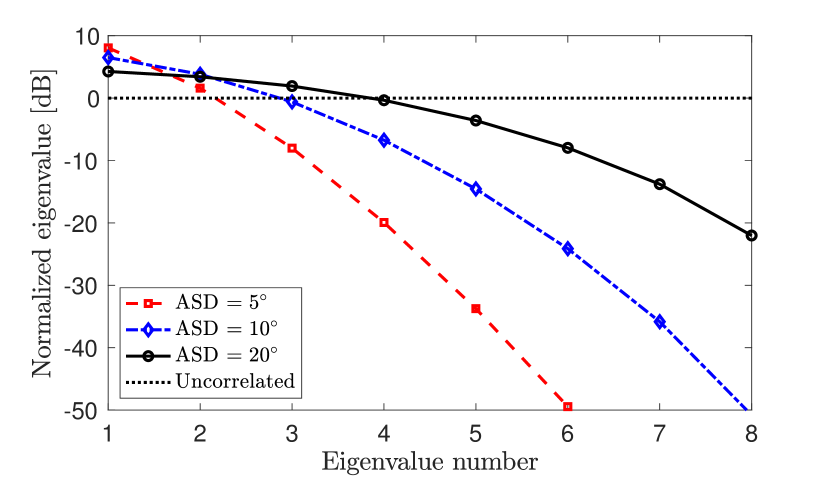
The main observation from Figure 2.6 is that the eigenvalues are widely different when the ASD is small, but the eigenvalue spread decreases with an increasing ASD. In the case of , the first four eigenvalues contribute to of the sum of the eigenvalues. Hence, the correlation matrix is nearly rank-deficient and all channel realizations will essentially be linear combinations of the corresponding four eigenvectors. In fact, the single largest (dominant) eigenvalue contributes to 80% of the sum. Therefore, most channel realizations will point in similar directions as the dominant eigenvector. The eigenvalue variations are substantially smaller for , but there is still a 425 times difference between the largest and smallest eigenvalues. This can be compared to the extreme case of uncorrelated fading, represented by the dotted curve, where all eigenvalues are identical.
Spatial correlation is of fundamental importance in Cellular Massive MIMO [Sanguinetti2019a], where the number of antennas is so large that the eigenvalue variations play a key role in mitigating interference between UEs [BjornsonHS17], [Huh2012a], [Yin2016a], [Yin2013a]. We refer to [massivemimobook, Sec. 2] for more details on the basic impact that spatial correlation can have on a multi-user system. Since the number of antennas per AP is envisaged to be fairly small in Cell-free Massive MIMO, spatial correlation cannot be utilized as efficiently but we will anyway consider it throughout this monograph. In particular, we will analyze the effect of the eigenvalue spread on the channel estimation performance in Section 4 on p. 4.
2.6 Channel Hardening and Favorable Propagation
In Cellular Massive MIMO systems, two important properties appear when employing a large number of antennas at an AP: channel hardening and favorable propagation. These properties provide an insightful explanation for the performance gain of Cellular Massive MIMO and are elaborated for channels featuring correlated fading in [massivemimobook, Sec. 2.5] and for some other types of channels in [Marzetta2016a, Ch. 7]. Whether these properties appear or not depends strongly on the number of antennas and the spatial channel correlation properties.
In this section, we define and analyze channel hardening and favorable propagation in Cell-free Massive MIMO, which are rather different from the cellular case since multiple APs serve each UE. There are several different definitions in the cellular literature and we have selected those that extend most naturally to the cell-free case. We will observe that the two properties are now affected not only by the spatial correlation and the total number of antennas in the network, , but also by the variations in the large-scale fading coefficients among the APs and the power allocation. Recall from Section 2.5.2 that the large-scale fading is determined by the distances between the APs and UEs, as well as other macroscopic propagation effects (e.g., shadow fading). We stress that, although we dedicate a section to describe when channel hardening and favorable propagation might appear in practice, these properties are not formally required to make use of any of the results presented in this monograph. We refer to [Chen2018b] for a more detailed analysis of the two properties in Cell-free Massive MIMO.
2.6.1 Channel Hardening
Each element of a channel vector takes a new independent realization in every coherence block, but these small-scale fading variations will not necessarily affect the communication performance. As can be seen in (2.10), the received downlink signal at UE contains the desired signal component , where the effective channel is
| (2.20) |
This is the summation of the inner product between the channel vector and the precoding vector from all the APs. The value of this effective channel can potentially remain almost constant even if the individual elements of the channel vectors are changing. More precisely, when the random realizations of the effective channel in (2.20) are close to the mean value (i.e., the variance is small), then approximately the same effective scalar channel will appear in every coherence block and we can, thus, operate the system as if we were communicating over a deterministic channel. When this happens, we say that we have achieved channel hardening, where the word “harden” refers to the fact that the effective channel is becoming more deterministic.
Definition and Sufficient Condition for Channel Hardening
To give a formal definition of the channel hardening property, we assume all serving APs apply MR precoding, which we define as
| (2.21) |
with determining how much power AP is assigning for transmission to UE . Note that MR is the precoding method that maximizes the received signal power at the UE. If we insert this precoding into (2.20), the effective channel becomes
| (2.22) |
Note that the following channel hardening definition considers the combined channel from all the serving APs to a particular UE , which is the natural extension of the definition in Cellular Massive MIMO where only a single AP serves each UE [massivemimobook, Sec. 2.5.1].
Definition 2.6.1 (Channel hardening).
For a given set of serving APs and downlink power allocation coefficients , the effective channel to UE is said to provide asymptotic channel hardening if
| (2.23) |
in the mean-squared sense as .444Convergence in the mean-squared sense also implies convergence in probability and in distribution. The exact type of convergence is of limited importance since we are not interested in the asymptotic regime but to get a structured way to evaluate when we can obtain approximate channel hardening for a finite number of antennas.
The expectation in (2.23) is computed with respect to the independent channel realizations in different coherence blocks, while and the power allocation coefficients are assumed to be constant.
This definition says that the effective channel in (2.22) is close to its mean value when the number of AP antennas grows large. Since the -length channel vectors become larger as more antennas are added, the underlying assumption is that the antenna arrays are deployed according to some distribution that determines the evolution of the channel statistics (e.g., spatial correlation matrices). This is why the convergence is specified in the mean-squared sense. When considering correlated Rayleigh fading, a sufficient condition for channel hardening is as follows.
Lemma 2.6.2.
For correlated Rayleigh fading channels, a sufficient condition for the effective channel of UE to provide asymptotic channel hardening is that
| (2.24) |
Proof 2.6.3.
The ratio in the left-hand side of (2.23) has a mean value of one, thus we want to prove convergence to the mean value. In this case, convergence in the mean-squared sense requires that the variance of the ratio goes asymptotically to zero. The variance can be computed as
| (2.25) |
by utilizing the statistical independence of the channels to the different APs and by applying [massivemimobook, Lemma B.14] to compute the expectations. We then obtain the sufficient condition in (2.24) by utilizing the definition of in (2.14), which implies that .
Although the definition of channel hardening relies on asymptotic arguments, we can use it to evaluate the degree of channel hardening for setups with a finite number of antennas. If the expression in (2.24) is close to zero, this means that the left-hand side of (2.23) is close to one and thus channel hardening is approximately achieved.
It has been shown in the Cellular Massive MIMO literature that spatial correlation reduces the convergence rate to channel hardening [massivemimobook, Sec. 2.5.1]; that is, more antennas are needed to achieve a certain degree of channel hardening. This can be also observed in (2.24) where can be computed as the sum of the squared eigenvalues of the spatial correlation matrix . Recall from Figure 2.6 that spatial correlation is represented by large eigenvalue variations. Since the sum of the eigenvalues equals by definition, the squared sum of the eigenvalues can take values between (when all eigenvalues equal to ) and (when there is only one non-zero eigenvalue that equals ). The latter represents an extreme case of high spatial correlation. To achieve a high degree of channel hardening, we want the expression in (2.24) to be small and the case when all eigenvalues are the same (i.e., no spatial correlation) achieves the smallest value.
Impact of the Number and Geographical Distribution of APs
In the context of Cell-free Massive MIMO, where each AP is supposed to have a relatively small number of antennas but there will be many APs instead, it is interesting to evaluate if one can compensate for having a small by having many APs. To analyze this further, we assume that so that there is no spatial correlation. The expression in (2.24) then simplifies to
| (2.26) |
If , or one AP has a much larger value on than the other APs that serve UE , then (2.26) becomes approximately . If we instead consider the case when all the serving APs have the same value of , then (2.26) becomes . Hence, it is plausible to achieve the same degree of channel hardening by having many APs with few antennas as with one AP with many antennas in some cases. If is the same for all the serving APs, it is only the total number of AP antennas that determines the degree of channel hardening. However, when the APs have different values of , then the total number of antennas needed to achieve a certain degree of channel hardening will likely be larger than in Cellular Massive MIMO.
The geographical distribution of the APs, with respect to the UE, determines the values of the large-scale fading coefficients . There can naturally be tens of dB differences between the serving APs, even if they have rather similar distances to the UE. One can compensate for this by applying a power allocation algorithm where the powers are selected to even out the differences. More precisely, we can reduce the power from nearby APs (with larger ) and increase the power from APs that are further away (with smaller ) to achieve roughly the same value of for all the serving APs. This will increase the degree of channel hardening but will not necessarily be desirable from an end-to-end performance perspective since we can achieve a higher total received power at the UE by allocating the same power in the opposite way (more power from the nearby APs).
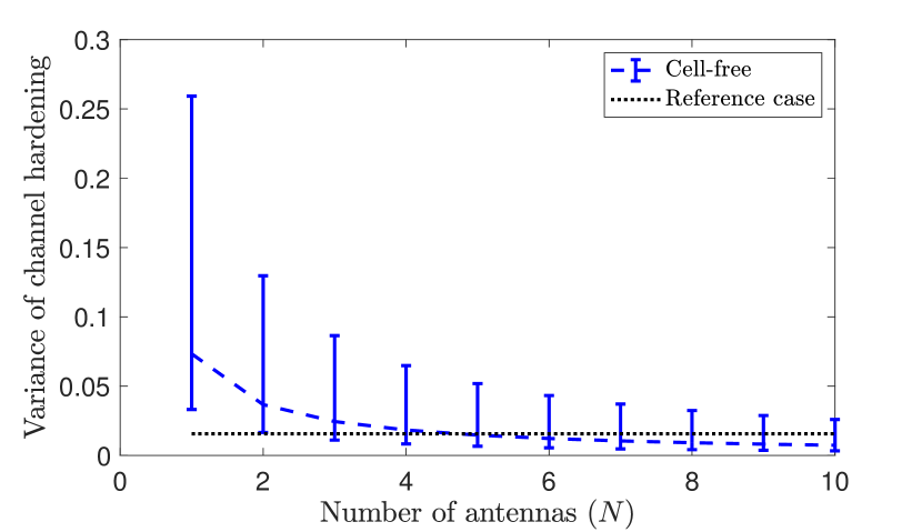
Figure 2.7 exemplifies how the degree of channel hardening depends on the geographical AP distribution and the number of antennas per AP. We consider the channel to a UE in the center of m m area. APs are uniformly distributed in the area and transmit with equal power to the UE. We use the large-scale fading model in (2.16) and assume independent and identically distributed (i.i.d.) Rayleigh fading. The figure shows the value of the expression in (2.26) for different values of . Since the value depends on the AP distribution, the dashed line shows the median value while the vertical bars indicate the interval in which 90% of all realizations occur. As a reference, the dotted horizontal line shows the value of (2.26) for a single AP with 64 antennas, which represents a Cellular Massive MIMO setup that would achieve a high degree of channel hardening. If single-antenna APs are used, then the degree of channel hardening is far from that of the reference case, even if the total number of antennas is the same. The median reaches the reference case for but half of the realizations give substantially larger values. It is first when the number of antennas per AP reaches 8 or 10 that the degree of channel hardening is comparable to that of Cellular Massive MIMO. Note that the total number of antennas is then an order of magnitude larger than in the reference case.
Takeaways
In summary, channel hardening is a desirable property but not mandatory for the operation of Cell-free Massive MIMO. In fact, we can expect a substantially lower degree of channel hardening in cell-free networks than in cellular networks when the number of serving antennas is the same. Channel hardening makes some capacity lower bounds (that we will present later in this monograph) closer to the true capacity and also serves as a motivation for not trying to optimize the power allocation in every coherence block but rather on average. We will return to these things later in this monograph.
Note that we defined channel hardening from a downlink precoding perspective in this section. The same argumentation can be made also in the uplink, in which case the precoding vectors are replaced by combining vectors, and the power allocation coefficients are replaced by weights that the CPU uses when fusing the signals from different APs. The details on this will be provided in Section 5 on p. 5.
2.6.2 Favorable Propagation
When multiple UEs are spatially multiplexed in the system, there will generally be interference between their transmissions, and the precoding/combining can be selected to strike a balance between achieving strong desired signals and causing little interference. However, if the UEs’ channels are spatially orthogonal, then the inter-user interference is automatically mitigated by MR processing so one can basically ignore it. When this happens, we say that favorable propagation is experienced.
If we consider the received downlink signal of UE in (2.10), then the interference caused by the concurrent transmission to UE is . If the MR precoding defined in (2.21) is utilized, then the effective interfering channel is
| (2.27) |
It is the magnitude of this term compared to the magnitude of the effective channel of the desired signal in (2.22) that determines how strong the interference is in relative terms. If the ratio is close to zero, then the interference will be negligible and we benefit from favorable propagation.
Definition and Sufficient Condition for Favorable Propagation
There are several different formal definitions of favorable propagation in the Cellular Massive MIMO literature but none of them is a perfect fit for the case when multiple APs are transmitting coherently. Hence, we provide the following new definition that is tailored to the cell-free scenario.
Definition 2.6.4 (Favorable propagation).
A given UE experiences asymptotically favorable propagation with respect to UE (with ) if
| (2.28) |
in the mean-squared sense as .
This definition says that the effective interfering channel in (2.27) (i.e., a weighted sum of the inner products between the channel vectors of the two UEs) should go asymptotically to zero, when it is normalized by the average value of the desired effective channel in (2.22). The weights are the downlink transmit powers. Note that the numerator depends on the set of APs that serve the interfering UE , while the denominator depends on the set of APs serving the considered UE . For correlated Rayleigh fading channels, a sufficient condition for favorable propagation is obtained as follows.
Lemma 2.6.5.
For correlated Rayleigh fading channels, a sufficient condition for UE to experience asymptotically favorable propagation with respect to UE is that
| (2.29) |
Proof 2.6.6.
The ratio in the left hand side of (2.28) has a mean value of zero, thus we want to prove convergence to the mean value. In this case, convergence in mean-squared sense requires that the variance of the ratio goes asymptotically to zero. The variance can be computed as
| (2.30) |
by utilizing the statistical independence of the channels to the different APs and by applying [massivemimobook, Lemma B.14] to compute the expectations. We then obtain the sufficient condition in (2.29) by utilizing the definition of in (2.14), which implies that .
Although the definition of favorable propagation relies on asymptotic arguments, we can use it to evaluate the degree of favorable propagation for setups with a finite number of antennas. If the expression in (2.29) is close to zero, this means that the left-hand side of (2.28) is close to zero and thus favorable propagation is approximately achieved.
The value of the expression in (2.29) depends on the spatial correlation properties in a nontrivial manner. The term in the numerator takes its largest value when the spatial correlation matrices and are identical up to a scaling factor, which represents the case when the two UEs have almost the same spatial directivity of their channels (statistically speaking). In contrast, the term takes its smallest value when the spatial correlation matrices have identical eigenvectors but the eigenvalues are matched together in the opposite order (i.e., large eigenvalues from one matrix are multiplied with small eigenvalues from the other matrix). This represents the case when the two UEs have very different spatial directivity. Clearly, it is the latter case that leads to the highest degree of favorable propagation.
Impact of the Geographical Distribution of APs
To instead focus on the different large-scale fading variations that the UEs experience, we can assume that so that there is no spatial correlation. The expression in (2.29) then simplifies to
| (2.31) |
This expression decays as so more antennas lead to a higher degree of favorable propagation. Moreover, the set of APs that serve UE plays an important role in determining the value of (2.31). If those APs are far from UE , all the terms in the numerator will likely be very small and then we can achieve favorable propagation even with . However, if , the numerator and denominator might be of comparable size and then we might need many antennas per AP to achieve favorable propagation. The power allocation also plays a key role; to make the term in the numerator small, we can either have a small value of and/or use a low transmit power on that AP.

Figure 2.8 exemplifies how the degree of favorable propagation depends on the geographical AP distribution, the distance between the UEs, and the number of antennas per AP. We consider the same setup as in Figure 2.7 but add an interfering UE that is either 10 m or 100 m to the east of the desired UE. We assume each UE is served by the 8 APs that provide the eight largest large-scale fading coefficients and these APs transmit with equal power. The figure shows the value of the expression in (2.31) for different . Since the value depends on the AP distribution, the dashed line shows the median value while the vertical bars indicate the interval in which 90% of all realizations occur. As a reference, the dotted horizontal line shows the value of (2.31) when a single AP with 64 antennas serves both UEs, which represents a Cellular Massive MIMO setup. We notice that the distance between the UEs strongly determines the degree of favorable propagation. When the UEs are close together, we need around antennas per AP before favorable propagation is approximately achieved. When the UEs are 100 m apart, most realizations of the AP locations lead to favorable propagation even for , but there are still large variations. We can expect that, in practice, some UEs that are far apart might still not achieve favorable propagation with respect to each other.
Takeaways
In summary, favorable propagation is a desirable property that makes inter-user interference disappear when using MR precoding (which does not actively suppress any interference). However, favorable propagation is not a necessary property. We have observed that UEs that are served by partially the same APs might not experience it with respect to each other. In those cases, the interference can instead be suppressed by using precoding methods that are actively suppressing interference. This is covered in detail in Section 6 on p. 6.
Note that we defined favorable propagation from a downlink precoding perspective in this section. The same argumentation can be made also in the uplink, as previously discussed in relation to channel hardening. When there is a lack of favorable propagation in the uplink, we can use receive combining to deal with the interference instead; see Section 5 on p. 5. Although there are clear mathematical similarities between channel hardening and favorable propagation, the properties are different. In particular, a UE might exhibit channel hardening but not favorable propagation or vice versa. It is also likely that some pairs of UEs will experience favorable propagation with respect to each other, while other pairs will not.
2.7 Summary of the Key Points in Section 2
Chapter 3 Theoretical Foundations
This section describes some basic results from estimation, information, and optimization theory which will be utilized later in this monograph. Section 3.1 describes the foundations of estimating Gaussian distributed random variables, which might be the channels in a cell-free network. Section 3.2 defines the channel capacity and describes standard methods for computing achievable lower bounds, which are also known as achievable spectral efficiencies (SEs). In Section 3.3, we consider the maximization of a ratio known as a generalized Rayleigh quotient. In Section 3.4, two different utility maximization algorithms are provided, which are of particular interest for the optimization of UE performance in a cell-free network. The key points are summarized in Section 3.5.
3.1 Estimation Theory for Gaussian Variables
The estimation of channel coefficients is an important aspect of any coherent communication system. In this section, we provide the theoretical foundation for estimating the realization of a Gaussian random variable from an observation that is corrupted by independent additive Gaussian noise. We only present the main concepts and results that will be used in later chapters and refer to textbooks such as [massivemimobook], [Kay1993a] for further details and explanations.
Definition 3.1.1 (Minimum mean-squared error estimator).
Consider arandom variable with support in and let denote an arbitrary estimator of based on the observation . The particular choice of that minimizes the mean-squared error (MSE)
| (3.1) |
is called the MMSE estimator of . It can be computed as
| (3.2) |
where is the conditional PDF of given the observation .
The MMSE estimator of a complex Gaussian random variable from an observation that is corrupted by independent additive complex Gaussian noise (and interference) can be computed in closed form.
Lemma 3.1.2.
Consider estimation of the -dimensional vector , with a positive semi-definite correlation matrix , from the observation . The pilot signal is known and is an independent noise/interference vector with a positive definite correlation matrix.
Proof 3.1.3.
The detailed proof can be found in [massivemimobook, App. B.4].
For brevity, we will denote the MMSE estimate as , without explicitly specifying what observation it was based on. A consequence of Lemma 3.1.2 is that the MMSE estimate is distributed as
| (3.6) |
Moreover, the estimation error is distributed as
| (3.7) |
These random variables are independent, which is a useful property that will be utilized in the analysis in future sections.
3.2 Capacity Bounds and Spectral Efficiency
The SE is the performance metric that will be used throughout this monograph. This is a measure of the average amount of information that can be correctly transferred per complex-valued sample, when a very large block of data is transmitted. This is the natural metric in broadband applications, where the demand for data is large.
Definition 3.2.1 (Spectral efficiency).
The achievable SE of an encoding/decoding scheme is the average number of bits of information, per complex-valued sample, that it can transmit reliably over the channel under consideration.
When communicating over a bandwidth of Hz, the Nyquist-Shannon sampling theorem specifies that the communication signal is fully determined by complex-valued samples per second [Shannon1949b] (or real-valued samples per second). These are the samples that the data is encoded into in communications and the SE describes the amount of data that can be transferred per such complex sample. Since there are samples per second, the unit of the SE is either bit per complex sample or bit per second per Hertz, which is abbreviated as bit/s/Hz. We will use the latter unit in the remainder of this monograph. A related metric is the information rate [bit/s], which is defined as the product of the SE and the bandwidth .
The channel between a given transmitter and receiver supports many different SEs (depending on the chosen encoding/decoding scheme), but the largest achievable SE is of key importance when designing communication systems. The maximum SE is determined by the so-called channel capacity. We refer to the original paper [Shannon1948a] by Shannon and textbooks on information theory, such as [Cover1991a], for the general and formal definition. In wireless communications, we are particularly interested in channels where the received signal is a superposition of a scaled version of the desired signal and additive Gaussian noise. These channels are commonly referred to as discrete memoryless additive white Gaussian noise (AWGN) channels, since each discrete input signal leads to a discrete output signal that is independent of previous and future inputs. We will provide exact capacity expressions and capacity lower bounds for two distinctly different cases: deterministic and random channels. Although the channels are modeled as random in this monograph, both cases will be utilized.
3.2.1 Capacity Bounds for Deterministic Channels
We begin with the canonical case when the channel is deterministic and the communication is only disturbed by Gaussian distributed noise. A block diagram of this setup is provided in Figure 3.1.
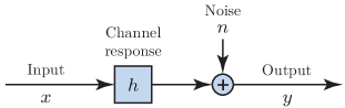
Lemma 3.2.2.
Consider a discrete memoryless AWGN channel with input and output given by
| (3.8) |
where is independent noise. The input distribution is power-limited as and the channel response is deterministic and known at the output.
In this case, any SE smaller or equal to the channel capacity
| (3.9) |
is achievable. The capacity is achieved by selecting .
Proof 3.2.3.
The detailed proof can be found in [Shannon1949b].
The practical meaning of the channel capacity is that for any SE smaller or equal to the capacity, there exists an encoding/decoding scheme such that an arbitrarily low error probability can be achieved. More precisely, if we consider an information sequence with scalar inputs to the AWGN channel, then the probability of error goes to zero as . This means that an infinite decoding delay is required to achieve the capacity. However, in practice, one can operate very close to the capacity whenever blocks of thousands of bits are transmitted [Bjornson2016b], which is typically the case in broadband applications.
The channel considered in Lemma 3.2.2 is called a single-input single-output (SISO) channel because one input signal is sent and results in one output signal. However, we will demonstrate in later sections how the same result can be utilized in situations with multiple antennas. The capacity expression in (3.9) has a form that is typical for communications: the base-two logarithm of one plus the SNR defined as
| (3.10) |
In the setups considered in this monograph, the communication is also disturbed by interference from other concurrent transmissions. In this case, the exact capacity is generally unknown, but convenient lower bounds can be obtained [Biglieri1998a]. The following lemma provides a lower bound on the capacity that will be used repeatedly in this monograph.
Lemma 3.2.4.
Consider a discrete memoryless interference channel with input and output given by
| (3.11) |
where is independent noise and is random interference with an arbitrary distribution that has zero mean, variance , and is uncorrelated with the input (i.e., ).
The input distribution is power-limited as and the channel response is deterministic and known at the output. The channel capacity is then lower bounded as
| (3.12) |
where the bound is achieved using the input distribution .
Proof 3.2.5.
The detailed proof can be found in [massivemimobook, App. C.1.2].
The lower bound on the capacity in (3.12) is achieved by encoding/decoding the signal as if the interference is independent Gaussian noise, because this is the worst case from a communication perspective [Hassibi2003a]. There are no approximations involved but the achievable SE is generally smaller than the capacity, particularly when there are very strong interfering signals. However, treating non-Gaussian interference as independent Gaussian noise in the encoding/decoding is practically convenient and provably optimal in the low-interference regime [Annapureddy2009a], [Annapureddy2011a], [Motahari2009a], [Shang2011b], [Shang2009b]. When we use the SE expression from Lemma 3.2.4 in later sections, the random interference term will not only include interference from other concurrent transmissions but also unknown random variations in the desired channel.
The SE expression in (3.12) has a similar form as the capacity expression in Lemma 3.2.2. It is the base-two logarithm of one plus the expression
| (3.13) |
which is an SINR. We will refer to it as an effective SINR, which means that the lower bound in (3.12) is effectively the same as the capacity of an AWGN channel with an SNR equal to in (3.13). This implies that the SE in (3.12) can be practically achieved using channel codes designed for AWGN channels.
3.2.2 Capacity Bounds for Random Channels
We consider randomly fading channels in this monograph. If the channel is a random variable that takes a new independent realization after a finite block of complex samples (e.g., a coherence block), then another capacity concept can be defined: the ergodic capacity. The transmission then spans asymptotically many realizations of the random variable that describes the channel and the word “ergodic” identifies that all the statistical properties of the channel are deducible from a single sequence of channel realizations. We begin with the canonical case when the communication is only disturbed by Gaussian distributed noise.
Lemma 3.2.6.
Consider a discrete memoryless channel with input and output given by
| (3.14) |
where is independent noise and the input distribution is power-limited as . The channel is a realization of a random variable that is independent of the signal and noise, and the realization is known at the receiver.
The ergodic channel capacity is
| (3.15) |
where the expectation is with respect to . The capacity is achieved by selecting the input distribution .
Proof 3.2.7.
The detailed proof can be found in [massivemimobook, App. C.1.1].
The ergodic capacity of the block-fading channel is similar to the capacity in (3.9), but the key difference is that there is an expectation in front of the logarithm in (3.15). In this case, is called the instantaneous SNR. We can also define the average SNR as
| (3.16) |
where the expectation is computed with respect to the channel realizations.
As mentioned above, the communication will be disturbed by interference from other concurrent transmissions in this monograph. In this case, the exact ergodic capacity is generally unknown, but a convenient lower bound can be obtained by once again treating the interference as noise [Biglieri1998a], [Medard2000a]. The following lemma provides a lower bound on the ergodic capacity that will be used repeatedly in this monograph.
Lemma 3.2.8.
Consider a discrete memoryless interference channel with input and output given by
| (3.17) |
where is independent noise, the channel response is known at the output, and is random interference with an arbitrary distribution satisfying the properties listed below. The input is power-limited as .
Suppose is a realization of the random variable and that is a random variable with realization that affects the interference variance. The realizations of these random variables are known at the output. If the noise is conditionally independent of given and , the interference has conditional zero mean (i.e., ) and conditional variance denoted by , and the interference is conditionally uncorrelated with the input (i.e., ), then the ergodic channel capacity is lower bounded as
| (3.18) |
where the expectation is taken with respect to and , and the bound is achieved using the input distribution .
Proof 3.2.9.
The detailed proof can be found in [massivemimobook, App. C.1.2].
Note that in Lemma 3.2.8, we used the shorthand notation for the conditional expectation . For notational convenience, we omit the random variables in similar expressions in the remainder of this monograph and only write out the realizations.
The lower bound on the ergodic capacity in (3.18) is an achievable SE and will often be called that in this monograph. Except for the list of technical conditions that must be satisfied, the SE in (3.18) is essentially the same as for the case of deterministic channels in (3.12), but with an expectation in front of the logarithm. The expression in (3.18) will be called the effective instantaneous SINR, because it takes the same role as the instantaneous SNR in the ergodic capacity expression in (3.15). In other words, the capacity lower bound is equivalent to the ergodic capacity of a fading AWGN channel where the instantaneous SNR is . This implies that the SE in (3.18) can be practically achieved using channel codes designed for fading AWGN channels.
When we use the SE expression result in Lemma 3.2.8 in later sections, the random interference term will not only include interference from other concurrent transmissions but also channel uncertainty due to estimation errors regarding the desired channel. In those cases, represents an estimate of the desired channel and represents the estimates of the interfering channels.
3.3 Maximization of Rayleigh Quotients
A commonly appearing problem formulation in multi-antenna communications is that of maximizing a power ratio between the desired signal and interference plus noise. The optimization variable is a vector determining how the signal observations made at the different receive antennas are weighted together. For example, consider the received signal at antennas. It is modeled as
| (3.19) |
where is a deterministic channel vector, is the random information signal with power , and is independent noise. If we apply a receive combining vector to (3.19), we get
| (3.20) |
and the SNR becomes
| (3.21) |
The type of expression in the right-hand side of (3.21) is known as a Rayleigh quotient111The expression in (3.21) is also known as the Rayleigh–Ritz ratio. Note that the only connection between Rayleigh fading and Rayleigh quotient is that they have been named after the same researcher. and can be maximized with respect to as follows.
Lemma 3.3.1.
For a given channel vector , it holds that
| (3.22) |
where the maximum is attained by .
Proof 3.3.2.
The Cauchy-Schwarz inequality for two vectors and says that
| (3.23) |
with equality if and only if and are linearly dependent. It follows that where the maximum is attained for (among other solutions where the vectors are linearly dependent).
The result in Lemma 3.3.1 is commonly used in signal processing and the optimal vector is known as MR combining or matched filtering. This method maximizes the SNR, however, it is a generalization that will be particularly useful in this monograph. Let us generalize (3.19) by replacing the i.i.d. noise term with the colored noise term having a positive definite covariance matrix . The new received signal is
| (3.24) |
and by applying a receive combining vector to (3.24), the SNR becomes
| (3.25) |
This type of expression is known as a generalized Rayleigh quotient and can be maximized with respect to as follows.
Lemma 3.3.3.
For a given channel vector and Hermitian positive definite matrix , it holds that
| (3.26) |
where the maximum is attained by or .
Proof 3.3.4.
The matrix square root of exists since is positive definite, thus we can define the new variable and establish that
| (3.27) |
The expression at the right-hand side is a Rayleigh quotient of the kind in Lemma 3.3.1 and, thus, maximized by . Hence, the solution to (3.26) is and the maximum value follows accordingly. Since any vector that is parallel to also achieves the maximum value, we can also use since
| (3.28) |
according to the matrix-inversion lemma (Lemma B.0.1 on p. B.0.1).
This lemma shows how to maximize a generalized Rayleigh quotient and what the maximum value is. The solution to (3.26) is not unique but for any will also maximize the expression. This lemma will be utilized several times in Section 5 on p. 5 to optimize different kinds of receiver processing in the uplink.
3.4 Optimization Algorithms for Utility Maximization
A utility function is a metric of system performance and can be formulated in different ways. In this section, we provide state-of-the-art optimization algorithms for solving two main types of utility maximization problems. These algorithms will be utilized in Section 7 on p. 7 to solve several resource allocation problems.
The SE is used in this monograph to measure the communication performance of each UE. When designing the network operation, there are different SEs to take into consideration and these are mutually conflicting due to interference. For example, we can improve the SE of one UE by reducing the transmit powers assigned to other UEs, but with the side-effect that the SEs achieved by the other UEs are then reduced. To identify a good tradeoff between the UEs’ individual performance, a scalar-valued utility function can be defined to take all the SEs into consideration. This is called scalarization in the field of multi-objective optimization [Bjornson2014c]. We will consider two utilities: max-min fairness and sum SE.
Since we have not provided any explicit SE expressions for User-centric Cell-free Massive MIMO systems yet, the presentation in this section is based on a generic SISO scenario. Suppose the received signal used for decoding the signal of UE can be expressed as
| (3.29) |
where denotes the normalized, independent random data signal of UE with and is the set of transmit power coefficients for all the UEs.222As we see in Section 6 on p. 6, there can be more than one transmit power coefficient per UE in the downlink. Although here we assume the length of the vector is , we can simply change it for the mentioned downlink power allocation optimization. The transmit powers are non-negative: , for . We write this as .
The received signal in (3.29) contains three parts. The term is the desired part, containing the data signal multiplied with a deterministic amplitude that is a function of (it usually only depends on ). The interference term contains the interfering data signal of UE , for , and the term is random and determines the strength of the interference caused to UE by UE . This term is also a function of . Note that we have included a self-interference term with a random amplitude , which we further assume to have zero mean. This term can model the uncertainty that the receiver has regarding the channel that the desired signal propagated over, which will be utilized and further explained in later sections. Finally, is the independent additive noise.
We obtain the following result by using Lemma 3.2.4.
Lemma 3.4.1.
Proof 3.4.2.
We obtain this result from Lemma 3.2.4 by letting be the received signal in the lemma, is the desired signal, is the channel response, and is the noise. The interference term is random with zero mean and variance since the data signals have zero mean, unit variance, and are independent. The condition is satisfied since was assumed to have zero mean.
With the notation provided by Lemma 3.4.1, the individual performance of the UEs are represented by their SEs , which are different performance metrics. For each choice of the transmit power vector , the UEs will achieve a certain combination of SEs that can be gathered in a -dimensional vector . By considering the set of all such vectors that can be obtained with feasible transmit power vectors (i.e., those satisfying a set of power constraints that exist in the system), we can generate a -dimensional region that represents all the possible ways of operating the system. This region is called an SE region and is exemplified in Figure 3.2 for . The shaded region contains all the feasible operating points. We need to select one of these points and there is no truly optimal way to do it. All the points in the interior of the region are strictly suboptimal since there are points at the outer boundary where all the UEs achieve higher SEs. On the other hand, each point on the outer boundary represents one possible tradeoff between the performance achieved by the different UEs. When comparing two points on the outer boundary, one UE will prefer the first point and another UE will prefer the second point. This conflict cannot be resolved in a fully objective manner but the network operator must inject a subjective opinion of what kind of operating point is preferred by the network as a whole.
As mentioned at the beginning of this section, we will adopt the scalarization approach to identify a tradeoff between the metrics [Bjornson2014c]. This means that we combine the SE metrics into a single scalar utility function representing the network-wide performance. We consider the two most common utility functions from the literature: max-min fairness and sum SE. These utilities represent two extremes in how to balance between transmitting many bits and obtaining user fairness. The max-min fairness utility requires every UE to get the same SE, which means that the optimal operating point in Figure 3.2 lies on a line from the origin with slope. As indicated in the figure, the max-min fairness solution is the point where this line intersects the outer boundary. The maximum sum SE is generally obtained at another operating point, as illustrated in Figure 3.2. It lies on a line with equation , where is the maximum achievable sum SE. While this point maximizes the number of bits that are transmitted in total, the downside is that the bits are unequally distributed among the UEs. In this example, UE 2 gets a smaller SE than at the max-min fairness point, while UE 1 gets a larger SE. In the remainder of this section, we will describe algorithms for finding these operating points in networks with arbitrarily many UEs.
3.4.1 Max-Min SE Fairness
The aim of max-min SE fairness is to maximize the lowest SE among all the UEs in the network, which is known as max-min fairness. Since the SE of UE in (3.30) is an increasing function of the effective SINR, , maximizing the minimum SE is the same as maximizing the minimum effective SINR among all the UEs. We assume there are linear constraints on the transmit power vector:
| (3.32) |
where the fixed vector specifies the weighting coefficient for each UE’s power coefficient and is the maximum allowed power,333This model can be utilized for both downlink and uplink power allocations. In the downlink, per-AP power constraints are considered, which leads to power constraints (one per AP). In this case, the non-zero elements of are multiplied with the power coefficients for the UEs that are served by AP . On the other hand, in the uplink, there are individual power constraints (one per UE). Hence, only the th element of the vector is non-zero while all other elements are zero. the max-min fairness problem can be formulated as
| (3.33) | ||||
To solve this problem, we first introduce the auxiliary variable that represents the lowest SINR among all the UEs. We can then obtain the following optimization problem that is equivalent to (3.33) in terms of having the same maximum utility value and optimal value of :
| (3.34) | ||||
The equivalence of the two problems can be verified by noting that is at most equal to the lowest SINR among the UEs and it should be equal to that value to maximize the objective function. The reformulation in (3.34) is known as the epigraph form of (3.33) [Boyd2004a, Sec. 3.1.7].
An optimal solution to the problem in (3.34) can be obtained by a bisection search over . To see this, let denote the optimal objective value of the problem in (3.34). If we select in (3.34), the problem will obviously be infeasible. On the other hand, if we select any , the problem in (3.34) is feasible. Hence, we can apply a bisection search over to find [Boyd2004a, Sec. 4.2.5]. At each iteration, we consider a value and need to solve the following feasibility problem:
| (3.35) | ||||
The goal of solving the feasibility problem in (3.35) is to find any solution that satisfies the constraints. The numerical precision that is needed to find the value of that corresponds to the global optimum can be extremely high, particularly if some variables in have a much smaller impact on the SINR of the UE with the worst channel conditions than the other variables. One can prove by contradiction that all UEs should get identical SINRs at the global optimum but this is only one of the many feasible solutions to the feasibility problem in (3.35) for any . We have noticed experimentally that this is a real issue when optimizing large cell-free networks, where some of the serving APs have much weaker channels than other serving APs. To improve the convergence rate, we will therefore replace the feasibility problem with a problem having the same constraints but where the total power is minimized as well. This will encourage numerical solvers to identify the feasible point where all UEs get the same SINR, while retaining optimality. By utilizing this property, we obtain Algorithm 1 where the revised subproblem is given in (3.36).
| (3.36) | ||||
Instead of solving a sequence of optimization problems, as in Algorithm 1, a fixed-point algorithm can be implemented when the SINR expression satisfies certain additional conditions stated in the next lemma from [Hong2014, Lemma 1, Theorem 1].
Lemma 3.4.3.
Suppose satisfy the following:
-
1.
if and if and only if , ;
-
2.
is strictly increasing with respect to and is strictly decreasing with respect to , for , when , ;
-
3.
For and , , .
The optimal solution to the optimization problem in (3.34) then satisfies and . Moreover, , for all and , for at least one .
Define and let denote the set of feasible that satisfies this last property:
| (3.37) |
The power vector computed by Algorithm 2 converges to the optimal solution to (3.34) if the following additional conditions are satisfied:
-
•
There exist numbers , , and a vector such that , for all ;
-
•
For any and : ;
-
•
For any and : and .
Whenever the conditions stated in Lemma 3.4.3 are satisfied, the fixed-point algorithm in Algorithm 2 should be utilized to solve the max-min fairness problem since it fully utilizes the SINR structure.
3.4.2 Sum SE Maximization
A potential drawback of the max-min SE fairness problem is that all the emphasis is put on the UEs with the worst channel conditions. When having a large network where every UE only causes interference to a small subset of neighboring UEs, it is likely that many UEs can achieve substantially larger SEs while barely affecting the UEs having the worst conditions. In these situations, it might be better to maximize the sum SE, which represents the total number of bits that are transmitted without considering how the bits are assigned between the UEs. The sum SE maximization problem can be expressed as
| (3.38) |
Note that the above problem is usually not convex and, hence, it is hard to obtain the optimal solution [Luo2008a]. There exist global optimization methods [Bjornson2013d], [Weeraddana2012a] that find the optimum but their computational complexity is unsuitable for real-time applications. A pragmatic solution is to instead settle for a local optimum. A common approach for finding a local optimum to sum SE maximization problems is the weighted MMSE method [Shi2011], which results in iterative algorithms.
To obtain the weighted MMSE reformulation of the sum SE maximization problem at hand, we recall the SISO channel for UE in (3.29) where the received signal is . The receiver can compute an estimate of the desired signal using a scalar combining coefficient that can amplify it and rotate the phase. The corresponding MSE is given by
| (3.39) |
and it is a convex function of . One can show that the value of that minimizes the MSE for UE in (3.39) for a given is
| (3.40) |
After plugging into (3.39), it follows that the corresponding is equal to .
The main idea of the weighted MMSE method is to introduce the auxiliary weight for the MSE and attempt to solve the following optimization problem:
| (3.41) | ||||
The problem is equivalent to the original sum SE maximization problem in (3.38) in the sense that they have the same global optimal solution. The equivalence of the two problems follows from the fact that the optimal in (3.41) is , which is equal to . Hence, we obtain the original sum SE maximization problem in (3.38) with the same constraints. The benefit of the reformulation in (3.41) is that we have the following result that is adapted from [Shi2011, Theorem 3].
Lemma 3.4.4.
| (3.42) | |||
When implementing Algorithm 3, the subproblem in (3.42) is required to be solved optimally with respect to (when the other variables are kept constant), otherwise, the block coordinate descent algorithm will not converge to a local optimum. Fortunately, the problem in (3.42) is convex for the power allocation problems we consider in Section 7 on p. 7 and the optimal solution can, thus, be obtained by any of the standard algorithms from convex optimization theory [Boyd2004a]. We elaborate further on this in Remark 7.1.3 on p. 7.1.3.
3.5 Summary of the Key Points in Section 3
Chapter 4 Channel Estimation
This section describes how channel estimation is carried out in User-centric Cell-free Massive MIMO systems based on the transmission of uplink pilots. The system model during pilot transmission is defined in Section 4.1. The MMSE channel estimation scheme is presented in Section 4.2. The impact of the cell-free architecture, interference from pilot-sharing UEs, and spatial correlation in the estimation process is evaluated in Section 4.3. A basic algorithm for pilot assignment and dynamic cooperation cluster formation is described in Section 4.4. The key points are summarized in Section 4.5.
4.1 Uplink Pilot Transmission
We consider the cell-free network defined in Section 2 on p. 2 where APs, each equipped with antennas, are arbitrarily distributed over the coverage area. The APs are connected to CPUs via fronthaul links. These can be used for sharing the CSI and channel statistics needed to decode the uplink data signals and precode the downlink data.
UE is served only by the APs with indices in the set , which is assumed fixed and known wherever needed. To perform coherent transmission processing (both between the antennas at each AP and across the cooperating APs), knowledge of the channel responses from the UEs to the serving APs is required. It is particularly important for AP to have estimates of the channel vector from UE if . Since the channels are assumed to be constant throughout one coherence block and change independently from one block to another, following the block fading model described in Section 2.3.1 on p. 2.3.1, they need to be estimated once per each coherence block. According to the TDD protocol defined in Section 2.3.2 on p. 2.3.2, samples are reserved for uplink pilot signaling in each coherence block. Therefore, each UE can transmit a pilot sequence that spans these samples and each AP can use the received signals to estimate the channel.
Ideally, we would like every UE to use a pilot sequence that is orthogonal to the pilots of all other UEs so there is no interference between the transmissions. However, since the pilots are -dimensional vectors, we can only find a set of at most mutually orthogonal sequences (i.e., a set of vectors that forms an orthogonal basis that spans ). The finite length of the coherence blocks imposes the constraint that makes it impossible to assign mutually orthogonal pilots to all UEs in practical networks with . Hence, we instead assume the network utilizes a set of mutually orthogonal pilot sequences that are designed to satisfy , for . One option is to use the columns of as pilot sequences. We refer to [massivemimobook, Sec. 3.1.1] for further examples of how to select pilot sequences. The only important aspect in the context of this monograph is that
| (4.1) |
These pilots are assigned to the UEs in a deterministic way, for example, when they get access to the network. We return to the pilot assignment problem in Section 4.4.
More than one UE might be assigned to each pilot sequence. We denote the index of the pilot assigned to UE as and define
| (4.2) |
as the set of UEs that use the same pilot as UE , including itself. The elements of are scaled by the square-root of the uplink transmit power of UE , which we denote as in the pilot transmission phase. The elements of are transmitted as the signal in (2.3) over consecutive samples. The received signal at AP during the entire pilot transmission is denoted as and is given by
| (4.3) |
where is the receiver noise with i.i.d. elements distributed as . The received uplink signal is the observation that AP can use to estimate the channels to all the UEs that it serves. The estimation can either be carried out directly at AP or be delegated to the CPU. In the latter case, AP acts as a relay and sends the received pilot signal to the CPU via the fronthaul link. The CPU can in principle compute all the channel estimates using the received pilot signals . However, since the channel vectors are independent, there is no loss of optimality if the channel estimates are computed separately at each AP in the set . The estimation results presented in this section apply to both cases.
4.2 MMSE Channel Estimation
Suppose we want to estimate (either at AP or at the CPU), based on the received pilot signal in (4.3). The first step is to remove the interference from UEs using orthogonal pilots by multiplying the received signal with the normalized conjugate of the associated pilot . This yields , given by
| (4.4) |
where the first term contains the desired channel scaled by , which is the square root of the total pilot power . The second term is the interference generated by the pilot-sharing UEs and the third term is the noise . The noise term has independent elements with variance since has i.i.d. -elements and is a vector with unit norm.
Note that is sufficient statistics for the estimation of since no information about or the pilot-sharing UEs’ channels is lost by multiplying with . This is a positive consequence of using mutually orthogonal pilots; if a larger set of partially overlapping pilots would be used instead, then many more UEs are partially sharing the same pilot dimensions and this would make the computation of the MMSE estimator more computationally involved. In our case, the resulting signal in (4.4) matches with the MMSE estimation structure in Lemma 3.1.2 on p. 3.1.2, leading to the following result.
Corollary 4.2.1.
Proof 4.2.2.
The MMSE estimator has this name because it minimizes the MSE among all possible estimators. The MMSE estimator in (4.5) is linear in the sense that is computed by multiplying the processed received signal with matrices. It is therefore sometimes called the linear MMSE estimator. However, we prefer to use the pure MMSE notion to make it clear that one cannot further reduce the MSE by using a non-linear estimator. Note that
| (4.10) |
so the correlation matrix of the channel estimate can also be expressed as . The distribution of in (4.7) allows us to generate random realizations of the channel estimate without having to compute the received signal as an intermediate step. It is convenient for both mathematical analysis and numerical simulations.
In practice, the computation of in (4.5) requires knowledge of two matrices:
-
1.
The spatial correlation matrix of ;
-
2.
The sum of the correlation matrices of pilot-sharing UEs and noise.
Both matrices depend on the statistics of the channels and thus are constant. Therefore, we can assume that the matrix can be precomputed. This matrix can be described by complex scalars, which can be exchanged via the fronthaul links to make available wherever needed (e.g., at AP or the CPU). The required fronthaul signaling is negligible since the channel statistics are deterministic and thus constant throughout the entire data transmission.111In practice, the channel statistics will change due to UE mobility or new scheduling decisions, but measurements suggest roughly two orders of magnitude slower variations compared to the channel vectors. If the matrix is precomputed, computing the MMSE estimate in a given coherence block entails first computing and then multiplying it with of each UE served by AP . The first operation requires complex multiplications per pilot sequence while the second needs complex multiplications per UE [massivemimobook, Sec. 3.4]. In summary, the computational complexity for channel estimation at AP is
| (4.11) |
per coherence block, if every UE that it serves uses a different pilot sequence (which is preferable). This value is scalable as if remains finite, which is in line with the sufficient condition for scalability presented in Lemma 2.4.2 on p. 2.4.2.
Remark 4.2.3 (Alternative estimation methods).
The MMSE estimator is the optimal choice when having full statistical knowledge, as assumed in this monograph (see Section 2.5.1 on p. 2.5.1). Note that each spatial correlation matrix contains elements and the computational complexity in (4.11) is proportional to . There are alternative channel estimators in the literature that provide larger MSEs, since the MMSE estimator is optimal, but can be useful to limit the computational complexity or deal with incomplete statistical knowledge. This can be of interest in Cellular Massive MIMO systems, where is large, since the complexity or overhead required to learn all the matrix elements can be substantial. However, none of these issues are pressing in Cell-free Massive MIMO, where is small, and will thus not be covered in this monograph. We refer to [massivemimobook, Sec. 3.4] for details on alternative estimators and to [BSD16A], [CaireC17a], [NeumannJU17], [Sanguinetti2019a], [UpadhyaJU17] for methods to estimate spatial correlation matrices in practice.
4.2.1 Normalized MSE
The value of the MSE depends on the average channel gain (among other factors) and a strong channel might have larger errors in absolute terms than a weaker channel. However, it is the relative size of the error that matters, not the absolute size. Hence, the estimation accuracy is quantified by considering the normalized MSE (NMSE). When it comes to the channel between AP and UE , the NMSE is defined as
| (4.12) |
and measures the relative estimation error variance per antenna. The NMSE is 0 when perfect estimation is achieved while it is 1 if so that we are only receiving noise and interference. In general, any reasonable estimator will provide an NMSE between 0 and 1, where smaller values are preferable.
In the case of single-antenna APs (i.e., ), the spatial correlation matrix reduces to the average channel gain and (4.12) simplifies to
| (4.13) |
which can be rewritten as
| (4.14) |
where
| (4.15) |
is the effective SNR of the pilot transmission from UE to AP . The word “effective” implies that the pilot processing gain is included in the SNR expression, which is achieved since the receiver processing in (4.4) coherently captures all the transmitted pilot energy without increasing the noise. If the pilot sequences are samples long, then the effective SNR is dB larger than the nominal SNR at a single sample. This gain is highly desirable for achieving good estimation quality also for UEs with limited transmit power and/or weak channel conditions.
Since it is the total pilot energy that determines , in practice, one can choose between spreading it over the samples of the pilot sequence or concentrating it into only one of them. The former solution keeps the peak-to-average-power ratio low but is sensitive to hardware imperfections; for example, a UE might only be able to approximately generate its pilot sequence, leading to only approximate orthogonality between the sequences that are meant to be orthogonal. This problem does not occur in the latter case since UEs with orthogonal pilots are transmitting at different samples of the coherence block. On the other hand, the concentration of pilot energy into specific samples corresponds to boosting their power, which is not possible in all implementations since it can increase the peak-to-average-power ratio. Generally speaking, the system can improve the effective SNR of the pilot transmission by either increasing the pilot length or boosting the pilot power on specific samples.
4.2.2 Pilot Contamination
From (4.13), it follows that the interference generated by the pilot-sharing UEs increases the NMSE, thereby reducing the channel estimation quality. In the case of multiple-antenna APs (i.e., ), the NMSE in (4.12) is exactly the same in (4.13) if uncorrelated Rayleigh fading is assumed (i.e., ). This means that there is neither an advantage nor a disadvantage in using multiple antennas at the APs in the absence of spatial correlation. With spatially correlated channels, the NMSE in (4.12) has a more complicated structure. It is clearly increased by the interference from the pilot-sharing UEs, which enters into in (4.6). Unlike (4.13), (4.12) depends not only on the average channel gains but on the full spatial correlation matrices , for . Intuitively, the NMSE should be better when the interfering UEs’ channels have very different spatial correlation properties than the desired UE. For example, if we know a priori that the channels of two UEs contain multipath components distributed over widely different sets of angular directions, then their corresponding spatial correlation matrices should have different dominant eigenspaces and this should somehow be beneficial during channel estimation. This intuition will be confirmed later on in Section 4.3.3.
The “pilot interference” generated by the pilot-sharing UEs is known as pilot contamination in the Cellular Massive MIMO literature and behaves differently from the receiver noise; it does not only reduce the estimation quality, but also makes the channel estimates of pilot-sharing UEs correlated. To see this, let us compare the MMSE estimate in (4.5) of UE with the estimate
| (4.16) |
of another UE using the same pilot. In this case, we have that and such that (4.16) can be rewritten as
| (4.17) |
By comparing (4.17) with (4.5), we notice that only the scalar and the first matrix differ. If is invertible, we can write the relation as
| (4.18) |
This implies that the two estimates are correlated, with the cross-correlation matrix given by
| (4.19) |
This happens although the true channels were assumed statistically independent (i.e., , for ). Observe that if there is no spatial correlation so that and , then the channel estimate in (4.17) for any will be the same as the channel estimate except for a scaling factor. In this case, the channel estimates are fully correlated.
In conclusion, UEs that transmit the same pilot sequence contaminate each others’ channel estimates, in the same way as in Cellular Massive MIMO systems [Marzetta2010a], [Sanguinetti2019a] and other types of cellular systems [Niemela2004a], [Sapienza2001a]. The contamination not only reduces the estimation quality (i.e., increases the NMSE) but also makes the channel estimates statistically dependent [Sanguinetti2019a]. This has an important impact beyond channel estimation, since the contamination makes it harder to mitigate interference between UEs that use the same pilot in uplink and downlink. This will be investigated in Sections 5 and 6 on p. 5 and p. 6, respectively.
4.2.3 MMSE Estimation of the Collective Channel
So far, we have considered the estimation of a channel vector between a generic AP and UE . To perform coherent processing of the signals at multiple APs, it is necessary to have knowledge of the collective channel defined in (2.15), where is the block-diagonal collective spatial correlation matrix. However, the estimate of from all APs to UE can be only partially computed since only the APs in are computing estimates of the channels and/or send their pilot signals to the CPU. This means that only the following partial channel estimate is known in a scalable cell-free network:
| (4.20) |
where is a block-diagonal matrix with being defined in (2.1) as for APs that serve UE and zero otherwise. Moreover, contains the inverses of the received pilot signal correlation matrices defined in (4.6). The estimation error is with . Note that so we use the former expression for brevity.
The NMSE of can be computed as
| (4.21) |
where follows from the block-diagonal structure of both and . The NMSE of the collective channel in (4.21) has a similar form as the NMSE of an individual AP-to-UE channel in (4.12). Note that (4.21) is not the sum or average of the individual NMSEs, but contains a summation of MSEs in the numerator normalized by a summation of channel gains.
In the case of single-antenna APs or uncorrelated Rayleigh fading, (4.21) can be simplified as
| (4.22) |
In any case, the presence of pilot-sharing UEs will increase the NMSE and create a correlation between their respective channel estimates.
4.3 Impact of Architecture, Contamination, & Spatial Correlation
We will exemplify how the estimation accuracy of the MMSE estimator is affected by the cell-free architecture, pilot contamination, and spatial correlation. The numerical examples will uncover some of the basic properties that determine the NMSE and its impact on communication performance.
4.3.1 Impact of the Cell-Free Architecture
To gain insights into the basic impact of channel estimation errors in cell-free networks, we begin by considering single-antenna APs and the estimation of the collective channel of an arbitrary UE that has a unique pilot sequence: . In this case, the NMSE in (4.22) reduces to
| (4.23) |
If one AP has a much larger value of its effective SNR than the other APs in , then (4.23) can be approximated as
| (4.24) |
with . This approximation is exact if or when all the serving APs have the same value of . However, when the APs have different values of , then the exact NMSE in (4.23) will be larger than the approximation in (4.24).
This fact is exemplified in Figure 4.1 where (4.23) is plotted for the case in which UE is served by APs, or just one of them. We assume that is fixed to dB while we let vary from dB to dB. There is one NMSE curve for the case when both APs serve the UE and two curves for the case when only one of the APs serves the UE. We observe that the NMSE with both APs is higher than the NMSE with only AP serving the UE if . In contrast, a lower NMSE is obtained for . This shows that having more than one serving AP is not necessarily improving the estimation accuracy of the collective channel.
To gain further insights into this, we revisit the simulation scenario from Figure 1.10 on p. 1.10, where a cell-free network was compared with a corresponding small-cell setup and a single-cell Massive MIMO setup. In the cell-free case, we consider single-antenna APs that are deployed on a square grid in a coverage area of m m as shown in Figure 1.9(c) on p. 1.9. The bandwidth is 10 MHz and the noise power is dBm. The channels are Rayleigh fading, the channel gains are modelled as in (1.1), and the propagation distances are computed assuming that the APs are deployed 10 m above the UE. Comparisons are made with a single-cell setup with a 64-antenna Massive MIMO AP (with uncorrelated Rayleigh fading) and with a cellular network consisting of small cells deployed at the same AP locations.
Figure 4.2 shows the average of the NMSE in (4.23) for different uniformly distributed UE positions. The pilot transmit power varies from mW to W and the pilot length is . When comparing the three setups, we notice that it is preferable to have many single-antenna APs rather than a single AP with a large co-located array (as in conventional Cellular Massive MIMO). However, the small-cell network achieves better average estimation accuracy than the cell-free architecture since the AP with the lowest NMSE is always chosen in the small-cell network. This is in agreement with the results of Figure 4.1 where the lowest NMSE is achieved when only using the AP with the best channel. However, this does not mean that the cell-free architecture will achieve a lower communication performance, but only that the varying estimation quality must be taken into account when the cell-free network is combining the received signals from multiple APs.
The SE gain of using a cell-free architecture will be quantified in later sections of this monograph, but we will give an indication of the performance gain by considering the SNR that is achieved in the data detection. Suppose only UE is active in the network, then the local estimate in (2.5) of the data signal can be expressed as
This is the data estimate at AP . All the local estimates of the serving APs are sent to a CPU where the final estimate of is obtained as
| (4.25) |
For simplicity, we assume the APs apply MR combining with and compute the resulting SNR as
| (4.26) |
where the expectations with respect to the channel estimates are computed using Lemma B.0.7 on p. B.0.7. We stress that this is only one of the many ways to compute SNRs in the presence of estimation errors.
Figure 4.3 shows the distribution of the SNR value in (4.26) achieved at different random UE locations. We consider the same setups as in Figure 4.2 and let mW. The results show that the cell-free network achieves a higher SNR in the data detection than the corresponding small-cell setup (and Cellular Massive MIMO). This happens despite the lower average estimation quality of the channel estimates, as reported in Figure 4.2. The reason is that the cell-free network achieves a beamforming gain by coherently processing the signals at multiple APs. An even larger benefit will be achieved in a setup with multiple UEs, where the cell-free system excels at mitigating interference, as first illustrated in Section 1.3.2 on p. 1.3.2. This will be thoroughly analyzed in later sections.
4.3.2 Impact of Pilot Contamination
We now shift focus to the impact of pilot contamination. We concentrate on an arbitrary single-antenna AP and assume that it wants to estimate the channel of UE , while UE uses the same pilot. From (4.14), we obtain
| (4.27) |
The NMSE increment caused by pilot contamination depends on how much the interference is affecting the term in the denominator of (4.27), which accounts for interference and noise. The contamination is small when the value is close to one. Figure 4.4 shows the NMSE of the desired channel estimate for dB and varying values of from to dB. The dotted lines correspond to the case without pilot contamination (i.e., ) and are reported as references. The NMSE increases when the interfering signal becomes stronger, particularly when the desired UE has a strong channel to the AP. However, the pilot contamination effect is negligible whenever the interfering signal is dB weaker than the noise. We can thus conclude that each UE is only sensitive to pilot contamination from UEs that are relatively close to its serving APs. Another implication is that the UEs that an AP serves should preferably have different pilot sequences to limit pilot contamination [Bjornson2020a], [Sabbagh2018a]. This is aligned with the Cellular Massive MIMO literature where orthogonal pilots are normally utilized within every cell but reused in different cells [massivemimobook], [Marzetta2016a].
The distance between the AP and the interfering UE is one of the main factors determining the SNR of the interfering signal. Figure 4.5 shows the effective SNR (4.15) as a function of the propagation distance using the same parameter values as in Figure 4.3. The SNR reduces with the distance but can be above the dB reference curve for several hundred meters. Hence, pilot contamination is a non-negligible issue in practice. However, it is a gradual effect so the largest impact occurs when the interfering UE is rather close to the AP. The effective SNR increases by 10 dB when increasing the pilot length from to , which affects both the desired signal and contaminating signal. Even if the signal-to-contamination ratio remains the same, the propagation distances for which pilot contamination is a problem will grow since it is determined by comparing the contamination with the noise. On the other hand, each pilot can be reused less frequently among the UEs when is increased. Hence, we can expect the use of longer pilots to be beneficial when it comes to limiting the pilot contamination, as long as we assign the pilots properly to the UEs. We return to this in Section 4.4. Importantly, the curves in Figure 4.5 will move up or down depending on the transmit power, bandwidth, and propagation model so it is not the exact numbers that matter but the general behavior.
4.3.3 Impact of Spatial Correlation
We now quantify the impact of spatial correlation among AP antennas on the channel estimation accuracy and pilot contamination.
Impact of Spatial Correlation on Estimation Accuracy
Consider the spatially correlated channel between an arbitrary AP and an arbitrary UE, where the UE and AP indices are dropped for simplicity. We assume the UE uses a unique pilot sequence, thus the NMSE in (4.12) can be simplified as
| (4.28) |
Let denote the eigenvalue decomposition of the spatial correlation matrix, where the columns of the unitary matrix contain the eigenvectors (also called eigendirections) and the diagonal matrix contains the corresponding non-negative eigenvalues where . By using the eigenvalue decomposition, the NMSE in (4.28) can be rewritten as
| (4.29) |
where the second equality follows from moving the matrices and into the inverse, applying the cyclic shift property of the trace (see the second identity in Lemma B.0.2 on p. B.0.2), and utilizing that . An important observation from (4.3.3) is that the NMSE depends on the eigenvalues but not on the eigenvectors. This is a direct consequence of the fact that the estimation error correlation matrix has the same eigenvectors as the spatial correlation matrix [massivemimobook, Sec. 3.3].
We cannot change the spatial correlation matrices of a practical channel, but it is anyway important to understand what impact the correlation has. To this end, we now search for the eigenvalue distributions that maximize and minimize the NMSE under the constraint that . We will make use of the following result.
Lemma 4.3.1.
The function of the eigenvalue vector given in (4.3.3) is strictly concave on its domain.
A consequence of the strict concavity stated in Lemma 4.3.1 is that the maximum value of the NMSE in (4.3.3) under the average channel gain constraint is unique and achieved when all eigenvalues are equal: , for . This shows that, among all the spatial correlation matrices that satisfy , the uncorrelated fading model with provides the largest NMSE.
To identify the spatial correlation that instead minimizes the NMSE, we need the following lemma.
Lemma 4.3.3.
Suppose the eigenvalues of are sorted in decaying order:
| (4.30) |
where is the rank. Let denote the corresponding eigenvalue vector. Then, where .
This lemma provides a procedure for reducing the NMSE by modifying the two smallest non-zero eigenvalues of the correlation matrix. More precisely, they are replaced with one eigenvalue being the sum of two smallest non-zero eigenvalues and one eigenvalue being identically zero. If we repeat this procedure multiple times, we will progressively reduce the NMSE and eventually reach the case when , and , for , which provides the smallest possible NMSE among all spatial correlation matrices that satisfy . This corresponds to the case where is a rank-one matrix and thus represents the strongest type of spatial correlation. Any rank-one correlation matrix with the same achieves the same estimation accuracy. The conclusion is that the higher the spatial correlation is, the easier it is to estimate the channel since there is more structure to be utilized by the estimator.
The above properties are illustrated numerically in Figure 4.6, where the NMSE is shown for the local scattering model in (2.18), as a function of the azimuth ASD . The results are averaged over different nominal azimuth angles, while the elevation angle is fixed at and the elevation ASD is either or . The effective SNR (4.15) is 10 dB and there are antennas at the AP. Figure 4.6 shows that the NMSE is smaller when the ASD reduces (i.e., with higher spatial correlation). The NMSE for uncorrelated channels is shown in Figure 4.6 as a reference. For strongly spatially correlated channels, the NMSE can be one order of magnitude smaller than in the uncorrelated case, but this benefit is basically lost when . The ASD in the elevation dimension only affects the NMSE when the ASD in the azimuth dimension is small. The lower bound for fully correlated channels is attained in the extreme case of .
The impact of the number of AP antennas is studied in Figure 4.7 using the same correlation model as in Figure 4.6 but with the ASDs . The NMSE is shown as a function of the number of antennas for effective SNRs of , , and dB. The NMSE reduces as the number of AP antennas increases since the channel realizations observed at adjacent antennas are strongly correlated, which is utilized by the MMSE estimator to improve the estimation quality. However, only marginal gains are observed for , irrespective of the effective SNR. This happens when the ULA has become so wide that the outmost antennas experience almost uncorrelated channel realizations.
Impact of Spatial Correlation on Pilot Contamination
Next, we will analyze the impact of spatial correlation on pilot contamination. Assume UE and UE use the same pilot sequence and consider an arbitrary AP whose index is omitted. The NMSE of UE 1 in (4.12) takes the form
| (4.31) |
Unlike the NMSE in (4.27) for single-antenna APs, (4.31) depends not only on the effective SNRs but also on the full spatial correlation matrices and of the UEs. We now observe that (4.31) can be lower bounded by Lemma B.0.5 on p. B.0.5 as
| (4.32) |
where the equality occurs if and only if the correlation matrices are spatially orthogonal . This condition means that the eigenspaces are non-overlapping. If or , the condition can only be satisfied if both and are rank-deficient.
In the case of spatially orthogonal correlation matrices (i.e., ), the NMSE is completely unaffected by the interfering UE. Therefore, in theory, it is possible to completely avoid pilot contamination between the UEs. While the orthogonality condition is unlikely to hold in practice, a good rule-of-thumb is to assign pilots to the UEs such that is small.
Figure 4.8 shows the NMSE of the estimate of the desired channel with antennas. The spatial correlation is modeled by the local scattering model with elevation angles and ASDs , . The azimuth angle of the desired UE is , while the azimuth angle of the interfering UE is varied between and . The effective SNR of the desired UE is 10 dB and the interfering signal either has the same SNR or is 20 dB weaker. When the UE angles are well-separated, the NMSE is below , irrespective of how strong the interfering pilot signal is. This shows that pilot contamination has a minor impact on the estimation quality when the UEs have well-separated eigenspaces. The NMSE increases when the UEs have similar angles and reaches a peak at . The variations are large when the interfering UE has a strong channel to the AP, while the variations are small when the interfering signal is 20 dB weaker. The figure also includes reference curves for the case of uncorrelated fading, where the NMSE is angle-independent. We notice that the NMSE with correlated fading is always lower (or equal) to the NMSE with uncorrelated fading, even in the worst-case scenario where the desired and interfering UEs have identical angles. Hence, spatial channel correlation is helpful in practice to improve the estimation quality under pilot contamination.
4.4 Pilot Assignment and Dynamic Cooperation Cluster Formation
The mutually orthogonal pilots must be reused among the UEs and can be assigned to them in an effort to limit the pilot contamination effect. The examples given earlier in this section have demonstrated that this entails keeping a large physical distance between the pilot-sharing UEs, so that each AP that serves a given UE will be subject to pilot contamination that drowns in the receiver noise. This is a good way of picturing what we want to achieve when performing a pilot assignment but it is a simplification since the observations were made using a propagation model in which the SNR is a strictly decreasing function of the distance. In reality, the SNR and propagation distance are correlated, but there is also a fair amount of random variations that can be modeled as shadow fading. Hence, when designing pilot assignment algorithms, we should not take geometric parameters, such as the locations on a map, as input but instead consider the spatial correlation matrices . Those matrices are describing both the average channel gains , including shadow fading, and the spatial channel characteristics.
The pilot assignment is a combinatorial problem. There are possible assignments in a setup with UEs and pilots, thus the complexity of evaluating all of them grows exponentially with the number of UEs. The implication is that only suboptimal methods are feasible in practice. We will present one such algorithm in this section, and it will be utilized for performance evaluation in later sections. The algorithm will iteratively assign pilots to the UEs by always selecting the one that leads to the least pilot contamination. This is a so-called greedy algorithm and comes with no performance guarantees, but it will effectively avoid worst-case situations where closely spaced UEs (i.e., UEs with similar SNRs) are assigned to the same pilot. It is also practically attractive since the pilot assignment decision for a UE is made locally at a neighboring AP, instead of involving all APs in the network. We will provide a literature review of alternative pilot assignment methods in Section 7.4 on p. 7.4.
The formation of the DCC is tightly connected to the pilot assignment. We noted earlier in this section that a single-antenna AP can only reasonably serve one UE per pilot, namely the one having the strongest channel gain. The reason is that this UE would cause strong pilot contamination to all the pilot-sharing UEs if the AP tried to serve some of those UEs as well. Consequently, a basic algorithm for cluster formation is to first assign pilots to the UEs and then let each AP serve exactly UEs; for every pilot, the AP serves the UE with the strongest channel gain among the subset of UEs that have been assigned that pilot. This is most likely a suboptimal algorithm, particularly for multiple-antenna APs which could use spatial correlation to distinguish between UEs that send the same pilot and thereby serve multiple UEs per pilot if they have nearly non-overlapping eigenspaces (recall Figure 4.8). However, it makes good practical sense since every AP can make its clustering decisions locally. This is the clustering algorithm that will be utilized for performance evaluation in later sections. We will provide a literature review of alternative methods in Section 7.5 on p. 7.5.
An Algorithm for Joint Pilot Assignment and Cluster Formation
The basic pilot assignment algorithm consists of two steps. First, the UEs with indices from to are assigned mutually orthogonal pilots: UE uses pilot for . The remaining UEs, with indices from to , are then assigned pilots one after the other. UE begins by determining which AP it has the strongest channel to. The index of this AP is computed as
| (4.33) |
Since AP is expected to contribute strongly to the service of UE , it is preferable to assign UE to the pilot for which AP experiences the least pilot contamination. Hence, for each pilot , the AP can compute the sum of the average channel gains of the UEs that have already been assigned to that pilot. The AP then identifies the index of the pilot where the pilot interference is minimized:
| (4.34) |
This pilot is assigned to the UE and the algorithm then continues with the next UE. When all the UEs have been assigned to pilots, the clusters can be created. Each AP goes through each pilot and identifies which of the UEs have the largest channel gain among those using that pilot. The AP will serve that UE. The procedure is summarized in Algorithm 1.
This algorithm resembles the ones proposed in [Bjornson2020a], [Chen2016a]. The key idea was that whenever a new UE is admitted to the network, it begins by identifying the AP that it has the strongest channel gain to. In practical systems, the APs are periodically broadcasting synchronization signals to convey basic access information. The channel gains can be measured based on these signals. The accessing UE computes according to (4.33) and appoints AP as its Master AP. Note that this selection is made in a user-centric manner. The UE also uses the broadcasted signal to synchronize to the AP. The UE can contact its Master AP via a standard random access procedure [sanguinetti13bis], [Sesia09]. The Master AP computes the preferred pilot using (4.34) and informs the surrounding APs of the existence of the new UE. The surrounding APs can then determine if they should change which UEs to serve on pilot . This is a dynamic variation of Algorithm 1 that can be applied when new UEs are entering the system. It can also be applied when a UE has moved to such a large extent that its channel statistics have changed and, therefore, it can be treated as a new UE [Bjornson2020a], [Chen2016a]. The three main steps of this initial access algorithm are illustrated in Figure 4.9.
The algorithm described above is distributed in the sense that each UE is managed separately and each AP makes its pilot assignment decisions and cluster formation locally. A key challenge for any distributed cluster formation algorithm, including Algorithm 1, is the risk that some UEs will not be served by any AP. This can happen when a particular AP has the strongest channel to more than UEs, while it is only allowed to serve at most of them. A solution to this problem is to require that each UE is served by at least one AP, namely AP that is selected according to (4.33) [Bjornson2020a]. This will lead to pilot contamination but at least guarantees that each UE is being served. Since the intended operating regime of Cell-free Massive MIMO is the ultra-dense regime of , each AP will on average only have the strongest channel to UEs. Hence, if , there is a very low risk that one AP will have the strongest channel to more than ten UEs, but it can happen.
Remark 4.4.1 (Pilot decontamination).
Specific signal processing algorithms have been developed for situations where pilot contamination is the main performance-limiting factor. The general aim is to expand the dimension of the pilot sequences and we will briefly describe three main categories of such pilot decontamination approaches. The first category utilizes channel statistics, particularly spatial channel correlation, to assign pilots to UEs to proactively limit the pilot contamination effect. Some key references from the Cellular Massive MIMO literature are [BjornsonHS17], [Huh2012a], [Yin2013a], [Xu2015a], but these are not directly applicable to cell-free networks where each AP has a small number of antennas. Approaches developed for cell-free networks will be described in Section 7.4 on p. 7.4. The second approach is to make use of the uplink data as additional pilots, which is known as semi-blind or data-aided estimation [Carvalho1997a]. The main complication is that the data is unknown, but since long sequences of random data samples are fairly orthogonal, the transmitted signals will fall into different subspaces that can be identified by the receiving AP. Some key references from the Cellular Massive MIMO literature are [Ma2014a], [Mueller2014b], [Neumann2014a], [Ngo2012a], [Vinogradova2016a], [Yin2016a]. The existing algorithms rely on asymptotic properties that occur when and are jointly growing large, thus they are not applicable in cell-free networks where is small. The third approach is to superimpose low-power pilot sequences onto the uplink data, thereby making the pilot length equal to the number of uplink samples per coherence block. The benefit is that many more orthogonal pilot sequences can be generated, while the drawback is that the pilots and data will now mutually interfere. There are situations where it brings benefits, as exemplified in [Upadhya2014a], [Upadhya2017b], [Verenzuela2017a], [Verenzuela2020a] for Cellular Massive MIMO. However, it cannot increase the capacity scaling at high SNR, which is achievable by reserving certain dimensions for pilots [Zheng2002a]. We will not cover any of these methods in detail in this monograph, because it will later become apparent that pilot contamination is not a main limiting factor in Cell-free Massive MIMO.
4.5 Summary of the Key Points in Section 4
Chapter 5 Uplink Operation
This section describes two different uplink implementations of User-centric Cell-free Massive MIMO, which are characterized by different degrees of cooperation among the APs. Section 5.1 considers a centralized operation in which the pilot and data signals received at all APs are gathered (through the fronthaul links) at the CPU, which performs channel estimation and data detection. The achievable SE is derived based on the MMSE channel estimates and used to obtain the optimal, but unscalable, centralized receive combining. Alternative scalable combining schemes are then proposed. In Section 5.2, the SE analysis and design of scalable receive combining schemes are extended to a distributed operation where the local MMSE channel estimates are used at the APs to obtain local estimates of the UE data, which are then gathered and linearly combined at the CPU for final detection. To exemplify the performance and properties of cell-free networks under somewhat realistic conditions, a simulation setup is defined in Section 5.3 that will be used as a running example in the remainder of this monograph. Performance analysis and comparisons are carried out in Section 5.4, while a summary of the key points is provided in Section 5.5.
5.1 Centralized Uplink Operation
The most advanced uplink implementation of Cell-free Massive MIMO is a fully centralized operation, where the APs only act as remote-radio heads or relays that forward their received baseband signals to the CPU for processing. More precisely, each AP sends the received pilot signals in (4.4) and the received uplink data signal in (2.3) to the CPU, which performs channel estimation, receive combining and data detection. The centralized operation is illustrated in Figure 5.1(a). Although we call it centralized operation, this should not be interpreted as building a network that gathers the information related to all UEs at a single point at the center of the network. As described in Section 1.1 on p. 1.1, the CPU is a logical entity and its tasks can be divided between many geographically distributed edge-cloud processors [Interdonato2019a], as illustrated in Figure 1.3 on p. 1.3. Different UEs might use different processors. Hence, in practice, centralized operation means that each UE is associated with one nearby processor which we refer to as “the CPU” and all its serving APs send their respective received uplink signals to it. We will now explain what processing is done at the CPU and quantify the achievable uplink SE.
For each UE , the pilot signals are individually used at the CPU to compute the partial MMSE estimates of the collective channels from all UEs to the APs that serve UE (i.e., the APs with indices ). The estimation procedure was described in Section 4.2 on p. 4.2. Recall that is a block-diagonal matrix with being defined in (2.1) as for APs that serve UE and zero otherwise.
The received uplink data signals at the serving APs are jointly used at the CPU to compute an estimate of the signal transmitted by UE . From the signal model in Section 2.3.3 on p. 2.3.3, this is achieved by summing up the inner products between the effective receive combining vectors and for . This yields the estimate
| (5.1) |
where is the centralized combining vector and is the collective uplink data signal given by
| (5.2) |
with being the collective noise vector. Notice that (5.2) depends on all the channel vectors since all the APs receive the signal from all UEs. Since implies in (5.1), the CPU will however apply receive combining using only the data signals of the APs with . In other words, (5.1) can be equivalently written as by including only the subset of APs that serves UE in the summation. While this alternative expression is more compact at this point, it would require much more notation if used for performance analysis. That is why we utilize (5.1) in this section.
The expression in (5.2) is mathematically equivalent to the signal model of an uplink single-cell Massive MIMO system with correlated fading [massivemimobook, Sec. 2.3.1], if one treats the CPU as a receiver equipped with antennas. However, there are some key differences:
-
1.
Multiple UEs that are managed by the CPU are using the same pilot, which is normally avoided in single-cell systems.
-
2.
The antennas are distributed over different geographical locations. Hence, the collective channel is distributed as where the spatial correlation matrix has a block-diagonal structure, which is normally not the case in single-cell systems.
-
3.
Not all antennas are being used for signal detection, but only those belonging to the APs that serve the particular UE.
Despite these distinct differences, we can compute an achievable uplink SE, based on the knowledge of the partial MMSE estimates , using the methodology from the Cellular Massive MIMO literature [massivemimobook, Sec. 4.1]. From this expression, we can further obtain the optimal centralized receive combining vector . All the analysis in this section relies on the assumption that the spatial correlation matrices are perfectly known at the CPU to perform channel estimation, receive combining and data detection. We will return to this assumption in Section 5.1.5.
5.1.1 Spectral Efficiency With Centralized Operation
While the ergodic capacity of fully cooperative networks with perfect CSI is known in some cases [Estella2019a], it is generally unknown in the considered case with imperfect CSI. However, we can rigorously analyze the performance by using the standard capacity lower bounds described in Section 3.2 on p. 3.2. As a first step, we use (5.2) to rewrite (5.1) as
| (5.3) |
where the desired signal term has been divided into two parts: one that is received over the known partially estimated channel from UE and one that is received over the unknown part of the channel, represented by the estimation error . The former part can be utilized straight away for signal detection, while the latter part is less useful since only the distribution of the estimation error is known, as reported in Section 4.2.3 on p. 4.2.3. An achievable SE can be computed by treating the latter part as additional interference in the signal detection, by utilizing Lemma 3.2.8 on p. 3.2.8. If the first term in (5.1.1) is treated as the desired part while the other three terms are treated as noise in the receiver, the following SE is achievable.
Theorem 5.1.1.
An achievable SE of UE in the centralized operation is
| (5.4) |
where the instantaneous effective SINR is given by
| (5.5) |
with
| (5.6) |
and the expectation is with respect to the channel estimates. The matrix is the error correlation matrix of the collective channel .
The pre-log factor in (5.4) is the fraction of each coherence block that is used for uplink data transmission. The term takes the form of an “effective instantaneous SINR” [massivemimobook], with the desired signal power received over the estimated channel in the numerator and the interference plus noise in the denominator. More precisely, the numerator contains , while the first term in the denominator is the interference that is received over the estimated parts of the interfering channels, is the combined spatial correlation matrix of the signals received over the unknown parts of the channels, and the last term in the denominator is the noise power after receive combining. Notice that the matrix is the error correlation matrix of the collective channel ; see Section 4.2.3 on p. 4.2.3. We call (5.5) an “effective” instantaneous SINR since it cannot be measured in the system at any particular point in time, because the averaging over the estimation errors does not occur instantaneously. However, the SE is effectively the same as that of a fading single-antenna single-user channel where (5.5) is the instantaneously measurable SNR and the receiver has perfect CSI. In particular, this means that the desired data signal can be encoded and the received signal can be decoded as if we would communicate over such a fading AWGN channel.
The SE expression in Theorem 5.1.1 is not in closed form since there is an expectation in front of the logarithm in (5.4). However, the SE can be easily computed numerically using Monte Carlo methods, which means that we approximate the expectation with an average over a large number of random realizations. More precisely, we can generate realizations of the channel estimates in a large set of coherence blocks and compute the value of the logarithm for each one of them, followed by taking the sample mean of these values.
Theorem 5.1.1 is rather general in the sense that the SE is derived using the DCC framework and considering multi-antenna APs with arbitrary correlated fading channels and arbitrary DCC. The case of was considered in [Attarifar2020a], [Nayebi2016a], [Riera2018a], [Yang2019a], while [Bashar2018a], [Chen2018b] considered with uncorrelated fading and [Bjornson2019c], [Bjornson2020a] considered with correlated fading. In the extreme case when all APs are serving UE (i.e., ), the SINR in (5.5) can be simplified to
| (5.7) |
5.1.2 An Alternative Spectral Efficiency Expression
The SE expression in Theorem 5.1.1 is a lower bound on the capacity that is derived by utilizing the property that the channel estimate and the estimation error are independent random vectors. This condition is satisfied when using the MMSE estimator and Rayleigh fading channels as assumed in this monograph. An alternative bound that can be applied along with any channel estimator and fading model is the so-called use-and-then-forget (UatF) that is widely used in Cellular Massive MIMO [massivemimobook, Theorem 4.4], and also in Cell-free Massive MIMO [Bashar2019a], [Bjornson2019c], [Nayebi2016a] with for all and specific combining vectors. The name comes from the fact that the channel estimates are used for computing the receive combining vectors and then effectively “forgotten” before the signal detection takes place. In the considered network setting with multiple-antenna APs, arbitrary correlated fading channels, and arbitrary DCC, the following achievable SE is found by applying the UatF bound.
Theorem 5.1.3.
An achievable SE of UE in the centralized operation is
| (5.8) |
where the effective SINR is given by
| (5.9) |
and the expectation is with respect to the channel realizations.
Intuitively, in (5.8) should be smaller than in (5.4) since it relies on a simplified implementation in which the channel estimates are not used at the CPU for signal detection. This conjecture is hard to prove analytically but has been verified by numerous numerical experiments. Except for Section 5.4 where will compare with , we will not use in the remainder of this section, to avoid underestimating the achievable performance. However, we stress that one benefit with the simplified bound in Theorem 5.1.3 is that there is no expectation in front of the logarithm, because the bounding technique is treating the channel as deterministic. We will return to the expression in Section 7.1.1 on p. 7.1.1 where the uplink powers will be optimized by making use of the fact that there are only expectations at the inside of the logarithm.
5.1.3 Optimal Receive Combining
The SE expression in (5.4) holds for any receive combining vector but we would like to use the one that maximizes its value. We first note that we can multiply with any non-zero scalar without affecting the SINR value, since all the terms in the ratio are scaled equivalently. Hence, the goal of designing the receive combining is not to find the right length of the vector but the right direction in the vector space. We notice that (5.5) has the form of a generalized Rayleigh quotient:
| (5.10) |
where we have replaced by in the last term of the denominator by using the relation . Hence, the SINR can be maximized as described in Lemma 3.3.3 on p. 3.3.3. This leads to the following optimal combining vector.
Corollary 5.1.5.
The instantaneous SINR in (5.5) for UE is maximized by the MMSE combining vector
| (5.11) |
which leads to the maximum value
| (5.12) |
Proof 5.1.6.
We can maximize (5.5) by using Lemma 3.3.3 on p. 3.3.3 with , , and . To handle that might not be positive definite (but only positive semi-definite), we can regularize it by replacing with . This makes invertible and will not affect the final result since the inverse is then multiplied with , which removes the extra noise that was added to the unused dimensions.
The optimal combining vector in (5.11) consists of two parts: 1) the partial estimate of the channel to UE and 2) the inverse of a matrix that equals (plus the regularization term that is added to the unused dimensions), which is the conditional correlation matrix of the received signal, given the channel estimates. The first part identifies the combining vector that would maximize the desired signal power, while the second part rotates that vector to strike a balance between achieving a strong signal and suppressing interference. Note that the matrix inverse acts as a spatial whitening filter, as exemplified in Figure 5.2. The left graph in this figure shows how the received power of the desired signal and interference are arriving from different azimuth angles, while the noise is equally distributed over all angles. The goal of the receive combining is to identify the dashed direction where the SINR is maximized, which is clearly different from the direction where the signal is the strongest. By applying a spatial whitening filter, we obtain the graph at the right where the sum of the signal, interference, and noise powers is constant in all directions. We can then easily maximize the SINR by selecting the “direction” in the transformed domain where the signal is stronger, which automatically implies that the sum of the interference plus noise is at its lowest value.
It can be shown that the combining vector that maximizes the instantaneous SINR also minimizes the MSE in the data detection, which is defined as
| (5.13) |
This is the conditional MSE between the true data signal and the estimate of it from (5.1.1); see [massivemimobook, Sec. 4.1] for a deeper discussion. This is the reason why is generally called MMSE combining. This type of receive combining maximizes the mutual information of many types of channels with multiple receive antennas [Park2013a]. However, the particular expression in (5.11) is unique for Cell-free Massive MIMO with the centralized operation and the DCC framework.
Note that in (5.11) is always non-zero except when , which is an uninteresting special case since the CPU only needs to apply receive combining when at least one AP serves the UE. This implies that the CPU needs to compute all the MMSE channel estimates corresponding to any AP that is serving UE (i.e., APs with index ). The total number of complex multiplications required for channel estimation is reported in Table 5.1 and is computed as discussed above (4.11). In addition, we need to account for the complexity of computing the combining vector in (5.11) for once per coherence block. This complexity can be computed using the framework described in [massivemimobook, App. B.1.1] and exploiting the fact that only a subset of the APs takes part in estimating the transmitted signal ; see Remark 5.1.7 below for further details. Table 5.1 summarizes the total number of complex multiplications required for the computation of the MMSE combining vector of a generic UE . Since this number grows linearly with , the optimal MMSE combining makes the network unscalable according to Definition 2.4.1 on p. 2.4.1. We will, therefore, look for alternatives.
Remark 5.1.7 (Computation of MMSE combining).
The complexity of computing the MMSE combining vector of UE in (5.11) depends on the number of serving APs , not the total number of APs. To observe this, recall that is a block-diagonal matrix with being if AP serves UE (i.e., ) and zero otherwise. Therefore, the elements of and whose indices correspond to the zeros of do not affect any term in (5.11). In particular, suppose the APs with index are the serving ones. The computations will then be as shown in Figure 5.3, where only the shaded parts are non-zero. Only the upper block of size needs to be inverted and then multiplied with a vector of length . The total number of complex multiplications required for these two operations can be obtained by using the framework described in [massivemimobook, App. B.1.1] and is summarized in Table 5.1. If the serving APs have arbitrary indices, the computational complexity remains the same since the implementation can simply reorder the APs so that the serving ones are listed first.
| Scheme | Channel estimation | Combining vector computation |
|---|---|---|
| MMSE | ||
| P-MMSE | ||
| P-RZF | ||
| MR |
5.1.4 Scalable Combining Schemes for Centralized Operation
We will now develop centralized receive combining schemes that are scalable, in the sense that the computational complexity per UE is independent of . The simplest solution is to use MR combining with
| (5.14) |
which maximizes the numerator of the effective SINR in (5.5). In other words, the power of the desired signal is maximized while the existence of interference and estimation errors is ignored. Since the MMSE channel estimate is directly used as the MR combining vector, the computational complexity is equal to that of obtaining the partial MMSE channel estimate . This requires a total of complex multiplications, which is summarized in Table 5.1. Since no additional computations are needed, MR combining is a scalable solution with low complexity. However, we will observe later that the performance can be poor in the presence of interference, since a high degree of favorable propagation cannot be guaranteed between all UEs (see Section 2.6.2 on p. 2.6.2). Two scalable combining schemes that are superior to MR, in terms of dealing with interference, are therefore derived next by taking inspiration from the optimal MMSE combining in (5.11).
Partial MMSE Combining
In a large cell-free network with distributed UEs, it is reasonable to believe that the interference that affects UE is mainly generated by a small subset of the other UEs, which are located in the neighborhood of UE . We want to utilize this observation to reduce the computational complexity of the optimal MMSE combining and thereby achieve a scalable alternative. To this end, we assume that only the UEs that are served by partially the same APs as UE should be included in the inverse matrix in (5.11). These UEs have indices in the set
| (5.15) |
By utilizing , an alternative partial MMSE (P-MMSE) scheme can be defined as follows [Attarifar2020a], [Bjornson2020a], [Nayebi2016a]:
| (5.16) |
with
| (5.17) |
This scheme is not designed to be optimal from an SE perspective but as a scalable approximation of the optimal MMSE combining. We note that P-MMSE combining coincides with MMSE combining only when UE is served by all APs; that is, and . Another way to view this is that P-MMSE combining would be optimal if only the UEs with indices in were active. However, MMSE combining and P-MMSE combining are generally different schemes.
In Section 4.4 on p. 4.4, a DCC selection method was described where each AP serves exactly one UE per pilot sequence, which guarantees for all . Using this scheme, if all the APs that serve UE co-serve the same set of UEs. This is the smallest value that can take. Moreover, it holds that , where the upper bound is achieved in the unlikely case that all the APs in serve UE but otherwise serve entirely non-overlapping sets of UEs. Importantly, even this unlikely upper bound is independent of . The number of complex multiplications required by P-MMSE for channel estimation and combining vector computation is reported in Table 5.1. In computing those numbers, we have taken into account the discussion from Remark 5.1.7 that only the number of serving APs affects the size of the matrix inverse and matrix-vector multiplication. The exact expression is rather lengthy but, importantly, it is independent of , which makes P-MMSE a scalable combining scheme that supports an arbitrarily large number of UEs.
In practice, some fine-tuning can be done to improve the performance of P-MMSE by including additional UEs in to deal with strongly interfering UEs that are only served by other APs. A proper selection of these extra UEs will increase network performance without violating the scalability. However, in this monograph, we stick to the definition of in (5.15) for brevity.
Partial Regularized Zero-Forcing Combining
The complexity of computing the P-MMSE combining vector scales with . Each AP is supposed to have a relatively small number of antennas in cell-free networks, but might be large when there are many APs in the vicinity of UE . Since the combining vector is computed at the CPU, which is assumed to have high computational capability, the complexity might not be an issue. However, it is nevertheless interesting to explore if a further complexity reduction can be achieved without affecting the performance to any great extent. We will therefore present an alternative receive combining scheme, which is obtained as a simplification of P-MMSE. To this end, we note that if the channel conditions of the interfering UEs in are good, all the corresponding estimation error correlation matrices in will be small. If we neglect in (5.16), we obtain
| (5.18) |
This change has a negligible impact on the complexity but it enables further reformulation. Let us construct by stacking all the vectors with indices with the first column being . We further define as a diagonal matrix containing the transmit powers for , listed in the same order as the columns of . By letting denote the operation of only keeping the first column of its matrix argument, we can reformulate (5.18) as
| (5.19) |
where the second equality follows from the first identity of Lemma B.0.2 on p. B.0.2 and the third equality utilizes the fact that .
We call (5.19) partial regularized zero-forcing (P-RZF) combining. This name indicates that the matrix expression in (5.19) has the same form as the pseudo-inverse to the partial channel matrix . The only difference is that the inverse has been regularized by adding the matrix containing the noise variance and transmit powers. Combining vectors based on pseudo-inverses force the interference between the UEs to zero, but might lead to large losses in the desired signal power when the UEs have similar channels. P-RZF is balancing between suppressing interference and maintaining strong desired signal powers.
The total number of complex multiplications required for channel estimation and combining vector computation with P-RZF is reported in Table 5.1. As expected, this number is independent of . Hence, this scheme is also scalable. The main benefit over the P-MMSE is that an matrix is inverted in (5.19) instead of an matrix as in (5.16), which can substantially reduce the complexity since we typically have in cell-free networks. Most likely, this benefit comes with an SE loss since, in general, the channel conditions will not be so good to every interfering UE so that the estimation errors can be ignored. The tradeoff will be evaluated later.
5.1.5 Fronthaul Signaling Load for Centralized Operation
We wrap up the analysis of the centralized operation by quantifying the required fronthaul signaling. We will do this by counting the number of complex scalars that must be sent over the fronthaul links. In practice, these scalars will have to be quantized and different types of information can be quantized using a different number of bits per scalar. However, if all the scalars are sent over the fronthaul using the same bit precision, counting the number of scalars is sufficient to compare the signal load of different methods.
In each coherence block, AP needs to send complex scalars representing the pilot signals and complex scalars representing the received data signal . As summarized in Table 5.2, this requires a total of complex scalars, irrespective of the combining scheme used for detection at the CPU.111Note that is an upper bound on the fronthaul signaling load for pilot signals, which is achieved in the case that AP assigns all the available pilots to the UEs that it is serving. This was assumed by the pilot assignment scheme presented in Section 4.4 on p. 4.4, but is not the case in general. In other cases, AP exchanges a lower number of complex scalars for the pilot signals through the fronthaul links. Since this value does not grow with , we can conclude that the fronthaul signaling is scalable.
Notice that the implementations of the MMSE channel estimator and the P-MMSE combining scheme require knowledge of the spatial correlation matrices . In a centralized network, where the APs only act as relays, this information can be acquired directly at the CPU by using one of the pilot signaling methods that already exist in Cellular Massive MIMO literature (see [Sanguinetti2019a] for an overview). Hence, there is no need to exchange the spatial correlation matrices through the fronthaul links. As discussed later in Section 5.2.3, the situation is different in the distributed implementation presented next, where the pilot signals are not sent to the CPU but used locally at the APs for channel estimation. Statistical information must then be acquired at the APs and gathered at the CPU using the fronthaul.
| Implementation | Per coherence block | Statistics |
|---|---|---|
| Centralized | ||
| Distributed: opt LSFD | ||
| Distributed: n-opt LSFD | ||
| Distributed: no LSFD |
5.2 Distributed Uplink Operation
Instead of entirely delegating the channel estimation and data detection to the CPU, a User-centric Cell-free Massive MIMO network can be implemented to carry out as much of the signal processing as possible in a distributed manner. A motivating factor is that each AP can easily be equipped with a baseband processor that is (at least) as powerful as those in the UEs, thus algorithms that can make efficient use of it should be developed. The goal is to enable an ultra-dense deployment with , where the CPU’s capabilities are dimensioned based on the number of UEs, but largely unaffected by the number of APs. In other words, we should be able to add new APs to the network without having to upgrade the CPUs, thanks to the property that each AP comes with a local processor. Another reason is to reduce the fronthaul signaling compared to the centralized operation and to avoid the fronthaul quantization distortion, which exists in practice but is neglected in this monograph. Since a key property of cell-free networks is that multiple APs are involved in the service of each UE, the final data detection must be carried out at a point where the inputs from multiple APs are combined. Recall that the CPU is a logical entity so the unavoidable CPU tasks can be physically assigned to a nearby edge-cloud processor (or even one of the serving APs), so there is no need for a physical central unit. The following two-stage procedure is called distributed operation in this monograph and is schematically described in Figure 5.1(b).
In the first stage, each AP uses its received pilot signals to locally estimate the channels . For each UE , the AP can then use the local estimates to select a local receive combining vector . According to (2.5), the AP then computes its local estimate of as
| (5.20) |
Note that this estimate is zero for , thus AP only needs to compute (5.20) for the UEs that is serves.
In the second stage, the local data estimates of all APs are gathered at the CPU where they are combined/fused into a final estimate of the UE data. The CPU computes its estimate as a linear combination of the local estimates:
| (5.21) |
where is the weight that the CPU assigns to the local signal estimate that AP has of the signal from UE . Note that we include all the AP indices since for and the results do not change. To limit the fronthaul signaling, the APs are only sending the local data estimates to the CPU and not the channel estimates. Hence, the CPU needs to select the weights as a deterministic function of the channel statistics. Intuitively, the CPU should assign a larger weight to an AP having a large SNR to the UE than an AP having a small SNR, but also the interference situation and receive combining scheme should be taken into consideration.
The structure of the second stage resembles what is called large-scale fading decoding (LSFD) and was originally used in Cellular Massive MIMO [Adhikary2017a], [ashikhmin2012pilot]. Unlike the centralized operation, the two-stage procedure outlined above allows the network to make use of the distributed processing capabilities of the APs. The received signals are primarily processed at the points where they were received. Even if it the operation is not entirely distributed, it is as distributed as a cell-free network, utilizing coherent cooperation between APs, can become since only the final signal detection is done at the CPU.
The achievable SE for arbitrary local receive combining and LSFD weights will be derived next. After that, we will show how to make a judicious selection of the local combining vectors and how to compute the optimal LSFD weights. Since the preferred solutions turn out to be unscalable for networks with many UEs, we will provide scalable alternatives.
5.2.1 Spectral Efficiency and Optimal LSFD Weights
We will now compute an SE expression for UE in the distributed operation. Plugging (2.3) into (5.21) yields
| (5.22) |
where represents the noise. For brevity, we define the vector computed as
| (5.23) |
This is the vector with the receive-combined channels between UE and all APs that serve UE . Using this notation, (5.22) can be expressed as
| (5.24) |
where is the LSFD weight vector of UE . The realizations of change in every coherence block, while is supposed to be a deterministic vector that the CPU can select without knowing the channel realizations. We notice that (5.24) has the structure of a single-antenna channel where represent the effective channels of the different UEs. Although the effective channel is unknown at the CPU, we notice that its average is deterministic and non-zero if the receive combining is properly selected. Therefore, it can be assumed known222When dealing with ergodic capacities, all deterministic parameters can be assumed known without loss of generality, because these can be estimated using a finite number of transmission resources, while the capacity is only achieved as the amount of transmission resources goes to infinity. Hence, the estimation overhead for obtaining deterministic parameters is negligible. and used to compute the following achievable SE.
Theorem 5.2.1.
An achievable SE of UE in the distributed operation is
| (5.25) |
where the effective SINR is given by
| (5.26) |
and
| (5.27) |
The pre-log factor in (5.25) is the fraction of each coherence block that is used for uplink data transmission. The term takes the form of an effective SINR and is the ratio of the signal power term and a term containing noise and interference (including some self-interference from the desired signal due to the imperfect channel knowledge). Recall that the word “effective” refers to that this SE is effectively the same as that of a deterministic single-antenna single-user channel where (5.26) is the SNR and the receiver has perfect CSI. In particular, this means that the desired data signal can be encoded and the received signal can be decoded as if we would communicate over such an AWGN channel.
The SE expression in (5.25) is very general. Although this monograph considers correlated Rayleigh fading channels and MMSE channel estimation, (5.25) is actually a valid SE for any channel estimator and channel model, in contrast to the SE expression in (5.4) which is explicitly using those assumptions. This was previously discussed in Section 5.1.2.
The achievable SE in (5.25) holds for any local receive combining and LSFD vector , but we are naturally seeking a combination that makes the SE as high as possible. We start with considering the local receive combining vectors. Since AP locally selects for , without receiving input from other APs, there is no way for its combining scheme to be optimal from a network-wide perspective. However, the AP can do as well as it can by optimizing a local performance metric. Recall from Section 5.1.3 that the optimal receive combining in a centralized implementation minimizes the MSE in the data detection. In analogy with this result, we can let AP select the receive combining giving the best local estimate in terms of minimal conditional MSE:
| (5.28) |
The combining vector that minimizes (5.28) is
| (5.29) |
where is the error correlation matrix given in (4.9). This can be proved by computing the conditional expectation in (5.28) and equating its first derivative with respect to to zero. One can also show that (5.29) is the combining vector that would maximize the SE if AP detected the data signal locally. We call (5.29) Local MMSE (L-MMSE) combining to distinguish it from the MMSE combining in (5.11), which is applied at the CPU in the centralized operation. L-MMSE and MMSE combining coincide (except for that the latter is padded with zeros) in the special case when only AP serves UE (i.e., ). Hence, the computational complexity of L-MMSE is the same as for MMSE combining in Table 5.1 but with . Since this complexity grows with , we notice that L-MMSE combining is not a scalable combining scheme.
We now shift focus to the LSFD weights . For any given local receive combining vectors, can be optimized by the CPU to maximize the SE. Since it is a deterministic vector, it is optimized as a function of the channel statistics. We notice that (5.26) is a generalized Rayleigh quotient with respect to . Hence, we can maximize the effective SINR by using Lemma 3.3.3 on p. 3.3.3. The optimal is thus obtained as follows.
Corollary 5.2.3.
The effective SINR in (5.26) for UE is maximized by
| (5.30) |
where is the diagonal matrix with the th element being one if and zero otherwise. This leads to the maximum value
| (5.31) |
Proof 5.2.4.
We can maximize (5.26) by using Lemma 3.3.3 on p. 3.3.3 with , , and . The term is not present in (5.26) but has been added to make positive definite and thereby invertible.333Alternatively, pseudo-inverses could have been used in (5.30) and (5.31), but the end result will be the same since . This addition will not affect the result since .
This corollary provides the optimal (opt) LSFD vector that maximizes the effective SINR in (5.26). The optimal vector has a structure resembling that of MMSE combining since it is also computed to maximize a generalized Rayleigh quotient. The evaluation of in (5.30) requires knowledge of the -dimensional statistical vector , the Hermitian complex matrix , for , and the diagonal elements of the real-valued matrix . These statistical vectors and matrices can be computed at the APs, based on the received uplink signals and their choices of local combining vectors. The CPU is unable to compute them locally since it does not have access to those signals, thus the APs need to send these statistical parameters to the CPU through the fronthaul links. We will quantify the fronthaul signaling load in Section 5.2.3 but it is clear that the number of parameters grows with , thus making the use of the opt LSFD vector unscalable according to Definition 2.4.1 on p. 2.4.1.
We notice that the elements of , for all , and whose indices correspond to the zero rows of are all zero. By following the approach outlined in Remark 5.1.7, the computation of can be carried out while ignoring the APs that are not serving UE (see also Figure 5.3). The corresponding elements of can be set to zero and the computation of only requires the inversion of a matrix and multiplication of it by an -length vector, which corresponds to complex multiplications. This is reported in Table 5.3.
Remark 5.2.5 (Tightness of the capacity bound).
The SE expressionpresented in Theorem 5.2.1 is derived based on the UatF bound from the Cellular Massive MIMO literature [massivemimobook], [Marzetta2016a] in which the channel estimates are used for receive combining but “forgotten” when detecting the data. While this bounding principle is artificial when applied in cellular networks, where the combining and signal detection are carried out at the same place, it makes good sense in cell-free networks where each AP carries out local combining based on its local CSI and the CPU carries out the data detection without CSI.
Signal detection without access to channel knowledge generally leads to rather poor performance since the receiver does not know the desired channel realization but only its mean value . However, if there is a high degree of channel hardening so that , the capacity bound in Theorem 5.2.1 is expected to be close to the SE that we would get if is perfectly known. As shown in Section 2.6.1 on p. 2.6.1, there is no guarantee that this will be the case in cell-free networks; the degree of channel hardening can be low when having a small number of antennas per AP [Chen2018b]. In that case, the SE expression in (5.25) underestimates the practically achievable SE, but it is anyway the state-of-the-art capacity lower bound and will be used in this monograph. We will evaluate the tightness of the bound later in this section.
5.2.2 Scalable Schemes for Distributed Operation
While the L-MMSE combining in (5.29) and the opt LSFD vector in (5.30) are the preferable schemes in the distributed operation, none of these schemes is scalable. The former one has a computational complexity that increases with the number of UEs in the whole network and the latter one requires a fronthaul signaling load that grows in the same way. Therefore, we will now present suboptimal but scalable alternatives that are inspired by the aforementioned methods.
Scalable Local Receive Combining
We begin by revisiting the problem of selecting the combining vectors for at AP . Recall that L-MMSE in (5.29) is not a scalable scheme since it makes use of estimates of the channels from all UEs. To achieve scalability, the selection can instead be made as a function of the estimates of the channels from the UEs that AP is serving.
The simplest solution is to utilize MR combining [Nayebi2016a], [Ngo2017b], which is given by
| (5.32) |
One key benefit of using this scheme is that the combining vector follows directly from the channel estimates so that no additional computations are needed. The total number of complex multiplications is and is reported in Table 5.3. Another benefit is that all the expectations in Theorem 5.2.1 can be computed analytically, so the SE is available in closed form.
Corollary 5.2.6.
If MR combining with is used, then the expectations in (5.26) become
| (5.33) |
with for and
| (5.34) |
while
| (5.35) |
The results from Corollary 5.2.6 can be inserted into the instantaneous effective SINR in (5.26) to obtain a closed-form SE expression. However, the final expression is lengthy so we will only present it in the case of , where it can be substantially simplified.
Corollary 5.2.8.
If each AP has antenna, then the MMSE estimate of the scalar channel has variance
| (5.36) |
The instantaneous effective SINR, , in (5.26) then becomes
| (5.37) |
Proof 5.2.9.
The closed-form effective SINR in (5.37) shows the key behaviors of the cell-free operation. The signal term in the numerator contains the transmit power multiplied with a term containing the weighted sum of the contributions from the serving APs. Each AP contributes with a term proportional to the variance of its channel estimate, since the combining vector is based on that estimate. The coherent combination of the contributions from the different APs is represented by the square of the sum. The first term in the denominator contains non-coherent interference, which means that it is a summation of the powers of the individual interfering signals at the serving APs without any squares. Each term is multiplied with a scaling factor containing the LSFD weight and the scaling made by the MR combining. The second term in the denominator is the additional coherent interference caused by pilot contamination, which has a similar shape as the signal term. The third term is the noise power.
If local MR combining is used along with the LSFD vector , then the result of the distributed operation is equivalent to MR combining in the centralized operation. In other words, centralized MR combining can be implemented in a distributed fashion. However, MR is expected to perform poorly in the presence of interference, unless a high degree of favorable propagation is achieved, which is not guaranteed in cell-free networks (see Section 2.6.2 on p. 2.6.2). Therefore, we will also consider combining schemes that can suppress interference while still being scalable.
| Scheme | Channel estimation | Combining vector computation |
|---|---|---|
| opt (and n-opt) LSFD | ||
| L-MMSE | ||
| LP-MMSE | ||
| MR |
Inspired by the scalable P-MMSE combining in (5.16) that was designed for centralized operation, we can define the local P-MMSE (LP-MMSE) at AP based on only the channel estimates and statistics of UEs that are served by this AP (i.e., ). By starting from (5.29) but taking a summation over only the UEs in , instead of all UEs, we obtain the local combining vector
| (5.39) |
The number of complex multiplications required by LP-MMSE is reported in Table 5.3. Since this number is independent of , LP-MMSE is a scalable solution as . Compared to P-MMSE in (5.16) that was proposed for centralized operation, LP-MMSE has a substantially lower complexity per UE since it requires to compute the inverse of an matrix, rather than an matrix. Note that LP-MMSE coincides with L-MMSE when AP serves all the UEs (i.e., ). Unlike MR, the expectations in (5.26) and (5.31) cannot be computed in closed form when using LP-MMSE, but can be computed numerically using Monte Carlo methods, as will be done later in this section.
Remark 5.2.10 (Local P-RZF).
Since the complexity of P-MMSE is rather high in the centralized operation, we presented an alternative simplified P-RZF scheme with lower complexity. A similar simplification is not needed in the distributed operation since LP-MMSE already has a rather low complexity.
Scalable Large-Scale Fading Decoding
The opt LSFD vector in Corollary 5.2.3 is also not scalable for implementation in large networks. The bottleneck originates from the fact that all UEs in the network affect the interference levels at all APs, thereby determining how accurate the local data estimates are. To identify a scalable way to select for UE , we need to limit how many interfering UEs are considered in the computation.
The simplest solution is to give all the serving APs equal importance by setting [Nayebi2017a], [Ngo2017b]. In this case, the CPU takes the local estimates of the data from UE and sum them up to create the final data estimate
| (5.40) |
We call this approach no LSFD since the LSFD weights are basically omitted. The reason is that the original works on Cell-free Massive MIMO considered this solution, while LSFD weights were introduced only later. The key benefit is that no statistical parameters are needed at the CPU to compute (5.40).444To be more precise, no statistical parameters are needed to compute or (5.40), but the data detection leading to the SE in Theorem 5.2.1 requires that the signal strength and interference variance are known at the CPU. The main drawback is that equal importance is given to all APs when computing (5.40), even if some APs might be subject to high interference or low SNR. It can even happen that an AP reduces rather than increases the SE due to the suboptimal fusing of information at the CPU [Buzzi2017b].
The CPU should use some side-information of how accurate the respective local data estimates are, because this is what the opt LSFD vector does. Similar to the approach taken when P-MMSE combining was developed in Section 5.1.4, we can compute an approximately optimal solution by taking only the UEs that are served by partially the same APs as UE into consideration. If the AP selection is done properly, these should be the UEs that cause the vast majority of the interference and, thus, affect the quality of the local data estimates the most. Recall that in (5.15) denotes the set of UEs that have at least one serving AP in common with UE , including itself. We then approximate the opt LSFD vector in (5.30) as
| (5.41) |
which we call the nearly optimal (n-opt) LSFD vector [globecom_nopt]. The “nearly optimal” name will be demonstrated numerically later in this section. The number of complex multiplications required for computing is the same as those needed for computing since the matrices and vectors have the same dimensions. The key difference is that the n-opt LSFD scheme requires knowledge of a lower number of statistical parameters, which is independent of . This makes its fronthaul signaling load scalable, as we will elaborate on next.
5.2.3 Fronthaul Signaling Load for Distributed Operation
The fronthaul signaling required by the distributed operation can be quantified as follows. Each AP needs to send the local estimates for to the CPU, which corresponds to complex scalars per coherence block. This number equals if we use the pilot assignment scheme from Section 4.4 on p. 4.4, where each AP serves UEs. This value does not grow with so we can conclude that this part of the distributed operation is scalable. The total fronthaul signaling is summarized in Table 5.2.
Moreover, the statistical parameters for the computation of the LSFD vectors are required to be sent to the CPU and this number is different for opt LSFD and n-opt LSFD as we quantify in the following. Recall that . Moreover, we notice that for , by utilizing the independence of the channels corresponding to different APs. Hence, each AP can individually send its first- and second-order statistics to the CPU, which can then combine them to compute the required parameters. The following statistical parameters are needed to be sent from AP to the CPU for the computation of the opt LSFD vector in (5.30) for a generic UE :
-
•
, for ;
-
•
, for ;
-
•
.
This sums up to complex scalars. Each AP sends these complex scalars for each of its UEs and, hence, complex scalars are needed in total. These values are summarized in Table 5.2. As anticipated earlier in this section, the number of statistical parameters that need to be shared when using opt LSFD increases with , thus making it unscalable.
If the n-opt LSFD vector in (5.41) is used instead, then AP is required to send complex parameters to the CPU. In that case, the required total number of complex scalars becomes , as summarized in Table 5.2. Fortunately, this number does not grow with (see the discussion after (5.17) for further details) and we can conclude that the combination of n-opt LSFD and any scalable local combining scheme leads to a completely scalable distributed operation in the uplink.
Finally, in the case when no LSFD vector is used (i.e., all its elements are equal), no channel statistics need to be sent to the CPU. This case is also listed in Table 5.2 as a worst-case baseline.
5.3 Running Example
To exemplify the performance of User-centric Cell-free Massive MIMO and make comparisons with cellular networks under somewhat realistic conditions, we will now define a network setup that will be used as a running example in the remainder of this monograph. The key parameters are given in Table 5.4. The total coverage area is km km and the total number of antennas is . The number of APs is either or . In the former case, the number of antennas per AP will be whereas it is for the latter case. A wrap-around topology is used to mimic a large network deployment without edges, where all APs and UEs are receiving interference from all directions. Unless otherwise stated, we assume that the APs are deployed uniformly at random in the coverage area. The communication takes place over a 20 MHz bandwidth with a total receiver noise power of dBm (consisting of thermal noise and a noise figure of 7 dB in the receiver hardware) at both the APs and UEs. The maximum uplink transmit power of each UE is 100 mW while the maximum downlink transmit power of each AP is 200 mW. The difference models the fact that APs are connected to the electricity grid and thus less power limited. Each coherence block consists of samples. This value matches well with a 2 ms coherence time and a 100 kHz coherence bandwidth, which correspond to high mobility and large channel dispersion in sub-6 GHz bands, as exemplified in Section 2.3.1 on p. 2.3.1. Hence, we are considering an example that supports both user mobility and outdoor propagation conditions.
| Parameter | Value |
|---|---|
| Network area | km km |
| Network layout | Random deployment |
| (with wrap-around) | |
| Number of APs | or |
| Number of antennas per AP | or |
| Number of total antennas | |
| Bandwidth | MHz |
| Receiver noise power | dBm |
| Maximum uplink transmit power | mW |
| Maximum downlink transmit power | mW |
| Samples per coherence block | |
| Channel gain at 1 km | dB |
| Pathloss exponent | |
| Height difference between AP and UE | m |
| Standard deviation of shadow fading |
The large-scale fading coefficient (channel gain) is computed in dB on the basis of the model presented in Section 2.5.2 on p. 2.5.2, and reported here for convenience:
| (5.42) |
where is the three-dimensional distance between AP and UE . The APs are deployed 10 m above the plane where the UEs are located, which acts as the minimum distance. This model matches with the 3GPP Urban Microcell model in [LTE2017a, Table B.1.2.1-1]. The shadow fading is and the terms from an AP to different UEs are correlated as [LTE2017a, Table B.1.2.2.1-4]
| (5.43) |
where is the distance between UE and UE . The intuition behind the shadow fading correlation is that if two UEs are closely located and one of them is subject to strong shadowing caused by a large object in the propagation environment, then the other UE will likely also be subject to strong shadowing. The second row in (5.43) implies that each UE achieves independent shadow fading realizations from different APs, since these are deployed at fairly different locations. The large-scale fading model in (5.42) corresponds to a median channel gain of dB at 1 km (the median is achieved by dB) and has a pathloss exponent , as reported in Table 5.4.
The spatial correlation matrices are generated using the local scattering model defined in Section 2.5.3 on p. 2.5.3. The multipath components are Gaussian distributed around the nominal azimuth and elevation angles according to (2.19), where the nominal angles are computed by drawing a line between the AP and UE. We let and denote the ASDs in the azimuth and elevation domains, respectively. Different values are considered throughout the simulations. We will also consider uncorrelated fading with as a reference case.
To assign the pilots and form the DCC, the joint pilot assignment and AP selection scheme from Section 4.4 on p. 4.4 is used.
5.3.1 Benchmark Schemes
Most of the performance evaluations will consider the achievable SE expressions that were provided in Theorem 5.1.1 for the centralized operation and in Theorem 5.2.1 for the distributed operation. However, we will also compare these results with some benchmark schemes. For completeness, these will be briefly presented below.
Cellular Network
To compare the performance of a cell-free network with that of a corresponding cellular network, we can treat the cellular network as a degenerate case of a cell-free network where each UE is only served by one of the APs; that is, . To compare with the best conceivable small-cell implementation, we assume the APs use the optimal receive combining. In this case, the SE can be computed as follows.
Corollary 5.3.1.
The SE-maximizing receive combining is L-MMSE, which is not scalable but will anyway be used as a benchmark to compare cell-free networks with the best kind of cellular network implementation.555The L-MMSE scheme is more commonly referred to as multi-cell MMSE combining in the literature on Cellular Massive MIMO [BjornsonHS17], [massivemimobook].
The results presented above can be directly used to consider a cellular network with the same AP locations as in the cell-free counterpart. However, it can also be used to consider a Cellular Massive MIMO system, which is characterized by a substantially smaller and a substantially larger than in the cell-free network.
In the simulations, the APs in the small-cell setup are deployed in the same locations as in the cell-free network. The system-specific parameter values for the small-cell systems are reported in Table 5.5. Hence, the number of APs will be either or . In the former case, the number of antennas per AP will be whereas it will be for the latter case. The same set of UEs is served by both network setups, in order to achieve a fair comparison. The small-cell system uses the same pilot assignment from Section 4.4 on p. 4.4 as in the cell-free case even if only one AP serves each UE. The index of the single AP that is serving UE is determined as
| (5.47) |
where is the DCC for UE that is found by implementing Algorithm 1 on p. 1 for the cell-free case.
In the Cellular Massive MIMO setup, we assume each UE is connected to the AP with the best average channel gain, i.e., for UE and AP , and we will specify the system parameters and how the pilot assignment is carried out later in the simulation part.
| Parameter | Value |
|---|---|
| Number of small cells | or |
| Coverage area per cell | m m or m m |
| Number of antennas per AP | or |
Genie-Aided SEs With Centralized and Distributed Operations
The SE expressions presented in Theorem 5.1.1 for centralized operation and in Theorem 5.2.1 for distributed operation are computed using the state-of-the-art capacity lower bounds. The bound for the centralized operation is reliable but Remark 5.2.5 emphasized that the bound for the distributed operation might underestimate the actually achievable SE. This is because the bound is only tight when there is a sufficient degree of channel hardening. Unfortunately, there is no good definition of what this means. To evaluate these SE expressions, we can compare them to upper bounds. It is easy to obtain practically unachievable upper bounds by neglecting interference or changing the signal processing entirely, but this will not provide much insight into the tightness of the SE expressions presented earlier in this section. We will instead use the following methodology: we select the receive combining using the estimated channels as before, but in the final detection step we inject perfect “genie-aided” channel knowledge. The SE is still computed by treating interference as noise, but the perfect CSI assumption leads to higher SE values.
We begin by considering the centralized operation and assume the channels are available at the CPU after the receive combining has been carried out. We can then rewrite the soft estimate of UE ’s uplink data in (5.1.1) as
| (5.48) |
where the desired signal term now includes the channel itself rather than its estimate. We then have the following result.
Corollary 5.3.3.
A genie-aided SE of UE in the centralized operation is
| (5.49) |
where
| (5.50) |
Similarly, in the distributed operation, we can rewrite the data estimate of UE at the CPU in (5.24) for final data detection as
| (5.51) |
where is the LSFD vector, , and . If perfect CSI is available in the final data detection step, we can treat the first term in (5.51) as the desired signal obtained over a known channel and thus get the following result.
Corollary 5.3.5.
A genie-aided SE of UE in the distributed operation is
| (5.52) |
where
| (5.53) |
with
We reiterate that, in the simulations, the combining vectors and LSFD vectors are computed using the estimated channels, as described earlier in this section. It is only in the final data detection step that we inject the receiver with perfect CSI. In this way, we can evaluate the tightness of the capacity bounds in Theorem 5.1.1 for centralized operation and in Theorem 5.2.1 for distributed operation, for a given receiver operation.
5.4 Numerical Performance Evaluation
In this section, we will quantify the uplink SE achieved by the centralized and distributed operations of User-centric Cell-free Massive MIMO, using the different combining schemes presented earlier in this section. The running example from Section 5.3 will be considered in all the simulations. Comparisons will be made with cellular networks with either small cells or Massive MIMO. In addition to showing the SE, we will exemplify the fronthaul signaling load and the computational complexity of the combining schemes in the centralized and distributed operations, to demonstrate the difference between scalable and unscalable implementations.
In all the simulations in this section, we assume each UE transmits with full power both in the pilot and data transmission phases:
| (5.54) |
We will consider other optimized and heuristic power control methods in Section 7 on p. 7, where it is also shown that full power transmission approximately maximizes the sum SE in the considered setup. All the APs are randomly distributed in the coverage area following an independent and uniform distribution. There are UEs in all the considered setups, which implies that . The pilot sequence length is and the remaining samples of each coherence block are used for uplink data. The Gaussian local scattering model is used to generate the spatial correlation matrices with ASD .
We use the following Monte Carlo simulation methodology to generate the numerical results for the cell-free and small-cell networks:
-
1.
Deploy the APs in the simulation area either in a random manner with independent uniform distribution or using a square grid.
-
2.
Randomly drop the UEs one by one.
-
3.
Compute the distance from the considered UE to each AP by using the wrap-around topology.666This means that the north edge of the simulation area is connected to the south edge, while the west edge is connected to the east edge. Hence, there are multiple ways to draw a line between an AP and a UE, but we always consider the shortest option, which might go over an edge. The reason for having a wrap-around topology is to simulate a large-scale scenario where all the UEs effectively are in the center of the simulation area and are subject to interference from all directions.
- 4.
-
5.
Generate spatial correlation matrices and estimation error correlation matrices .
- 6.
-
7.
Generate the estimated channels and use them to compute sample averages that approximate all the expectations in the SE expressions.
In each figure, the legend will indicate the schemes that are being used. In some figures, we will compare the scalable operation obtained using Algorithm 1 on p. 1 with a Cell-free Massive MIMO network, where each UE is served by all the APs. In these cases, we use “(DCC)” to denote the scalable operation and “(All)” to denote the case where all APs serve all UEs.
5.4.1 Performance With Centralized Operation
In Figure 5.4, we show the CDF of the SE per UE with a centralized operation of User-centric Cell-free Massive MIMO. The sources of randomness that give rise to the CDF are the random AP and UE locations, as well as the shadow fading realizations. The SE is computed using (5.4) for the different combining schemes described in Section 5.1: MMSE, P-MMSE, P-RZF, and MR.
Figure 5.4(a) shows the scenario with APs and antenna per AP and Figure 5.4(b) shows the scenario with APs with antennas per AP. In both scenarios, the largest SE is achieved by “MMSE (All)”, which corresponds to that all APs serve all UEs using MMSE combining. This is expected since this is the optimal scheme, however, it is not a scalable solution. We notice that the use of “MMSE (DCC)” leads to a negligible performance loss, thus it is sufficient to only involve a subset of the APs in the signal detection. If we switch to using the scalable P-MMSE combining scheme, denoted as “P-MMSE (DCC)”, we arrive at a fully scalable solution and the gap to the optimal scheme remains negligible. The P-RZF combining scheme, which is also scalable, results in a slightly lower SE than the P-MMSE scheme. Hence, by capitalizing on the large channel gain variations in cell-free networks, a properly designed scalable DCC implementation can attain almost the same performance as the optimal unscalable solution. We note that MR combining achieves significantly smaller SEs than the interference-suppressing schemes. Recall that MR requires a high degree of favorable propagation to achieve good results, which apparently is not available anywhere in the network.
By comparing the performance of the two scenarios in Figures 5.4(a) and 5.4(b), we notice that the former case with many single-antenna APs is more desirable when having a centralized operation. The difference is particularly large at the lower end of the CDF curves, which explains that it is beneficial to spread out the antennas as much as possible to obtain the so-called macro-diversity gain. The reduction in the lowest SE values when switching from , to , are more apparent for the interference-suppressing schemes than for MR combining. Interestingly, the performance loss of using P-RZF combining is higher with than in the case of . The reason is that in the first scenario with single-antenna APs, the collective estimation error correlation matrices are diagonal whereas in the second case they have a block-diagonal structure with some non-zero off-diagonal elements due to the spatial correlation. When computing the P-RZF combining vector in (5.18), we neglect the estimation error correlation matrices and when these are non-diagonal, this creates a more significant performance drop in comparison to the combining schemes that utilize the spatial structure of . On the other hand, only neglecting the matrices for UEs that cause little interference, as done with P-MMSE combining, is associated with a negligible performance loss.
Tightness of the SE Expressions
The SE expression for centralized operation in (5.4) is a lower bound on the capacity, where the signals received over the unknown parts of the channel vectors are treated as noise. To quantify the tightness of this lower bound, Figure 5.5 considers the same simulation setup as in Figure 5.4(b) but includes the genie-aided SE from (5.49). We focus on P-MMSE combining, which is the scalable scheme that achieves the highest SE. Since the genie-aided SE is obtained with perfect CSI at the CPU, a higher SE is achieved compared to (5.4). However, the performance gap is very small. In the figure, we also consider the alternative SE from (5.8) that is obtained by the UatF bounding technique, where no CSI is available in the final signal detection. This simplification results in lower SE values compared to the original SE expression in (5.4) but the gap is almost negligible. We will anyway continue using the original expression in the remainder of this section, but the UatF bound will be used for optimized power control in Section 7.1 on p. 7.1. In conclusion, the two SE expressions provided in Theorem 5.1.1 and in Theorem 5.1.3 are both representative of the practically achievable performance with centralized operation.
5.4.2 Performance With Distributed Operation
We will now focus on the distributed operation. Figure 5.6 shows the CDF of SE per UE in the same scenarios as in Figure 5.4. Hence, Figure 5.6(a) considers and , while Figure 5.6(b) considers and . The most advanced distributed implementation is to use L-MMSE combining at each AP, which is locally optimal, and then to apply the optimal LSFD weights “opt LSFD” at the CPU. This combination gives the highest SEs in Figure 5.6, but it is not a scalable solution since the complexity grows unboundedly with . The figure shows that we can achieve essentially the same SEs even if we make three simplifications: 1) involve only a subset of the APs in the data detection; 2) use the scalable n-opt LSFD (instead of opt LSFD); and 3) switch from L-MMSE to LP-MMSE combining. Hence, the performance loss required to achieve a scalable implementation is negligible also in the distributed operation. The figure also considers MR combining and we notice that there is a large SE loss compared to LP-MMSE combining. This is expected in the case of since LP-MMSE is using the antennas to suppress interference. However, there is also a substantial performance loss in the case of . The reason is that MR creates larger variations in the interference power [Bjornson2020a].
By comparing the two scenarios in Figure 5.6, we notice that the SE curves with are more spread out than the curves with . The UEs with the worst channel conditions experience lower SE since there are larger gaps between the AP locations, while the UEs with the best channel conditions experience higher SE since these UEs are sensitive to interference and each AP can locally suppress interference using its array of antennas. Note that this behavior is different from the centralized case in Figure 5.4, where the gap between the two scenarios was larger and it was always preferable to have many APs since interference could be suppressed at the CPU using the received signals at multiple APs. One advantage of deploying antennas per AP rather than antenna (when is fixed) is that the channel estimation is improved at each AP owing to the spatial correlation between the channel coefficients observed at the antennas in the same array. This was previously discussed in Section 4.3.3 on p. 4.3.3.
Tightness of the SE Expressions
As discussed in Remark 5.2.5, the SE expressions used in the distributed operation are developed under the assumption that the CPU does not have access to the instantaneous channel realizations but only to the channel statistics. Such capacity bounds might underestimate the achievable SE, unless there is a sufficiently high degree of channel hardening and small interference variations. To investigate this potential issue, Figure 5.7 shows the CDFs of the SE with the scalable schemes from Figure 5.6(b) with and . We compare these curves with the genie-aided SE from (5.52), which assumes that the same processing schemes are used but the CPU has perfect CSI when detecting the data. The gap between the genie-aided SE and the achievable SE values is larger than in the centralized case (see Figure 5.5), but the difference is reasonably small when using LP-MMSE combining. However, there is a substantial gap when using MR combining. The reason for this is that MR gives rise to larger power variations in both the desired and interfering signals [Bjornson2020a], [Interdonato2016a], which the detector can deal with if they are known (as in the genie-aided case) but not when it lacks CSI. We conclude that the SE expression that we presented is practically achievable and fairly close to what could be achieved with perfect CSI at the CPU when using LP-MMSE combining (or other interference-suppressing schemes). The gap with MR can be reduced by normalizing it as explained in [massivemimobook, Sec. 4.2.1] and [Interdonato2016a].
Benefits of LSFD
In the distributed cell-free operation, it is important to give different priorities to the local data estimates obtained by different APs using LSFD at the CPU. To demonstrate this, we will now compare the performance with and without LSFD, where the latter is represented by . Figure 5.8 compares the CDFs of the SE per UE with MR and L-MMSE combining when all APs serve all UE with their scalable alternatives, i.e., user-centric selection of APs with MR and LP-MMSE combining. The four left-most curves are without LSFD, where all the serving APs are given equal priority, while the results for the scalable n-opt LSFD with LP-MMSE combining from Figure 5.6(b) is included as a reference curve. The first observation is that all UEs experience a much higher SE with LSFD than without LSFD, which demonstrates that the LSFD feature is essential. The SE is very low with MR, which can be partially addressed by adjusting the power control [Ngo2017b], but it is more efficient to use LP-MMSE combining in combination with LSFD [Bjornson2019c], [Bjornson2020a]. Note that the user-centric AP selection leads to minor performance degradation when using LP-MMSE compared to L-MMSE (All), while the loss is negligible when using MR since the network is strongly interference-limited in that case.
5.4.3 Comparison Between Cell-Free and Cellular Networks
In this section, we have thus far only evaluated the performance of cell-free networks with different types of operation and different combining schemes. We will now compare cell-free networks with cellular networks, thereby extending the preliminary comparison that was made in Section 1.3 on p. 1.3 under idealized conditions. It is inherently hard to make a fair comparison between different types of networks, but we will make an attempt by letting the total number of antennas be the same: . We consider both a Cellular Massive MIMO with many antennas per AP and a small-cell system with the same AP configuration as in the cell-free network. The propagation model described in Section 5.3 is used in all cases. In Table 5.6, we report the parameters of the Cellular Massive MIMO system where there are 4 square cells, each having an area of m m. The APs are deployed at the center of the cells and they are each equipped with 100 antennas. For the cell-free network and small-cell system, either APs with antennas or APs with antennas are deployed on a symmetric square grid.
| Parameter | Value |
|---|---|
| Number of cells | |
| Cell area | m m |
| Number of antennas per AP | |
| Number of UEs per cell |
We drop the UEs so that each AP in the Cellular Massive MIMO system serves the same number of UEs. Note that this does not mean that these 10 UEs are geometrically located in the corresponding square cell. Due to the random shadow fading, a UE can occasionally get a better channel to another AP than the one located in its own square. To make a fair comparison for all the considered systems, we use the same UE locations and pilot assignments. In the Cellular Massive MIMO case, each UE in a cell is assigned to a unique pilot sequence from mutually orthogonal pilot sequences. To guarantee this condition and to be able to use the same pilot assignment, we drop the UEs in the coverage area one by one and assign the pilot to each according to Algorithm 1 on p. 1. Then, we check whether the serving AP in the Cellular Massive MIMO system can serve that UE with that assigned pilot (i.e., whether there is not any other UE that is served by this AP using the same pilot sequence). If this is the case, we assign this UE to the considered AP. Otherwise, we remove this randomly located UE and drop a new UE. At the end of this UE dropping methodology, it is guaranteed that all the setups consider the same UE locations and that the Cellular Massive MIMO system is well operating: each UE is connected to the AP with the largest channel gain and the 10 UEs in each cell are using mutually orthogonal pilot sequences.
Different scalable operations of User-centric Cell-free Massive MIMO are compared with Cellular Massive MIMO and small-cell systems in Figure 5.9. The figure shows the CDF of the SE achieved by UEs at different random locations. For the cellular systems, L-MMSE combining is used, which is the best scheme although it is unscalable. We have also observed that the gap between the achievable and genie-aided SEs for the small-cell system is negligibly small and we will present only the genie-aided SE results for the small-cell systems in the remainder of this section to avoid any underestimation of the small-cell system performance.
Figure 5.9(a) considers the case with and . Among all the considered network architectures and processing methods, the centralized cell-free operation with P-MMSE combining provides the largest SEs. The CDF curve is to the right of all the other curves, which implies that all UEs benefit from using this mode of operation. The distributed cell-free operation with n-opt LSFD and LP-MMSE provides nearly the same median SE as the small-cell and Cellular Massive MIMO systems but it gives substantially higher SE for the weakest UEs (i.e., more fairness). We can quantify the fairness gains by considering the 90% likely SE value (where the CDF is ), which represents the SE that can be provided to 90% of all UEs. The 90% likely SE with the distributed cell-free operation is around 86% and 55% larger than in the small-cell and Cellular Massive MIMO systems, respectively. This is a natural consequence of both the architectural benefits of cell-free networks listed in Section 1.3 on p. 1.3 and the increased channel estimation quality observed from Figure 4.3 on p. 4.3. Qualitatively speaking, the results in this figure are consistent with the preliminary comparison in Figure 1.11 on p. 1.11. The centralized cell-free operation greatly outperforms the cellular networks, while the small-cell network is slightly preferred over Cellular Massive MIMO except in the upper and lower tails of the CDF curve. The distributed cell-free operation was not considered in Figure 1.11 and provides substantial gains over the cellular networks in the lower tail, but at the expense of lower performance in the upper tail.
Figure 5.9(b) considers the case with and . The cellular curve is the same as before, the curves for the small-cell and distributed cell-free operations are shifted to the right, while the curve for the centralized cell-free operation is shifted to the left. In other words, the gap between the centralized and distributed cell-free operations reduces, thus showing that any distributed implementation should make use of multiple antennas per AP. Interestingly, the small-cell network outperforms Cellular Massive MIMO, because it combines the SNR benefits of a distributed operation with the ability to suppress interference with antennas per AP. The 90% likely SE with the distributed cell-free operation is around 24% and 90% larger than in the small-cell and Cellular Massive MIMO systems, respectively. In conclusion, User-centric Cell-free Massive MIMO provides a more uniform service quality among the UEs (as seen from the steeper CDF curves) and, particularly, improves the service for the UEs with the weakest channel conditions (as seen from the locations of the lower tails of the curves). The centralized operation is by far the most desirable from an SE performance perspective.
5.4.4 Impact of Spatial Correlation
In the remaining simulations of this section, we will consider APs with antennas per AP. Figure 5.10 analyzes the impact of spatial channel correlation. This figure shows the average SE per UE as a function of the ASD of the azimuth and elevation angular spread. We compare a cell-free network with scalable centralized and distributed operation to a small-cell setup with L-MMSE combining. The ASD for azimuth and elevation angles are the same, , and varied on the horizontal axis. The straight dotted lines present the reference average SE in the case of uncorrelated Rayleigh fading, where the spatial correlation matrices are scaled identities. We can think of uncorrelated fading as the limit case where the ASDs tend to infinity.
Note that smaller ASD means more highly correlated channels. We notice from Figure 5.10 that spatial correlation improves the average SE in the centralized operation whereas it degrades the average SE in the distributed operation and small-cell system. When the ASD increases, the average SE with spatially correlated Rayleigh fading channels approaches the reference lines for the uncorrelated case; the difference is small when the ASDs are . The intuition behind these results is that the centralized operation can exploit the spatial correlation to separate the UEs better (as is the case in Cellular Massive MIMO [massivemimobook, Sec. 4.1.5]) since it co-processes the signals over many antennas. However, in the distributed operation and small-cell implementation, local combining is applied at each AP and then we are mainly subject to the negative effects of spatial correlation.
Another interesting observation is that the average SE of the small-cell network and the distributed Cell-free Massive MIMO are nearly the same when the channels are highly correlated (i.e., almost LoS), while the cell-free system benefits more from having lower spatial correlation.
5.4.5 Impact of the Pilot Sequence Length
Figure 5.11 shows how the pilot sequence length, , impacts the average SE per UE. We recall that a larger will result in less pilot contamination when is maintained fixed but also in a pre-log penalty since there is less room for data in every coherence block. For both the centralized and distributed cell-free operation, increasing the pilot sequence length improves the SE until a certain point, and then it decays with . There are several reasons for this. First, reducing pilot contamination improves the channel estimation quality and reduces the coherent interference. Moreover, each UE is now served by more APs since each AP is allowed to serve up to UEs in the considered scalable DCC and pilot assignment scheme. However, after some point (i.e., in the centralized operation), the improvement saturates since the number of transmission symbols, , allocated to uplink data transmission also decreases. If we continue to increase the pilot length, the SE will eventually reduce because of the pre-log penalty. The saturation point occurs at a smaller value (i.e., ) in the distributed cell-free operation, while gives the highest SE in the small-cell system. The reason is the reduced ability to suppress interference, which does not improve much by increasing the estimation quality.
5.4.6 Scalability of Fronthaul and Computations
We will now consider the fronthaul signaling and computational complexity associated with different types of centralized and distributed schemes. We consider several random network realizations by dropping APs and UEs randomly in the simulation area and all the results in this section present the signaling and complexity per AP. Hence, they are obtained by averaging over both network realizations and all the APs. In addition, we count the operations and complex numbers once when they are common for more than one UE.
Fronthaul Signaling
To quantify the fronthaul signaling load of different cell-free operations, we present the average number of complex scalars to be sent from the APs to the CPU per AP in each coherence block in Figure 5.12(a). These scalars can represent both data and pilots, depending on the operation. The number of UEs is shown on the horizontal axis and a scalable fronthaul operation is represented by having a number that does not grow with . We note that, for the centralized operation, the number of complex scalars to be sent from the APs to the CPU in each coherence block is the same irrespective of the number of UEs and DCC scheme, thus scalability is not an issue in terms of fronthaul capacity. For the distributed operation, the number of complex scalars related to the data signals depends on the DCC. We see that it grows with if all APs serve all UEs, while it does not grow when using the proposed scalable DCC solution where each AP serves UEs. Interestingly, the fronthaul load is larger in the distributed operations than in the centralized operation. The reason is that every AP is serving more UEs than it has antennas (i.e., ), thus the local receive combining is increasing the dimension of the signals that need to be sent to the CPU. Hence, the main purpose of a distributed operation cannot be to reduce the fronthaul capacity but to make use of distributed processing capabilities.
The number of statistical parameters that must be sent to the CPU in one realization of the network is shown in Figure 5.12(b). We note that, for the centralized operation, no statistical parameters need to be exchanged so there are no curves for this case. For the distributed operation with LSFD, there is a certain number of statistical parameters to be sent from each AP to the CPU in each realization of the channel statistics. The largest number of parameters is needed when using opt LSFD and serving all UEs using all APs. The number of scalars grows rapidly with the number of UEs. Even if we introduce DCC, the number of scalars grows with if opt LSFD is used, which indicates that the fronthaul signaling load is not scalable. However, n-opt LSFD using DCC is a scalable alternative. We notice that there is a slight decrease in the number of statistical parameters that need to be sent to the CPU in this case. The reason is that as the number of UEs increases, the average number of APs serving a generic UE decreases since each AP at most serves UEs. This in turn results in a decrease in the number of UEs that are partially served by the same APs as UE , i.e., in Table 5.2.
Computational Complexity
Figure 5.13 shows the average number of complex multiplications required for the computation of different centralized and distributed combining schemes. The results for the centralized operation in Figure 5.13(a) are based on Table 5.1 whereas the results for the distributed operation in Figure 5.13(b) are obtained from Table 5.3. Note that the matrix in (5.11) that needs to be inverted is the same when all APs serve all UEs and as all the other common operations, this is counted once for all the UEs. However, with DCC, the matrix inverse is taken separately for each UE resulting in more complex multiplications for compared to MMSE combining where all APs serve all UEs, as can be seen in Figure 5.13(a). However, as the number of UEs increases, the computational complexity decreases in the DCC case while it increases when all APs serve all UEs. Hence, for a large number of UEs, the computational complexity can be reduced efficiently with a well-designed DCC. We know from previous figures that scalable methods can be utilized with a negligible SE loss and the benefit of doing that is the vast reduction in complexity observed in this figure. Another observation is that P-RZF might be useful when the number of UEs is relatively small, however, when increases, the gap between P-MMSE and P-RZF decreases. The reason that the complexity of P-RZF increases with is that the number of UEs that are served by partially the same APs as UE increases on the average when we increase from 20 to 60. Although decreases after , the overall effect of the other parameters from Table 5.1 results in such a pattern in the computational complexity of P-RZF combining.
From Figure 5.13(b), we observe that the average number of complex multiplications does not grow with for the scalable combining LP-MMSE and MR schemes. However, the total complexity grows with when using the unscalable L-MMSE schemes. Hence, scalability is important also in the distributed operation. Note that the vertical scale is substantially smaller in the distributed operation than in the centralized operation, because the distributed schemes are less computationally complex.
5.5 Summary of the Key Points in Section 5
Chapter 6 Downlink Operation
This section describes two different downlink implementations of User-centric Cell-free Massive MIMO, which are the counterparts of the two uplink operations described in Section 5. Section 6.1 considers centralized operation in which the precoding is carried out at the CPU, based on the channel estimates that are obtained from the uplink pilot signals gathered from all APs. In this case, the CPU performs all the signal processing for channel estimation and precoding. The achievable SE is derived and different unscalable and scalable centralized transmit precoding schemes are presented. An uplink-downlink duality result is presented to motivate the precoding selection. Distributed operation is then considered in Section 6.2. In this case, each AP applies precoding on the basis of locally obtained channel estimates, while the CPU is only encoding the data. The SE is analyzed and different local precoding schemes are presented. A performance comparison is provided in Section 6.3, where the different schemes are analyzed in terms of SE. The key points are summarized in Section 6.4.
6.1 Centralized Downlink Operation
As in the uplink, the most advanced downlink implementation of Cell-free Massive MIMO is a fully centralized operation, where the APs only act as remote-radio heads or relays that transmit signals that the CPU has generated and sent out over the fronthaul links. To explain the setup in further detail, we first recall the downlink system model from Section 2.3.4 on p. 2.3.4. The received downlink signal at UE is
| (6.1) |
where is the receiver noise and
| (6.2) |
is the signal transmitted by AP . This signal is created as the sum of the UEs’ signals where each term intended for UE consists of the unit-power downlink data signal (with ) and the effective transmit precoding vector
| (6.3) |
Recall that implies , thus AP will only transmit to UE in the downlink if . By utilizing the effective precoding vectors defined in (6.3), the signal in (6.2) can be equivalently expressed as a summation only over the UEs served by AP :
| (6.4) |
However, we will utilize the original formulation in (6.2) since it allows us to write the received signal in (6.1) in compact form as
| (6.5) |
where is the collective channel to UE from all APs, is the collective precoding vector assigned to UE , and the block-diagonal matrix identifies which APs are transmitting to UE .
The system model formulation in (6.5) provides a network-wide perspective on the downlink transmission and is particularly useful when describing the centralized operation. The CPU estimates the downlink channels by exploiting the uplink-downlink channel reciprocity, which says that the uplink and downlink channels are identical within a coherence block.111Even if the physical channel is the same in the uplink and the downlink, different pieces of transceiver hardware are being used in the two directions. This can create a mismatch between the uplink and downlink channels in practice. This mismatch can be estimated and compensated for using reciprocity calibration algorithms. We will not cover that in this monograph but refer to [Guillaud2005a], [Nishimori2001a], [Rogalin2014a], [Shepard2012a], [Vieira2017a], [Vieira2014b], [Zetterberg2011a] for details and algorithms. Hence, we can utilize the estimation results from Section 4.2 on p. 4.2 to compute the MMSE estimates of the collective channels in the downlink. The estimates are utilized by the CPU to compute the collective precoding vectors for all the UEs in the network. The signal in (6.2) is generated for each AP using these precoding vectors and the downlink data . Each AP must only be aware of its -dimensional piece of the collective precoding vector of UE , but the CPU can design the collective vector so that the different pieces fit well together. In particular, the CPU can select the precoding so that the APs can cancel out each others’ interference in a way that each AP is unable to figure out individually. This feature is illustrated in Figure 6.1, where three APs are transmitting to the yellow UE but the signals are creating interference to the red UE. If the interference from the APs are represented by , then the CPU can adjust the APs’ transmit powers and phases so that . Hence, a viable solution is that each AP creates a large amount of interference but it is canceled by an equally strong amount of interference with the opposite sign from another AP: and . Such multi-AP interference cancelation is not possible to implement in a distributed operation where the APs are unaware of each others’ channels, making the only viable way to limit the interference. We will return to the centralized and distributed precoding design later in this section.
Figure 6.2(a) illustrates how the downlink signal processing is carried at the CPU in the centralized operation. We will describe the centralized operation as if the CPU performs the baseband processing while the conversion from digital baseband to analog passband signals is carried out at each AP, but it is also possible that each AP receives a passband signal from the CPU, which is then amplified before transmission.222This can be implemented using radio-over-fiber technology.
The expression in (6.5) is mathematically equivalent to the signal model of a downlink single-cell Massive MIMO system with correlated fading [massivemimobook, Sec. 2.3.2] if one treats the CPU as a transmitter equipped with antennas. However, some key differences exist as also previously described in the uplink:
-
1.
Multiple UEs that are managed by the CPU are using the same pilot, which is normally avoided in single-cell systems.
-
2.
The antennas are distributed at different geographical locations. Hence, the collective channel is distributed as where the spatial correlation matrix has a block-diagonal structure, which is normally not the case in single-cell systems.
-
3.
Many elements of the effective precoding vector are zero, namely the ones corresponding to APs that are not serving UE .
-
4.
The precoding vectors should be chosen to satisfy per-AP power constraints, instead of a total power constraint as in single-cell Massive MIMO systems. More precisely, we require that
(6.6) where denotes the maximum downlink transmit power of an AP. For notational convenience, is assumed to be the same for all APs. Note that the expectation in (6.6) is over both the data signals and channel realizations. The motivation is that we consider a system where the available bandwidth resources are divided into many coherence blocks. The AP’s power amplifier will simultaneously transmit signals over these many blocks with independent channel realizations, thus we can exploit the ability to assign different amounts of energy to different coherence blocks by using a power constraint of the type in (6.6).
These differences play an important role in the operation of cell-free networks and differentiate the SE analysis in this monograph from what can be found in the literature on Cellular Massive MIMO.
6.1.1 Spectral Efficiency With Centralized Operation
We will now derive an achievable SE expression that applies when using any precoding scheme. The received signal in (6.5) for UE can be divided into three terms:
| (6.7) |
The UE wants to extract the data from the first term under the presence of inter-user interference and noise, which are represented by the latter two terms. The expression that is multiplied with the desired signal is called the effective downlink channel. This terminology refers to the fact that the precoding is effectively turning the multiple-antenna channel into the effective single-antenna channel . The CPU has partial knowledge about the effective channel. It knows the precoding vector (since it is the one selecting it) and it also knows the partial MMSE estimate
| (6.8) |
of the channel. This partial MMSE channel estimate was previously defined in (4.20) along with the corresponding estimation error with .
UE can transmit in the uplink without knowing the channel but it cannot decode the downlink data without utilizing some information about the effective channel . We have not defined any functionality for estimating this term. This is not as strange as it might seem but it is a common practice in communication theory to only send pilot signals in one direction (e.g., the uplink) and then let the entity that obtains those estimates transmit in such a way that the effective channel becomes (approximately) a positive scalar that the receiver can estimate without the need for sending pilot signals.
Remark 6.1.1 (Pilots in only uplink direction).
Consider a scalar channel which is known at the AP but not at the UE. The AP can then precode the data signal using so that the received signal becomes . The UE still does not know the channel, but it knows that the effective channel is positive and it knows the power of the data signal . The UE can therefore deduce the effective channel by computing the sample average power of the received signal over the received data signals in a coherence block (where the channel is fixed but is changing) [Ngo2017a]. However, if the channel is only partially known at the AP (e.g., due to estimation errors or imperfect hardware calibration between uplink and downlink), then it might be necessary to transmit one or multiple downlink pilots as well [Interdonato2019b] (e.g., dedicated demodulation reference signals or using a differential modulation scheme). For historical reasons, this is commonly done in practical networks but will not be considered in this monograph.
We will compute an SE expression for the case when the UE knows the average value of the effective channel. This is a deterministic number and can, thus, be easily obtained in practice; deterministic numbers are always assumed known in the capacity analysis since the data transmission spans over infinitely many transmission symbols and coherence blocks. We cannot reuse the capacity bound that was provided in Theorem 5.1.1 on p. 5.1.1 for the centralized operation in the uplink, but instead, we will utilize the alternative SE expression in Theorem 5.1.3 on p. 5.1.3. We then obtain the following result.
Theorem 6.1.2.
An achievable SE of UE in the downlink with centralized operation is
| (6.9) |
where is the effective SINR
| (6.10) |
The pre-log factor in (6.9) is the fraction of each coherence block that is used for downlink data transmission. The term in (6.10) takes the form of an effective SINR, which means that the SE matches the capacity of a deterministic single-antenna single-user AWGN channel with an SNR that equals . It also means that the data signal can be encoded and the received signal can be decoded as if we would be communicating over such an AWGN channel. Hence, there is a known way to achieve the SE stated in Theorem 6.1.2. The numerator of (6.10) contains the square of the average effective channel. The denominator equals the total power of the received signal minus the useful term from the numerator.
The SE expression in Theorem 6.1.2 holds for any transmit precoding vector and selection of the DCC. In fact, it also holds for any channel distribution and not only correlated Rayleigh fading, as assumed in this monograph. The expression can be computed for any by using Monte Carlo methods, which means that each expectation is approximated with the sample average over a large number of random realizations. More precisely, we can generate realizations of the channel estimates in a large set of coherence blocks, compute each term in (6.10) for each realization, and then take the average over all these computations. This is the approach that we will use when evaluating the SE numerically later in this section.
6.1.2 Centralized Transmit Precoding
The SE expression in Theorem 6.1.2 depends on the precoding of all UEs in the entire network. This makes the selection of transmit precoding vectors much more complicated than selecting receive combining vectors, which can be designed/optimized for one UE at a time. In particular, we noticed that the uplink SINR in (5.10) took the form of a generalized Rayleigh quotient and, thus, could be maximized with respect to the receive combining in closed form. There is no corresponding result for the downlink. The intuition behind this difference is that the precoding determines how the signals are emitted from the APs. For whatever selected precoding, every UE will be interfered with by the transmission to the other UEs, even if the impact can hopefully be made marginal. In contrast, in the uplink, the received signals are not affected by the receive combining. However, after the reception, we take the received signals from a set of APs and process them to detect the signal from a particular UE. We can use the same received signals to detect the signals from another UE using another combining vector.
The effective downlink SINR in (6.10) has a very different structure than the uplink SINR in (5.9) or (5.10), hence, the precoding cannot be optimized on a per-UE basis. In fact, there is not a single collection of optimal precoding vectors but it all depends on what tradeoff between the SEs achieved by the different UEs that we want to achieve. Finding the optimal transmit precoding is computationally complicated in most cases [Bjornson2013d] but there is a common heuristic that can be utilized to deduce the structure of the optimal precoding [Bjornson2014d]. It is obtained from the following uplink-downlink duality result [Bjornson2020a], which particularizes the classical duality results [Boche2002a], [Tse2005a], [Viswanath2003a] for cell-free network architectures.
Theorem 6.1.4.
Let and denote the set of combining vectors and transmit powers, respectively, used in the uplink. If the precoding vectors are selected as
| (6.11) |
then there exists a downlink power allocation policy with for which
| (6.12) |
where is the effective uplink SINR of UE from (5.9).
This theorem shows that the effective SINRs that are achieved in the uplink (when using the SE expression from Theorem 5.1.3 on p. 5.1.3) are also achievable in the downlink. Consequently, we have that an achievable downlink SE for UE is
| (6.13) |
To achieve this SE, the precoding must be selected according to (6.11), which implies that the precoding vector for UE should be a scaled version of the combining vector that is assigned to this UE in the uplink. The scaling factors represent the downlink power allocation. The intuition behind the uplink-downlink duality in Theorem 6.1.4 is that the direction from which the signal is best received in the uplink coincides with the direction in which the signal should be transmitted in the downlink. Note that the word “direction” does not refer to a distinct angular direction in our three-dimensional world but the direction of a vector in the -dimensional vector space where the received and transmitted signals exist.
If the noise is the same in uplink and downlink (i.e., ), then Theorem 6.1.4 implies that the total transmit power is the same in both directions but is allocated differently between the UEs. The exact way of selecting the downlink power allocation can be found in (C.26) on p. C.26 but we will not use this expression because there are multiple reasons why this power allocation is not used in practice. On the one hand, each AP might be allowed to transmit with substantially higher power than each UE and we also expect that more APs than UEs exist in cell-free networks. Hence, the total available downlink power might far exceed the total uplink power and this should be utilized to achieve the maximum downlink performance. On the other hand, the power allocation obtained from the uplink-downlink duality might require that some APs transmit with very high power (beyond what is allowed by the power constraint in (6.6)) while other APs might transmit with very low power. The bottom line is that we will utilize Theorem 6.1.4 as a motivation to heuristically select the downlink precoding vectors based on the uplink combining vectors according to (6.11). However, we will optimize the downlink transmit power separately instead of relying on the duality theorem. We will consider an arbitrary downlink power allocation in this section and then optimize it in Section 7.1.2 on p. 7.1.2.
In Section 5.1.3 on p. 5.1.3 and Section 5.1.4 on p. 5.1.4, we presented several receive combining schemes for the centralized operation which we can utilize as the basis for the downlink precoding, motivated by the uplink-downlink duality. To make the transformation simple, we define the centralized precoding vector for UE as
| (6.14) |
where is the total transmit power assigned to UE from all the serving APs and is an arbitrarily scaled vector that points out the direction of the precoding vector. Note that the normalization in (6.14) guarantees that
| (6.15) |
Any choice of will lead to a precoding scheme but scalability remains to be an important issue in the downlink operation. If we select based on a scalable uplink combining scheme, then the scalability property carries over to the downlink precoding.
MMSE Precoding
The optimal centralized uplink operation is using MMSE combining as defined in (5.11). Based on the uplink-downlink duality, the downlink counterpart is MMSE precoding, which is obtained from (6.14) using
| (6.16) |
While MMSE combining is provably optimal in the uplink, MMSE precoding is only optimal if we want to operate the downlink transmission in the way specified by the duality in Theorem 6.1.4. One can then show that MMSE precoding is minimizing a sum MSE between the vector of data signals and the received signal vector of all UEs [Vojcic1998a]. In general, we want to make use of the flexibility to allocate the downlink power differently, thus we call MMSE precoding nearly optimal rather than optimal. Intuitively, MMSE precoding will balance between transmitting a strong signal to the desired UE and limiting the interference caused to other UEs. We will present several simplified precoding methods below and while we expect MMSE precoding to outperform them in terms of SE, there are only theoretical guarantees of this when using the power allocation specified by the duality theorem.
If MMSE combining is used in the uplink, then MMSE precoding can be used in the downlink without incurring any additional computational complexity (except for the scaling in (6.14) which can be absorbed into the generation of the data signals). However, we know from Table 5.1 on p. 5.1 that the number of complex multiplications, regarding channel estimation and combining vector computation, grows with when using MMSE combining, thus MMSE precoding is not scalable for networks with a large number of UEs.
P-MMSE and P-RZF Precoding
Two scalable combining schemes were presented in Section 5.1.4 on p. 5.1.4 as an approximation of the optimal MMSE combining. These were called P-MMSE combining in (5.16) and P-RZF combining in (5.19). Motivated by the uplink-downlink duality, we can use these to develop two scalable precoding schemes. The first one is P-MMSE precoding, which is obtained from (6.14) using
| (6.17) |
where from (5.15) is the set of UEs served by partially the same APs as UE and was defined in (5.17) as the total estimation error correlation matrix related to those UEs. This precoding scheme is expected to behave similarly to MMSE precoding since it has the same structure, except that it neglects UEs that are only served by other APs, in order to reduce the computational complexity. If the DCC is properly designed, then should include all the UEs that are within the range of influence of the APs that serve UE , making the performance difference between MMSE and P-MMSE precoding small.
The inverse of an matrix must be computed in (6.17) but, since only the signals transmitted from the APs that serve UE matter, we can implement P-MMSE precoding by only inverting an matrix (see Figure 5.3 on p. 5.3 for details). If P-MMSE combining is used in the uplink, then we can use P-MMSE precoding in the downlink without any extra computation.
As in the uplink, we can reduce the computational complexity by using P-RZF precoding instead, which is obtained by neglecting the estimation error correlation matrix in (6.17). This enables us to rewrite the precoding expression in a more efficient form. P-RZF precoding is obtained from (6.14) using
| (6.18) |
where we recall that is obtained by stacking all the vectors with indices with the first column being . Moreover, is a diagonal matrix containing the transmit powers for , listed in the same order as the columns of . If P-RZF combining is used in the uplink, then we can use P-RZF precoding in the downlink, without requiring any additional computational complexity. This makes it a scalable precoding scheme.
Note that the names “P-MMSE” and “P-RZF” are referring to the properties of the combining vector counterparts in the dual uplink. Intuitively, both methods will balance between transmitting a strong signal to the desired UE and limiting the interference that is caused to other UEs. The difference is that the former scheme takes the channel estimation uncertainty into account, while the latter is neglecting it to reduce the computational complexity.
6.1.3 Fronthaul Signaling Load for Centralized Operation
The centralized operation is associated with a fronthaul signaling load since all the computations are made at the CPU. The signaling related to sending the received pilot signals from the APs to the CPU is the same as for fully centralized operation in the uplink; see Section 5.1.5 on p. 5.1.5. Hence, we will not list them in this section to avoid counting them twice and instead focus on the signaling from the CPU to the APs that is unique to the downlink.
The only additional fronthaul signaling in the downlink is to provide each AP with the transmit signal in (6.2), which is a superposition of the precoded downlink data signals. There are such vectors to transmit per coherence block. Hence, the fronthaul signaling per AP is complex scalars. This value is the same irrespective of the choice of precoding scheme and is summarized in Table 6.1. Interestingly, the APs can be totally unaware of what precoding scheme is used and how many UEs are being served since the CPU is performing all the signal processing in the centralized operation. Note that the fronthaul signaling is independent of and, thus, it is scalable.
| Scheme | Each coherence block |
| Any precoding |
6.2 Distributed Downlink Operation
A distributed operation is also possible in the downlink where almost all the processing is carried out locally at each AP. The CPU encodes the downlink data signals and send them to the serving APs, which carry out the remaining signal processing, as illustrated in Figure 6.2(b). We stress that the CPU is a logical entity; the task of encoding the data signal to a given UE can be carried out anywhere in the network, thus there is no need for having a physical centralized unit. A major benefit of the distributed operation is that we can deploy new APs without having to upgrade the computational power of the CPU since each AP contains a local processor that can carry out its associated baseband processing tasks. In the distributed operation, each AP locally designs its transmitted signal
| (6.19) |
that was previously stated in (6.2). To this end, AP computes its local channel estimates as discussed in Section 4.2 on p. 4.2 and selects the local precoding vectors based on those estimates.
Recall that, in the distributed uplink operation, we considered a two-stage operation where each AP is first processing its signals locally, followed by a second step where the CPU weighs the information obtained from the different APs together. We then considered how to optimize the weight vector. A similar operation exists in the downlink but only implicitly. The second stage is namely represented by the power allocation between the different APs, which determines which power each AP should assign to a given UE. This power allocation task is analyzed in Section 7.1.2 on p. 7.1.2, while we will consider a heuristic power allocation in this section.
6.2.1 Spectral Efficiency With Distributed Operation
The received signal at UE is
| (6.20) |
which is identical to the case of centralized downlink operation in (6.1). The key difference lies in the precoding selection, which now must be carried out locally at each AP using the locally available channel estimates. The information available at the UE for signal detection is the same in both cases. Hence, we can use Theorem 6.1.2 to also compute the SE achieved by the distributed operation. We will restate the result using the distributed notation containing summations over the APs.
Corollary 6.2.1.
An achievable SE of UE in the distributed operation is
| (6.21) |
with the effective SINR given by
| (6.22) |
The SE of UE and its effective SINR can be interpreted in the same way as in the centralized case so we will not repeat the discussion here, but instead focus on the local precoding selection.
6.2.2 Local Transmit Precoding
Only a subset of the APs are transmitting a downlink data signal to a particular UE . Hence, the effective precoding vectors only need to be selected for AP . For an AP that serves UE , we can express the precoding vector as
| (6.23) |
where is the transmit power that AP assigns to UE and is an arbitrarily scaled vector pointing out the direction of the precoding vector. Note that the normalization in (6.23) makes
| (6.24) |
Using this notation, we can effectively divide the precoding selection at AP into the following two subtasks:
-
1.
Selecting the directivity of the transmission represented by ;
-
2.
Selecting the power allocation represented by .
The first task must be carried out in every coherence block, based on the local channel estimates, which change at this pace. In contrast, the power allocation is dominated by large-scale effects (such as pathloss) and we will, therefore, assume that the power allocation is maintained constant over many coherence blocks and computed based on the channel statistics. We will optimize the power allocation in Section 7.1.2 on p. 7.1.2 and consider scalable heuristic methods in Section 7.2 on p. 7.2.
In the centralized downlink operation, we used the uplink-downlink duality in Theorem 6.1.4 to motivate that each centralized precoding vector should be selected to be parallel to the corresponding centralized combining vector. The duality result is not unique to the centralized operation: for any choice of the receive combining vectors and their resulting uplink SINRs, we can achieve the same SINR in the downlink by using the same vectors for precoding. Hence, we can utilize the local combining schemes from Section 5.2 on p. 5.2 and normalize them to obtain local precoding vectors that should serve as reasonable heuristics. The complexity of computing these vectors is the same as in the uplink. Hence, if the same vectors are used in both directions then there is no extra complexity incurred in the downlink. We will now present the downlink counterparts of the L-MMSE, LP-MMSE, and MR combining schemes that we considered in the uplink.
L-MMSE Precoding
The locally optimal operation in the uplink is L-MMSE combining, which was defined in (5.29). The downlink counterpart is L-MMSE precoding and is obtained from (6.23) using
| (6.25) |
We expect this precoding method to provide the highest SE among the distributed alternatives, due to its tight connection to the L-MMSE combining method, but this cannot be formally proved. Roughly the same power gain from coherent precoding can be achieved by centralized MMSE precoding and L-MMSE precoding, if the same APs are utilized. However, there is a major difference when it comes to interference suppression. As illustrated in Figure 6.1, in the centralized operation, the serving APs can cooperate in suppressing interference; for example, by sending interfering signals with opposite phases so they cancel each other at an undesired receiver. Hence, the spatial degrees-of-freedom available for interference suppression is equal to the total number of antennas that is transmitting the signal and given by for UE . In contrast, in the distributed operation, each AP can only control the interference that itself is causing. Each AP has spatial degrees-of-freedom available for interference suppression, which is expected to be a rather small number since each AP in a Cell-free Massive MIMO system is envisioned to be equipped with few antennas. In fact, each AP might serve more UEs than it has antennas. With the distributed operation, the interference suppression capability does not increase as more APs are assigned to serving the UE.
MR Precoding
The first scalable option is MR precoding, which is obtained from (6.23) using
| (6.26) |
This scheme maximizes the fraction of the transmitted power from AP that is received at the desired UE (i.e., the numerator of the effective SINR). However, MR precoding ignores the interference that the AP is causing, particularly among the UEs that it is serving. The early works on Cell-free Massive MIMO considered MR precoding with [Nayebi2017a], [Ngo2017b], in which case each AP has too few antennas to suppress interference. One key benefit of this scheme is that the effective SINR in Corollary 6.2.1 can be computed in closed form.
Corollary 6.2.2.
Proof 6.2.3.
The expressions in Corollary 6.2.2 can be inserted into the effective SINR in (6.22) to obtain a closed-form SE expression. However, the final expression is lengthy. Hence, we will focus on discussing its properties instead of presenting it in a single equation.
The signal term in the numerator of the effective SINR is the square of (6.27). We can recognize from Corollary 4.2.1 on p. 4.2.1 as the correlation matrix of the MMSE channel estimate . Hence, the signal term can be equivalently expressed as
| (6.29) |
and grows when the channel estimation quality improves. To make the signal term large, it is important to maximize the estimation quality, which can be achieved by limiting the pilot contamination effect in the ways discussed in Section 4.3 on p. 4.3. The contributions from the serving APs are coherently combined, which is represented by the fact that the square roots of their contributions are added up followed by taking the square of the sum. This operation leads to a power gain as compared to the case when the contributions are added up directly in the power domain. As a simple example of this, suppose and are the power of the contributions from two different APs. We can then notice that
| (6.30) |
for any strictly positive values of and .
The interference term caused by the signal transmission to UE is given in (6.28). This expression is more complicated to interpret than the signal term but we can recognize terms of the kind which are proportional to the correlation matrix of the channel estimate . This is natural since this channel estimate is used for MR precoding to UE . The first interference term in (6.28) contains a product between the correlation matrices of the interfering UE and the desired UE. If these UEs have very different spatial correlation properties (e.g., if the dominant eigenvectors are orthogonal), then the interference will be smaller than if they have matching correlation matrices. There is also an additional interference term, which is only included if UE uses the same pilot as UE . This term is called coherent interference since it also contains a summation of square roots followed by a squaring. This pilot-contaminated term becomes equal to the signal term if .
The effective SINR expression with MR precoding can be substantially simplified in the case of antenna per AP.
Corollary 6.2.4.
If each AP has antenna, then the MMSE estimate of the scalar channel has variance
| (6.31) |
The effective SINR in (6.22) with MR precoding then becomes
| (6.32) |
Proof 6.2.5.
The closed-form effective SINR in (6.32) shows the key behaviors of the cell-free operation even clearer than for . The signal term in the numerator contains a coherent combination of the signal contributions from all the serving APs, which leads to a power gain. The first term in the denominator contains non-coherent interference, which means that it is a summation of the powers of the individual signals transmitted to all the UEs from their respective serving APs. The second term is the additional coherent interference caused by pilot contamination. The third term is the noise power.
MR precoding is expected to work well if there is a high degree of favorable propagation, which is not guaranteed to be the case in cell-free networks (see Section 2.6.2 on p. 2.6.2). If each AP is equipped with multiple antennas, then we can use a local precoding scheme that is also capable of suppressing interference. The aforementioned unscalable L-MMSE precoding is an example of this but there are scalable alternatives that are suitable for cell-free networks.
LP-MMSE Precoding
We can achieve a scalable approximation of L-MMSE precoding by only considering the UEs that the AP serves, as was done for the uplink in (5.39). We call this LP-MMSE precoding and obtain it from (6.23) using
| (6.33) |
If AP is serving all the UEs in its area of influence, LP-MMSE precoding will be approximately equal to L-MMSE precoding. However, the major benefit is that LP-MMSE was previously shown to be a scalable scheme. If it is used in both uplink and downlink, then no additional computations are required for creating the downlink precoding vectors.
Remark 6.2.6 (Other precoding schemes).
The literature contains other precoding schemes than those considered in this monograph, in particular, different variations on MMSE and L-MMSE precoding where the regularization terms are selected differently or are removed, as in the case of ZF precoding [Interdonato2020a], [Nguyen2017a]. Moreover, different APs can use different schemes, to reduce the overall computational complexity or protect certain “sensitive” UEs from interference. Interestingly, in the special case when each AP has more antennas than there are pilots (i.e., ) and the channels are subject to uncorrelated Rayleigh fading, there are several local ZF schemes for which the SE can be computed in closed form [Interdonato2020a].
6.2.3 Fronthaul Signaling Load for Distributed Operation
The only downlink processing that is carried out at the CPU in the distributed operation is the encoding of the data signals. The CPU needs to send a portion of the data signals to each AP, corresponding to the UEs that the AP is serving. AP needs to receive complex scalars per coherence block. This number is independent of the choice of precoding scheme. A key difference from the centralized operation is that the fronthaul signaling requirement of an AP is proportional to the number of UEs that it serves rather than the number of antennas. The total number of complex scalars is summarized in Table 6.2.
| Scheme | Each coherence block |
| Any precoding |
6.3 Numerical Performance Evaluation
We will now compare the downlink SE achieved by the centralized and distributed precoding schemes described earlier in this section. We will continue the running example defined in Section 5.3 on p. 5.3. There are many power allocation parameters that need to be selected to run simulations. We will consider power allocation optimization in detail in Section 7.1.2 on p. 7.1.2, while only heuristic power allocation schemes are utilized in this section. We will elaborate more on heuristic power allocation in Section 7.2 on p. 7.2.
In the centralized operation, we use a specific version of the scalable centralized power allocation in Section 7.2 on p. 7.2 with the transmit power allocated to each UE as
| (6.34) |
with
| (6.35) |
where is the portion of the normalized centralized precoding vector from (6.14) that corresponds to AP . The precoding scheme will determine how this power is distributed between the different APs, but it is typically the closest APs that contribute with the majority of the power. The normalization factor in the denominator is selected to make sure that none of the APs will transmit with more power than the maximum value . With this scheme, the transmit powers of the UEs are selected inversely proportional to the square-root of their total channel gains from their serving APs. The details of the general version of this scalable power allocation scheme and how each per-AP power constraint is satisfied are shown in Section 7.2 on p. 7.2.
In the distributed operation, a specific version of the distributed power allocation scheme that was proposed in [Interdonato2019a] will be used:
| (6.36) |
where the per-AP transmit power constraints are satisfied by construction. With this scheme, each AP will assign more power to the UEs that it has good channels to, than to UEs with worse channels. The general version of this heuristic scheme is discussed in more detail in Section 7.2 on p. 7.2.
Unless otherwise stated, the main simulation parameters are as follows. There are UEs and the pilot sequence length is . The remaining transmission symbols of each coherence block are used for downlink data only. The Gaussian local scattering model is used to generate the spatial correlation matrices with ASD . We use the same Monte Carlo simulation methodology as described in Section 5.4 on p. 5.4 to generate the numerical results. In each figure, the legend will indicate the schemes that are being used. We use “(DCC)” to denote the DCC implementation with Algorithm 1 on p. 1 and “(All)” to denote the case where all APs serve all UEs.
6.3.1 Benchmark Schemes
The SE expressions provided in Theorem 6.1.2 and Corollary 6.2.1 are computed under the assumption that the receiving UE is applying a simple receiver structure that treats the average effective channel as the true channel. To evaluate the tightness of this capacity bound, we will compare it with a benchmark where the UE has perfect channel knowledge, which has been obtained in some genie-aided manner. If the gap between the expressions is small, then the previously provided SEs are good performance metrics. We note that the effective downlink SINRs in the centralized and distributed operations, given in (6.10) and (6.22), respectively, have the same structure. The difference is in the selection of the transmit precoding vectors . Hence, we will obtain a common genie-aided SE expression, which can be used in both cases.
If the channels are known at UE , we can rewrite the received signal at UE in (6.1) as
| (6.37) |
The first term contains the desired signal, while we treat the remaining terms as noise in line with the capacity bounds considered previously in this section. We then have the following genie-aided SE expression.
Corollary 6.3.1.
A genie-aided SE of UE is
| (6.38) |
where
| (6.39) |
6.3.2 Performance With Centralized Operation
In Figure 6.3, we show the CDF of the downlink SE per UE in the centralized operation. The randomness that gives rise to the CDF is due to the AP and UE locations, as well as to the shadow fading realizations. The SE is computed using (6.9) in Theorem 6.1.2 for the different centralized precoding schemes described in Section 6.1: MMSE, P-MMSE, and P-RZF. We stress that these are three heuristic precoding schemes that are motivated, via the uplink-downlink duality in Theorem 6.1.4, by the good performance of their uplink counterparts. Although the strict duality is only valid for specific transmit power coefficients, these precoding schemes perform satisfactorily also for other power allocations. In this part, we use the heuristic power allocation scheme in (6.34).
Figure 6.3(a) considers the scenario with APs and antenna per AP and Figure 6.3(b) considers the scenario with APs with antennas per AP. For both scenarios, the key observation is that MMSE precoding using all the APs provides smaller SE than the schemes where the DCC framework is used to restrict how many UEs that each AP is serving. Transmitting from all the APs is not an efficient way when it comes to the downlink operation. Instead, selecting the best APs is a more efficient way of achieving a power allocation that suppresses interference. The difference between MMSE, P-MMSE, and P-RZF is almost negligible. Recall that MMSE precoding is not a scalable scheme but, fortunately, the fully scalable P-MMSE and P-RZF precoding schemes provide almost the same SE.
When we switch to the second scenario in Figure 6.3(b) with less densely deployed APs, we see a SE drop for all UEs, except in the upper tail. Hence, we conclude that the former scenario with many single- antenna APs is more desirable for the centralized downlink operation. This is in line with our previous observations in Section 5.4.1 on p. 5.4.1 for the centralized uplink operation.
Tightness of the SE Expression
The SE expression for centralized operation in (6.9) is derived under the assumption that the receiver treats the average effective channel as the true channel. This results in a valid lower bound on the capacity but there is a risk that an improved receiver will perform better, particularly, if there is a low degree of channel hardening. To quantify the tightness of the SE expression in (6.9), Figure 6.4 considers the same simulation setup as in Figure 6.3(b) but also includes the genie-aided SEs from (6.38), which are obtained when the UEs have perfect CSI. We consider the scalable P-MMSE and P-RZF precoding schemes. In both cases, the performance gap to the genie-aided curve is virtually non-existing. Hence, similar to the uplink, we conclude that a centralized operation leads to a high degree of channel hardening in the running example, so that it is sufficient for the receiver to only know the average effective channel when detecting data. However, one can create simulation setups where the gap is larger (cf. [Chen2018b]) and then the downlink channel estimation methods discussed in Remark 6.1.1 are needed to close the gap.
6.3.3 Performance With Distributed Operation
We will now consider the distributed operation. Figure 6.5 shows the CDF of the SE per UE in the same scenarios as in Figure 6.3 with the heuristic power allocation method stated in (6.36). Figure 6.5(a) assumes and , while Figure 6.5(b) considers and . In both scenarios, the L-MMSE precoding scheme that uses all the APs results in significantly lower SE compared to the DCC implementation with L-MMSE and its scalable version LP-MMSE. This unexpected result is caused by the assumed power allocation scheme and can be explained as follows. In general, most of the UEs have negligibly small channel gains to a particular AP and, hence, transmitting to all the UEs is like screaming and anyway only being heard by the closest UEs. The AP is essentially taking power that could have been used to serve the nearby UEs and assign it to faraway UEs, which mainly results in extra interference to the nearby UEs. In this case, the DCC essentially provides an improved heuristic power allocation scheme where the power is allocated only to the UEs that are assigned to an AP with good channel conditions [Buzzi2017b].
Similar to the uplink, both figures demonstrate that we can achieve roughly the same SE by using the scalable LP-MMSE precoder instead of the unscalable L-MMSE precoder. When comparing the two scenarios, we notice that the performance is greatly improved when considering fewer APs with multiple antennas. This is an expected result since both L-MMSE and LP-MMSE are taking the interference and estimation errors into account and they can suppress interference better with antennas per AP. The improvements are largest in the upper tail of the CDF curves, where interference is the limiting factor, and this also means that the SE curves are more spread out with . These conclusions are, qualitatively speaking, in line with those made for the uplink in Section 5.4 on p. 5.4. Finally, we note that the aforementioned properties do not apply to MR, which performs almost equally bad in both scenarios.
Tightness of the SE Expression
As in the centralized case, the SE expression used in the distributed operation assumes that the UEs have only access to the mean of the effective channels. To quantify the tightness of the provided SE results, compared to what could be achieved with the refined downlink channel estimation schemes described in Remark 6.1.1, we will compare with the genie-aided SE in (6.38), which assumes the same precoding schemes are used at the APs but the UEs are having access to perfect CSI when detecting the downlink signals.
Figure 6.6 shows the CDF of the SE with the scalable precoding schemes from Figure 6.5(b) with and . The genie-aided results match rather well with the achievable SE values provided by (6.21) when using LP-MMSE precoding. The gap is slightly larger than in the centralized case (see Figure 6.4) but nevertheless small. Hence, for LP-MMSE precoding, we can conclude that the provided SE expression is both practically achievable and fairly close to what could be achieved with perfect CSI at the UEs.
There is a substantial gap between the achievable and genie-aided SE expressions when using MR precoding. To explain the intuition behind this result, Figure 6.7 shows the variations in signal and interference power in a toy example with AP, antennas, UEs, perfect CSI, and uncorrelated Rayleigh fading channels. Figure 6.7(a) shows the PDF of the signal power (normalized by the noise power) when considering different channel realizations and either MR or LP-MMSE precoding. MR provides almost twice the average signal power as compared with LP-MMSE, but even when accounting for that, it is clear that LP-MMSE has bounded support while MR has a distribution with a long tail. Similar behaviors can be observed in Figure 6.7(b), where the interference power caused to the other UE is considered. LP-MMSE gives substantially smaller values, due to its interference suppression, and also a distribution with bounded support, while MR gives rise to large variations. It is the large variations in the signal and interference power that cause the gap between the achievable and genie-aided SE expressions, which implies that more refined downlink estimation schemes or capacity bounds are needed when using MR; see [Caire2017a], [Chen2018b], [Interdonato2019b]. Note that these results are in line with the uplink counterpart from Section 5.4 on p. 5.4.
6.3.4 Impact of the Number of UEs
We will now analyze the impact of the number of UEs on network performance. The setup with APs with antennas per AP is considered. We plot the average SE per UE in Figure 6.8(a) whereas the average sum SE is reported in Figure 6.8(b). Centralized operation with P-MMSE or P-RZF precoding is compared with distributed operation with LP-MMSE or MR precoding. The centralized schemes outperform the distributed ones, in accordance with the previous results. P-MMSE provides a slightly larger SE than P-RZF, as also observed in Figure 6.3. In addition, LP-MMSE provides substantially higher SE than MR, since it can suppress interference. Note that the pilot length is irrespective of the number of UEs. Hence, the pilot contamination increases with , but despite the extra interference, we observe no more than a two-fold reduction in SE per UE when we increase the number of UEs from and in Figure 6.8(a). The benefit of multiplexing more UEs is that the sum SE increases almost linearly with in Figure 6.8(b). This shows how a cell-free network is capable of serving a huge number of UEs.
6.3.5 Impact of Spatial Correlation
We conclude this section by analyzing the impact that spatial channel correlation has on the setup with , , and . The ASD is the same in the azimuth and elevation domains: . Figure 6.9 shows the average SE per UE as a function of the ASD, for different precoding schemes. For each scheme, the corresponding straight dotted line shows the performance achieved when having uncorrelated Rayleigh fading (i.e., no spatial correlation). The lines corresponding to the uncorrelated Rayleigh fading follow the same order as the other lines for each scheme. We notice that spatial correlation degrades the average SE in the distributed operation while it is advantageous in the centralized case, since a smaller ASD corresponds to a more highly correlated channel. This is consistent with previous observations in the uplink; see Figure 5.10 on p. 5.10. When the ASD increases, the average SE approaches the reference case with no spatial correlation.
Recall that there are several tradeoffs in connection with spatial correlation. In Section 2.6 on p. 2.6, we showed that the degree of channel hardening decreases with an increasing spatial correlation, which is a negative impact of correlation. There are also some benefits from correlation. The level of favorable propagation between two UEs is maximized when the UEs’ channels are highly spatially correlated but have very different dominant eigenspaces. Furthermore, the channel estimation quality is improved with increased spatial correlation, as analyzed in Section 4.3.3 on p. 4.3.3. When putting these properties together, it is clear that the negative effects of spatial correlation dominate over the positive effects when using a distributed operation where each AP selects a low-dimensional precoding vector that cannot exploit the spatial correlation to a sufficient extent.
Finally, we note that the gap between P-MMSE and P-RZF is slightly larger under spatial correlation than with uncorrelated fading. Recall that the difference between these schemes is that P-MMSE is utilizing the estimation error correlation matrices , which affects the precoding direction in the correlated fading case. However, under uncorrelated fading, they are scaled identity matrices that can be lumped together with the noise term, thereby reducing their impact.
We compared the fronthaul signaling load with the centralized and distributed uplink operations in Fig. 5.12(a) on p. 5.12(a). We notice that the fronthaul signaling loads for data and pilots are the same in the downlink as in the uplink when . This is seen by comparing Tables 6.1 and 6.2 with Table 5.2 on p. 5.2. Hence, we will not provide any additional numerical results related to this.
6.4 Summary of the Key Points in Section 6
Chapter 7 Spatial Resource Allocation
This section describes some important considerations for the optimization, operation, and implementation of User-centric Cell-free Massive MIMO in practical networks. While previous sections have presented the foundations, this section is more related to the latest trends and developments. New algorithms and insights are likely to arise in the future, beyond what is presented here. The general theme is spatial resource allocation, which refers to the allocation of transmit powers and pilot signals to the UEs, the design of cooperation clusters, and the provisioning of fronthaul resources among the spatially distributed UEs and APs. Section 7.1 describes power optimization algorithms for maximizing the sum SE and max-min fairness utility functions in both uplink and downlink. Since these algorithms solve network-wide optimization problems, they are not scalable but serve as theoretical benchmarks. Next, Section 7.2 presents heuristic power allocation alternatives, which are designed to be scalable and efficient. The optimized and scalable power allocation methods are compared in Section 7.3. In Section 7.4 and Section 7.5, we provide brief overviews of algorithms for pilot assignment and DCC selection, respectively. Section 7.6 discusses important implementation constraints that appear in practical deployments, including having limited fronthaul capacity. Finally, a summary of the key points is provided in Section 7.7.
7.1 Transmit Power Optimization
The transmit power coefficients have so far been treated as heuristically selected constants, but these can be optimized to maximize a network-wide utility function. Section 3.4 on p. 3.4 provided the theoretical foundations for maximizing the max-min fairness and sum SE utilities. These represent two structured ways of selecting an operating point at the outer boundary of the SE region, as was illustrated in Figure 3.2 on p. 3.2. In this section, we will consider these utilities in the cell-free context and maximize them with respect to the uplink and downlink power coefficients under their respective power constraints. We will mainly use fixed-point and weighted MMSE-based algorithms that take the channel statistics and choice of combining/precoding scheme as inputs. These algorithms can be implemented at the CPU and the same solution can be applied as long as the channel statistics remain the same. Hence, there is no need to adapt the transmit power on a coherence block basis. We will consider the uplink and downlink separately.
7.1.1 Uplink Power Optimization
We begin by considering the uplink power optimization. UE transmits its uplink data with a power , which can be selected as any number between and the maximum power . The procedure of selecting an appropriate uplink power is often called power control since it can be viewed as controlling how much different UEs cut down on their powers, compared to , to maximize a particular utility function.
Several different SE expressions for the centralized and distributed operation were derived in Section 5 on p. 5. In this section, we consider the SE for the centralized case in Theorem 5.1.3 on p. 5.1.3 and the SE for the distributed case in Theorem 5.2.1 on p. 5.2.1. Both results were derived using the UatF bounding technique [massivemimobook, Theorem 4.4] and, therefore, share a common structure that enables us to optimize the transmit powers using the same algorithms.111We have previously used the SE expression in Theorem 5.1.1 on p. 5.1.1 for analyzing the uplink performance in the centralized operation. This expression gives slightly larger SE values that better represent the practically achievable communication performance, but since the transmit powers only appear inside of expectations, the expression is not amendable for power optimization. The power allocation algorithms that we develop in this section are optimally designed for the more conservative capacity bounds in Theorem 5.1.3 on p. 5.1.3 and in Theorem 5.2.1 on p. 5.2.1, but can also be used along with the bound in Theorem 5.1.1.
We can gather all the uplink powers in a vector and notice that they affect all the UEs. The uplink SE of UE depends on via its effective SINR. The numerator of the SINR depends on the power of its desired signal and the interference term in the denominator depends on all the power coefficients in . The effective SINR for UE in the centralized and distributed uplink operation can be jointly expressed in the generic form
| (7.1) |
as a function of the vector with all transmit power coefficients. The difference between the two types of operation lies in the values of the parameters , , and . They represent the average channel gain of the desired signal, the vector with the average channel gains for the respective interfering signals, and the effective noise variance, which are given as
| (7.2) | |||
| (7.3) | |||
| (7.4) | |||
| (7.5) |
The generic SINR expression in (7.1) has a structure that we recognize from Lemma 3.4.1 on p. 3.4.1 with being the signal term in the numerator, being the total interference power, and is the noise power. Hence, we can use the optimization algorithms presented in Section 3.4 on p. 3.4, which apply for arbitrary instances of the SINR expression from Lemma 3.4.1, to solve two power optimization problems: max-min SE fairness and sum SE maximization. We stress that the algorithms presented below are applying to centralized operation with arbitrary receive combining and distributed operation with arbitrary local receive combining and LSFD weights. This does not mean that the same transmit powers are optimal in all situations. Since different network operations lead to different values of , , and , the optimal transmit powers will naturally be different even if they are obtained using the same algorithms.
Uplink Max-Min SE Fairness
We first consider the max-min SE fairness problem, which was formulated for the general case in (3.33). In the considered uplink scenario, there are individual transmit power constraints and the max-min fairness optimization problem can be particularized as
| (7.6) | ||||
This problem has the same structure as the generic problem in (3.33) with and having a one in the th entry and zeros elsewhere for . Under the following conditions, the solution to (7.6) can be computed by using the fixed-point algorithm in Algorithm 2 on p. 2.
Lemma 7.1.1.
The requirements stated in the lemma are mild and basically say that the processed signal for every UE includes a non-zero fraction of the transmitted power from all other UEs and that the noise power is non-zero. By particularizing Algorithm 2 for the problem at hand, we obtain Algorithm 1, which converges to the optimal solution of the max-min fairness problem in (7.6). All UEs will have equal SE at the optimum and at least one UE will use the maximum power . Algorithm 1 converges quickly and has relatively low computational complexity since it only involves iterative closed-form updates of the variables. However, its complexity grows with , thus it is not scalable.
Uplink Sum SE Maximization
We will now consider the sum SE maximization problem, which is formulated in the uplink as
| (7.7) | ||||
This problem has the same structure as the generic one in (3.38). Hence, we can conclude that (7.7) is not convex, however, a local optimum can be attained by the block coordinate descent algorithm given in Algorithm 3 on p. 3. That algorithm was developed based on a weighted MMSE reformulation of the sum SE maximization problem, where the MSE in the data detection was stated in (3.39). For the particular SINR expression considered in this section, the corresponding MSE can be particularized as
| (7.8) |
where we have used the fact that is real-valued and positive and is also real-valued since all the coefficients in the SINR expression are real-valued. The solution to the optimization problem in Step 6 of Algorithm 3 on p. 3 can be obtained in closed-form as
| (7.9) |
by treating as the optimization variables and decomposing the problem into independent subproblems each of which is a quadratic minimization under a bound constraint. The steps of the block coordinate descent algorithm for the uplink sum SE maximization can then be simplified to Algorithm 2, which is an iterative algorithm where all the updates are based on closed-form expressions. The algorithm converges quickly and has relatively low computational complexity, but the complexity grows with so the algorithm is not scalable. Note that Algorithm 2 only guarantees to find a local optimum to (7.7), thus different initializations may lead to different solutions.
A typical property of sum SE maximization problems is that the optimal solution might assign zero power to some UEs, which naturally leads to zero SE. This can occur for UEs that have weak channels to all APs, however, we will show in Section 7.3 that this is not an issue that appears when applying the algorithm to the running example. We can be sure that at least one UE will use the maximum power at the optimum solution.
Remark 7.1.2 (Pilot power optimization).
The optimization problems in (7.6) and (7.7) optimize the transmit powers that are used for uplink data transmission. The uplink transmission also involves the pilot powers , which were implicitly assumed to be constant (they appear at the inside of , , and ). If the pilot assignment is carried out properly, then pilot transmission with maximum power is expected to be a nearly optimal solution. There are a few papers that also consider pilot power optimization. For example, [Mai2018] optimizes the pilot powers by minimizing the maximum NMSE in the channel estimation, but without considering the performance in the data transmission phase. The joint pilot and data power optimization is considered in [Masoumi2018] for single-antenna APs, but only an approximation of the max-min fairness problem is solved. Further research on the joint pilot and data power optimization problem is required.
7.1.2 Downlink Power Optimization
We will now consider the downlink power optimization. AP transmits the signal defined in (6.2) and is assumed to have a maximum transmit power of . This power can be arbitrarily divided between the UEs and this procedure is often called power allocation. An AP can decide to not use all of its power to not cause unnecessary interference, similar to the situation in the uplink. The centralized and distributed operation will be handled differently in this section, even if the power constraints are the same in both cases. The reason is that the precoding vectors are coupled between the APs in the centralized case, while they are not in the distributed case.
In the centralized operation, the centralized precoding vectors
| (7.10) |
from (6.14) are used for . There are power allocation coefficients to optimize, where represents the total downlink power allocated to UE from all the serving APs.
In the distributed operation, the local precoding vectors for UE are defined in (6.23) as
| (7.11) |
for . There are power allocation coefficients to optimize, where denotes the downlink power that AP is assigning to UE . Since there are more coefficients in the distributed case, we can expect the optimization to be more complex.
Optimized Centralized Downlink Power Allocation
We begin with the centralized operation for which the downlink SE is given by Theorem 6.1.2 on p. 6.1.2. We notice that the effective SINR, , achieved by UE can be expressed as a function of the downlink power coefficients as
| (7.12) |
where is the average channel gain of the desired signal and is a vector containing the average channel gains for the respective interfering signals. The specific values of these parameters in the centralized downlink operation are
| (7.13) | |||
| (7.14) | |||
| (7.15) |
Recall that are vectors that point out the directions of the centralized precoding vectors. MMSE, P-MMSE, and P-RZF precoding were considered in Section 6.1.2 on p. 6.1.2 and represent different ways of selecting . The choice of precoding scheme will affect the values of and , but the same optimization algorithms can be utilized for any precoding since the SINRs are always given by (7.12).
We note that the effective downlink SINR in (7.12) has the same structure as the effective uplink SINR in (7.1), except that the transmit power coefficients are now contained in a vector that we denote . Hence, we can apply almost the same optimization algorithms to solve the max-min fairness and sum SE maximization problems, with the only structural difference that we have one power constraint per AP. Let denote the portion of the normalized centralized precoding vector corresponding to AP , so we have
| (7.16) |
Note that by construction, while the individual vectors can have arbitrary average squared norms between 0 and 1. The value represents the fraction of the total transmit power assigned to UE that will be sent from AP . Hence, the power constraint for AP can be formulated as
| (7.17) |
We first consider the max-min SE fairness problem that is formulated for the general case in (3.33). In the special case at hand, there are per-AP transmit power constraints of the kind in (7.17). The max-min fairness optimization problem can then be particularized as
| (7.18) | ||||
The above problem has the same structure as the generic problem in (3.33) with and is the vector whose elements are for UEs that are served by AP and zero elsewhere. Note that the three conditions in Lemma 3.4.3 on p. 3.4.3 are satisfied, just as in uplink, and we can thus design a similar fixed-point algorithm that converges to the optimal solution of (7.18). The specific steps are provided in Algorithm 3. This algorithm will converge quickly but the complexity grows with . This means that it is not scalable to optimize the powers in this way in a large cell-free network. As usual for max-min fairness problems, all UEs will obtain the same SE at the optimum.
We now consider the downlink sum SE maximization problem in the centralized operation, which is formulated as
| (7.19) | ||||
This problem also resembles the uplink counterpart with the main structural difference being the power constraints that are coupled between the optimization variables. We notice that (7.19) is a problem of the kind in (3.38) with and defined in the same way as for the max-min fairness problem above. This implies that the sum SE maximization problem is not convex but a local optimal solution can be obtained by particularizing the block coordinate descent algorithm in Algorithm 3 on p. 3 for the problem at hand. This algorithm utilizes a weighted MMSE reformulation of the sum SE maximization problem and the corresponding MSE in (3.39) becomes
| (7.20) |
in the considered downlink problem. Algorithm 4 provides the resulting algorithm and (7.21) in Step 6 contains a subproblem that needs to be solved in every iteration. If we treat as the optimization variables, (7.21) becomes a convex quadratically-constrained quadratic programming problem. Although a closed-form solution does not exist in general due to the multiple power constraints involving the same variables, any convex solver can be utilized to solve this subproblem [Boyd2004a].
Remark 7.1.3 (General-purpose convex solvers).
A convex optimization problem that lacks a closed-form solution can be solved either by a dedicated solver, which is developed to exploit the special structure of the problem at hand, or by a general-purpose solver that has been optimized for a wide class of problems. The former approach is preferred from a runtime efficiency perspective, while the latter approach is preferred for faster code development since the finer implementation details are abstracted away. We took the second approach when comparing power allocation schemes in Section 7.3. More precisely, we made use of the solver SDPT3 [SDPT3] and wrote the code using CVX [cvx2014], an interface for specifying convex problems and connect them to a solver. An example of the first approach is [Chakraborty2020a].
| (7.21) | |||
Optimized Distributed Downlink Power Allocation
In the distributed downlink operation, there are power allocation coefficients to optimize: . This number is larger than (as in the centralized operation), except in the extreme case when each UE is only served by one AP. For example, if each AP serves UEs (one per pilot), then there will be power coefficients to optimize in the distributed operation.
The same SE expression is used as in the centralized operation, but the effective SINRs have a different dependence on the optimization variables than in the centralized case. To obtain tractable formulations, we first introduce a new set of optimization variables:
| (7.22) |
for and . These are the square roots of the transmit power coefficients. There is a one-to-one correspondence in (7.22) between the power variables, thus optimization with respect to the new variables is equivalent to the optimization with respect to the original ones. The benefit of the new variables is that the effective downlink SINR for UE in (6.22) can be expressed as
| (7.23) |
where
| (7.24) | |||
| (7.25) | |||
| (7.26) |
The elements of are assumed to be real and non-negative, which is satisfied when using L-MMSE, LP-MMSE, and MR precoding. This condition can also be satisfied without loss of generality for any other type of precoding by rotating the phase of the precoding vectors [Bengtsson2001a].
The max-min fairness problem can now be formulated for the distributed downlink operation as
| (7.27) | ||||
by utilizing the auxiliary variable that represents the minimum SINR among all UEs. Note that the power constraint of AP sums up all the squared coefficients related to this AP. We notice that (7.27) is an instance of the generic problem formulation in (3.34), thus an optimal solution to (7.27) can be obtained using Algorithm 1 on p. 1. This algorithm contains a bisection search over where a solution to (3.36) is computed for each candidate value. By including a minimization of the total transmit power in the objective as in (3.36) to improve convergence rate, the subproblem for the problem at hand can be expressed in the second-order cone programming form:
| (7.28) | ||||
where we implicitly set to zero for in the second constraint.
This reformulation is achieved by noticing that the SINR constraint can be equivalently expressed as
| (7.29) |
and then rearranged as in the first constraint of (7.28). This is a trick that first appeared in [Bengtsson2001a] and then was used for Cell-free Massive MIMO in [Ngo2017b]. By utilizing the subproblem in (7.28), we obtain Algorithm 5.
| (7.30) | ||||
It remains to solve the downlink sum SE maximization problem for the distributed operation, which can be formulated as
| (7.31) | ||||
We recognize (7.31) as an instance of the generic sum SE maximization problem in (3.38). Due to Lemma 3.4.4 on p. 3.4.4, a local optimal solution to (7.31) can be obtained by the block coordinate descent algorithm given in Algorithm 6. This algorithm is designed based on a weighted MMSE reformulation of the sum SE maximization problem, where the MSE in (3.39) becomes
| (7.32) |
for the considered downlink problem. Step 6 in Algorithm 6 contains a subproblem that needs to be solved at each iteration. It is a convex quadratically-constrained quadratic programming problem, which can be solved using any numerical solver for convex problems. See Remark 7.1.3 for some suggested tools.
| (7.33) | |||
Remark 7.1.4 (Other utility functions and scheduling).
There are other utility functions than max-min fairness and sum SE that can be maximized. For example, one can introduce user-specific weights in the utility functions to get the weighted max-min fairness and weighted sum SE utilities. The algorithms presented in this monograph can be extended to handle these cases as well. Moreover, there are utility functions that have a totally different structure, such as the geometric mean of the SEs (also known as proportional fairness) and the harmonic mean of the SEs [Bjornson2013d], [Farooq2020a], [Luo2008a]. However, apart from limiting the length of this monograph, there are two strong reasons for why we only covered the max-min fairness and sum SE utilities. The first reason is that the early works [Nayebi2017a], [Ngo2017b] on Cell-free Massive MIMO emphasized the importance of the max-min fairness utility, and the resulting ability of cell-free networks to deliver uniformly good service over large coverage areas. This is why we considered that metric. The second reason is that the weighted sum SE maximization problem is of main importance in practical networks, where the UEs have data queues of limited lengths and packets are arriving at random to these queues. One can then formulate dynamic resource allocation problems that take the queue dynamics into account [Georgiadis2006a], [Shirani2010a] and irrespective of what the long-term utility function is, the problems that need to be solved regularly are weighted sum SE maximization problem where the weights are computed based on the lengths of the data queues and the long-term utility. The first step into dynamic resource allocation for cell-free networks was taken in [Chen2020b], which only considers the uplink. There appear to be many open research questions related to the interplay between scheduling and power allocation in Cell-free Massive MIMO.
7.2 Scalable Distributed Power Optimization
The algorithms presented in Section 7.1 jointly optimize the transmit powers for all UEs to maximize a network-wide utility function. Since there are SINRs to optimize and at least optimization variables, it is unavoidable that the computational complexity becomes unscalable as . In fact, the complexity of any network-wide power allocation optimization grows unboundedly with , which makes them unscalable according to Definition 2.4.1 on p. 2.4.1. Hence, to obtain a scalable power allocation scheme that is practically implementable in large cell-free networks, we need to devise distributed and heuristic schemes, where each AP or UE makes a local decision with limited involvement of the other APs/UEs. For example, a device can make decisions based on the CSI that it can acquire locally.
It is easy to design a scalable scheme; for example, we can let every UE transmit with full power in the uplink and let every AP allocate its power equally among the UEs it serves in the downlink. The challenge is to identify heuristic schemes that also provide reasonably good SEs, according to network-wide utility functions. This basically boils down to numerically evaluating different heuristic schemes against the optimized baselines of the kind presented in Section 7.1. In this section, we will present some selected recent approaches to distributed power allocation. We refer to [Bjornson2011a], [Bjornson2010c], [Interdonato2019a], [Nayebi2017a], [Bjornson2013d, Sec. 3.4.4], for further examples and stress that further research is needed in this direction.
7.2.1 Scalable Uplink Power Control
Fractional power control is a classical heuristic in the uplink of multi-user systems, particularly in cellular networks [Simonsson2008a], [Whitehead1993a]. It builds on the principle of using power control to compensate for a fraction of the pathloss differences within each cell. Power control is a balancing act between utilizing the pathloss differences to provide the cell-center UEs with high SEs (at the expense of causing interference to other UEs and cells) and compensating for the pathloss differences to improve the SE for cell-edge UEs (at the expense of forcing cell-center UEs to reduce their power and thereby their SE). The characteristic feature of fractional power control is that each UE computes its transmit power as a function of only its channel gain to the serving AP, but since the same function is utilized by all UEs, the interference statistics can also be implicitly tuned by an appropriate function selection [Whitehead1993a].
The power control situation is different in cell-free networks compared to cellular networks since each UE has multiple serving APs. A UE can have a strong channel to one serving AP but a weak channel to another serving AP, while another UE experiences the opposite situation. Should any of the UEs reduce its power in this situation to limit the mutual interference and, if yes, how much? There are no simple answers but there are algorithms that work fairly well and these are essentially adding up the channel gains from the serving APs as if there was only one AP.
A fractional power control algorithm for cell-free networks was proposed and motivated in [Nikbakht2019a], [Nikbakht2020a] for a setup where all APs serve all UEs using MR combining, but it can be easily adapted to the case when each AP serves a subset of the UEs using an arbitrary combining scheme [Chen2020a]. UE selects its uplink transmit power as
| (7.34) |
where the exponent dictates the power control behavior. The denominator in (7.34) makes sure that . Note that is the total channel gain from UE to the APs that serve it. If , all UEs transmit with maximum power as assumed in the simulations in Section 5.4 on p. 5.4. If , each UE is fully compensating for the variations in the total channel gain among the UEs so that becomes the same for . This can be viewed as an approximation of max-min fairness power control. Fractional power control traditionally consists of finding a tradeoff between these extremes by selecting so this is the range considered in [Nikbakht2019a], [Nikbakht2020a]. To identify an approximation of sum SE maximization, we also need to consider so more power is used by the UEs with good channel conditions. Another possible generalization is to replace with to take the performance loss due to channel estimation errors into account.
One problem with the fractional power control scheme described above is that it is not scalable since we need to compute the maximum of terms in the denominator of (7.34). However, we can easily modify (7.34) such that the number of the terms in the denominator does not grow with and thereby achieve scalability. In cellular networks, this is normally done by replacing the denominator with a constant representing the worst-case cell-edge conditions (e.g., what is the lowest channel gain that a connected UE can have). This makes good sense in symmetric cellular deployments, where this value is roughly the same in every cell, while it can be an overly pessimistic approximation in asymmetric cell-free networks. Inspired by the scalable combining schemes from Section 5.1.4 on p. 5.1.4, one option is to only compute the maximum with respect to the indices of the UEs that are partially served by the same APs. This makes intuitive sense in large networks where each UE is mostly affected by the closest UEs. Using the set defined in (5.15), for which does not grow unboundedly when goes to infinity, a scalable version of the fractional power control in (7.34) is obtained by selecting the transmit power of UE as
| (7.35) |
Depending on the value of , we can heuristically aim at optimizing different utility functions. To find the desired value, the network designer can simulate the CDF of the per-UE SE for different values of and then determine which value gives the most desirable tradeoff between high fairness and high sum SE.
Remark 7.2.1 (Minimizing the signal-to-interference ratio).
Fractional power control is a heuristic scheme in the sense that it is not directly connected to maximizing a utility function of the individual SEs. However, under certain conditions, such power control can be shown to minimize the variations in the signal-to-interference ratio (SIR) experienced by UEs at random locations. For example, [Whitehead1993a] proved that if the channel gains are Gaussian distributed in the decibel scale and have equal variance, then fractional power control with minimizes the variance of the SIR in a two-UE setup. A generalization of this result to cell-free networks is provided in [Nikbakht2020a] and serves as a motivation for why fractional power control makes practical sense to shape the CDF curve of the SIR experienced at random locations, even if the connections to the CDF of the per-UE SE or to utility functions such as the sum SE and max-min fairness are heuristic.
7.2.2 Scalable Centralized Downlink Power Allocation
In the centralized downlink operation, the transmit powers that different APs are transmitting with to a given UE are coupled through the centralized precoding vectors
| (7.36) |
If one AP increases its power to UE , then all the other APs that serve this UE must do the same to keep the same direction of the precoding vector. Otherwise, the ability for the APs to cancel each others’ interference (as illustrated in Figure 6.1 on p. 6.1) is lost. This ability is one of the key benefits of the centralization operation and should not be lost if the performance gain over the distributed operation should be retained. Recall from (7.17) that the power constraint at AP is
| (7.37) |
Since , the fraction that an arbitrary AP allocates to UE is generally much smaller than . This must be accounted for so that all the serving APs can select a common power value that satisfies all of their power constraints. A simple heuristic solution is to assign the same power
| (7.38) |
to all UEs, as proposed in [Bjornson2020a]. In this case, the normalized precoding vector in (7.36) determines how this power is distributed between the APs, and all APs are guaranteed to satisfy their power constraints since they serve at most UEs and will at most allocate to each of them. Since the computation of (7.38) is independent of , this network-wide equal power allocation scheme is scalable.
A more general heuristic can be obtained by taking inspiration from the fractional uplink power control in (7.35) by selecting the downlink power allocation coefficients proportionally to the total channel gain from the serving APs:
| (7.39) |
The exponent in (7.39) determines the power allocation behavior. The proportionality constant must be selected so that all the power constraints are satisfied, which can be done as follows:
| (7.40) |
If and , then (7.40) turns into the network-wide equal power allocation scheme in (7.38). More power is allocated to the UEs with higher total channel gains if , while it is the other way around if . The former is resembling the main characteristics of power allocation for maximum sum SE, while the latter is resembling max-min fairness.
The denominator in (7.40) makes sure that all the power constraints are satisfied since for . However, this is a conservative design for the worst-case situation that each UE is only served by only one AP, which is generally not the case in cell-free networks. The consequence is that all APs will operate far below their maximum power. Suppose we know the largest fraction of that any of the serving APs can be assigned to transmit:
| (7.41) |
We can then use it as an additional tuning parameter and change (7.39) into
| (7.42) |
where the exponent is a parameter that reshapes the ratio of power allocation between different UEs. The motivation for such a scaling factor is as follows. When the power allocation in (7.40) is used and (i.e., the smallest value it can take), then all the serving APs will approximately transmit with power to UE but manage their power constraints as if they transmitted with power . To prevent this situation to some extent, we can scale the original power coefficient of each UE inversely proportional to as in (7.42). The intuition is that each AP should instead manage its power constraint as if it transmits with power (note that ). To satisfy the power constraint at each AP, we select the proportionality constant in (7.42) to obtain
| (7.43) |
The following chain of inequalities demonstrates that the power constraint is satisfied at each AP :
| (7.44) |
where the last inequality follows from the fact the set includes , thus the numerator is smaller or equal to the denominator.
We stress that (7.43) is a scalable power allocation scheme since the computational complexities associated with the terms in the numerator and denominator do not grow with . When evaluating the downlink performance in the running example in Section 6.3 on p. 6.3, we used (7.43) with and . In Section 7.3, we will investigate numerically how to select the parameters and .
7.2.3 Scalable Distributed Downlink Power Allocation
In the distributed downlink operation, the power allocation contains multiple power coefficients per UE. On the one hand, this increases the complexity compared to uplink power control, but on the other hand, it becomes easier to find suitable tradeoffs. If a UE is served by one AP with a strong channel and by one AP with a weak channel, then it can be assigned widely different powers from these APs in the downlink, while it is less obvious if it should transmit with high or low power in the uplink. From a UE’s perspective, it is preferable to be allocated more downlink power from APs with strong channels than APs with weak channels, since this leads to a higher SNR than the opposite allocation. From an AP’s perspective, it is natural to prioritize transmitting to UEs that it has good channels to, compared to UEs with weak channels, because the opposite strategy would cause large interference to the UEs with good channels. These basic principles can be utilized to determine a distributed heuristic power allocation scheme where each AP determines its own transmit power allocation independently of the other APs. Since the number of UEs that are served by a particular AP does not grow with for a scalable cell-free network (e.g., it serves at most UEs when we use Algorithm 1 on p. 1), this kind of distributed power allocation is scalable.
A distributed power allocation scheme was proposed in [Interdonato2019a] for a system with . We will present a generalization for arbitrary using the notation of this monograph. With this power allocation policy, AP selects its downlink powers as
| (7.45) |
where is a pre-determined function and the input is given by the channel statistics which, for the channel between UE and AP , is
| (7.46) |
The intuition is that should somehow determine the relative importance of transmitting to UE , while the term in the denominator of (7.45) normalizes the transmit powers so that the AP is always using its maximum power: .
Many different power allocation policies can be formulated according to (7.45). If we select , every UE is equally important and we obtain per-AP equal power allocation with . Another option is [Interdonato2019a], which turns (7.45) into
| (7.47) |
where the exponent dictates the power allocation behavior. If , we obtain the per-AP equal power allocation. If , we give higher emphasis to the UEs according to their respective channel gains. This leads to allocating more power to the UEs with better channel qualities. If , the power allocation is inversely proportional to the channel gain, so that each of the served UEs will obtain the same received power. This might seem like a good feature from a fairness perspective, but it is generally not since the UEs with good channel conditions will then be subject to high interference. A more opportunistic power allocation with seems to be preferred to make efficient use of the fact that each UE typically has a good channel from some APs and a worse channel from other APs [Interdonato2019a]. Hence, even if (7.47) has an expression that resembles the uplink fractional power control expression in (7.34), the intended operation is very different: we want to emphasize SNR differences instead of mitigating them. When evaluating the downlink performance in the running example in Section 6.3 on p. 6.3, we used (7.47) with .
Power allocation policies of the kind in (7.45) are scalable by design since only the UEs in are considered. Another good feature is that every UE will be allocated a non-zero power from all its serving APs, leading to a non-zero SE. Estimation errors can be taken into account by selecting instead of , with the consequence of moving power from UEs with lower channel quality to UEs with better channel quality. For any choice of the function , we can identify the desired value of in a given network by simulating CDF curves of the per-UE SE for UEs at different locations. By plotting different curves for different values of , we can determine which value gives the most desirable tradeoff between high fairness and high sum SE.
7.3 Comparison of Power Optimization Schemes
We will now compare the scalable power control/allocation schemes from Section 7.2 with the optimized benchmarks from Section 7.1. To this end, we continue the running example that was defined in Section 5.3 on p. 5.3. The specific system parameters are: APs, antennas per AP, and UEs. We consider the user-centric implementation based on the DCC formation algorithm presented in Section 4.4 on p. 4.4 with different scalable processing schemes. The channels follow spatially correlated Rayleigh fading with ASDs .
When we compare the performance of different schemes, we will show CDF curves of the SEs that the UEs achieve at different random locations. When we did the same thing in previous chapters, the curves achieved by the different schemes that we compared were often non-intersecting so that we could easily conclude that the rightmost curve was the preferable one. To achieve an efficient scalable implementation, we would pick the rightmost scheme among the scalable alternatives. The situation will be different when we compare different power optimization schemes in this section because we will get curves that intersect, which demonstrates that different schemes are preferable for different types of UEs. Note that the lower tail of a CDF curve represents the performance achieved by the UEs with the worst channel conditions, while the upper tail represents the performance achieved by the UEs with the best channel conditions. One way to measure fairness is by looking at the steepness of the CDF curve; if the curve is steep, then the SE difference between UEs with the worst and best channel conditions is small. However, one should also bear in mind that a network that gives zero SE to everyone features great fairness (everyone gets the same performance) but it is not practically desirable. Hence, the network designer will eventually have to select a scheme that provides the right tradeoff between fairness and sum SE.
7.3.1 Comparison of Uplink Power Control Schemes
We first consider the uplink and compare both optimized and scalable schemes. As optimized power control schemes, we consider the max-min fairness and sum SE maximization algorithms from Section 7.1.1, namely Algorithm 1 and Algorithm 2, respectively. The corresponding results are respectively denoted by “ (MMF)” (max-min fairness) and “SumSE”. In addition, we consider three heuristic but scalable schemes. The first one is that all UEs transmit with full power, which is denoted by “Full”. Moreover, we consider the fractional power control scheme in (7.35) with exponents or and denote it by “ (FPC)”. Note that the case with allows UEs with better channel conditions to transmit with higher power whereas the case with does the opposite.
Figure 7.1 compares the uplink SE of the power control methods described above. We consider a scalable centralized operation with P-MMSE combining in Figure 7.1(a) and a scalable distributed operation with n-opt LSFD and LP-MMSE combining in Figure 7.1(b). In both cases, the sum SE maximizing power control provides the same performance as with full-power transmission. In fact, when the initial point to Algorithm 2 is that everyone transmits with maximum power, then the objective function is not improved in the next iteration. Although Algorithm 2 attains only a local optimum, we tried several different random initializations and observed that the algorithm always converged to the solution where everyone transmits with full power. This does not mean that the full-power transmission will maximize the sum SE in any Cell-free Massive MIMO system, but it demonstrates that the considered network setup is very capable of suppressing interference so that everyone can transmit at maximum power. If we, hypothetically speaking, would add a UE with extremely bad channel conditions to the network, then the sum SE maximization might allocate zero power to it since this utility function does not provide any performance guarantees.
When it comes to max-min fairness power control, we notice that the lower tail of the corresponding CDF curve begins at the highest number among all the studied schemes. This is expected since the performance of the most unfortunate UE in the entire network is maximized. However, by zooming in at the lower tail of the CDF curves, we can see that max-min fairness only results in a marginal improvement compared to the sum SE curve, and the price to pay is substantially smaller SEs for the vast majority of UEs. In fact, the fractional power control method with achieves nearly the same SE for the most unfortunate UEs, while not sacrificing the SE for the other UEs to the same extent. When we switch to fractional power control with , we notice that its behavior is similar to sum SE maximization for the UEs with good channel conditions, but not as good for the UEs with weaker channel conditions.
In summary, maximizing the sum SE will result in a CDF curve that is almost entirely to the right of the competing schemes. Hence, it is generally the preferred choice and this power optimization can be implemented in a scalable manner by letting all UEs transmit with full power. This is why we utilized this scheme for performance comparisons in Section 5.4 on p. 5.4. If we want a higher level of fairness, in terms of increasing the SE for the most unfortunate UEs, then a fractional power control method with is a good scalable option. It must be thus clear that the max-min fairness problem focuses on an extreme type of fairness that only helps one UE in the network, at the expense of everyone else. This effect is particularly evident in a large cell-free network where most UEs are barely affecting the most unfortunate UE but anyway are forced to cut down on their transmit powers.
7.3.2 Comparison of Downlink Power Allocation Schemes
We continue with the comparison of optimized and scalable power allocation schemes by considering the downlink. We begin by studying the centralized operation where we use Algorithm 3 for max-min fairness power allocation and Algorithm 4 for sum SE maximization. We also consider the network-wide equal power allocation scheme in (7.38) and the fractional power allocation method in (7.43) as scalable benchmarks. Recall that the latter method was considered in the simulations in Section 6.3 on p. 6.3. These methods are denoted by “MMF”, “SumSE”, “Equal”, and “ (FPA)” respectively.
Figure 7.2 shows the CDFs of the SE per UE for the P-MMSE precoding scheme, which is scalable. In Figure 7.2(a), we consider the effect of tuning parameters in the FPA scheme, i.e., the exponents and in (7.43). When is positive, more emphasis is put on the UEs with higher total channel gains whereas it is the other way around for a negative . Hence, mimics the max-min fairness optimization. There is an additional tuning parameter that reshapes the power allocation to account for the unequal contributions that the serving APs provide to the centralized precoding vector. From the figure, we notice that the effect of on the SE spread is more substantial compared to . When , the more fortunate UEs attain higher SE compared to the case of . On the other hand, is more preferable to provide more uniform service quality. Another observation is that the selection of affects the SE differently for the different values of . When , it is better to use a higher while the reverse is true when .
In Figure 7.2(b), we compare the CDFs of the SE per UE for the optimized and scalable power allocation methods described above. We use the fractional power allocation from Figure 7.2(a) with and , as we did in the results of Section 6.3 on p. 6.3. This is an option that gives the best performance in the lower tail. We notice that the max-min fairness-based power allocation begins at the largest value and has the smallest difference between its lower and upper tails, which are two properties that are expected from this type of power allocation. However, as in the uplink case studied in Figure 7.1, this type of fairness results in a significant performance drop for all UEs except the most unfortunate ones. In fact, with sum SE maximization or fractional power allocation, it is possible to serve nearly all of the UEs with higher SE and only a few with reduced SE in comparison with the max-min fairness solution. Hence, we conclude that the sum SE metric is preferable over the max-min fairness metric both when it comes to average performance and fairness. Fractional power allocation provides a good heuristic tradeoff. A key observation is that most of the UEs attain higher SE with the scalable fractional power allocation than with sum SE maximization and the 90% likely SE (where the CDF curve is 0.1) is better than with max-min fairness. Hence, this scheme strikes a good tradeoff between fairness and sum SE.
Different from the uplink case, sum SE maximization generally performs better than the network-wide equal power allocation. The CDF for the network-wide equal power allocation is the rightmost one in the upper tails, but there is a substantial gap to the other curves for all other UEs. For example, the 90% likely SE is around 1.5 bit/s/Hz higher when considering fractional power allocation.
In Figure 7.3, we consider the distributed operation with the scalable LP-MMSE precoding. When it comes to the optimized power allocation schemes, we consider the max-min fairness and sum SE maximization algorithms in Algorithm 5 and Algorithm 6, respectively. As scalable alternatives, we consider per-AP equal power allocation with and the heuristic scheme in (7.47). We denote the latter one by “FPA” in analogy with the conceptually similar fractional uplink power control approach in (7.35) and we consider two different exponents: and . Note the case with leads to that each AP allocates more power to the UEs with better channel conditions whereas leads to the opposite effect.
Most of the UEs benefits from sum SE maximization in Figure 7.3, however, max-min fairness can significantly improve the SE achieved by the most unfortunate UEs in the network. The UEs with the 15% worst channel conditions (below 85% likely SE) achieve higher SE with max-min fairness than with sum SE maximization, which is a much higher percentage than we have observed for uplink power control and centralized downlink power allocation. We further notice that using the exponent in the heuristic scheme in (7.47) is not an efficient approach, since the CDF curve is to the left of all the other curves. On the other hand, the case with , which we utilized for performance comparison in Section 6.3 on p. 6.3, is much better than the per-AP equal power allocation. The reason is that less interference is created when each UE obtains most of its power from the AP that it has the best channel to, compared to when all the serving APs are transmitting with equal power. The gap between the case of and the sum SE maximization scheme is relatively small.
We conclude that we can choose between sum SE maximization and max-min fairness in the distributed downlink operation depending on the tradeoff between average SE and fairness that we want to obtain. The heuristic scheme in (7.47) is a reasonable approximation of the sum SE maximization case but further research on scalable power allocation schemes is needed.
Remark 7.3.1 (Machine learning for efficient power optimization).
Most of the signal processing problems that have been considered in previous sections of this monograph have known optimal solutions, as well as computationally scalable approximations that seem to perform very well. The presented algorithms for channel estimation, precoding, and combining in centralized and distributed operations are examples of successful man-made algorithms. In contrast, the downlink power allocation and uplink power control problems are still not solved from a practical perspective. The optimization algorithms presented earlier in this section have computational complexities that grow polynomially with the number of UEs, which is an algorithmic deficiency [Bjornson2020b]. The man-made heuristic schemes presented earlier are not bad but there is a substantial gap to the optimal benchmark algorithms, partially because the heuristic schemes have access to less information and partially because it is inherently hard to design heuristic schemes that work well everywhere in the network. Machine learning might be the tool that is needed to overcome these deficiencies and some first steps are taken in [Bashar2020c], [Chakraborty2019a], [Nikbakht2020b], [Yan2020a], [Zhao2020a]. A deep learning approach can potentially find shortcuts in existing centralized optimization algorithms, thereby lowering the computational complexity while only suffering from small performance penalties. Other utility functions than those considered in this monograph can also be considered. When it comes to distributed power allocation schemes (or other schemes that have access to less information than the benchmark algorithms), there is no need to have the same policy at every AP but the specific characteristics of the local propagation environment around each AP can be learned to enhance the performance. The benefit from this can hopefully outweigh the drawback of only having access to local information at the AP. This research direction is only in its infancy.
7.4 Pilot Assignment
When multiple UEs are simultaneously using the same pilot signal, there will be pilot contamination that reduces the estimation quality of the pilot-sharing UEs’ channels and increases the mutual interference in the data transmission phase. This issue is not unique to cell-free networks but appears also in cellular networks. Pilot contamination has received particular attention in the literature of Cellular Massive MIMO [Adhikary2017a], [ashikhmin2012pilot], [BjornsonHS17], [Jose2011b], [Marzetta2010a], [Mueller2014b], [Rusek2013a], [Sanguinetti2019a], [Yin2016a], mainly because the resulting additional interference grows with the number of AP antennas. The easiest approach to limit the pilot contamination issue is by selecting the pilot-sharing UEs in a judicious manner. To this end, the standard approach in cellular networks is to associate each cell with a predetermined subset of the pilots. This subset can, for instance, be selected so that neighboring cells are using different subsets. Each AP can then assign the pilots arbitrarily to the UEs that reside in its cell. Hence, the cellular structure is exploited to make the pilot assignment relatively straightforward to implement in a distributed fashion. Such methods cannot be used in a cell-free network and, therefore, there is a need for developing new algorithms for pilot assignment.
The general behaviors of pilot contamination in cell-free networks were exemplified in Section 4.3 on p. 4.3. A key insight was that we want to avoid that two UEs that are close to the same set of APs are assigned to the same pilot. A naive approach to pilot assignment is random allocation [Interdonato2018], where we generate a random integer from 1 to for every UE and assign this UE to the pilot with the matching index. A benefit of this approach is that it requires no coordination between different UEs or APs, while the main drawback is that the probability that a UE will use the same pilot as its geographically closest neighbor is . This is the worst-case situation that should be avoided by using a more structured pilot assignment algorithm.
7.4.1 Utility-Based Pilot Assignment
The key to structured pilot assignment is to define a utility function that represents the goal of the pilot assignment and takes the indices of the pilots assigned to the different UEs as input. The utility can, for example, be defined so that it is maximized when the extra interference caused by pilot contamination is minimized [Ngo2017b] or when the sum SE is maximized [Liu2020a]. In any case, we have the following general problem formulation:
| (7.48) | ||||
| subject to |
This is a combinatorial problem and we can, thus, find the optimal pilot assignment for a given utility function by an exhaustive search over all possible pilot assignment.222This number can be slightly reduced by exploiting that it only matters which UEs use the same pilot and not what the index of their pilot is. The complexity grows exponentially with , which makes it challenging to implement an exhaustive search in a practical network with many UEs, even if it would only be used for offline benchmarking. We need to be able to solve the pilot assignment problem regularly since the utility will depend on which UEs are currently active in the network.
Instead of finding the global optimum to (7.48), we can design an algorithm that finds a decent suboptimal solution. One approach is to design a greedy algorithm that optimizes the utility with respect to one UE at a time. The algorithm can either consider each UE once or iterate until convergence. In small networks where most UEs can be assigned to unique pilots, the algorithm in [Sabbagh2018a] can be used to find suitable UE pairs that can reuse pilots. The greedy algorithm in [Ngo2017b] is first assigning pilots randomly to the UEs, followed by an iterative procedure where each UE determines if the extra interference caused by pilot contamination can be reduced by switching to another pilot. A variation of that greedy algorithm is proposed in [Zhang2018b] by also making use of the geographical locations of the UEs. A UE clustering algorithm is proposed in [Attarifar2018a] to dynamically divide the network into geographical clusters in which each pilot is only used once. This principle resembles the cellular approach to the pilot assignment problem but makes use of the actual UE locations. A refined clustering algorithm that utilizes the physical distances between APs and UEs is proposed in [Chen2020a]. Yet another clustering algorithm is proposed in [Femenias2019a] but it is using the inner products between the vectors of different UEs as a similarity metric instead of location-based parameters.
Several of the aforementioned algorithms make direct use of the observation that two closely located UEs should not be assigned to the same pilot. However, it is important to bear in mind that it is the channel gains that matter when determining the pilot contamination and even if these are strongly correlated with the UE locations, there can be large variations, which are modeled by shadow fading.
The mathematical literature contains many combinatorial algorithms that can potentially be applied to pilot assignment. Tabu-search is an algorithm that was used in [Liu2020a] for SE-maximizing pilot assignment. The main principle is to iteratively explore small variations on the current assignment and select a preferable one. A list of previously selected solutions is kept to avoid going back to them. The Hungarian algorithm was utilized in [Buzzi2020a] and tuned to optimize different utilities.
It is generally hard to make a fair comparison of pilot assignment algorithms because they might optimize different utilities, they might get stuck in different local optima in different setups, and their computational complexity can be widely different. However, one can conclude that network-wide algorithms are preferably implemented at the CPU and the complexity will grow at least linearly with , which makes their implementation unsuitable for large networks. Our experimental experience is that the most important aspect of a pilot assignment in cell-free networks is to avoid the worst assignments where closely located UEs use the same pilot. This is fairly easy to achieve in a network with since each pilot will be reused quite sparsely in the network, as seen from the APs’ perspective. The coherent interference that made pilot contamination a major concern in the Cellular Massive MIMO literature is likely not a major issue in cell-free networks, where there also are many antennas but each UE is only served by a small subset.
Scalable Pilot Assignment
If a pilot assignment algorithm should be scalable, it probably must be implemented by a local interaction between a UE and its neighboring APs. Any algorithm that attempts to maximize a network-wide utility and exploits network-wide information will require an immense complexity to evaluate the utility. The pilot assignment algorithm presented in Algorithm 1 on p. 1 is an attempt to design such a scalable algorithm. It originates from [Bjornson2020a] where the main idea was to connect the pilot assignment for a given UE to how it accesses the network (as it is usually done in cellular networks). When the UE is becoming active, it selects a neighboring AP and this AP locally determines which pilot is the most appropriate for the UE to use. More precisely, it computes/measures the amount of pilot interference at each of the pilots and assigns the UE to the pilot with the least interference. This likely corresponds to the pilot where the pilot-sharing UEs are furthest away from the AP, which makes intuitive sense: we want each pilot to be reused as sparsely as possible in space. The algorithm is by no means optimal but has been used throughout this monograph and has provided good results.
Further research on scalable pilot assignment is certainly needed and since it is a type of clustering problem, machine learning might be a suitable tool for developing efficient algorithms.
7.5 Selection of Dynamic Cooperation Clusters
The DCC framework is restricting which APs are allowed to serve a given UE in the uplink and downlink. It is unavoidable that this leads to lower SE than in a network where any AP can serve any UE, since we have fewer degrees-of-freedom when optimizing the system. However, there are strong reasons for introducing these restrictions. As stressed earlier in this monograph, scalability in terms of computational complexity and fronthaul signaling is one reason. Another reason is to reduce the energy consumption [Ngo2018a] or to limit the delay spread of the downlink signals, which increases with the distance between the UE and the serving AP that is furthest away [Bjornson2013d], [Zhang2008a]. Intuitively, the SE loss can be kept small if each UE is served by all the APs within its area of influence, but the question is what this means in practice.
Some general guidelines for DCC selection were provided in [Bjornson2013d, Sec. 4.7]. Firstly, each UE should have a “master AP” that it is anchored to. This AP is required to serve the UE, to guarantee a non-zero SE, while service from other APs is provisioned based on availability (e.g., if these APs are not overloaded with serving other UEs). Secondly, the UEs should be selected from a user-centric perspective, as emphasized throughout this monograph. Thirdly, different UEs can be assigned to different numbers of APs depending on the local propagation conditions. For example, a UE that has a very good channel to one AP might only need to be served by that AP, or a few more, while a UE that is in between many APs or is subject to much interference will require multiple APs to boost the SNR and/or suppress interference. Finally, [Bjornson2013d] suggests that one should use the channel quality rather than the geographical locations when measuring proximity to different APs and determining which APs should serve the UE.
There are many possible user-centric clustering algorithms. While it is possible to design network-wide algorithms where all UEs are jointly considered, this will be an unscalable solution where the complexity grows with . Hence, we will concentrate on approaches that consider one UE at a time.
Recall that is the subset of APs that serves UE . One approach for selecting the subset is
| (7.49) |
where is a constant parameter [Bjornson2011a]. This means that the UE is served by all APs that have a large-scale fading coefficient that is above a threshold specified by . A variation of this approach is to predetermine that each UE should be served by a certain number of APs. These APs are then selected as the ones with the largest values on [Buzzi2017a]. This corresponds to tuning the threshold in (7.49) for each UE to get the predetermined number of serving APs. Alternatively, the number of serving APs can be selected on a per-UE basis to make sure that
| (7.50) |
where is a threshold representing the fraction of the total received power that UE would receive in the downlink [Ngo2018a]. For example, if , then the UE will be served by the subset of APs that has the strongest channels and which contributes to more than 95% of the total received power at the UE.
The aforementioned approaches are user-centric and make intuitive sense, but are not taking into account how many UEs a given AP can practically serve. There are two important types of limitations. The first limitation is scalability. Each AP has a limited processing power so it can only manage a limited number of UEs in a distributed operation and only transmit and receive data related to a limited number of UEs over its fronthaul link. The second limitation is pilot contamination. It is only reasonable for an AP to serve one UE per pilot [Bjornson2020a], [Sabbagh2018a], because otherwise the weaker of the pilot-sharing UEs will be subject to strong interference. An exception to this rule is if the pilot-sharing UEs have very different spatial correlation matrices so that the AP can separate their channels in the estimation phase based on that information.
If we need to select the clusters to comply with the per-AP constraint of the type (where is the set of UEs served by AP ), we cannot apply any of the approaches mentioned above. More precisely, we cannot make our selection from a purely user-centric perspective but must take the limitations caused by the network architecture into account. One scalable solution is to let the pilot assignment algorithm determine the clusters [Bjornson2020a]. For example, each AP can serve (up to) one UE per pilot, namely the UE that has the largest large-scale fading coefficient among those that use the pilot. This approach is scalable but the performance will rely on the fact that the pilot assignment problem has been solved appropriately. This was the approach taken in Algorithm 1 on p. 1 and followed throughout this monograph. We observed that the SE loss compared to serving all UEs by all APs is small, at least in the running example with . However, further research on scalable cooperation cluster formation is needed, particularly for challenging cases with many UEs in certain areas of the network.
7.6 Implementation Constraints
Scalability has been the main focus when we developed the foundations of User-centric Cell-free Massive MIMO in this monograph. The basic definition of scalability, according to Definition 2.4.1 on p. 2.4.1, is that the signal processing complexity and fronthaul signaling per AP and UE remain finite as . This implies that once we have deployed an AP and connected it to its CPU, we will not have to update the local processors and fronthaul infrastructure as we are deploying additional APs, increase the coverage area, or serve a larger number of UEs. However, there are further implementation constraints to consider when building practical networks. We will briefly mention a few of these constraints in this section to stress that further research is needed in these directions.
7.6.1 Low-Cost Components
To enable a ubiquitous deployment of APs, it is important to use compact low-cost components, which might be based on UE-grade chipsets rather than conventional hardware for cellular infrastructure. Practical transceiver components are subject to hardware impairments of different kinds [Schenk2008a], including non-linearities in power amplifiers, mismatches in mixers, finite-resolution analog-to-digital and digital-to-analog conversion, and phase noise in local oscillators. These effects lead to signal distortion which in some cases can be modeled as a signal power loss plus an uncorrelated additive distortion term, using the Bussgang decomposition [Bussgang1952a], [Demir2020a]. The impact of such distortion on cell-free networks has been analyzed in [Masoumi2020a], [Zhang2018a], [Zheng2020a] for general hardware impairments, while the special case of quantization distortion in each analog-to-digital converter (ADC) was considered in [Hu2019a]. The obtained SE expressions can be utilized to get a better sense of the practically achievable SE and to optimize the transmit power based on these expressions. The analysis in the aforementioned papers follows the methodology that was developed in the Cellular Massive MIMO literature [massivemimobook] or approximations thereof. These models are relatively simple and future research should consider more detailed models.
7.6.2 Quantization of Fronthaul Signaling
We have focused on limiting the number of scalar numbers that need to be transmitted over the fronthaul links per coherence block. However, in practice, these signals must also be quantized before being transmitted over the fronthaul. While the quantization distortion caused by hardware impairments (such as finite-resolution ADCs) is applied on a sample-by-sample basis and largely uncontrollable, the fronthaul compression can be optimized using appropriately designed compression formats that are applied to a block of signal samples. The signal distortion can potentially be limited by making use of rate-distortion theory. Some papers in this direction are [Bashar2020c], [Bashar2019b], [Boroujerdi2019a], [Femenias2019a], [Maryopi2019a], [Masoumi2020a], [Parida2018a]. An interesting consideration that appears when having fronthaul compression is that it matters where certain computations are carried out. If a processing task, such as channel estimation or signal detection, is carried out locally at the AP, the result will be more accurate than if the received signals are first compressed and sent to the CPU and then processed in the same way. For example, in a centralized operation, we can choose between estimate-and-quantify and quantify-and-estimate protocols [Bashar2019b], [Maryopi2019a]. Similar to the case of hardware impairments, SE expressions that are developed by taking the fronthaul compression into account can be used for optimizing the transmit power or other resource allocation tasks.
7.6.3 Radio Stripes & Other Constrained Fronthaul Architectures
The structure of the fronthaul might also be constrained in the sense that each AP might not have a dedicated fronthaul link but a shared connection with a subset of other APs. For example, in the radio stripes architecture [Interdonato2018], the APs are integrated into fronthaul cables that are connected to a CPU at one end, which also provides a power supply. A fronthaul signal from the outmost AP needs to travel via all the other APs before reaching the CPU. The benefit of this architecture is that amount of cabling can be greatly reduced. In a deployment with a particular fronthaul architecture, the structure can be utilized to optimize the fronthaul signaling and signal processing. For example, the APs can send signals to their neighboring APs which enables a co-processing and interference mitigation [Shaik2020a]. MMSE combining can be implemented in a sequential fashion [Shaik2021a].
7.6.4 Synchronization of APs
Proper synchronization of the distributed APs is necessary for coherent uplink and downlink transmission. The APs must not be phase-synchronized since this is momentarily achieved in every coherence block through the channel estimation, which estimates the combined effect of the propagation channels and the phase-shifts induced by the hardware. However, the cooperating APs must be synchronized in time and frequency; see [Jeong2020a] for a recent review of how to achieve that in Cellular Massive MIMO systems and [Etzlinger2018a] for a more general review. Perfect synchronization has been assumed in this monograph, but the actual implementation can be challenging since the APs are distributed. Some initial algorithms for cell-free networks are described in [Cheng2013a], [Interdonato2018], but further work is needed on this topic. The user-centric cooperation clusters might relax the synchronization requirements since only the geographically closest APs must be well synchronized, while more distant APs that are serving non-overlapping sets of UEs do not require the same level of synchronization.
7.7 Summary of the Key Points in Section 7
Acknowledgements.
We would first like to thank our students and collaborators in the areas related to this monograph. Without the results, encouragements, and insights obtained through our joint research during the last decade, it wouldn’t have been possible to write this monograph. We are grateful for the constructive feedback from the reviewers, which helped us to focus our final editing efforts at the right places. In particular, we would like to thank Angel Lozano, Jiayi Zhang, Mahmoud Zaher, and Yasaman Khorsandmanesh for giving detailed comments. Özlem Tuğfe Demir and Emil Björnson have been supported by the Wallenberg AI, Autonomous Systems and Software Program (WASP) funded by the Knut and Alice Wallenberg Foundation. Emil Björnson has also been supported by the Excellence Center at Linköping – Lund in Information Technology (ELLIIT), the Center for Industrial Information Technology (CENIIT), the Swedish Research Council, and the Swedish Foundation for Strategic Research. Luca Sanguinetti has been partially supported by the University of Pisa under the PRA Research Project CONCEPT, and by the Italian Ministry of Education and Research (MIUR) in the framework of the CrossLab project (Departments of Excellence).Appendix A Notation and Abbreviations
Mathematical Notation
Upper-case boldface letters are used to denote matrices (e.g., ), while column vectors are denoted with lower-case boldface letters (e.g., ). Scalars are denoted by lower/upper-case italic letters (e.g., ) and sets by calligraphic letters (e.g., ).
The following mathematical notations are used:
| The set of complex-valued matrices | |
| The set of real-valued matrices | |
| Short forms of and for vectors | |
| The set of non-negative members of | |
| is a member of the set | |
| is not a member of the set | |
| The subset of containing all members | |
| that satisfy a property | |
| The th element of a vector | |
| The th element of a matrix | |
| The first column of a matrix | |
| is a diagonal matrix with | |
| the scalars on the diagonal, | |
| is a block diagonal matrix with | |
| the matrices on the diagonal | |
| The complex conjugate of | |
| The transpose of | |
| The conjugate transpose of | |
| The inverse of a square matrix | |
| The square-root of a square matrix | |
| Real part of | |
| The imaginary unit | |
| Absolute value (or magnitude) of a scalar variable | |
| Euler’s number () | |
| Logarithm of using the base | |
| The sine function of | |
| The cosine function of | |
| Trace of a square matrix | |
| The real Gaussian distribution | |
| with mean and covariance matrix | |
| The circularly symmetric complex Gaussian | |
| distribution with zero mean and correlation matrix , | |
| where circular symmetry means that if | |
| then for any given | |
| The expectation of a random variable | |
| The variance of a random variable | |
| The -norm of a vector | |
| The identity matrix | |
| The matrix (i.e., vector) with only ones | |
| The matrix with only ones | |
| The matrix (i.e., vector) with only zeros | |
| The matrix with only zeros |
Abbreviations
The following acronyms and abbreviations are used in this monograph:
Glossary
Acronyms
- ADC
- Analog-to-Digital Converter
- AP
- Access Point
- ASD
- Angular Standard Deviation
- AWGN
- Additive White Gaussian Noise
- C-RAN
- Cloud Radio Access Network
- CDF
- Cumulative Distribution Function
- CDMA
- Code-Division Multiple Access
- CoMP
- Coordinated Multipoint
- CPU
- Central Processing Unit
- CSI
- Channel State Information
- DCC
- Dynamic Cooperation Clustering
- FDD
- Frequency-Division Duplex
- FIR
- Finite Impulse Response
- FPA
- Fractional Power Allocation
- FPC
- Fractional Power Control
- i.i.d.
- Independent and Identically Distributed
- JP
- Joint Processing
- L-MMSE
- Local MMSE
- LoS
- Line-of-Sight
- LP-MMSE
- Local P-MMSE
- LSFD
- Large-Scale Fading Decoding
- MIMO
- Multiple-Input Multiple-Output
- MMF
- Max-Min Fairness
- MMSE
- Minimum Mean-Squared Error
- MR
- Maximum Ratio
- MSE
- Mean-Squared Error
- n-opt
- Nearly Optimal
- NLoS
- Non-Line-of-Sight
- NMSE
- Normalized MSE
- OFDM
- Orthogonal Frequency-Division Multiplexing
- opt
- Optimal
- P-MMSE
- Partial MMSE
- P-RZF
- Partial Regularized Zero-Forcing
- Probability Density Function
- RF
- Radio Frequency
- SE
- Spectral Efficiency
- SINR
- Signal-to-Interference-plus-Noise Ratio
- SIR
- Signal-to-Interference Ratio
- SISO
- Single-Input Single-Output
- SNR
- Signal-to-Noise Ratio
- TDD
- Time-Division Duplex
- UatF
- Use-and-then-Forget
- UE
- User Equipment
- ULA
- Uniform Linear Array
- ZF
- Zero-Forcing
Appendix B Useful Lemmas
This appendix contains a few classical results related to matrices, which are utilized to prove the results in other parts of the monograph.
Lemma B.0.1 (Matrix inversion lemma).
Consider the matrices , , , and . The following identity holds if all the involved inverses exist:
| (B.1) |
Lemma B.0.2.
For matrices and , it holds that
| (B.2) | ||||
| (B.3) |
Lemma B.0.3.
For the non-zero positive semi-definite matrix and positive definite matrix , their inner product is strictly positive:
| (B.4) |
Proof B.0.4.
Consider the eigendecomposition of where with , for . Let denote the th column of the eigenvalue matrix . Then, we have
| (B.5) |
that is strictly greater than zero since is a positive definite matrix and at least one eigenvalue of is positive.
Lemma B.0.5.
For the positive semi-definite matrices , , and positive definite matrix , the following inequality holds:
| (B.6) |
where the equality holds only when .
Proof B.0.6.
Consider the eigendecomposition of , where is the unitary matrix of eigenvectors and with the eigenvalues , for . and are the partitions of and , respectively corresponding to the positive eigenvalues. Applying the matrix inversion lemma (Lemma B.0.1) to the inverse of , we can express the left side of the inequality in (B.6) as
| (B.7) |
that is strictly less than if is non-zero by Lemma B.0.3 noting that the matrix is positive definite. If that is equivalent to , then both sides of (B.6) are equal.
Lemma B.0.7.
Consider the vector , with covariance matrix , and any deterministic matrix . It holds that
| (B.8) |
Proof B.0.8.
Note that for , thus we can write
| (B.9) |
where we defined . Let denote the element in on row and column . Using this notation, we can expand (B.9) as
| (B.10) |
where utilizes that circular symmetry implies that is only non-zero when the terms with conjugates have matching indices to the terms without conjugates. The first expression is given by , the second term is given by and with , and the third term is given by and with . In , we utilize that and . In , we write the sums of elements in using the trace. The resulting expression is equivalent to (B.8), which is shown by replacing with and and utilizing the fact that for any matrices such that and have the same dimensions.
Appendix C Collection of Proofs
This appendix contains proofs of lemmas, theorems, and corollaries that were deemed to long to be placed in the main body of the monograph.
C.1 Proofs from Section 4
We report below the proofs from Section 4.
C.1.1 Proof of Lemma 4.3.1
To prove this result, it is enough to show that the Hessian matrix is negative definite for . is given as
| (C.1) |
and is negative definite since it is diagonal with strictly negative entries.
C.1.2 Proof of Lemma 4.3.3
Note that all the elements of and are identical except the th and the th ones. Hence, the difference between and results from the summation terms in (4.3.3) for . Using this property, is
| (C.2) |
where we have introduced , , and the constant in for simplicity. In and , we have canceled the common terms and , respectively, in the numerator. Finally, the result in is obtained from the fact that , , and .
C.2 Proofs from Section 5
We report below the proofs from Section 5.
C.2.1 Proof of Theorem 5.1.1
The processed signal in (5.1.1) can be treated as the discrete memoryless interference channel in Lemma 3.2.8 on p. 3.2.8 with a random channel response , the input , the output , and the realization that affects the conditional variance of the interference. The effective noise may not be Gaussian and all the interference and noise are included in with in Lemma 3.2.8 on p. 3.2.8. The input power is . The term is given by
| (C.3) |
To prove the theorem, we need to show that the requirements in Lemma 3.2.8 on p. 3.2.8 are satisfied and then compute the conditional variance . First, we notice that the realizations of and are known at the CPU and has conditional zero-mean given , i.e., since the symbols and the noise vector are independent of the channel estimates and zero-mean estimation errors. The conditional variance given is
| (C.4) |
which is equal to the denominator of (5.5). In the derivation, we have used the fact that the individual terms of are mutually uncorrelated and the combining vector depends only on the channel estimates, which are independent of the estimation errors. As a final requirement for using Lemma 3.2.8, we note that the input signal is conditionally uncorrelated with given , i.e., due to the independence of the different symbols and the zero-mean channel estimation errors.
As a last step, we note that only the fraction of the samples is used for uplink data transmission, which results in the lower bound on the capacity that is stated in the theorem and measured in bit/s/Hz.
C.2.2 Proof of Theorem 5.1.3
By adding and subtracting the term , the received signal in (5.1.1) can alternatively be expressed as
| (C.5) |
where
This is a deterministic channel (since is constant) with the additive interference plus noise term , which has zero mean since and have zero mean. Although contains the desired signal , it is uncorrelated with it since
| (C.6) |
Therefore, we can apply Lemma 3.2.4 on p. 3.2.4 with , , , , and . By noting that the signals of different UEs are independent and that the noise contributions at different APs are independent, we have that
| (C.7) |
The SE expression presented in the theorem then follows from Lemma 3.2.4. As a last step, we note that only the fraction of the samples is used for uplink data transmission, which results in the lower bound on the capacity that is stated in the theorem and measured in bit/s/Hz.
C.2.3 Proof of Theorem 5.2.1
Since the CPU does not have knowledge of the channel estimates, it needs to treat the average channel gain as the true deterministic channel. Hence, the signal model is
| (C.8) |
which is a deterministic channel with the additive interference-plus-noise term
| (C.9) |
The term has zero mean and is uncorrelated with the signal term in (C.8) since
| (C.10) |
Therefore, we can apply Lemma 3.2.4 on p. 3.2.4 with , , , , and . By noting that the signals of different UEs are independent and that the received noise at different APs are independent, we have that
| (C.11) |
The SE expression presented in the theorem then follows from Lemma 3.2.4. As a last step, we note that only the fraction of the samples is used for uplink data transmission, which results in the lower bound on the capacity that is stated in the theorem and measured in bit/s/Hz.
C.2.4 Proof of Corollary 5.2.6
The proof consists of a direct computation of the three types of expectations that appear in (5.26). We begin with
| (C.12) |
where the second equality follows from the second identity of Lemma B.0.2 on p. B.0.2 and the fact that and are independent. The third equality follows from (4.19) and gives the expression in (5.33). Similarly,
| (C.13) |
where we used the second identity from Lemma B.0.2 and then identify the expression of . This gives us the expression in (5.35).
It remains to compute the elements of . We observe that for due to the independence of the channels of different APs. Hence, it only remains to compute
| (C.14) |
where we utilized the second identity from Lemma B.0.2.
If , we can utilize the independence of and to obtain
| (C.15) |
where we (for brevity) omitted one term that does not affect the result.
If , we notice that
| (C.16) |
where the equality follows from separating into its estimate and estimation error. The second term becomes by utilizing the independence of estimates and estimation error and omitting one term. The first term is computed by utilizing the result from (4.18) to rewrite the estimate as :
| (C.17) |
where the last step follows from Lemma B.0.7 on p. B.0.7 and some algebra. By adding these two terms together, we finally obtain (5.34). Note that the proof holds even if is non-invertible because , where there is no inversion. We are only using the inversion to shorten the notation.
C.3 Proofs from Section 6
We report below the proofs from Section 6.
C.3.1 Proof of Theorem 6.1.2
Since the UE only has knowledge of the average of the effective channel, , the received signal in (6.7) at UE can be expressed as
| (C.18) |
which is a deterministic channel with the additive noise and the additive interference term
| (C.19) |
The term has zero mean (since has zero mean) and although it contains the desired signal , it is uncorrelated with it since
| (C.20) |
Therefore, we can apply Lemma 3.2.4 on p. 3.2.4 with , , , , and . By noting that the signals of different UEs are independent, we have that
| (C.21) |
The SE expression presented in the theorem then follows from Lemma 3.2.4 on p. 3.2.4. As a last step, we note that only the fraction of the samples is used for downlink data transmission, which results in the lower bound on the capacity that is stated in the theorem and measured in bit/s/Hz.
C.3.2 Proof of Theorem 6.1.4
Let denote the value of the effective SINR in (5.9) for the uplink powers and combining vectors . We want to show that is achievable in the downlink when (6.11) is satisfied for all . Plugging (6.11) into (6.10) yields the following SINR constraints:
| (C.22) |
for . We define the diagonal matrix with the th diagonal element being
| (C.23) |
and let be the matrix whose th element is
| (C.24) |
Using these matrices, the SINR constraint in (C.22) can be expressed as
| (C.25) |
By rearranging this equation, we obtain . The constraints can be written in matrix form as with being the downlink transmit power vector. The SINR constraints in (C.22) are thus satisfied if
| (C.26) |
This is a feasible power if is invertible, which always holds when is feasible. To show this, we notice that the uplink SINR conditions can be expressed in a similar form where is replaced by such that . Since the eigenvalues of and are the same and the uplink SINR conditions are satisfied by assumption, we can always select the downlink powers according to (C.26). Substituting into (C.26) yields
| (C.27) |
The total transmit power condition now follows from direct computation by noting that .
To complete the proof, we need to show the power allocation coefficients obtained by (C.27) are positive. Please see [massivemimobook, Proof of Theorem 4.8] for the final technical details.