HyperJump: Accelerating HyperBand via Risk Modelling

Abstract

In the literature on hyper-parameter tuning, a number of recent solutions rely on low-fidelity observations (e.g., training with sub-sampled datasets) in order to efficiently identify promising configurations to be then tested via high-fidelity observations (e.g., using the full dataset). Among these, HyperBand is arguably one of the most popular solutions, due to its efficiency and theoretically provable robustness.

In this work, we introduce HyperJump, a new approach that builds on HyperBand’s robust search strategy and complements it with novel model-based risk analysis techniques that accelerate the search by skipping the evaluation of low risk configurations, i.e., configurations that are likely to be eventually discarded by HyperBand. We evaluate HyperJump on a suite of hyper-parameter optimization problems and show that it provides over one-order of magnitude speed-ups, both in sequential and parallel deployments, on a variety of deep-learning, kernel-based learning and neural architectural search problems when compared to HyperBand and to several state-of-the-art optimizers.

1 Introduction

Hyper-parameter tuning is a crucial phase to optimize the performance of machine learning (ML) models, which is notoriously expensive given that it typically implies repeatedly training models over large data sets. State-of-the-art solutions address this issue by exploiting cheap, low-fidelity models (e.g., trained with a fraction of the available data) to extrapolate the quality of fully trained models.

HyperBand (Li et al. 2018), henceforth referred to as HB, is one of the most popular solutions in this area. HB is based upon a randomized search procedure, called Successive Halving (SH) (Jamieson and Talwalkar 2016), which operates in stages of fixed “budget” $R$ (e.g., training time or training set size): at the end of stage $i$, the best performing 1/$\eta$ configurations are selected to be evaluated in stage $i+1$, where they will be allocated $\eta\times$ larger budget (see the bottom diagram of Fig. 1). By restarting the SH procedure over multiple, so called, brackets using different initial training budgets, HB provides theoretical guarantees of convergence to the optimum, incurring negligible computational overheads and outperforming state-of-the-art optimizers (e.g., based on Bayesian Optimization (BO) (Brochu et al. 2010)) that do not exploit low-fidelity observations. However, the random nature of HB also inherently limits its efficiency, as shown by recent model-based multi-fidelity approaches (Falkner et al. 2018; Klein et al. 2017).

We introduce HyperJump (HJ), a novel hyper-parameter optimization method that builds upon HB’s robust search strategy and accelerates it via an innovative, model-based technique. The idea at the basis of HJ is to “jump” (i.e., skip either partially or entirely) some of HB’s stages (see the top diagram of Fig. 1). To minimize the risks associated with jumps, while maximizing the attainable gains by favoring earlier jumps, HJ exploits, in a synergistic way, three new mechanisms:

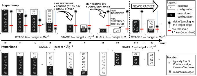
Figure 1: Search methodologies of HJ (top) and HB (bottom). The figure illustrates the 3 key mechanisms of HJ: i) skipping HB stages based on a risk model; ii) determining the order in which configurations are test so as to minimize the risk of future jumps (this is depicted in the figure through the different set of configurations explored by each approach); iii) dynamically updating the risk threshold based on the quality of the current incumbent.

• Expected Accuracy Reduction (EAR) — a novel modelling technique to predict the risk of jumping. The EAR exploits the model’s uncertainty in predicting the quality of untested configurations as a basis to estimate the expected reduction in the accuracy between (i) the best configuration included in the stage reached after a jump and (ii) the best configuration discarded due to the jump.

• A criterion for selecting the configurations to include in the HB stage targeted by a jump, which aims to minimize the jump’s risk. This is a combinatorial problem, which we tackle via a lightweight heuristic that has logarithmic complexity with respect to the number of configurations in the target stage of the jump.

• A method for prioritizing the testing of configurations that aims to promote future jumps, by favouring the sampling of configurations that are expected to yield the highest risk reduction for future jumps.

We conduct an ablation study that sheds light on the contributions of the various mechanisms of HJ on its performance, and compare HJ with a number of state-of-the-art optimizers (Li et al. 2018; Klein et al. 2017; Snoek et al. 2012; Falkner et al. 2018; Li et al. 2020) on both hyper-parameter optimization and neural architecture search (Dong et al. 2021) problems, for sequential and parallel deployments. We show that HJ provides up to over one-order of magnitude speed-ups on deep-learning and kernel-based learning problems.

2 Related Work

Existing hyper-parameter techniques can be coarsely classified along two dimensions: i) whether they use model-free or model-based approaches; ii) whether they exploit solely high-fidelity evaluations or also multi-fidelity ones.

As already mentioned, HB is arguably one of the most prominent model-free approaches. Its random nature, combined with its SH-based search algorithm, makes it not only provably robust, but also efficiently parallelizable (Li et al. 2018; Falkner et al. 2018; Li et al. 2020) and, overall, very competitive and lightweight.

As for the model-based approaches, recent literature on hyper-parameter optimization has been dominated by Bayesian Optimization (BO) (Brochu et al. 2010) methods. BO relies on modelling techniques (e.g., Gaussian Processes (Rasmussen and Williams 2006), Random Forests (Breiman 2001) or Tree Parzen Estimator (TPE) (Bergstra et al. 2011)) to build a surrogate model of the function $f:\mathcal{X}\rightarrow\mathbb{R}$ to be optimized. The surrogate model is then used to guide the selection of the configurations to test via an acquisition function that tackles the exploration-exploitation dilemma. A common acquisition function is the Expected Improvement (EI) (Mockus et al. 1978), which exploits information of the model’s uncertainty on an untested configuration $c$ to estimate by how much $c$ is expected to improve over the current incumbent.

SMAC (Hutter et al. 2011) and MTBO (Swersky et al. 2013) were probably the first to adapt the BO framework to take advantage of low-fidelity evaluations, obtained using training sets of smaller dimensions. This idea was extended in Fabolas (Klein et al. 2017), whose acquisition function factors in the trade-off between the cost of testing a configuration and the knowledge it may reveal about the optimum. A related body of work (Swersky et al. 2014; Domhan et al. 2015; Dai et al. 2019; Golovin et al. 2017; Takeno et al. 2020; Kandasamy et al. 2016; Sen et al. 2018; Poloczek et al. 2017; Song et al. 2019) uses models (typically GPs) to predict the loss of neural networks as a function of both the hyper-parameters and the training iterations. Models are then used to extrapolate the full-training loss and cancel under-performing training runs.

From a methodological perspective, the fundamental difference between HJ and this body of model-based works lies in the type of problems that are addressed by their modelling techniques. Since HJ exploits HB’s search strategy, the models employed in HJ are meant to address a different problem than the above mentioned model-based approaches, namely quantifying the risk of discarding high quality configurations among the ones currently being tested in the current HB’s stage. In other words, HJ’s models are used to reason on a relatively small search space, i.e., the configurations in the current stage. Conversely, the previously mentioned approaches, which do not take advantage of HB’s search algorithm, employ models to estimate configuration’s quality across the whole search space. Further, the modelling techniques used in some of these works (Klein et al. 2017) require computationally expensive implementations, which can impose significant overhead especially when the cost of evaluating configurations is relatively cheap, e.g., when using low-fidelity observations (see Sec. 4).

By taking advantage of the (theoretically provable) robustness of HB, which HJ accelerates in a risk-aware fashion via model-driven techniques, we argue that HJ fuses the best of both worlds: it preserves HB’s robustness (see Sec. 3.3), while accelerating it by more than one order of magnitude via the use of lightweight, yet effective, modelling techniques (as we will show experimentally in Sec. 4).

The works more closely related to HJ are recent approaches, e.g., (Falkner et al. 2018; Wang et al. 2018; Bertrand et al. 2017) that extend HB with BO, or evolutionary search (Awad et al. 2021), to warm start it, i.e., to select (a fraction of) the configurations to include in a new HB bracket. This mechanism is complementary to the key novel idea exploited by HJ to accelerate HB, i.e., short-cutting the SH process by skipping to later SH stages in low risk scenarios. In fact, HJ incorporates a BO-based warm starting mechanism and it would be straightforward to incorporate alternative approaches (e.g., based on evolutionary search (Awad et al. 2021)). Also, when compared with BOHB (Falkner et al. 2018), which warm starts HB via BO, HJ provides more than one order of magnitude speed-ups.

Recently, ASHA (Li et al. 2020) proposed an optimized parallelization strategy for HB that aims at avoiding struggling effects. In Section 3.4 we discuss how HJ’s approach could be applied to ASHA. Further, our experimental study shows that HJ (despite using HB’s original parallelization scheme) still signficantly outperforms ASHA.

Algorithm 1 Pseudo-code for a HJ bracket consisting of $S$ stages, with budget $b$ for the initial stage.

1:  Set$\langle$Config$\rangle$ $C$ = get_configs_for_bracket() $\triangleright$ Model-driven bracket warmstart (Suppl. Mat Sec. 6)

2:  Set$\langle$Config$\rangle$ T = $\emptyset$; Set$\langle$Config$\rangle$U = $C$; $\triangleright$ T and U contain the tested/untested configs, resp.

3:  for $s\in\{0,\ldots,S-1\}$ do $\triangleright$ s denotes the current stage

4:     bool jump = false;

5:     while $U\neq\emptyset$ do $\triangleright$ Test configs. in curr. stage, or jump to a future stage

6:        $\langle$target, $\mathcal{S}\rangle$ = evaluate_jump_risk($s$, T, U) $\triangleright$ HJ risk-analysis (Sec. 3.1)

7:        if target $\neq s$ then $\triangleright$ Jump to target stage

8:           $s$ = target; T = U = $\emptyset$; $C$ = $\mathcal{S}$ ; jump = true; break;

9:        else

10:           c = next_conf_to_test(U, T, $s$); $\triangleright$ Next selected config. minimizes future risk (Sec. 3.2)

11:           acc = evaluate_config(c,$b\eta^{s}$) $\triangleright$ Measure config. c with budget $b\eta^{s}$ and return its accuracy

12:           T = T $\cup~{}\{c\}$; U = U $\setminus$ {c}

13:           update_model($\langle c,b\eta^{s},acc\rangle$)

14:        end if

15:     end while

16:     if $\neg$jump then $\triangleright$ Use HB’s policy if HJ did not trigger a jump by the end of the stage

17:        U = $C$ = topK($C$, $|C|\eta^{-1}$) $\triangleright$ test top $1/|\eta|$% configs. in next stage

18:     end if

19:  end for

3 HyperJump

As already mentioned, an HB bracket is composed of up to $S_{max}$ stages, where $S_{max}=\lfloor log_{\eta}(R)\rfloor$. $R$ is the maximum “budget” allocated to the evaluation of a hyper-parameter configuration and $\eta$ is an exponential factor (typically 2 or 3) that controls the increase/decrease of the allocated budget/number of tested configurations in two consecutive stages of the same bracket.

The pseudo-code in Alg. 1 overviews the various mechanisms employed by HJ to accelerate a single HB bracket composed of $S<S_{max}$ stages. The bracket’s initial stage allocates a budget $b$, where $b=R\eta^{-(S-1)}$, as prescribed by HB. HJ leverages two main mechanisms to accelerate the execution of a HB bracket, which are encapsulated in the functions evaluate_jump_risk and next_config_to_test.

evaluate_jump_risk is executed within HJ’s inner loop (Alg. 1, line 6), to decide whether to stop testing configurations in the current stage and jump to a later stage. This function takes as input the current stage, $s$, and the configurations already and still to be tested, $T$ and $U$. It returns the pair $\langle target,\mathcal{S}\rangle$ where $target$ denotes the stage to jump to (in which case $target\neq s$) and $\mathcal{S}$ the selected configurations for the target stage. We detail this function in Sec. 3.1.

If the risk of jumping is deemed too high, HJ continues testing configurations in the current stage. Unlike HB, which uses a random order of exploration, HJ prioritizes the order of exploration via the next_conf_to_test function (Alg. 1, line 10). This function seeks to identify a configuration whose evaluation will lead to a large reduction of the risk of jumping, so as to favour earlier jumps and enhance the efficiency of HJ. We discuss how we implement this function in Sec. 3.2. After testing configuration $c$ in budget $b\eta^{s}$ and measuring its accuracy $acc$, we update the models used to predict the accuracy of untested configurations (with different budgets).

Finally, get_configs_for_bracket (Alg. 1, line 1) encapsulates the model-driven warm starting procedure, which selects the configurations to include in a new bracket. As mentioned, this idea was already explored in prior works, e.g., BOHB (Falkner et al. 2018), so we detail its implementation in the supplemental material (Mendes et al. 2021), along with the description of other previously published optimizations that we incorporated in HJ (e.g., resuming training of configurations previously on smaller budgets (Swersky et al. 2014)). The supplemental material includes also an analysis of HJ’s algorithmic complexity (Sec. 7).

3.1 Deciding whether to jump

We address the problem of deciding whether to adopt HB’s default policy or skip some, or even all, of the future stages of the current bracket by decomposing it into three simpler sub-problems: 1) modelling the risk of jumping from the current stage to the next stage while retaining an arbitrary subset $\mathcal{S}$ of the configurations $C$ in the current stage; 2) identifying “good” candidates for the subset of configurations to retain after a jump from stage $s$ to stage $s+1$, i.e., configurations that, if included in the target stage of the jump, reduce the risk of jumping; 3) generalizing the risk modelling to jumps that skip an arbitrary number of stages. Next, we discuss how we address each sub-problem.

Firstly, HJ’s risk analysis methodology relies on GP-based models to estimate the accuracy of a configuration $c$ in a given budget. As in recent works, e.g., (Klein et al. 2017, 2020; Mendes et al. 2020), we include in the feature space of the GP models not only the hyper-parameters’ space, but also the budget (so as to enable inter-budget extrapolation). Further, analogously to, e.g., (Klein et al. 2017; Mendes et al. 2020), we employ a custom kernel that encodes the expectation that the loss function has an exponential decay with larger budgets along with a generic Matérn 5/2 kernel that is used to capture relations among the hyper-parameters.

1. Modelling the risk of 1-hop jumps.

Let us start by discussing how we model the risk of jumping from a source (current) stage $s$ to a target stage $t$ that is the immediate successor of $s$ ($t\!\!=\!\!s\!+\!1$). Consider $C$ the configurations in $s$; $T$ and $U$ the tested/untested configurations in $s$, resp., and $\mathcal{S}$ and $\mathcal{D}$ the subset of configurations in $C$ that are selected/discarded, resp., when jumping to stage $t$. Our modelling approach is based on the observation that short-cutting HB’s search process and jumping to the next stage exposes the risk of discarding the configuration that achieves maximum accuracy in the current stage (and that may turn out to improve the current incumbent when tested in full-budget). This risk can be modelled as the difference between two random variables defined as the maximum accuracy of the configurations in the set of discarded $\mathcal{D}$ and selected $\mathcal{S}$ configurations in stage $s$ and budget $b\eta^{s}$, resp.:

$$\mathcal{A}^{\mathcal{D}}_{s}=\underset{c\in\mathcal{D}}{\text{max}}~{}A(c,b\eta^{s}),~{}~{}~{}\mathcal{A}^{\mathcal{S}}_{s}=\underset{c\in\mathcal{S}}{\text{max}}~{}A(c,b\eta^{s})$$

having denoted with $A(c_{i},b\eta^{s})$ the accuracy of a configuration $c_{i}$ using budget $b\eta^{s}$. From a mathematical standpoint, we only require $\mathcal{A}$ to be finite, so that the maximum and difference operators are defined. So, one may use arbitrary accuracy metrics as long as they match this assumption, e.g., unbounded but finite metrics like negative log likelihood.

One can then quantify the “absolute” risk of a jump from stage $s$ to stage $s+1$, which we call Expected Accuracy Reduction (EAR) (Eq. (1)), as the expected value of the difference between these two variables, restricted to the scenarios in which configurations with higher accuracy are discarded due to jumping (i.e., $\mathcal{A}^{\mathcal{D}}-\mathcal{A}^{\mathcal{S}}>0$):

$$EAR_{s}^{s+1}(\mathcal{D},\mathcal{S}) \mkern 1.5mu{=}\mkern 1.5mu\int_{-\infty}^{+\infty}\!\!P\!\left(\mathcal{A}^{\mathcal{D}}_{s}\!-\!\mathcal{A}^{\mathcal{S}}_{s}\mkern 1.5mu{=}\mkern 1.5mux\right)\text{max}\{\mathcal{A}^{\mathcal{D}}_{s}\!-\!\mathcal{A}^{\mathcal{S}}_{s},0\}dx$$ (1)

$$\mkern 1.5mu{=}\mkern 1.5mu\int_{0}^{+\infty}\!\!xP\left(\mathcal{A}^{\mathcal{D}}_{s}\!-\!\mathcal{A}^{\mathcal{S}}_{s}\mkern 1.5mu{=}\mkern 1.5mux\right)dx$$

The EAR is computed as follows. The configurations in $\mathcal{D}$ and $\mathcal{S}$ are either untested or already tested. In the former case, we model their accuracy via a Gaussian distribution (given by the GP predictors); in the latter case, we model their accuracy either as a Dirac function (assuming noise-free measurements, which is HJ’s default policy) or via a Gaussian distribution (whose variance can be used to model noisy measurements). In any case, the PDF and CDF of $\mathcal{A}^{\mathcal{D}}$ and $\mathcal{A}^{\mathcal{S}}$ can be computed in closed form. Yet, computing the difference between these two random variables requires solving a convolution that cannot be determined analytically. Fortunately, both this convolution and the outer integral in Eq. (1) can be computed in a few msecs using open source numerical libraries (Sec. 4). Additional details on the EAR’s computation are provided in the supplemental material.

Next, we introduce the rEAR (relative EAR), which is obtained by normalizing the EAR by the loss of the current incumbent, noted $l^{*}$: $rEAR_{s}^{s+1}(\mathcal{D},\mathcal{S})={EAR_{s}^{s+1}(\mathcal{D},\mathcal{S})}/{l^{*}}$. The rEAR estimates the “relative” risk of a jump and can be interpreted as the percentage of the maximum potential for improvement that is expected to be sacrificed by a jump. In HJ, we consider a jump “safe” if its corresponding rEAR is below a threshold $\lambda$, whose default value we set to $10\%$. As we show in the supplemental material, in practical settings, HJ has robust performances for a large range of (reasonable) values of $\lambda$. One advantage of using the rEAR, instead of the EAR as risk metric is that the rEAR allows for adapting the risk propensity of HJ’s logic, making HJ progressively less risk prone as the optimization process evolves and new incumbents are found.

Algorithm 2 Pseudo-code of the logic used to determine the sets of configurations to consider when jumping from stage $s$ to stage $s+1$ (function get_candidates_for_$\mathcal{S}$())

1:  Set$\langle$Set$\langle$Config$\rangle\rangle$ get_candidates_for_$\mathcal{S}$(Set$\langle$Config$\rangle$ Tested, Set$\langle$Config$\rangle$ Untested)

2:  Set$\langle$Set$\langle$Config$\rangle\rangle O\leftarrow\emptyset$ $\triangleright$ Set of selected safest sets to be returned

3:  Set$\langle$Config$\rangle$ $C\leftarrow$ Tested $\cup$ Untested $\triangleright$ $C$ stores all the configs in current stage

4:  Set$\langle$Config$\rangle$ $\mathcal{K}\leftarrow C.sortByAccuracy().getTop(|C|/\eta)$

5:  $\triangleright$ $\mathcal{K}$ stores the configs. with best (pred. or measured) accuracy

6:  Set$\langle$Config$\rangle$ $E\leftarrow C\setminus\mathcal{K}$

7:  $\triangleright$ $E$ stores the configs. with worse (pred. or measured) accuracy

8:  $O.add(\mathcal{K})$ $\triangleright$ Set $\mathcal{K}$ is one of the $1+2\lfloor log_{\eta}|\mathcal{K}|\rfloor$ recommended sets

9:  $\triangleright$ Generate sets based on accuracy

10:  for $i$ in $[1\leq i\leq\lfloor log_{\eta}|\mathcal{K}|\rfloor$ do

11:     Set $X\leftarrow clone(\mathcal{K})$

12:     $\triangleright$ Remove from $K$ the $\mathcal{|K|}/\eta^{i}$ configurations with worse accuracy…

13:     $X.removeBottom(\mathcal{|K|}/\eta^{i})$

14:     $\triangleright$ …and add the $\mathcal{|K|}/\eta^{i}$ configurations with best accuracy from $C\setminus\mathcal{K}$

15:     $X.add(E.getTop(\mathcal{|K|}/\eta^{i}))$

16:     $O.add(X)$

17:  end for

18:  $\mathcal{K}\leftarrow\mathcal{K}.sortByLCB()$ $\triangleright$ sort configs in $\mathcal{K}$ by LCB

19:  $E\leftarrow E.sortByUCB()$ $\triangleright$ sort configs in $E$ by UCB

20:  $\triangleright$ Generate sets based on lower and upper confidence bounds

21:  for $i$ in $[1\leq i\leq\lfloor log_{\eta}|\mathcal{K}|\rfloor$ do

22:     Set $X\leftarrow clone(\mathcal{K})$

23:     $\triangleright$ Remove from $K$ the $|K|/\eta^{i}$ configurations with worse LCB

24:     $X.removeBottom(\mathcal{|K|}/\eta^{i})$

25:     $\triangleright$ …and add the $|\mathcal{K}|/\eta^{i}$ configurations with best UCB from $C\setminus\mathcal{K}$

26:     $X.add(E.getTop(|\mathcal{K}|/\eta^{i}))$

27:     $O.add(X)$

28:  end for

29:  return $O$

2. Identifying the safest set of configurations for a jump.

Determining the safest subset of configurations to include when jumping to the next stage via naive, enumerative methods would have prohibitive costs, as it would require evaluating the rEAR for all possible subsets $\mathcal{S}$ of size $|C|/\eta$ of the configurations in the current stage $s$. For instance, assuming $\eta\!=\!3$, $|C|\!=\!81$ and that less than half of the configurations in $C$ were tested, the number of distinct target sets for a jump of a single stage is $\binom{81}{27}\approx$ 2E21.

We tackle this problem by introducing an efficient, model-driven heuristic that recommends a total of 1+2$\lfloor$log${}_{\eta}|\mathcal{S}|\rfloor$ candidates for $\mathcal{S}$ (see Alg. 2). The first candidate set evaluated by HJ, denoted $\mathcal{K}$, is obtained by considering the top $|\mathcal{S}|$ configurations, ranked based on their actual or predicted accuracy depending on whether they have already been tested or not (line 4).

Next, using $\mathcal{K}$ as a template, we generate $\lfloor$log${}_{\eta}|\mathcal{S}|\rfloor$ alternative sets by replacing the worst $|\mathcal{S}|/\eta^{i}$ (1$\leq i\leq\lfloor$log${}_{\eta}|\mathcal{S}|\rfloor$) configurations in $\mathcal{K}$ with the next best configurations in $C\setminus\mathcal{K}$, ranked based on their (predicted/measured) accuracy (lines 10-17). Next (lines 21-28), we generate $\lfloor$log${}_{\eta}|\mathcal{S}|\rfloor$ alternative candidate sets by exploiting model uncertainty as follows: we identify the worst $|\mathcal{S}|/\eta^{i}$ configurations in $\mathcal{K}$, ranked according to their lower confidence bound, and replace them with the configurations in $C\setminus\mathcal{K}$ that have the highest confidence (we use a confidence bound of 90%). Intuitively, this way we remove from the reference set $\mathcal{K}$ the configurations that are likely to have lower accuracy if the model overestimated their mean. These are replaced by the configurations that, although having lower (average) predicted accuracy, are prone to achieve high accuracy, given the model’s uncertainty. Refer to the supplemental material for diagrams illustrating the behavior of this algorithm.

3. Generalizing to multi-hop jumps.

Alg. 3 shows how to compute the rEAR of a jump that skips $j\!>\!1$ stages from the current stage $s$. This is done in an iterative fashion by computing the rEAR for jumps from stage $s+i$ to stage $s+i+1$ ($i\in[1,j-1]$) and accumulating the corresponding rEARs to yield the rEAR of the jump.

At each iteration, the candidate sets for the set $\mathcal{S}$ of configurations to be retained after the jump are obtained via the get_candidates_for_$\mathcal{S}$ function. Among these 1+2$\lfloor$log${}_{\eta}|\mathcal{S}|\rfloor$ candidate sets, the one with minimum risk is identified. The process is repeated replacing $C$ with the candidate set that minimizes the risk of the current jump (line 11), until $\lambda$ is exceeded, thus seeking to maximize the “jump length”, i.e., the number of stages that can be safely skipped. As such, the computation of the risk of a jump from a stage with $|C|$ configurations and that skips $j\!>\!1$ stages requires $\mathcal{O}(j(1+log_{\eta}|C|/~{}\eta))$ rEAR evaluations. This ensures the scalability of HJ’s risk analysis methodology even when considering jumps that can skip a large number of stages.

Algorithm 3 Pseudo-code for the Evaluate_Jump_Risk function.

1:  $\langle$int s, Set$\langle$Config$\rangle\mathcal{S}\rangle$ Evaluate_Jump_Risk(int s, Set$\langle$Config$\rangle$ Tested, Set$\langle$Config$\rangle$ Untested)

2:  rEAR = 0; $\mathcal{S}$ = $\emptyset$; $C$ = Tested $\cup$ Untested.

3:  while s $<$ S do $\triangleright$ $S$: maximum number of stages

4:     Set$\langle$Set$\langle$Config$\rangle\rangle$ candidates = get_candidates_for_$\mathcal{S}$(Tested, Untested)

5:     minRisk = min${}_{\mathcal{X}\in\text{candidates}}$ rEAR${}_{s}^{s+1}(\mathcal{X},C\setminus\mathcal{X})$

6:     $\mathcal{S}=\text{argmin}_{\mathcal{X}\in\text{candidates}}$ rEAR${}_{s}^{s+1}(\mathcal{X},C\setminus\mathcal{X})$ $\triangleright$ $\mathcal{S}$: Set that minimizes the risk

7:     if rEAR + minRisk $>\lambda$ then

8:        return $\langle$ s , $\mathcal{S}\rangle$ $\triangleright$ Return the target stage and the set with selected configs.

9:     else $\triangleright$ Try to extend the jump by one hop

10:        rEAR += minRisk; s++

11:        $C$ = Untested = $\mathcal{S}$; Tested = $\emptyset$

12:     end if

13:  end while

14:  return $\langle$ s, $\emptyset\rangle$ $\triangleright$ Jump all stages in the current bracket and start a new bracket

3.2 Reducing the risk of jumping by prioritizing the evaluation order of configurations

HJ also uses a model-based approach to determine in which order to evaluate the configurations of a stage. This mechanism aims to enhance HJ’s efficiency by prioritizing the evaluation of configurations that are expected to yield the largest reduction of risk for future jumps. The literature on look-ahead non-myopic BO (Yue and Kontar 2020; Casimiro et al. 2020; Lam et al. 2016; Lam and Willcox 2017) has already investigated several techniques aimed at predicting the impact of future exploration steps on model-driven optimizers. These approaches often impose large computational overheads, due to the need to perform expensive “simulations”, e.g., retraining the models to simulate alternative evaluation outcomes, and to their ambition to maximize long-term rewards (in contrast to the greedy nature of typical BO approaches).

Motivated by our design goal of keeping HJ efficient and scalable, we opted for a greedy heuristic that allows for estimating the impact of evaluating an untested configuration in a light-weight fashion, e.g., avoiding retraining the GP models. More in detail, we simulate the evaluation of an untested configuration $c$ by including $c$ in the set of tested configurations and considering its accuracy to be the one predicted via the GP model’s posterior mean. Next, we execute the Evaluate_Jump_Risk function to obtain the updated risk of jumping and the corresponding target stage. We repeat this procedure for all the untested configurations in the stage, and select, as the next to test, the one that enables the longest safest jump (determined via the Evaluate_Jump_Risk function). The pseudo-code of this mechanism can be found in the supplemental material.

3.3 Preserving HyperBand’s Robustness

An appealing theoretical property of HB is that its exploration policy is guaranteed to be at most a constant factor slower than random search. In order to preserve this property, HJ exploits two mechanisms: i) with probability $p_{NJ}$ HJ is forced not to jump and abide by the original SH/HB logic; ii) when selecting the configurations to include in a bracket, a fraction $p_{U}$ is selected uniformly at random (as in HB) and not using the model. The former mechanism ensures that, regardless of how model mispredictions affect HJ’s policy, there exists a non-null probability that HJ will not deviate from HB’s policy (by jumping) in any of the brackets that it executes. The latter mechanism, originally proposed in BOHB (Falkner et al. 2018), ensures that, independently of the model’s behavior, every configuration has a non-null probability of being included in a bracket. We adopt as default value for $p_{U}$ the same used by BOHB, i.e., 0.3, and use the same value also for $p_{NJ}$.

3.4 Parallelizing HyperJump

Existing approaches for parallelizing HB can be classified as synchronous or asynchronous. In synchronous approaches (Li et al. 2018; Falkner et al. 2018), the size of the stages abides by HB’s rules and parallelization can be achieved at the level of a HB’s stage, bracket, and iteration. Conversely, asynchronous methods (ASHA (Li et al. 2020) or Ray Tune (Liaw et al. 2018)) consider a single logical bracket that promotes a configuration $c$ to the next stage iff $c$ is in the top $\eta^{-1}$ configurations tested in the current stage.

HJ can be straightforwardly parallelized using synchronous strategies. If parallelization is pursued at the level of brackets or iterations, each worker simply runs an independent instance of HJ that shares the same model and training set (so to share the knowledge acquired by the parallel HJ instances). When parallelizing the testing of the configurations in the same stage, as soon as a worker completes the testing of a configuration, the model can be updated and the risk of jumping computed. If a jump is performed, the workers that are still evaluating configurations in the current stage can either be immediately interrupted or allowed to complete their current evaluation. In our implementation, we opted for the former option, which has the advantage of maximizing the workers that are immediately available for testing configurations in the stage targeted by the jump.

In more detail, our implementation adopts the same parallelization strategy of BOHB, i.e., parallelizing by stage and activating a new parallel bracket in the presence of idle workers, with one exception. We prevent starting a new parallel bracket if there are idle workers during the first bracket. This, in fact, would reduce the available computational resources to complete the first bracket and, consequently, lead to a likely increase of the latency to recommend the first incumbent (i.e., to test a full budget configuration).

Investigating how to employ HJ in combination with asynchronous versions of HB is out of the scope of this paper. Yet, we argue that the key ideas at the basis of HJ could still be applied in this context, opening up an interesting line of future research. For instance, in ASHA, one could use a model-based approach, similar to the one employed by HJ, to: (i) promote “prematurely” configurations that the model predicts to be promising; or (ii) use the model to delay promotions of less promising configurations.

4 Evaluation

This section evaluates HJ both in terms of the quality of the recommended configurations and of its optimization time. We compare HJ against 6 state-of-the-art optimizers using 9 benchmarks and considering both sequential and parallel deployments. We also perform an ablation study to dive into the performance of HJ’s different components.

Benchmarks.

Our first benchmark is the NATS-Bench (Dong et al. 2021), which optimizes the topology of a NN, fixing the number of layers and hyper-parameters, using 2 different data sets (ImageNet-16-120 (Russakovsky et al. 2015) and Cifar100). The search space encompasses 6 dimensions (each one represents a connection between two layers and have 5 possible topologies). This benchmark contains an exhaustive evaluation of all possible 15625 configurations.

We also use LIBSVM (Chang and Lin 2011) on the Covertype data set (Dua and Graff 2017), which we sub-sampled by $\approx 5\times$ due to time and hardware constraints. The considered hyper-parameters are the kernel (linear, polynomial, RBF, and sigmoid), $\gamma$, and C. In this case, we could not exhaustively explore off-line the hyper-parameter space, so the optimum is unknown.

Additional details on the above benchmarks can be found in the supplemental material. Further, the supplemental material reports additional results using 2 alternative data-sets (Cifar10 (Krizhevsky and Hinton 2009), 2017 CCF-BDCI (Ronneberger et al. 2015), and MNIST (Deng 2012)) and different models (such as Light UNET (Ronneberger et al. 2015), CNN).

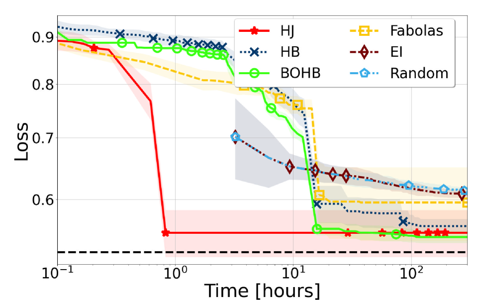
(a) NATS ImageNet (1 worker)

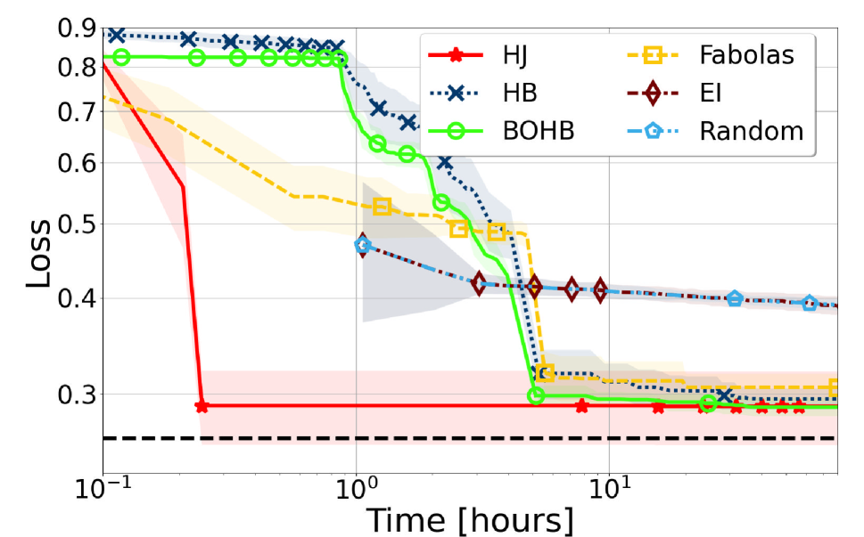
(b) NATS Cifar100 (1 worker)

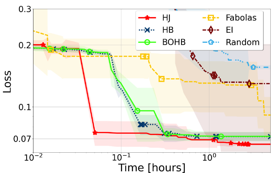
(c) SVM Covertype (1 worker)

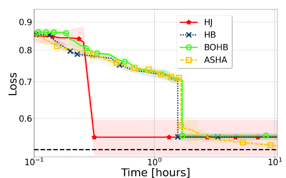
(d) NATS ImageNet (32 workers)

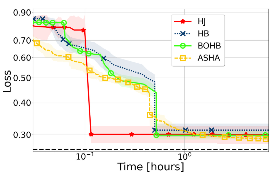
(e) NATS Cifar100 (32 workers)

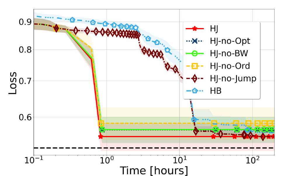
(f) Ablation Study ImageNet (1 worker)

Figure 2: Comparison of HJ against other state-of-the-art optimizers in sequential and parallel deployments. Figure (f) reports an ablation study. The dashed horizontal line indicates the optimum (when it is known). Additional results are reported in the supplementary material.

Baselines and experimental setup.

We compare HJ against six optimizers: HB, BOHB, ASHA, Fabolas, standard BO with EI, and Random Search (RS). The last two techniques (EI and RS) evaluate configurations only with the full-budget. The implementation of HJ extends the publicly available code of BOHB, which also provides an implementation of HB. ASHA was implemented via the Ray-Tune framework (Liaw et al. 2018). Fabolas was evaluated using its publicly available implementation.

We use the default parameters of BOHB and Fabolas. Similarly to HB, we set the parameter $\eta$ to 3, and for fairness, when comparing HJ, HB, BOHB, and ASHA, we configure them to use the same $\eta$ value. We use the default value of 10% for the threshold $\lambda$ for HJ and include in the supplemental material a study on the sensitivity to the tuning of $\lambda$. We use number of epochs as budget for NATS and training set size for LIBSVM. The reported results represent the average of 30 independent runs. We have made available the implementation of HJ and the benchmarks used .

Sequential deployment.

Figure 2 reports the average loss (i.e., the test error rate) and corresponding standard deviation in the shaded areas as a function of the wall clock time (i.e., training and recommendation time). We start by analyzing the plots in the first rows, which refer to a sequential deployment scenario, i.e., a single worker is available for evaluating configurations. We do not include ASHA in this study, since ASHA is designed for parallel deployments.

In all the benchmarks, HJ provides significant speed-ups with respect to all the baselines to identify near optimal configurations. The largest speed-ups for recommending near optimal solutions are achieved with ImageNet and Cifar100, where the gains of HJ w.r.t. the best baseline are around 20$\times$ to 32$\times$, respectively. Using SVM, the HJ speed-ups to identify good quality configuration (i.e., loss around 0.08) are approx. 7$\times$ w.r.t. to the most competitive baselines, namely HB and BOHB. Note that HJ outperforms these two baselines also in the final stages of the optimization: HJ’s final loss is 0.066$\pm$8.9E-4, whereas HB and BOHB’s final losses are 0.072$\pm$3.6E-3 and 0.72$\pm$3.5E-3, respectively.

In our benchmarks, BOHB provides marginal (ImageNet and Cifar100) or no (SVM) benefits when compared to HB. As shown in the supplemental material (Section 13), this is imputable to the limited accuracy of the modelling approach used by BOHB (based on TPE and on a model per budget) which, albeit fast, is not very effective in identifying high quality configurations to include in a new bracket. Fabolas’ performance, conversely, is hindered by its large recommendation times, which are already on the order of a few minutes in the early stages of the optimization and grow more than linearly: consequently, Fabolas suffers from large overheads especially with benchmarks that have shorter training times, such as SVM. Lastly, the limitations of EI, which only uses full-budget sampling, are notably clear with SVM. Here, training times grow more than linearly with the training set size (which is the budget used by the multi-fidelity optimizers), thus amplifying the speed-ups achievable by using low-fidelity observations w.r.t. the other benchmarks.

Ablation study.

Figure 2(f) shows the result of an ablation study aimed at quantifying the contributions of the various mechanisms employed by HJ. We report the performance achieved on ImageNet by four HJ variants obtained by disabling each of the following mechanisms: (i) the jumping logic (HJ-no-Jump) (see supplemental material). (ii) prioritizing the evaluation order of configurations (HJ-no-Ord); (iii) the pause-resume training(Swersky et al. 2014) and opportunistic evaluation optimizations (Liaw et al. 2018), see Sec. 6 of the supplemental material (HJ-no-Opt); (iv) the bracket warm-starting (Wang et al. 2018) logic, see Sec. 6 of the supplemental material (HJ-no-BW).

We include in the plot also HB, which can be regarded as a variant of HJ from which we disabled all of the above mechanisms. This data shows that the last two of these mechanisms, which correspond to previously published optimizations of HB, have a similar and small impact on the performance of HJ. Conversely, the largest performance penalty is observed when disabling jumping. This confirms that this mechanism is indeed the one that contributes the most to HJ’s efficiency. Finally, this plot also shows the relevance of the heuristics that determines the order of configuration testing in a bracket described in Section 3.2.

Parallel Deployment.

Figures 2(d) and 2(e) report the results when using a pool of 32 workers with NATS-Bench with ImageNet and Cifar100. The supplemental material includes the plots for the other benchmarks, as well as for a scenario with 8 workers. These data show that HJ achieves gains similar to the ones previously observed compared to HB and BOHB. With respect to the other baselines (and to HJ), ASHA adopts a more efficient parallelization scheme (see Section 3.4). Thus, the gains of HJ w.r.t. ASHA are slightly reduced. Still, HJ achieves speed-ups of up to approximately 6$\times$ to recommend near-optimal configurations. This confirms HJ’s competitiveness even when compared with HB variants that use optimized parallelization schemes.

Recommendation overhead.

We conclude by reporting experimental data regarding the computational overhead incurred by HJ to recommend the next configuration to test. The average recommendation time for HJ across all benchmarks is approx. 1.08 secs. This time includes model training, determining whether to jump and the next configuration to test in the current stage, and, overall, confirms the computational efficiency of the proposed approach.

5 Conclusions

This paper introduced HyperJump, a new approach that complements HyperBand’s robust search strategy and accelerates it by skipping low risk evaluations. HJ’s efficiency hinges on the synergistic use of several innovative risk modelling techniques and of a number of pragmatic optimizations. We show that HJ provides over one-order of magnitude speed-ups on a variety of kernel-based and deep learning problems when compared to HB as well as to a number of state-of-the-art optimizers.

See pages - of supple_hyperjump_aaai23.pdf

References

- Awad et al. (2021) Awad, N. H.; Mallik, N.; and Hutter, F. 2021. DEHB: Evolutionary Hyberband for Scalable, Robust and Efficient Hyperparameter Optimization. In Zhou, Z., ed., Proceedings of the Thirtieth International Joint Conference on Artificial Intelligence, IJCAI 2021, Virtual Event / Montreal, Canada, 19-27 August 2021, 2147–2153. ijcai.org.
- Bergstra et al. (2011) Bergstra, J.; Bardenet, R.; Bengio, Y.; and Kégl, B. 2011. Algorithms for Hyper-Parameter Optimization. In Advances in Neural Information Processing Systems, volume 24, 2546–2554. Curran Associates, Inc.
- Bertrand et al. (2017) Bertrand, H.; Ardon, R.; Perrot, M.; and Bloch, I. 2017. Hyperparameter optimization of deep neural networks: combining Hperband with Bayesian model selection. In Proceedings of Conférence sur l’Apprentissage Automatique.
- Breiman (2001) Breiman, L. 2001. Random Forests. Machine Learning, 45(1).
- Brochu et al. (2010) Brochu, E.; Cora, V. M.; and de Freitas, N. 2010. A Tutorial on Bayesian Optimization of Expensive Cost Functions, with Application to Active User Modeling and Hierarchical Reinforcement Learning. Technical Report arXiv:1012.2599.
- Casimiro et al. (2020) Casimiro, M.; Didona, D.; Romano, P.; Rodrigues, L.; Zwanepoel, W.; and Garlan, D. 2020. Lynceus: Cost-efficient Tuning and Provisioning of Data Analytic Jobs. In Proceedings 20th IEEE International Conference on Distributed Computing Systems.
- Chang and Lin (2011) Chang, C.-C.; and Lin, C.-J. 2011. LIBSVM: A Library for Support Vector Machines. ACM Transactions on Intelligent Systems and Technology, 2.
- Dai et al. (2019) Dai, Z.; Yu, H.; Low, B. K. H.; and Jaillet, P. 2019. Bayesian Optimization Meets Bayesian Optimal Stopping. In Proceedings of the 36th International Conference on Machine Learning, volume 97.
- Deng (2012) Deng, L. 2012. The MNIST database of handwritten digit images for machine learning research [Best of the Web]. In IEEE Signal Processing Magazine, volume 29. IEEE.
- Domhan et al. (2015) Domhan, T.; Springenberg, J. T.; and Hutter, F. 2015. Speeding up Automatic Hyperparameter Optimization of Deep Neural Networks by Extrapolation of Learning Curves. In Proceedings of the 24th International Joint Conference on Artificial Intelligence.
- Dong et al. (2021) Dong, X.; Liu, L.; Musial, K.; and Gabrys, B. 2021. NATS-Bench: Benchmarking NAS Algorithms for Architecture Topology and Size. IEEE Transactions on Pattern Analysis and Machine Intelligence (TPAMI). doi:10.1109/TPAMI.2021.3054824.
- Dua and Graff (2017) Dua, D.; and Graff, C. 2017. UCI Machine Learning Repository.
- Falkner et al. (2018) Falkner, S.; Klein, A.; and Hutter, F. 2018. BOHB: Robust and Efficient Hyperparameter Optimization at Scale. In Proceedings of the 35th International Conference on Machine Learning, volume 80.
- Golovin et al. (2017) Golovin, D.; Solnik, B.; Moitra, S.; Kochanski, G.; Karro, J.; and Sculley, D. 2017. Google Vizier: A Service for Black-Box Optimization. In Proceedings of the 23rd ACM SIGKDD International Conference on Knowledge Discovery and Data Mining.
- Hutter et al. (2011) Hutter, F.; Hoos, H. H.; and Leyton-Brown, K. 2011. Sequential Model-Based Optimization for General Algorithm Configuration. In Proceedings of the 5th International Conference on Learning and Intelligent Optimization, 507–523.
- Jamieson and Talwalkar (2016) Jamieson, K.; and Talwalkar, A. 2016. Non-stochastic best arm identification and hyperparameter optimization. In Proceedings of the 19th International Conference on Artificial Intelligence and Statistics.
- Kandasamy et al. (2016) Kandasamy, K.; Dasarathy, G.; Oliva, J. B.; Schneider, J.; and Poczos, B. 2016. Gaussian Process Bandit Optimisation with Multi-fidelity Evaluations. In Lee, D.; Sugiyama, M.; Luxburg, U.; Guyon, I.; and Garnett, R., eds., Advances in Neural Information Processing Systems, volume 29. Curran Associates, Inc.
- Klein et al. (2017) Klein, A.; Falkner, S.; Bartels, S.; Hennig, P.; and Hutter, F. 2017. Fast Bayesian Optimization of Machine Learning Hyperparameters on Large Datasets. In Proceedings of the 20th International Conference on Artificial Intelligence and Statistics, volume 54.
- Klein et al. (2020) Klein, A.; Tiao, L. C.; Lienart, T.; Archambeau, C.; and Seeger, M. 2020. Model-based asynchronous hyperparameter and neural architecture search. arXiv preprint arXiv:2003.10865.
- Krizhevsky and Hinton (2009) Krizhevsky, A.; and Hinton, G. 2009. Learning multiple layers of features from tiny images. Technical report, University of Toronto.
- Lam and Willcox (2017) Lam, R.; and Willcox, K. 2017. Lookahead Bayesian Optimization with Inequality Constraints. In Proceedings of the 31st International Conference on Neural Information Processing Systems.
- Lam et al. (2016) Lam, R. R.; Willcox, K. E.; and Wolpert, D. H. 2016. Bayesian Optimization with a Finite Budget: An Approximate Dynamic Programming Approach. In Proceedings of the 29th Neural Information Processing Systems Conference.
- Li et al. (2018) Li, L.; Jamieson, K.; DeSalvo, G.; Rostamizadeh, A.; and Talwalkar, A. 2018. Hyperband: A novel bandit-based approach to hyperparameter optimization. Journal of Machine Learning Research, 18: 1–52.
- Li et al. (2020) Li, L.; Jamieson, K.; Rostamizadeh, A.; Gonina, E.; Ben-tzur, J.; Hardt, M.; Recht, B.; and Talwalkar, A. 2020. A System for Massively Parallel Hyperparameter Tuning. In Dhillon, I.; Papailiopoulos, D.; and Sze, V., eds., Proceedings of Machine Learning and Systems, volume 2, 230–246.
- Liaw et al. (2018) Liaw, R.; Liang, E.; Nishihara, R.; Moritz, P.; Gonzalez, J. E.; and Stoica, I. 2018. Tune: A Research Platform for Distributed Model Selection and Training. arXiv preprint arXiv:1807.05118.
- Mendes et al. (2020) Mendes, P.; Casimiro, M.; Romano, P.; and Garlan, D. 2020. TrimTuner: Efficient Optimization of Machine Learning Jobs in the Cloud via Sub-Sampling. In 2020 28th International Symposium on Modeling, Analysis, and Simulation of Computer and Telecommunication Systems. IEEE.
- Mendes et al. (2021) Mendes, P.; Casimiro, M.; Romano, P.; and Garlan, D. 2021. HyperJump: Accelerating HyperBand via Risk Modelling. CoRR, abs/2108.02479.
- Mockus et al. (1978) Mockus, J.; Tiesis, V.; and Zilinskas, A. 1978. The Application of Bayesian Methods for Seeking the Extremum. In Toward Global Optimization, volume 2, 117–128. Elsevier.
- Poloczek et al. (2017) Poloczek, M.; Wang, J.; and Frazier, P. 2017. Multi-Information Source Optimization. In Guyon, I.; Luxburg, U. V.; Bengio, S.; Wallach, H.; Fergus, R.; Vishwanathan, S.; and Garnett, R., eds., Advances in Neural Information Processing Systems, volume 30. Curran Associates, Inc.
- Rasmussen and Williams (2006) Rasmussen, C. E.; and Williams, C. K. 2006. Gaussian Processes for Machine Learning. Cambridge, MA, USA: MIT Press.
- Ronneberger et al. (2015) Ronneberger, O.; Fischer, P.; and Brox, T. 2015. U-Net: Convolutional Networks for Biomedical Image Segmentation. In Medical Image Computing and Computer-Assisted Intervention – MICCAI 2015. Springer International Publishing.
- Russakovsky et al. (2015) Russakovsky, O.; Deng, J.; Su, H.; Krause, J.; Satheesh, S.; Ma, S.; Huang, Z.; Karpathy, A.; Khosla, A.; Bernstein, M.; Berg, A. C.; and Fei-Fei, L. 2015. ImageNet Large Scale Visual Recognition Challenge. International Journal of Computer Vision (IJCV), 115(3): 211–252.
- Sen et al. (2018) Sen, R.; Kandasamy, K.; and Shakkottai, S. 2018. Multi-Fidelity Black-Box Optimization with Hierarchical Partitions. In Dy, J.; and Krause, A., eds., Proceedings of the 35th International Conference on Machine Learning, volume 80 of Proceedings of Machine Learning Research, 4538–4547. PMLR.
- Snoek et al. (2012) Snoek, J.; Larochelle, H.; and P. Adams, R. 2012. Practical Bayesian Optimization of Machine Learning Algorithms. In Proceedings of the 25th International Conference on Neural Information Processing Systems, volume 2.
- Song et al. (2019) Song, J.; Chen, Y.; and Yue, Y. 2019. A General Framework for Multi-fidelity Bayesian Optimization with Gaussian Processes. In Chaudhuri, K.; and Sugiyama, M., eds., Proceedings of the Twenty-Second International Conference on Artificial Intelligence and Statistics, volume 89 of Proceedings of Machine Learning Research, 3158–3167. PMLR.
- Swersky et al. (2013) Swersky, K.; Snoek, J.; and Adams, R. P. 2013. Multi-task Bayesian Optimization. In Proceedings of the 26th International Conference on Neural Information Processing Systems, volume 2.
- Swersky et al. (2014) Swersky, K.; Snoek, J.; and Adams, R. P. 2014. Freeze-thaw bayesian optimization. arXiv preprint arXiv:1406.3896.
- Takeno et al. (2020) Takeno, S.; Fukuoka, H.; Tsukada, Y.; Koyama, T.; Shiga, M.; Takeuchi, I.; and Karasuyama, M. 2020. Multi-fidelity Bayesian Optimization with Max-value Entropy Search and its Parallelization. In III, H. D.; and Singh, A., eds., Proceedings of the 37th International Conference on Machine Learning, volume 119 of Proceedings of Machine Learning Research, 9334–9345. PMLR.
- Wang et al. (2018) Wang, J.; Xu, J.; and Wang, X. 2018. Combination of Hyperband and Bayesian Optimization for Hyperparameter Optimization in Deep Learning. arXiv preprint arXiv:1406.3896.
- Yue and Kontar (2020) Yue, X.; and Kontar, R. A. 2020. Why Non-myopic Bayesian Optimization is Promising and How Far Should We Look-ahead? A Study via Rollout. arXiv preprint arXiv:1911.01004.