Third-harmonic generation in excitonic insulators

Abstract

We study third-harmonic generation (THG) in an excitonic insulator (EI) described in a two-band correlated electron model. Employing the perturbative expansion with respect to the external electric field, we derive the THG susceptibility taking into account the collective dynamics of the excitonic order parameter. In the inversion-symmetric EI, the collective order parameter motion is activated at second order of the external field and its effects arise in THG. We find three peaks in the THG susceptibility at energies $\hbar\Omega=\Delta_{g}/3$, $\Delta_{g}/2$, and $\Delta_{g}$, where $\Delta_{g}$ is the band gap. While the THG response at $\Delta_{g}/3$ is caused by bare three-photon excitation of the independent particle across the band gap, the latter two peaks involve the motion of the order parameter activated at second order. The resulting resonant peaks are prominent in particular in the BCS regime but they become less significant in the BEC regime. We demonstrate that the resonant peak originated by the collective excitation is observable in the temperature profile of the THG intensity. Our study suggests that the THG measurement should be promising for detecting the excitonic collective nature of materials.

I Introduction

Unveiling optical properties of collective phenomena is a key issue for understanding electronic ordered states Basov et al. (2011); Giannetti et al. (2016). Among them, the ordered state of electron-hole pairs, the so-called excitonic insulating (EI) state Mott (1961); Knox ; Des Cloizeaux (1965); Keldysh and Kopeav (1965); Jérome et al. (1967); Halperin and Rice (1968); Kuneš (2015), attracts interests stimulated by recent experiments Lu et al. (2017); Kogar et al. (2017); Jia et al. . The EI states are characterized by the spontaneous band hybridization driven by the interband Coulomb interaction in narrow-gap semiconductors and semimetals, which can host ferroelectricity Batyev and Borisyuk (1980); Portengen et al. (1996); Batista (2002); Kaneko and Ohta (2016); Kaneko et al. (2021), magnetism Brydon and Timm (2009); Kaneko et al. (2012); Kuneš and Augustinský (2014); Nasu et al. (2016); Yamaguchi et al. (2017); Geffroy et al. (2019); Nishida et al. (2019), and topological physics Wang et al. (2019); Perfetto and Stefanucci (2020); Varsano et al. (2020); Sun and Millis (2021); Liu et al. (2021); Sun et al. (2021), depending on spin and orbital textures of valence and conduction bands. In analogy with exciton condensation, the EI is also concerned with the physics of the BCS-BEC crossover by tuning the band gap from negative (semimetal) to positive (semiconductor) Littlewood et al. (2004); Bronold and Fehske (2006); Ihle et al. (2008); Seki et al. (2011); Zenker et al. (2012). Recently, several transition-metal compounds, including TiSe₂ Cercellier et al. (2007); Monney et al. (2009); Kogar et al. (2017); Kaneko et al. (2018), Ta₂NiSe₅ Wakisaka et al. (2009); Kaneko et al. (2013); *kaneko2013e; Lu et al. (2017); Sugimoto et al. (2018); Lee et al. (2019); Matsubayashi et al. (2021); Fukutani et al. (2021), and WTe₂ Wang et al. (2021); Lee (2021); Jia et al. , are considered as candidates for the EIs. In particular, the origin of the ordered state in Ta₂NiSe₅ are actively debated by the Raman and nonequilibrium pump-probe spectroscopies Mor et al. (2017, 2018); Werdehausen et al. (2018); Okazaki et al. (2018); Ning et al. (2020); Kim et al. (2020, 2021); Volkov et al. (2021); Ye et al. (2021); Bretscher et al. (2021); Suzuki et al. (2021); Saha et al. (2021); Bretscher et al. (2021); Baldini et al. ; Volkov et al. .

Dynamical properties of quantum coherent states are characterized by collective excitations. When the symmetry is broken spontaneously, a condensate possesses collective modes, e.g., amplitude (Higgs) mode and phase (Goldstone) mode, associated with fluctuations of an order parameter Pekker and Varma (2015). Recently, collective natures of materials are investigated by nonlinear optical spectroscopies. For example, in BCS superconductors, the amplitude (Higgs) mode, which is dark in linear response regime (in the long-wavelength limit), is activated by the nonlinear optical drive and the resulting resonance emerges in third-harmonic generation (THG) Tsuji and Aoki (2015); Cea et al. (2016); Tsuji et al. (2016); Tsuji and Nomura (2020); Schwarz and Manske (2020); Seibold et al. (2021). Actually, the enhancement of the THG intensity at the resonant frequency has been observed by the terahertz pump-probe experiments Matsunaga et al. (2014, 2017); Matsunaga and Shimano (2017); Shimano and Tsuji (2020); Chu et al. (2020).

The collective excitations in the EI are also characterized by the amplitude and phase modes of the order parameter fluctuations Murakami et al. (2017, 2020); Golež et al. (2020). When an EI state is ferroelectric or breaks the spatial inversion symmetry, these two collective modes can couple to light linearly Kaneko et al. (2021). However, most of the EI candidates are centrosymmetric. The collective modes of the inversion-symmetric EI are optically inactive in the linear response regime unless the light couples to the specific dipole Murakami et al. (2017); Tanaka et al. (2018); Golež et al. (2020); Murakami et al. (2020), so that we expect that the collective properties of the typical EIs strongly appear in THG, as in the superconductors. However, while the light-induced nonequilibrium dynamics in the EI and its candidate materials are actively investigated, the study of THG in the EI has not so far been well-developed theoretically.

In this paper, to address this issue, we study THG in an EI described by a two-band correlated electron model (see Fig. 1). Employing the time-dependent mean-field theory and the perturbative expansion with respect to the external electric field, we derive the THG susceptibility taking into account the collective order parameter dynamics. We show that the order parameter in the inversion symmetric EI gets into motion at second order of the external field and its effects are emergent in THG. We find three peaks in the THG susceptibility at energies $\hbar\Omega=\Delta_{g}/3$, $\Delta_{g}/2$, and $\Delta_{g}$, where $\Delta_{g}$ is the band gap in equilibrium. While THG at $\Delta_{g}/3$ is simply originated by bare three-photon excitation of the independent particle, the latter two peaks are attributed to the motion of the order parameter activated at second order. The collective excitonic mode in the BCS (semimetallic) regime enhances the THG intensity resonantly but the effect becomes less significant in the BEC (semiconducting) regime. From the analysis of the nonlinear response function of the excitonic order parameter, we reveal the origin of the peaks at $\Delta_{g}/2$, and $\Delta_{g}$. We also discuss the temperature dependence of THG and demonstrate that the resonant peak originated by the collective motion is observable in the temperature profile of THG.

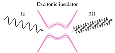
Figure 1: Schematic picture of THG in the excitonic insulator.

The rest of this paper is organized as follows. In Sec. II we introduce the model and time-dependent mean-field theory for the EI. Then, in Sec. III, we estimate the order parameter activated in the nonlinear regime and derive the THG susceptibility taking into account the vertex corrections. We show the calculated THG susceptibility in Sec. IV. Discussions and summary are given in Sec. V.

II Model

II.1 Two-band model

As a minimal theoretical model of the EI, we consider the spinless two-band correlated model (or extended Falicov-Kimball model) Ihle et al. (2008); Seki et al. (2011); Zenker et al. (2012); Kaneko et al. (2013); Ejima et al. (2014); Seki et al. (2014); Hamada et al. (2017); Kadosawa et al. (2020). The Hamiltonian takes the form

$$\hat{H}=\hat{H}_{0}+\hat{H}_{\rm int},$$ (1)

with

$$\hat{H}_{0}=-\sum_{\langle i,j\rangle}\sum_{\alpha}\left(t_{\alpha}\hat{c}_{i,\alpha}^{\dagger}\hat{c}_{j,\alpha}+{\rm H.c.}\right)+\sum_{j,\alpha}\Delta_{\alpha}\hat{c}_{j,\alpha}^{\dagger}\hat{c}_{j,\alpha},$$ (2)

$$\hat{H}_{\rm int}=U\sum_{j}\hat{c}_{j,0}^{\dagger}\hat{c}_{j,0}\hat{c}_{j,1}^{\dagger}\hat{c}_{j,1},$$ (3)

where $\hat{c}_{j,\alpha}$ ($\hat{c}_{j,\alpha}^{{\dagger}}$) is the annihilation (creation) operator of an electron at site $j$ on orbital $\alpha$ ($=0,1$), and $\langle i,j\rangle$ indicates a pair of nearest-neighbor sites. $t_{\alpha}$, $\Delta_{\alpha}$, and $U$ are the hopping integral, energy level of the orbital $\alpha$, and interorbital repulsive interaction, respectively. Here we focus on the half-filled case $n_{0}+n_{1}=\langle\hat{c}_{j,0}^{\dagger}\hat{c}_{j,0}\rangle+\langle\hat{c}_{j,1}^{\dagger}\hat{c}_{j,1}\rangle=1$ and consider the model defined on the two-dimensional (2D) square lattice ($d=2$). The free electron part in the momentum ($\bm{k}$) space is given by

$$\hat{H}_{0}=\sum_{\bm{k},\alpha}\varepsilon_{\alpha}(\bm{k})\hat{c}_{\bm{k},\alpha}^{\dagger}\hat{c}_{\bm{k},\alpha},$$ (4)

$$\varepsilon_{\alpha}(\bm{k})\equiv-2t_{\alpha}\left[\cos{\left(k_{x}a\right)}+\cos{\left(k_{y}a\right)}\right]+\Delta_{\alpha},$$ (5)

where we use the Fourier transformation $\hat{c}_{j,\alpha}=\frac{1}{\sqrt{N}}\sum_{\bm{k}}e^{i\bm{k}\cdot\bm{R}_{j}}\hat{c}_{\bm{k},\alpha}$ ($N$ is the number of lattice site), and $a$ is the lattice constant. We take the particle-hole symmetric band structure with $t_{0}=-t_{1}$ (direct-gap type) and assume $\Delta_{0}+\Delta_{1}=-U$ in order to set the Fermi energy to zero.

The external field $\bm{A}(t)$ is introduced by the Peierls substitution Tanabe et al. (2018); Fujiuchi et al. (2019), and we use the time-dependent Hamiltonian $\hat{H}(t)=\hat{H}_{0}(t)+\hat{H}_{\rm int}$, with

$$\hat{H}_{0}(t)=\sum_{\bm{k},\alpha}\varepsilon_{\alpha}\left(\bm{k}+\hbar^{-1}e\bm{A}(t)\right)\hat{c}_{\bm{k},\alpha}^{\dagger}\hat{c}_{\bm{k},\alpha},$$ (6)

where $e$ ($>0$) is the elementary charge and $\hbar$ is the Plank constant. In this paper we use the monochromatic continuous-wave $\bm{A}(t)=\bm{A}(\Omega)e^{-i\Omega t}+{\rm c.c.}$ unless otherwise noted. We assume that the interorbital dipole coupling $\bm{d}$ Murakami et al. (2017); Tanaka et al. (2018); Golež et al. (2020); Murakami et al. (2020) is zero for simplicity because it depends on the parities of the two orbitals.

II.2 Mean-field theory

In this paper we employ the time-dependent mean-field (tdMF) theory Murakami et al. (2017, 2020); Golež et al. (2020). We define the mean values of the diagonal and off-diagonal densities as

$$n_{\alpha}(t)=\left\langle\hat{c}_{j,\alpha}^{\dagger}(t)\hat{c}_{j,\alpha}(t)\right\rangle,\;\;\;\phi(t)=\left\langle\hat{c}_{j,0}^{\dagger}(t)\hat{c}_{j,1}(t)\right\rangle,$$ (7)

respectively, where the off-diagonal component $\phi(t)$ corresponds to the order parameter of the EI in our two-band model. Then, the MF Hamiltonian is given by

$$\hat{H}(t)\longrightarrow\hat{H}_{\mathrm{MF}}(t)=\sum_{\bm{k}}\sum_{\alpha,\alpha^{\prime}}h_{\alpha\alpha^{\prime}}^{A}(\bm{k},t)\hat{c}_{\bm{k},\alpha}^{\dagger}\hat{c}_{\bm{k},\alpha^{\prime}},$$ (8)

with

$$h^{A}(\bm{k},t)=h\left(\bm{k}+\hbar^{-1}e\bm{A}(t),\,t\right),$$ (9)

$$h(\bm{k},t)=\left[\begin{array}[]{cc}\varepsilon_{0}(\bm{k})+Un_{1}(t)&-U\phi^{*}(t)\\ -U\phi(t)&\varepsilon_{1}(\bm{k})+Un_{0}(t)\\ \end{array}\right],$$ (12)

where $h^{A}(\bm{k},t)$ is the matrix on the basis $\hat{\Psi}^{\dagger}_{\bm{k}}=[\hat{c}_{\bm{k},0}^{\dagger}\,\hat{c}_{\bm{k},1}^{\dagger}]$.

In the pseudospin representation, the Hamiltonian $h^{A}(\bm{k},t)$ is described by

$$h^{A}(\bm{k},t)=\frac{1}{2}\bm{B}(\bm{k},t)\cdot\bm{\sigma}+\frac{1}{2}B_{0}(\bm{k},t)\sigma_{0},$$ (13)

where $\sigma_{0}$ and $\sigma_{a}$ ($a=x,y,z$) are the identity and Pauli matrices, respectively,

$$B_{x}(\bm{k},t)= -2U\,{\mathrm{Re}}\,\phi(t),$$ (14)

$$B_{y}(\bm{k},t)= -2U\,{\mathrm{Im}}\,\phi(t),$$ (15)

$$B_{z}(\bm{k},t)= \;\varepsilon_{0}(\bm{k}+\hbar^{-1}e\bm{A}(t))-\varepsilon_{1}(\bm{k}+\hbar^{-1}e\bm{A}(t))$$

$$-U\left(n_{0}(t)-n_{1}(t)\right),$$ (16)

and $B_{0}(\bm{k},t)=0$ since we assume $t_{0}=-t_{1}$ and $\Delta_{0}+\Delta_{1}=-U$. Note that $B_{0}(\bm{k},t)=\varepsilon_{0}(\bm{k}+\hbar^{-1}e\bm{A}(t))+\varepsilon_{1}(\bm{k}+\hbar^{-1}e\bm{A}(t))+U$ when $t_{0}\neq-t_{1}$ and $\Delta_{0}+\Delta_{1}\neq-U$ at half-filling. In the pseudospin representation, the MF parameter is given by

$$\phi_{a}(t)=\frac{1}{2N}\sum_{\bm{k}}\left\langle\hat{\Psi}_{\bm{k}}^{\dagger}(t)\sigma_{a}\hat{\Psi}_{\bm{k}}(t)\right\rangle,$$ (17)

which composes the vector

$$\bm{\phi}(t)=\left[\begin{array}[]{c}\phi_{x}(t)\\ \phi_{y}(t)\\ \phi_{z}(t)\end{array}\right]=\left[\begin{array}[]{c}\mathrm{Re}\,\phi(t)\\ \mathrm{Im}\,\phi(t)\\ \left[n_{0}(t)-n_{1}(t)\right]/2\end{array}\right].$$ (24)

Then, the vector $\bm{B}(\bm{k},t)$ is given by

$$\bm{B}(\bm{k},t)=-2U\bm{\phi}(t)+2\xi(\bm{k}+\hbar^{-1}e\bm{A}(t))\bm{e}_{z},$$ (25)

where we define

$$\xi(\bm{k})\equiv\frac{\varepsilon_{0}(\bm{k})-\varepsilon_{1}(\bm{k})}{2}.$$ (26)

In the tdMF theory, the time-dependent current is determined by

$$J_{\mu}(t)=-e\sum_{\bm{k}}v_{\mu}\left(\bm{k}+\hbar^{-1}e\bm{A}(t)\right)\left\langle\hat{\Psi}^{\dagger}_{\bm{k}}(t)\sigma_{z}\hat{\Psi}_{\bm{k}}(t)\right\rangle,$$ (27)

where

$$v_{\mu}(\bm{k})\equiv\frac{1}{\hbar}\frac{\partial\xi({\bm{k}})}{\partial k_{\mu}}.$$ (28)

Note that, when $t_{0}\neq-t_{1}$, we need to include the $\sigma_{0}$ component in the current. When we perform the real-time simulations, we solve the equation of motion $\partial_{t}\bm{S}(\bm{k},t)=\hbar^{-1}\bm{B}(\bm{k},t)\times\bm{S}(\bm{k},t)$ for $S_{a}(\bm{k},t)\equiv\langle\hat{\Psi}_{\bm{k}}^{\dagger}(t)\sigma_{a}\hat{\Psi}_{\bm{k}}(t)\rangle/2$ with updating the MF parameter $\phi_{a}(t)$ simultaneously. In this paper we expand the nonequilibrium quantities and Green’s function with respect to the external field $\bm{A}(t)$ and estimate the photocurrent for THG.

In equilibrium [$B_{a}(\bm{k})=B_{a}(\bm{k},t=-\infty)$] we have the eigenenergy

$$E_{\pm}(\bm{k})=\hbar\omega_{\pm}(\bm{k})=\pm\frac{1}{2}\left|\bm{B}(\bm{k})\right|+\frac{1}{2}B_{0}(\bm{k}),$$ (29)

and the MF parameter is determined by

$$\phi_{a}=\frac{1}{N}\sum_{\bm{k}}\frac{B_{a}(\bm{k})}{2\left|\bm{B}(\bm{k})\right|}\left[f(E_{+}(\bm{k}))-f(E_{-}(\bm{k}))\right],$$ (30)

where $f(E)$ is the Fermi distribution function. We solve this equation self-consistently and determine the MF parameters in equilibrium. The bare lesser ($<$) and retarded/advanced ($R/A$) Green’s functions are given by

$$G^{0,<}(\bm{k},t)=i\sum_{\nu=\pm}f(E_{\nu}(\bm{k}))b_{\nu}(\bm{k})e^{-i\omega_{\nu}(\bm{k})t},$$ (31)

$$G^{0,R/A}(\bm{k},t)=\mp i\theta(\pm t)\sum_{\nu=\pm}b_{\nu}(\bm{k})e^{-i\omega_{\nu}(\bm{k})t},$$ (32)

respectively, where

$$b_{\nu}(\bm{k})=\frac{1}{2}\left[\sigma_{0}+\nu\frac{\bm{B}(\bm{k})}{\left|\bm{B}(\bm{k})\right|}\cdot\bm{\sigma}\right].$$ (33)

In the following we also use the Fourier transformed Green’s function $G^{0}(\bm{k},\omega)=\int dtG^{0}(\bm{k},t)e^{i\omega t}$.

III Nonlinear Responses

III.1 Perturbative expansion

Using the nonequilibrium Green’s function $G(\bm{k},t,t^{\prime})$ under the applied external field $\bm{A}(t)$ (see Appendix A), the MF parameter and current are given by

$$\phi_{a}(t)=-i\frac{1}{2N}\sum_{\bm{k}}{\mathrm{tr}}\left[\sigma_{a}G^{<}(\bm{k},t,t)\right],$$ (34)

$$J_{\mu}(t)=ie\sum_{\bm{k}}v_{\mu}\left(\bm{k}+\hbar^{-1}e\bm{A}(t)\right)\mathrm{tr}\left[\sigma_{z}G^{<}(\bm{k},t,t)\right],$$ (35)

respectively. In this section we expand the Green’s function (and velocity) with respect to the external field $\bm{A}(t)$ and derive the order parameter and current induced in the nonlinear regime.

With respect to $\bm{A}(t)$, we expand a quantity $X$ as

$$X(\bm{A}) =\sum_{n=0}^{\infty}X^{(n)}(\bm{A})=\sum_{n=0}^{\infty}\frac{1}{n!}\delta^{n}X(\bm{A}),$$ (36)

where $X^{(n)}(\bm{A})=\delta^{n}X(\bm{A})/n!=\mathcal{O}(A^{n})$. In this notation, the $n$th order variation of the Hamiltonian $h^{A}(\bm{k},t)$ is given by

$$\delta^{n}h^{A}(\bm{k},t)=-U\delta^{n}\bm{\phi}(t)\cdot\bm{\sigma}$$ (37)

$$+\left(\frac{e}{\hbar}\right)^{n}\sum_{\mu_{1},\cdots,\mu_{n}}\xi_{\mu_{1}\mu_{2}\cdots\mu_{n}}(\bm{k})A_{\mu_{1}}(t)A_{\mu_{2}}(t)\cdots A_{\mu_{n}}(t)\,\sigma_{z},$$

where

$$\xi_{\mu_{1}\cdots\mu_{n}}(\bm{k})\equiv\frac{\partial^{n}\xi(\bm{k})}{\partial k_{\mu_{1}}\partial k_{\mu_{2}}\cdots\partial k_{\mu_{n}}}.$$ (38)

We expand the Green’s function $G$ with respect to the deviation from equilibrium $\delta^{n}\mathcal{H}$ given by $\delta^{n}h^{A}(\bm{k},t)$. The details of the nonequilibrium Green’s function and its expansion are summarized in Appendix A. Expanding the Green’s function up to the third order, we have

$$\delta G =G^{0}*\delta\mathcal{H}*G^{0},$$ (39)

$$\delta^{2}G =2G^{0}*\delta\mathcal{H}*G^{0}*\delta\mathcal{H}*G^{0}$$

$$+G^{0}*\delta^{2}\mathcal{H}*G^{0},$$ (40)

$$\delta^{3}G =6G^{0}*\delta\mathcal{H}*G^{0}*\delta\mathcal{H}*G^{0}*\delta\mathcal{H}*G^{0}$$

$$+3G^{0}*\delta\mathcal{H}*G^{0}*\delta^{2}\mathcal{H}*G^{0}$$

$$+3G^{0}*\delta^{2}\mathcal{H}*G^{0}*\delta\mathcal{H}*G^{0}$$

$$+G^{0}*\delta^{3}\mathcal{H}*G^{0},$$ (41)

where $X*Y$ indicates the product including the time-integration $\int dt_{1}X^{\zeta\zeta_{1}}(t,t_{1})Y^{\zeta_{1}\zeta^{\prime}}(t_{1},t^{\prime})$ (see details in Appendix A) Aoki et al. (2014).

In the following, we estimate the MF parameter $\delta^{2}\phi_{a}$ at second order and then derive the nonlinear current $\delta^{3}J_{\mu}$ for THG involving the collective dynamics of the order parameter (i.e., vertex correction).

III.2 Order parameter

First, we derive the order parameter away from equilibrium by expanding the Green’s function. Because of the symmetry under inversion, e.g., $\xi_{\mu}(-\bm{k})=-\xi_{\mu}(\bm{k})$, the MF parameters at odd order [$\delta\bm{\phi}(t)$, $\delta^{3}\bm{\phi}(t)$, $\cdots$] vanish (see Appendix B). Hence, the lowest order of the activated order parameter is of the second order;

$$\delta^{2}\phi_{a}(t)=-i\frac{1}{2N}\sum_{\bm{k}}{\mathrm{tr}}\left[\sigma_{a}\delta^{2}G^{<}(\bm{k},t,t)\right].$$ (42)

Under the monochromatic field $\bm{A}(t)=\bm{A}(\Omega)e^{-i\Omega t}+\bm{A}(-\Omega)e^{i\Omega t}$, the MF parameter at second order is characterized by $\delta^{2}\phi_{a}(t)=\delta^{2}\phi_{a}(2\Omega)e^{-2i\Omega t}+\delta^{2}\phi_{a}(-2\Omega)e^{2i\Omega t}+\delta^{2}\phi_{a}(0)$. While $\delta^{2}\phi_{a}(0)$ [$\propto A(\Omega)A(-\Omega)$] can be nonzero, it does not contribute to THG given by $\delta^{3}J(3\Omega)$ [$\propto A(\Omega)^{3}$]. Here, we consider $\delta^{2}\phi_{a}(2\Omega)$ [$\propto A(\Omega)^{2}$] because THG originated from the dynamical order parameter (vertex correction) is described by $\delta^{3}J^{\rm vc}(3\Omega)\propto\delta^{2}\phi_{a}(2\Omega)A(\Omega)$. Combining Eqs. (40) and (42), $\delta^{2}\phi_{a}(2\Omega)$ is given by

$$\delta^{2}\phi_{a}(2\Omega)= -i\frac{1}{2N}\sum_{\bm{k}}\frac{2}{\hbar^{2}}\int\frac{d\omega}{2\pi}{\mathrm{tr}}\left[\sigma_{a}G^{0}(\bm{k},\omega+2\Omega)\delta h^{A}(\bm{k},\Omega)G^{0}(\bm{k},\omega+\Omega)\delta h^{A}(\bm{k},\Omega)G^{0}(\bm{k},\omega)\right]^{<}$$

$$-i\frac{1}{2N}\sum_{\bm{k}}\frac{1}{\hbar}\int\frac{d\omega}{2\pi}{\mathrm{tr}}\left[\sigma_{a}G^{0}(\bm{k},\omega+2\Omega)\delta^{2}h^{A}(\bm{k},2\Omega)G^{0}(\bm{k},\omega)\right]^{<},$$ (43)

where $[\cdots]^{<}$ indicates the lesser component following the Langreth’s rule, e.g., $[XY]^{<}=X^{R}Y^{<}+X^{<}Y^{A}$ (see details in Appendix A). While we can integrate the Green’s functions over $\omega$ as summarized in Appendix C, we retain the $\omega$ integral with the Green’s functions for the compact notation. Since $\delta\bm{\phi}(t)=0$ (see Appendix B), we have

$$\delta h^{A}(\bm{k},\Omega)=\frac{e}{\hbar}\sum_{\mu_{1}}\xi_{\mu_{1}}(\bm{k})A_{\mu_{1}}(\Omega)\,\sigma_{z},$$ (44)

but $\delta^{2}\bm{\phi}(2\Omega)$ can be nonzero and

$$\delta^{2}h^{A}(\bm{k},2\Omega)=-U\delta^{2}\bm{\phi}(2\Omega)\cdot\bm{\sigma}+\left(\frac{e}{\hbar}\right)^{2}\sum_{\mu_{1},\mu_{2}}\xi_{\mu_{1}\mu_{2}}(\bm{k})A_{\mu_{1}}(\Omega)A_{\mu_{2}}(\Omega)\,\sigma_{z}.$$ (45)

Equation (43) corresponds to the self-consistent equation of $\delta^{2}\bm{\phi}(2\Omega)$ because $\delta^{2}h^{A}(\bm{k},2\Omega)$ in the right-hand side of Eq. (43) includes $\delta^{2}\bm{\phi}(2\Omega)$.

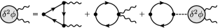
Figure 2: The diagrammatic representation of Eq.(49). The solid (with arrow), wavy, and dashed lines indicate the bare Green’s function $G^{0}$, external field $\bm{A}$, and interaction $U$, respectively.

Introducing the bare susceptibilities for coupling between the order parameter $\phi$ and the external field $A_{\mu}(\Omega)$,

$$\bm{\chi}^{0;\phi\xi\xi}_{\mu_{1}\mu_{2}}(2\Omega;\Omega,\Omega) =-i\frac{1}{\hbar^{2}}\frac{1}{N}\sum_{\bm{k}}\int\frac{d\omega}{2\pi}{\mathrm{tr}}\left[\bm{\sigma}G^{0}(\bm{k},\omega+2\Omega)\sigma_{z}G^{0}(\bm{k},\omega+\Omega)\sigma_{z}G^{0}(\bm{k},\omega)\right]^{<}\xi_{\mu_{1}}(\bm{k})\xi_{\mu_{2}}(\bm{k}),$$ (46)

$$\bm{\chi}^{0;\phi\xi}_{\mu_{1}\mu_{2}}(2\Omega;2\Omega) =-i\frac{1}{2\hbar}\frac{1}{N}\sum_{\bm{k}}\int\frac{d\omega}{2\pi}{\mathrm{tr}}\left[\bm{\sigma}G^{0}(\bm{k},\omega+2\Omega)\sigma_{z}G^{0}(\bm{k},\omega)\right]^{<}\xi_{\mu_{1}\mu_{2}}(\bm{k}),$$ (47)

and the bare $\phi$-$\phi$ susceptibility ($3\times 3$ matrix)

$$\left[\tilde{\chi}^{0;\phi\phi}(2\Omega)\right]_{ab}=-i\frac{1}{2\hbar}\frac{1}{N}\sum_{\bm{k}}\int\frac{d\omega}{2\pi}{\mathrm{tr}}\left[\sigma_{a}G^{0}(\bm{k},\omega+2\Omega)\sigma_{b}G^{0}(\bm{k},\omega)\right]^{<},$$ (48)

the self-consistent Eq. (43) becomes

$$\delta^{2}\!\bm{\phi}(2\Omega)=\left(\frac{e}{\hbar}\right)^{2}\!\sum_{\mu_{1},\mu_{2}}\!\bm{\chi}^{0;\phi\xi\xi}_{\mu_{1}\mu_{2}}(2\Omega;\Omega,\Omega)A_{\mu_{1}}(\Omega)A_{\mu_{2}}(\Omega)+\left(\frac{e}{\hbar}\right)^{2}\!\sum_{\mu_{1},\mu_{2}}\!\bm{\chi}^{0;\phi\xi}_{\mu_{1}\mu_{2}}(2\Omega;2\Omega)A_{\mu_{1}}(\Omega)A_{\mu_{2}}(\Omega)-U\tilde{\chi}^{0;\phi\phi}(2\Omega)\delta^{2}\!\bm{\phi}(2\Omega).$$ (49)

This equation may be described by the diagrams in Fig. 2 Tsuji and Aoki (2015). Then we obtain the solution

$$\delta^{2}\bm{\phi}(2\Omega)=\left(\frac{e}{\hbar}\right)^{2}\sum_{\mu_{1},\mu_{2}}\frac{\bm{\chi}^{0;\phi\xi\xi}_{\mu_{1}\mu_{2}}(2\Omega;\Omega,\Omega)}{1+U\tilde{\chi}^{0;\phi\phi}(2\Omega)}A_{\mu_{1}}(\Omega)A_{\mu_{2}}(\Omega)+\left(\frac{e}{\hbar}\right)^{2}\sum_{\mu_{1},\mu_{2}}\frac{\bm{\chi}^{0;\phi\xi}_{\mu_{1}\mu_{2}}(2\Omega;2\Omega)}{1+U\tilde{\chi}^{0;\phi\phi}(2\Omega)}A_{\mu_{1}}(\Omega)A_{\mu_{2}}(\Omega),$$ (50)

indicating that the order parameter is activated at second order of $\bm{A}$ when the corrected susceptibility is nonzero. For later convenience we express the above relation as

$$\delta^{2}\phi_{a}(2\Omega)=\left(\frac{e}{\hbar}\right)^{2}\sum_{\mu_{1},\mu_{2}}\Gamma_{\mu_{1}\mu_{2}}^{a}(2\Omega;\Omega,\Omega)A_{\mu_{1}}(\Omega)A_{\mu_{2}}(\Omega),$$ (51)

with

$$\bm{\Gamma}_{\mu_{1}\mu_{2}}(2\Omega;\Omega,\Omega) =\frac{\bm{\chi}^{0;\phi\xi\xi}_{\mu_{1}\mu_{2}}(2\Omega;\Omega,\Omega)}{1+U\tilde{\chi}^{0;\phi\phi}(2\Omega)}+\frac{\bm{\chi}^{0;\phi\xi}_{\mu_{1}\mu_{2}}(2\Omega;2\Omega)}{1+U\tilde{\chi}^{0;\phi\phi}(2\Omega)}.$$ (52)

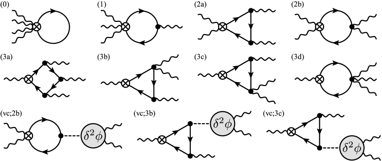
Figure 3: The diagrams for the third-order photocurrent. The solid (with arrow), wavy, and dashed lines indicate the bare Green’s function $G^{0}$, external field $\bm{A}$, and interaction $U$, respectively. The cross indicates the one-photon output.

III.3 Current

Next, we derive the nonlinear current involving the dynamics of the order parameter. Expanding $J_{\mu}(t)$ in Eq. (35), the current at $n$th order is given by

$$\delta^{n}\!J_{\mu}(t)\!=\!ie\!\sum_{\bm{k}}\sum_{m=0}^{n}\!\binom{n}{m}\delta^{n-m}v^{A}_{\mu}(\bm{k},t){\mathrm{tr}}\left[\sigma_{z}\delta^{m}G^{<}(\bm{k},t,t)\right],$$ (53)

where $\binom{n}{m}$ is binomial coefficient and

$$\delta^{n}v^{A}_{\mu}(\bm{k},t)=\frac{e^{n}}{\hbar^{n+1}}\!\sum_{\mu_{1},\cdots,\mu_{n}}\!\xi_{\mu\mu_{1}\cdots\mu_{n}}(\bm{k})A_{\mu_{1}}(t)\cdots A_{\mu_{n}}(t).$$ (54)

The linear response $\delta J_{\mu}(t)$ can be nonzero in the EI state. However, because $\delta\bm{\phi}(t)=0$, the linear optical response does not reflect the dynamical effect of the order parameter. The second-order response $\delta^{2}J_{\mu}(t)$ vanishes in the inversion symmetric system because the current has odd parity under inversion. Hence, in order to see the dynamics of the excitonic order parameter, we need to evaluate the optical response at third order.

Combining Eqs. (39)-(41), (53), and (54), we derive the third-order current $\delta^{3}J_{\mu}$, which is comprised of the contributions diagrammatically described in Fig. 3 Parker et al. (2019). Since the order parameter $\delta^{2}\bm{\phi}(t)$ is included only in $\delta^{2}h^{A}(\bm{k},t)$, the contributions 2b, 3b, and 3c are affected by the dynamical order parameter, which leads to the vertex correction terms (see Fig. 3). Here, as an example, we derive the contribution from 3b but all the THG susceptibilities are summarized in Appendix D. $v_{\mu}(\bm{k})$ and $G^{0}\!*\!\delta\mathcal{H}\!*\!G^{0}\!*\!\delta^{2}\mathcal{H}\!*\!G^{0}$ in $\delta^{3}G$ gives $\delta^{3}J_{\mu}(3\Omega)$ of 3b,

$$\delta^{3}J_{\mu}(3\Omega)_{3b} =3i\left(\frac{e}{\hbar}\right)\sum_{\bm{k}}\xi_{\mu}(\bm{k})\frac{1}{\hbar^{2}}\int\frac{d\omega}{2\pi}{\mathrm{tr}}\left[\sigma_{z}G^{0}(\bm{k},\omega+3\Omega)\delta h^{A}(\bm{k},\Omega)G^{0}(\bm{k},\omega+2\Omega)\delta^{2}h^{A}(\bm{k},2\Omega)G^{0}(\bm{k},\omega)\right]^{<}.$$ (55)

Dividing as $\delta^{3}J_{\mu}(3\Omega)=\delta^{3}J^{0}_{\mu}(3\Omega)+\delta^{3}J^{\rm vc}_{\mu}(3\Omega)$, the bare (0) and vertex correction (vc) terms are given by

$$\delta^{3}J^{0}_{\mu}(3\Omega)_{3b} =3i\left(\frac{e}{\hbar}\right)^{4}\sum_{\mu_{1},\mu_{2},\mu_{3}}\sum_{\bm{k}}\frac{1}{\hbar^{2}}\int\frac{d\omega}{2\pi}{\mathrm{tr}}\left[\sigma_{z}G^{0}(\bm{k},\omega+3\Omega)\sigma_{z}G^{0}(\bm{k},\omega+2\Omega)\sigma_{z}G^{0}(\bm{k},\omega)\right]^{<}$$

$$\hskip 170.0pt\times\xi_{\mu}(\bm{k})\xi_{\mu_{1}}(\bm{k})\xi_{\mu_{2}\mu_{3}}(\bm{k})A_{\mu_{1}}(\Omega)A_{\mu_{2}}(\Omega)A_{\mu_{3}}(\Omega),$$ (56)

$$\delta^{3}J^{\rm vc}_{\mu}(3\Omega)_{3b} =-3iU\left(\frac{e}{\hbar}\right)^{4}\sum_{\mu_{1},\mu_{2},\mu_{3}}\sum_{a}\sum_{\bm{k}}\frac{1}{\hbar^{2}}\int\frac{d\omega}{2\pi}{\mathrm{tr}}\left[\sigma_{z}G^{0}(\bm{k},\omega+3\Omega)\sigma_{z}G^{0}(\bm{k},\omega+2\Omega)\sigma_{a}G^{0}(\bm{k},\omega)\right]^{<}$$

$$\hskip 170.0pt\times\xi_{\mu}(\bm{k})\xi_{\mu_{1}}(\bm{k})\Gamma_{\mu_{2}\mu_{3}}^{a}(2\Omega;\Omega,\Omega)A_{\mu_{1}}(\Omega)A_{\mu_{2}}(\Omega)A_{\mu_{3}}(\Omega),$$ (57)

respectively, where the vertex correction term $\delta^{3}J^{\rm vc}_{\mu}(3\Omega)$ arises from the order parameter $\delta^{2}\phi(2\Omega)$ in Eq. (51). The THG susceptibility may be defined as

$$J^{(3)}_{\mu}(3\Omega)=\delta^{3}J_{\mu}(3\Omega)/3!=L^{d}\sum_{\mu_{1},\mu_{2},\mu_{3}}\chi^{(3)}_{\mu;\mu_{1}\mu_{2}\mu_{3}}(3\Omega;\Omega)A_{\mu_{1}}(\Omega)A_{\mu_{2}}(\Omega)A_{\mu_{3}}(\Omega),$$ (58)

where $\chi^{(3)}_{\mu;\mu_{1}\mu_{2}\mu_{3}}(3\Omega;\Omega)=\chi^{(3)}_{\mu;\mu_{1}\mu_{2}\mu_{3}}(3\Omega;\Omega,\Omega,\Omega)$ and $L^{d}$ is the volume. Dividing $\chi^{(3)}_{\mu;\mu_{1}\mu_{2}\mu_{3}}(3\Omega;\Omega)$ into $\chi^{0;(3)}_{\mu;\mu_{1}\mu_{2}\mu_{3}}(3\Omega;\Omega)$ and $\chi^{{\rm vc};(3)}_{\mu;\mu_{1}\mu_{2}\mu_{3}}(3\Omega;\Omega)$, the bare and vertex correction terms of 3b are given by

$$\chi^{0;(3,3b)}_{\mu;\mu_{1}\mu_{2}\mu_{3}}(3\Omega;\Omega) =\frac{1}{2}i\left(\frac{e}{\hbar}\right)^{4}\frac{1}{\hbar^{2}}\int\!\frac{d\bm{k}}{(2\pi)^{d}}\!\int\!\frac{d\omega}{2\pi}\mathrm{tr}\left[\sigma_{z}G^{0}(\bm{k},\omega\!+\!3\Omega)\sigma_{z}G^{0}(\bm{k},\omega\!+\!2\Omega)\sigma_{z}G^{0}(\bm{k},\omega)\right]^{<}$$

$$\hskip 235.0pt\times\xi_{\mu}(\bm{k})\xi_{\mu_{1}}(\bm{k})\xi_{\mu_{2}\mu_{3}}(\bm{k}),$$ (59)

$$\chi^{{\rm vc};(3,3b)}_{\mu;\mu_{1}\mu_{2}\mu_{3}}(3\Omega;\Omega) =-\frac{U}{2}i\left(\frac{e}{\hbar}\right)^{4}\frac{1}{\hbar^{2}}\int\!\frac{d\bm{k}}{(2\pi)^{d}}\!\int\!\frac{d\omega}{2\pi}\sum_{a}{\mathrm{tr}}\left[\sigma_{z}G^{0}(\bm{k},\omega\!+\!3\Omega)\sigma_{z}G^{0}(\bm{k},\omega\!+\!2\Omega)\sigma_{a}G^{0}(\bm{k},\omega)\right]^{<}$$

$$\hskip 235.0pt\times\xi_{\mu}(\bm{k})\xi_{\mu_{1}}(\bm{k})\Gamma_{\mu_{2}\mu_{3}}^{a}(2\Omega;\Omega,\Omega),$$ (60)

respectively. In the same way, we can derive the other THG susceptibilities and their formulas are summarized in Appendix D. Because of the vertex correction $\chi^{{\rm vc};(3)}_{\mu;\mu_{1}\mu_{2}\mu_{3}}(3\Omega;\Omega)$, the THG susceptibility can reflect the collective dynamics in the EI.

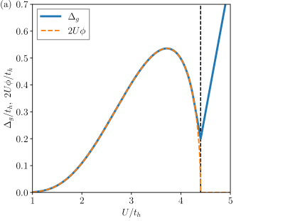
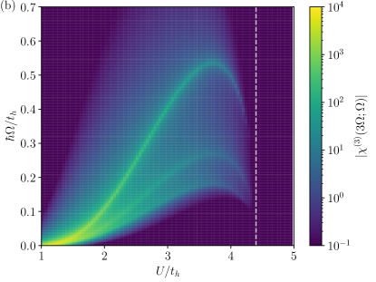
Figure 4: (a) $U$ dependence of the excitonic order parameter $U\phi$ and the band gap $\Delta_{g}$ in the ground state. The energy level difference is $D=\Delta_{0}-\Delta_{1}=3.8t_{h}$ and the vertical dashed line indicates the boundary of the EI phase ($U_{c}$). (b) THG susceptibility $|\chi^{(3)}_{x;xxx}(3\Omega;\Omega)|$ in the plane of $U$ and $\Omega$. $|\chi^{(3)}_{x;xxx}(3\Omega;\Omega)|$ is plotted in units of $(e/\hbar)^{4}a^{2}t_{h}$ and the damping factor $\eta=0.005t_{h}$ is used.

IV Third-harmonic generation

IV.1 THG susceptibility in the EI

First, we show the THG susceptibility $\chi_{\mu;\mu_{1}\mu_{2}\mu_{3}}^{(3)}(3\Omega;\Omega)$ at zero temperature. Here we assume that the order parameter $\phi$ is real in the ground state without loss of generality and the external field is polarized along the $x$ direction. The polarization direction of the incident light does not change the main features of the THG susceptibility in the EI and the polarization dependence is discussed in Appendix E. Here we set $t_{h}$ as a unit of the energy and plot the THG susceptibility $\chi_{x;xxx}^{(3)}(3\Omega;\Omega)$ in units of $(ea/\hbar)^{4}t_{h}/a^{d}$ on the 2D square lattice ($d=2$).

In order to see the change of the THG susceptibility from the BCS (small-$U$, semimetallic) regime to the BEC (large-$U$, semiconducting) regime, we plot the data by changing the Coulomb interaction $U$. Figure 4(a) shows the $U$ dependence of the band gap $\Delta_{g}$ and order parameter $\phi$ in the ground state. While $\Delta_{g}=2U\phi$ in the BCS regime, $\Delta_{g}>2U\phi$ in the BEC semiconducting regime Seki et al. (2011). The order parameter vanishes above the phase boundary $U>U_{c}$, where the band gap $\Delta_{g}$ is larger than the exciton binding energy $E_{B}$ Murakami et al. (2020). Figure 4(b) is one of our main results, where we plot the magnitude of the THG susceptibility $|\chi_{x;xxx}^{(3)}(3\Omega;\Omega)|$ as a function of $U$. $\chi_{x;xxx}^{(3)}(3\Omega;\Omega)$ exhibits three peaks in the EI phase and their positions correspond to $\hbar\Omega=\Delta_{g}/3$, $\Delta_{g}/2$, and $\Delta_{g}$ from the bottom. The THG response is strong in the BCS regime but it becomes less prominent with approaching the phase boundary $U_{c}$.

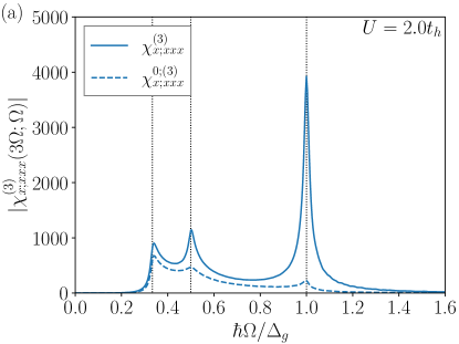
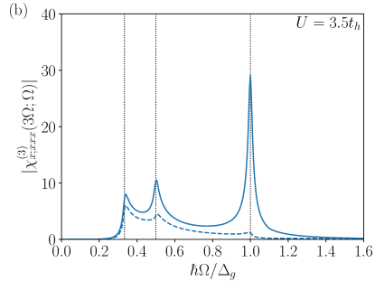
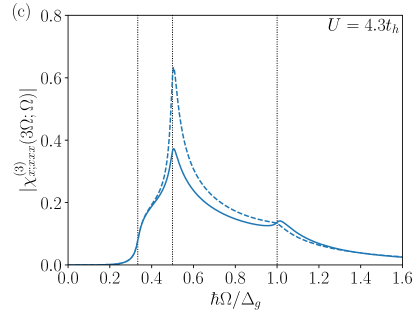
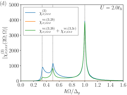
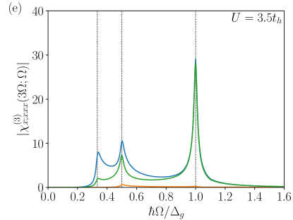
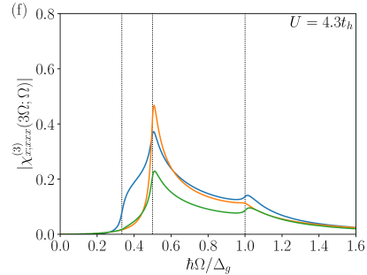
Figure 5: THG susceptibility $|\chi^{(3)}_{x;xxx}(3\Omega;\Omega)|$ at (a) and (d) $U=2t_{h}$ (BCS regime), (b) and (e) $U=3.5t_{h}$ (intermediate regime), and (c) and (f) $U=4.3t_{h}$ (BEC regime), where the horizontal axis is scaled by the band gap $\Delta_{g}$. For comparison, the bare susceptibility $\chi^{0;(3)}_{x;xxx}(3\Omega;\Omega)$ is plotted in the upper panels [(a)-(c)] and the vertex corrections $\chi^{{\rm vc};(3,2b)}_{x;xxx}(3\Omega;\Omega)$ and $\chi^{{\rm vc};(3,3b)}_{x;xxx}(3\Omega;\Omega)+\chi^{{\rm vc};(3,3c)}_{x;xxx}(3\Omega;\Omega)$ (see Fig. 3) are plotted in the lower panels [(d)-(f)]. The vertical dotted lines indicates $\hbar\Omega=\Delta_{g}/3$, $\Delta_{g}/2$, and $\Delta_{g}$. Here $\eta=0.01\Delta_{g}$ is used while the other parameters are the same as in Fig. 4.

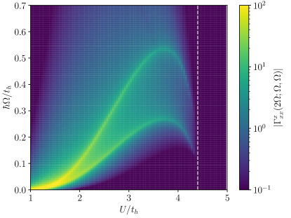
Figure 6: Second-order response function for the order parameter $|\Gamma^{x}_{xx}(2\Omega;\Omega,\Omega)|$ in the plane of $U$ and $\Omega$. The vertical dashed line indicates the boundary of the EI phase ($U_{c}$). Here $|\Gamma^{x}_{xx}(2\Omega;\Omega,\Omega)|$ is plotted in units of $a^{2}$ and the energy level difference $D=\Delta_{0}-\Delta_{1}=3.8t_{h}$ and the damping factor $\eta=0.005t_{h}$ are used.

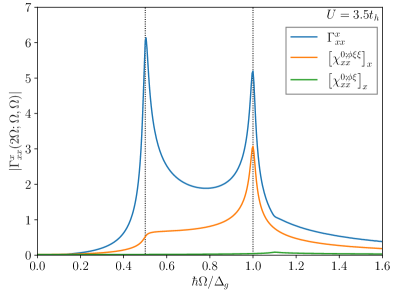
Figure 7: Second-order response function for the order parameter $|\Gamma^{x}_{xx}(2\Omega;\Omega,\Omega)|$ at $U=3.5t_{h}$, where the horizontal axis is scaled by the band gap $\Delta_{g}$. For comparison, the bare response functions $\left[\chi_{xx}^{0;\phi\xi\xi}(2\Omega;\Omega,\Omega)\right]_{x}$ and $\left[\chi_{xx}^{0;\phi\xi}(2\Omega;2\Omega)\right]_{x}$ are plotted. The vertical dotted lines indicates $\hbar\Omega=\Delta_{g}/2$, and $\Delta_{g}$. Here $\eta=0.01\Delta_{g}$ is used while the other parameters are the same as in Fig. 6.

Figure 5 shows the THG susceptibility as a function of $\hbar\Omega/\Delta_{g}$ in the BCS and BEC regimes. Here, in order to identify the contributions from the vertex correction, we plot the bare susceptibility $\chi^{0;(3)}_{x;xxx}(3\Omega;\Omega)$ in Figs. 5(a)-5(c) and the vertex corrections $\chi^{{\rm vc};(3,2b)}_{x;xxx}(3\Omega;\Omega)$ and $\chi^{{\rm vc};(3,3b)}_{x;xxx}(3\Omega;\Omega)+\chi^{{\rm vc};(3,3c)}_{x;xxx}(3\Omega;\Omega)$ in Figs. 5(d)-5(f). All components of the bare THG susceptibilities and vertex corrections are presented in Appendix D. As shown in Fig. 5, while the THG susceptibility at $\hbar\Omega=\Delta_{g}/3$ is mainly composed of the bare part $\chi^{0;(3)}_{x;xxx}(3\Omega;\Omega)$, the magnitude at $\hbar\Omega=\Delta_{g}/2$ and $\Delta_{g}$ are modified by the vertex part $\chi^{{\rm vc};(3)}_{x;xxx}(3\Omega;\Omega)$. This indicates that, while THG at $\hbar\Omega=\Delta_{g}/3$ is simply caused by bare three-photon excitation of the independent particle across the band gap $\Delta_{g}$, the order-parameter motions strongly contribute to THG at $\hbar\Omega=\Delta_{g}/2$ and $\Delta_{g}$.

In the BCS regime, the vertex correction enhances the THG susceptibility at both $\hbar\Omega=\Delta_{g}/2$ and $\Delta_{g}$. In particular, the peak at $\hbar\Omega=\Delta_{g}$ is outstanding. As shown in Figs. 5(d) and 5(e), while the vertex correction in 2b (see Fig. 3) is much smaller than the bare susceptibility, the vertex corrections in 3b and 3c (see Fig. 3) dominantly enhance THG at $\hbar\Omega=\Delta_{g}/2$ and bring the significant peak at $\hbar\Omega=\Delta_{g}$. Hence, we can observe the strong THG response due to the order-parameter motion, which is emergent in $\chi^{{\rm vc};(3,3b)}_{x;xxx}(3\Omega;\Omega)$ and $\chi^{{\rm vc};(3,3c)}_{x;xxx}(3\Omega;\Omega)$.

In the BEC semiconducting regime, on the other hand, the peaks at $\hbar\Omega=\Delta_{g}/2$ and $\Delta_{g}$ in the THG susceptibility become less prominent. As shown in Fig. 5(c), $|\chi^{(3)}_{x;xxx}(3\Omega;\Omega)|$ at $\hbar\Omega=\Delta_{g}/2$ is suppressed from the value of the bare susceptibility $|\chi^{0;(3)}_{x;xxx}(3\Omega;\Omega)|$. The vertex correction in 3b and 3c is much smaller than its value in the BCS regime and is comparable to the vertex correction in 2b [see Fig. 5(f)]. Since the vertex corrections are weak in the BEC regime, the resulting THG susceptibility does not show the collective excitonic nature strongly.

Since the collective order parameter dynamics is important for THG in the EI, we show $\Gamma^{a}_{\mu_{1}\mu_{2}}(2\Omega;\Omega,\Omega)$ in Figs. 6 and 7, which is the response function of the MF parameter at second order in $\bm{A}(\Omega)$ [see Eq. (51)]. Because we assume the order parameter $\phi$ is real in the ground state, the $a=x$ and $y$ components indicate the amplitude and phase oscillations of the order parameter, respectively. The $a=z$ component $\Gamma^{z}_{\mu_{1}\mu_{2}}(2\Omega;\Omega,\Omega)$ is zero when the hopping parameters satisfy $t_{0}+t_{1}=0$ at half-filling. While the $a=y$ (phase) component is nonzero, the $a=x$ (amplitude) component is dominant in particular in the BCS regime and here we present $\Gamma^{x}_{xx}(2\Omega;\Omega,\Omega)$. Figure 6 shows $\Gamma^{x}_{xx}(2\Omega;\Omega,\Omega)$ in the plane of $U$ and $\Omega$, where we find two peaks at $\hbar\Omega=\Delta_{g}/2$ and $\Delta_{g}$. The response of the amplitude oscillation is strong in the BCS regime but it becomes weaker with approaching the phase boundary $U_{c}$.

In order to identify the origin of the two-peak structure, we compare $\Gamma^{x}_{xx}(2\Omega;\Omega,\Omega)$ with the bare response functions $\left[\chi_{xx}^{0;\phi\xi\xi}(2\Omega;\Omega,\Omega)\right]_{x}$ and $\left[\chi_{xx}^{0;\phi\xi}(2\Omega;2\Omega)\right]_{x}$ in Eqs. (46) and (47), respectively. As shown in Fig. 7, while the contribution from $\left[\chi_{xx}^{0;\phi\xi}(2\Omega;2\Omega)\right]_{x}$ is minor, $\left[\chi_{xx}^{0;\phi\xi\xi}(2\Omega;\Omega,\Omega)\right]_{x}$ exhibits the sharp peak at $\hbar\Omega=\Delta_{g}$, which is enhanced by the many-body correction in $\Gamma^{x}_{xx}(2\Omega;\Omega,\Omega)$. The response at $\hbar\Omega=\Delta_{g}/2$ is not prominent in the bare function, but the many-body correction $\left[1+U\tilde{\chi}^{\phi\phi}\right]^{-1}$ in $\Gamma^{x}_{xx}(2\Omega;\Omega,\Omega)$ gives rise to the resonant peak at $\hbar\Omega=\Delta_{g}/2$. Therefore, the origins of the peaks at $\hbar\Omega=\Delta_{g}/2$ and $\Delta_{g}$ are different, where the response at $\hbar\Omega=\Delta_{g}/2$ is originated by the many-body correction in $\Gamma^{x}_{xx}(2\Omega;\Omega,\Omega)$ while the response at $\hbar\Omega=\Delta_{g}$ is mainly caused by the bare photon absorption described by the loop triangle diagram in Fig. 2. Using Eq. (93) for the the loop triangle diagram, we find that $\left[\chi_{xx}^{0;\phi\xi\xi}(2\Omega;\Omega,\Omega)\right]_{x}$ includes the contribution represented by $(2\hbar\Omega)^{-1}\sum_{\bm{k}}\lambda(\bm{k})/\left[\hbar\Omega-|\bm{B}(\bm{k})|\right]$, which arises when one of two photon absorptions is resonant. This contribution gives rise to the prominent peak at $\hbar\Omega=\Delta_{g}$ in Fig. 7.

Since $\Gamma^{a}_{\mu_{1}\mu_{2}}(2\Omega;\Omega,\Omega)$ gives the vertex corrections in the THG susceptibility, two peaks observed in $\Gamma^{x}_{xx}(2\Omega;\Omega,\Omega)$ bring the resonant enhancement of THG at $\hbar\Omega=\Delta_{g}/2$ and $\Delta_{g}$. In the BEC regime, the vertex correction is small as shown in Fig. 6 and the resulting THG susceptibility does not exhibit significant peaks in comparison with the BCS-type EI. This is because the order parameter in the BEC-type EI is deeply stabilized at the bottom of the energy and is hard to deviate from its equilibrium value at second order in $\bm{A}(\Omega)$.

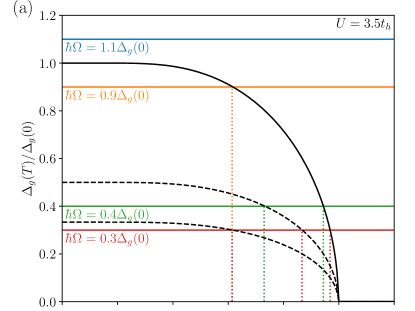
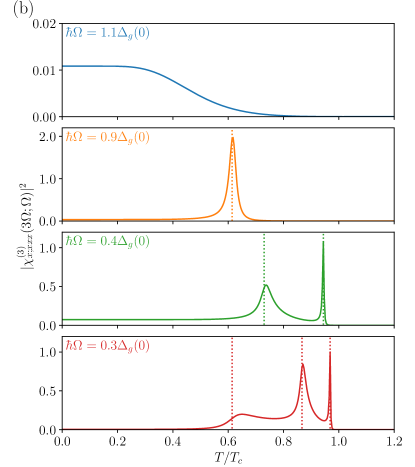
Figure 8: (a) Temperature dependence of the band gap $\Delta_{g}(T)$ at $U=3.5t_{h}$, where the dashed lines indicate $\Delta_{g}(T)/2$ and $\Delta_{g}(T)/3$. The vertical dotted line indicates the temperature at which the order parameter and $\hbar\Omega$ cross. (b) Temperature dependence of $|\chi^{(3)}_{x;xxx}(3\Omega;\Omega)|^{2}$. All intensities are normalized to the maximum value at $\hbar\Omega=0.3\Delta_{g}(T=0)$. The energy level difference $D=\Delta_{0}-\Delta_{1}=3.8t_{h}$ and the damping factor $\eta=0.01\Delta_{g}(0)$ are used.

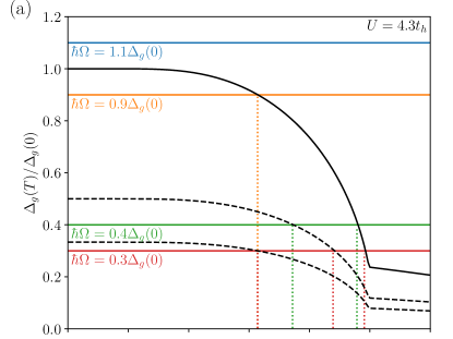
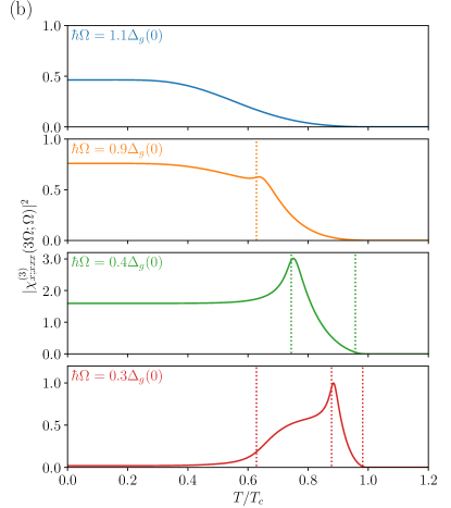
Figure 9: Same as Fig. 8 but at $U=4.3t_{h}$ (BEC regime).

IV.2 Temperature dependence of the THG intensity

In the discussions of the Higgs-mode resonance in superconductors, the temperature profile of the THG intensity is compared with experimental THG response Cea et al. (2016); Schwarz and Manske (2020); Matsunaga et al. (2014); Shimano and Tsuji (2020). Hence, we show the temperature dependence of the THG intensity for the EI fin . Here, we plot $|\chi^{(3)}_{x;xxx}(3\Omega;\Omega)|^{2}$ as the THG intensity $I_{\rm THG}$ since $I_{\rm THG}\propto|J^{(3)}_{\mu}(3\Omega)|^{2}$.

Figure 8 shows the results at $U=3.5t_{h}$, where the strong THG responses are anticipated at $\hbar\Omega=\Delta_{g}$, $\Delta_{g}/2$, and $\Delta_{g}/3$ as shown in Fig. 5(b). Actually, the temperature dependent THG intensity in Fig. 8(b) exhibits three peaks at the temperatures when $\hbar\Omega=0.3\Delta_{g}(T\!=\!0)$ crosses $\Delta_{g}(T)$, $\Delta_{g}(T)/2$, and $\Delta_{g}(T)/3$, respectively. Associated with the number of the crossing points [see Fig. 8(a)], the THG intensities at $\hbar\Omega=0.4\Delta_{g}(0)$ and $0.9\Delta_{g}(0)$ show two peaks and one peak, respectively, and the peak structure vanishes when $\hbar\Omega>\Delta_{g}(0)$. Therefore, when the BCS-like relation $\Delta_{g}=2U\phi$ is well-satisfied [see Fig. 4(a)], the number of the peaks in the temperature profile of the THG intensity decreases with increasing the light frequency $\Omega$.

In the BEC semiconducting regime, on the other hand, the resonant peaks become less prominent as shown in Fig. 5(c). Correspondingly, the THG intensity does not exhibit the strong resonant peak at the temperature when $\hbar\Omega$ crosses $\Delta_{g}(T)$ (see Fig. 9). While the THG intensity show the peak at $\hbar\Omega=\Delta_{g}(T)/2$ when $\hbar\Omega=0.3\Delta_{g}(0)$ and $0.4\Delta_{g}(0)$, the peak is not so sharp in comparison with THG in the BCS-type EI.

V Discussion and Summary

While we studied THG in the purely electronic model, the low-temperature phases in the actual candidate materials, Ta₂NiSe₅ and TiSe₂, are associated with the structural phase transitions Di Salvo et al. (1976); Di Salvo et al. (1986); Holt et al. (2001); Nakano et al. (2018). Here we comment on effects of electron-phonon couplings briefly. The energy scale of lattice vibrations is usually much smaller than that of the band gap. Actually, the phonon frequency $\hbar\omega_{\rm ph}\sim 10-20$ meV while the band gap $\Delta_{g}\sim 200-300$ meV in Ta₂NiSe₅ Larkin et al. (2017, 2018); Kim et al. (2021); Volkov et al. (2021); Ye et al. (2021). In this condition, the phonon resonances appear at substantially low energies below the band gap, and the vertex corrections from phonons may be tiny (or negligible) in the region above the band gap because of the energy-scale mismatch between the phonon frequency $\hbar\omega_{\rm ph}$ and the band gap $\Delta_{g}$ Kaneko et al. (2021). If the ordered state is purely phonon driven, the THG susceptibility is expected to be $\chi^{(3)}(3\Omega;\Omega)\sim\chi^{0;(3)}(3\Omega;\Omega)$ in the region above the band gap ($3\hbar\Omega>\Delta_{g}$) and we may not observe the resonant peaks shown in Figs. 5 and 8. Therefore, the resonant peaks we find can be a smoking gun for the identification of the excitonic order. If the THG intensities in experiments exhibit the temperature profile as shown in Fig. 8, we may conclude that the ordered state is a BCS-type EI. However, if it is not observed, there may be two possibilities: (1) An ordered state is dominantly phonon driven as speculated here or (2) an ordered state is a BEC-type (strong-coupling) EI as shown in Fig. 9 since $\chi^{(3)}(3\Omega;\Omega)\sim\chi^{0;(3)}(3\Omega;\Omega)$ [see, e.g., Fig. 5(c)]. If we can drive the collective motion more actively by a strong electric field, we might observe the nonlinear excitonic collective nature even in the BEC-type EI and distinguish it from the phonon-driven case. In order to address the above issue, one needs to make detailed analyses and calculations of high-harmonic generation in an electron-phonon coupled model or realistic models for the candidate materials, which will be important extensions of the present study in the future.

To conclude, we have investigated THG in the EI state described in the two-band spinless model. We have derived the THG susceptibility taking into account the vertex corrections and have shown that the order-parameter motion is activated at second order of the external field and its effects arise in THG. We have found that the THG susceptibility exhibit three peaks at $\hbar\Omega=\Delta_{g}/3$, $\Delta_{g}/2$, and $\Delta_{g}$. While THG at $\Delta_{g}/3$ is simply caused by bare three-photon excitation of the independent particle across the band gap, the latter two peaks are attributed to the dynamical order parameter $\delta^{2}\phi(2\Omega)$ activated at second order, where the resulting resonant peaks are prominent in the BCS regime but they become less prominent in the BEC regime. We have identified that the motion of the order parameter at $\hbar\Omega=\Delta_{g}$ is mainly caused by the bare photon absorption while the mode at $\Delta_{g}/2$ is originated from the many-body correction. We have also demonstrated that the resonant peak caused by the collective motion is observable in the temperature profile of the THG intensity. Our finding suggests that the THG measurement is promising for detecting the excitonic collective nature of materials.

A Green’s function

The nonequilibrium Green’s function is defined as

$$G(\bm{k},t,t^{\prime}) =\left[\begin{array}[]{cc}G^{T}(\bm{k},t,t^{\prime})&G^{<}(\bm{k},t,t^{\prime})\\ G^{>}(\bm{k},t,t^{\prime})&G^{\tilde{T}}(\bm{k},t,t^{\prime})\end{array}\right].$$ (63)

Here each component is $2\times 2$ matrix and

$$\left[G^{T}(\bm{k},t,t^{\prime})\right]_{\alpha\beta} =-i\left\langle T\left[\hat{c}_{\bm{k},\alpha}(t)\hat{c}^{\dagger}_{\bm{k},\beta}(t^{\prime})\right]\right\rangle,$$ (64)

$$\left[G^{\tilde{T}}(\bm{k},t,t^{\prime})\right]_{\alpha\beta} =-i\left\langle{\tilde{T}}\left[\hat{c}_{\bm{k},\alpha}(t)\hat{c}^{\dagger}_{\bm{k},\beta}(t^{\prime})\right]\right\rangle,$$ (65)

$$\left[G^{<}(\bm{k},t,t^{\prime})\right]_{\alpha\beta} =i\left\langle\hat{c}^{\dagger}_{\bm{k},\beta}(t^{\prime})\hat{c}_{\bm{k},\alpha}(t)\right\rangle,$$ (66)

$$\left[G^{>}(\bm{k},t,t^{\prime})\right]_{\alpha\beta} =-i\left\langle\hat{c}_{\bm{k},\alpha}(t)\hat{c}^{\dagger}_{\bm{k},\beta}(t^{\prime})\right\rangle,$$ (67)

where $T$ ($\tilde{T}$) indicates the time(anti-time)-ordered product.

For a general nonequilibrium correlation function [e.g., $X(t,t^{\prime})=G(\bm{k},t,t^{\prime})$] defined as

$$X(t,t^{\prime}) =\left[\begin{array}[]{cc}X^{T}(t,t^{\prime})&X^{<}(t,t^{\prime})\\ X^{>}(t,t^{\prime})&X^{\tilde{T}}(t,t^{\prime})\end{array}\right]$$ (70)

$$=\left[\begin{array}[]{cc}X^{++}(t,t^{\prime})&X^{+-}(t,t^{\prime})\\ X^{-+}(t,t^{\prime})&X^{--}(t,t^{\prime})\end{array}\right],$$ (73)

the retarded/advanced component is given by

$$X^{R/A}(t,t^{\prime}) \equiv X^{T}(t,t^{\prime})-X^{</>}(t,t^{\prime}).$$ (74)

The matrix multiplication between $X(t,t^{\prime})$ and $Y(t,t^{\prime})$ is defined by

$$(X*Y)^{\zeta\zeta^{\prime}}(t,t^{\prime})\equiv\sum_{\zeta_{1}=\pm}\zeta_{1}\int_{-\infty}^{\infty}dt_{1}X^{\zeta\zeta_{1}}(t,t_{1})Y^{\zeta_{1}\zeta^{\prime}}(t_{1},t^{\prime}),$$ (75)

where $\zeta_{1}=-$ ($+$) arises from the contour $\mathcal{C}^{-}$: $t_{1}=\infty\rightarrow t_{1}=-\infty$ ($\mathcal{C}^{+}$: $t_{1}=-\infty\rightarrow t_{1}=\infty$). The lesser component of the product $X_{1}*X_{2}*\cdots*X_{n}$ follows the Langreth’s rule

$$(X_{1}*X_{2}*\cdots*X_{n})^{<}(t,t^{\prime})$$ (76)

$$=\sum_{i=1}^{n}\int_{-\infty}^{\infty}dt_{1}\cdots dt_{n-1}X_{1}^{R}(t,t_{1})X_{2}^{R}(t_{1},t_{2})\cdots$$

$$\qquad\qquad\qquad\qquad\quad\times X_{i}^{<}(t_{i-1},t_{i})\cdots X_{n}^{A}(t_{n-1},t^{\prime}).$$

The nonequilibrium Green’s function satisfies

$$(G*G^{-1})(\bm{k},t,t^{\prime})=I(t,t^{\prime})\equiv\left[\begin{array}[]{cc}\sigma_{0}&0\\ 0&-\sigma_{0}\end{array}\right]\delta(t-t^{\prime}),$$ (79)

where we find

$$[G^{-1}(\bm{k},t,t^{\prime})]^{\zeta\zeta}=\zeta\left[i\sigma_{0}\frac{\partial}{\partial t}\delta(t-t^{\prime})-\frac{1}{\hbar}h^{A}(\bm{k},t)\delta(t-t^{\prime})\right]$$ (80)

and $[G^{-1}(\bm{k},t,t^{\prime})]^{+-}=[G^{-1}(\bm{k},t,t^{\prime})]^{-+}=0$. Then the deviation from equilibrium is given by $\delta^{n}\mathcal{H}=-\delta^{n}G^{-1}$. The variation of $G^{-1}*G=I$ with respect to $\bm{A}$ gives rise to the equations

$${G^{0}}^{-1}*\delta{G}-\delta\mathcal{H}*G^{0}=0,$$

$${G^{0}}^{-1}*\delta^{2}{G}-2\delta\mathcal{H}*\delta{G}-\delta^{2}\mathcal{H}*G^{0}=0,$$

$$\qquad\vdots$$

sequentially. By multiplying $G^{0}$ from left, we obtain the Green’s functions

$$\delta G =G^{0}*\delta\mathcal{H}*G^{0},$$

$$\delta^{2}G =2G^{0}*\delta\mathcal{H}*G^{0}*\delta\mathcal{H}*G^{0}+G^{0}*\delta^{2}\mathcal{H}*G^{0},$$

$$\;\;\vdots\;.$$

Combining the above Green’s function and Langreth’s rule, for example, the lesser component of $\delta{G}=G^{0}*\delta\mathcal{H}*G^{0}$ is given by

$$\delta{G}^{<}(\bm{k},t,t^{\prime})$$

$$=\frac{1}{\hbar}\int dt_{1}G^{0,R}(\bm{k},t-t_{1})\delta h^{A}(\bm{k},t_{1})G^{0,<}(\bm{k},t_{1}-t^{\prime})$$

$$+\frac{1}{\hbar}\int dt_{1}G^{0,<}(\bm{k},t-t_{1})\delta h^{A}(\bm{k},t_{1})G^{0,A}(\bm{k},t_{1}-t^{\prime}).$$ (81)

In the same way we can derive the Green’s function $\delta^{n}{G}^{<}$ at $t=t^{\prime}$, which is used for the estimation of the time-dependent quantities $\delta^{n}\bm{\phi}(t)$ and $\delta^{n}J_{\mu}(t)$ [e.g., Eqs. (42) and (53)]. For $\bm{A}(t)=\bm{A}(\Omega)e^{-i\Omega t}+{\rm c.c.}$, the Fourier coefficient of $\delta{G}^{<}(\bm{k},t,t)$ is given by

$$\delta{G}^{<}(\bm{k},\Omega)$$

$$=\frac{1}{\hbar}\int\frac{d\omega}{2\pi}G^{0,R}(\bm{k},\omega+\Omega)\delta h^{A}(\bm{k},\Omega)G^{0,<}(\bm{k},\omega)$$

$$+\frac{1}{\hbar}\int\frac{d\omega}{2\pi}G^{0,<}(\bm{k},\omega+\Omega)\delta h^{A}(\bm{k},\Omega)G^{0,A}(\bm{k},\omega).$$ (82)

Following the Langreth’s rule, we summarize the terms in the right-hand side as

$$\delta{G}^{<}(\bm{k},\Omega)=\frac{1}{\hbar}\int\!\frac{d\omega}{2\pi}\left[G^{0}(\bm{k},\omega\!+\!\Omega)\delta h^{A}(\bm{k},\Omega)G^{0}(\bm{k},\omega)\right]^{<}.$$ (83)

B MF parameter at odd order

Here we show vanishing of the order parameter at the odd order in the external field. For example, combining Eqs. (34) and (83), the order parameter at the first order is given by

$$\delta\phi_{a}(\Omega)=-i\frac{1}{2N}\sum_{\bm{k}}\frac{1}{\hbar}\int\frac{d\omega}{2\pi}{\mathrm{tr}}\bigl{[}\sigma_{a}G^{0}(\bm{k},\omega+\Omega)$$

$$\times\delta h^{A}(\bm{k},\Omega)G^{0}(\bm{k},\omega) \bigr{]}^{<},$$ (84)

where $\delta h^{A}(\bm{k},\Omega)=-U\delta\bm{\phi}(\Omega)\cdot\bm{\sigma}+(e/\hbar)\sum_{\mu_{1}}\!\xi_{\mu_{1}}(\bm{k})A_{\mu_{1}}(\Omega)\,\sigma_{z}$. However, because $G^{0}(-\bm{k},\omega)=G^{0}(\bm{k},\omega)$ and $\xi_{\mu}(-\bm{k})=-\xi_{\mu}(\bm{k})$, the term originated from $\xi_{\mu}(\bm{k})A_{\mu}(\Omega)$ is an odd function for $\bm{k}$ and vanishes due to the $\bm{k}$ summation in Eq. (84). Then we find

$$\delta\bm{\phi}(\Omega)=-U\tilde{\chi}^{0;\phi\phi}(\Omega)\delta\bm{\phi}(\Omega),$$ (85)

where $\tilde{\chi}^{0;\phi\phi}(\Omega)$ is the same function with Eq. (48). Since the solution of this equation is $\delta\bm{\phi}(\Omega)=\bm{0}$, the order parameter at the first order vanishes. In the same way, the order parameters at higher odd orders also vanish.

C $\omega$ integral

Here we consider the $\omega$ integral in

$$\int\frac{d\omega}{2\pi}{\mathrm{tr}}\left[\sigma_{a}G^{0}(\bm{k},\omega+\Omega_{1})\sigma_{b}G^{0}(\bm{k},\omega+\Omega_{2})\cdots\right]^{<}.$$ (86)

Using the bare Green’s functions

$$G^{0,<}(\bm{k},\omega) =\sum_{\nu=\pm}b_{\nu}(\bm{k})F_{\nu}^{<}(\bm{k},\omega),$$ (87)

$$G^{0,R/A}(\bm{k},\omega) =\sum_{\nu=\pm}b_{\nu}(\bm{k})F_{\nu}^{R/A}(\bm{k},\omega),$$ (88)

where

$$F_{\nu}^{<}(\bm{k},\omega)\equiv 2\pi if(E_{\nu}(\bm{k}))\delta\left(\omega-\omega_{\nu}(\bm{k})\right),$$ (89)

$$F_{\nu}^{R/A}(\bm{k},\omega)\equiv\frac{1}{\omega-\omega_{\nu}(\bm{k})\pm i0^{+}},$$ (90)

we can divide the integrand into the trace part ${\mathrm{tr}}[\sigma_{a}b_{\nu_{1}}(\bm{k})\sigma_{b}b_{\nu_{2}}(\bm{k})\cdots]$ and the $\omega$-integral part $\int\!\frac{d\omega}{2\pi}\left[F_{\nu_{1}}(\bm{k},\omega+\Omega_{1})F_{\nu_{2}}(\bm{k},\omega+\Omega_{2})\cdots\right]^{<}$. For one Green’s function we have

$$\int\frac{d\omega}{2\pi}\mathrm{tr}\left[\sigma_{a}G^{0}(\bm{k},\omega)\right]^{<} =\sum_{\nu_{1}}\mathrm{tr}\left[\sigma_{a}b_{\nu_{1}}({\bm{k}})\right]\int\frac{d\omega}{2\pi}F^{<}_{\nu_{1}}(\bm{k},\omega)$$

$$=i\sum_{\nu_{1}}\mathrm{tr}\left[\sigma_{a}b_{\nu_{1}}({\bm{k}})\right]f(E_{\nu_{1}}(\bm{k})).$$ (91)

For two Green’s functions we have

$$\int\frac{d\omega}{2\pi}\mathrm{tr}\left[\sigma_{a}G^{0}(\bm{k},\omega+\Omega_{1})\sigma_{b}G^{0}(\bm{k},\omega)\right]^{<}$$

$$=\!\sum_{\nu_{1},\nu_{2}}\mathrm{tr}\left[\sigma_{a}b_{\nu_{1}}({\bm{k}})\sigma_{b}b_{\nu_{2}}({\bm{k}})\right]\!\int\!\frac{d\omega}{2\pi}\left[F_{\nu_{1}}(\bm{k},\omega\!+\!\Omega_{1})F_{\nu_{2}}(\bm{k},\omega)\right]^{<}$$

$$=-i\sum_{\nu_{1},\nu_{2}}\mathrm{tr}\left[\sigma_{a}b_{\nu_{1}}({\bm{k}})\sigma_{b}b_{\nu_{2}}({\bm{k}})\right]\frac{f(E_{\nu_{1}}(\bm{k}))-f(E_{\nu_{2}}(\bm{k}))}{\Omega_{1}^{+}-\omega_{\nu_{1}\nu_{2}}(\bm{k})},$$ (92)

where $\Omega_{1}^{+}\equiv\Omega_{1}+i0^{+}$ and $\omega_{\nu\nu^{\prime}}(\bm{k})\equiv\omega_{\nu}(\bm{k})-\omega_{\nu^{\prime}}(\bm{k})$. For three Green’s functions we have

$$\int\frac{d\omega}{2\pi}\mathrm{tr}\left[\sigma_{a}G^{0}(\bm{k},\omega+\Omega_{1}+\Omega_{2})\sigma_{b}G^{0}(\bm{k},\omega+\Omega_{2})\sigma_{c}G^{0}(\bm{k},\omega)\right]^{<}$$

$$=\sum_{\nu_{1},\nu_{2},\nu_{3}}\mathrm{tr}\left[\sigma_{a}b_{\nu_{1}}({\bm{k}})\sigma_{b}b_{\nu_{2}}({\bm{k}})\sigma_{c}b_{\nu_{3}}({\bm{k}})\right]\int\frac{d\omega}{2\pi}\left[F_{\nu_{1}}(\bm{k},\omega+\Omega_{1}+\Omega_{2})F_{\nu_{2}}(\bm{k},\omega+\Omega_{2})F_{\nu_{3}}(\bm{k},\omega)\right]^{<}$$

$$=i\sum_{\nu_{1},\nu_{2},\nu_{3}}\mathrm{tr}\left[\sigma_{a}b_{\nu_{1}}({\bm{k}})\sigma_{b}b_{\nu_{2}}({\bm{k}})\sigma_{c}b_{\nu_{3}}({\bm{k}})\right]\frac{1}{\Omega_{1}^{+}+\Omega_{2}^{+}-\omega_{\nu_{1}\nu_{3}}(\bm{k})}\left[\frac{f(E_{\nu_{1}}(\bm{k}))-f(E_{\nu_{2}}(\bm{k}))}{\Omega_{1}^{+}-\omega_{\nu_{1}\nu_{2}}(\bm{k})}-\frac{f(E_{\nu_{2}}(\bm{k}))-f(E_{\nu_{3}}(\bm{k}))}{\Omega_{2}^{+}-\omega_{\nu_{2}\nu_{3}}(\bm{k})}\right].$$ (93)

In the same way we can integrate over $\omega$ in products of $n>3$ Green’s functions. In the same way we can integrate products of $n>3$ Green’s functions with respect to $\omega$. In our actual numerical calculations we introduce a finite damping factor $\eta$ by replacing each frequency $\hbar\Omega$ with $\hbar\Omega+i\eta$ [e.g., for $\Omega_{1}=m\Omega$, $\hbar\Omega_{1}^{+}\rightarrow m(\hbar\Omega+i\eta)$], which may correspond to the scheme considering the adiabatic switching of the external field Passos et al. (2018); Parker et al. (2019); Holder et al. (2020).

D THG susceptibility

Here we summarize the THG susceptibilities corresponding to the diagrams in Fig. 3. The bare THG susceptibilities are given by

$$\chi^{0;(3,0)}_{\mu;\mu_{1}\mu_{2}\mu_{3}}(3\Omega;\Omega) =\frac{1}{6}i\left(\frac{e}{\hbar}\right)^{4}\int\!\frac{d\bm{k}}{(2\pi)^{d}}\!\int\!\frac{d\omega}{2\pi}\mathrm{tr}\left[\sigma_{z}G^{0}(\bm{k},\omega)\right]^{<}\xi_{\mu\mu_{1}\mu_{2}\mu_{3}}(\bm{k}),$$ (94)

$$\chi^{0;(3,1)}_{\mu;\mu_{1}\mu_{2}\mu_{3}}(3\Omega;\Omega) =\frac{1}{2}i\left(\frac{e}{\hbar}\right)^{4}\frac{1}{\hbar}\int\!\frac{d\bm{k}}{(2\pi)^{d}}\!\int\!\frac{d\omega}{2\pi}\mathrm{tr}\left[\sigma_{z}G^{0}(\bm{k},\omega\!+\!\Omega)\sigma_{z}G^{0}(\bm{k},\omega)\right]^{<}\xi_{\mu\mu_{1}\mu_{2}}(\bm{k})\xi_{\mu_{3}}(\bm{k}),$$ (95)

$$\chi^{0;(3,2a)}_{\mu;\mu_{1}\mu_{2}\mu_{3}}(3\Omega;\Omega) =i\left(\frac{e}{\hbar}\right)^{4}\frac{1}{\hbar^{2}}\int\!\frac{d\bm{k}}{(2\pi)^{d}}\!\int\!\frac{d\omega}{2\pi}\mathrm{tr}\left[\sigma_{z}G^{0}(\bm{k},\omega\!+\!2\Omega)\sigma_{z}G^{0}(\bm{k},\omega\!+\!\Omega)\sigma_{z}G^{0}(\bm{k},\omega)\right]^{<}\xi_{\mu\mu_{1}}(\bm{k})\xi_{\mu_{2}}(\bm{k})\xi_{\mu_{3}}(\bm{k}),$$ (96)

$$\chi^{0;(3,2b)}_{\mu;\mu_{1}\mu_{2}\mu_{3}}(3\Omega;\Omega) =\frac{1}{2}i\left(\frac{e}{\hbar}\right)^{4}\frac{1}{\hbar}\int\!\frac{d\bm{k}}{(2\pi)^{d}}\!\int\!\frac{d\omega}{2\pi}\mathrm{tr}\left[\sigma_{z}G^{0}(\bm{k},\omega\!+\!2\Omega)\sigma_{z}G^{0}(\bm{k},\omega)\right]^{<}\xi_{\mu\mu_{1}}(\bm{k})\xi_{\mu_{2}\mu_{3}}(\bm{k}),$$ (97)

$$\chi^{0;(3,3a)}_{\mu;\mu_{1}\mu_{2}\mu_{3}}(3\Omega;\Omega) =i\left(\frac{e}{\hbar}\right)^{4}\frac{1}{\hbar^{3}}\int\!\frac{d\bm{k}}{(2\pi)^{d}}\!\int\!\frac{d\omega}{2\pi}\mathrm{tr}\left[\sigma_{z}G^{0}(\bm{k},\omega\!+\!3\Omega)\sigma_{z}G^{0}(\bm{k},\omega\!+\!2\Omega)\sigma_{z}G^{0}(\bm{k},\omega\!+\!\Omega)\sigma_{z}G^{0}(\bm{k},\omega)\right]^{<}$$

$$\hskip 270.0pt\times\xi_{\mu}(\bm{k})\xi_{\mu_{1}}(\bm{k})\xi_{\mu_{2}}(\bm{k})\xi_{\mu_{3}}(\bm{k}),$$ (98)

$$\chi^{0;(3,3b)}_{\mu;\mu_{1}\mu_{2}\mu_{3}}(3\Omega;\Omega) =\frac{1}{2}i\left(\frac{e}{\hbar}\right)^{4}\frac{1}{\hbar^{2}}\int\!\frac{d\bm{k}}{(2\pi)^{d}}\!\int\!\frac{d\omega}{2\pi}\mathrm{tr}\left[\sigma_{z}G^{0}(\bm{k},\omega\!+\!3\Omega)\sigma_{z}G^{0}(\bm{k},\omega\!+\!2\Omega)\sigma_{z}G^{0}(\bm{k},\omega)\right]^{<}\xi_{\mu}(\bm{k})\xi_{\mu_{1}}(\bm{k})\xi_{\mu_{2}\mu_{3}}(\bm{k}),$$ (99)

$$\chi^{0;(3,3c)}_{\mu;\mu_{1}\mu_{2}\mu_{3}}(3\Omega;\Omega) =\frac{1}{2}i\left(\frac{e}{\hbar}\right)^{4}\frac{1}{\hbar^{2}}\int\!\frac{d\bm{k}}{(2\pi)^{d}}\!\int\!\frac{d\omega}{2\pi}\mathrm{tr}\left[\sigma_{z}G^{0}(\bm{k},\omega\!+\!3\Omega)\sigma_{z}G^{0}(\bm{k},\omega\!+\!\Omega)\sigma_{z}G^{0}(\bm{k},\omega)\right]^{<}\xi_{\mu}(\bm{k})\xi_{\mu_{1}\mu_{2}}(\bm{k})\xi_{\mu_{3}}(\bm{k}),$$ (100)

$$\chi^{0;(3,3d)}_{\mu;\mu_{1}\mu_{2}\mu_{3}}(3\Omega;\Omega) =\frac{1}{6}i\left(\frac{e}{\hbar}\right)^{4}\frac{1}{\hbar}\int\!\frac{d\bm{k}}{(2\pi)^{d}}\!\int\!\frac{d\omega}{2\pi}\mathrm{tr}\left[\sigma_{z}G^{0}(\bm{k},\omega\!+\!3\Omega)\sigma_{z}G^{0}(\bm{k},\omega)\right]^{<}\xi_{\mu}(\bm{k})\xi_{\mu_{1}\mu_{2}\mu_{3}}(\bm{k}),$$ (101)

and the vertex correction terms are given by

$$\chi^{{\rm vc};(3,2b)}_{\mu;\mu_{1}\mu_{2}\mu_{3}}(3\Omega;\Omega) =-\frac{U}{2}i\left(\frac{e}{\hbar}\right)^{4}\frac{1}{\hbar}\int\!\frac{d\bm{k}}{(2\pi)^{d}}\!\int\!\frac{d\omega}{2\pi}\sum_{a}{\mathrm{tr}}\left[\sigma_{z}G^{0}(\bm{k},\omega\!+\!2\Omega)\sigma_{a}G^{0}(\bm{k},\omega)\right]^{<}\xi_{\mu\mu_{1}}(\bm{k})\Gamma_{\mu_{2}\mu_{3}}^{a}(2\Omega;\Omega,\Omega),$$ (102)

$$\chi^{{\rm vc};(3,3b)}_{\mu;\mu_{1}\mu_{2}\mu_{3}}(3\Omega;\Omega) =-\frac{U}{2}i\left(\frac{e}{\hbar}\right)^{4}\frac{1}{\hbar^{2}}\int\!\frac{d\bm{k}}{(2\pi)^{d}}\!\int\!\frac{d\omega}{2\pi}\sum_{a}{\mathrm{tr}}\left[\sigma_{z}G^{0}(\bm{k},\omega\!+\!3\Omega)\sigma_{z}G^{0}(\bm{k},\omega\!+\!2\Omega)\sigma_{a}G^{0}(\bm{k},\omega)\right]^{<}$$

$$\hskip 235.0pt\times\xi_{\mu}(\bm{k})\xi_{\mu_{1}}(\bm{k})\Gamma_{\mu_{2}\mu_{3}}^{a}(2\Omega;\Omega,\Omega),$$ (103)

$$\chi^{{\rm vc};(3,3c)}_{\mu;\mu_{1}\mu_{2}\mu_{3}}(3\Omega;\Omega) =-\frac{U}{2}i\left(\frac{e}{\hbar}\right)^{4}\frac{1}{\hbar^{2}}\int\!\frac{d\bm{k}}{(2\pi)^{d}}\!\int\!\frac{d\omega}{2\pi}\sum_{a}{\mathrm{tr}}\left[\sigma_{z}G^{0}(\bm{k},\omega\!+\!3\Omega)\sigma_{a}G^{0}(\bm{k},\omega\!+\!\Omega)\sigma_{z}G^{0}(\bm{k},\omega)\right]^{<}$$

$$\hskip 235.0pt\times\xi_{\mu}(\bm{k})\Gamma_{\mu_{1}\mu_{2}}^{a}(2\Omega;\Omega,\Omega)\xi_{\mu_{3}}(\bm{k}).$$ (104)

In Fig. 10 we present all components of the bare THG susceptibility $\chi^{0;(3)}_{x;xxx}(3\Omega;\Omega)$ and vertex correction $\chi^{{\rm vc};(3)}_{x;xxx}(3\Omega;\Omega)$. Among the bare susceptibilities, the component 3a is the largest and mainly contributes to THG at $\hbar\Omega=\Delta_{g}/3$. Corresponding to Fig. 5(e), the vertex correction 3b$+$3c is the largest at $\hbar\Omega=\Delta_{g}/2$ and $\Delta_{g}$.

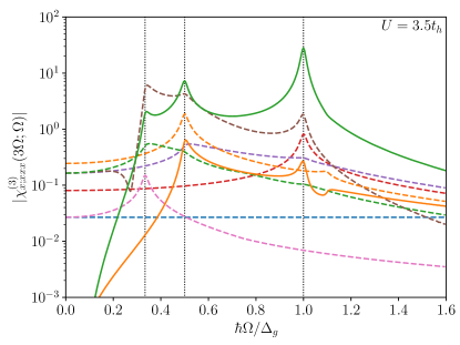
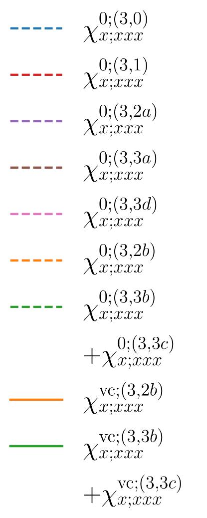
Figure 10: THG susceptibility decomposed into the bare susceptibilities and vertex corrections, where $U=3.5t_{h}$, $D=\Delta_{0}-\Delta_{1}=3.8t_{h}$, and $\eta=0.01\Delta_{g}$ are assumed. The vertical dotted lines indicate $\hbar\Omega=\Delta_{g}/3$, $\Delta_{g}/2$, and $\Delta_{g}$.

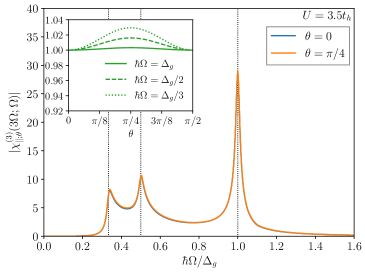
Figure 11: THG susceptibility $|\chi^{(3)}_{\parallel,\theta}(3\Omega;\Omega)|$ at $\theta=0$ and $\pi/4$, where $U=3.5t_{h}$, $D=\Delta_{0}-\Delta_{1}=3.8t_{h}$, and $\eta=0.01\Delta_{g}$ are used. The vertical dotted lines indicate $\hbar\Omega=\Delta_{g}/3$, $\Delta_{g}/2$, and $\Delta_{g}$. Inset: Polarization dependence of the normalized $|\chi^{(3)}_{\parallel,\theta}(3\Omega;\Omega)|$ at $\hbar\Omega=\Delta_{g}/3$, $\Delta_{g}/2$, and $\Delta_{g}$, where the susceptibilities are normalized to their values at $\theta=0$.

E Polarization dependence

Here we show the polarization dependence of the THG susceptibility. When the external field

$$\bm{A}(\Omega)=A(\Omega)(\cos\theta\,\bm{e}_{x}+\sin\theta\,\bm{e}_{y})=A(\Omega)\hat{\bm{n}}^{(\theta)}$$ (105)

is applied, the THG susceptibility parallel to the polarization direction $\hat{\bm{n}}^{(\theta)}$ is given by

$$\chi^{(3)}_{\parallel,\theta}(3\Omega;\Omega)=\sum_{\mu,\mu_{1},\mu_{2},\mu_{3}}\chi^{(3)}_{\mu;\mu_{1}\mu_{2}\mu_{3}}(3\Omega;\Omega)n_{\mu}^{(\theta)}n_{\mu_{1}}^{(\theta)}n_{\mu_{2}}^{(\theta)}n_{\mu_{3}}^{(\theta)},$$ (106)

where $\theta$ is the angle with respect to the $x$ axis, and $n_{x}^{(\theta)}=\cos\theta$ and $n_{y}^{(\theta)}=\sin\theta$.

Figure 11 shows the polarization dependence of the THG susceptibility $|\chi^{(3)}_{\parallel,\theta}(3\Omega;\Omega)|$. Even when the incident light is polarized along the $\theta=\pi/4$ direction, $\chi^{(3)}_{\parallel,\theta}(3\Omega;\Omega)$ retains the main features of the THG susceptibility observed at $\theta=0$. The difference in $|\chi^{(3)}_{\parallel,\theta}(3\Omega;\Omega)|$ at $\hbar\Omega=\Delta_{g}/3$ is less than 4% and the others are smaller than that (see the inset of Fig. 11). In particular, $|\chi^{(3)}_{\parallel,\theta}(3\Omega;\Omega)|$ at $\hbar\Omega=\Delta_{g}$ is almost flat with respect to $\theta$. Therefore, the polarization dependence of THG is small in the EI.

References

- Basov et al. (2011) D. N. Basov, R. D. Averitt, D. van der Marel, M. Dressel, and K. Haule, Rev. Mod. Phys., 83, 471 (2011).
- Giannetti et al. (2016) C. Giannetti, M. Capone, D. Fausti, M. Fabrizio, F. Parmigiani, and D. Mihailovic, Adv. Phys., 65, 58 (2016).
- Mott (1961) N. F. Mott, Philos. Mag., 6, 287 (1961).
- (4) R. S. Knox, Theory of Excitons, Solid State Physics, edited by F. Seitz and D. Turnbull (Academic Press, New York, 1963), p. 100.
- Des Cloizeaux (1965) J. Des Cloizeaux, J. Phys. Chem. Solids, 26, 259 (1965), ISSN 0022-3697.
- Keldysh and Kopeav (1965) L. V. Keldysh and Y. V. Kopeav, Sov. Phys. Solid State, 6, 2219 (1965).
- Jérome et al. (1967) D. Jérome, T. M. Rice, and W. Kohn, Phys. Rev., 158, 462 (1967).
- Halperin and Rice (1968) B. I. Halperin and T. M. Rice, Rev. Mod. Phys., 40, 755 (1968).
- Kuneš (2015) J. Kuneš, J. Phys.: Condens. Matter, 27, 333201 (2015).
- Lu et al. (2017) Y. F. Lu, H. Kono, T. I. Larkin, A. W. Rost, T. Takayama, A. V. Boris, B. Keimer, and H. Takagi, Nat. Commun., 8, 14408 (2017).
- Kogar et al. (2017) A. Kogar, M. S. Rak, S. Vig, A. A. Husain, F. Flicker, Y. I. Joe, L. Venema, G. J. MacDougall, T. C. Chiang, E. Fradkin, J. van Wezel, and P. Abbamonte, Science, 358, 1314 (2017), ISSN 0036-8075.
- (12) Y. Jia, P. Wang, C.-L. Chiu, Z. Song, G. Yu, B. Jäck, S. Lei, S. Klemenz, F. A. Cevallos, M. Onyszczak, N. Fishchenko, X. Liu, G. Farahi, F. Xie, Y. Xu, K. Watanabe, T. Taniguchi, B. A. Bernevig, R. J. Cava, L. M. Schoop, A. Yazdani, and S. Wu, arXiv:2010.05390 .
- Batyev and Borisyuk (1980) E. Batyev and V. Borisyuk, JETP Lett, 32, 395 (1980).
- Portengen et al. (1996) T. Portengen, T. Östreich, and L. J. Sham, Phys. Rev. B, 54, 17452 (1996).
- Batista (2002) C. D. Batista, Phys. Rev. Lett., 89, 166403 (2002).
- Kaneko and Ohta (2016) T. Kaneko and Y. Ohta, Phys. Rev. B, 94, 125127 (2016).
- Kaneko et al. (2021) T. Kaneko, Z. Sun, Y. Murakami, D. Golež, and A. J. Millis, Phys. Rev. Lett., 127, 127402 (2021).
- Brydon and Timm (2009) P. M. R. Brydon and C. Timm, Phys. Rev. B, 80, 174401 (2009).
- Kaneko et al. (2012) T. Kaneko, K. Seki, and Y. Ohta, Phys. Rev. B, 85, 165135 (2012).
- Kuneš and Augustinský (2014) J. Kuneš and P. Augustinský, Phys. Rev. B, 90, 235112 (2014).
- Nasu et al. (2016) J. Nasu, T. Watanabe, M. Naka, and S. Ishihara, Phys. Rev. B, 93, 205136 (2016).
- Yamaguchi et al. (2017) T. Yamaguchi, K. Sugimoto, and Y. Ohta, J. Phys. Soc. Jpn., 86, 043701 (2017).
- Geffroy et al. (2019) D. Geffroy, J. Kaufmann, A. Hariki, P. Gunacker, A. Hausoel, and J. Kuneš, Phys. Rev. Lett., 122, 127601 (2019).
- Nishida et al. (2019) H. Nishida, S. Miyakoshi, T. Kaneko, K. Sugimoto, and Y. Ohta, Phys. Rev. B, 99, 035119 (2019).
- Wang et al. (2019) R. Wang, O. Erten, B. Wang, and D. Y. Xing, Nat. Commun., 10, 210 (2019).
- Perfetto and Stefanucci (2020) E. Perfetto and G. Stefanucci, Phys. Rev. Lett., 125, 106401 (2020).
- Varsano et al. (2020) D. Varsano, M. Palummo, E. Molinari, and M. Rontani, Nat. Nanotechnol., 15, 367 (2020).
- Sun and Millis (2021) Z. Sun and A. J. Millis, Phys. Rev. Lett., 126, 027601 (2021).
- Liu et al. (2021) Z.-R. Liu, L.-H. Hu, C.-Z. Chen, B. Zhou, and D.-H. Xu, Phys. Rev. B, 103, L201115 (2021).
- Sun et al. (2021) Z. Sun, T. Kaneko, D. Golež, and A. J. Millis, Phys. Rev. Lett., 127, 127702 (2021).
- Littlewood et al. (2004) P. B. Littlewood, P. R. Eastham, J. M. J. Keeling, F. M. Marchetti, B. D. Simons, and M. H. Szymanska, J. Phys. Condens. Matter, 16, S3597 (2004).
- Bronold and Fehske (2006) F. X. Bronold and H. Fehske, Phys. Rev. B, 74, 165107 (2006).
- Ihle et al. (2008) D. Ihle, M. Pfafferott, E. Burovski, F. X. Bronold, and H. Fehske, Phys. Rev. B, 78, 193103 (2008).
- Seki et al. (2011) K. Seki, R. Eder, and Y. Ohta, Phys. Rev. B, 84, 245106 (2011).
- Zenker et al. (2012) B. Zenker, D. Ihle, F. X. Bronold, and H. Fehske, Phys. Rev. B, 85, 121102 (2012).
- Cercellier et al. (2007) H. Cercellier, C. Monney, F. Clerc, C. Battaglia, L. Despont, M. G. Garnier, H. Beck, P. Aebi, L. Patthey, H. Berger, and L. Forró, Phys. Rev. Lett., 99, 146403 (2007).
- Monney et al. (2009) C. Monney, H. Cercellier, F. Clerc, C. Battaglia, E. F. Schwier, C. Didiot, M. G. Garnier, H. Beck, P. Aebi, H. Berger, L. Forró, and L. Patthey, Phys. Rev. B, 79, 045116 (2009).
- Kaneko et al. (2018) T. Kaneko, Y. Ohta, and S. Yunoki, Phys. Rev. B, 97, 155131 (2018).
- Wakisaka et al. (2009) Y. Wakisaka, T. Sudayama, K. Takubo, T. Mizokawa, M. Arita, H. Namatame, M. Taniguchi, N. Katayama, M. Nohara, and H. Takagi, Phys. Rev. Lett., 103, 026402 (2009).
- Kaneko et al. (2013) T. Kaneko, T. Toriyama, T. Konishi, and Y. Ohta, Phys. Rev. B, 87, 035121 (2013a).
- Kaneko et al. (2013) T. Kaneko, T. Toriyama, T. Konishi, and Y. Ohta, Phys. Rev. B, 87, 199902 (2013b).
- Sugimoto et al. (2018) K. Sugimoto, S. Nishimoto, T. Kaneko, and Y. Ohta, Phys. Rev. Lett., 120, 247602 (2018).
- Lee et al. (2019) J. Lee, C.-J. Kang, M. J. Eom, J. S. Kim, B. I. Min, and H. W. Yeom, Phys. Rev. B, 99, 075408 (2019).
- Matsubayashi et al. (2021) K. Matsubayashi, H. Okamura, T. Mizokawa, N. Katayama, A. Nakano, H. Sawa, T. Kaneko, T. Toriyama, T. Konishi, Y. Ohta, H. Arima, R. Yamanaka, A. Hisada, T. Okada, Y. Ikemoto, T. Moriwaki, K. Munakata, A. Nakao, M. Nohara, Y. Lu, H. Takagi, and Y. Uwatoko, J. Phys. Soc. Jpn., 90, 074706 (2021).
- Fukutani et al. (2021) K. Fukutani, R. Stania, C. Il Kwon, J. S. Kim, K. J. Kong, J. Kim, and H. W. Yeom, Nat. Phys., 17, 1024 (2021).
- Wang et al. (2021) P. Wang, G. Yu, Y. Jia, M. Onyszczak, F. A. Cevallos, S. Lei, S. Klemenz, K. Watanabe, T. Taniguchi, R. J. Cava, L. M. Schoop, and S. Wu, Nature, 589, 225 (2021).
- Lee (2021) P. A. Lee, Phys. Rev. B, 103, L041101 (2021).
- Mor et al. (2017) S. Mor, M. Herzog, D. Golež, P. Werner, M. Eckstein, N. Katayama, M. Nohara, H. Takagi, T. Mizokawa, C. Monney, and J. Stähler, Phys. Rev. Lett., 119, 086401 (2017).
- Mor et al. (2018) S. Mor, M. Herzog, J. Noack, N. Katayama, M. Nohara, H. Takagi, A. Trunschke, T. Mizokawa, C. Monney, and J. Stähler, Phys. Rev. B, 97, 115154 (2018).
- Werdehausen et al. (2018) D. Werdehausen, T. Takayama, M. Höppner, G. Albrecht, A. W. Rost, Y. Lu, D. Manske, H. Takagi, and S. Kaiser, Sci. Adv., 4 (2018).
- Okazaki et al. (2018) K. Okazaki, Y. Ogawa, T. Suzuki, T. Yamamoto, T. Someya, S. Michimae, M. Watanabe, Y. Lu, M. Nohara, H. Takagi, N. Katayama, H. Sawa, M. Fujisawa, T. Kanai, N. Ishii, J. Itatani, T. Mizokawa, and S. Shin, Nat. Commun., 9, 4322 (2018).
- Ning et al. (2020) H. Ning, O. Mehio, M. Buchhold, T. Kurumaji, G. Refael, J. G. Checkelsky, and D. Hsieh, Phys. Rev. Lett., 125, 267602 (2020).
- Kim et al. (2020) M.-J. Kim, A. Schulz, T. Takayama, M. Isobe, H. Takagi, and S. Kaiser, Phys. Rev. Research, 2, 042039 (2020).
- Kim et al. (2021) K. Kim, H. Kim, J. Kim, C. Kwon, J. S. Kim, and B. J. Kim, Nat. Commun., 12, 1969 (2021).
- Volkov et al. (2021) P. A. Volkov, M. Ye, H. Lohani, I. Feldman, A. Kanigel, and G. Blumberg, npj Quantum Mater., 6, 52 (2021).
- Ye et al. (2021) M. Ye, P. A. Volkov, H. Lohani, I. Feldman, M. Kim, A. Kanigel, and G. Blumberg, Phys. Rev. B, 104, 045102 (2021).
- Bretscher et al. (2021) H. M. Bretscher, P. Andrich, P. Telang, A. Singh, L. Harnagea, A. K. Sood, and A. Rao, Nat. Commun., 12, 1699 (2021a).
- Suzuki et al. (2021) T. Suzuki, Y. Shinohara, Y. Lu, M. Watanabe, J. Xu, K. L. Ishikawa, H. Takagi, M. Nohara, N. Katayama, H. Sawa, M. Fujisawa, T. Kanai, J. Itatani, T. Mizokawa, S. Shin, and K. Okazaki, Phys. Rev. B, 103, L121105 (2021).
- Saha et al. (2021) T. Saha, D. Golež, G. De Ninno, J. Mravlje, Y. Murakami, B. Ressel, M. Stupar, and P. R. Ribič, Phys. Rev. B, 103, 144304 (2021).
- Bretscher et al. (2021) H. M. Bretscher, P. Andrich, Y. Murakami, D. Golež, B. Remez, P. Telang, A. Singh, L. Harnagea, N. R. Cooper, A. J. Millis, P. Werner, A. K. Sood, and A. Rao, Sci. Adv., 7, eabd6147 (2021b).
- (61) E. Baldini, A. Zong, D. Choi, C. Lee, M. H. Michael, L. Windgaetter, I. I. Mazin, S. Latini, D. Azoury, B. Lv, A. Kogar, Y. Wang, Y. Lu, T. Takayama, H. Takagi, A. J. Millis, A. Rubio, E. Demler, and N. Gedik, arXiv:2007.02909 .
- (62) P. A. Volkov, M. Ye, H. Lohani, I. Feldman, A. Kanigel, and G. Blumberg, arXiv:2104.07032 .
- Pekker and Varma (2015) D. Pekker and C. Varma, Annu. Rev. Condens. Matter Phys., 6, 269 (2015).
- Tsuji and Aoki (2015) N. Tsuji and H. Aoki, Phys. Rev. B, 92, 064508 (2015).
- Cea et al. (2016) T. Cea, C. Castellani, and L. Benfatto, Phys. Rev. B, 93, 180507 (2016).
- Tsuji et al. (2016) N. Tsuji, Y. Murakami, and H. Aoki, Phys. Rev. B, 94, 224519 (2016).
- Tsuji and Nomura (2020) N. Tsuji and Y. Nomura, Phys. Rev. Research, 2, 043029 (2020).
- Schwarz and Manske (2020) L. Schwarz and D. Manske, Phys. Rev. B, 101, 184519 (2020).
- Seibold et al. (2021) G. Seibold, M. Udina, C. Castellani, and L. Benfatto, Phys. Rev. B, 103, 014512 (2021).
- Matsunaga et al. (2014) R. Matsunaga, N. Tsuji, H. Fujita, A. Sugioka, K. Makise, Y. Uzawa, H. Terai, Z. Wang, H. Aoki, and R. Shimano, Science, 345, 1145 (2014), ISSN 0036-8075.
- Matsunaga et al. (2017) R. Matsunaga, N. Tsuji, K. Makise, H. Terai, H. Aoki, and R. Shimano, Phys. Rev. B, 96, 020505 (2017).
- Matsunaga and Shimano (2017) R. Matsunaga and R. Shimano, Phys. Scr., 92, 024003 (2017).
- Shimano and Tsuji (2020) R. Shimano and N. Tsuji, Annu. Rev. Condens. Matter Phys., 11, 103 (2020).
- Chu et al. (2020) H. Chu, M.-J. Kim, K. Katsumi, S. Kovalev, R. D. Dawson, L. Schwarz, N. Yoshikawa, G. Kim, D. Putzky, Z. Z. Li, H. Raffy, S. Germanskiy, J.-C. Deinert, N. Awari, I. Ilyakov, B. Green, M. Chen, M. Bawatna, G. Cristiani, G. Logvenov, Y. Gallais, A. V. Boris, B. Keimer, A. P. Schnyder, D. Manske, M. Gensch, Z. Wang, R. Shimano, and S. Kaiser, Nat. Commun., 11, 1793 (2020).
- Murakami et al. (2017) Y. Murakami, D. Golež, M. Eckstein, and P. Werner, Phys. Rev. Lett., 119, 247601 (2017).
- Murakami et al. (2020) Y. Murakami, D. Golež, T. Kaneko, A. Koga, A. J. Millis, and P. Werner, Phys. Rev. B, 101, 195118 (2020).
- Golež et al. (2020) D. Golež, Z. Sun, Y. Murakami, A. Georges, and A. J. Millis, Phys. Rev. Lett., 125, 257601 (2020).
- Tanaka et al. (2018) Y. Tanaka, M. Daira, and K. Yonemitsu, Phys. Rev. B, 97, 115105 (2018).
- Kaneko et al. (2013) T. Kaneko, S. Ejima, H. Fehske, and Y. Ohta, Phys. Rev. B, 88, 035312 (2013c).
- Ejima et al. (2014) S. Ejima, T. Kaneko, Y. Ohta, and H. Fehske, Phys. Rev. Lett., 112, 026401 (2014).
- Seki et al. (2014) K. Seki, Y. Wakisaka, T. Kaneko, T. Toriyama, T. Konishi, T. Sudayama, N. L. Saini, M. Arita, H. Namatame, M. Taniguchi, N. Katayama, M. Nohara, H. Takagi, T. Mizokawa, and Y. Ohta, Phys. Rev. B, 90, 155116 (2014).
- Hamada et al. (2017) K. Hamada, T. Kaneko, S. Miyakoshi, and Y. Ohta, J. Phys. Soc. Jpn., 86, 074709 (2017).
- Kadosawa et al. (2020) M. Kadosawa, S. Nishimoto, K. Sugimoto, and Y. Ohta, J. Phys. Soc. Jpn., 89, 053706 (2020).
- Tanabe et al. (2018) T. Tanabe, K. Sugimoto, and Y. Ohta, Phys. Rev. B, 98, 235127 (2018).
- Fujiuchi et al. (2019) R. Fujiuchi, T. Kaneko, Y. Ohta, and S. Yunoki, Phys. Rev. B, 100, 045121 (2019).
- Aoki et al. (2014) H. Aoki, N. Tsuji, M. Eckstein, M. Kollar, T. Oka, and P. Werner, Rev. Mod. Phys., 86, 779 (2014).
- Parker et al. (2019) D. E. Parker, T. Morimoto, J. Orenstein, and J. E. Moore, Phys. Rev. B, 99, 045121 (2019).
- (88) While we assume the order parameter at finite temperature in the 2D model with the continuous symmetry, the ordered states in the quasi-2D EI candidates may be characterized by the broken discrete symmetries due to additional factors (e.g. electron-phonon coupling) Zenker et al. (2014); Kaneko et al. (2015), so that we expect that the tendencies of our main results are comparable with THG in the candidate materials.
- Di Salvo et al. (1976) F. J. Di Salvo, D. E. Moncton, and J. V. Waszczak, Phys. Rev. B, 14, 4321 (1976).
- Di Salvo et al. (1986) F. Di Salvo, C. Chen, R. Fleming, J. Waszczak, R. Dunn, S. Sunshine, and J. A. Ibers, J. Less-Common Met., 116, 51 (1986), ISSN 0022-5088.
- Holt et al. (2001) M. Holt, P. Zschack, H. Hong, M. Y. Chou, and T.-C. Chiang, Phys. Rev. Lett., 86, 3799 (2001).
- Nakano et al. (2018) A. Nakano, T. Hasegawa, S. Tamura, N. Katayama, S. Tsutsui, and H. Sawa, Phys. Rev. B, 98, 045139 (2018).
- Larkin et al. (2017) T. I. Larkin, A. N. Yaresko, D. Pröpper, K. A. Kikoin, Y. F. Lu, T. Takayama, Y.-L. Mathis, A. W. Rost, H. Takagi, B. Keimer, and A. V. Boris, Phys. Rev. B, 95, 195144 (2017).
- Larkin et al. (2018) T. I. Larkin, R. D. Dawson, M. Höppner, T. Takayama, M. Isobe, Y.-L. Mathis, H. Takagi, B. Keimer, and A. V. Boris, Phys. Rev. B, 98, 125113 (2018).
- Binosi and Theußl (2004) D. Binosi and L. Theußl, Comp. Phys. Comm., 161, 76 (2004), ISSN 0010-4655.
- Passos et al. (2018) D. J. Passos, G. B. Ventura, J. M. V. P. Lopes, J. M. B. L. d. Santos, and N. M. R. Peres, Phys. Rev. B, 97, 235446 (2018).
- Holder et al. (2020) T. Holder, D. Kaplan, and B. Yan, Phys. Rev. Research, 2, 033100 (2020).
- Zenker et al. (2014) B. Zenker, H. Fehske, and H. Beck, Phys. Rev. B, 90, 195118 (2014).
- Kaneko et al. (2015) T. Kaneko, B. Zenker, H. Fehske, and Y. Ohta, Phys. Rev. B, 92, 115106 (2015).