Polarizing electron spins with a superconducting flux qubit

Abstract

Electron spin resonance (ESR) is a useful tool to investigate properties of materials in magnetic fields where high spin polarization of target electron spins is required in order to obtain high sensitivity. However, the smaller magnetic fields becomes, the more difficult high polarization is passively obtained by thermalization. Here, we propose to employ a superconducting flux qubit (FQ) to polarize electron spins actively. We have to overcome a large energy difference between the FQ and electron spins for efficient energy transfer among them. For this purpose, we adopt a spin-lock technique on the FQ where the Rabi frequency associated with the spin-locking can match the resonance (Larmor) one of the electron spins. We find that adding dephasing on the spins is beneficial to obtain high polarization of them, because otherwise the electron spins are trapped in dark states that cannot be coupled with the FQ. We show that our scheme can achieve high polarization of electron spins in realistic experimental conditions.

I Introduction

Increasing attention has been paid to electron spin resonance (ESR) due to an excellent sensitivity compared with that of nuclear magnetic resonance (NMR). An improvement of the ESR sensitivity is important for practical applications. Therefore, superconducting circuits have often been used to detect the small number of electron spins [1, 2, 3, 4, 5, 6, 7, 8]. By using a superconducting resonator, it is possible to measure only $12$ spins with 1 s measurement time where the detection volume is around 6fl [9] where the frequency of the superconducting resonator is fixed. It is favorable to sweep not only the microwave frequency but also the magnetic field to investigate complicated spin systems. For this purpose, we could use a waveguide [10], a frequency tunable resonator [11], or a direct current-superconducting quantum interference device (dcSQUID) [2, 12]. Among these approaches, a superconducting flux qubit (FQ) is promising and has already achieved a sensitivity of $20$ spins/Hz^1/2 with a sensing volume of 6 fl for the ESR [13].

It is worth mentioning that the FQ cannot work if we apply high magnetic fields, and so the applied field should be smaller than 10 mT [2]. One of the problems in FQ-ESR measurements is a low polarization of target electrons especially when they are in a low magnetic field. A typical thermal energy $\sim k_{\rm B}T$ ($k_{\rm B}$: the Boltzmann constant and T: temperature) at mK temperatures is around hundreds of MHz in frequency unit, while the typical magnetic energy of the electron spins $\sim\mu_{\rm B}B$ ($\mu_{\rm B}$: the Bohr magneton constant and $B$: flux density in T unit) in a small field of few mT is about tens of MHz. This implies that the electron spins cannot be fully polarized in these conditions and that the sensitivity of ESR is deteriorated. Note that high spin polarization of target electrons is required in order to obtain high sensitivity [14]. A Purcell effect [15] was recently employed to polarize electron spins with a superconducting cavity [16]. However, this is not applicable to the case when electron spins are placed in a low magnetic field because of a large energy difference between the cavity and electron spins. Moreover, a thermal relaxation time of electron spins becomes larger at lower temperature, and thus it is difficult to polarize them [17, 18, 19, 20].

Here, we propose to employ a FQ for not only detecting but also polarizing electron spins. The main idea is that the energy relaxation time of the FQ is much shorter than that of the electron spins, and so we can efficiently emit the energy of the electron spin to the environment by using a coupling between the FQ and electron spins. We adopt a spin-lock technique where the Rabi frequency of the FQ in a rotating frame associated with the spin-locking matches with the resonance (Larmor) frequency of the electron spins in a low magnetic field [21]. The important difference from the polarization with a Purcell effect [16] is that the Rabi frequency can be much smaller than the resonance one of the FQ. By using a long-lived FQ such as a capacitively shunted FQ whose coherence time is around tens of micro seconds [22, 23, 24], the Rabi frequency can be reduced to hundreds of kHz. With these properties, one may overcome the energy scale mismatch between a FQ and electron spins, and thus the efficient polarization of the electron spins becomes possible.

This paper is organized as follows. § II illustrates our setup and proposal with analytical discussion on a simplified model. We show our numerical simulations with realistic experimental parameters in § III for demonstrating its experiment feasibility. We conclude this paper in § IV.

II Theory

We here propose to employ a Hartmann-Hahn (H-H) resonance [21] to polarize electron spins with a FQ. The H-H resonance has been applied to polarize environmental spins by using nitrogen vacancy (NV) centers in diamond [25, 26]. Our proposal is expected to polarize far more electron spins than the case of the NV center in diamond, because the size of the FQ is of the order of micrometers while that of the NV center is of the order of angstroms.

We discuss a simplified model in order to illustrate our proposal after introducing a Hamiltonian and Lindbladian that govern the electron spins and FQ.

II.1 Model

The Hamiltonian of a FQ coupled to $M$ electron spins (labeled with $k=1\sim M$) is described as follows.

$$H = H_{\rm{FQ}}+H_{\rm{spin}}+H_{\rm{I}},$$

where $H_{\rm{FQ}}$, $H_{\rm{spin}}$, and $H_{\rm{I}}$ denote the Hamiltonian of the FQ, spins, and interaction between them. $H_{\rm{FQ}}$ is given as

$$H_{\rm{FQ}} = \frac{\epsilon}{2}Z+\frac{\Delta}{2}X+\lambda Y\cos\omega t,$$

where $\epsilon$ denotes the energy bias, $\Delta$ the tunneling energy, $\omega$ the frequency of the microwave, and $\lambda$ the strength of the microwave. $X$, $Y$, and $Z$ are standard Pauli matrices acting on the FQ. It is convenient for us to change the notation, and we rewrite $H_{\rm{FQ}}$ as follows.

$$H_{\rm{FQ}} = \frac{\epsilon}{2}\sigma^{(0)}_{x}+\frac{\Delta}{2}\sigma^{(0)}_{y}+\lambda\sigma_{z}^{(0)}\cos\omega t,$$

where we change $X$, $Y$, and $Z$ to $\sigma^{(0)}_{y}$, $\sigma^{(0)}_{z}$ and $\sigma^{(0)}_{x}$, respectively. 0 denotes the 0th qubit in our system. $H_{\rm{spin}}$ and $H_{\rm{I}}$ are given as

$$H_{\rm{spin}} = \sum_{k=1}^{M}\omega_{k}\sigma_{z}^{(k)},$$

$$H_{\rm{I}} = \sum_{k=1}^{M}g_{k}\sigma^{(0)}_{x}\sigma_{x}^{(k)},$$

where $\omega_{k}$ denotes the resonance frequency of the $k$-th spin and $g_{k}$ the coupling strength between the FQ and the $k$-th spin. By going to a rotating frame with a frequency of $\omega=\sqrt{\epsilon^{2}+\Delta^{2}}$ of the FQ, we obtain the following Hamiltonian with a rotating wave approximation with a condition of $\epsilon\gg\Delta$

$$H\simeq\frac{\lambda}{2}\sigma^{(0)}_{z}+\sum_{k=1}^{M}\omega_{k}\sigma_{z}^{(k)}+\sum_{k=1}^{M}g_{k}\sigma^{(0)}_{x}\sigma_{x}^{(k)}.$$ (1)

We obtain the following effective Hamiltonian in a rotating frame of which frequency is $\displaystyle\omega_{\rm avg}=\frac{1}{M}\sum_{k}\omega_{k}$ with the rotating wave approximation.

$$H \simeq\sum_{k=1}^{M}\left(\omega_{k}^{\prime}\sigma_{z}^{(k)}+g_{k}\left(\sigma^{(0)}_{+}\sigma_{-}^{(k)}+\sigma^{(0)}_{-}\sigma_{+}^{(k)}\right)\right),$$ (2)

where $\omega_{k}^{\prime}=\omega_{k}-\omega_{\rm avg}$ and $\sigma_{\pm}=\sigma_{x}\pm i\sigma_{y}$. Here, we set $\lambda/2$ to be $\omega_{\rm avg}$.

The energy exchanges occur between the FQ and electron spins during the irradiation of a microwave due to the flip-flop interaction, while there is no coupling between them in the absence of the irradiation due to the energy detuning of $\sqrt{\epsilon^{2}+\Delta^{2}}\gg\omega_{k}$.

We also introduce the Lindblad operator in order to describe the relaxation of the system (= a FQ and spins), as follows.

$${\cal L}[\rho]= \sum_{l=0}^{M}\gamma_{\rm T}^{(l)}\left(\sigma^{(l)}_{z}\rho\sigma^{(l)}_{z}-\rho\right)$$

$$+\sum_{l=0}^{M}\gamma_{\rm L}^{(l)}\left(\sigma^{(l)}_{+}\rho\sigma^{(l)}_{-}+\sigma^{(l)}_{-}\rho\sigma^{(l)}_{+}-\rho\right),$$ (3)

where $\gamma_{\rm T}$ and $\gamma_{\rm L}$ characterize the strengths of transversal and longitudinal relaxations, respectively. Note that the superscript $l$ runs from $0$ to $M$ while $k$ runs from $1$ to $M$. We consider the case when each qubit has a different relaxation parameter labeled with $*^{(l)}$.

A system dynamics is then determined by

$$\frac{d\rho}{dt}=-i[H,\rho]+{\cal L}[\rho],$$ (4)

while the initial state is assumed to be

$$\rho(0)=|0\rangle\langle 0|\otimes\bigotimes^{M}_{k=1}\frac{\sigma_{0}}{2},$$ (5)

where $\sigma_{0}$ is the $2\times 2$ identity matrix. Then, our goal is to obtain

$$\rho({\rm final})=|0\rangle\langle 0|\otimes\bigotimes^{M}_{k=1}|0\rangle\langle 0|,$$ (6)

after some operations.

II.2 Simplified Model

We consider a simplified model where $\omega_{k}$’s and $g_{k}$’s are identical for $k=1\sim M$. Due to this simplification, we can calculate polarization dynamics for a large number of spins. Our procedure consists of two steps, Step I and II. A FQ interacts with the spins and absorbs their entropy in Step I while the spin states are homogenized with a help of dephasing in Step II.

• in Step I

  Let the system develop according to the following simplified Hamiltonian. This is obtained from Eq. (2) by assuming $g_{k}=g$ and $\omega_{k}^{\prime}=0$ for $k=1\sim M$.

  $$H^{\rm I} =g\left(\sigma^{(0)}_{+}S_{-}+\sigma^{(0)}_{-}S_{+}\right),$$ (7)

  $$S_{x,y,z,\pm} =\sum^{M}_{k=1}\sigma^{(k)}_{x,y,z,\pm},$$

  while the Lindbladian (II.1) is simplified as

  $${\cal L}^{\rm I}[\rho]=\gamma\left(\sigma^{(0)}_{z}\rho\sigma^{(0)}_{z}-\rho\right),$$ (8)

  where we assume that only $\gamma_{\rm T}^{(0)}=\gamma\neq 0$ and the other $\gamma_{\rm T}^{(k)}$ and $\gamma_{\rm L}^{(l)}$ are negligible. The only 0th qubit is under influence of dephasing.

  After the dynamics, we initialize the 0th qubit to the ground state $|0\rangle$ without disturbing the others ($k=1\sim M$).

• in Step II

  We decouple the 0th qubit from the others. Therefore, the Hamiltonian is given as,

  $$H^{\rm II} =0,$$ (9)

  while the Lindbladian (II.1) in Step II is simplified as

  $${\cal L}^{\rm II}[\rho]=\sum^{M}_{k=1}\gamma^{\prime}\left(\sigma^{(k)}_{z}\rho\sigma^{(k)}_{z}-\rho\right),$$ (10)

  where we assume that only $\gamma_{\rm T}^{(k)}=\gamma^{\prime}\neq 0$ and the other $\gamma_{\rm T}^{(0)}$ and $\gamma_{\rm L}^{(l)}$ are negligible. All qubits except the 0th one are under influence of the same dephasing.

II.3 Step I

We employ the Young-Yamanouchi basis $|j,m,i\rangle$ [27] in order to represent the spin state. Note that $j=1/2,3/2,\cdots,M/2$ and $|m|\leq j$ (half-integer) for odd $M$ cases while $j=0,1,\cdots,M/2$ and $|m|\leq j$ (integer) for the even $M$ cases. The index $i$ represents the number of ways of composing $n$ qubits to obtain the total angular momentum $j$ and takes $1\sim d_{j}$, where $d_{j}:=(2j+1)M!/(M/2+j+1)!(M/2-j)!$. The action of spin operators $S_{\pm,z}$ is given as follows.

$$S_{+}|j,m,i\rangle =\sqrt{j(j+1)-m(m+1)}|j,m+1,i\rangle,$$

$$S_{-}|j,m,i\rangle =\sqrt{j(j+1)-m(m-1)}|j,m-1,i\rangle,$$

$$\frac{S_{z}}{2}|j,m,i\rangle =m|j,m,i\rangle.$$ (11)

Let us define

$$|a_{jmi}\rangle :=|0\rangle\otimes|j,m,i\rangle,$$

$$|b_{jmi}\rangle :=|1\rangle\otimes|j,m-1,i\rangle.$$ (12)

By using the above bases, the initial state (5) can be rewritten as

$$\rho(0) =\frac{1}{2^{M}}\sum_{j,m,i}|a_{jmi}\rangle\langle a_{jmi}|.$$ (13)

The dynamics of $\rho(t)$ from the above initial state according to Eq. (4) with Eqs. (7) and (8) is easily obtained with the help of Eq. (II.3):

$$\rho(t) =\frac{1}{2^{M}}\sum_{j,m,i}\rho_{jmi}(t),$$

$$\rho_{jmi}(t) :=a_{jmi}(t)|a_{jmi}\rangle\langle a_{jmi}|+b_{jmi}(t)|b_{jmi}\rangle\langle b_{jmi}|$$

$$+c_{jmi}(t)|a_{jmi}\rangle\langle b_{jmi}|+c_{jmi}^{*}(t)|b_{jmi}\rangle\langle a_{jmi}|.$$ (14)

Here the coefficients $a_{jmi}(t)$, $b_{jmi}(t)$, $c_{jmi}(t)$ satisfy the following differential equations,

$$\dot{a}_{jmi}(t)= -2gl_{jm}c_{jmi}^{I}(t),$$

$$\dot{b}_{jmi}(t)= 2gl_{jm}c_{jmi}^{I}(t),$$

$$\dot{c}_{jmi}^{I}(t)= gl_{jm}a_{jmi}(t)-gl_{jm}b_{jmi}(t)-2\gamma c_{jmi}^{I}(t),$$

$$\dot{c}_{jmi}^{R}(t)= -2\gamma c_{jmi}^{R}(t),$$ (15)

where $c^{I~{}(R)}_{jmi}(t)$ is the imaginary (real) part of $c_{jmi}$ and $l_{jm}=\sqrt{j(j+1)-m(m-1)}$. The dynamics of each $\rho_{jmi}(t)$, or the dynamics of $\{a_{jmi}(t),b_{jmi}(t),c_{jmi}(t)\}$, is independent of each other.

Let us now focus on the dynamics of $\rho_{jmi}(t)$ for fixed $j,m,i$. Because the dynamics of $c_{jmi}^{R}(t)$ is decoupled from those of the other variables, we assume that $c_{jmi}$ is pure imaginary from now on. The eigenvalues of this dynamics (= decay rates) are given as

$$0,~{}\frac{-\gamma+\sqrt{\gamma^{2}-(16gl_{jm})^{2}}}{2},~{}\frac{-\gamma-\sqrt{\gamma^{2}-(16gl_{jm})^{2}}}{2}.$$ (16)

The eigenstate corresponding to the eigenvalue 0 is $\frac{1}{2}|a_{jmi}\rangle\langle a_{jmi}|+\frac{1}{2}|b_{jmi}\rangle\langle b_{jmi}|$ and is independent of $\gamma$. Note that this state corresponds to the fully mixed state in the space spanned by $|a_{jmi}\rangle$ and $|b_{jmi}\rangle$, and is stationary.

Let us consider the dynamics of which initial state is given as

$$\rho=\sum_{j,m,i}p_{j,m}|a_{jmi}\rangle\langle a_{jmi}|.$$ (17)

The states at the beginning and the end of Step I + II (and also the initial state) can be always written in the above form as shown below. The reason why $p_{j,m}$ is independent of the index $i$ is that there is no way to control the freedom of $i$ in our protocol and the initial state is also set to be independent of the index $i$. Because the dynamics of each $|a_{jmi}\rangle\langle a_{jmi}|$ is independent of each other, the dynamics from the initial state (17) is simply given as

$$\rho(t)=\sum_{j,m,i}p_{j,m}\rho_{jmi}(t).$$ (18)

Then, it is assumed that we can wait until the above dynamics converges. After that, we obtain the stationary state of which density matrix $\rho_{\rm st}$ is given as

$$\rho_{\rm st} =\sum_{j,m,i}\frac{p_{j,m}}{2}(|a_{jmi}\rangle\langle a_{jmi}|+|b_{jmi}\rangle\langle b_{jmi}|).$$ (19)

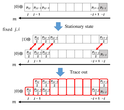
Figure 1: (color on line) Schematic picture of Dynamics of Step I which consists of “obtaining stationary state, $\rho\rightarrow\rho_{\rm st}$” and “trace out” processes. In the $\rho\rightarrow\rho_{\rm st}$ process, we have initially $\rho=\sum_{j,m,i}p_{j,m}|a_{jmi}\rangle\langle a_{jmi}|$ where $|a_{jmi}\rangle=|0\rangle\otimes|j,m,i\rangle$, which is illustrated in the upper row. When the system becomes stationary state, we obtain $\rho_{\rm st}=\sum_{j,m,i}\frac{p_{j,m}}{2}(|a_{jmi}\rangle\langle a_{jmi}|+|b_{jmi}\rangle\langle b_{jmi}|)$ where $|b_{jmi}\rangle=|1\rangle\otimes|j,m-1,i\rangle$, and we intuitively show this in the middle row. When the FQ is isolated from the $k$th qubits and initialized at the end of Step I, we obtain $\rho^{\rm I}=\sum_{j,m,i}p^{\prime}_{j,m}|a_{jmi}\rangle\langle a_{jmi}|$, as shown in the bottom row. The gray zones represent the dark state.

We then cut the interaction between the 0th qubit and the others, and initialize the 0th qubit state to the ground state $|0\rangle$. The final total density matrix is given as

$$\rho^{\rm I} =|0\rangle\langle 0|\otimes{\rm Tr}_{0}(\rho_{\rm st})=\sum_{j,m,i}p^{\prime}_{j,m}|a_{jmi}\rangle\langle a_{jmi}|,$$ (20)

where ${\rm Tr}_{0}$ denotes that only the 0th qubit degrees of freedom is traced out. By simple calculations, we obtain

$$p^{\prime}_{j,j} =\frac{p_{j,j}}{2},$$

$$p^{\prime}_{j,m} =\frac{p_{j,m}}{2}+\frac{p_{j,m+1}}{2},~{}~{}m\neq j,-j$$

$$p^{\prime}_{j,-j} =p_{j,-j}+\frac{p_{j,-j+1}}{2}.$$ (21)

Thus, the repetition of Step I can be completely represented by the above update rule (21). See Fig. 1.

The above processes (dynamics + trace out + initialization) is called Step I hereinafter. Fig. 2 shows the global view of the whole density matrix dynamics during Step I.

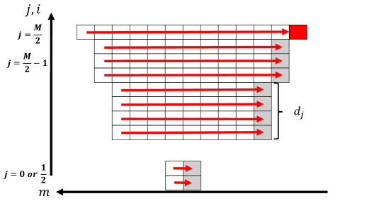
Figure 2: (color online) Global view of the repetitive application of the update rule (21) of Step I. The states of $|j,m,i\rangle$ converges to the states of $|j,-j,i\rangle$. The red zone represents the target polarized state where every qubit is in the ground state.

II.4 Step II

Even when we repeat the Step I, we cannot polarize all qubits, because of the existence of the so-called dark states of $|j,-j,i\rangle$ [28, 29, 30, 31, 32, 33, 34, 35]. By the repetitive application of the step I, the population of each basis $|a_{jmi}\rangle\langle a_{jmi}|$ in Eq. (17) except that of the dark states converges to zero and thus the populations will be accumulated onto these dark states. At the infinite repetition limit, the density matrix is given as

$$\rho=\sum_{j,m,i}\delta_{m,-j}p^{\infty}_{j,-j}|a_{jmi}\rangle\langle a_{jmi}|,~{}~{}p^{\infty}_{j,-j}:=\frac{2j+1}{2^{M}}.$$ (22)

Therefore, we cannot achieve perfect polarization only by Step I.

To overcome this problem, in Step II, we apply dephasing noise to the qubits ($k=1\sim M$) of which state is given by $\rho^{\rm I}$ (Eq. (20)) according to Eq. (10), and we wait until the dynamics converges. We will prove that the density matrix after Step II is given as

$$\rho^{\rm II} =\sum_{j,m,i}P_{m}|a_{jmi}\rangle\langle a_{jmi}|.$$ (23)

The dephasing remove the $j$ dependence in the probability of $|a_{jmi}\rangle\langle a_{jmi}|$. Note that the density matrix given in Eq. (23) is also a special case of Eq. (17).

We first introduce $\rho_{j,m}$ which is given as

$$\rho_{j,m}:=\sum^{d_{j}}_{i=1}|a_{jmi}\rangle\langle a_{jmi}|.$$ (24)

Let us denote the operation of Step II by ${\cal E}_{\rm II}$. Then the dynamics of Step II is given as

$$\rho^{\rm II} ={\cal E}_{\rm II}(\rho_{\rm I})=\sum_{j,m}p^{\prime}_{j,m}\Bigl{(}{\cal E}_{\rm II}(\rho_{j,m})\Bigr{)}.$$ (25)

The action of ${\cal E}_{\rm II}$ is written as

$${\cal E}_{\rm II}(\rho_{j,m})=\frac{d_{j}}{{}_{M}C_{m+M/2}}\sum_{s=|m|}^{M/2}\sum^{d_{s}}_{i=1}|a_{smi}\rangle\langle a_{smi}|,$$ (26)

which is shown in Appendix.

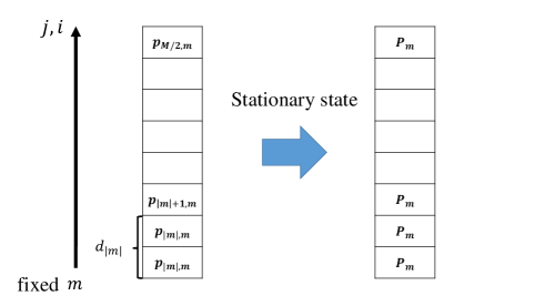
Figure 3: (color online) Step II can be regarded as a process of averaging of $p_{j,m}$ about $j$ and $i$ for fixed $m$. After Step II, the population of $|j,m,i\rangle$ in the density matrix does not depend on $j$.

After showing the $\sum$’s in $\rho^{\rm I}$ explicitly, we transform $\rho^{\rm I}$ as follows.

$$\rho^{\rm II}$$

$$=\sum_{m=-M/2}^{M/2}\sum^{M/2}_{j=|m|}p^{\prime}_{j,m}\left(\frac{d_{j}}{{}_{M}C_{m+M/2}}\sum_{s=|m|}^{M/2}\sum^{d_{s}}_{i=1}|a_{smi}\rangle\langle a_{smi}|\right)$$

$$=\sum_{m=-M/2}^{M/2}\left(\sum^{M/2}_{j=|m|}p^{\prime}_{j,m}\frac{d_{j}}{{}_{M}C_{m+M/2}}\right)\sum_{s=|m|}^{M/2}\sum^{d_{s}}_{i=1}|a_{smi}\rangle\langle a_{smi}|$$

$$=\sum_{m=-M/2}^{M/2}P_{m}\sum^{M/2}_{s=|m|}\sum^{d_{s}}_{i=1}|a_{smi}\rangle\langle a_{smi}|$$

$$=\sum_{j,m,i}P_{m}|a_{jmi}\rangle\langle a_{jmi}|,$$ (27)

where $P_{m}$ is given as

$$P_{m} =\sum^{M/2}_{j=|m|}p^{\prime}_{j,m}\frac{d_{j}}{{}_{M}C_{m+\frac{M}{2}}}$$

$$=\frac{1}{{}_{M}C_{m+\frac{M}{2}}}\sum^{M/2}_{j=|m|}\sum^{d_{j}}_{i=1}p^{\prime}_{j,m}.$$ (28)

Because the number of orthogonal states $|a_{jmi}\rangle$ for each $m$ is ${}_{M}C_{m+\frac{M}{2}}$, this process can be considered as an averaging process of $p^{\prime}_{j,m}$ in $\rho^{\rm I}$ for a fixed $m$. (See Fig. 3 for intuitive explanation of the Step II.) Thus, Step II can be totally represented by the update rule,

$$p^{\prime}_{j,m}\rightarrow P_{m}.$$ (29)

Figure 4 shows the schematic view of the whole density matrix dynamics after Step II.

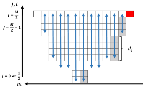
Figure 4: (color online) Global view of the update rule (29) of Step II, which is regarded as averaging of the population of $|j,m,i\rangle$ about $j$ and $i$ for fixed $m$. The blue arrow in the figure denotes such an averaging.

II.5 Step I + Step II

It is possible to polarize the qubits to ground states by combining Step I and II. In order to consider the polarization process, it is convenient to employ the following variable

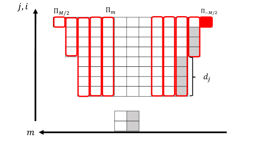
Figure 5: (color online) Definition of $\Pi_{m}$ where we sum up all populations of $|j,m,i\rangle$ in the density matrix for a fixed $m$.

$$\Pi_{m}=\sum^{M/2}_{j=|m|}\sum^{d_{j}}_{i=1}p_{j,m},$$ (30)

which is the total probability of the $m$-th column states, see Fig. 5. These states have the same energy. If $p_{j,m}=P_{m}$ (after Step II and the initial state), this is given as

$$\Pi_{m}={}_{M}C_{m+\frac{M}{2}}P_{m}.$$ (31)

We, now, consider the update rule of $\Pi_{m}$ under Step I and II. Let us denote the total probability of the $m$-th column states after the $n$ repetition by $\Pi^{(n)}_{m}$. The update rule depends on the sign of $m$.

First, we consider the case of positive $m$. These columns have no dark state, as shown in Fig. 6. According to the update rule (21), all elements in the $m$-th column can give half of its probability $P_{m}$ to the right ones and get half of the probability from the left ones by Step I, as shown in Fig. 6. Thus the update rule is given as

$$\Pi^{(n)}_{M/2} =\Pi^{(n-1)}_{M/2}/2,$$ (32)

$$\Pi^{(n)}_{m} =\Pi^{(n-1)}_{m}/2+\Pi^{(n-1)}_{m+1}/2,~{}~{}{\rm for}~{}~{}m>0,~{}m\neq M/2.$$

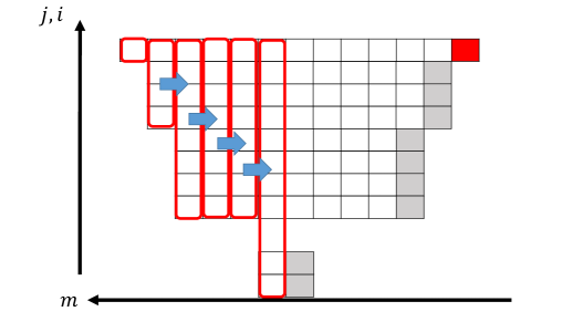
Figure 6: (color online) Update rule for $m>0$. Half of the population of $|j,m,i\rangle$ is transferred to that of $|j,m-1,i\rangle$.

Second, we consider the case for $m\leq 0$ where we have $d_{|m|}$ dark states (see Fig. 7). Then, only $({}_{M}C_{m+\frac{M}{2}}-d_{|m|})$ elements can give the half of its probability $P_{m}$ to the right ones. Because each element in the $m$-th column have the same probability $P_{m}$ due to Step II, we only have to count how many dark states in the $m$-th column in order to derive the update rule. A ratio between the number of the dark states and that of the total elements for a fixed $m$ determines the amount of the population to be transferred from the $m$-th column to the $(m+1)$-th column (see Fig. 7). Thus, the update rule for the $m\leq 0$ case is given as

$$\Pi^{(n)}_{m} =\frac{1}{2}\Bigl{(}1+\frac{d_{|m|}}{{}_{M}C_{m+\frac{M}{2}}}\Bigr{)}\Pi^{(n-1)}_{m}$$

$$+\frac{1}{2}\Bigl{(}1-\frac{d_{|m+1|}}{{}_{M}C_{1+m+\frac{M}{2}}}\Bigr{)}\Pi^{(n-1)}_{1+m},$$

$$~{}~{}~{}~{}~{}~{}~{}~{}~{}~{}{\rm for}~{}~{}m\leq 0,~{}m\neq-M/2,$$

$$\Pi^{(n)}_{-M/2} =\Pi^{(n-1)}_{-M/2}+\frac{1}{2}\Bigl{(}1-\frac{d_{|1-M/2|}}{{}_{M}C_{1}}\Bigr{)}\Pi^{(n-1)}_{1-M/2}.$$ (33)

The probability of each element $p_{j,m}$ in the $m$-th column can have different values after Step I because the rows labeled by $(j,i)$ are not equivalent. For instance, the probabilities of dark states will be relatively large comparing with those of the other states, see Fig. 7. If the probabilities $p_{j,m}$ depends on $j$, the above update rule does not work because this rule is derived under the assumption that $p_{j,m}=P_{m}$. Thus, when we repeat only Step I, the variable $\Pi_{m}$ is not appropriate to describe our process and we should use the original update rule (21) for $p_{j,m}$. On the other hand, when we insert Step II, since this step averages these probabilities, this update rule for $\Pi_{m}$ can be applied for the next repetition of Step I.

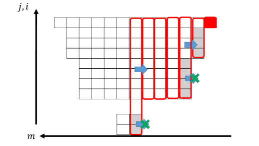
Figure 7: (color online) Update rule for $m\leq 0$. Half of the population of $|j,m,i\rangle$ is transferred to that of $|j,m-1,i\rangle$ unless $|j,m,i\rangle$ is a dark state that cannot transfer its population by the Step I.

Let us summarize the combined process of Step I and II. Note that the state after $n$ times repetition is given as

$$\rho^{(n)} =\sum^{M/2}_{m=-M/2}P^{(n)}_{m}\sum^{M/2}_{j=|m|}\sum^{d_{j}}_{i=1}|a_{j,m,i}\rangle\langle a_{j,m,i}|,$$ (34)

which is justified with the calculation above. By introducing the probability of the $m$-th column after $n$ times repetition like Eq. (30),

$$\Pi^{(n)}_{m}=\sum^{M/2}_{j=|m|}\sum^{d_{j}}_{i=1}P^{(n)}_{m}={}_{M}C_{m+\frac{M}{2}}P^{(n)}_{m},$$

the update rule is summarized as

$$\Pi^{(n+1)}_{M/2} =\Pi^{(n)}_{M/2}/2,$$

$$\Pi^{(n+1)}_{m} =\Pi^{(n)}_{m}/2+\Pi^{(n)}_{m+1}/2,~{}~{}{\rm for}~{}~{}m>0,~{}m\neq M/2,$$

$$\Pi^{(n+1)}_{m} =\frac{1}{2}\Bigl{(}1+\frac{d_{|m|}}{{}_{M}C_{m+\frac{M}{2}}}\Bigr{)}\Pi^{(n)}_{m}$$

$$+\frac{1}{2}\Bigl{(}1-\frac{d_{|m+1|}}{{}_{M}C_{1+m+\frac{M}{2}}}\Bigr{)}\Pi^{(n)}_{1+m},$$

$$~{}~{}~{}~{}~{}~{}~{}~{}~{}~{}~{}~{}{\rm for}~{}~{}m\leq 0,~{}m\neq-M/2,$$

$$\Pi^{(n+1)}_{-M/2} =\Pi^{(n)}_{-M/2}+\frac{1}{2}\Bigl{(}1-\frac{d_{|1-M/2|}}{{}_{M}C_{1}}\Bigr{)}\Pi^{(n)}_{1-M/2}.$$ (35)

As discussed previously, this update rule is based on the fact that $P^{(n)}_{m}$ is independent of $i$ and $j$ thanks to Step II. By using above $\Pi^{(n)}_{m}$, the density matrix after $n$-times repetition is given by

$$\rho^{(n)} =\sum^{M/2}_{m=-M/2}\frac{\Pi^{(n)}_{m}}{{}_{M}C_{m+\frac{M}{2}}}\sum^{M/2}_{j=|m|}\sum^{d_{j}}_{i=1}|a_{j,m,i}\rangle\langle a_{j,m,i}|.$$ (36)

Let us consider a probability of an excited state of the $k$-th spin,

$$p_{\uparrow,k}=\frac{1}{2}\bigl{(}1+{\rm Tr}(\sigma^{(k)}_{z}\rho)\bigr{)}.$$ (37)

Note that all spins are now equivalent. In this case, $p_{\uparrow,k}$ has no dependency on $k$, and thus we drop the index $k$ in this section. The dynamics of $p_{\uparrow}$ is summarized in Fig. 8 when $M=10,50,100$ and $200$. The $x$-axis is the number of steps divided by $M$. Since we assume that we wait until the system saturates at each Step I and II, the plot is independent of the interaction strength $g$ in Eq. (7) and the dephasing rate of the spins $\gamma^{\prime}$ in Eq. (10). When we perform only Step I, the population will be trapped by the dark states, and the final population of the excited state of the spins increases as $M$ does. On the other hand, the excited-state population converges to zero when we perform both Step I and II, as expected. Also, the plot of Step I+II shows a universal dynamics and does not depend on $M$.

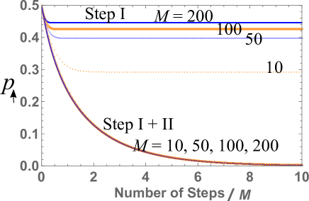
Figure 8: (color online) Plot of the excited-state population, $p_{\uparrow}$, of the qubit against the normalized number of steps. When we adopt only Step I, $p_{\uparrow}$ converges to finite non-zero values. On the other hand, when we adopt the Step I and II, $p_{\uparrow}$ approaches to zero, and the plots behave same regardless of the number of qubits. Here, we take $M=10,50,100$ and 200 from the bottom to top where $M$ denotes the number of qubits.

III Spin polarization with a flux qubit

We analyze a realistic polarization dynamics of electron spins based on the discussion in § II and show numerical simulations in various conditions. We consider the $0$th qubit as the flux qubit (FQ), which is highly controllable, and and consider the other qubits as the electron spins.

III.1 Parameters

We simulate the polarization dynamics with realistic parameters according to the Hamiltonian (2) and Lindbladian (II.1). The configuration of the FQ is assumed to be a $2r_{0}\times 2r_{0}$ square (see Fig. 9) and the parameters for numerical simulations are summarized in Table 1. Since fast reset of the superconducting qubit has been demonstrated with a resetting time of $120$ ns where the the longitudinal relaxation time $T_{1}$ of the qubit can be controlled over a factor of $50$ [36, 37], we assume that the time required for initialization is $t_{\rm i}=5\times 10^{-6}$ s.

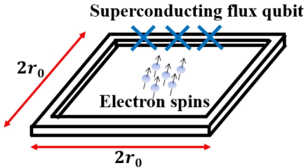
Figure 9: (color online) Illustration of our system composed of the superconducting flux qubit (FQ) and electron spins. The FQ consists in a square loop containing three Josephson junctions, illustrated as three blue $\times$’s. The electron spins are located in the middle of the FQ, and they are inductively coupled with the FQ.

The electron spins are located in the middle of a square determined by the FQ (see Fig. 9). Their interaction strengths $g_{k}$’s with the FQ during the spin lock are given as [38, 39, 31]

$$g_{k} =\frac{\varepsilon}{\sqrt{\varepsilon^{2}+\Delta^{2}}}\frac{\gamma_{e}\mu_{0}I_{p}}{2\pi}\sum_{i=1}^{4}\frac{1}{r_{i}^{(k)}},$$ (38)

where $r_{i}^{(k)}$, $\gamma_{e}$, $\mu_{0}$ are the distance from $i$-th side of the FQ to an $k$-th spin, the gyromagnetic ratio of an electron spin, and the Vacuum permeability, respectively. If the electron spin is placed in the middle of a FQ, we obtain $g_{k}=g_{0}=175$ rad/s with the parameters given in Table 1. This value gives the energy scale of the interaction between the FQ and spins.

parameter of FQ	symbol	value
size	$r_{0}$	$3.0\times 10^{-6}$ m
persistent current	$I_{p}$	180 nA
longitudinal relaxation time	$T_{1}^{\rm(FQ)}$	$200\times 10^{-6}$ s
transversal relaxation time	$T_{2}^{\rm(FQ)}$	$30\times 10^{-6}$ s
energy gap	$\Delta/2\pi$	$5.37\times 10^{9}$ Hz
detuning parameter	$\varepsilon/2\pi$	$0.112\times 10^{9}$ Hz
time required for initialization	$t_{\rm i}$	$5\times 10^{-6}$ s
interval between initialization	$t_{\rm int}$	$95\times 10^{-6}$ s

Table 1: Parameters of the FQ for numerical simulations [40, 23].

We also assume that the longitudinal relaxation time $T_{1}^{(e)}=1.0$ s and the transversal relaxation time $T_{2}^{(e)}=1.0\times 10^{-3}$ s for electron spins [41, 42, 43].

III.2 Simulations

We numerically calculate the system dynamics according to the operator sum formalism [44, 45, 46]. The density matrix $\rho$ is updated as follows.

$$\rho(t)\rightarrow\rho^{\prime}=e^{-i{\cal H}\delta}\rho\,e^{i{\cal H}\delta}\rightarrow\rho(t+\delta)=\rho^{\prime}+{\cal L}[\rho^{\prime}]\delta,$$ (39)

where we take $\delta=5\times 10^{-6}$ s which is small enough compared with the characteristic time scale such as $T_{1},T_{2}$ of the FQ or spins, and $1/g_{k}$. We let the system evolve by this formalism for a time $t_{\rm int}$. We consider various ${\cal H}$’s and ${\cal L}$’s by changing parameters in § III.2 1 $\sim$ 4.

The initial state of the electron spin is a completely mixed state. We assume that the FQ is periodically initialized into the ground state at $t_{n}=(n-1)(t_{\rm i}+t_{\rm int}$) where $n$ denotes natural numbers. We define this period as a single step. Since the initialization of the FQ can be much faster than the time scale of the decay of the electron spins, we assume that the state of the electron spins does not change during the initialization of the FQ.

In the numerical calculations, we do not separate the dynamics into Step I and Step II. By applying both the dephasing of the electron spins and the interaction between the FQ and the electron spins, we simultaneously perform Step I and Step II.

III.2.1 $\omega_{k}^{\prime}=0$, $g_{k}=g_{0}$, and $\gamma_{\rm T}^{\rm(l)}=\gamma_{\rm L}^{\rm(l)}=0$ case

We first simulate the case when there is no decoherence in order to illustrate the influence of dark states on the polarization process. We assume that ${\omega_{k}}^{\prime}=0$ and $g_{k=1\sim M}=g_{0}$ in Eq. (2) and $\gamma_{\rm T}^{\rm(l=0\sim M)}=\gamma_{\rm L}^{\rm(l=0\sim M)}=0$ in Eq. (II.1). Figure 10 shows the dynamics of $p_{\uparrow}$. Note that all spins are equivalent and thus $p_{\uparrow,k}$’s are identical. Because of the dark states, $p_{\uparrow}$ saturates in the large step limit. Note also that the cooling rate in this simulation is much slower than that shown in Fig. 8. This is because, in Fig. 10, the interaction time $t_{\rm{int}}$ is much smaller than $1/g_{k}$, and the population transfer between the electron spins and the FQ is small at a single step. On the other hand, in Fig. 8, half of the ground-state population is transferred to the electron spins at a single step.

Figure 10: (color online) Plot of the excited-state population, $p_{\uparrow}$, of the spins against the number of steps for $M=1\sim 9$ of electron spins. The initial state of the spins is the completely mixed state. We set the parameters as $\omega_{k=1\sim M}^{\prime}=0$, $g_{k=1\sim M}=g_{0}$, and $\gamma_{\rm T}^{\rm(l=0\sim M)}=\gamma_{\rm L}^{\rm(l=0\sim M)}=0$.

III.2.2 $\omega_{k}^{\prime}=0$ and $\gamma_{\rm T}^{\rm(l)}=\gamma_{\rm L}^{\rm(l)}=0$ case

We consider the case when $g_{k}$ is inhomogeneous because of random spin positioning on a substrate according to Eq. (38).

Figure 11 shows $p_{\uparrow,k}$ when $M=7$. Due to the different values of $g_{k}$ (see the caption of Fig. 11), $p_{\uparrow,k}$ approaches a different saturation value and does not approach zero.

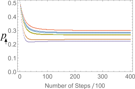
Figure 11: (color online) Plot of the excited-state population, $p_{\uparrow,k}$, of the spins against the number of steps for $M=7$ when $\omega_{k=1\sim M}^{\prime}=0$, $\{g_{k=1\sim M}\}=\{151,221,173,204,197,176,180\}$ rad/s, $\gamma_{\rm T}^{\rm(l=0\sim M)}=\gamma_{\rm L}^{\rm(l=0\sim M)}=0$. The different lines correspond to $g_{k}$.

III.2.3 $\omega_{k}^{\prime}=0,\gamma_{\rm T}^{\rm(l)}\neq 0$, and $\gamma_{\rm L}^{\rm(l)}=0$ case

We consider the case when $g_{k}$ is inhomogeneous with a finite dephasing rate of $\gamma_{\rm T}^{\rm(l=0\sim M)}\neq 0$. Figure 12 shows the case with $M=7$. Due to the dephasing on spins, $p_{\uparrow,k}$ approaches zero with different cooling rate according to $g_{k}$. This observation with Fig. 11 shows that the dephasing leads $p_{\uparrow,k}=0$ at the large step limit.

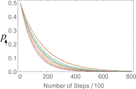
Figure 12: (color online) Plot of the excited-state population, $p_{\uparrow,k}$, of the electron spins against the number of steps for $M=7$ when $\omega_{k=1\sim M}^{\prime}=0$, $\{g_{k=1\sim M}\}=\{179,202,194,161,178,204,156\}$ rad/s, $\gamma_{\rm L}^{\rm(l=0\sim M)}=0$, $\gamma_{\rm T}^{(0)}=1/T_{2}^{\rm(FQ)}$, and $\gamma_{\rm T}^{(k=1\sim M)}=1/T_{2}^{(e)}$.

III.2.4 realistic case

To support our simplified model discussed in § II, we have considered non-realistic cases in § III.2 $1\sim 3$ where some imperfections have been ignored. We will, here, discuss a realistic case when both $\omega_{k}^{\prime}$ and $g_{k}$ are inhomogeneous with finite decay rates of $\gamma_{\rm T}^{\rm(l)}\neq 0$ and $\gamma_{\rm L}^{\rm(l)}\neq 0$.

We show the case for $M=7$ in Fig. 13. $p_{\uparrow,k}$ approaches 0.16 regardless of $\omega_{k}^{\prime}$ and $g_{k}$. It converges to non-zero values because of $\gamma_{\rm L}^{(k)}\neq 0$. Due to a thermal relaxation process, the state of the electron spins will be a Gibbs state in a natural environment, and its excited-state population is $p_{\uparrow}=0.47$ at 1 mT and 10 mK (a typical operation temperature of a FQ) environment. This means that our cooling scheme with the FQ is especially useful when we perform an ESR with the FQ: A sensitivity of ESR measurements is proportional to $p_{\downarrow}-p_{\uparrow}$ [14, 47], and so the sensitivity of ESR with our polarization scheme leads 10 times better than the conventional one without active cooling. Also, it is worth mentioning that the actual temperature of the electron spins in the dilution refrigerator might be 50 mK or more and not 10 mK [7, 8] because $T_{1}$ of the electron spins is large [20]. Moreover, an interval between measurements in the standard ESR should be a few time larger than $T_{1}$ of the electron spins. Therefore, as $T_{1}$ becomes longer, our approach does more efficient than the conventional one.

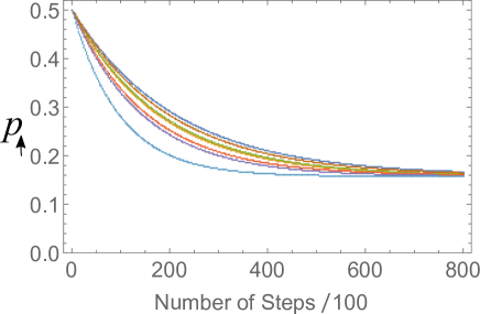
Figure 13: (color online) Realistic simulations. We plot the excited-state population, $p_{\uparrow,k}$, of the electron spins against the number of steps for $M=7$ when $\omega_{k=1\sim M}^{\prime}=\{4736,455,-6867,1773,-1569,703,-5204\}$ rad/s, $\{g_{k=1\sim M}\}=\{193,163,175,225,178,160,268\}$ rad/s, $\gamma_{\rm L}^{(0)}=1/T_{1}^{\rm(FQ)}$, $\gamma_{\rm L}^{({k=1\sim M})}=1/T_{1}^{(e)}$, $\gamma_{\rm T}^{(0)}=1/T_{2}^{\rm(FQ)}$, and $\gamma_{\rm T}^{({k=1\sim M})}=1/T_{2}^{(e)}$.

IV Conclusion

In conclusion, we propose a scheme to polarize electron spins with a superconducting flux qubit (FQ). Since we cannot apply large magnetic fields for the FQ to work, there is a large energy gap between the electron spins and FQ. To achieve a strong interaction between them, we adopt a spin-lock technique for the FQ. A Rabi frequency of the FQ can be as small as resonance frequencies of the electron spins and thus the efficient energy transfer between them can occur. We find that homogeneous electron spins without any decoherence cannot be cooled down to the ground state with the FQ, because the electron spins in dark states cannot be coupled to the FQ. Interestingly, dephasing on the electron spins (usually they are not avoidable in experiments) allows them to escape from the dark states. We show that the electron spins can be polarized in realistic conditions by using our scheme.

Appendix

IV.1 Proof of Eq. (26)

We, first, prove

$$P\rho_{j,m}P^{\dagger}=\rho_{j,m}$$ (40)

for any permutation matrix $P$. Note that any permutation matrix $P$ satisfies

$$[P,S_{z}]=0,\,\,[P,S^{2}]=0,$$ (41)

where $S^{2}=S_{x}^{2}+S_{y}^{2}+S_{z}^{2}$. This is directly proved by the permutation invariance $PS_{z}P^{\dagger}=S_{z}$ and $PS^{2}P^{\dagger}=S^{2}$ in the following way:

$$PS_{z}=PS_{z}P^{\dagger}P=S_{z}P,$$

$$PS^{2}=PS^{2}P^{\dagger}P=S^{2}P,$$ (42)

where we use $P^{-1}=P^{\dagger}$.

Let us write the action of $P$ on $|j,m,i\rangle$ as

$$P|j,m,i\rangle=\sum_{j^{\prime},m^{\prime},i^{\prime}}P^{j,m,i}_{j^{\prime},m^{\prime},i^{\prime}}|j^{\prime},m^{\prime},i^{\prime}\rangle.$$ (43)

We consider the explicit form of $P^{j,m,i}_{j^{\prime},m^{\prime},i^{\prime}}$. By considering the following fact,

$$0= [P,S_{z}]|j,m,i\rangle=PS_{z}|j,m,i\rangle-S_{z}P|j,m,i\rangle$$

$$= mP|j,m,i\rangle-S_{z}\sum_{j^{\prime},m^{\prime},i^{\prime}}P^{j,m,i}_{j^{\prime},m^{\prime},i^{\prime}}|j^{\prime},m^{\prime},i^{\prime}\rangle$$

$$= mP|j,m,i\rangle-\sum_{j^{\prime},m^{\prime},i^{\prime}}m^{\prime}P^{j,m,i}_{j^{\prime},m^{\prime},i^{\prime}}|j^{\prime},m^{\prime},i^{\prime}\rangle$$

$$= \sum_{j^{\prime},m^{\prime},i^{\prime}}(m-m^{\prime})P^{j,m,i}_{j^{\prime},m^{\prime},i^{\prime}}|j^{\prime},m^{\prime},i^{\prime}\rangle.$$ (44)

This implies that $P^{j,m,i}_{j^{\prime},m^{\prime},i^{\prime}}$ has the form of $\delta^{m}_{m^{\prime}}\tilde{P}^{j,i}_{j^{\prime},i^{\prime}}$. By using the commutation relation about $S^{2}$, we can prove that $P^{j,m,i}_{j^{\prime},m^{\prime},i^{\prime}}$ has the form of $\delta^{m}_{m^{\prime}}\delta^{j}_{j^{\prime}}\tilde{\tilde{P}}^{i}_{i^{\prime}}$ in the same manner as above. Thus, $P$ is a block-diagonal matrix with respect to the basis $\{|j,m,i\rangle\}_{j,m,i}$. The explicit form of $P$ is given as

$$P=\sum_{j,m,i,i^{\prime}}\tilde{\tilde{P}}^{i}_{i^{\prime}}|j,m,i\rangle\langle j,m,i^{\prime}|.$$ (45)

because $P$ is a unitary matrix, $\tilde{\tilde{P}}^{i^{\prime}}_{i}$ is also unitary, i.e., $\sum_{i^{\prime\prime}}\tilde{\tilde{P}}^{i}_{i^{\prime\prime}}\left(\tilde{\tilde{P}}^{i^{\prime}}_{i^{\prime\prime}}\right)^{*}=\delta_{i,i^{\prime}}$. Then we can explicitly show,

$$P\rho_{j,m}P^{\dagger}$$

$$=\sum_{j_{1,2},m_{1,2},i_{1,2,3,4}}\tilde{\tilde{P}}^{i_{1}}_{i_{2}}|j_{1},m_{1},i_{1}\rangle\langle j_{1},m_{1},i_{2}|$$

$$\quad\quad\rho_{j,m}\left(\tilde{\tilde{P}}^{i_{4}}_{i_{3}}\right)^{*}|j_{2},m_{2},i_{3}\rangle\langle j_{2},m_{2},i_{4}|$$

$$=\sum_{i,i_{1},i_{4}}\tilde{\tilde{P}}^{i_{1}}_{i}\left(\tilde{\tilde{P}}^{i_{4}}_{i}\right)^{*}|j,m,i_{1}\rangle\langle j,m,i_{4}|$$

$$=\sum_{i}|j,m,i\rangle\langle j,m,i|=\rho_{j,m}.$$ (46)

We now proved Eq. (40), which means that all the diagonal elements of $\rho_{j,m}$ represented in the binary basis ($|\underbrace{11\cdots 1}_{n/2+m}\underbrace{00\cdots 0}_{n/2-m}\rangle$ and all its permutations) is identical, that is,

$$\rho_{j,m}=\frac{d_{j}}{{}_{M}C_{m+\frac{M}{2}}}|0\rangle\langle 0|\otimes\begin{pmatrix}1&.&.&\ldots&.\\ .&1&.&\ldots&.\\ .&.&1&\ldots&.\\ \vdots&\vdots&\vdots&\ddots&\vdots\\ .&.&.&\ldots&1\\ \end{pmatrix}.$$ (47)

This matrix is a ${}_{M}C_{m+\frac{M}{2}}\times{}_{M}C_{m+\frac{M}{2}}$ matrix while its matrix rank is $d_{j}$. The effect of independent dephasing ${\cal E}_{\rm II}$ makes the non-diagonal elements of this matrix be $0$. Thus, after Step II, the density matrix $\rho_{j,m}$ becomes ${\cal E}_{\rm II}(\rho_{j,m})$ given as

$${\cal E}_{\rm II}(\rho_{j,m})=\frac{d_{j}}{{}_{M}C_{m+\frac{M}{2}}}|0\rangle\langle 0|\otimes\begin{pmatrix}1&0&0&\ldots&0\\ 0&1&0&\ldots&0\\ 0&0&1&\ldots&0\\ \vdots&\vdots&\vdots&\ddots&\vdots\\ 0&0&0&\ldots&1\\ \end{pmatrix},$$ (48)

which is the identity matrix of the space spanned by the binary basis with fixed $m$. Although the above matrix is represented in the binary basis, because the identity matrix is invariant under any unitary transformation on this space, Eq. (48) can be rewritten as

$${\cal E}_{\rm II}(\rho_{j,m})=\frac{d_{j}}{{}_{M}C_{m+\frac{M}{2}}}|0\rangle\langle 0|\otimes\sum^{M/2}_{s=|m|}\sum^{d_{s}}_{i=1}|s,m,i\rangle\langle s,m,i|.$$ (49)

Thus, Eq. (26) is proved.

References

- Kubo et al. [2012] Y. Kubo, I. Diniz, C. Grezes, T. Umeda, J. Isoya, H. Sumiya, T. Yamamoto, H. Abe, S. Onoda, T. Ohshima, et al., Physical Review B 86, 064514 (2012).
- Toida et al. [2016] H. Toida, Y. Matsuzaki, K. Kakuyanagi, X. Zhu, W. J. Munro, K. Nemoto, H. Yamaguchi, and S. Saito, Applied Physics Letters 108, 052601 (2016).
- Bienfait et al. [2016a] A. Bienfait, J. Pla, Y. Kubo, M. Stern, X. Zhou, C. Lo, C. Weis, T. Schenkel, M. Thewalt, D. Vion, et al., Nature nanotechnology 11, 253 (2016a).
- Eichler et al. [2017] C. Eichler, A. Sigillito, S. A. Lyon, and J. R. Petta, Physical review letters 118, 037701 (2017).
- Probst et al. [2017] S. Probst, A. Bienfait, P. Campagne-Ibarcq, J. Pla, B. Albanese, J. Da Silva Barbosa, T. Schenkel, D. Vion, D. Esteve, K. Mølmer, et al., Applied Physics Letters 111, 202604 (2017).
- Bienfait et al. [2017] A. Bienfait, P. Campagne-Ibarcq, A. Kiilerich, X. Zhou, S. Probst, J. Pla, T. Schenkel, D. Vion, D. Esteve, J. Morton, et al., Physical Review X 7, 041011 (2017).
- Budoyo et al. [2018a] R. P. Budoyo, K. Kakuyanagi, H. Toida, Y. Matsuzaki, W. J. Munro, H. Yamaguchi, and S. Saito, Physical Review Materials 2, 011403 (2018a).
- Toida et al. [2019] H. Toida, Y. Matsuzaki, K. Kakuyanagi, X. Zhu, W. J. Munro, H. Yamaguchi, and S. Saito, Communications Physics 2, 1 (2019).
- Ranjan et al. [2020] V. Ranjan, S. Probst, B. Albanese, T. Schenkel, D. Vion, D. Esteve, J. Morton, and P. Bertet, Applied Physics Letters 116, 184002 (2020).
- Wiemann et al. [2015] Y. Wiemann, J. Simmendinger, C. Clauss, L. Bogani, D. Bothner, D. Koelle, R. Kleiner, M. Dressel, and M. Scheffler, Applied Physics Letters 106, 193505 (2015).
- Chen et al. [2018] Y.-H. Chen, X. Fernandez-Gonzalvo, S. P. Horvath, J. V. Rakonjac, and J. J. Longdell, Physical Review B 97, 024419 (2018).
- Yue et al. [2017] G. Yue, L. Chen, J. Barreda, V. Bevara, L. Hu, L. Wu, Z. Wang, P. Andrei, S. Bertaina, and I. Chiorescu, Applied Physics Letters 111, 202601 (2017).
- Budoyo et al. [2020] R. P. Budoyo, K. Kakuyanagi, H. Toida, Y. Matsuzaki, and S. Saito, Applied Physics Letters 116, 194001 (2020).
- Wertz [2012] J. Wertz, Electron spin resonance: elementary theory and practical applications (Springer Science & Business Media, 2012).
- Purcell [1995] E. M. Purcell, in Confined Electrons and Photons (Springer, 1995) pp. 839–839.
- Bienfait et al. [2016b] A. Bienfait, J. Pla, Y. Kubo, X. Zhou, M. Stern, C. Lo, C. Weis, T. Schenkel, D. Vion, D. Esteve, et al., Nature 531, 74 (2016b).
- Amsüss et al. [2011] R. Amsüss, C. Koller, T. Nöbauer, S. Putz, S. Rotter, K. Sandner, S. Schneider, M. Schramböck, G. Steinhauser, H. Ritsch, J. Schmiedmayer, and J. Majer, Phys. Rev. Lett. 107, 060502 (2011).
- Probst et al. [2013] S. Probst, H. Rotzinger, S. Wünsch, P. Jung, M. Jerger, M. Siegel, A. V. Ustinov, and P. A. Bushev, Phys. Rev. Lett. 110, 157001 (2013).
- Angerer et al. [2017] A. Angerer, S. Putz, D. O. Krimer, T. Astner, M. Zens, R. Glattauer, K. Streltsov, W. J. Munro, K. Nemoto, S. Rotter, J. Schmiedmayer, and J. Majer, Science Advances 3, 10.1126/sciadv.1701626 (2017).
- Budoyo et al. [2018b] R. P. Budoyo, K. Kakuyanagi, H. Toida, Y. Matsuzaki, W. J. Munro, H. Yamaguchi, and S. Saito, Applied Physics Express 11, 043002 (2018b).
- Hartmann and Hahn [1962] S. Hartmann and E. Hahn, Physical Review 128, 2042 (1962).
- You et al. [2007] J. You, X. Hu, S. Ashhab, and F. Nori, Physical Review B 75, 140515 (2007).
- Yan et al. [2016] F. Yan, S. Gustavsson, A. Kamal, J. Birenbaum, A. P. Sears, D. Hover, T. J. Gudmundsen, D. Rosenberg, G. Samach, S. Weber, et al., Nature communications 7, 1 (2016).
- Abdurakhimov et al. [2019] L. V. Abdurakhimov, I. Mahboob, H. Toida, K. Kakuyanagi, and S. Saito, Applied Physics Letters 115, 262601 (2019).
- Laraoui and Meriles [2013] A. Laraoui and C. A. Meriles, ACS nano 7, 3403 (2013).
- Scheuer et al. [2016] J. Scheuer, I. Schwartz, Q. Chen, D. Schulze-Sünninghausen, P. Carl, P. Höfer, A. Retzker, H. Sumiya, J. Isoya, B. Luy, et al., New journal of Physics 18, 013040 (2016).
- Ping et al. [2002] J. Ping, F. Wang, and J.-q. Chen, Group representation theory for physicists (World Scientific Publishing Company, 2002).
- Boller et al. [1991] K.-J. Boller, A. Imamoğlu, and S. E. Harris, Physical Review Letters 66, 2593 (1991).
- Fleischhauer et al. [2005] M. Fleischhauer, A. Imamoglu, and J. P. Marangos, Reviews of modern physics 77, 633 (2005).
- Zhu et al. [2014] X. Zhu, Y. Matsuzaki, R. Amsüss, K. Kakuyanagi, T. Shimo-Oka, N. Mizuochi, K. Nemoto, K. Semba, W. J. Munro, and S. Saito, Nature communications 5, 1 (2014).
- Matsuzaki et al. [2015a] Y. Matsuzaki, X. Zhu, K. Kakuyanagi, H. Toida, T. Shimo-Oka, N. Mizuochi, K. Nemoto, K. Semba, W. J. Munro, H. Yamaguchi, et al., Physical review letters 114, 120501 (2015a).
- Matsuzaki et al. [2015b] Y. Matsuzaki, X. Zhu, K. Kakuyanagi, H. Toida, T. Shimooka, N. Mizuochi, K. Nemoto, K. Semba, W. Munro, H. Yamaguchi, et al., Physical Review A 91, 042329 (2015b).
- Putz et al. [2017] S. Putz, A. Angerer, D. O. Krimer, R. Glattauer, W. J. Munro, S. Rotter, J. Schmiedmayer, and J. Majer, Nature Photonics 11, 36 (2017).
- Julsgaard et al. [2013] B. Julsgaard, C. Grezes, P. Bertet, and K. Mølmer, Phys. Rev. Lett. 110, 250503 (2013).
- Probst et al. [2015] S. Probst, H. Rotzinger, A. Ustinov, and P. Bushev, Physical Review B 92, 014421 (2015).
- Reed et al. [2010] M. D. Reed, B. R. Johnson, A. A. Houck, L. DiCarlo, J. M. Chow, D. I. Schuster, L. Frunzio, and R. J. Schoelkopf, Applied Physics Letters 96, 203110 (2010).
- Hsu et al. [2020] H. Hsu, M. Silveri, A. Gunyhó, J. Goetz, G. Catelani, and M. Möttönen, Phys. Rev. B 101, 235422 (2020).
- Marcos et al. [2010] D. Marcos, M. Wubs, J. Taylor, R. Aguado, M. D. Lukin, and A. S. Sørensen, Physical review letters 105, 210501 (2010).
- Twamley and Barrett [2010] J. Twamley and S. D. Barrett, Physical Review B 81, 241202 (2010).
- Bylander et al. [2011] J. Bylander, S. Gustavsson, F. Yan, F. Yoshihara, K. Harrabi, G. Fitch, D. G. Cory, Y. Nakamura, J. S. Tsai, and W. D. Oliver, Nat. Phys. 7, 565 (2011).
- Tyryshkin et al. [2012] A. M. Tyryshkin, S. Tojo, J. J. Morton, H. Riemann, N. V. Abrosimov, P. Becker, H.-J. Pohl, T. Schenkel, M. L. Thewalt, K. M. Itoh, et al., Nature materials 11, 143 (2012).
- Herbschleb et al. [2019] E. Herbschleb, H. Kato, Y. Maruyama, T. Danjo, T. Makino, S. Yamasaki, I. Ohki, K. Hayashi, H. Morishita, M. Fujiwara, et al., Nature communications 10, 1 (2019).
- Amsüss et al. [2011] R. Amsüss, C. Koller, T. Nöbauer, S. Putz, S. Rotter, K. Sandner, S. Schneider, M. Schramböck, G. Steinhauser, H. Ritsch, et al., Physical review letters 107, 060502 (2011).
- Zanardi [1998] P. Zanardi, Physical Review A 57, 3276 (1998).
- Kondo et al. [2016] Y. Kondo, Y. Matsuzaki, K. Matsushima, and J. G. Filgueiras, New Journal of Physics 18, 013033 (2016).
- Bando et al. [2020] M. Bando, T. Ichikawa, Y. Kondo, N. Nemoto, M. Nakahara, and Y. Shikano, Scientific reports 10, 1 (2020).
- Miyanishi et al. [2020] K. Miyanishi, Y. Matsuzaki, H. Toida, K. Kakuyanagi, M. Negoro, M. Kitagawa, and S. Saito, Physical Review A 101, 052303 (2020).