Implicit Solvation Methods
for Catalysis at Electrified Interfaces

Abstract

Implicit solvation is an effective, highly coarse-grained approach in atomic-scale simulations to account for a surrounding liquid electrolyte on the level of a continuous polarizable medium. Originating in molecular chemistry with finite solutes, implicit solvation techniques are now increasingly used in the context of first-principles modeling of electrochemistry and electrocatalysis at extended (often metallic) electrodes. The prevalent ansatz to model the latter electrodes and the reactive surface chemistry at them through slabs in periodic boundary condition supercells brings its specific challenges. Foremost this concerns the diffculty to describe the entire double layer forming at the electrified solid-liquid interface (SLI) within supercell sizes tractable by commonly employed density-functional theory (DFT). We review liquid solvation methodology from this specific application angle, highlighting in particular its use in the widespread ab initio thermodynamics approach to surface catalysis. Notably, implicit solvation can be employed to mimic a polarization of the electrode’s electronic density under the applied potential and the concomitant capacitive charging of the entire double layer beyond the limitations of the employed DFT supercell. Most critical for continuing advances of this effective methodology for the SLI context is the lack of pertinent (experimental or high-level theoretical) reference data needed for parametrization.

1 Introduction

Electrocatalysis, i.e. potential-driven chemistry at electrified interfaces, is one of the pillars of a future sustainable energy landscape, providing a green storage of renewable energy and its conversion to valuable chemicals.^{1, 2, 3} The concomitant increased global interest in electrochemical processes at extended surfaces and interfaces has triggered unprecedented academic and industrial research efforts to optimize catalyst materials and electrochemical cell designs for maximal efficiency, sustainability, and durability. In this development, predictive-quality computational simulations have played a key role, augmenting experimental results with atomic-scale mechanistic insights and increasingly supporting catalyst discovery and optimization.^{4, 5, 6, 7, 8, 9}

Given the fact that electrochemical reactions depend on the movement of charges, the respective computer simulations are by necessity based on a quantum mechanical description of the involved materials. Yet, while first-principles quantum chemistry provides a conceptually exact toolkit to simulate chemical reactions, current (super-)computers can even with most efficient semi-local density-functional theory (DFT) only simulate a limited amount of atoms and at time scales where chemical reactions cannot be statistically resolved.¹⁰ Fortunately, energy conversion processes can often be considered as a path through thermodynamically equilibrated, meta-stable states, separated by kinetic barriers which are often in a direct, linear relation with free energy differences between those states.¹¹ Furthermore, chemical reactions frequently occur at defined locations, the so-called active sites, and have a quite localized impact on their surrounding.¹² As a consequence, and as shown in Fig. 1, to a good approximation one can in many cases carve out from the full constant-particle thermodynamic system a smaller grand-canonical sub-system which is in equilibrium with bulk reservoirs of species.¹³

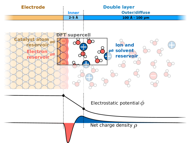
Figure 1: Ab initio thermodynamics approach to electrified solid-liquid interfaces as occurring in electrocatalysis. The electrode is here negatively charged and this surface charge is compensated by the built up of counter charge in the electrolyte. The formed electric double layer (DL) can be pictured as a localized capacitor at the interface of electrode and a rather rigid layer of ions (inner DL or Helmholtz layer) and a long-range contribution (outer or diffuse DL). As in particular the spatial extent of the diffuse DL challenges efficient first-principles calculations, the ab initio thermodynamics approach considers a grand-canonical ensemble in which a finite supercell computed e.g. with DFT is in equilibrium with appropriate reservoirs for the catalyst atoms, solvent species and electrons. Since the supercell does then generally not comprise the entire DL, it misses part of the compensating charge and does not necessarily have to be overall charge neutral.

In this ab initio thermodynamics approach to surface catalysis, this sub-system in form of a model of the active site and any adsorbed reaction intermediates can then conveniently be computed as a slab within a periodic boundary condition supercell, and a grand-canonical thermodynamic framework is used to connect the obtained first-principles energetics with the reservoirs through defined chemical potentials for the catalyst atoms and the reactants. In thermal heterogeneous catalysis,^{14, 15, 16, 17, 18, 19, 13} where this approach was pioneered and is widely used, the surrounding reactant environment and its corresponding reservoirs are generally well approximated by neutral ideal gases. Concomitantly, also the finite supercell is charge neutral and there is no necessity to explicitly include in the first-principles supercell calculation the gas-phase species that would in principle fill the finite volume between the periodically repeating slabs. Instead, the actual DFT calculations are simply performed for a slab in perfect vacuum. Unfortunately, the situation is significantly more complex in surface electrocatalysis,²⁰ where the solid catalyst exchanges electrons with the reactants and is in contact with a liquid electrolyte forming a solid-liquid interface (SLI). As further detailed below, this enforces the consideration of charged reservoirs (electrons, protons, or ionic species in the electrolyte) with which the then no longer necessarily overall charge-neutral supercell is in electrochemical equilibrium, cf. Fig. 1. Furthermore, this exchange of charge species with the respective reservoirs and potentially ongoing surface reactions are driven by applied electrostatic potentials, which directly interact with the solvent structure near the surface. Apart from the specifically adsorbed reaction intermediates there is thus now in principle also the need to describe the liquid electrolyte species within the finite volume between the periodically repeating slabs in the supercell.

It is from the objective of reducing this complexity and recovering the efficiency of ab initio thermodynamics as known from thermal surface catalysis, where much of the renewed interest in implicit solvation schemes in this field comes from.^{21, 22, 23, 24, 25, 26} Corresponding methodologies form in general a long-standing coarse-grained approach to describe a solvent environment on the level of a dielectric continuum. While they thus have their own history (in particular for molecular systems), their application to extended SLIs and the context of ab initio thermodynamics has its specific challenges and merits. It is from this particular angle that we here review such methodologies and discuss their recent application to the surface electrocatalysis context, especially at metal electrodes and for liquid, mostly aqueous electrolytes. We refer to excellent and comprehensive reviews for full theoretical and technical details and the more traditional uses of implicit solvation methods for molecular systems,^{27, 28, 29} and content ourselves here with a focused exposition of the general concepts. Instead, we elaborate more on the specific demands, benefits and persisting issues when applying such methods to electrified interfaces.

To set the stage for such a discussion, Fig. 1 also summarizes some key properties and specificities of the electrified SLI. Central to this is the separation of (ionic and electronic) charges that results from the interaction of the metallic electrode with the surrounding electrolyte under an applied potential. A potential-dependent amount of net charge $\rho$ is thus localized on the electrode surface and counter charges in the form of dissolved ions are redistributed to a certain depth into the electrolyte to compensate for this net charge. Additionally, rotational, translational and even vibrational degrees of freedom in particular of polar electrolyte molecules (like water in aqueous electrolytes) will be affected within this formed, so-called electric double layer (DL).^{30, 31} As a consequence of the concomitant screening, the electrostatic potential $\phi$ drops over the width of the DL. At least in aqueous electrolytes, this drop generally occurs over two regions: the inner or Helmholtz³² layer (iDL), where $\phi$ drops linearly, and the outer or diffuse layer, where it drops non-linearly. The capacitance $C$ arising from the charging of the DL is correspondingly also commonly separated into an inner and an outer contribution.^{33, 34} While this was originally made without a direct reference to the actual atomic-scale nature of the DL, the different dielectric property of the iDL is now related to a crowding of counter ions directly at the charged electrode. This leads to the formation of a compact layer with almost rigid water molecules and thus a small dielectric permittivity.^{33, 35, 36, 31} In contrast, depending on the applied potential and electrolyte concentration, the more diffuse re-distribution of ions in the outer DL can extend over hundreds of Ångstroms into the electrolyte, cf. Fig. 1.

From this simplified capacitor picture, it becomes clear that the true amount of net surface charge on the electrode at a given applied potential is a sensitive function of the entire DL. Adsorption energies and therefore reaction pathways in turn often depend sensitively on this surface charge and the potential drop in the DL, e.g. via electrostatic interactions of dipolar adsorbates with the electric field.^{37, 38, 39, 40, 41} Already this aspect alone thus reveals that electrochemical activity in the SLI is generally not merely a function of the electrode aka catalyst material. Instead, it is equally influenced by the electrolyte and the concomitant DL. Additional aspects of this influence concern also more classic solvation effects like steric or bonding interactions with electrolyte species in the inner DL (in aqueous electrolytes e.g. prominently hydrogen bonds).^{42, 43, 44, 45, 46} Capturing these multifaceted influences and in particular their net effect on reaction energetics is correspondingly a pivotal ingredient of predictive-quality computational simulations and theoretical analyses of catalysis at electrified interfaces. At the same time and as further discussed in Section 2.1 below, the outer DL’s large extent plus the ions’ very slow, typically nanosecond time scale diffusion render any atomic-scale first-principles calculations including an explicit and dynamical account of the full DL still prohibitively expensive.⁴⁷

Implicit solvation schemes are at the opposite end and promise an unsurpassed computational efficiency in simulating the SLI.^{22, 25, 21} In their original molecular form, these schemes define a solvation cavity in which the solute is embedded and surrounded by a dielectric continuum representing the solvent’s dielectric response.^{48, 28} On top of that, the contribution of ions to the overall electrostatic response can be modeled. In the application to SLIs, such implicit solvation schemes thus foremost allow to appropriately describe the capacitive charging of the DL beyond the confines of the finite supercell—though requiring the integration into an ab initio thermodynamics framework to appropriately account for the flow of particles between the subsystem and the reservoirs (cf. Fig. 1) as detailed in Section 3.1. Next to effectively describing the counter charge, implicit solvation models obviously also aim to capture plain solvation effects.²⁸ Yet, with the solvent represented by a continuum this is, of course, only on a highly effective, parametrized level, in particular in the present state-of-the-art that also includes the inner DL into the implicit description.^{22, 25, 21} As further discussed in Section 2.6, this situation is aggravated even more by the scarcity of reliable experimental SLI data to fit the empirical parameters to. The prevalent approach to instead more or less uncritically resort to established parameters from (unbiased) molecular systems represents one of the aforementioned persisting issues in the field. It is these open challenges that are specific to the application of implicit solvation schemes to the context of SLIs that we also want to openly voice in this review, while simultaneously surveying the impressive insights that can be achieved with this at first sight admittedly rather crude approach.

2 Fundamentals of implicit solvation

2.1 Coarse-graining the electrolyte

Since the beginning of computational chemistry, the simulation of solid-liquid interfaces has been of particular interest to scientists. To facilitate such investigations, theorists have since developed various methods particularly to coarse grain the highly dynamic and thus complex liquid phase. Indeed, the oldest such methods go back to Kirkwood⁴⁹ and Onsager,⁵⁰ and were introduced even a few years before the invention of the electronic computer. The goal back then was essentially the same as for the here discussed contemporary SLI electrocatalysis context, namely to reduce the physical complexity of the liquid phase in such a way as to keep the essential physics of the problem intact. Practically, these theories are derived for the description of thermodynamic equilibrium states by averaging over the configurational phase space. Of course, this can be achieved at varying degrees of coarseness which we will briefly survey in the following.

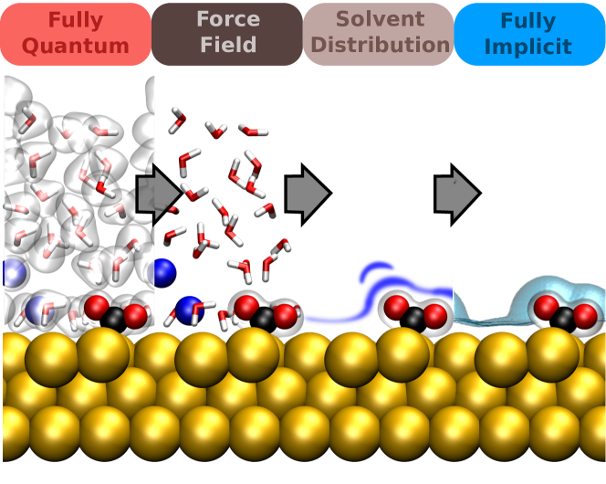
Figure 2: Hierarchy of coarse-graining approaches for the liquid phase in the context of electrocatalysis at SLIs. The sketch depicts an aqueous electrolyte with salt ions (blue spheres) and dissolved CO₂ (red and black molecules) at a crystalline surface. Starting from a fully explicit quantum mechanical description (far left) one can conceptually coarse-grain away electronic DOFs to arrive at a force field or interatomic potential description (center left). From that one can gradually remove nuclear solvent DOFs to represent solvent molecules e.g. only through their spatial distributions or correlation functions like in RISM-type models (center right). Finally, replacing even this with simply a polarizable continuum one arrives at fully implicit models (far right). Note that in the derivation and parametrization of each coarse-grained level one does not necessarily need to follow each step and can e.g. directly parametrize an implicit model from fully explicit data.

The starting point of our discussion is a fully ab initio, quantum mechanical treatment of the liquid phase, including all electronic and nuclear degrees of freedom (DOFs). Given the mobility of the molecules in the liquid phase, the evaluation of equilibrium states requires some sort of averaging or sampling over the nuclear DOFs, most often achieved in the form of ab initio molecular dynamics (AIMD).^{51, 52} Unfortunately, even at this fully explicit level there is still some debate which first-principles electronic structure theory is actually best suited for the task. Specifically for the description of pure water, easily the most important of solvents, there are a number of well documented failures of semi-local DFT,^{53, 54} which in terms of its computational efficiency would be the present-day method of choice to describe larger supercells and achieve longest possible simulation times.^{55, 56} Instead, the use of hybrid DFT with advanced dispersion corrections,^{57, 58} or the strongly constrained and appropriately normed (SCAN) meta-GGA functional^{59, 60} is often recommended, potentially even including nuclear quantum effects.⁶¹ This best practice becomes challenged in the SLI context though—not only because of potentially exploding computational costs, but also because the same functional now has to describe the (metallic) solid and the liquid phase with their very different physical characteristics on the same footing. For this specific task, the use of generalized-gradient functionals, in particular the revised version of the Perdew-Burke-Ernzerhof (RPBE) functional⁶² corrected for dispersion interactions using the semi-emperical D3 approach by Grimme,^{63, 64} is presently often perceived as an acceptable compromise.^{65, 55, 66, 67, 68, 69} However, one clearly has to stress that this consensus derives more from reasonably-appearing averaged properties and functionalities computed at this level of theory, rather than from detailed experimental validation of the predicted atomic-scale structure of the electric DL.

Although AIMD simulations provide valuable insights about SLIs, they can usually only sample a few or even a single basin of the system’s potential energy surface (PES) during presently computationally tractable trajectories on the picosecond time scale. Proper thermodynamic averages would instead require nanoseconds of simulations or longer, especially if the DL contains slowly equilibrating components such as ions or strongly physisorbed water.^{70, 24} Furthermore, the simulation cell sizes feasible even over restricted picosecond time scales can barely, if at all cover the up to $\sim 100$ Å extent of the outer DL, cf. Fig. 1. All these limitations can at present only be overcome by switching to more coarse-grained descriptions especially of the liquid phase as summarized in Fig. 2.

The first in the corresponding hierarchy of approaches focuses on eliminating the electronic DOFs. This results in a classical description of pair-wise or many-body interactions between point-like nuclei in the form of an effective force field or interatomic potential to model the high-dimensional PES.^{71, 72} While this is an extensive field of its own with a plethora of most advanced force fields for (bulk) water, electrolytes or materials, the crux is again in requiring them to describe the SLI within the same simulation cell. Much fewer parametrizations exist for this task, in particular for the interactions of (organic) electrolyte species with the (inorganic and heavy) elements like Pt or Cu that form the metallic electrodes. On top of that, most traditional force fields can not reliably describe bond forming or breaking events and can thus not cover the reactive surface chemistry that is central to catalysis at electrified interfaces. While there are thus only few examples where fully classical simulations were used to study the structure of SLIs,^{73, 74} there are currently two interesting developments to overcome these limitations. To one end, modern reactive force fields that can account for bond dissociation start being applied in SLI simulations ^{75, 76} even under applied potential.^{77, 78, 79, 80} To the other end, machine-learned interatomic potentials are a most promising new possibility to establish a computationally efficient surrogate to direct first-principles calculations.^{81, 82} By construction, their reliability and range of applicability is determined by the training data fed into them. If this data contains appropriate information on the SLI and its reactive events, dynamical simulations based on such a potential would produce the same insight as direct AIMD, just orders of magnitude faster. Precisely the development of corresponding data-efficient training protocols (that would not require prohibitive amounts of first-principles training data) is presently the focus of strong research efforts worldwide. As this research is ongoing, present applications of machine-learned potentials to the SLI context are still restricted to some first case studies though.^{83, 84, 85}

An important general aspect in switching to more coarse-grained descriptions is that different levels may suitably be chosen for different spatial regions of the overall simulation cell. In the SLI context, a widespread realization of such concurrent multiscale modeling is a quantum mechanical/molecular mechanical (QM/MM) approach,^{10, 86, 87, 88, 89, 90} in which the solid electrode and the chemical reactions thereon are kept on a quantum chemical level, while a force field or interatomic potential is employed for the liquid electrolyte. This offers significant speed-ups as much of the electrolyte sampling is done classically, while in particular the reactive surface chemistry is still described at a first-principles level. Note that the (spatial) distinction of what is described at the more coarse-grained level can be chosen flexibly, with the limitation that approaches that allow to continuously morph say a classically described atom into a quantum mechanically described one during an ongoing dynamical simulation are still in their infancy.^{91, 92, 93} Typically, which atoms (or molecules) are described at which level is therefore defined at the onset of a simulation, and this is kept fixed regardless of where the actual dynamical motion drives the atom or molecule to. A classical description of all electrolyte species apart from (specifically) adsorbed reaction intermediates offers thereby obviously highest computational efficiency, but is by construction unable to cover situations where the liquid phase participates actively in the reactions, e.g. as a proton donor.⁸⁷ Furthermore, it also requires in principle specific (interface-sensitive) parametrizations to account for the overall effect of the classical solvent species on the surface reactions. Both of these limitations can instead be mitigated by including (parts of) the inner DL into the quantum mechanical part of the simulation, yet at concomitantly increased computational costs.

Central to the value of such simulations is in any case the correct depiction of the interaction or embedding energy of solid and liquid phase, the solvation energy. In QM/MM models, the Coulomb contribution to the solvation energy is commonly described by the interaction of the QM charge distribution with fixed, fitted electrostatic charges of the classically described liquid molecules. In addition to this, non-Coulomb contributions, including Pauli repulsion, dispersion and induction forces, have to be carefully parametrized.^{88, 89} Electronic induction of the solid phase by the liquid phase charge distribution is treated by self-consistently re-iterating the liquid distribution and electron density.⁸⁶ Polarization of the liquid phase is instead most often only included through movement and reorientation of solvent molecules and ions. In certain situations an additional electronic polarization, i.e. changes of the partial charges of atomic sites of the solvent molecules, has been shown to be relevant and can in principle be included using polarizable force fields.⁹⁴ The description of the other, non-Coulomb interactions is still a topic of ongoing research. Commonly they are simply represented by pairwise interactions with parameters obtained from high-level quantum chemical calculations⁸⁸ or by fitting to thermodynamic or dielectric properties of the (bulk) solvent.⁹⁵ Nevertheless, properly parametrized force fields have actually been shown to sometimes even surpass full AIMD simulations in accuracy concerning structural and dynamic properties of the solvent.⁹⁶ Their still atomistic approach to representing the liquid phase also has advantages over the more coarse-grained models discussed in the following, in that they can more readily describe localized effects and directed interactions such as hydrogen bonds to surface adsorbates.

While a QM/MM description of the SLI greatly speeds up simulations by simplifying the computational treatment of the liquid DOFs,^{97, 87, 98} it still does not relieve the need to sufficiently sample the phase space of each solvent molecule. Combined with the need to still determine the QM polarization response to each new MM charge configuration, even such simplified models might not be computationally tractable. Recognizing the explicit sampling of the solvent dynamics as the bottleneck, a further coarse-graining step aims therefore at effectively averaging out the movement of solvent molecules and ions, and at replacing them instead with their respective spatial equilibrium distributions, cf. Fig. 2. A prominent representative of this ansatz is the reference interaction site model (RISM),⁹⁹ which evaluates the equilibrium radial correlation functions of each pair of species in the system through an analytical integral equation, known as the Ornstein-Zernike equation.¹⁰⁰ Within given approximations,^{101, 102} the equilibrium structure of the fluid around any form of solute is then fully encoded through these radial distribution functions and without further need for a costly dynamical sampling. In most variants of RISM, such as the popular 3D-RISM,¹⁰³ the central pair correlation functions are evaluated on a three-dimensional grid centered on the solute to yield the spatial distribution functions of each solvent site species. These distribution functions can be integrated over space and summed up to yield an excess chemical potential of solvation due to the solute-solvent interaction and solvent reorganization in the presence of the solute. In RISM theory, it is this excess chemical potential that connects the coarse-grained solvent with the explicitly treated solute. Its functional derivative with respect to the electron density yields an effective potential that can directly be included into the solute’s Hamiltonian. This potential includes all the interactions used in the determination of $g_{ij}(\mathbf{r})$ such as electrostatics and, most commonly,¹⁰⁴ Lennard-Jones type terms encompassing dispersion and exchange interactions. Given the implicit dependency of the solvent excess chemical potential on the electron density, the solvent response is then iterated together with the quantum-mechanical DFT-described part of the system to reach self-consistency.¹⁰⁵ Going beyond purely molecular solvents, RISM-like models recently have seen very successful use in the simulations of various electrochemical processes.^{106, 107, 108, 109, 110}

Inherent to effective models, both explicit classical and RISM-based descriptions of the liquid phase depend on a series of element-specific parameters that define interatomic interactions and have to be carefully chosen for each system of interest. This requirement is generally not a significant burden for detailed studies of individual systems, in particular if these are prototypical cases for which then typically a plethora of high-level or experimental data is available that can be used for the parametrization. It becomes critical though, if fast estimates are needed, for instance to assess the catalytic activity of a large variety of electrode materials, morphologies, active sites or electrolyte components, or if unknown and complex electrochemical reactions are studied for which no reference data is available. For such cases and for potential further increases in efficiency, an even higher level of coarse graining of the liquid phase becomes appealing, in which all solvent DOFs are altogether merely described via a polarizable continuum, cf. Fig. 2.

Following the concurrent multiscale modeling philosophy of QM/MM or QM/RISM, such implicit solvation schemes are in the SLI context predominantly employed to describe the equilibrium solvent response on a (metallic) electrode computed at a first-principles level of theory. Again, flexibility exists whether to replace the entire electrolyte in a so-called fully implicit approach, or to retain an explicit quantum or molecular mechanical description of (parts of) the inner DL, with latter models referred to as hybrid explicit/implicit models. Reduced to a continuum, the implicitly treated electrolyte is then just a polarizable medium with a dielectric permittivity. While an isotropic, constant tensor in the bulk of the electrolyte, this permittivity can in principle vary closer to the symmetry-breaking SLI. Additionally, it needs to be artificially reduced to vacuum permittivity inside the explicitly treated region of the simulation cell so as to not introduce spurious polarizability on top of the one intrinsically provided by the quantum or molecular mechanical description of the corresponding atoms or molecules. This region of vacuum permittivity inside the overall simulation cell is commonly referred to as solvation cavity, a word coined within the traditional field of implicit solvation of finite moleculear solutes. As discussed in detail in Section 2.3, different classes of implicit solvation schemes are categorized by the functional form employed to describe these spatial variations of the dielectric permittivity tensor. This form determines the electrostatic solvent response and could in principle be chosen to be non-local to reach similar levels of accuracy as RISM models.¹¹¹ However, the use of such functional forms would unavoidably require the introduction of a multitude of system-specific parameters, thereby nullifying the original motivation for this effective methodology.

For planar electrodes (typically described by crystalline slabs with low-index surfaces in the corresponding first-principles supercell calculations), it is therefore common to only consider a local and stationary dielectric tensor with components that vary exclusively as a function of the vertical distance $z$ to the surface.¹¹² In fact, typically even the tensorial nature of the permittivity is neglected and a simple functional form for the scalar permittivity $\epsilon(z)$ is employed. As this omits all structure in the liquid and especially any kind of directed interactions with the surface, such effects are instead considered by additional effective non-Coulomb energy functionals as discussed in more detail in Section 2.4 below. This particular strategy then allows to employ a minimum number of parameters for the dielectric modeling function and these non-Coulomb energy corrections as further discussed in Section 2.6.

We also discuss prevalent fitting strategies for these parameters in Section 2.6, but note already here that the simplicity of this prevalent approach does not only reflect the objective of creating a computationally most effective, transferable solvation approach. To some extent and as mentioned before it is also dictated by the present scarcity of interface-sensitive experimental or high-level theoretical reference data that does not warrant a more detailed (physical) modeling with a concomitantly increased number of parameters. This aspect notably also concerns the powerful possibility of extending implicit solvation schemes from pure liquids to electrolytes by additionally modeling the ionic charge distribution as discussed more in Section 2.5. Most of these models rely on the traditional diffuse DL theory, providing a functional form between ion distributions and electrostatic potential as developed by Gouy, Chapman and Debye in the beginning of the last century.^{113, 114, 115, 116, 117} Since this original approach, many corrections regarding e.g. non-mean-field ionic correlation effects, steric size corrections or ion-surface interactions have been made. While physically clearly motivated, each of these corrections necessarily gives rise to further parameters. Even though it is in particular this capability to account for the ionic counter charges that is presently predominantly exploited for the SLI context, it is thus again a specific issue of this application field in how much these more advanced electrolyte models can be parametrized or are in fact really necessary for the specific counter charge modeling aspect.

2.2 Separation of the grand potential energy functional

As apparent from the discussion in the last section, different levels of theory ranging from high-level quantum chemistry to force fields or interatomic potentials may generally also be chosen for the description of the solid electrode (and an explicitly treated part of the inner DL). In the remainder of this review we will nevertheless focus on the use of DFT for this task, as this is the predominantly taken approach in implicit solvation works on SLIs and electrocatalysis at metallic electrodes to day.²⁰ With minor modifications, many of the concepts and discussions are readily adapted to the other levels of theory though.

As described in the introduction around Fig. 1, in the SLI context, the employed DFT supercell at volume $V$ generally only represents a grand-canonical sub-system, which is connected to bulk reservoirs of species that represent the rest of the (macroscopic) system. For the electrochemical environment, these would naturally include an electrochemical potential $\tilde{\mu}_{\rm el}$ for the electrons, electrochemical potentials $\tilde{\mu}_{{\rm ion},i}$ for different ionic electrolyte species $i$, and chemical potentials $\mu_{{\rm solv},j}$ for different neutral solvent species $j$. In Chapter 3 we will detail how these potentials are set for the SLI context, but for the time being they are simply given constants. For such given constants, the true equilibrium structure and composition of the electrified interface would result from an exhaustive grand-canonical sampling and thermodynamic averaging of all nuclei and electronic DOFs inside the supercell—with nuclei DOFs here and henceforth denoting the detailed geometric structure and chemical composition of the system and electronic DOFs referring to those of the DFT-part of the system. In the coarse-grained solvation modeling reviewed here, this typically infeasible task is separated into two stages. First, solvation effects are evaluated for an individual interface configuration characterized by say a given electrode geometry and chemical composition with specifically adsorbed reaction intermediates at its active sites. The chemical composition $N_{\alpha}$ of chemical species $\alpha$ in this explicitly and DFT-described part of the system is thus fixed, and under an unanimous Born-Oppenheimer approximation the thermodynamic sampling and averaging is restricted to the remaining (canonical) electronic and (grand-canonical) nuclei DOFs of the electrolyte. In other words, one thus evaluates the thermodynamic stability of the electronic ground-state configuration for the given static nuclei charge density $\rho_{\rm nuc,QM}=\rho_{\rm nuc,QM}({\bf r})$ and in contact with a fully equilibrated electrolyte. In a subsequent step detailed in Section 3.1, an ab initio thermodynamics framework is then employed to compare the stability of different such explicit interface configurations and compositions, and the one exhibiting the highest stability is identified as the closest approximant to the true grand-canonical equilibrium SLI structure within the tested space of configurations.

In this and the remaining sections of this chapter we will concentrate on the first of these two stages. In this stage, there is thus one defined chemical composition $N_{\alpha}$ of the DFT-described part of the system, and in this respect this stage then encompasses the more traditional use of implicit solvation schemes in the molecular DFT context with finite solutes. The central ansatz taken to accomplish the thermodynamic evaluation at this stage is to partition the overall system’s energy, and establish a grand potential energy functional of the charge density distribution $\rho_{\rm is}=\rho_{\rm is}({\bf r})$ of the classical electrolyte and the electron density $\rho_{\rm el,QM}=\rho_{\rm el,QM}({\bf r})$ of the DFT-described part

$$\Omega^{N_{\alpha}}[\rho_{\mathrm{el,QM}},\rho_{\rm is}] =\left.F_{\mathrm{QM}}\left[\rho_{\mathrm{el,QM}}\right]\right|_{\rho_{\rm nuc,QM}}\;+\;\Omega_{\mathrm{is}}[\rho_{\mathrm{el,QM}},\rho_{\rm is}]\quad,$$ (1a)

which is minimized by the equilibrated charge density distribution $$\rho^{\circ}_{\rm is} \rho^{\circ}_{\rm el,QM} F_{\mathrm{QM}} \Omega_{\mathrm{is}} F_{\mathrm{QM}}\rightarrow F F \rho_{\rm nuc} F$$ and the ground-state electron density . Here, is the free energy functional of the pure quantum system and is the grand potential of the surrounding electrolyte. For simplicity of notation, we drop in the following the subscript “QM” (e.g. ), and consistently denote all properties related to the electrolyte with the subscript “is” (for implicit solvent). Within the employed Born-Oppenheimer approximation, we also henceforth refrain from explicitly stating the only parametric dependence of on the nuclei charge density . Within Kohn-Sham (KS) DFT, is commonly expressed as

$$F[\rho_{\mathrm{el}}] =\underbrace{\overbrace{\mathcal{T}^{\mathrm{S}}_{\mathrm{el}}[\rho_{\mathrm{el}}]+\mathcal{V}^{\mathrm{mf}}[\rho_{\mathrm{el}}]+E^{\mathrm{xc}}[\rho_{\mathrm{el}}]}^{E^{\mathrm{KS}}[\rho_{\mathrm{el}}]}+\mathcal{T}_{\mathrm{nuc}}[\rho_{\mathrm{el}}]}_{U[\rho_{\mathrm{el}}]}-TS[\rho_{\mathrm{el}}]\quad.$$ (1b)

Here, $$\mathcal{T}_{\mathrm{el}}^{\mathrm{S}} \mathcal{T}_{\mathrm{nuc}} \rho^{\circ}_{\rm el} \mathcal{V}^{\mathrm{mf}} E^{\mathrm{xc}} E^{\mathrm{KS}} TS T F U$$ is the kinetic energy functional of the non-interacting electrons and represents the kinetic energy functional of the nuclei (usually evaluated only as a post-correction at ). The Coulomb energy functional contains both nuclei-nuclei interactions described explicitly and electronic interactions described on the mean-field level, while additional electronic interactions are accounted for through the DFT exchange-correlation functional . is generally referred to as the KS energy functional, and finally, represents entropic corrections at the given temperature . As indicated, all terms in with the exception of the last one are often summarized under the header of the internal energy functional .

Importantly, $F[\rho_{\mathrm{el}}]$ with all its terms is exactly the functional also underlying regular DFT calculations and does thus not depend on the electrolyte distribution $\rho_{\rm is}$. We correspondingly refer to a multitude of excellent accounts on KS DFT for further details on this functional.¹¹⁸ All electrolyte-induced changes of the ground-state electron density arise instead from the optimization of the grand potential $\Omega^{N_{\alpha}}[\rho_{\mathrm{el}},\rho_{\rm is}]$ in eq. (1a) and not $F[\rho_{\mathrm{el}}]$ alone. In contrast, $\Omega_{\mathrm{is}}[\rho_{\mathrm{el}},\rho_{\rm is}]$ as the second part of this grand potential refers to the electrolyte in its equilibrium distribution, and this does depend on the detailed charge distribution of the DFT-described solute and thus its electron density $\rho_{\rm el}$. Conceptually, in order to determine $\Omega_{\rm is}[\rho_{\mathrm{el}},\rho_{\rm is}]$ all electrolyte DOFs would therefore have to be sampled in the presence of a given $\rho_{\rm el}$, and then the interdependence of electrolyte and DFT system charge densities would require an iterative cycle or generally a numerical optimizer to minimize the functional $\Omega^{N_{\alpha}}[\rho_{\mathrm{el}},\rho_{\rm is}]$ with respect to the electron density at a corresponding equilibrium charge density distribution of the electrolyte. This has e.g. been realized in electrostatic QM/MM embedding,^{86, 87} where molecular dynamics simulations are used to sample the equilibrium distributions of the electrolyte DOFs. Similarly QM/RISM simulations have been employed, in which a more coarse-grained model is used to derive the electrolyte equilibrium distribution corresponding to a given electron density of the QM system¹⁰⁵ as already mentioned in Section 2.1.

The great advantage of implicit solvation schemes over these less coarse-grained approaches is that there a model solvation grand potential $\Omega_{\rm is}[\rho_{\mathrm{el}}]$ is derived solely as an explicit functional of the electron density $\rho_{\mathrm{el}}$. This leads to a dramatic reduction of computational effort, as then the evaluation of the resulting closed form of $\Omega^{N_{\alpha}}[\rho_{\mathrm{el}}]$ can be achieved for a given $\rho_{\mathrm{el}}$ in one go. In fact, corresponding schemes are often directly integrated into the DFT program packages by simply adding routines that evaluate and add the $\Omega_{\rm is}[\rho_{\mathrm{el}}]$ contribution within the regular KS DFT minimization procedure. For this, it seems at first natural to separate the model grand potential functional into formal terms analogous to the quantum free energy functional $F[\rho_{\mathrm{el}}]$,

$$\Omega_{\mathrm{is}}[\rho_{\mathrm{el}}]=\underbrace{\mathcal{T}_{\mathrm{is}}[\rho_{\mathrm{el}}]+\mathcal{V}_{\mathrm{is}}[\rho_{\mathrm{el}}]}_{U_{\mathrm{is}}[\rho_{\mathrm{el}}]}-TS_{\mathrm{is}}[\rho_{\mathrm{el}}]-\sum_{i}\tilde{\mu}_{\mathrm{ion},i}\langle N_{\mathrm{is,ion},i}\rangle[\rho_{\mathrm{el}}]-\sum_{j}\mu_{\mathrm{solv},j}\langle N_{\mathrm{is,solv},j}\rangle[\rho_{\mathrm{el}}]\quad,$$ (1c)

with the respective kinetic, potential and internal energy functionals $\mathcal{T}_{\mathrm{is}}$, $\mathcal{V}_{\mathrm{is}}$ and $U_{\mathrm{is}}$, and the entropic contribution denoted by $S_{\mathrm{is}}$. Note that as a grand potential, $\Omega_{\mathrm{is}}$ formally also contains contributions due to the electrochemical potentials of the ionic ($\tilde{\mu}_{\mathrm{ion},i}$) and chemical potentials of the neutral solvent species ($\mu_{\mathrm{solv},j}$). The inclusion of these terms—and especially their average particle numbers $\langle N_{\mathrm{is,ion},i}\rangle$ and $\langle N_{\mathrm{is,solv},j}\rangle$ in the implicit electrolyte—does at first seem counter-intuitive given that all explicit solvent and ion degrees of freedom have been coarse-grained out. Yet, as we will see below, even implicit ionic and solvent molecule concentrations in the simulation box depend on the electrochemical environment (e.g. the applied potential). Therefore the exchange of both kinds of particles with the extended electrolyte (as represented by the (electro)chemical potentials) needs to be accounted for, at least approximately.

In general, and as further elaborated on in Section 3.1, one is actually rarely interested in the absolute grand potential of eq. (1a). Instead it is differences in free energies, and thus differences in grand potentials at their respective optimal electronic densities, that are the main descriptors of chemical reactions. Similarly, comparisons with experiment—which are generally used for model parametrization—are also most easily done on the level of solvation free energies,¹¹⁹ which in turn are differences between the grand potential at optimized densities in solvent and in vacuum. For this purpose and considering the strong approximations to be made anyway, the fine separation into the various formal terms in eq. (1c) is not ideal. With the aim to later on exploit partial cancellations and to ultimately create computationally most tractable terms, it has instead proven more convenient to group the different contributions by their physical origin²⁸

$$\Omega_{\rm is}[\rho_{\mathrm{el}}]=\mathcal{V}_{\mathrm{is}}^{\mathrm{mf}}[\rho_{\mathrm{el}}]+\Omega_{\mathrm{is}}^{\mathrm{non-el}}[\rho_{\mathrm{el}}]+\Omega_{\mathrm{is}}^{\rm ion}[\rho_{\mathrm{el}}]\quad.$$ (2)

Here, $\mathcal{V}_{\mathrm{is}}^{\mathrm{mf}}$ is the mean-field contribution due to the electrostatic response of the continuous polarizable medium describing the pure liquid. Interactions with the pure liquid beyond this mean-field electrostatics are accounted for by the second term, which summarizes a number of so-called non-electrostatic contributions

$$\Omega_{\mathrm{is}}^{\mathrm{non-el}}[\rho_{\mathrm{el}}]\;=\;\Omega_{\mathrm{is}}^{\rm cav}[\rho_{\mathrm{el}}]+G_{\mathrm{is}}^{\rm rep}[\rho_{\mathrm{el}}]+G_{\mathrm{is}}^{\rm dis}[\rho_{\mathrm{el}}]+G_{\mathrm{is}}^{\rm tm}[\rho_{\mathrm{el}}]\quad,$$ (3)

while the last term $\Omega_{\rm is}^{\rm ion}[\rho_{\mathrm{el}}]$ in eq. (2) describes all additional effects introduced by ions in the electrolyte. Even though in practice often further lumped together, cf. Section 2.6, we here distinguish four non-electrostatic contributions. $\Omega_{\mathrm{is}}^{\rm cav}[\rho_{\mathrm{el}}]$ denotes the grand potential cost of forming a cavity in the solvent for the solute to be placed in. Making this space for the solute necessarily changes the particle numbers of solvent molecules of the implicitly-described liquid in the supercell and thus involves particle exchange with the reservoirs with a concomitant dependence on the chemical potentials of the solvent components. We accordingly denote this term here as a grand potential, even though most available literature refers to it as a cavitation free energy functional. $G_{\mathrm{is}}^{\rm rep}[\rho_{\mathrm{el}}]$ commonly represents the contribution due to exchange or Pauli repulsion interactions, effectively also including an entropic contribution due to the resulting changes to the potential energy surface (PES). The third term, $G_{\mathrm{is}}^{\rm dis}[\rho_{\mathrm{el}}]$, similarly represents dispersion or van der Waals interactions. Finally, $G_{\mathrm{is}}^{\rm tm}[\rho_{\mathrm{el}}]$ is the free energy functional accounting for changes in the thermal motion of the solute. Note that all of the non-electrostatic terms and $\Omega_{\rm is}^{\rm ion}[\rho_{\mathrm{el}}]$ thus contain potential, kinetic and entropic contributions. Nevertheless, each of these terms has been proven to be computationally accessible and in the following sections, we will now further elaborate on these various contributions to $\Omega_{\rm is}[\rho_{\mathrm{el}}]$, starting first with a pure solvent and the discussion of the dominant electrostatic $\mathcal{V}_{\mathrm{is}}^{\mathrm{mf}}[\rho_{\mathrm{el}}]$ term in Section 2.3 and the non-electrostatic $\Omega_{\mathrm{is}}^{\mathrm{non-el}}[\rho_{\mathrm{el}}]$ in Section 2.4. In Section 2.5, ions are then added on top of that to arrive at full implicit electrolyte models that also include a model $\Omega_{\rm is}^{\rm ion}[\rho_{\mathrm{el}}]$ grand potential. The general objective in all of these sections is to derive (closed) expressions for these functionals of the electron density, which then allows to (straightforwardly) add these contributions into the KS DFT minimization process. As noted before, the true free energy is then formally given by the grand potential $\Omega^{N_{\alpha}}[\rho^{\circ}_{\mathrm{el}}]$ evaluated at the resulting optimized density $\rho^{\circ}_{\mathrm{el}}$, cf. eq. (2.2a). However, it is important to note that, to this end, the practical implementations acknowledge the aforementioned fact that predominantly only grand potential energy differences are required. In such differences of say systems $A$ and $B$,

$$\Delta\Omega(A,B)\;=\;\Omega^{A}[\rho^{\circ}_{\mathrm{el}}(A)]-\Omega^{B}[\rho^{\circ}_{\mathrm{el}}(B)]\quad,$$ (4)

contributions to $\Omega_{\rm is}[\rho_{\mathrm{el}}]$ that are not particularly sensitive to the detailed form of the optimized densities $\rho^{\circ}_{\mathrm{el}}(A)$ and $\rho^{\circ}_{\mathrm{el}}(B)$ will largely cancel. From this perspective, no efforts are therefore made to account for such contributions in the derived functional expressions in the first place. While formally describing the absolute solvation grand potential of eq. (2), we thus emphasize that in practice many of the expressions discussed in the next sections only work for free energy differences. In fact, not least for reasons of computational efficiency the practical implementations often also consider only some terms within $\Omega_{\rm is}[\rho_{\mathrm{el}}]$ in the functional minimization. One justification for this is an assumed negligible impact of the omitted terms on the final optimized electron density. Another pragmatic one is that any error incurred through the omission is effectively compensated in the fitting of the model parameters to reference data.¹²⁰ A prominent example for this is to only consider the electrostatic $\mathcal{V}_{\mathrm{is}}^{\mathrm{mf}}[\rho_{\mathrm{el}}]$ in the minimization, and evaluate all non-electrostatic free energy contributions only as a post-correction on the basis of the resulting electron density that was thus exclusively optimized with respect to the dominant mean-field polarization effect of the surrounding liquid.

2.3 Electrostatics of solvation

2.3.1 Potential energy and polarization models

The mean-field electrostatic $\mathcal{V}_{\mathrm{is}}^{\mathrm{mf}}$ is the contribution to the solvation grand potential most intuitively associated with the response of a solvent to a solute. Considering it jointly with the Coulomb energy functional $\mathcal{V}^{\rm mf}$ in the minimization of the grand potential energy functional of eq. (1a) accounts for the polarization response of the continuum solvent to the net charge distribution of the solute $\rho$ (resulting from the electron $\rho_{\mathrm{el}}$ and nuclei $\rho_{\mathrm{nuc}}$ charge densities of the DFT part of the system) and vice versa. To derive this contribution, we consider the static displacement field $\boldsymbol{D}$ which arises from the collection of these explicit charges in the system and is screened by the surrounding medium. $\boldsymbol{D}$ is given by the generalized Poisson equation (GPE)¹²¹

$$\nabla\boldsymbol{D}=\left(\rho_{\mathrm{el}}+\rho_{\mathrm{nuc}}\right)\quad.$$ (5)

The displacement field is related to the electric field $\boldsymbol{E}$ of the explicit charge distribution via the polarization vector $\boldsymbol{P}$, representing permanent and induced dipoles in the system. The functional form of $\boldsymbol{P}$ is generally quite complicated, but depends on the relative and generally non-local dielectric permittivity tensor $\boldsymbol{\varepsilon}=\boldsymbol{\varepsilon}_{\mathrm{tot}}/\varepsilon_{0}$ (with the absolute $\boldsymbol{\varepsilon}_{\mathrm{tot}}$ and vacuum permittivity $\varepsilon_{0}$),

$$\boldsymbol{D}=\varepsilon_{0}\boldsymbol{E}+\boldsymbol{P}[\boldsymbol{E},\boldsymbol{\varepsilon}]\quad.$$ (6)

Technically, this makes $\boldsymbol{D}$ a functional of the electric field $\boldsymbol{E}$, which itself is an implicit functional of the net charge density ($\rho_{\mathrm{el}}+\rho_{\mathrm{nuc}}$) via eq. (5). For reasons of legibility we dropped these dependencies though. In this definition of $\boldsymbol{D}$, the permittivity tensor is assumed to be static—i.e. time independent, but may still vary in space, e.g. to account for the symmetry breaking through a finite solute or an extended interface. Note that eq. (6) also omits higher-order multipolar terms that might arise in the medium. For water, this approximation is generally well justified because the solvent molecules’ electric field is dominated by its dipole moment. Higher-order terms can, however,¹²² be important in non-aqueous solvents with sizeable higher-order multipole moments, but to our knowledge no DFT program package yet supports an implicit solvent parametrization including such higher-order terms.

The GPE of eqs. (5) and (6) provides a direct relation of electric field and charge density which is generally valid, with and without a polarizable medium. It can be used to find an analytic expression for the electrostatic Coulomb potential energy contribution of an arbitrary embedded charge distribution

$$\left(\mathcal{V}^{\mathrm{mf}}+\mathcal{V}_{\mathrm{is}}^{\rm mf}\right)[\rho_{\mathrm{el}}]=\frac{1}{2}\int\left(\rho_{\mathrm{el}}+\rho_{\mathrm{nuc}}\right)\phi=\frac{1}{2}\int\boldsymbol{E}\boldsymbol{D}\mathrm{d}\boldsymbol{r}\quad,$$ (7)

where the last equation can be obtained from inserting eq. (6) into eq. (5), using the divergence theorem, neglecting the surface terms and finally substituting $\boldsymbol{E}=-\nabla\phi$, with $\phi$ the electrostatic potential.

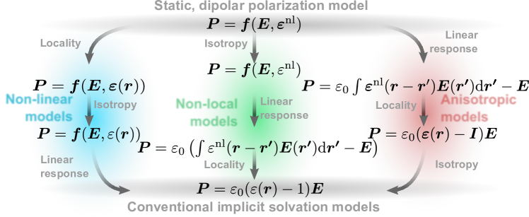
Figure 3: Categorization of different electrostatic solvation models. From the general starting point of a static non-linear, non-local and anisotropic model (top) several approximations can be made to ultimately arrive at the linear, local and isotropic polarization model most commonly applied in present-day DFT codes.

The assumption of a static, i.e. frequency independent, dielectric permittivity implies that the solvent adapts instantaneously to the electron and nuclei charge distribution of the solute. While this is generally a good approximation for the solvent response on thermodynamic equilibrium and potentially even for transition states of chemical reactions, it will over-screen fast molecular dynamics, such as vibrations or charge-transfer processes.⁴⁷ On top of that, the simulation of electronically excited states has been shown to generally also necessitate a frequency-dependent dielectric response.^{123, 124} For most other cases, however, the static, dipolar response model is a good starting point for further approximations. As compiled in Fig. 3, these lead to three main categories of dielectric models, namely non-linear, non-local and anisotropic ones. Non-linearity in the solvent response can be important in cases where the electric field is large, which actually can be the case inside the electric DL.^{21, 125} Notwithstanding, mostly a Taylor expansion of $\boldsymbol{P}$ as a function of $\boldsymbol{E}$ around $\boldsymbol{E}=0$ can be truncated after the linear term (linear-response approximation), i.e.

$$\boldsymbol{P}\approx 0+\varepsilon_{0}\left({\boldsymbol{\varepsilon}}-\boldsymbol{I}\right)\boldsymbol{E}\quad,$$ (8)

with the medium’s electric susceptibility directly expressed as $({\boldsymbol{\varepsilon}}-\boldsymbol{I})$.¹²¹ Next, non-locality in the solvent response is important, whenever solvent molecule correlations occur, e.g. close to charged solutes. The spherically averaged liquid susceptibility (SaLSA) model represents one example that accounts for non-locality.¹¹¹ SaLSA has been also coarse-grained into a computationally more feasible local version (charge-asymmetric nonlocally determined local-electric, CANDLE), with the dielectric permittivity being derived from the non-local response.¹²⁶ Non-locality may also be employed to account for an effective size of solvent molecules, since the electric field at a certain position then affects the solvent density in a finite solvent radius around it.¹²⁷ This can be relevant to prevent solvent from penetrating into small pockets formed by the solute, see the discussion on the dielectric function below. Finally, anisotropic properties of the dielectric permittivity are, of course, generally important in systems with reduced symmetry. This is notably the case at electrified SLIs where even at a planar interface the dielectric tensor would at least feature two independent dielectric tensor components, parallel $\varepsilon_{||}$ and vertical $\varepsilon_{\perp}$ to the surface.¹²⁸

While non-linearity, non-locality and anisotropy could thus well be of relevance for SLIs, most implicit solvation models that have been implemented into DFT program packages to date neglect all three of them and are based on the most simple case of a linear, local and iosotropic dielectric model $\varepsilon({\bf r})$. For this case, the GPE becomes

$$\nabla\boldsymbol{D}=\varepsilon_{0}\nabla\left[\varepsilon(\boldsymbol{r})\boldsymbol{E}\right]=-\varepsilon_{0}\nabla\left[\varepsilon(\boldsymbol{r})\nabla\phi\right]=\left(\rho_{\mathrm{el}}+\rho_{\mathrm{nuc}}\right)$$ (9)

and the electrostatic Coulomb potential energy of eq. (7) can be further simplified. Using eq. (8), it then features separately the electrostatic energy functional contributions of the DFT part and of the implicit solvent

$$\left(\mathcal{V}^{\mathrm{mf}}+\mathcal{V}^{\rm mf}_{\mathrm{is}}\right)[\rho_{\mathrm{el}}]=\frac{1}{2}\int\left(\rho_{\mathrm{el}}+\rho_{\mathrm{nuc}}\right)\phi=\underbrace{\frac{\varepsilon_{0}}{2}\int\boldsymbol{E}^{2}\mathrm{d}\boldsymbol{r}}_{\mathcal{V}^{\mathrm{mf}}}+\underbrace{\frac{1}{2}\int\varepsilon_{0}\left(\varepsilon({\boldsymbol{r}})-1\right)\boldsymbol{E}^{2}\mathrm{d}\boldsymbol{r}}_{\mathcal{V}^{\rm mf}_{\mathrm{is}}}\quad,$$ (10)

with $\phi$ an implicit functional of $\rho_{\mathrm{el}}$ via eq. (9). Since the latter GPE cannot be solved analytically for most dielectric functions, a closed form is typically not attainable and a numerical solution is required. Common methods for this include fixed point iterations or the conjugate gradient technique employing the analytically known Green’s function of the Poisson equation in vacuum.^{129, 130} Alternatively, for certain functional forms of the dielectric function multi-center multipole expansions have been shown valuable,¹³¹ or mappings onto a finite grid and solution via standard finite difference or finite element techniques. Regardless of this technical realization, the conceptual changes to a DFT code to incorporate the Coulomb electrostatic contribution at this level of dielectric model are nevertheless minimal. In fact, while the entire self-consistency cycle around the KS equations is untouched, the only change is that the electrostatic potential does no longer satisfy the normal Poisson equation, but is instead given by the GPE of eq. (9).¹³²

2.3.2 Dielectric function

For the linear, local and isotropic case, the dielectric permittivity $\varepsilon({\bf r})$ may generally still vary in space. As already introduced in Section 2.1, in present-day implicit solvation schemes this is primarily reduced to modeling a transition from the bulk solvent permittivity $\varepsilon_{0}\varepsilon_{\infty}$ (with the relative solvent permittivity $\varepsilon_{\infty}$) deep inside the electrolyte to the vacuum permittivity $\varepsilon_{0}$ inside the DFT-described part of the supercell. The optimum location and form of this transition is generally system specific. Optimum refers hereby to the best possible reproduction of the true solvation effects within the confines of the chosen dielectric continuum model, and—in particular in the widespread approach to even include the inner DL fully into the implicit model—system specific includes an actual dependency on the electrode structure and chemical composition. In principle, this optimum location and form for a specific system could be determined from high-level explicit simulations.¹²⁸ However, this would negate the original motivation to use an implicit solvent model for its efficiency gain and to e.g. screen a large number of different SLIs. Implicit solvation schemes rely therefore typically on a sufficiently simple functional form of $\varepsilon({\bf r})$ which includes as much system-relevant physics as possible while maintaining an optimum transferability. Obviously, this implies a trade-off between a more physically accurate description for particular systems (then typically involving a larger number of parameters that need to be determined) and a more simplified model with as little parameters as possible to describe qualitative trends over a wide range of systems.

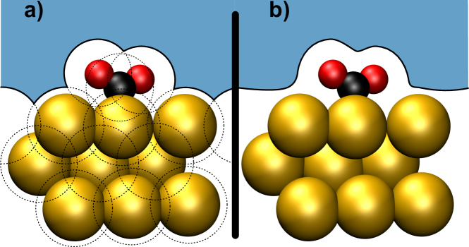
Figure 4: Illustration of different types of dielectric transition between solute and solvent. For the example of an adsorbed CO₂ molecule at a single-crystal surface, a) shows the solvation cavity resulting from the superposition of atom-centered spheres based on eq. (11), while b) shows the solvation cavity as defined by an isosurface of the electron density.

Favoring higher transferability, the dielectric transition is often approximated by a mere switching function between bulk solvent and vacuum, resulting in the formation of a solvation cavity. The location of the dielectric transition thereby has to be expressed in an appropriate molecular descriptor that is readily available in any DFT calculation. For this and as illustrated schematically in Fig. 4, traditional implicit solvation techniques as dominantly used in molecular chemistry often rely on defining a solvation cavity by summing up atom-centered shape functions $s({\bf r})$, so that

$$\varepsilon(s(\boldsymbol{r}))=\left(\varepsilon_{\infty}-1\right)\left\{\prod_{\alpha}s_{\boldsymbol{r}}(|\boldsymbol{r}-\boldsymbol{R}_{\alpha}|,\boldsymbol{\mathcal{P}}_{\alpha})\right\}+1\quad.$$ (11)

Here $s_{\boldsymbol{r}}$ is a shape function going from 0 in the solute region to 1 in the bulk electrolyte, $\{\boldsymbol{R}_{\alpha}\}$ are the positions of the nuclei, and $\boldsymbol{\mathcal{P}}_{\alpha}=(\{r_{\alpha}\},\dots)$ is a vector of parameters, containing e.g. the exclusion radius $r_{\alpha}$ for each atom and the transition smoothness of the shape function. The simplest shape function is just a single Heaviside function $s_{\boldsymbol{r}}=\theta(|\boldsymbol{r}-\boldsymbol{R}_{\alpha}|-r_{\alpha})$, with the atomic radii $r_{\alpha}$ as the only parameters. These radii are usually either taken as tabulated van der Waals radii for each chemical element or fitted to reproduce some experimental data as discussed in more detail in Section 2.6. One advantage of using such a sharp step function, also sometimes referred to as apparent surface charge approach, is the efficiency with which the GPE can be solved using boundary element methods. Yet, in most cases¹³¹ this comes at the expense of additional approximate corrections for errors due to parts of the QM charge density lying beyond the transition. Corrections for this outlying-charge error are correspondingly integral parts of well-known implicit solvation approaches like the polarizable continuum model (PCM),²⁸ the solvent model (SMx),¹³³ or the conductor-like screening model (COSMO)¹³⁴ that rely on such sharp step functions. As an alternative, recently also smoothed step functions were proposed and adapted specifically for SLI simulations (soft-sphere continuum solvation - SSCS model¹³⁵), then, however, requiring additional parameters for the functional form of this transition.

In general, defining the cavity based on atom-centered shape functions has the advantage of easily being able to implement dielectric regions, e.g. at dielectric interfaces, by assigning different values to the local dielectric permittivity. Additionally, solvation radii can be assigned separately to each atom based on their chemical environment. This allows for great flexibility in the definition of the dielectric function and, potentially, a more accurate prediction of solvation energies. Unfortunately, such a treatment also results in a larger parameter space, risking overfitting¹¹⁹ with the generally rather small available training sets as further discussed in Section 2.6. Furthermore, the reliance on atom-centered shapes may lead to the formation of encapsulated solvent pockets in lower-density parts of the solute.¹²⁷ In particular in the context of extended metallic electrodes, filling such pockets with solvent unlikely reflects the correct physics.

Both of these limitations may be overcome in a different, equally popular approach. It recognizes that the presence of electron density—readily available in a DFT calculation—naturally separates explicitly treated regions from the rest of the supercell. The solvation cavity can thus be defined by an iso-surface of the electron density. Regions of lower $\rho_{\rm el}$ than the chosen iso-value are then classified as the solvent, while regions of higher $\rho_{\rm el}$ obviously represent the DFT-treated part of the system. In practice, smoothed shape functions are employed,

$$\varepsilon(\rho_{\mathrm{el}}(\boldsymbol{r}))=(\varepsilon_{\infty}-1)s_{\rho_{\mathrm{el}}}\left(\rho_{\mathrm{el}}(\boldsymbol{r}),(\rho_{\mathrm{el,min}},\rho_{\mathrm{el,max}})\right)+1\quad,$$ (12)

where $\rho_{\mathrm{el,min}}$ and $\rho_{\mathrm{el,max}}$ are the minimal and maximum electron density between which the shape function $s_{\rho_{\mathrm{el}}}$ switches from bulk solvent to vacuum. This kind of parametrization has for instance been employed in the self-consistent continuum solvation (SCCS) model by Andreussi et al.¹²⁹. Equivalently, also the iso-value itself could be used as parameter, with the transition width then as corresponding second parameter.^{136, 137} Various smooth shape functions have been proposed in the literature,^{129, 138, 135} resulting, however, in quite similar predictive accuracy of molecular solvation energies. While this suggests the actual shape to be less influential for the model performance, some functions like the one proposed in the SCCS model are constructed to have an exactly zero gradient outside the transition region, which is beneficial for the numerical solution.^{129, 130} The advantage of the electron density based approach in general is that the solvation cavity adapts self-consistently to the electron density and exhibits thus a more physically reasonable and smooth shape.¹²⁹ From a technical standpoint, though, dielectric functions based on the electron density are slightly more involved to implement due to additional Pulay forces arising there.¹³²

Both, atom-centered shape function and electron density based approaches are generally challenged in the description of solutes at different charge states. In the molecular context, different parameter sets defining the solvation cavity are often required for anions on the one hand, and cations and neutral molecules on the other.¹³⁹ To overcome this limitation, Sundararaman et al. proposed an extended form of the dielectric function,¹³⁸ that in addition to defining the transition region via the electron density allowed for a correction based on the locally averaged outward electric field. This field has inverse signs for cation- and anion-like regions, and thus provides the model with the fundamental capability to shift the dielectric transition region accordingly without the need to invoke different parameters. A similar approach has recently been followed by Truscott and Andreussi,¹⁴⁰ who utilized the SSCS atom-centered shape function model and allowed the atomic spheres to relax their radius depending on the value of the electric field flux through their surface.

2.4 Non-electrostatics of solvation

The interaction between solute and solvent is not solely restricted to the electrostatic mean-field treatment described in the last section, even though especially for the study of electrified interfaces changes in the electrostatic potential can be expected to be dominant.²⁸ Nevertheless, it is often minute changes to free energy profiles of reactions at these interfaces that can result in crucial changes of the catalytic activity or in particular of catalytic selectivities—and for such minute changes the additional beyond mean-field and non-electrostatic interactions could prove decisive. In this section we discuss the corresponding terms in the solvation grand potential, cf. eq. (3), the physical background for them and how they are commonly treated. As will become apparent, this treatment is generally highly effective and thus incurs in principle multiple additional parameters. Not least from a parametrization point of view, but also for reasons of computational efficiency and to exploit potential error cancellation, modern implementations in DFT packages therefore rarely calculate these terms individually.²⁸ Instead, some or all of these terms are instead lumped together into empirical functions with a minimum number of parameters. Highly successful examples for this are the SMx²⁹ family of methods or the SCCS approach.¹²⁹ As it is important to understand the physical backgrounds of these terms to appreciate the origin of the added free parameters and the lumping strategies, we will nevertheless discuss each term in more detail in the following. The parametrization done in practice is then covered in Section 2.6, while a more complete overview of non-electrostatic treatments in other (not necessarily implicit) solvation models can for example be found in the recent review by Schwarz and Sundararaman²¹ or the exhaustive review by Tomasi, Menucci, and Cammi.²⁸

2.4.1 Cavitation grand potential, $\Omega_{\rm is}^{\mathrm{cav}}$

The placement of a solute, be it a single molecule, a cluster, or an extended electrode surface always leads to the displacement of solvent molecules to form the solvation cavity. The work necessary for this displacement is commonly referred to as the cavity formation energy. It can, in principle, be calculated from explicit solvent simulations, e.g. employing Monte Carlo or molecular dynamics^{141, 142, 143, 144}, or information-theoretic maximum-entropy simulations ^{145, 146}. Yet, such a costly treatment is obviously not a desirable basis for the development of a simple cavitation grand potential functional within the context of implicit solvation models.

Instead, such development relies to a large extent on scaled particle theory, which essentially employs a hard-sphere representation of solvent and solute.¹⁴⁷ In this case, the formed cavity is simply the excluded volume around a solute given in terms of the hard spheres of solute and solvent molecules. For such a simplified model, $\Omega_{\rm is}^{\mathrm{cav}}[\rho_{\rm el}]$ can then be established analytically to yield an explicit expression that depends only on molecular parameters of solute and solvent.¹⁴⁸ One example is the solution of Pierotti,¹⁴⁹ which is e.g. implemented in the popular PCM solvation model, and reads up to third order in the hard-sphere radius $r_{\rm hs}$ of a given solute²⁸

$$\Omega_{\rm is}^{\mathrm{cav}}=k_{B}T\left\{-\ln(\zeta)+\xi\left(\frac{r_{\rm hs}}{r_{\rm hs,solv}}\right)+\left[\xi+\frac{\xi^{2}}{2}\left(\frac{r_{\rm hs}}{r_{\rm hs,solv}}\right)^{2}\right]\right\}\quad.$$ (13)

Here, $k_{B}$ is Boltzmann’s constant, and both $\zeta=\zeta(r_{\rm hs,solv})$ and $\xi=\xi(r_{\rm hs,solv})$ are unit-less auxiliary functions of $r_{\rm hs}$ and the solvent hard-sphere radius $r_{\rm hs,solv}$. Note that this formulation only accounts for a single sphere type each for all solute and for all solvent species, and thus does not necessarily reflect the actual shape of the cavity very well. As a remedy, extensions to multiple different radii have e.g. been proposed by Claverie et al.¹⁵⁰ Nevertheless, the accuracy of such scaled particle theory based approaches still rests fully on the choice of solute and solvent radii. Many approaches have correspondingly been taken to fit such radii to various experimental properties^{151, 152, 153} and at various experimental conditions^{154, 155} (thereby implicitly including the grand-canonical dependence of the cavity formation on the electrochemical environment). For a comprehensive discussion of all these approaches we refer the reader to the excellent review by Tomasi and co-workers.²⁸ Here we only note, that typically the cavity used to establish the expression for $\Omega_{\rm is}^{\mathrm{cav}}[\rho_{\rm el}]$ does not resemble the solvation cavity used in the mean-field electrostatic $\mathcal{V}_{\rm is}^{\rm mf}[\rho_{\rm el}]$. Given the effective nature of implicit solvation models, this is not per se a problem. It does, however, potentially add more and unnecessary parameters.

A different approach, based on the seminal work of Uhlig,¹⁵⁶ instead tries to link $\Omega_{\rm is}^{\mathrm{cav}}[\rho_{\rm el}]$ to the solvent’s macroscopic surface tension, thereby eliminating the need to define species-specific parameters altogether. Where this original formulation assumed a spherical cavity of size $r_{\rm cav}$ around the entire solute and independence of solvent parameters beyond the surface tension, more recent formulations account for geometric properties and density of the solvent,¹⁵⁷ or for deviations from the spherical shape.¹⁵⁸ Especially the latter correction by Tolman¹⁵⁸ proved popular and reads

$$\Omega_{\rm is}^{\mathrm{cav}}=4\pi r_{\rm cav}^{2}\overline{\gamma}\left(1-\frac{2\delta}{r_{\rm cav}}\right)$$ (14)

with an effective surface tension $\overline{\gamma}$ and a parameter $\delta$ accounting for deviations from the spherical form. In principle, a direct connection between cavitation energy and surface tension seems obvious, considering that a cavity is essentially an internal interface between solvent and vacuum. Yet, it is not at all clear, that such a relation also has to hold on the microscopic level where cavities are not significantly bigger than solvent molecules, or at least that $\overline{\gamma}$ is in any sense connected to the macroscopic surface tension. Yet, a number of works^{143, 159} have shown the Tolman equation, eq. (14), to hold and $\overline{\gamma}$ to be near indistinguishable from the macroscopic surface tension.

The fact remains, though, that also this approach needs parameters describing the shape of the cavity on top of those already used in the mean-field electrostatic model. This can be avoided by recognizing that the term $4\pi r_{\rm cav}^{2}\left(1-\frac{2\delta}{r_{\rm cav}}\right)$ in eq. (14) essentially just describes the surface area of the cavity, per definition of the surface tension as free energy per area. Based on this, Scherlis and co-workers suggested¹⁶⁰ that a most straightforward expression for the cavitation grand potential functional could be,

$$\Omega_{\rm is}^{\mathrm{cav}}=\gamma A_{\rm cav}\quad,$$ (15)

with $\gamma$ the macroscopic surface tension of the solvent and $A_{\rm cav}$ now the surface area of the solvation cavity employed in the electrostatic model. In electrostatic models where the cavity is defined through a step function in the dielectric permittivity, such an area can be calculated quite straightforwardly through some form of tessellation of the surface.¹³¹ In models that rely on a continuous dielectric function with a smoothed transition, the surface area of the cavity seems less obvious. To this end, Scherlis et al.¹⁶⁰ employed the concept of a quantum surface. Introduced by Cococcioni and co-workers¹⁶¹ and refined by Andreussi et al.¹²⁹, this is essentially a continuous integral over the points in space, which are part of the finite transition region of the shape function $s_{\rho_{\mathrm{el}}}$, where $\nabla s_{\rho_{\mathrm{el}}}\neq 0$. Numerically, the integral over the gradient is solved by rewriting the gradient as derivative of the electron density by employing the chain rule and differentiation using a finite difference

$$A_{\rm cav}=\int{\rm d}\boldsymbol{r}\nabla s_{\rho_{\mathrm{el}}}\approx\int{\rm d}\boldsymbol{r}\left\{\left(s_{\rho_{\mathrm{el}}}\left[\rho_{\rm el}(\boldsymbol{r})-\frac{\Delta}{2}\right]-s_{\rho_{\mathrm{el}}}\left[\rho_{\rm el}(\boldsymbol{r})+\frac{\Delta}{2}\right]\right)\times\frac{|\nabla\rho_{\rm el}(\boldsymbol{r})|}{\Delta}\right\}\quad.$$ (16)

This describes a thin film between two density iso-surfaces with a thickness $\Delta$. The exact value of $\Delta$ thereby proved to be unimportant as long as it is large enough to avoid numerical noise due to the real-space integration grid of the specific DFT code, and small enough to still follow the contours of the cavity.¹⁶⁰

On the plus side, based on eqs. (15) and (16), $\Omega_{\rm is}^{\mathrm{cav}}[\rho_{\rm el}]$ may then straightforwardly be determined without adding any free parameters beyond those already necessary for the electrostatic part—if indeed the macroscopic surface tension $\gamma$ is employed. As discussed in Section 2.6, $\gamma$ may also be seen as an empirical parameter, in which case at least still only one additional parameter would be required. This more effective view is also more consistent with a downside of the cavity definition through the quantum surface concept of eq. (16). Since the latter depends on $\rho_{\rm el}$ and its gradient, additional terms arise when explicitly including a corresponding cavitation functional term in the KS DFT minimimization. For this reason, the free energy contribution due to a $\Omega_{\rm is}^{\rm cav}[\rho_{\rm el}]$ based on eqs. (15) and (16) is typically only considered as a post-correction for an electrostatically optimized electron density as already discussed at the end of Section 2.2.

Finally, a conceptually related approach to this is the weighted-density cavity formation model by Sundararaman and co-workers.¹³⁸ There, instead of a cavity composed of overlapping spheres, one formulates a solvent-center cavity, where the tails of the electron density are expanded by the van der Waals radius of the solvent molecules to gain a more physical representation of the solvent accessible area of a solute. Based on this approach one can then derive an expression for $\Omega_{\rm is}^{\mathrm{cav}}[\rho_{\rm el}]$ that fulfills known physical limits for very small cavities or on the opposite end for droplets of solvent in vacuum.

2.4.2 Exchange repulsion, $G_{\rm is}^{\mathrm{rep}}$

While $\Omega_{\rm is}^{\mathrm{cav}}[\rho_{\rm el}]$ represents the thermodynamic cost of creating a cavity in the solvent for the solute to fit in, it does not include actual interactions between solute and solvent that are lost in the coarse graining of the solvent DOFs. The free energy functional $G_{\rm is}^{\mathrm{rep}}[\rho_{\rm el}]$ is supposed to account for repulsive such interactions, predominantly arising from Pauli exchange. While there is a whole hierarchy of methods developed to treat this term,⁴⁸ modern implicit solvation models generally employ only either of two routes, a more quantum-mechanically inspired one and a more empirical one.²⁸ Recognizing that exchange repulsion originates fundamentally from the overlap of the electron densities of solute and solvent,¹⁶² $G_{\rm is}^{\mathrm{rep}}[\rho_{\rm el}]$ is in the former approximated from the explicitly available electron density lying outside of the cavity¹⁶³ or in the latter through a Lennard-Jones based metric of how close the various solute atoms could approach the cavity.

In the former more quantum-mechanically inspired ansatz, the exchange repulsion functional is specifically given as an overlap integral over the explicit DFT electron density outside the cavity with a model solvent electron density approximated as a simple Gaussian with a width $\xi_{\rm G}$,

$$G_{\rm is}^{\mathrm{rep}}=\frac{4\pi}{\xi_{\rm G}}n^{\rm val}_{\mathrm{solv}}c_{\rm solv}\int_{\rm>cavity}{\rm d}\boldsymbol{r}\;\rho_{\mathrm{el}}(\boldsymbol{r})\quad.$$ (17)

Here, $c_{\rm solv}$ is the constant solvent concentration and $n^{\rm val}_{\mathrm{solv}}$ the number of valence electrons of the solvent species. The advantage of this approach is that the functional expression can be straightforwardly inserted into the KS DFT Hamiltonian. To this end, the integral over all external space of eq. (17) is transformed into a 2D integral over the cavity surface $A_{\rm cav}$, which is numerically solved via tesselation. The price for this simplicity is a parameter $\xi_{\rm G}$ which largely lacks any physical motivation and with which the repulsion free energy contribution resulting from this model functional can be scaled to any desired value.

A corresponding tesselation is also the basis for the second, more empirical scheme, which essentially approximates a possible electron density overlap of solute and solvent by how close individual solute atoms come to the cavity surface. With the tesselation yielding units labelled by $k$ with surface area $A_{{\rm cav},k}$ and surface normal $\mathbf{n}_{k}$, the exchange repulsion functional is then given as¹⁶⁴

$$G_{\rm is}^{\mathrm{rep}}=n^{\rm val}_{\mathrm{solv}}c_{\rm solv}\sum_{j\in{\rm solv}}N_{j}\sum_{\alpha\in{\rm solute}}\sum_{k\in{\rm cavity}}A_{{\rm cav},k}\,\mathbf{X}_{\alpha,j}(\boldsymbol{r}_{\alpha k})\cdot\mathbf{n}_{k}\quad.$$ (18a)

Next to the sum over surface tesserae, the other two sums range over all explicitly treated atoms $$\alpha j N_{j} j$$ in the solute and all chemically unique atomic species in the solvent. denotes the number of times the species is contained in a solvent molecule, and the auxiliary distance vector

$$\mathbf{X}_{\alpha,j}(\boldsymbol{r}_{\alpha k})=-\frac{1}{9}\frac{d^{(12)}_{\alpha j}}{|\boldsymbol{r}_{\alpha k}|^{12}}\boldsymbol{r}_{\alpha k}$$ (18b)

encodes a Lennard-Jones type repulsive interaction between solute atom $\alpha$ and solvent molecules, with the latter represented by the cavity units and thus at a distance $\boldsymbol{r}_{\alpha k}\cdot\mathbf{n}_{k}$ apart. In the form of the Lennard-Jones $d^{(12)}_{\alpha j}$ for each pair of solute and solvent species, this approach adds multiple additional parameters, which need to be determined, e.g. via fitting to experimental reference values.²⁸ On the other hand, the computational overhead of this approach is negligible given that most of the other contributions to the solvation free energy demand such a surface tesselation anyway.

Importantly, both methods reduce in fact again to integrals over the surface area of the cavity. This observation inspired Andreussi and co-workers¹²⁹ to simplify the calculation of the repulsion energy even further. Making again use of Cococcioni and co-workers’ quantum surface concept,¹⁶¹ they simply formulated $G_{\rm is}^{\mathrm{rep}}[\rho_{\rm el}]$ (actually only in sum together with $G_{\rm is}^{\mathrm{dis}}[\rho_{\rm el}]$ as discussed below) as linearly dependent on the electrostatic cavity surface area $A_{\rm cav}$ and potentially also its volume $V_{\rm cav}$,

$$G_{\rm is}^{\mathrm{rep}}+G_{\rm is}^{\mathrm{dis}}=\alpha A_{\rm cav}+\beta V_{\rm cav}\quad.$$ (19)

The advantage of this approach over eqs. (17) and (18a) is its unparalleled computational efficiency (when again only evaluating it as a post-correction) and the fact that it adds only two adjustable parameters¹³¹, as further discussed in Section 2.6.

2.4.3 Dispersion interactions, $G_{\rm is}^{\mathrm{dis}}$

Similar to $G_{\rm is}^{\mathrm{rep}}[\rho_{\rm el}]$ and indeed often treated in a very similar fashion or grouped together with it, $G_{\rm is}^{\mathrm{dis}}[\rho_{\rm el}]$ is supposed to account for another type of intermolecular interaction between solute and solvent molecules that is lost in the coarse graining process, namely attractive dispersion. With the relevance of solute-solvent dispersion on solute structure¹⁶⁵ and energetics¹⁶⁶ well documented, a great number of methods have been devised to derive approximate expressions for $G_{\rm is}^{\mathrm{dis}}[\rho_{\rm el}]$.⁴⁸ Again, these approaches can be roughly categorized into more quantum mechanically inspired and more empirical approaches. Of the former, a popular approach, implemented e.g. in the PCM model,¹⁶⁷ is based on the theory of McWeeny.¹⁶⁸ Without going into too much detail—see for example ref. 28 for a full description—and similarly to the quantum mechanical treatment of the repulsion energy, also this approach can be boiled down to an integral over the cavity surface, yet this time over the electrostatic potential and the normal component of the electrostatic field. Both are represented in the basis functions of the underlying DFT method, which, at least in localized basis function codes, tend to be not very dense near the cavity surface.¹³⁰ Therefore, the accuracy of the quantum mechanical calculation of $G_{\rm is}^{\mathrm{dis}}[\rho_{\rm el}]$ tends to strongly depend on the chosen basis set. Properties of the solvent and solute enter this approach in the form of a multiplicative factor that depends among others on the first ionization energy of the solvent or average electronic transition energies. In particular also the complex integrals involved in the calculation, render the overall computational cost of this approach significantly higher than that of the other non-electrostatic contributions.

For this reason, a lot of implementations opt for a more empirical approach instead.⁴⁸ An ansatz analogous to eq. (18a) leads then to

$$G_{\rm is}^{\mathrm{dis}}=n^{\rm val}_{\mathrm{solv}}c_{\rm solv}\sum_{j\in{\rm solv}}N_{j}\sum_{\alpha\in{\rm solute}}\sum_{k\in{\rm cavity}}A_{{\rm cav},k}\,\mathbf{X^{\prime}}_{\alpha,j}(\boldsymbol{r}_{\alpha k})\cdot\mathbf{n}_{k}\quad,$$ (20a)

only now with an auxiliary distance vector that encodes a London type attractive dispersion,

$$\mathbf{X^{\prime}}_{\alpha,j}(\boldsymbol{r}_{\alpha k})=-\frac{1}{3}\frac{d^{(6)}_{\alpha j}}{|\boldsymbol{r}_{\alpha k}|^{12}}\boldsymbol{r}_{\alpha k}\quad.$$ (20b)

Obviously, this approach thus incurs again a set of parameters ($d_{\alpha j}^{(6)}$) which need to be determined.

Finally and also in exact analogy to exchange repulsion, each of these approaches to estimating $G_{\rm is}^{\mathrm{dis}}[\rho_{\rm el}]$ boils numerically down to a tessellation of the cavity surface. We note that instead of the here described geometric surface tessellation, one could in principle also integrate over any suitable cavity shape function, such as the aforementioned weighted density solvent-center cavity.¹³⁸ In any case, based on the observation that $G_{\rm is}^{\mathrm{dis}}$ is just an integral over the cavity surface, Still and co-workers¹⁶⁹ proposed a simple description as a function of solvent accessible area, or indeed, the surface area of the solvation cavity. As noted above, this idea was later expanded upon in the work of Andreussi et al.¹²⁹ where the dispersion functional is then described together with the exchange repulsion functional through eq. (19).

2.4.4 Thermal motion, $G_{\rm is}^{\mathrm{tm}}$

As discussed above, solvation of any solute generally alters that solute’s PES. Foremost, one pictures this in form of an altered equilibrium structure of the solute compared to the vacuum one, such that e.g. hydrophobic groups avoid exposure to the solvent, zwitterionic structures are stabilized by polar solvents or the internal hydrogen-bond network is rearranged.¹⁷⁰ However, the altered PES could in principle also lead to changes in the vibrational modes of the solute that would correspondingly need to be accounted for through another free energy functional term $G_{\rm is}^{\rm tm}[\rho_{\rm el}]$.¹⁷⁰ For molecular solutes, this would then additionally cover changes of the solute’s rotational and translational entropy.¹⁷¹ The latter do not play a role at extended SLIs, and solvent-induced changes to the vibrational modes of an adsorbate are likely small compared to those arising from the adsorption itself or from ongoing chemical reactions. Therefore, to our knowledge no implicit solvation implementations for the SLI context have hitherto explicitly considered a $G_{\rm is}^{\mathrm{tm}}[\rho_{\rm el}]$ term.

2.5 Electrolyte models

The theories introduced in the last two sections yield expressions for the mean-field electrostatic $\mathcal{V}_{\mathrm{is}}^{\mathrm{mf}}[\rho_{\mathrm{el}}]$ and non-electrostatic $\Omega_{\mathrm{is}}^{\mathrm{non-el}}[\rho_{\mathrm{el}}]$ terms in the model grand solvation potential, cf. eq. (2). These expressions are already sufficient to establish implicit solvation models for pure liquids. However, real electrochemistry or electrocatalysis almost invariably works with electrolytes with finite salt concentrations. Indeed, the presence of salt can actually even be substantial for the chemical reactions and the way they proceed. As already discussed, at SLIs ions act as counter charges to compensate the surface charge of the electrode. They are thus potentially strongly enriched particularly in the inner DL close to the electrode, and their presence may not least crucially impact the stabilities of reaction intermediates.⁴⁰ In this section, we therefore continue with the extension of implicit solvation models to electrolytes and notably Poisson-Boltzmann (PB) theory, which forms the unanimous basis for most of these extensions to day. Practically, this proceeds again by deriving computationally tractable or closed expressions for the contributions grouped into the ion grand potential term $\Omega_{\rm is}^{\rm ion}[\rho_{\mathrm{el}}]$ of eq. (2).

2.5.1 Poisson-Boltzmann theory

In a dilute electrolyte solution, one may reasonably assume that the solvent dielectric response is not (significantly) modified by the small ion concentrations, and interactions between the generally quite distant ions can be well described on a mean-field level. In the DFT supercell, one realization of such a dilute electrolyte could be to simply place a small number of point-like ions at fixed and not too close positions to each other inside the implicit solvent part. For a corresponding static ion charge distribution $\rho_{\rm ion}=\rho_{\rm ion}({\boldsymbol{r}})$, as well as under the mentioned assumption of unmodified solvent dielectric response and only mean-field ion-ion interactions, then the only term that we would have to consider in $\Omega_{\rm is}^{\rm ion}[\rho_{\mathrm{el}}]$ is a straightforward potential energy functional $\mathcal{V}^{\mathrm{mf,ion}}_{\rm is}$. Together with the analogous mean-field potential energy functionals of the DFT part and the pure implicit liquid it would be given as

$$\left(\mathcal{V}^{\mathrm{mf}}+\mathcal{V}^{\rm mf}_{\mathrm{is}}+\mathcal{V}^{\mathrm{mf,ion}}_{\rm is}\right)[\rho_{\mathrm{el}}]=\frac{1}{2}\int\left(\rho_{\mathrm{el}}+\rho_{\mathrm{nuc}}+\rho_{\mathrm{ion}}\right)\phi\quad.$$ (21)

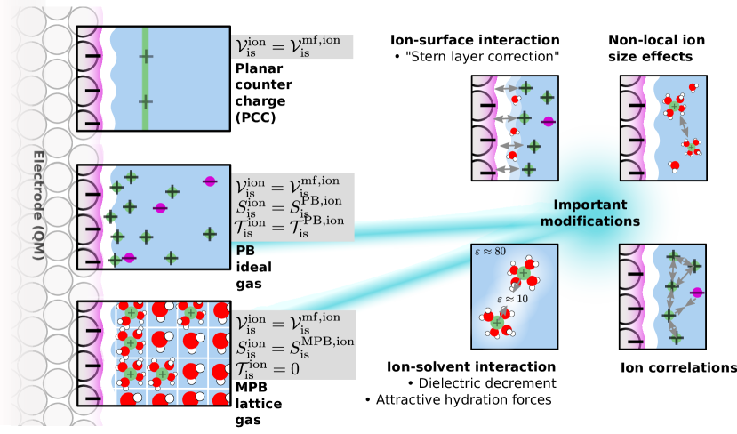
Figure 5: Schematic representation of various electrolyte models currently used for the description of SLIs. Planar counter charge (PCC) models place rigid ions in a Helmholtz layer like arrangement, while Poisson Boltzmann (PB) models determine the ionic distribution self-consistently in the total electrostatic potential. Various important modifications of PB theory are highlighted and discussed in the text.

As visualized in Fig. 5 such static ion distributions are indeed employed in so-called planar counter charge (PCC) models that are specifically developed for the description of planar SLIs¹⁷² and that we will further motivate in Section 2.5.6. However, for the general objective of deriving functional expressions for an electrolyte that is equilibrated in its response to the given electrode or solute with its (DFT) net charge density, it makes no sense to manually ascribe fixed ion positions. Indeed, the equilibrated ion density should be a result of the theory, and not an input. Therefore, this equilibrated density will have to adapt to the electrostatic potential, to which the ions though actually contribute themselves. This already shows that in such a case self-consistency between $\rho_{\rm ion}$ and $\phi$ in eq. (21) has to be reached. Most commonly, a corresponding self-consistent description of the ion distribution is achieved within the famous PB theory,^{113, 115, 114, 116} which treats the ions as a gas that interacts only via mean-field electrostatic interactions within the continuum dielectric. Referring to dedicated accounts on PB theory¹⁷³ for full derivations and a full appraisal, we here only compile the resulting expressions for the ion grand potential functional. For simplicity, we furthermore focus here and in the remainder of this electrolyte section also on an electrolyte with a cationic concentration $c_{+}=c_{+}({\boldsymbol{r}})$ due to only one cation species of mass $m_{+}$ and charge $+z$, and an anionic concentration $c_{-}=c_{-}({\boldsymbol{r}})$ due to only one anion species of mass $m_{-}$ and charge $-z$. Reflecting the additionally considered ion dynamics, the corresponding PB ion grand potential functional

$$\Omega_{\rm is}^{\rm ion}[\rho_{\mathrm{el}}]=\mathcal{T}_{\mathrm{is}}^{\mathrm{PB,ion}}[\rho_{\mathrm{el}}]+\mathcal{V}^{\mathrm{mf,ion}}_{\rm is}[\rho_{\mathrm{el}}]-TS_{\mathrm{is}}^{\mathrm{PB,ion}}[\rho_{\mathrm{el}}]\quad,$$ (22a)

now includes kinetic and, applying the famous Sackur-Tetrode equation,^{174, 175, 176} also entropic contributions. For the $$+z/-z$$ electrolyte they read

$$\mathcal{T}_{\mathrm{is}}^{\mathrm{PB,ion}}=\frac{3}{2}k_{\mathrm{B}}\int\left\{c_{+}+c_{-}\right\}\mathrm{d}\boldsymbol{r}$$ (22b)

$$S_{\mathrm{is}}^{\mathrm{PB,ion}}=-k_{\mathrm{B}}\int\biggl{\{}c_{+}\left[\ln\left(c_{+}\lambda_{+}^{3}\right)-\frac{5}{2}\right]+c_{-}\left[\ln\left(c_{-}\lambda_{-}^{3}\right)-\frac{5}{2}\right]\biggr{\}}\mathrm{d}\boldsymbol{r}\quad,$$ (22c)

with $\lambda_{\pm}=\frac{h}{\sqrt{2\pi m_{\pm}k_{\mathrm{B}}T}}$ the thermal wave length. The potential energy functional still holds as before in eq. (21), of course, now with the ion charge density given as $\rho_{\rm ion}=z(c_{+}-c_{-})$.

The starting point to obtain the self-consistent ion concentrations and electrostatic potential to evaluate these functional expressions is as before the GPE. Within the prevalent isotropic, linear and local dielectric model, and under the already mentioned assumption that the dielectric response of the solvent is not changed by the ion density, the electrolyte charge distribution can straightforwardly be added to the GPE of eq. (9), simply by extending the source terms on the right hand side

$$-\varepsilon_{0}\nabla\left[\varepsilon({\boldsymbol{r}})\nabla\phi\right] =(\rho_{\mathrm{el}}+\rho_{\mathrm{nuc}}+\rho_{\mathrm{ion}})\quad.$$ (23)

PB theory then additionally makes the assumption that in the equilibrated electrolyte the ions are Boltzmann-distributed in the electrostatic potential

$$c_{\pm}=c_{\infty,{\rm ion}}\exp\left(\mp\frac{z\phi}{k_{\mathrm{B}}T}\right)\quad,$$ (24)

with $c_{\infty,{\rm ion}}$ the constant equal concentration of cations and anions in the bulk of the electrolyte. Within the mean-field PB gas ansatz, $c_{\infty,{\rm ion}}$ is in turn readily related to the bulk ion electrochemical potential via $\tilde{\mu}_{\mathrm{ion},\pm}=k_{\mathrm{B}}T\ln\left(\lambda_{\pm}^{3}c_{\infty,{\rm ion}}\right)$. Inserting eq. (24) into the ion-including GPE of eq. (23), leads finally to the famous PB equation (PBE) itself

$$\varepsilon_{0}\nabla\left[\varepsilon\nabla\phi\right]=-\left(\rho_{\mathrm{el}}+\rho_{\mathrm{nuc}}+2zc_{\infty,{\rm ion}}\sinh\left(-\frac{z\phi[\rho_{\mathrm{el}}(\boldsymbol{r})]}{k_{\mathrm{B}}T}\right)\right)\quad,$$ (25)

which does not explicitly contain the spatially varying ionic concentrations anymore. In practice, this PBE can thus be implemented into the KS-DFT minimization in a way completely analogous to the GPE of the ion-free case, and then be solved at each electron density optimization step. However, due to the complicated non-linear nature of the PBE, and the associated computational cost of solving it, it is popular to instead solve a simplified linearized version of it.^{177, 178} This linearized Poisson-Boltzmann equation (LPBE) can be obtained by truncating a Taylor expansion of the sinh-term in eq. (25) around $\phi=0$ (here assumed to be the bulk electrolyte potential) after the linear term¹¹⁶

$$\varepsilon_{0}\nabla\left[\varepsilon\nabla\phi\right]=-\left(\rho_{\mathrm{el}}+\rho_{\mathrm{nuc}}-\frac{2z^{2}c_{\infty,{\rm ion}}}{k_{\mathrm{B}}T}\phi[\rho_{\mathrm{el}}(\boldsymbol{r})]\right)\quad.$$ (26)

The corresponding LPBE grand potential functional terms can then be derived analogously from a Taylor expansion of eq. (22).¹³⁰

As mentioned at the beginning of this sub-section, the assumptions underlying PB theory restrict its formal range of applicability to dilute electrolytes. Close to electrified SLIs, however, high ion concentrations may accumulate even for electrolytes that are indeed dilute in the bulk.^{117, 179} This motivates corrections to PB theory that account for then increased ion-ion and ion-solvent correlations. Despite the non-locality of these interactions, a series of local ion density approximation models have been proposed to keep the simplicity of the PB model intact. They are summarized in Fig. 5 above and will be briefly outlined in the following.

2.5.2 Finite ion size corrections

In the original formulation of PB theory, ions are point-like. This means, that for stronger fields local ion concentrations could in principle reach unphysically high values. An immediate fix to this problem is to simply give ions a finite size, which then leads to size-modified PB (MPB) theory.¹⁸⁰ While MPB can be derived in various ways,¹⁸¹ the most physically intuitive derivation is based on a lattice model with a uniform cell size $a$ for (solvated) ions and solvent molecules, where each lattice site can at max hold only one particle, cf. Fig. 5. This way, the lattice mimics short-range ion-ion repulsion and by construction does not allow unphysically high local ion concentrations. For this model, an ion grand potential functional can be developed using the configurational partition function of solvent molecules and ions, and then applying a mean-field approximation.^{182, 117, 183, 132} The model thus corrects in a mean-field way for ion repulsions, and the kinetic energy and entropy functionals are modified as

$$\mathcal{T}_{\mathrm{is}}^{\mathrm{MPB,ion}}=0$$ (27)

$$S_{\mathrm{is}}^{\mathrm{MPB,ion}}=-k_{\mathrm{B}}\int\biggl{\{}c_{+}\left[\ln\left(c_{+}a^{3}\right)-1\right]+c_{-}\left[\ln\left(c_{-}a^{3}\right)-1\right]$$

$$\quad\quad\quad\quad+\left(\frac{1}{a^{3}}-c_{+}-c_{-}\right)\ln\left(1-c_{+}a^{3}-c_{-}a^{3}\right)+c_{+}+c_{-}\biggr{\}}\mathrm{d}\boldsymbol{r}\quad.$$ (28)

The ion concentrations now effectively follow a Fermi-Dirac-like statistics due to the maximum occupancy of the lattice cells

$$c_{\pm}=c_{\infty,{\rm ion}}\frac{\exp\left(\mp\frac{z\phi}{k_{\mathrm{B}}T}\right)}{1-2c_{\infty,{\rm ion}}a^{3}+2c_{\infty,{\rm ion}}a^{3}\cosh\left(\frac{z\phi}{k_{\mathrm{B}}T}\right)}\quad,$$ (29)

with the relation between the bulk concentration and ion electrochemical potential modified to $\tilde{\mu}_{\mathrm{ion},\pm}=k_{\mathrm{B}}T\ln\left(\frac{c_{\infty,{\rm ion}}a^{3}}{1-2c_{\infty,{\rm ion}}a^{3}}\right)$. In direct analogy to the unmodified PB case, inserting these concentrations into the GPE of eq. (23) leads then to the so-called MPB equation, which in turn gives the desired functional relation between electrostatic potential and electron density and which can be solved within the KS DFT minimization as before.

The MPB ion concentration profiles converge to the PB profiles for $a\rightarrow 0$, if the same bulk electrochemical potential reference is used. One can easily see that this then implies $a=\lambda_{+}=\lambda_{-}$, i.e. within PB theory the thermal wavelength plays the same role as the ion size in MPB theory. The two theories thus have a common algebraic origin, but a different physical one. Indeed, in contrast to PB theory and as seen in eq. (27), the MPB model lacks an ion kinetic energy functional. Yet, since it equally lacks a corresponding entropy contribution from the ionic motion and with the two terms canceling each other in PB theory, the same functional form is nevertheless recovered in both theories for the small ion size limit. Note also that the original MPB theory, and the corresponding equations above, were developed for equally sized cations and anions. It has since been extended to asymmetric electrolytes, e.g. by extending the statistical lattice model with sublattices,^{184, 185} by introducing potential-dependent ion sizes¹⁸⁶, or by other means.^{187, 188} There are also efforts to go beyond the lattice approximation,¹⁸⁹ deriving functional expressions from experimental equation of state data or from equations defining atomic or molecular interactions such as closure relations to the Ornstein-Zernicke equation, cf. Section 2.1.^{190, 188} Notwithstanding, the resulting energy functionals are generally still based on a local approximation for the ion density. Such local approaches to ion-ion interactions offer generally a simple correction to PB theory for those situations where ions are crowded, e.g. due to strong electric fields. However, in case of strong variations of the ion concentration profiles the description of $\Omega_{\rm is}^{\rm ion}[\rho_{\rm el}]$ as a local functional of ion concentrations may break down altogether. Such cases may then necessitate a more involved non-local treatment.¹⁹⁰

2.5.3 Ion-induced solvent structuring

One important physical effect of the ions completely omitted so far is simply the fact that in regions with high ion concentrations few solvent molecules may reside, and if they do they are likely highly structured around the ions. In such situations the dielectric continuum approximation for the solvent likely breaks down and ion interactions become much more specific than the the hitherto included mean-field electrostatics.

Accounting for this effect, Burak and Andelman¹⁹¹ derived a corrective short-range ionic interaction potential contribution to the mean-field electrostatic potential from Monte Carlo simulations. By truncating the virial expansion of the PB partition function after second order, they were then able to derive a simple analytic expression for the free energy. Although this direct expansion approach is of great interest for the development of improved PB-based theories, it is less practical due to the required knowledge of the system-dependent fluctuating short-range potential. An approach that is in this respect more in the spirit of effective parametrized continuum models has been put forward by Bohinc, Shrestha and May.^{192, 193, 194} There, they represented the additional short-range forces by a parametrized Yukawa potential, arriving at a simple correction to PB theory. Next to this, several other approaches have been developed in the past for which we refer the interested reader to an extensive review on this topic.¹⁹⁵

All of the above corrections share the fact that the resulting corrections are non-local in the sense that solvent structure at a point in space is also influenced by the ion concentration in its vicinity (e.g. via the aforementioned short-range potentials). A much simpler and local variant to correct for ion-induced solvent structuring is the dielectric decrement approach, cf. Fig. 5. From simulations¹⁹⁶ and various experimental works,^{197, 198, 199, 200} it has been found that the isotropic dielectric permittivity of water varies linearly with the salt concentration at small to medium (1.5 M) salt concentrations,²⁰¹

$$\varepsilon_{\infty}(c_{\infty,{\rm ion}})=\varepsilon_{\infty}(c_{\infty,{\rm ion}}=0)+\beta c_{\infty,{\rm ion}}\quad,$$ (30)

where $\beta$ is a generally negative, ion-specific dielectric decrement coefficient indicating how easy the water structure can be polarized by the presence of salt. The equation can be also written as a function of the local salt concentration, but importantly anionic and cationic contributions cannot be separated without making further assumptions, due to a lack of experimental data.²⁰¹ In any case, based on this evidence for water one could simply consider $\beta$ as a further variable parameter and modify the dielectric function employed for the mean-field electrostatics, cf. Section 2.3.2, to additionally depend (linearly) on the local ion concentration. In the SLI context with aqueous electrolytes, this effective dielectric decrement approach also enjoys recent popularity to model a stronger (sometimes ice-like) water structuring in the inner DL through an accordingly reduced dielectric permittivity in that region.²⁰² In summary, there are thus a number of methods of varying degrees of complexity that allow to mimic an ion-induced local structuring of the solvent around a solute. Thereby, they extend the validity of PB or MPB approaches to higher ion concentrations, yet often at the price of additional parameters that need to be determined.

2.5.4 Coulombic ion correlations

In the case of small ion concentrations with thus effectively large ion separations and in strongly screening solvents like water, the mean-field interaction between the dissolved ions assumed in PB theory is generally a good approximation. However, it may quickly break down for solvents with smaller dielectric permittivity, for higher ion concentrations (such as in ionic liquids^{203, 204}), or for multi-valent ions with stronger Coulomb forces.^{191, 186, 205} In these cases, the electrostatic force is much more non-local and fluctuating, leading for example to the effect of overscreening at charged interfaces.²⁰⁶ Overscreening in the context of electrified SLIs refers to the presence of higher amounts of counter charge in the electrolyte close to the electrode than needed to compensate the surface charge, followed by a smaller net charge of opposite sign to satisfy overall electroneutrality.

An account for the corresponding ion correlations requires in general field theoretical approaches, using loop expansions, which lead to substantially more complicated expressions than in PB theory.^{207, 208} A promising, more approximate approach by Bazant et al. instead leads to a simple correction of the mean-field electrostatic potential energy, cf. eq. (21), in form of one added term²⁰⁵

$$\mathcal{V}_{\rm is}^{\mathrm{non-mf,ion}}[\rho_{\mathrm{el}},\phi]=-\int\frac{\varepsilon_{0}\varepsilon({\bf r})}{2}l_{c}^{2}(\boldsymbol{\nabla}^{2}\phi)^{2}\mathrm{d}\boldsymbol{r}\quad,$$ (31)

where the parameter $l_{c}$ represents an electrostatic correlation length. This demonstrates nicely that the electrostatic energy is lowered due to overscreening by enhancing the curvature of $\phi$. The theory was shown to give overscreened ion distribution profiles in close agreement with molecular dynamics simulations resulting in realistic estimates of the potential-dependent capacitance compared to experimental reference data.²⁰⁵

2.5.5 Ion-solute interaction and Stern layer formation

PB and MPB theories as well as their extensions are usually derived without the actual presence of the solute. Therefore, the only coupling between solute and ions is the hitherto discussed mean-field electrostatic coupling. Just as highlighted in Section 2.4 for the pure liquid, this neglects additional interactions between the ions and the solute that were for the solvent summarized in the $\Omega_{\mathrm{is}}^{\mathrm{non-el}}[\rho_{\mathrm{el}}]$ term in eq. (2). A prominent such non-electrostatic correction for the ions would be an additional repulsive contribution which prevents ions to approach the solute too closely. In protic solvents, the formation of a corresponding ion-free solvent region called Stern layer is for instance a consequence of the large size of the hydrated cations.

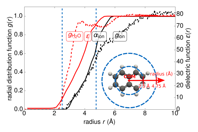
Figure 6: Creation of an ion-free Stern layer around a molecular solute. Compared is the solvation environment around the center of mass (COM) of naphthalene in a 2.18M NaCl solution as obtained from explicit molecular dynamics simulations ²⁰⁹ (dashed lines) and with a Stern-layer corrected implicit MPB model (solid lines). Data in red represents the spherically-averaged radial distribution function (RDF) of the oxygen atoms in the explicit water solvent ($g_{\rm H_{2}O}$) and the corresponding spherically-averaged dielectric function $\varepsilon$ for the implicit model. Data in black are the spherically-averaged RDF for the ions and the corresponding ion-exclusion function $\alpha_{\rm ion}$. Both the onset of the solute solvation shell and the radial Stern layer shift of the ionic distribution are rather well reproduced. To better grasp the involved scales, two dotted vertical lines illustrate the radial distance to the molecule COM as shown in the top view in the inset. Adapted with permission from ref. 120, American Institute of Physics (AIP).

Most straightforwardly, this kind of physics can be implemented by an additional repulsion potential added on top of the mean-field potential. Alternatively, the repulsion potential can simply be expressed as an exclusion function $\alpha_{\mathrm{ion},\pm}=e^{-\frac{\phi^{\mathrm{rep}}_{\pm}}{k_{\mathrm{B}}T}}$ for cations and anions, respectively. The exclusion function prevents the ions from approaching the solute to a certain distance,¹³² similar to the dielectric shape function controlling the solvent’s place of closest approach (see ref.132 for a full derivation following the statistical lattice approach). This leads to a modified set of ion concentration functions, which for the case of a +z/-z electrolyte read

$$c_{\pm}=c_{\infty,{\rm ion}}\alpha_{\mathrm{ion},\pm}[\rho_{\mathrm{el}}]\frac{\exp\left(\mp\frac{z\phi}{k_{\mathrm{B}}T}\right)}{1-2c_{\infty,{\rm ion}}a^{3}+2c_{\infty,{\rm ion}}a^{3}\alpha_{\mathrm{ion},\pm}[\rho_{\mathrm{el}}]\cosh\left(\frac{z\phi}{k_{\mathrm{B}}T}\right)}\quad.$$ (32)

For the sake of convenience the functional form for $\alpha_{\mathrm{ion},\pm}$ can be chosen identical to the dielectric shape function $s_{\rho_{\mathrm{el}}}$, to vary in between 0 in the ion-free region and 1 in the ion-contained electrolyte region, yet with a different cutoff parameter that can be individually tuned.¹²⁰ This simplified model was shown to be able to account for short ranged ion-solute interactions, at the price of the additional cutoff and shape parameters. As detailed in Section 2.6, a careful tuning of these parameters to reproduce molecular experimental reference data yields a plot like in Fig. 6, which nicely illustrates the achieved creation of an ion-free Stern layer close to the solute with an extent and location that agrees well with the results of molecular dynamics simulations with explicit solvent. Below, we will refer to a MPB model that additionally provides such a Stern-layer functionality as S-MPB model.

2.5.6 Planar counter charge models

All the ion models presented so far are based on diffuse layer theory, essentially assuming mobile gas like ions that migrate and equilibrate in a mean-field potential. While these more physical approaches are most valuable for a general treatment of solvation, the aforementioned, much simpler PCC approach to place rigid ions into the supercell, cf. Fig. 5, is of particular interest and convenience for the context of planar SLIs. As further discussed in Section 3.4 below, its primary purpose is to introduce a counter charge distribution that exactly compensates a net charge of the electrode to achieve an overall charge-neutral supercell. As the name says, this ionic counter charge distribution is simply modeled as a smoothed out Gaussian charge plane.¹⁷² The advantage of this method is that the ionic charges can be freely shifted in space, thereby providing some flexibility, e.g. in modeling asymmetric DFT supercells with only one slab side exposed to the electrolyte. Physically, the PCC model resembles if at all the situation in the inner DL, where the ions are assumed to be highly crowded. In dominantly studied aqueous electrolytes, the obvious crudeness of this approach is fortunately to some extent remedied by the strong screening capabilities of the polar solvent, which renders the DL potential drop less sensitive to the exact location of the ions.

2.6 Parametrization

As apparent from the presentation so far, implicit solvation methodologies come invariably with a set of (in principle system-dependent) parameters, and it is these parameters that crucially determine the accuracy of this highly effective approach to solvation. To recap the previous sections, parameters arise generally in the functional expressions accounting for electrostatic, non-electrostatic and ionic contributions. In the standard linear, local and isotropic dielectric formulation of the electrostatic contribution, parameters are needed to define the location of the solvation cavity, or additionally the dielectric transition region. As discussed in Section 2.3.2, these can be atomic radii in the case of spatially parametrized dielectric functions, or iso-values of the electron density in the density-dependent case. The non-electrostatic energy functional also gives rise to a varying number of parameters that depends strongly on the models of choice. If the models separately account for cavitation, dispersion or repulsion, quite a large number of parameters can quickly arise. In contrast, the simplified SCCS model of Andreussi et al.¹²⁹ lumps all of this into just two parameters that scale the solvation cavity volume and surface. Lastly, the ionic energy functional comes with its own number of parameters to express deviations from the PB theoretical description. These can either be the introduction of a finite ion size parameter, a parameter to describe the Stern layer and thus solute-ion interactions, or parameters to describe ion-solvent interactions in form of a dielectric decrement.

Depending on the model complexity and the way it considers these various contributions, a largely different total number of parameters can result. This number can range from just four in the minimal SCCS model¹²⁹ to 64 parameters in the popular SMD model.²¹⁰ These parameters may then be determined to give an optimum account of maybe only a single solvent/solute combination, maybe a particular solvent (e.g. water in the case of the SCCS model), or aiming at maximum transferability for a whole range of solvents (as in the SMD case). At the same time, due to the fitting procedure, there is always the possibility of some degree of error cancellation, when for instance the non-electrostatic contributions compensate for some of the shortcomings of the DFT functional itself.¹³¹ A key question is thus, to which degree the use of parameters can improve the physics and transferability of the implicit solvation model. This question relates directly to the size, quality and information content of the available training data to which parameters can be fitted.

In principle, training data should be selected that is as close as possible to the intended application, in this case SLIs, or if possible even electrified SLIs. Unfortunately and as further discussed in Chapter 3, experimental reference data is very rarely available for these systems, and if it is, it is often not suited for the parametrization of a microscopic solvation model. The main reason for this is that at SLIs various other effects overlap with pure solvation contributions as we will see in the next chapter below. In contrast, molecular solvation data is much more widely available, at least for water as a solvent. Therefore, many implicit solvation studies on SLIs have adapted parameters that have originally been derived from a parametrization to such molecular data. This is not only critical from the viewpoint of the largely different chemistries, involving solutes composed of light organic elements in one case and extended electrodes composed of heavy transition metals in the other. There are also practical problems that arise not least from the different dimensionality of the problem. For instance and as outlined in Section 2.4.2 above, non-electrostatic contributions can be expressed as a function of the volume of the solvation cavity, which in turn is not defined for extended interfaces. Such issues have led to the formulation of functional expressions that only involve quantities compatible with SLIs. In the mentioned example, this is a non-electrostatic model that only considers the cavity surface and not the volume.^{129, 131} Nevertheless, also such models are then re-parametrized using the existing molecular databases. The performance of the cavity-surface model was there found to be similar to the original one including the cavity volume. While this suggests that a parametrization of SLI-compatible models is possible, it still does not tell how well the molecular parameters will transfer to the SLI context and we will come back to this issue in the next chapter.

Database	# Solvents	# Solutes	# Hydration	# NAQ solv.
			energies	energies
FreeSolv (v0.51)211	1 (W)	643N	643	0
Wang212	1 (W)	668N	668	0
Rizzo-DGHYD213	1 (W)	538N/52C	603	0
Kelly214	1 (W)	106C	106	0
MNSol (v2.0)215	106 (W,NAQ)	662N	389	2648
Solv@TUM (v1.0)216, 119, 217	145 (NAQ)	658N	0	5952
CompSol218	732 (W,NAQ,IL,T)	863N	397 (581*)	3786 (13386*)

Table 1: Databases containing experimentally measured solvation energies of molecular solutes at room temperature. C = charged, N = neutral, W = water, NAQ = no-aqueous solvents, IL = ionic liquids, T = temperature dependence. The numbers were extracted from the respective databases directly. The Wang database is to a large part constructed from the FreeSolv database. *Only solvation energies evaluated at $25\pm 2^{\circ}$C have been considered, while the number in brackets refers to the complete number of solvent-solute combinations for which at least one temperature data is available.

If one accepts that the parametrization is done with molecular data, the next obvious questions are which and how much of such data is available, how diverse the database is in terms of a wide range of molecular chemistries and whether the tabulated quantities are in fact really suited for the parametrization at hand. In the long, independent history of molecular solvation modeling, these questions have been satisfactorily addressed through the built-up of databases of primarily experimental solvation free energies. As apparent from Table 1, these databases are indeed sizable and partly contain data for a wide variety of solvents. Out of these, the Minnesota solvation (MNSol) database²¹⁵ was among the first to provide experimental solvation energies of a wide range of over 600 neutral organic molecules in over 100 different solvents. Over the years, this database has been extended and various other databases have appeared. The FreeSolv²¹¹ database is currently the largest collection of neutral molecule solvation free energies in water (then called hydration energies). It consists of over 600 entries and should thus allow a meaningful parametrization even of more complex models.

Within the implicit solvation framework defined in this review, a molecular solvation free energy is calculated as

$$\Delta G_{\mathrm{solv}}=\Omega^{N_{\alpha}}_{\varepsilon_{\infty}={\rm solv}}[\rho_{\mathrm{el}}^{\circ}]-\Omega^{N_{\alpha}}_{\varepsilon_{\infty}=1}[\rho_{\mathrm{el}}^{\circ}]\quad,$$ (33)

where the two grand potential terms correspond to the solute in the solvent and the solute in vacuum, at their respective (generally different) ground state electronic densities $\rho_{\mathrm{el}}^{\circ}$. Note that it is awkward to see a free energy on the left hand side of the equation, and a difference of grand potential energies on the right hand side. We here simply attest to the fact that (measurable) solvation free energies are generally seen as a property of the full (macroscopic) system and not of the grand-canonical sub-system technically employed in the calculations. Starting our survey of model performance with the ubiquitous solvent water, implicit solvation models trained by these molecular databases can typically predict hydration energies with a mean absolute error (MAE) between 0.6 kcal/mol (large parameter space models like SMD²¹⁰ or SM8¹³³) up to 1.2 kcal/mol (small parameter space models like the SCCS model¹²⁹). In general, though, these numbers are difficult to compare, since rarely the same set of training and test molecules have been used, see e.g. ref.219 for a notable exception. Nevertheless, it generally seems that standard implicit solvation models have had a hard time to decrease the accuracy below about  0.5 kcal/mol, which could thus somehow mark what can realistically be expected at such high level of coarse graining. Recent reports of ground-breaking 0.14 kcal/mol MAEs²²⁰ with new machine-learned implicit solvation models have thus also to be seen in light of the actual accuracy of the underlying experimental data. Different solvation databases have been found to have an error of up to 0.25 kcal/mol relative to each other,^{119, 218} which agrees with the experimental error that is estimated for solvation energies of neutral solutes based on measured partition coefficients.^{119, 221} Too highly parametrized models could therefore run the risk of overfitting of experimental errors. A connected problem is the occurrence of solutes in the training set which are reactive in solution. The optimized SCCS model was, for example, found to perform well for most molecular components, apart from carbonic acids and amines. These are precisely those compounds which are mostly present in solution in their dissociated form at associated vastly different solvation energy. This highlights the importance of a careful curation of the reference databases.

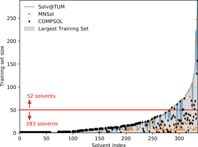
Figure 7: Number of solvation energy entries (“training set size”) per non-aqueous solvent in the three largest corresponding experimental databases. The solvents are sorted according to their largest training set size in all of the three databases. Training set sizes below 50 are prone to significant overfitting errors, in particular if the solutes are not homogeneously distributed over the chemical space.

Next to the simulation of aqueous solvation, also non-aqueous solvents are of high importance for electrochemistry, such as e.g. for lithium ion batteries²²² or the electrocatalytic reduction of CO₂.²²³ As shown in Table 1, the Solv@TUM database^{216, 119, 217} currently has the largest total collection of non-aqueous solvation energies of neutral organic molecules, but this does not tell how large a training set is available for each individual non-aqueous solvent. Figure 7 correspondingly compares the MNSol, Solv@TUM and COMPSOL databases regarding this amount of available solvation energies for each non-aqueous solvent. It is apparent that for most of these solvents the databases actually contain less than 50 solvation free energy entries. As pointed out by Hille et al.,¹¹⁹ such small training set sizes for the implicit solvation model can result in significant overfitting of the data. This would likely reduce the transferability even for those implicit solvation models that have only a few fitting parameters. Unfortunately, the situation is even worsened by an often low chemical diversity of the organic solutes contained in these small test sets, which may further lead to bias in the achieved parametrization.¹¹⁹ These issues provide a motivation especially for smallest parameter space implicit solvation models that rather trade quantitative accuracy with a somewhat robust extrapolation outside of the small training regime. As we will elaborate further in Chapter 3 below, this objective fits actually very well with the realization that the primary value of implicit solvation modeling at SLIs is presently more the provision of a counter-charge model than the actual account of solvation effects. Within this perspective, a recent reformulation was able to reduce the parameter space of the SCCS model to a single non-electrostatic parameter, while still resulting in a reasonably accurate prediction of solvation free energies for most solvents.¹¹⁹ This one parameter can furthermore be estimated from the solvent bulk dielectric permittivity, enabling the prediction of solvation free energies for arbitrary solvents with known permittivity.

The problem of small training set sizes becomes even more critical when transitioning to solvation free energies of charged solutes. Estimating the solvation energy of ions is a key challenge of high priority, as charged systems appear constantly as reactants or reaction intermediates in electrochemistry,²²⁴ but also e.g. in bio-²²⁵ or organic chemistry.²²⁶ The solvation energy of dissociated acids for example is important for the estimation of the acid dissociation constant,²²⁷ or the solvation energy of charged redox species for the calculation of redox potentials.²²⁸ Due to their large electrostatic stabilization, charged solutes exhibit solvation energies that are an order of magnitude larger than the ones of neutral solutes. However, the experimental measurement of single molecule ionic solvation energies requires thermodynamic cycles and the knowledge of the absolute solvation free energy of an arbitrary reference ion, usually a proton.^{229, 230, 214} Especially, the latter has been found to be prone to errors up to 2 kcal/mol.²¹⁴ Nevertheless, various attempts have been made to parameterize implicit solvation models to ionic solvation data, as e.g. the Rizzo-DGHYD database²¹³ containing 52 solvation energies of cations and anions. In using this database for parametrizing the SCCS model, Dupont et al. found substantially different cavity parameters for anions, cations and neutral molecules,¹³⁹ which one would generally avoid for the modeling of SLIs with a varying charge state depending on the applied potential. This issue may be due to two drawbacks of the original SCCS approach. First, relying on the electron density to define the dielectric function, cf. Section 2.3.2, means that anions show significantly larger cavities compared to cations and neutral molecules at comparable density iso-values.^{135, 131} Furthermore, SCCS does not account for explicit solvent-solute correlation, which becomes significant in the case of high fields near localized charges. As noted above, electric field corrected dielectric functions have shown promise to go beyond this limitation.^{138, 140}

Next, in an attempt to increase the training data for implicit solvation models, the CompSol database has recently been published adding further quantities beyond the traditional solvation free energies at standard state. These are mainly temperature-dependent solvation free energies and solvation energies in ionic liquids. In terms of solvation energy entries, this database is now by far the largest. In order to make full use of it though, the implicit solvation model actually has to be able to somehow account for the additional physics in this data. Indeed, temperature-dependent solvation data could provide an additional constraint on the functional form of electrostatic, cavity or dispersion energy contributions, all of which could in principle depend on the temperature.^{231, 232, 233} While some implicit solvation models incorporating temperature effects have been communicated,²³⁴ these have not found their way into widespread use to date.

As a final point, we note that all of the databases discussed above focus on solvation free energies for vanishing ionic concentrations in the solvent. They are thus not suited for the determination of the ionic parameters appearing in electrolyte models that go beyond the plain PB approach. Ionic parameters suffer therefore presently from the highest scarcity of reference data. One remedy is to realize that finite salt concentrations are known to alter the solvation free energy of neutral solutes in aqueous solution nearly linearly. This is described by the so-called Setchenow equation^{235, 236}

$$\Delta G_{\rm solv}(c_{\infty,{\rm ion}})-\Delta G_{\rm solv}(0)=k_{\mathrm{s}}\frac{k_{\mathrm{B}}T}{\log_{10}(\mathrm{e})}c_{\infty,\mathrm{ion}}\quad,$$ (34)

with the Setchenow coefficient $k_{\mathrm{s}}$ and $e$ the electronic charge as a positive value. From tabulated Setchenow coefficients, one can estimate that a 1 M ion concentration in the electrolyte decreases solvation free energies by 0.1-0.3 kcal/mol, where the dominating effect is the energy penalty to create the ionic cavity.¹²⁰ Such apparently small changes to the solvation free energies can still have critical consequences, at least if one thinks of biochemistry where they are known to induce protein folding. Accounting for these changes may also be key in fitting implicit models to experimental solvation data with possibly finite salt concentrations. In this respect, tabulated Setchenow coefficients actually represent a direct way to determine the ionic parameters of the implicit solvation model. Ringe et al. used such a database of experimentally tabulated Setchenow coefficients to optimize the electron density cutoff that controls the ionic cutoff function $\alpha_{\mathrm{ion}}^{\pm}$ using an SCCS/S-MPB model.¹²⁰ This density cutoff was found to be correlated with the hydration number of the ions in the solution, showing that the parametrized model was able to predict ion-specific hydration effects for neutral molecules.

To recapitulate, most contemporary implicit solvation models applied to the simulation of SLIs tend to use parameters derived from molecular solvation databases as a basis. While the actual transferability of these parameters to the SLI context is still unclear, there is generally at least sufficient molecular experimental reference data available to achieve a coherent parametrization for water as a predominant solvent also in interfacial electrocatalysis applications. The situation worsens quickly for non-aqueous solvents and is critical for ionic parameters. While this sets a perspective for the complexity of implicit solvation modeling one can aspire to, it clearly shows that even in the context of molecular solvation there is still room for improvement through the establishment of larger and chemically more diverse reference data bases including entries beyond standard state solvation free energies.

2.7 Implicit solvation implementations in DFT program packages

As we have shown in the previous sections, a wide variety of implicit solvation methodologies exist and it is their recent implementation into DFT program packages that can also deal with extended surfaces (e.g. through the use of periodic boundary condition supercells) that has enabled such kind of modeling for the SLI context at all.

Table 2 shows a compilation of the implicit solvation methods and features that have been implemented into various state-of-the-art, periodic and non-periodic DFT program packages at the time of submission of this article. It clearly shows a tendency of predominant use of local, linear and isotropic dielectric models. All-electron DFT packages traditionally use sharp apparent surface charge (ASC) models, cf. Section 2.3.2, instead of smooth dielectric models. This is partly due their logarithmic integration grid structure to resolve localized core basis functions, which makes the solution of the GPE or PBE over the whole computational domain numerically difficult. ASC models have been implemented also in connection with the LPB equation to simulate simplified SLIs.²³⁷ Among all these realizations of implicit solvation models, FHI-aims has been the first all-electron DFT package implementing a smooth dielectric response model (SCCS¹²⁹), extended by an advanced Stern-layer and ionic size (lattice model) corrected PB (S-MPB) ion representation.^{130, 120, 132} It also introduced an efficient Newton solver linearizing the S-MPB equation¹³⁰, which has recently also been adapted by other DFT packages.²⁵ Q-Chem is an interesting alternative, in particular for non-equilibrium (frequency-dependent dielectric function) solvation calulations or heterogeneously structured dielectrica (e.g. solvation at vacuum-water or liquid-liquid interfaces) via ASC methods. Q-Chem has also recently implemented the smooth dielectric S-MPB model to support modeling of electrolytes.²³⁸

The so far discussed program packages are ideal for the simulation of electrochemistry of finite-size nanoparticles. The implicit solvation simulation of extended metallic electrodes, realized by supercells with periodic boundary conditions, has been made available in several ASC schemes, implemented in CRYSTAL,²³⁹ GAUSSIAN²⁴⁰ and Dmol³.²⁴¹ However, this domain is clearly dominated by pseudo-potential and then mostly plane-wave based DFT program packages, with their efficient Fourier-transform algorithms for periodic systems. Here, QUANTUM ESPRESSO¹⁷² and JDFTx²¹ are presently the clear leaders with most advanced implementations of solvation and ion models. In addition, QUANTUM ESPRESSO provides most sophisticated correction schemes for removing periodic boundary condition in the normal direction of the surface slab to avoid artificial slab-slab interactions.^{242, 243} VASP, arguably the most popular DFT code in the theoretical electrochemistry community, provides so far only basic implicit solvation functionality, but at least also a LPB solver which provides counter charges and then allows simulations of charged interfaces.¹⁷⁸ As pointed out in recent works, the use of VASP requires special care though due to the not self-explanatory shifting of the electrostatic potential and also problems with the dipolar slab correction which is supposed to correct slab-slab interactions across periodic boundaries.^{244, 245, 24} Other packages, such as GPAW,²⁰² ONETEP²⁴⁶ and BIGDFT²⁴⁷ have recently also reported the required implementations for S-MPB based implicit solvation models and should thus also be valid options for future modeling of electrified interfaces.

		Dielectric model ($\varepsilon$)
		Lin. model/		Non-lin.	Het.
DFT package	BCs	Shape $s$	Non-loc	Aniso	Non-eq.	Salt model
—full potential / all-electron—
		$s_{\rho_{\mathrm{el}}}$/$s_{\boldsymbol{r}}$,135, 238		$\times$	$\checkmark$248, 249	S-MPB238,
		$s_{\rho_{\mathrm{el}}}$250/$s_{\boldsymbol{r}}$			$\checkmark$251, 252, 253, 254, 255	LPB
					256, 253, 48
Q-Chem257	F	(ASC258)	$\times$	$\times$	259, 248, 249	(ASC260)
		$s_{\rho_{\mathrm{el}}}$129, 130,		$\times$	$\times$	S-MPB
FHI-aims261	F	$s_{\rho_{\mathrm{el}}}$(ASC131)	$\times$	$\times$	$\times$	130, 120, 132
		$s_{\boldsymbol{r}}$		$\times$	$\times$
CRYSTAL262, 263	P239/F	(ASC239, 264)	$\times$	$\times$	$\times$	$\times$
		$s_{\boldsymbol{r}}$		$\times$	$\times$	LPB
Jaguar265	F	(ASC266, 267, 268, 133, 269)	$\times$	$\times$	$\times$	(ASC266, 267, 268)
		$s_{\rho_{\mathrm{el}}}$/$s_{\boldsymbol{r}}$		$\times$	$\checkmark$270	LPB
GAMESS271	F	(ASC28)	$\times$	$\checkmark$237, 272, 273	$\checkmark$274, 275, 276, 277	(ASC278)
		$s_{\rho_{\mathrm{el}}}$/$s_{\boldsymbol{r}}$		$\times$	$\times$	LPB
GAUSSIAN279	P240/F	(ASC28)	$\times$	$\checkmark$280	$\checkmark$281, 282, 252, 283, 256	(ASC278)
		$s_{\boldsymbol{r}}$		$\times$	$\times$
Dmol3	P241/F	(ASC134, 241)	$\times$	$\times$	$\times$	$\times$
		$s_{\rho_{\mathrm{el}}}$/$s_{\boldsymbol{r}}$		$\times$	$\times$
TURBOMOLE284	F	(ASC134, 285, 286)	$\times$	$\times$	$\checkmark$287, 283	$\times$
				$\times$	$\times$
NWChem288	F	ASC134, 289	$\times$	$\times$	$\times$	$\times$
—pseudopotential—
		$s_{\rho_{\mathrm{el}}}$290, 137		$\times$	$\times$
VASP291	P		$\times$	$\times$	$\times$	LPB178
		$s_{\boldsymbol{r}}$135, 127,		$\times$	$\times$	LPB, S-MPB,
QE292, 293, 294, 295	P/F	$s_{\rho_{\mathrm{el}}}$129	$\checkmark$127	$\checkmark$	$\times$	PCC247, 25
		$s_{\boldsymbol{r}}$135		$\times$	$\times$
BigDFT296, 297, 298, 299, 300	F/P301	$s_{\rho_{\mathrm{el}}}$129	$\times$	$\times$	$\times$	MPB247
	P/	$s_{\boldsymbol{r}}$,302		$\times$	$\times$	DD-S-MPB,
GPAW303, 304	F302, 305, 202	$s_{\rho_{\mathrm{el}}}$,129, 136	$\times$	$\times$	$\times$	LPB, PCC202
				$\times$	$\times$
PWMat306, 307	P	$s_{\rho_{\mathrm{el}}}$129, 308	$\times$	$\times$	$\times$	S-LPB247, 308
		$s_{\boldsymbol{r}}$,135	$\checkmark$	$\checkmark$125, 22, 309		CS-MPB,125
		$s_{\rho_{\mathrm{el}}}$137, 125, 22, 126	310, 111, 138	111, 138	$\times$	S-CS-MPB,309
JDFTx311	P/F			$\checkmark$312	$\times$	LPB125, 313
		$s_{\rho_{\mathrm{el}}}$129, 136, 314		$\times$	$\times$
CP2K315	P		$\times$	$\times$	$\times$	$\times$
		$s_{\boldsymbol{r}}$,135, 316, 246		$\times$	✓a317	S-MPB246
ONETEP318	P/F317	$s_{\rho_{\mathrm{el}}}$319, 136, 316, 246	$\times$	$\times$	$\times$	320, 321, 316, 246
				$\times$	$\times$
CASTEP322	F	$s_{\rho_{\mathrm{el}}}$136, 316, 246	$\times$	$\times$	$\times$	$\times$

Table 2: Overview over published implementations of implicit solvation models in various DFT program packages. This compilation is to provide a rough picture of all the implemented features and corresponding references, with a focus on the electrostatic and ionic part of the grand potential functional. For the shape function, if not ASC is specified, a smooth dielectric step function is used. Legend: QE = QUANTUM ESPRESSO, BC = Boundary condition (referring to solvation model implementation, P=periodic, F=free), ASC = Apparent Surface Charge, Non-loc. = Non-local, Non-lin. = Non-linear, Aniso = Anisotropic (dielectric tensor), Het. = Heterogeonous (different bulk dielectric permittivities in different regions, to model e.g. systems at the air-water interface, or liquid-liquid interfaces), Non-eq. = Non-equilibrium/frequency-dependent, PB = Poisson-Boltzmann, MPB = Lattice Size-Modified Poisson-Boltzmann, S = Stern correction, CS = hard sphere crowding effects based on Carnahan-Starling equation of state³²³, PCC = planar counter charge, DD = dielectric decrement. Lastly, GAMESS and Gaussian support a variety of ASC models and the user is referred to the documentation and the Tomasi paper for further review of the available methods.²⁸ $a$: Only supports the use of regions with vacuum permittivity, not a different permittivity.

3 Implicit solvation models applied to electrified SLIs

3.1 Ab initio thermodynamics framework

Having established all methodological ingredients to implicit solvation schemes in Chapter 2, we now proceed to discuss their application in the context of electrified SLIs, and in particular at metal electrodes. Already in the introduction we had motivated that SLI applications presently focus predominantly on thermodynamic quantities, but that the actual DFT supercell typically only represents a grand-canonical sub-system in equilibrium with the general and electrochemical environment. In order to evaluate the true thermodynamics in SLI applications, it is therefore generally not sufficient to consider the hitherto discussed grand potential functional $\Omega^{N_{\alpha}}[\rho_{\rm el}]=F[\rho_{\rm el}]+\Omega_{\rm is}[\rho_{\rm el}]$, cf. eq. (1a). This grand potential accounts for the exchange of all implicitly treated solvent particles and ions with their reservoirs and does therefore already depend on the electrochemical environment. However, this is only for one fixed chemical composition $N_{\alpha}$ of the explicitly, and thus DFT-described part of the system. To capture the full thermodynamics appropriately, we therefore would formally need to extend this to a modified total grand potential functional

$$\tilde{\Omega}[\rho_{\mathrm{el}}]=\Omega^{\langle N_{\alpha}\rangle}[\rho_{\mathrm{el}}]-\sum_{\alpha}\tilde{\mu}_{\alpha}\langle N_{\alpha}\rangle\quad,$$ (35)

which additionally accounts for the possible exchange of all explicitly treated chemical species $\alpha$ of charge $q_{\alpha}$ with their corresponding reservoirs described through their electrochemical potentials³²⁴

$$\tilde{\mu}_{\alpha}=\mu_{\alpha}+q_{\alpha}\phi\quad.$$ (36)

Full minimization of this total grand potential functional would then yield the average particle number $\langle N_{\alpha}\rangle$ of each explicitly described species at equilibrium.

Depending on the application at hand, it is typically convenient to distinguish sub-groups among these explicit chemical species. Frequently, one considers substrate atoms of the (metal) electrode with chemical potentials $\mu_{\rm sub}$, neutral solvent species $j$ with chemical potentials $\mu_{{\rm solv},j}$ (e.g. water molecules in aqueous solvents), ions $i$ of the electrolyte with electrochemical potential $\tilde{\mu}_{{\rm ions},i}$ and electrons with electrochemical potential $\tilde{\mu}_{\rm el}$, with the latter indeed also just another chemical species in the thermodynamic sense. To this end, the electrocatalysis context and the use of an implicit solvation model dictate utmost care and add severe challenges in establishing a fully consistent set of corresponding electrochemical potentials. For one, the same chemical species might exist in both explicit and implicit parts of the system. This applies notably to mixed explicit/implicit models, where the inner DL is (partly) included in the DFT-treated part of the system. A common example are ice-like rigid water layers ^{244, 325, 326, 327, 328, 329} to approximate the Helmholtz layer structure at metal electrodes in aqueous solutions.^{33, 35, 36, 31} For such systems, inconsistencies between the $\mu_{{\rm solv},j}$ or $\tilde{\mu}_{{\rm ion},i}$ employed in the explicit minimization of eq. (35) and the one of the implicit electrolyte model could connect an erroneous free energy gain to the exchange of in principle equivalent explicit particles with implicitly described ones, or vice versa. If one indeed performed the full formal minimization of eq. (35), this would then for instance spuriously favor to either describe the entire solvent in the DFT supercell explicitly or implicitly. A further challenge comes from surface chemical reactions, which can again not only convert explicitly and implicitly described species into another, but which in the electrocatalysis context in fact often involve the interconversion of species commonly assigned to different sub-groups. A prominent example would be protonation reaction steps, where a (charged) proton from the electrolyte and an electron end up forming part of a (neutral) reaction intermediate specifically adsorbed at the electrode.

The ongoing struggle to achieve such consistent sets of electrochemical potentials, in particular within the confines of present-day implicit solvation models, is one central reason, why contemporary works dodge the formal full minimization of the total grand potential of eq. (35). A second crucial one concerns the intractability of the concomitant configurational sampling and thermodynamic averaging. Such sampling obviously would have to include all possible structures and chemical compositions of the SLI, a task that in particular due to the possibility of strong operando changes of working (electro)catalysts is generally as unfeasible as it is in thermal surface catalysis.¹³ In fact, electrocatalysis adds an additional level of complexity by the existence of charged species $\alpha$ (ions or electrons). If the SLI model contained in the DFT supercell does not account for the contribution of the diffuse DL to the full compensating counter charge, then as highlighted in Chapter 1 this would imply the necessity to extend the sampling also over different overall charge states of the DFT supercell. However, in order to achieve an appropriate description of the extended interface and the metallic band structure of the electrode, DFT implementations predominantly employ periodic boundary conditions. This, for technical reasons, generally restricts such calculations to overall charge-neutral supercells and would thus prevent any such sampling of different supercell charge states. As already alluded to at several occasions, it is specifically the versatility with which implicit electrolyte models allow to include ionic counter charges into the DFT supercell that addresses this problem and we will discuss this in more detail in Section 3.4. Even if the grand-canonical sampling involved in the formal minimization of eq. (35) can then be restricted to overall charge-neutral supercells, it is still generally impractical to perform this sampling simultaneously for the number of electrons and explicit particle species. This has to do with the predominantly canonical ansatz for the electron DOFs of major DFT packages (JDFTx²³ and very recently also ONETEP³³⁰ forming rare exceptions). Rather than adjusting the electron number as to grand canonically equilibrate with an imposed electron electrochemical potential (in electrochemistry given by the applied electrode potential), this ansatz imposes a fixed electron number $N_{\rm el}$—with the $\tilde{\mu}_{\rm el}$ to which this refers to then an outcome of the calculation. While not least the coupling to a potentiostat can still allow to indirectly determine the electron number that matches an applied electrode potential, cf. Section 3.5, this is in general technically better not mixed with a simultaneous adaption of the chemical composition $N_{\alpha}$ of the DFT calculation.

For these multiple reasons, the prevalent approach in first-principles based SLI works with implicit solvation is to use an ab initio thermodynamics framework as also widespread in thermal surface catalysis research.¹³ Instead of the full minimization of the total grand potential functional of eq. (35), such a framework considers a total grand potential functional at a fixed chemical composition $N_{\alpha}$ of the DFT-described part,

$$\tilde{\Omega}^{N_{\alpha}}[\rho_{\mathrm{el}}]=\Omega^{N_{\alpha}}[\rho_{\mathrm{el}}]-\sum_{\alpha}\tilde{\mu}_{\alpha}N_{\alpha}\quad.$$ (37)

This $\tilde{\Omega}^{N_{\alpha}}[\rho_{\rm el}]$ is then evaluated and minimized individually for different trial chemical compositions $N_{\alpha}$ and geometric structures of the SLI, where we recall that the latter is included through the Born-Oppenheimer parametric dependence of the involved quantum-mechanical free energy functional $F[\rho_{\mathrm{el}}]$ on the positions $\{{\boldsymbol{R}}_{\alpha}\}$ of the explicitly treated species, cf. eq. (1a). Subsequently, comparison of the resulting free energies for the individual candidate structures and compositions allows to conclude on their relative thermodynamic stability. In fact, the true equilibrium SLI structure and composition will yield a minimum such free energy, and with the exception of the neglected fluctuations around this equilibrium (contained in $\langle N_{\alpha}\rangle$ in eq. (35)) this free energy will be the same as the one one would also obtain from the full formal minimization of $\tilde{\Omega}[\rho_{\rm el}]$.

This ab initio thermodynamics approach is highly convenient. Not least, as there are no additional force terms beyond those already arising in the consideration of $\Omega^{N_{\alpha}}[\rho_{\rm el}]$. This allows to straightforwardly perform geometry optimizations or structural sampling through molecular dynamics, if only the employed DFT code has an implemented implicit solvent model to evaluate $\Omega^{N_{\alpha}}[\rho_{\rm el}]$ and associated force terms. This ease is treacherous though, as the obtained relaxed structure and sampled ensemble is, of course, restricted to the once fixed chemical composition. Likely even more consequential, all chemical sampling is now outsourced to the trial $N_{\alpha}$ explicitly tested. In other words, while the full formal minimization of $\tilde{\Omega}[\rho_{\rm el}]$ will yield the true equilibrium SLI structure and composition by construction, any evaluation of $\tilde{\Omega}^{N_{\alpha}}[\rho_{\mathrm{el}}]$ will only allow to conclude that among all compositions $N_{\alpha}$ (and corresponding structures $\{{\boldsymbol{R}}_{\alpha}\}$) explicitly tested, the one that yields the minimum free energy is the closest approximant to the true SLI structure and composition within the configurational space spanned by the trial structures and compositions.

This kind of ”poor man’s sampling” is not only critical because of the human bias possibly introduced in the selection of trial structures and compositions. This is a problem that is generic to the described ab initio thermodynamics framework and we will not further discuss it here. More specific to the electrified SLIs and implicit solvation context is instead that also the fixed-composition total grand potential functional $\tilde{\Omega}^{N_{\alpha}}[\rho_{\mathrm{el}}]$ still depends on the bulk electrochemical potentials. Inconsistencies in these references will therefore also in general sensitively affect the relative stabilities of trial structures and compositions, and the corresponding conclusion on the closest equilibrium approximant. However, evaluation of $\tilde{\Omega}^{N_{\alpha}}[\rho_{\mathrm{el}}]$ in mindfully chosen configurational sub-spaces, e.g. in the simplest case just different structures of the same chemical composition, can ease or even entirely lift these dependencies. Furthermore, with the focus typically on free energy differences as discussed in Section 2.2, further error cancellation might be exploited by taking these differences already for the individual trial candidates, rather than only after performing the corresponding two full minimizations. As we will see in Section 3.5, this is prominently exploited in performing so-called constant-charge rather than constant-potential calculations. In this respect, the pragmatic focus on the fixed-composition total grand potential $\tilde{\Omega}^{N_{\alpha}}[\rho_{\mathrm{el}}]$ can provide highly useful insight and can circumvent issues that within the context of present-day implicit solvation models and DFT calculations would render a formal full minimization of $\tilde{\Omega}[\rho_{\mathrm{el}}]$ largely useless—even if it could be achieved practically.

This tight integration of implicit solvation models into the ab initio thermodynamics framework has advantages and disadvantages. On the negative side, it is often difficult to judge how well an employed implicit model really describes solvation effects at the electrified interface, as the computed thermodynamic quantities may also be affected by specificities of the ab initio thermodynamics ansatz. This has, not least, bearings on the parametrization issues of present-day implicit solvation schemes, as many of the quantities commonly measured in contemporary SLI electrochemistry can simply not be used to assess, advance or re-parametrize existing implicit solvation models. On the positive side, implicit solvation capabilities like the representation of counter charges within the DFT supercell are actually central to overcome some of the ab initio thermodynamics limitations—and this may in fact turn out to be even more relevant conceptually than the originally intended (and likely quite crude) account of the solvation effects per se. In the following sections we will further illustrate these various aspects. We will begin with specific thermodynamic quantities that are least affected by the ab initio thermodynamics framework (and its limitations) and thus most sensitive to the implicit solvation modeling itself, and then gradually move over to quantities where the two approaches get increasingly intertwined.

3.2 Potential of zero charge

The potential of zero charge (PZC) and thermodynamic quantities evaluated at the PZC are a natural starting point for this survey. The PZC is generally defined as the applied electrode potential at which there is no excess charge at the metal electrode.^{331, 324}. Within the scope of this review, this implies that all electrolyte counter charges in the DL vanish, cf. Fig. 1. The DFT supercell is thus charge neutral and any corresponding restrictions in sampling the optimum charge state of $\Omega^{N_{\alpha}}[\rho_{\rm el}]$ do not apply. If we furthermore concentrate on the PZC of the pristine metal electrode and assume for the moment that the known structure and composition of the latter is not changed e.g. by any specific adsorption of electrolyte species (as most likely fulfilled at unreactive coinage metals), then there is neither any chemical composition sampling issue, nor do we have to worry about any of the (electro)chemical potentials of explicit ions, solvent or electrode species. When aiming for a comparison with experimental values, we still have to define an appropriate reference for the electron electrochemical potential and in this respect even this simple application example provides already a manifestation of the subtle issues related with the definition of a consistent set of electrochemical potentials and their references when using implicit solvation models.

Let us henceforth generally denote electrode potentials on the absolute scale (i.e. versus vacuum reference $\Phi_{\rm E,vac}=0$) with $\Phi_{\rm E}$ and correspondingly an experimentally measured PZC on this scale with $\Phi_{\rm E,PZC}$. Then we can exploit that $e\Phi_{\rm E,PZC}$ with $e$ the (positive) elementary charge corresponds identically to the work function of the metal immersed in solution.^{332, 333} In a periodic, canonical gas-surface DFT supercell calculation with a slab model representing the surface, the work function vs. vacuum is conveniently computed as $e(\phi_{\rm F}-\phi_{\rm vac})$. Here, $\phi_{\rm F}$ is the electron Fermi level, which in the canonical calculation equals the DFT-internal electron chemical potential and is as mentioned before an outcome of the DFT calculation once self-consistency is achieved. $\phi_{\rm vac}$ is the DFT-internal vacuum potential, which one approximately obtains as the position of the average electrostatic potential in the middle of the vacuum region between the (periodically repeating) slabs. If this vacuum region in the supercell is now filled with implicit solvent, one would think that the same difference would directly yield the PZC. Unfortunately, this is not the case, as this difference only accounts for bringing the electron to the bulk of the implicit solvent. What is thus missing to be able to align to the experimental absolute scale, is the potential difference between implicit solvent and vacuum.

The corresponding potential drop at say a water-vacuum interface can in principle be determined from higher-level explicit simulations.^{334, 335, 336, 329} However, this drop differs substantially from the required implicit water-vacuum drop,³²⁹ as the average electrostatic inner potential of bulk water that dominates the prior drop³³⁴ vanishes in implicit models. Alternatively, one might argue that due to the vanishing polarization at implicit-vacuum interfaces, the missing potential difference might actually be small³³⁴. While this seems indeed supported by a recent study,³²⁹ it is still not a firm basis for a quantitative alignment. Similar alignment issues arise equally for other experimental referencing scales like the predominantly employed standard hydrogen electrode (SHE) for aqueous environments. By and large, this then presently prevents the desirable direct comparison of computed and measured PZC values for different electrodes as an accuracy test of the implicit solvent model (and specifically its parametrization).

Rather than actually assessing the performance of the implicit solvation description, the comparison to measured PZCs is therefore instead employed to empirically fit the unknown implicit solvent-vacuum potential drop^{313, 125} or to re-parametrize the implicit solvent model to effectively match an experimental PZC, e.g. for Pt electrodes ^{26, 337}. To this end, it has to be emphasized though that in such procedures experimental data needs often to be re-referenced from a reference electrode scale to the absolute scale, e.g. using the absolute SHE potential,³³² which in itself introduces quite some uncertainties on the experimental numbers. Notwithstanding, since the implicit solvent-vacuum potential drop is solvent-specific, but electrode independent, useful insight into the performance of the implicit solvation model can still be obtained from relative PZCs, i.e. PZC trends over different electrodes.

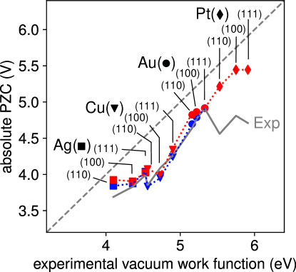
Figure 8: Relative trend of PZC values as obtained in experiments and implicit solvent calculations. Experimental PZCs for the low-index surfaces of Ag, Cu, Au and Pt (gray line) are on the absolute scale and taken as averages of literature data compiled in the SI of ref. 26. Calculated PZCs are arbitrarily aligned to the experimental PZC of Au(111) and taken from refs. 26 (red) and 313 (blue).

A corresponding comparison with experimental data in water is shown in Fig. 8 and reveals that even the fully implicit models employed in the corresponding studies capture this trend qualitatively, if not semi-quantitatively. As also apparent from Fig. 8, experimental absolute PZCs are consistently smaller than the corresponding vacuum work functions.^{338, 333, 339, 340, 324} In Fig. 8 the computed PZC values were arbitrarily aligned to the experimental PZC of Au(111) to illustrate the trend behavior, so that from there no conclusion can be drawn in how much implicit solvation models can reproduce this reduction. However, if the implicit water-vacuum drop is indeed small, then one can indeed show that they would effectively yield this reduction, albeit likely only on a quantitatively smaller scale.^{313, 341, 342, 26}. This is actually surprising, since the reduction originates in reality mainly from finite charge transfer from water molecules in the inner DL and a concomitant polarization within the first $\sim 4$ Å away from the metal surface.^{343, 344, 56} Outliers to the captured trend in the PZCs, e.g. the larger offset for Pt visible in Fig. 8, have been ascribed to an increased interfacial charge transfer that can no longer be mimicked by the implicit solvation model.⁵⁶ However, for more reactive surfaces one also has to keep in mind that experimental PZCs can not least be influenced by specifically adsorbed electrolyte ions^{331, 345}. If the calculations were repeated for a corresponding chemical composition $N_{\alpha}$ including such ions, the agreement might thus improve. However, in general, this uncertainty is nothing but a consequence of the ”poor man’s sampling” in ab initio thermodynamics, which requires the explicit testing of different such chemical compositions $N_{\alpha}$, rather than yielding the true equilibrium one as an outcome of the theory.

3.3 Computational hydrogen electrode

Many of the thermodynamic quantities that are of central interest in electrocatalysis concern energetics. Take the surface free energy as a measure of the stability of the catalyst surface, or adsorption free energies as central to the surface thermochemistry (or within Brønsted-Evans-Polanyi relationships^{346, 347, 348} even indicative of the reaction kinetics). Computing or evaluating such energetic quantities within the ab initio thermodynamics framework described in Section 3.1 almost invariably involves comparing the relative stability of interface configurations with different chemical composition $N_{\alpha}$. Next to the electron electrochemical potential referencing issues discussed in the preceding section, this then also puts the electrochemical potentials of particle species $\alpha$ like explicitly described ions, solvent molecules or electrode constituents on the agenda. In addition, the energetic quantities are typically not only required at the PZC, which could then bring up first trouble with the charge restriction of prevalent periodic boundary DFT supercell implementations.

Let us exemplify this general problem in this section for the simple case of hydrogen adsorption (formally better proton electrosorption) in an aqueous environment. A pertinent thermodynamic quantity to compute for this case is the adsorption free energy. Within the ab initio thermodynamics ansatz this is suitably defined as an applied-potential dependent difference of fixed-composition total grand potential energies before and after the adsorption,

$$\Delta G^{{\rm ads},N_{\alpha}}_{\rm H}(\Phi_{\rm E})=\tilde{\Omega}^{N_{\alpha},{\rm H}}[\rho^{\circ}_{\mathrm{el,H}}(\Phi_{\rm E})]-\tilde{\Omega}^{N_{\alpha}}[\rho^{\circ}_{\mathrm{el}}(\Phi_{\rm E})]\quad.$$ (38)

Here, $N_{\alpha}$ summarizes the entire chemical composition of the electrode, which we assume to be unchanged upon adsorption apart from the additional proton (H nucleus). For simplicity of notation, we consider here only one proton per supercell, even though one would in the implicit solvation context practically prefer symmetric slab setups with adsorption of one proton per surface and thus two protons per supercell. Obviously, within the employed periodic boundary conditions adsorption of this proton per supercell corresponds as always effectively to some finite coverage, but this does not matter for our present argument. Note also that similarly as in Section 2.6 we again attest to the fact that (measurable) adsorption free energies are generally seen as a property of the full (macroscopic) system and not of the grand-canonical sub-system technically employed in the calculations, which is why we denote them as free energies even though they are computed here as a difference of grand potential energies.

Each fixed-composition total grand potential energy in eq. (38) is evaluated at its optimized equilibrium electron density. Due to the presence of the additional H nucleus, $\rho^{\circ}_{\rm el,H}$ will not only differ in its detailed spatial form from $\rho^{\circ}_{\rm el}$, but will generally also integrate up to a total number of electrons that differs by $l_{\mathrm{}}$—the so-called electrosorption valency ^{349, 350, 351, 352, 353, 354, 355, 356, 357, 358, 359, 360, 361, 362, 363, 324, 364, 365, 366, 367}. With the electrode chemical composition unchanged, the dependence on all electrode chemical potentials $\mu_{\rm sub}$ cancels in the difference of eq. (38). What remains are the electrochemical potentials of the bulk reservoirs from where the proton and the additional electron density dragged to it upon adsorption came from. At the electrified interface in the aqueous environment this correspond to $\tilde{\mu}_{\rm H^{+}}$ of the solvated proton and the electron electrochemical potential $\tilde{\mu}_{\rm el}$ as determined by the applied potential. Using eq. (37) we can thus rewrite eq. (38) as a difference of grand potential energies and these electrochemical potentials

$$\Delta G^{{\rm ads},N_{\alpha}}_{\rm H}(\Phi_{\rm E})=\left(\Omega^{N_{\alpha},{\rm H}}[\rho^{\circ}_{\mathrm{el,H}}(\Phi_{\mathrm{E}})]-\Omega^{N_{\alpha}}[\rho^{\circ}_{\mathrm{el}}(\Phi_{\mathrm{E}})]\right)-\left(\tilde{\mu}_{\rm H^{+}}+l_{\mathrm{}}\tilde{\mu}_{\rm el}\right)\quad.$$ (39)

This equation now clearly carves out the entire wealth of practical problems that have to be dealt with. Under an applied potential $\Phi_{\rm E}$ away from the PZC, the electrode will generally be charged with a corresponding balancing counter charge built up in the electrolyte. Some of this counter charge will be located in the diffuse DL, which is likely outside of a practically feasible DFT supercell as discussed in Chapter 1. Unless this is suitably taken care of by an implicit electrolyte model as discussed in the next section, this would imply the computation of charged supercells. Furthermore, to evaluate eq. (39) we also need to determine the two electrochemical potentials. While we have already seen the difficulties to align $\tilde{\mu}_{\rm el}=-e\Phi_{\rm E}$ on the absolute scale with the DFT-internal Fermi level in an implicit solvation calculation in the last section, also the explicit computation of the electrochemical potential of a solvated proton $\tilde{\mu}_{\mathrm{H}^{+}}$ is a tough endeavor^{368, 369, 370}.

Intriguingly, all of these problems vanish completely with just one single and ingenious approximation. If we assume that the optimized electron density of a given interface configuration $N_{\alpha}$ at any applied potential $\Phi_{\rm E}$ remains the same as the one at its PZC, then there is no electrolyte counter charge as discussed in the previous section and the DFT supercell is always charge neutral. For $\rho^{\circ}_{\mathrm{el,H}}$ this implies that the adsorbed protonic charge is exactly compensated by one additional electron, i.e. the H adsorption (proton electrosorption) process is a so-called proton-coupled electron transfer (PCET).^{371, 372} In turn, $l_{\mathrm{}}=1$ and we arrive at

$$\Delta G^{{\rm ads},N_{\alpha}}_{\rm H,CHE}(\Phi_{\rm E})=\left(\Omega^{N_{\alpha},{\rm H}}[\rho^{\circ}_{\mathrm{el,H}}(\Phi_{\mathrm{E,H,PZC}})]-\Omega^{N_{\alpha}}[\rho^{\circ}_{\mathrm{el}}(\Phi_{\mathrm{E,PZC}})]\right)-\left(\tilde{\mu}_{\rm H^{+}}+\tilde{\mu}_{\rm el}\right)\quad.$$ (40)

Also, the electrochemical potential calculation and alignment problem is naturally resolved, as the remaining integer sum of the two potentials in eq. (40) is simply related to the applied potential $\Phi_{\rm E}^{\rm SHE}$ on the SHE scale,^{332, 324, 373}

$$\left(\tilde{\mu}_{\rm H^{+}}+\tilde{\mu}_{\rm el}\right)\;=\;\tfrac{1}{2}\mu_{\mathrm{H_{2}}}-e\Phi^{\rm SHE}_{\rm E}-k_{\rm B}T\ln(10)\rm{pH}\quad.$$ (41)

Here, $\mu_{\mathrm{H_{2}}}$ is the chemical potential of hydrogen gas at standard state, which is straightforward to compute,^{373, 374, 375, 376, 13} and pH is the pH value of the aqueous electrolyte. Note that the SHE scale is the predominantly employed scale in experiments anyway, which thus does allow to directly compare with experiments (as long as they are not affected by mass transport effects^{41, 377}). There is correspondingly no need anymore to align the DFT-internal Fermi level to the applied potential. In fact, as the difference of grand potential energies in eq. (40) is now potential-independent, it suffices to compute it once, and the entire dependence of the adsorption free energy on the applied potential is then just analytically given by eq. (41). This analytic dependence becomes even easier on the reversible hydrogen electrode (RHE) scale,

$$\left(\tilde{\mu}_{\rm H^{+}}+\tilde{\mu}_{\rm el}\right)\;=\;\tfrac{1}{2}\mu_{\mathrm{H_{2}}}-e\Phi^{\rm RHE}_{\rm E}\quad,$$ (42)

i.e. all pH dependencies are in the CHE just trivially Nernstian.

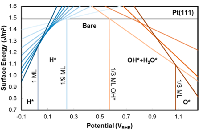
Figure 9: Surface phase diagram of Pt(111) in water as determined within the CHE approach. Shown are computed potential-dependent surface free energies of bare Pt(111) and various H, OH and O coverages on it. Within the ab initio thermodynamics framework, surface terminations with lowest surface free energy are declared as most stable one at the corresponding potential. This yields the indicated gradual transition from H-covered over bare surface to OH- and O-covered terminations with increasingly positive potential. Reproduced with permission from ref. 378.

The original intention to exploit the SHE definition to circumvent the electrochemical potential referencing issues was coined computational hydrogen electrode (CHE) by Rossmeisl, Nørskov and coworkers.^{373, 374} Nowadays, CHE is instead essentially equated with the somewhat stronger approximation to employ PZC optimized densities as introduced in the example above. This kind of CHE approach underlies the by far dominant part of contemporary first-principles based work on electrified interfaces and electrocatalysis at them. In fact, it is fair to say that without the computational simplicity enabled by the CHE, theoretical electrocatalysis would not be where it is today.³⁷⁹ The CHE philosophy is readily generalized to other electrodes (computational sulfur electrode, computational Li electrode,$\ldots$)^{380, 381, 382} and employed for the computation of other thermodynamic quantities. Notably, these are the aforementioned surface free energies^{14, 383, 384, 385, 386, 378, 387, 377}, i.e. the cost to create a surface with a certain structure and composition, as well as thermodynamic reaction barriers or concomitant thermodynamic overpotentials^{373, 374, 388, 389, 390, 391}. Using the prior applied-potential dependent surface free energies to compare the stability of a range of candidate surface structures and composition, one can readily establish surface phase diagrams, which—if the electrochemical potential dependence is resolved into a potential and pH dependence—are also known as Pourbaix diagrams. Figure 9 illustrates this with corresponding work from McCrum et al. for the Pt(111) surface in a water environment. Such kind of CHE surface phase diagrams are nowadays widely used to draw first conclusions on the actual surface structure and composition of electrodes under true operating conditions and we refer to excellent reviews on this topic^{1, 388, 392, 393, 379, 394} for a more detailed overview of the uses and merits of this kind of most popular CHE application.

If employed within the sketched CHE approach, the task of an implicit solvation model is to account for the solvation response at the PZC of the considered surface configuration. This is conceptually analogous to what was discussed in the previous section for the pristine electrode, yet with two notable, opposing differences. On the one hand, in particular for larger, more protruding, polar or hydrogen-bond affine adsorbates one can in principle expect larger solvation corrections even at the PZC.^{395, 396, 395, 397, 398, 43, 47} On the other hand, as apparent from eq. (40) it is typically differences of grand potential energies that matter for the targeted thermodynamic energetic quantities and in these differences solvation corrections partly cancel. As an upshot, such corrections to adsorption free energies by fully implicit solvation models are typically small for the prototypical adsorbates of interest in aqueous environments in particular for *H and *O, while being slightly larger for *OH, *OOH or *H₂O, maybe reaching up to some hundred meVs for the dipolar species. By and large, this seems to agree with the results of calculations with explicit solvent,^{399, 389, 397, 400} but this is most likely just due to fortuitous error cancellation in such free energy differences rather than evidence for the accuracy of present-day implicit solvation models and their existing parametrizations. More detailed analysis of the contributions points out that an arguably most important correction to existing schemes would be to account for so-called competitive solvent adsorption in the cavitation grand potential. This reflects the fact that in a thermodynamically consistent treatment of solvation at SLIs, there should be an energy cost associated with the need to first remove solvent from the pristine electrode to create space for the adsorbate. This would generally be a substrate-dependent cost,^{401, 65} in contrast to the existing, substrate agnostic cavitation grand potential formulations discussed in Section 2.4.1.

We think it could mainly be this missing appropriate account of competitive solvent adsorption that stands behind the (partly) dramatic discrepancies between implicit solvation results and benchmark AIMD simulations in explicit water environments.^{402, 43, 44} This view would be supported by the strong correlations with the OH/H₂O adsorption properties of the substrate⁴⁴. Note, however, that competitive solvent adsorption is also not appropriately considered in a wide range of simple explicit solvation strategies,^{373, 400} while it is generally questionable anyway whether the limited trajectories obtained in the dynamic simulations can really faithfully mimic thermodynamic equilibrium. On the implicit solvation side, there are some hints that more substrate-specific models such as the SCSS model using soft-sphere atomic cavities might constitute a way forward while not compromising other observables.³³⁷ Nevertheless, while all of this surely indicates the need to further advance implicit solvation models (or to rather move over to mixed explicit/implicit solvation models for SLIs), the fact remains that in a CHE free energy difference like in eq. (40) for the adsorption free energy, solvation corrections evaluated at the PZCs tend to be small. One can correspondingly find multiple practitioner works in the literature, where the CHE is applied and in fact no solvation treatment is included at all, i.e. the underlying DFT calculations are actually performed for slabs in vacuum. In historical perspective, the advent of implicit solvation methodology in major periodic boundary conditions DFT packages came after the CHE approximation was firmly established and widely employed by the theoretical electrocatalysis community. The new functionality was then often employed within the prevalent CHE, rather than realizing that it could actually constitute a powerful avenue beyond it.

3.4 Surface charging and interfacial capacitance

It is indeed important to realize that the typically small solvation corrections within the CHE are an invariable outcome of the PZC assumption. To assess this assumption, let us recall the physical processes actually occurring at a pristine electrode on gradual application of a potential that brings us away from its PZC. Without loss of generality, let this be a potential positive from the PZC, which will thus withdraw electrons from the electrode and lead to the formation of a positive net surface charge on the electrode surface. In order to screen the resulting electric field, a compensating counter charge will build up in the electrolyte part of the DL. Initially, this is just a capacitive charging process of the electric DL as introduced in Chapter 1. This means that the concomitant changes to the electrode electron density might induce some atomic relaxation or even stronger rearrangements in the electrode material. Also, the molecular and ionic distributions within the electrolyte will obviously change when building up the counter charge. However, at the initially small potentials there is formally no exchange of (charged) matter between these two constituents of the DL. In a fully implicit solvation model, this would thus mean that the chemical composition $N_{\alpha}$ of the DFT-part of the system does not change.

Upon further increase of the potential away from the PZC, the polarization of the DL might eventually become so large, that such an exchange will occur, specifically in form of a so-called interfacial (or Faradaic) charge transfer. Here, it is now generally the transfer of ions to or from the electrolyte with a concomitant change of their charge state that reduces the electric field. For the considered positive potential and an aqueous electrolyte, this could for instance be the specific adsorption of anions,^{403, 404, 405, 406, 407, 408, 409} or depending on the pH, the formation of hydroxyl groups at the metal electrode.^{410, 411, 412} Even in a fully implicit solvation model, these new surface species would be explicitly modeled and we would correspondingly arrive at a new chemical composition $N_{\alpha^{\prime}}$. This new electrode configuration then has its own new PZC,⁴¹³ typically at a more positive potential as the original pristine surface (cf. normal vs anomalous work function change⁴¹⁴). When now further increasing the potential, we are again moving away from this PZC and the sequence of capacitive charging and interfacial charge transfer upon exceeding DL polarization continues.

What the CHE does is to approximate this sequence with a series of pure charge-transfer processes through unpolarized electrode configurations. As it only considers the electron density at the PZC of each electrode configuration, it is agnostic to capacitive charging. The increasing applied potential enters the fixed-composition total grand potential only through the changed electron electrochemical potential term as in the hydrogen adsorption eq. (40) above. Within the ab initio thermodynamics framework, any change of relative stability of different electrode configurations can thus only be captured, if the concomitant change of $N_{\alpha}$ includes a change in the involved number of electrons $N_{\rm el}$, as is the case for an interfacial charge transfer. By construction, the CHE approximation can therefore for instance not account for potential-induced geometric changes or stronger reconstructions of the electrode that leave the chemical composition $N_{\alpha}$ unchanged.

In order to overcome these limitations of the CHE it is therefore imperative to include some form of surface charging into the modeling. Remember that one of the motivations for historically introducing the CHE was the charge-neutrality restriction of prevalent periodic boundary condition DFT implementations. This restriction is elegantly addressed by the PZC assumption as the electron density then automatically integrates up to exactly match the total nuclei charge of the DFT part of the supercell. Yet, even in these codes there is in practice nothing that prevents us from adding more or less electrons into the DFT calculation to mimic surface charging. What the codes would only do (more or less unnoticed), is to introduce a homogeneous background charge that exactly compensates the net charge that would result from this varied electron number.^{320, 246} In principle, this straightforward, so-called jellium approach can still be and is in fact largely used to model a potential-dependent electron density.^{415, 416, 417} Obviously though, a homogeneous background charge—if applied without further corrections—is unlikely a good representation of the DL counter charge and there are several studies that highlight the nonphysical surface charging behavior obtained within this approach.^{342, 320, 202}

It is especially to this problem of surface charging where implicit solvation methodology adds significant flexibility. As discussed in Section 2.5 and summarized in Fig. 5, current electrolyte models offer a wide spectrum of introducing counter ions into the supercell, thereby allowing to establish overall charge neutrality without the need for a jellium background. This spectrum ranges from the simple PCC Helmholtz-layer models to the self-consistent ion distributions of PB or MPB theory, where, importantly, the ion distributions described in the latter theories include the diffuse DL. Here, it is worthwhile to emphasize the elegance with which these implicit approaches solve the problem of the wide extension of the diffuse DL part highlighted in Chapter 1. Even if this extension largely exceeds the actual dimension of the supercell employed in the practical DFT calculation, this still plays no role as it only enters the generalized Poisson equation solver of the code, cf. Section 2.5. Corresponding solvers can be implemented with free boundary conditions in $z$-direction,^{243, 242} i.e. vertical to the slab surface, and are then completely independent of the finite supercell size used in the other parts of the KS DFT minimization. Whatever the specific electrolyte model used, its ionic counter charges thus flexibly allow to satisfy the supercell charge-neutrality condition despite a varying net surface charge on the explicitly DFT-described electrode. The implementation of corresponding implicit electrolyte models in a range of major DFT packages as summarized in Table 2 marked therefore a big conceptual step forward for the first-principles based modeling of electrified SLIs. What remains to be seen though, is what this actually brings practically for the modeling of surface charging and the truly intended computation of fixed-composition total grand potential energies $\tilde{\Omega}^{N_{\alpha}}[\rho_{\rm el}^{\circ}(\Phi_{\rm E})]$ with potential-dependent optimized electron densities $\rho_{\rm el}^{\circ}(\Phi_{\rm E})$, cf. eq. (37). Which aspects of the implicit physical counter charge model are truly important and how influential is the parametrization of the effective solvation model?

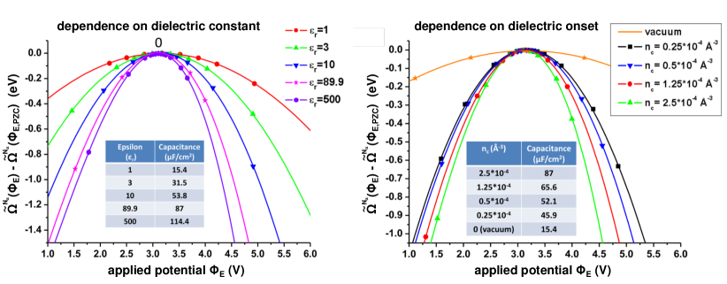
Figure 10: Dependence of the interfacial capacitance on implicit solvation model parameters. Shown is the variation of the fixed-composition total grand potential energy $\tilde{\Omega}^{N_{\alpha}}$ around the PZC for a model Li(110) electrode in implicit ethylene carbonate (EC) solvent ($\varepsilon(\mathrm{exp})=89.9$) . The parabolic variation nicely reflects the Taylor expansion of eq. (43) and allows to fit the interfacial capacitance. (Left panel) Variation as a function of the bulk permittivity employed in the implicit solvation model. (Right panel) Variation as a function of the threshold charge density (called $n_{\rm c}$) employed to define the solvation cavity. Adapted from ref. 382.

For a first such assessment it is instructive to perform a Taylor expansion of $\tilde{\Omega}^{N_{\alpha}}[\rho_{\rm el}^{\circ}(\Phi_{\rm E})]$ around the PZC, which can be achieved fully analytically up to second order ³⁶⁵

$$\tilde{\Omega}^{N_{\alpha}}[\rho_{\rm el}^{\circ}(\Phi_{\rm E})]=\tilde{\Omega}^{N_{\alpha}}[\rho_{\rm el}^{\circ}(\Phi_{\rm E,PZC})]-\frac{AC_{\mathrm{PZC}}}{2}\left(\Phi_{\rm E}-\Phi_{\rm E,PZC}\right)^{2}+\mathcal{O}(\left(\Phi_{\rm E}-\Phi_{\rm E,PZC}\right)^{3})\quad,$$ (43)

with $C_{\mathrm{PZC}}$ the area normalized interfacial capacitance at the PZC, and $A$ the surface area (which in practice in a symmetric slab calculation would comprise the upper and lower side of the slab). Consistent with the above discussed physics of capacitive charging when moving away from the PZC, it is thus $C_{\mathrm{PZC}}$ that naturally appears in the thermodynamics as a central quantity. This analysis correspondingly suggests that next to the PZC discussed in Section 3.2, implicit electrolyte models should especially be able to appropriately describe the capacitance $C_{\rm PZC}$ at the PZC to achieve a sound potential-dependence of grand potential energies $\tilde{\Omega}^{N_{\alpha}}[\rho_{\rm el}^{\circ}(\Phi_{\rm E})]$ away from the PZC. Figure 10 from Lespes and Filhol ³⁸² illustrates that in principle already fully-implicit models can offer this capability. Their data for Li(110) nicely portrays the inverted parabolas of the Taylor expansion, eq. (43), and the sensitive dependence of the extracted capacitance $C_{\rm PZC}$ on central parameters of the implicit solvation model, namely the bulk permittivity value and the iso-surface value of the electron density defining the solvation cavity, cf. Section 2.3. Note in particular the small capacitance values obtained in vacuum that can only be increased when considering the polarization response of the surrounding liquid through the implicit solvation model.

Further away from the PZC, higher-order terms in the Taylor expansion of eq. (43) will start to play a role, which will then feature variations of the interfacial capacitance with the applied potential. As a result, quite some work has been dedicated to construct implicit models that can reproduce experimentally observed capacitance variations with applied potential as well as electrolyte composition.^{172, 21, 309} As already introduced in Chapter 1, the total interfacial capacitance can be seen as arising from two capacitors in series, the inner DL and the outer DL. For high electrolyte concentrations or for potentials far away from the PZC, this total capacitance will correspondingly be dominated by the capacitance of the inner DL, where the highest potential drop occurs.³³ Consistent with this picture, the modeling of the diffuse DL is often found to play a minor role to describe the interfacial capacitance in this limit.^{40, 41} Instead, it is the appropriate parametrization of the solvation cavity boundary that critically determines the overall accuracy,⁴¹⁸ and it is within this understanding that refined models that include nonlinear electrolyte and dielectric response e.g. in form of a dielectric decrement as discussed in Section 2.5.3 are currently being pursued.³⁰⁹

3.5 Constant potential vs. constant charge calculations

As discussed in Section 3.3, the capability to compute applied-potential dependent fixed-composition total grand potential energies $\tilde{\Omega}^{N_{\alpha}}[\rho_{\rm el}^{\circ}(\Phi_{\rm E})]$ is a key prerequisite to access thermodynamic energetic quantities like surface free energies or adsorption free energies, see e.g. eq. (38) for the discussed example of hydrogen adsorption. To this end, the flexibility with which implicit electrolyte models allow to consider finite surface charges in the periodic DFT supercell calculations provides primarily an opportunity to go beyond the CHE approximation. Within the prevalent canonical DFT implementations that work with a prescribed number of electrons $N_{\rm el}$, the amount of surface charge that corresponds to a particular applied potential $\Phi_{\rm E}$ can e.g. straightforwardly be obtained from the condition that the DFT-internal electron chemical potential has to equal the external electron electrochemical potential at equilibrium. As discussed before in Section 3.2, the prior is given by the Fermi level position $\phi_{\rm F}(N_{\rm el})$ with respect to the DFT-internal vacuum reference $\phi_{\rm vac}$, while the latter is imposed by the applied potential. Thus, $N_{\rm el}(\Phi_{\rm E})$ is determined by varying the number of electrons in the calculation until

$$e(\phi_{\rm F}(N_{\rm el})-\phi_{\rm vac})=\tilde{\mu}_{\rm el}=-e\Phi_{\rm E}$$ (44)

is fulfilled.^{419, 342, 326, 420} For this electron number, the desired fixed-composition total grand potential energy is then evaluated as

$$\tilde{\Omega}^{N_{\alpha}}[\rho_{\rm el}^{\circ}(\Phi_{\rm E})]=\Omega^{N_{\alpha}}[\rho^{\circ}_{\mathrm{el}}(N_{\mathrm{el}}(\Phi_{\mathrm{E}}))]+e\Phi_{\mathrm{E}}N_{\mathrm{el}}(\Phi_{\mathrm{E}})\quad,$$ (45)

which mathematically can be identified as a Legendre transformation between the variables $N_{\rm el}$ and $\Phi_{\rm E}$. Equivalent results can be achieved via the use of a potentiostat⁴²¹ or in grand canonical DFT via an extended Hamiltonian.²³ Note that, if it is of interest to understand the interface energetics for a range of applied potentials, it can be computationally more efficient to simply compute $\Omega^{N_{\alpha}}[\rho^{\circ}_{\mathrm{el}}(N_{\mathrm{el}})]$ as well as $\Phi_{\mathrm{E}}(N_{\mathrm{el}})$ ($\leftrightarrow\phi_{\rm F}(N_{\rm el})$) for a set of electron numbers $\left\{N_{\mathrm{el}}\right\}$ from which the (continuous) $\tilde{\Omega}^{N_{\alpha}}[\rho_{\rm el}^{\circ}(\Phi_{\rm E})]$ can then be obtained in a straightforward way e.g. via interpolation²⁶.

In principle, correspondingly determined $\tilde{\Omega}^{N_{\alpha}}[\rho_{\rm el}^{\circ}(\Phi_{\rm E})]$ still suffer from the difficulty of referencing to the DFT-internal vacuum reference $\phi_{\rm vac}$ in implicit solvation calculations as discussed in Section 3.2. However, fortunately only differences of such fixed-composition total grand potential energies are typically required for targeted quantities like an adsorption free energy. In such differences, one can consistently reference to the available bulk implicit solvent potential, which then only implies a residual constant shift of the potential dependence of a quantity like $\Delta G^{{\rm ads},N_{\alpha}}(\Phi_{\rm E})$ with respect to an experimental scale. Accepting such constant uncertainty, empirical values are then also conveniently taken for additionally required electrochemical potentials of those particle species that vary in these differences, like the $\tilde{\mu}_{{\rm H}^{+}}$ of a solvated proton in the hydrogen adsorption example.

On the other hand, the necessity to evaluate differences also creates challenges, in particular with respect to the implicit solvation modeling. To understand this, let us recap the equation with which the hydrogen adsorption free energy of Section 3.3 would be determined in this constant-potential approach

$$\Delta G^{{\rm ads},N_{\alpha}}_{\rm H}(\Phi_{\rm E})=\tilde{\Omega}^{N_{\alpha},{\rm H}}[\rho^{\circ}_{\mathrm{el,H}}(\Phi_{\rm E})]-\tilde{\Omega}^{N_{\alpha}}[\rho^{\circ}_{\mathrm{el}}(\Phi_{\rm E})]\quad.$$ (46)

Both fixed-composition total grand potential energies are obviously here evaluated at the same applied potential $\Phi_{\rm E}$. However, as discussed in the last section, the PZCs of the H-covered and the clean surface are generally different. This means that the evaluation of the two grand potential energies proceeds at a different relative potential with respect to the respective PZC. It could for example be that the applied potential is actually quite close to the PZC of the clean surface, but rather far away from the H-covered one. In the last section we had seen that the accuracy of implicit electrolyte models typically depends on this relative difference from the PZC. A model might be better suited to describe the potential region around the PZC, while another one is tailored just for the inner DL-dominated region far away from the PZC. In the difference of eq. (46), the model can instead be required to describe quite different relative potential regions and this could introduce quite some error.

Aiming for better error cancelation, we can revisit the CHE and emphasize an aspect of it that is actually often overlooked. As discussed, the prevalent form of the CHE assumes that the optimized electron density of a given interface configuration $N_{\alpha}$ at any applied potential $\Phi_{\rm E}$ always remains the same as at its PZC, cf. Section 3.3. Intriguingly, this implies that in the difference required for the adsorption free energy, the two fixed-composition grand potential energies are actually evaluated at different potentials. In the hydrogen adsorption case and the corresponding eq. (40), this would namely be at the PZC of the hydrogen-covered surface $\Phi_{\rm E,H,PZC}$ and at the PZC of the clean surface $\Phi_{\rm E,PZC}$. It is now tempting to transfer this aspect to the surface charging case. If both terms in eq. (46) were not evaluated at the same potential, but at the same amount of surface charging, then both fixed-composition total grand potential energies are determined at an approximately equal relative potential with respect to their PZC and one can hope for maximum error cancellation in the implicit model. Of course, on the other hand, error is introduced because at least one of the two terms is not computed at the correct applied potential—but possibly this incurred error is smaller than the error cancellation achieved.

This is essentially the philosophy of so-called constant-charge calculations, which can in principle be carried out with explicit^{422, 423, 38} or implicit^{40, 41, 424, 425, 426, 427} charging. In such calculations the amount of surface charge according to an applied electrode potential is determined e.g. from experimental ³³ or simulated^{40, 41} charge-potential relations. The resulting decoupling of quantum chemistry and surface charging thus allows to control the accuracy of both scales roughly independently. While clearly inspired by the CHE, it is worthwhile to note that this approach is also closely related to traditional constant field calculations^{428, 39, 429, 430, 431, 37, 432, 373, 433, 434, 435, 436} as interfacial fields are naturally proportional to surface charge, and it is correspondingly not surprising that latter calculations were also taken into consideration in the early developments of the CHE approximation.^{428, 434, 373, 374, 429, 433}

Both the constant-potential^{419, 342, 326, 26, 420, 421, 23, 244, 245, 24, 437, 325} and constant-charge^{436, 430, 244, 40, 431, 424, 41, 425, 426, 427} approach enjoy present popularity, with the former also often denoted as fully grand-canonical (FGC) approach. While they give quantitatively different results in practical supercell sizes, it is gratifying that in the thermodynamic limit of low-coverage adsorption, i.e. one adsorbate in a laterally infinitely extended supercell, both approaches will eventually coincide.²⁴⁵ In this limit, the PZC of the clean surface will only be infinitesimally changed upon adsorption. At any applied potential, both the single-adsorbate covered and clean surface will thus be equally charged anyway, and one is in both cases also at an equal absolute and relative potential with respect to the joint PZC. For this limit, one can analogously to the constant-potential case also consider a constant-charge appropriate Taylor series expansion of the adsorption free energy, i.e. now in terms of the excess charge.^{245, 40, 365} Here it has been found that in many cases, the first order term corresponding to the PZC change is dominating. In contrast, higher-order terms depending on the capacitance and thus electrolyte description are indeed less relevant, supporting the error cancelation motivation of this approach.⁴⁰ For the constant-potential case, a dipole-field-type first-order correction term to the CHE adsorption free energy can even analytically be derived.^{244, 365, 367, 40, 41} For the specific example of hydrogen adsorption, this term reads

$$\Delta G^{{\rm ads},N_{\alpha}}_{\rm H(\theta\rightarrow 0)}(\Phi_{\rm E})-\Delta G^{{\rm ads},N_{\alpha}}_{\rm H(\theta\rightarrow 0),CHE}(\Phi_{\rm E})\approx e\;(l-1)\;(\Phi_{\rm E}-\Phi_{\rm E,PZC})\quad,$$ (47)

with the already earlier introduced electrosorption valency $l$ as measure of the number of electrons dragged onto the electrode upon adsorption of the proton. In the CHE, $l_{\rm CHE}=1$, corresponding to a PCET process, while in general $l\neq 1$.

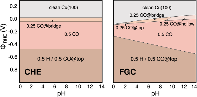
Figure 11: Theoretical surface Pourbaix diagram of Cu(100) in implicit water considering H and CO adsorbates. The diagram obtained within the CHE approximation (left panel) shows only a trivial Nernstian pH-dependence, which vanishes on the here employed RHE scale. In contrast, non-trivial pH-dependencies are obtained with constant-potential aka FGC calculations (right panel). Figure created from data published in ref. 438.

Compared to the CHE, changes in the potential-dependence of adsorption free energies as obtained in emerging constant-potential or constant-charge calculations seem indeed generally largely be understandable in terms of dipole-field interaction, even for larger molecules, such as e.g. CO₂ reduction intermediates⁴³⁹. Changes in this dipole-field interaction with applied potential can then lead to a wide range of conceptual physics that was outside of the realm of CHE theory. This includes a potential-induced switching of the most stable adsorption site^{26, 110, 435} or altered adsorbate geometries or adsorption motives^{440, 419}, including e.g. interfacial water⁴⁴¹. Recent corresponding results have for instance also helped to clarify the impact of different cationic species^{442, 40} on the interfacial capacitance^{443, 40, 39}, and how this can influence in an indirect way via the variation in the dipole-field interaction a variety of electrochemical observables such as the stability of adsorbed CO₂^{439, 40, 424, 110} and the Stark shifts of CO^{444, 445, 40}. In addition, the now available possibility to appropriately account for effects of the applied potential beyond the CHE has enabled significant progress in the simulation of electrochemical reaction barriers^{342, 244} and bridged the gap to works that employ explicit charging strategies.^{446, 447, 448, 449, 450, 244, 326, 422, 423} Further works reported potential-induced surface reconstructions or lifting of those^{451, 26} as well as non-Nernstian dependencies for surface coverages^{452, 26, 23, 453, 454, 178}, nanoparticle shapes^{452, 26}, Pourbaix diagrams^{438, 455, 456}, and last but not least (thermodynamic) cyclic voltammograms ^{26, 366, 367, 437}, where peak positions and shapes can indeed be extremely sensitive to the electrochemical conditions^{412, 457}. These developments are all quite recent and we expect significant further progress in our understanding of interfacial electrocatalysis to emerge from such constant-potential or constant-charge calculations³⁹⁴. As one final example we only highlight in Fig. 11 how constant-potential calculations help to overcome the trivially Nernstian pH-dependence of the CHE approach, cf. eq.(42). In the Pourbaix diagram for Cu(100) shown on the RHE potential scale, there is correspondingly no further pH dependence within the CHE, but significant structure when computed with the constant potential approach.

4 Conclusions and outlook

Predictive-quality first-principles calculations based on DFT have undoubtedly become a cornerstone in modern materials, catalysis and energy research. In the specific context of catalysis at electrified interfaces, this development is largely connected with the ingenious computational hydrogen electrode (CHE) approach of Rossmeisl, Nørskov and coworkers.^{373, 374} It is difficult to understate the impact that this single approach has made on the design of electrocatalysts or the unraveling of electrochemical reaction mechanisms.^{1, 388, 392, 393, 379, 394} By the very nature of its approximation, the CHE puts the predominant emphasis on the electrode site. Over the last decade or so, first-principles electrocatalysis research at solid-liquid interfaces (SLIs) was correspondingly dominated by finding optimum catalyst materials that lie at the top of reaction volcanos or gaining mechanistic understanding in terms of surface chemical bonds, yet without much caring for the electrolyte side of the SLI.

It is only within the last few years that an ever increasing understanding of electrified SLIs starts to trigger a return to this foundational pillar of electrochemistry, namely the influence of the electrolyte at the SLI.^{116, 114, 32, 458, 113, 115} Unfortunately, it is also only when one starts to devise strategies of how to actually do so within the realm of present-day DFT and supercomputer capabilities, that one really starts to appreciate the ingenuity of the CHE approximation and the simplicity of the calculations it enables. Any real consideration of the extended double layer (DL) with its intricate long-range electrostatics and inherent dynamics quickly leads to excessive computational costs. In this respect, implicit solvation methodology forms a unique compromise. As we have surveyed in this review, consideration of corresponding methodology within the ab initio thermodynamics framework commonly employed in surface catalysis anyway, immediately gives rise to multiple avenues beyond the CHE. At the same time, the computational cost of corresponding constant potential or constant charge calculations stays not too different from the one of the CHE approach.

While thus highly promising, this approach is not without its own challenges. The implementation of implicit solvation functionality into a series of powerful DFT software packages that can describe extended SLIs typically within the frame of periodic boundary condition supercells has been the enabler for this new field and a great community effort. However, in these implementations the methodological framework, historically developed to assess solvation effects on molecular solutes, has largely been left unaltered. To one end, this concerns the usage of parametrizations derived from molecular experimental reference data. To the other end, functional expressions for the effectively treated explicit electrode - implicit electrolyte interactions have if at all only marginally been modified, for instance if they contained quantities like a cavity volume that is not accessible at an extended SLI. As we have seen in the course of this review, the primary advance brought about by implicit solvation for the SLI context is more the flexibility with which one can represent the counter charges in the DL, rather than the actual account of solvation effects. For this purpose, the present state-of-the-art may largely be sufficient—and in addition to the already obtained massive insight into catalysis at electrified interfaces, we expect truly grand-canonical results (like the discussed constant potential or constant charge calculations) on the basis of existing implicit electrolyte models to continue carving out important electrochemistry that was not accessible within the CHE framework.

However, this can only be a first step. At present, the community is at a crossroad. One route is to focus efforts towards mixed explicit/implicit solvation approaches. The other is to refine the implicit solvation technology itself. For both case, what will centrally be required is a re-thinking of the functional expressions, in particular of the non-electrostatic terms, and reference data that is more pertinent for extended SLIs. Regarding the latter, we have seen throughout the review, that many experimentally accessible quantities commonly measured in electrochemistry are not ideal for this task, as their computation intricately mixes solvation effects with the specificities of the employed ab initio thermodynamics ansatz. In this respect, more, systematic and accurate measurements of PZCs and interfacial capacitances for well-defined model electrodes would certainly be helpful. In our view, also contact angles could be another highly useful class of quantities. Without any such data, it is largely impossible to develop highly parametrized and thus potentially more accurate implicit solvation methods without running into overfitting. From this perspective, the actual developments of first-principles machine-learned interatomic potentials are probably most exciting.^{81, 82} Explicit AIMD data^{368, 369, 459, 56, 460, 69, 461, 66, 68, 43, 44, 58, 462, 335, 463, 464} has long been used to validate and improve implicit solvation methodology. If machine-learned interatomic potentials allow to generate comparably accurate, but orders of magnitude longer trajectories and in larger simulation cells, then this will be an invaluable asset that might even ultimately enable to validate and refine implicit solvation schemes for application outside the domain of ab initio thermodynamics, notably the modeling of kinetic reaction barriers.

5 Acknowledgements

S.R. acknowledges funding from the National Research Foundation (NRF-2019R1A2C2086770), (NRF-2021R1C1C1008776) funded by the Korea Ministry of Science, ICT & Future Planning. N.G.H., H.O., and K.R. gratefully acknowledge funding by the Deutsche Forschungsgemeinschaft (DFG, German Research Foundation) under Germany’s Excellence Strategy – EXC 2089/1 – 390776260, as well as under project RE1509/35-1. N.G.H. acknowledges financial support through the EuroTech Postdoc Programme which is co-funded by the European Commission under its framework programme Horizon 2020 and Grant Agreement number 754462. H.O. further acknowledges funding by the Deutsche Forschungsgemeinschaft (DFG, German Research Foundation) through its Heisenberg program, grant No. OB 425-9/1. The authors acknowledge the core developers of the DFT program packages that helped in confirming the correctness of the content in Table 2, as well as thank the developers of the implicit solvation functionality in these codes for their great service to the community.

References

- Seh et al. 2017 Seh, Z. W.; Kibsgaard, J.; Dickens, C. F.; Chorkendorff, I.; Nørskov, J. K.; Jaramillo, T. F. Combining theory and experiment in electrocatalysis: Insights into materials design. Science 2017, 355
- Gür 2018 Gür, T. M. Review of electrical energy storage technologies, materials and systems: challenges and prospects for large-scale grid storage. Energy Environ. Sci. 2018, 11, 2696–2767
- Nong et al. 2020 Nong, H. N.; Falling, L. J.; Bergmann, A.; Klingenhof, M.; Tran, H. P.; Spöri, C.; Mom, R.; Timoshenko, J.; Zichittella, G.; Knop-Gericke, A. et al. Key role of chemistry versus bias in electrocatalytic oxygen evolution. Nature 2020, 587, 408–413
- Chen et al. 2019 Chen, Z. W.; Chen, L. X.; Wen, Z.; Jiang, Q. Understanding electro-catalysis by using density functional theory. Phys. Chem. Chem. Phys. 2019, 21, 23782–23802
- He et al. 2019 He, Q.; Yu, B.; Li, Z.; Zhao, Y. Density functional theory for battery materials. Energy Environ. Mater. 2019, 2, 264–279
- Urban et al. 2016 Urban, A.; Seo, D.-H.; Ceder, G. Computational understanding of Li-ion batteries. Npj Comput. Mater. 2016, 2, 1–13
- Nørskov et al. 2011 Nørskov, J. K.; Abild-Pedersen, F.; Studt, F.; Bligaard, T. Density functional theory in surface chemistry and catalysis. Proc. Natl. Acad. Sci. U. S. A. 2011, 108, 937–943
- Hammes-Schiffer and Galli 2021 Hammes-Schiffer, S.; Galli, G. Integration of theory and experiment in the modelling of heterogeneous electrocatalysis. Nat. Energy 2021, 6, 700–7005
- Khatib et al. 2021 Khatib, R.; Kumar, A.; Sanvito, S.; Sulpizi, M.; Cucinotta, C. S. The nanoscale structure of the Pt-water double layer under bias revealed. Electrochimica Acta 2021, 391, 138875
- Bruix et al. 2019 Bruix, A.; Margraf, J. T.; Andersen, M.; Reuter, K. First-principles-based multiscale modelling of heterogeneous catalysis. Nature Catalysis 2019, 2, 659–670
- Greeley 2016 Greeley, J. Theoretical Heterogeneous Catalysis: Scaling Relationships and Computational Catalyst Design. Annu. Rev. Chem. Biomol. Eng. 2016, 7, 605–635
- Reuter et al. 2017 Reuter, K.; Plaisance, C. P.; Oberhofer, H.; Andersen, M. Perspective: On the active site model in computational catalyst screening. J. Chem. Phys. 2017, 146, 040901
- Reuter 2016 Reuter, K. Ab Initio Thermodynamics and First-Principles Microkinetics for Surface Catalysis. Catal. Lett. 2016, 146, 541–563
- Reuter and Scheffler 2001 Reuter, K.; Scheffler, M. Composition, structure, and stability of RuO 2 (110) as a function of oxygen pressure. Phys. Rev. B 2001, 65, 035406
- Reuter and Scheffler 2004 Reuter, K.; Scheffler, M. Oxide formation at the surface of late 4d transition metals: insights from first-principles atomistic thermodynamics. Appl. Phys. A: Mater. Sci. Process. 2004, 78, 793–798
- Rogal et al. 2004 Rogal, J.; Reuter, K.; Scheffler, M. Thermodynamic stability of PdO surfaces. Phys. Rev. B 2004, 69, 075421
- Stampfl 2005 Stampfl, C. Surface processes and phase transitions from ab initio atomistic thermodynamics and statistical mechanics. Catal. Today 2005, 105, 17–35
- Reuter et al. 2005 Reuter, K.; Stampf, C.; Scheffler, M. In Handbook of Materials Modeling: Methods; Yip, S., Ed.; Springer Netherlands: Dordrecht, 2005; pp 149–194
- Rogal and Reuter 2006 Rogal, J.; Reuter, K. Ab initio atomistic thermodynamics for surfaces: A primer; 2006
- Trindell et al. 2019 Trindell, J. A.; Duan, Z.; Henkelman, G.; Crooks, R. M. Well-defined nanoparticle electrocatalysts for the refinement of theory. Chem. Rev. 2019, 120, 814–850
- Schwarz and Sundararaman 2020 Schwarz, K.; Sundararaman, R. The electrochemical interface in first-principles calculations. Surf. Sci. Rep. 2020, 75, 100492
- Sundararaman and Schwarz 2017 Sundararaman, R.; Schwarz, K. Evaluating continuum solvation models for the electrode-electrolyte interface: Challenges and strategies for improvement. J. Chem. Phys. 2017, 146, 084111
- Sundararaman et al. 2017 Sundararaman, R.; Goddard, W. A., 3rd; Arias, T. A. Grand canonical electronic density-functional theory: Algorithms and applications to electrochemistry. J. Chem. Phys. 2017, 146, 114104
- Gauthier et al. 2019 Gauthier, J. A.; Ringe, S.; Dickens, C. F.; Garza, A. J.; Bell, A. T.; Head-Gordon, M.; Nørskov, J. K.; Chan, K. Challenges in Modeling Electrochemical Reaction Energetics with Polarizable Continuum Models. ACS Catal. 2019, 9, 920–931
- Nattino et al. 2019 Nattino, F.; Truscott, M.; Marzari, N.; Andreussi, O. Continuum models of the electrochemical diffuse layer in electronic-structure calculations. J. Chem. Phys. 2019, 150, 041722
- Hörmann et al. 2019 Hörmann, N. G.; Andreussi, O.; Marzari, N. Grand canonical simulations of electrochemical interfaces in implicit solvation models. J. Chem. Phys. 2019, 150, 041730
- Tomasi 2004 Tomasi, J. Thirty years of continuum solvation chemistry: a review, and prospects for the near future. Theor. Chem. Acc. 2004, 112, 184–203
- Tomasi et al. 2005 Tomasi, J.; Mennucci, B.; Cammi, R. Quantum mechanical continuum solvation models. Chem. Rev. 2005, 105, 2999–3093
- Cramer and Truhlar 1999 Cramer, C. J.; Truhlar, D. G. Implicit Solvation Models: Equilibria, Structure, Spectra, and Dynamics. Chem. Rev. 1999, 99, 2161–2200
- Eftekhari-Bafrooei and Borguet 2011 Eftekhari-Bafrooei, A.; Borguet, E. Effect of electric fields on the ultrafast vibrational relaxation of water at a charged solid–liquid interface as probed by vibrational sum frequency generation. J. Phys. Chem. Lett. 2011, 2, 1353–1358
- Nihonyanagi et al. 2013 Nihonyanagi, S.; Mondal, J. A.; Yamaguchi, S.; Tahara, T. Structure and dynamics of interfacial water studied by heterodyne-detected vibrational sum-frequency generation. Annu. Rev. Phys. Chem. 2013, 64, 579–603
- Helmholtz 1853 Helmholtz, H. Ueber einige Gesetze der Vertheilung elektrischer Ströme in körperlichen Leitern, mit Anwendung auf die thierisch-elektrischen Versuche (Schluss.). Ann. Phys. 1853, 165, 353–377
- Parsons 1997 Parsons, R. The metal-liquid electrolyte interface. Solid State Ionics 1997, 94, 91–98
- Lockett et al. 2010 Lockett, V.; Horne, M.; Sedev, R.; Rodopoulos, T.; Ralston, J. Differential capacitance of the double layer at the electrode/ionic liquids interface. Phys. Chem. Chem. Phys. 2010, 12, 12499–12512
- Fumagalli et al. 2018 Fumagalli, L.; Esfandiar, A.; Fabregas, R.; Hu, S.; Ares, P.; Janardanan, A.; Yang, Q.; Radha, B.; Taniguchi, T.; Watanabe, K. et al. Anomalously low dielectric constant of confined water. Science 2018, 360, 1339–1342
- Kornyshev et al. 2007 Kornyshev, A. A.; Spohr, E.; Vorotyntse, M. A. In Encyclopedia of Electrochemistry; Bard, A. J., Ed.; Techn. Report no 14 to the office of Naval Research of Febr. 18, 1954; Wiley-VCH Verlag GmbH & Co. KGaA: Weinheim, Germany, 2007; Vol. 41; p 2307
- Chen et al. 2016 Chen, L. D.; Urushihara, M.; Chan, K.; Nørskov, J. K. Electric Field Effects in Electrochemical CO2 Reduction. ACS Catal. 2016, 6, 7133–7139
- Sandberg et al. 2016 Sandberg, R. B.; Montoya, J. H.; Chan, K.; Nørskov, J. K. CO-CO coupling on Cu facets: Coverage, strain and field effects. Surf. Sci. 2016, 654, 56–62
- Resasco et al. 2017 Resasco, J.; Chen, L. D.; Clark, E.; Tsai, C.; Hahn, C.; Jaramillo, T. F.; Chan, K.; Bell, A. T. Promoter Effects of Alkali Metal Cations on the Electrochemical Reduction of Carbon Dioxide. J. Am. Chem. Soc. 2017, 139, 11277–11287
- Ringe et al. 2019 Ringe, S.; Clark, E. L.; Resasco, J.; Walton, A.; Seger, B.; Bell, A. T.; Chan, K. Understanding cation effects in electrochemical CO2 reduction. Energy Environ. Sci. 2019, 12, 3001–3014
- Ringe et al. 2020 Ringe, S.; Morales-Guio, C. G.; Chen, L. D.; Fields, M.; Jaramillo, T. F.; Hahn, C.; Chan, K. Double layer charging driven carbon dioxide adsorption limits the rate of electrochemical carbon dioxide reduction on Gold. Nat. Commun. 2020, 11, 33
- Delle Site et al. 2007 Delle Site, L.; Ghiringhelli, L. M.; Andreussi, O.; Donadio, D.; Parrinello, M. The interplay between surface–water and hydrogen bonding in a water adlayer on Pt (111) and Ag (111). J. Phys. Condens. Matter 2007, 19, 242101
- Ludwig et al. 2019 Ludwig, T.; Gauthier, J. A.; Brown, K. S.; Ringe, S.; Nørskov, J. K.; Chan, K. Solvent–Adsorbate Interactions and Adsorbate-Specific Solvent Structure in Carbon Dioxide Reduction on a Stepped Cu Surface. J. Phys. Chem. C 2019, 123, 5999–6009
- Heenen et al. 2020 Heenen, H. H.; Gauthier, J. A.; Kristoffersen, H. H.; Ludwig, T.; Chan, K. Solvation at metal/water interfaces: An ab initio molecular dynamics benchmark of common computational approaches. J. Chem. Phys. 2020, 152, 144703
- Ludwig et al. 2020 Ludwig, T.; Gauthier, J. A.; Dickens, C. F.; Brown, K. S.; Ringe, S.; Chan, K.; Nørskov, J. K. Atomistic Insight into Cation Effects on Binding Energies in Cu-Catalyzed Carbon Dioxide Reduction. J. Phys. Chem. C 2020, 124, 24765–24775
- Oberhofer 2020 Oberhofer, H. In Handbook of Materials Modeling: Applications: Current and Emerging Materials; Andreoni, W., Yip, S., Eds.; Springer International Publishing: Cham, 2020; pp 1505–1537
- Gauthier et al. 2017 Gauthier, J. A.; Dickens, C. F.; Chen, L. D.; Doyle, A. D.; Nørskov, J. K. Solvation Effects for Oxygen Evolution Reaction Catalysis on IrO2(110). J. Phys. Chem. C 2017, 121, 11455–11463
- Tomasi and Persico 1994 Tomasi, J.; Persico, M. Molecular interactions in solution: An overview of methods based on continuous distributions of the solvent. Chem. Rev. 1994, 94, 2027–2094
- Kirkwood 1934 Kirkwood, J. G. Theory of solutions of molecules containing widely separated charges with special application to zwitterions. J. Chem. Phys. 1934, 2, 351–361
- Onsager 1936 Onsager, L. Electric moments of molecules in liquids. J. Am. Chem. Soc. 1936, 58, 1486–1493
- Hassanali et al. 2014 Hassanali, A. A.; Cuny, J.; Verdolino, V.; Parrinello, M. Aqueous solutions: state of the art in ab initio molecular dynamics. Philos. Trans. A Math. Phys. Eng. Sci. 2014, 372, 20120482
- Iftimie et al. 2005 Iftimie, R.; Minary, P.; Tuckerman, M. E. Ab initio molecular dynamics: concepts, recent developments, and future trends. Proc. Natl. Acad. Sci. U. S. A. 2005, 102, 6654–6659
- VandeVondele et al. 2005 VandeVondele, J.; Mohamed, F.; Krack, M.; Hutter, J.; Sprik, M.; Parrinello, M. The influence of temperature and density functional models in ab initio molecular dynamics simulation of liquid water. J. Chem. Phys. 2005, 122, 14515
- Gillan et al. 2016 Gillan, M. J.; Alfè, D.; Michaelides, A. Perspective: How good is DFT for water? J. Chem. Phys. 2016, 144, 130901
- Groß et al. 2014 Groß, A.; Gossenberger, F.; Lin, X.; Naderian, M.; Sakong, S.; Roman, T. Water structures at metal electrodes studied by ab initio molecular dynamics simulations. J. Electrochem. Soc. 2014, 161, E3015–E3020
- Le et al. 2017 Le, J.; Iannuzzi, M.; Cuesta, A.; Cheng, J. Determining Potentials of Zero Charge of Metal Electrodes versus the Standard Hydrogen Electrode from Density-Functional-Theory-Based Molecular Dynamics. Phys. Rev. Lett. 2017, 119, 016801
- Gaiduk et al. 2015 Gaiduk, A. P.; Gygi, F.; Galli, G. Density and Compressibility of Liquid Water and Ice from First-Principles Simulations with Hybrid Functionals. J. Phys. Chem. Lett. 2015, 6, 2902–2908
- Ambrosio et al. 2016 Ambrosio, F.; Miceli, G.; Pasquarello, A. Structural, Dynamical, and Electronic Properties of Liquid Water: A Hybrid Functional Study. J. Phys. Chem. B 2016, 120, 7456–7470
- Chen et al. 2017 Chen, M.; Ko, H.-Y.; Remsing, R. C.; Calegari Andrade, M. F.; Santra, B.; Sun, Z.; Selloni, A.; Car, R.; Klein, M. L.; Perdew, J. P. et al. Ab initio theory and modeling of water. Proc. Natl. Acad. Sci. U. S. A. 2017, 114, 10846–10851
- Zheng et al. 2018 Zheng, L.; Chen, M.; Sun, Z.; Ko, H.-Y.; Santra, B.; Dhuvad, P.; Wu, X. Structural, electronic, and dynamical properties of liquid water by ab initio molecular dynamics based on SCAN functional within the canonical ensemble. J. Chem. Phys. 2018, 148, 164505
- Ruiz Pestana et al. 2018 Ruiz Pestana, L.; Marsalek, O.; Markland, T. E.; Head-Gordon, T. The Quest for Accurate Liquid Water Properties from First Principles. J. Phys. Chem. Lett. 2018, 9, 5009–5016
- Hammer et al. 1999 Hammer, B.; Hansen, L. B.; Nørskov, J. K. Improved adsorption energetics within density-functional theory using revised Perdew-Burke-Ernzerhof functionals. Phys. Rev. B 1999, 59, 7413–7421
- Grimme et al. 2010 Grimme, S.; Antony, J.; Ehrlich, S.; Krieg, H. A consistent and accurate ab initio parametrization of density functional dispersion correction (DFT-D) for the 94 elements H-Pu. J. Chem. Phys. 2010, 132, 154104
- Grimme et al. 2016 Grimme, S.; Hansen, A.; Brandenburg, J. G.; Bannwarth, C. Dispersion-Corrected Mean-Field Electronic Structure Methods. Chem. Rev. 2016, 116, 5105–5154
- Tonigold and Gross 2012 Tonigold, K.; Gross, A. Dispersive interactions in water bilayers at metallic surfaces: a comparison of the PBE and RPBE functional including semiempirical dispersion corrections. J. Comput. Chem. 2012, 33, 695–701
- Sakong et al. 2016 Sakong, S.; Forster-Tonigold, K.; Groß, A. The structure of water at a Pt(111) electrode and the potential of zero charge studied from first principles. J. Chem. Phys. 2016, 144, 194701
- Ando et al. 2013 Ando, Y.; Gohda, Y.; Tsuneyuki, S. Ab initio molecular dynamics study of the Helmholtz layer formed on solid–liquid interfaces and its capacitance. Chem. Phys. Lett. 2013, 556, 9–12
- Sakong and Groß 2018 Sakong, S.; Groß, A. The electric double layer at metal-water interfaces revisited based on a charge polarization scheme. J. Chem. Phys. 2018, 149, 084705
- Le et al. 2020 Le, J.-B.; Fan, Q.-Y.; Li, J.-Q.; Cheng, J. Molecular origin of negative component of Helmholtz capacitance at electrified Pt(111)/water interface. Sci Adv 2020, 6
- He et al. 2018 He, X.; Zhu, Y.; Epstein, A.; Mo, Y. Statistical variances of diffusional properties from ab initio molecular dynamics simulations. Npj Comput. Mater. 2018, 4, 1–9
- Harrison et al. 2018 Harrison, J. A.; Schall, J. D.; Maskey, S.; Mikulski, P. T.; Knippenberg, M. T.; Morrow, B. H. Review of force fields and intermolecular potentials used in atomistic computational materials research. Appl. Phys. Rev. 2018, 5, 031104
- Cisneros et al. 2016 Cisneros, G. A.; Wikfeldt, K. T.; Ojamäe, L.; Lu, J.; Xu, Y.; Torabifard, H.; Bartók, A. P.; Csányi, G.; Molinero, V.; Paesani, F. Modeling Molecular Interactions in Water: From Pairwise to Many-Body Potential Energy Functions. Chem. Rev. 2016, 116, 7501–7528
- Steinmann et al. 2018 Steinmann, S. N.; Ferreira De Morais, R.; Götz, A. W.; Fleurat-Lessard, P.; Iannuzzi, M.; Sautet, P.; Michel, C. Force Field for Water over Pt(111): Development, Assessment, and Comparison. J. Chem. Theory Comput. 2018, 14, 3238–3251
- Clabaut et al. 2020 Clabaut, P.; Fleurat-Lessard, P.; Michel, C.; Steinmann, S. N. Ten Facets, One Force Field: The GAL19 Force Field for Water-Noble Metal Interfaces. J. Chem. Theory Comput. 2020, 16, 4565–4578
- Buckley et al. 2019 Buckley, A. K.; Lee, M.; Cheng, T.; Kazantsev, R. V.; Larson, D. M.; Goddard, W. A., III; Toste, F. D.; Toma, F. M. Electrocatalysis at Organic-Metal Interfaces: Identification of Structure-Reactivity Relationships for CO2 Reduction at Modified Cu Surfaces. J. Am. Chem. Soc. 2019, 141, 7355–7364
- Senftle et al. 2016 Senftle, T. P.; Hong, S.; Islam, M. M.; Kylasa, S. B.; Zheng, Y.; Shin, Y. K.; Junkermeier, C.; Engel-Herbert, R.; Janik, M. J.; Aktulga, H. M. et al. The ReaxFF reactive force-field: development, applications and future directions. Npj Comput. Mater, 2016, 2, 1–14
- Liang et al. 2018 Liang, T.; Antony, A. C.; Akhade, S. A.; Janik, M. J.; Sinnott, S. B. Applied Potentials in Variable-Charge Reactive Force Fields for Electrochemical Systems. J. Phys. Chem. A 2018, 122, 631–638
- Onofrio and Strachan 2015 Onofrio, N.; Strachan, A. Voltage equilibration for reactive atomistic simulations of electrochemical processes. J. Chem. Phys. 2015, 143, 054109
- Onofrio et al. 2015 Onofrio, N.; Guzman, D.; Strachan, A. Atomic origin of ultrafast resistance switching in nanoscale electrometallization cells. Nat. Mater. 2015, 14, 440–446
- Xu et al. 2018 Xu, K.; Islam, M. M.; Guzman, D.; Seabaugh, A. C.; Strachan, A.; Fullerton-Shirey, S. K. Pulse Dynamics of Electric Double Layer Formation on All-Solid-State Graphene Field-Effect Transistors. ACS Appl. Mater. Interfaces 2018, 10, 43166–43176
- Ko et al. 2021 Ko, T. W.; Finkler, J. A.; Goedecker, S.; Behler, J. A fourth-generation high-dimensional neural network potential with accurate electrostatics including non-local charge transfer. Nature Commun. 2021, 12, 1–11
- Csanyi et al. 2021 Csanyi, G.; Deringer, V.; Bernstein, N.; Bartok, A.; Wilkins, D.; Ceriotti, M. Gaussian Process Regression for Materials and Molecules. Chem. Rev. 2021, accepted
- Kondati Natarajan and Behler 2017 Kondati Natarajan, S.; Behler, J. Self-Diffusion of Surface Defects at Copper–Water Interfaces. J. Phys. Chem. C 2017, 121, 4368–4383
- Natarajan and Behler 2016 Natarajan, S. K.; Behler, J. Neural network molecular dynamics simulations of solid-liquid interfaces: water at low-index copper surfaces. Phys. Chem. Chem. Phys. 2016, 18, 28704–28725
- Quaranta et al. 2017 Quaranta, V.; Hellström, M.; Behler, J. Proton-Transfer Mechanisms at the Water-ZnO Interface: The Role of Presolvation. J. Phys. Chem. Lett. 2017, 8, 1476–1483
- Lim et al. 2016 Lim, H.-K.; Lee, H.; Kim, H. A Seamless Grid-Based Interface for Mean-Field QM/MM Coupled with Efficient Solvation Free Energy Calculations. J. Chem. Theory Comput. 2016, 12, 5088–5099
- Stecher et al. 2016 Stecher, T.; Reuter, K.; Oberhofer, H. First-principles free-energy barriers for photoelectrochemical surface reactions: Proton abstraction at TiO 2 (110). Phys. Rev. Lett. 2016, 117, 276001
- Gim et al. 2018 Gim, S.; Lim, H.-K.; Kim, H. Multiscale Simulation Method for Quantitative Prediction of Surface Wettability at the Atomistic Level. J. Phys. Chem. Lett. 2018, 9, 1750–1758
- Gim et al. 2019 Gim, S.; Cho, K. J.; Lim, H.-K.; Kim, H. Structure, Dynamics, and Wettability of Water at Metal Interfaces. Sci. Rep. 2019, 9, 14805
- Naserifar et al. 2021 Naserifar, S.; Chen, Y.; Kwon, S.; Xiao, H.; Goddard, W. A. Artificial Intelligence and QM/MM with a Polarizable Reactive Force Field for Next-Generation Electrocatalysts. Matter 2021, 4, 195–216
- Bulo et al. 2009 Bulo, R. E.; Ensing, B.; Sikkema, J.; Visscher, L. Toward a practical method for adaptive QM/MM simulations. J. Chem. Theory Comput. 2009, 5, 2212–2221
- Watanabe et al. 2014 Watanabe, H. C.; Kubar, T.; Elstner, M. Size-consistent multipartitioning QM/MM: A stable and efficient adaptive QM/MM method. J. Chem. Theory Comput. 2014, 10, 4242–4252
- Watanabe and Cui 2019 Watanabe, H. C.; Cui, Q. Quantitative analysis of QM/MM boundary artifacts and correction in adaptive QM/MM simulations. J. Chem. Theory Comput. 2019, 15, 3917–3928
- Naserifar and Goddard 2018 Naserifar, S.; Goddard, W. A., 3rd The quantum mechanics-based polarizable force field for water simulations. J. Chem. Phys. 2018, 149, 174502
- Wu et al. 2006 Wu, Y.; Tepper, H. L.; Voth, G. A. Flexible simple point-charge water model with improved liquid-state properties. J. Chem. Phys. 2006, 124, 024503
- Zielkiewicz 2005 Zielkiewicz, J. Structural properties of water: Comparison of the SPC, SPCE, TIP4P, and TIP5P models of water. J. Chem. Phys. 2005, 123, 104501
- Wang and Van Voorhis 2012 Wang, L.-P.; Van Voorhis, T. A polarizable QM/MM explicit solvent model for computational electrochemistry in water. Journal of chemical theory and computation 2012, 8, 610–617
- Clabaut et al. 2020 Clabaut, P.; Schweitzer, B.; Götz, A. W.; Michel, C.; Steinmann, S. N. Solvation Free Energies and Adsorption Energies at the Metal/Water Interface from Hybrid QM-MM Simulations. J. Chem. Theor. Comput. 2020, 16, 6539–6549
- Beglov and Roux 1997 Beglov, D.; Roux, B. An integral equation to describe the solvation of polar molecules in liquid water. J. Phys. Chem. B 1997, 101, 7821–7826
- Hirata 2003 Hirata, F. Molecular Theory of Solvation; Springer Science & Business Media, 2003; Vol. 24
- Percus and Yevick 1958 Percus, J. K.; Yevick, G. J. Analysis of classical statistical mechanics by means of collective coordinates. Phys. Rev. 1958, 110, 1–13
- van Leeuwen et al. 1959 van Leeuwen, J. M. J.; Groeneveld, J.; de Boer, J. New method for the calculation of the pair correlation function. I. Physica 1959, 25, 792–808
- Kovalenko and Hirata 1999 Kovalenko, A.; Hirata, F. Self-consistent description of a metal–water interface by the Kohn–Sham density functional theory and the three-dimensional reference interaction site model. J. Chem. Phys. 1999, 110, 10095–10112
- Gusarov et al. 2006 Gusarov, S.; Ziegler, T.; Kovalenko, A. Self-consistent combination of the three-dimensional RISM theory of molecular solvation with analytical gradients and the Amsterdam density functional package. J. Phys. Chem. A 2006, 110, 6083–6090
- Nishihara and Otani 2017 Nishihara, S.; Otani, M. Hybrid solvation models for bulk, interface, and membrane: Reference interaction site methods coupled with density functional theory. Phys. Rev. B 2017, 96, 115429
- Haruyama et al. 2018 Haruyama, J.; Ikeshoji, T.; Otani, M. Analysis of Lithium Insertion/Desorption Reaction at Interfaces between Graphite Electrodes and Electrolyte Solution Using Density Functional + Implicit Solvation Theory. J. Phys. Chem. C 2018, 122, 9804–9810
- Zhan et al. 2018 Zhan, C.; Pham, T. A.; Cerón, M. R.; Campbell, P. G.; Vedharathinam, V.; Otani, M.; Jiang, D.-E.; Biener, J.; Wood, B. C.; Biener, M. Origins and Implications of Interfacial Capacitance Enhancements in C60-Modified Graphene Supercapacitors. ACS Appl. Mater. Interfaces 2018, 10, 36860–36865
- Zhan et al. 2019 Zhan, C.; Cerón, M. R.; Hawks, S. A.; Otani, M.; Wood, B. C.; Pham, T. A.; Stadermann, M.; Campbell, P. G. Specific ion effects at graphitic interfaces. Nat. Commun. 2019, 10, 4858
- Sugahara et al. 2019 Sugahara, A.; Ando, Y.; Kajiyama, S.; Yazawa, K.; Gotoh, K.; Otani, M.; Okubo, M.; Yamada, A. Negative dielectric constant of water confined in nanosheets. Nat. Commun. 2019, 10, 850
- Weitzner et al. 2020 Weitzner, S. E.; Akhade, S. A.; Varley, J. B.; Wood, B. C.; Otani, M.; Baker, S. E.; Duoss, E. B. Toward Engineering of Solution Microenvironments for the CO2 Reduction Reaction: Unraveling pH and Voltage Effects from a Combined Density-Functional-Continuum Theory. J. Phys. Chem. Lett. 2020, 11, 4113–4118
- Sundararaman et al. 2015 Sundararaman, R.; Schwarz, K. A.; Letchworth-Weaver, K.; Arias, T. A. Spicing up continuum solvation models with SaLSA: the spherically averaged liquid susceptibility ansatz. J. Chem. Phys. 2015, 142, 054102
- Bonthuis et al. 2012 Bonthuis, D. J.; Gekle, S.; Netz, R. R. Profile of the static permittivity tensor of water at interfaces: consequences for capacitance, hydration interaction and ion adsorption. Langmuir 2012, 28, 7679–7694
- Gouy 1910 Gouy, G. Constitution of the electric charge at the surface of an electrolyte. J. de Physique 1910, 9, 457–468
- Chapman 1913 Chapman, D. L. Theory of electrocapillarity. Philos. Mag. 1913, 25, 475–481
- Gouy 1916 Gouy, G. Sur la fonction électrocapillaire. Ann. Phys. 1916, 9, 5–36
- Debye and Hückel 1923 Debye, P.; Hückel, E. Theory of electrolytes. II. Law of the limit of electrolytic conductivity. Phys. Z. 1923, 24, 305–325
- Borukhov et al. 1997 Borukhov, I.; Andelman, D.; Orland, H. Steric Effects in Electrolytes: A Modified Poisson-Boltzmann Equation. Phys. Rev. Lett. 1997, 79, 435–438
- Becke 2014 Becke, A. D. Perspective: Fifty years of density-functional theory in chemical physics. J. Chem. Phys. 2014, 140, 18A301
- Hille et al. 2019 Hille, C.; Ringe, S.; Deimel, M.; Kunkel, C.; Acree, W. E.; Reuter, K.; Oberhofer, H. Generalized molecular solvation in non-aqueous solutions by a single parameter implicit solvation scheme. J. Chem. Phys. 2019, 150, 041710
- Ringe et al. 2017 Ringe, S.; Oberhofer, H.; Reuter, K. Transferable ionic parameters for first-principles Poisson-Boltzmann solvation calculations: Neutral solutes in aqueous monovalent salt solutions. J. Chem. Phys. 2017, 146, 134103
- Wilson 1998 Wilson, R. Classical Electrodynamics, 3rd ed.; Wiley: Hoboken, NJ, USA, 1998
- Slavchov 2014 Slavchov, R. I. Quadrupole terms in the Maxwell equations: Debye-Hückel theory in quadrupolarizable solvent and self-salting-out of electrolytes. J. Chem. Phys. 2014, 140, 164510
- Baumeier et al. 2014 Baumeier, B.; Rohlfing, M.; Andrienko, D. Electronic excitations in push–pull oligomers and their complexes with fullerene from many-body Green’s functions theory with polarizable embedding. J. Chem. Theory Comput. 2014, 10, 3104–3110
- Duchemin et al. 2016 Duchemin, I.; Jacquemin, D.; Blase, X. Combining the GW formalism with the polarizable continuum model: A state-specific non-equilibrium approach. J. Chem. Phys. 2016, 144, 164106
- Gunceler et al. 2013 Gunceler, D.; Letchworth-Weaver, K.; Sundararaman, R.; Schwarz, K. A.; Arias, T. A. The importance of nonlinear fluid response in joint density-functional theory studies of battery systems. Modell. Simul. Mater. Sci. Eng. 2013, 21, 074005
- Sundararaman and Goddard 2015 Sundararaman, R.; Goddard, W. A., 3rd The charge-asymmetric nonlocally determined local-electric (CANDLE) solvation model. J. Chem. Phys. 2015, 142, 064107
- Andreussi et al. 2019 Andreussi, O.; Hörmann, N. G.; Nattino, F.; Fisicaro, G.; Goedecker, S.; Marzari, N. Solvent-Aware Interfaces in Continuum Solvation. J. Chem. Theory Comput. 2019, 15, 1996–2009
- Bonthuis and Netz 2013 Bonthuis, D. J.; Netz, R. R. Beyond the continuum: how molecular solvent structure affects electrostatics and hydrodynamics at solid-electrolyte interfaces. J. Phys. Chem. B 2013, 117, 11397–11413
- Andreussi et al. 2012 Andreussi, O.; Dabo, I.; Marzari, N. Revised self-consistent continuum solvation in electronic-structure calculations. J. Chem. Phys. 2012, 136, 064102
- Ringe et al. 2016 Ringe, S.; Oberhofer, H.; Hille, C.; Matera, S.; Reuter, K. Function-Space-Based Solution Scheme for the Size-Modified Poisson-Boltzmann Equation in Full-Potential DFT. J. Chem. Theory Comput. 2016, 12, 4052–4066
- Sinstein et al. 2017 Sinstein, M.; Scheurer, C.; Matera, S.; Blum, V.; Reuter, K.; Oberhofer, H. Efficient Implicit Solvation Method for Full Potential DFT. J. Chem. Theory Comput. 2017, 13, 5582–5603
- Ringe 2017 Ringe, S. First-Principles Modeling in Poisson-Boltzmann Electrolytes. Ph.D. thesis, Technische Universität München, 2017
- Marenich et al. 2007 Marenich, A. V.; Olson, R. M.; Kelly, C. P.; Cramer, C. J.; Truhlar, D. G. Self-Consistent Reaction Field Model for Aqueous and Nonaqueous Solutions Based on Accurate Polarized Partial Charges. J. Chem. Theory Comput. 2007, 3, 2011–2033
- Klamt and Schüürmann 1993 Klamt, A.; Schüürmann, G. COSMO: a new approach to dielectric screening in solvents with explicit expressions for the screening energy and its gradient. J. Chem. Soc. Perkin Trans. 2 1993, 799–805
- Fisicaro et al. 2017 Fisicaro, G.; Genovese, L.; Andreussi, O.; Mandal, S.; Nair, N. N.; Marzari, N.; Goedecker, S. Soft-Sphere Continuum Solvation in Electronic-Structure Calculations. J. Chem. Theory Comput. 2017, 13, 3829–3845
- Fattebert and Gygi 2003 Fattebert, J.-L.; Gygi, F. First-principles molecular dynamics simulations in a continuum solvent. Int. J. Quantum Chem. 2003, 93, 139–147
- Petrosyan et al. 2005 Petrosyan, S. A.; Rigos, A. A.; Arias, T. A. Joint density-functional theory: ab initio study of Cr2O3 surface chemistry in solution. J. Phys. Chem. B 2005, 109, 15436–15444
- Sundararaman et al. 2014 Sundararaman, R.; Gunceler, D.; Arias, T. A. Weighted-density functionals for cavity formation and dispersion energies in continuum solvation models. J. Chem. Phys. 2014, 141, 134105
- Dupont et al. 2013 Dupont, C.; Andreussi, O.; Marzari, N. Self-consistent continuum solvation (SCCS): the case of charged systems. J. Chem. Phys. 2013, 139, 214110
- Truscott and Andreussi 2019 Truscott, M.; Andreussi, O. Field-Aware Interfaces in Continuum Solvation. J. Phys. Chem. B 2019, 123, 3513–3524
- Postma et al. 1982 Postma, J. P. M.; Berendsen, H. J. C.; Haak, J. R. Thermodynamics of cavity formation in water. A molecular dynamics study. Faraday Symposia of the Chemical Society. 1982; pp 55–67
- Pohorille and Pratt 1990 Pohorille, A.; Pratt, L. R. Cavities in molecular liquids and the theory of hydrophobic solubilities. J. Am. Chem. Soc. 1990, 112, 5066–5074
- Floris et al. 1997 Floris, F. M.; Selmi, M.; Tani, A.; Tomasi, J. Free energy and entropy for inserting cavities in water: Comparison of Monte Carlo simulation and scaled particle theory results. J. Chem. Phys. 1997, 107, 6353–6365
- Höfinger and Zerbetto 2005 Höfinger, S.; Zerbetto, F. Simple models for hydrophobic hydration. Chem. Soc. Rev. 2005, 34, 1012–1020
- Hummer et al. 1996 Hummer, G.; Garde, S.; García, A. E.; Pohorille, A.; Pratt, L. R. An information theory model of hydrophobic interactions. Proc. Natl. Acad. Sci. U. S. A. 1996, 93, 8951–8955
- Pratt 2002 Pratt, L. R. Molecular theory of hydrophobic effects: “She is too mean to have her name repeated.”. Annu. Rev. Phys. Chem. 2002, 53, 409–436
- Reiss et al. 1959 Reiss, H.; Frisch, H. L.; Lebowitz, J. L. Statistical mechanics of rigid spheres. J. Chem. Phys. 1959, 31, 369–380
- Reiss et al. 1960 Reiss, H.; Frisch, H. L.; Helfand, E.; Lebowitz, J. L. Aspects of the statistical thermodynamics of real fluids. J. Chem. Phys. 1960, 32, 119–124
- Pierotti 1976 Pierotti, R. A. A scaled particle theory of aqueous and nonaqueous solutions. Chem. Rev. 1976, 76, 717–726
- Langlet et al. 1977 Langlet, J.; Claverie, P.; Pullman, B.; Piazzola, D.; others, Studies of solvent effects. Theor. Chim. Acta 1977, 46, 105–116
- Cole 1957 Cole, R. H. Induced polarization and dielectric constant of polar liquids. J. Chem. Phys. 1957, 27, 33–35
- Mayer 1963 Mayer, S. W. A molecular parameter relationship between surface tension and liquid compressibility. J. Phys. Chem. 1963, 67, 2160–2164
- Wilhelm and Battino 1971 Wilhelm, E.; Battino, R. Estimation of Lennard-Jones (6, 12) Pair Potential Parameters from Gas Solubility Data. J. Chem. Phys. 1971, 55, 4012–4017
- Ben-Amotz and Willis 1993 Ben-Amotz, D.; Willis, K. G. Molecular hard-sphere volume increments. J. Phys. Chem. 1993, 97, 7736–7742
- Tang and Bloomfield 2000 Tang, K. E.; Bloomfield, V. A. Excluded volume in solvation: sensitivity of scaled-particle theory to solvent size and density. Biophys. J. 2000, 79, 2222–2234
- Uhlig 1937 Uhlig, H. H. The solubilities of gases and surface tension. J. Phys. Chem. 1937, 41, 1215–1226
- Tuñón et al. 1993 Tuñón, I.; Silla, E.; Pascual-Ahuir, J. L. Continuum-uniform approach calculations of the solubility of hydrocarbons in water. Chem. Phys. Lett. 1993, 203, 289–294
- Tolman 1949 Tolman, R. C. The effect of droplet size on surface tension. J. Chem. Phys. 1949, 17, 333–337
- Huang et al. 2001 Huang, D. M.; Geissler, P. L.; Chandler, D. Scaling of hydrophobic solvation free energies. J. Phys. Chem. B 2001, 105, 6704–6709
- Scherlis et al. 2006 Scherlis, D. A.; Fattebert, J.-L.; Gygi, F.; Cococcioni, M.; Marzari, N. A unified electrostatic and cavitation model for first-principles molecular dynamics in solution. J. Chem. Phys. 2006, 124, 74103
- Cococcioni et al. 2005 Cococcioni, M.; Mauri, F.; Ceder, G.; Marzari, N. Electronic-enthalpy functional for finite systems under pressure. Phys. Rev. Lett. 2005, 94, 145501
- Margenau and Kestner 2013 Margenau, H.; Kestner, N. R. Theory of Intermolecular Forces: International Series of Monographs in Natural Philosophy; Elsevier, 2013; Vol. 18
- Amovilli and Mennucci 1997 Amovilli, C.; Mennucci, B. Self-consistent-field calculation of Pauli repulsion and dispersion contributions to the solvation free energy in the polarizable continuum model. J. Phys. Chem. B 1997, 101, 1051–1057
- Floris et al. 1991 Floris, F. M.; Tomasi, J.; Ahuir, J. L. P. Dispersion and repulsion contributions to the solvation energy: Refinements to a simple computational model in the continuum approximation. J. Comput. Chem. 1991, 12, 784–791
- Piana et al. 2015 Piana, S.; Donchev, A. G.; Robustelli, P.; Shaw, D. E. Water dispersion interactions strongly influence simulated structural properties of disordered protein states. J. Phys. Chem. B 2015, 119, 5113–5123
- Hwang et al. 2015 Hwang, J.; Dial, B. E.; Li, P.; Kozik, M. E.; Smith, M. D.; Shimizu, K. D. How important are dispersion interactions to the strength of aromatic stacking interactions in solution? Chem. Sci. 2015, 6, 4358–4364
- Amovilli 1994 Amovilli, C. Calculation of the dispersion energy contribution to the solvation free energy. Chem. Phys. Lett. 1994, 229, 244–249
- McWeeny 1992 McWeeny, R. Methods of molecular quantum mechanics, 2nd ed.; Academic Press: San Diego, CA, 1992
- Still et al. 1990 Still, W. C.; Tempczyk, A.; Hawley, R. C.; Hendrickson, T. Semianalytical treatment of solvation for molecular mechanics and dynamics. J. Am. Chem. Soc. 1990, 112, 6127–6129
- Chowdhry et al. 2008 Chowdhry, B. Z.; Dines, T. J.; Jabeen, S.; Withnall, R. Vibrational spectra of -amino acids in the zwitterionic state in aqueous solution and the solid state: DFT calculations and the influence of hydrogen bonding. J. Phys. Chem. A 2008, 112, 10333–10347
- Ben-Naim 2013 Ben-Naim, A. Y. Solvation Thermodynamics; Springer Science & Business Media, 2013
- Andreussi and Fisicaro 2019 Andreussi, O.; Fisicaro, G. Continuum embeddings in condensed-matter simulations. Int. J. Quantum Chem. 2019, 119, e25725
- Gray and Stiles 2018 Gray, C. G.; Stiles, P. J. Nonlinear electrostatics: the Poisson–Boltzmann equation. Eur. J. Phys. 2018, 39, 053002
- Tetrode 1912 Tetrode, H. Die chemische Konstante der Gase und das elementare Wirkungsquantum. Ann. Phys. 1912, 343, 434–442
- Sackur 1911 Sackur, O. Die Anwendung der kinetischen Theorie der Gase auf chemische Probleme. Ann. Phys. 1911, 341, 958–980
- Sackur 1913 Sackur, O. Die universelle Bedeutung des sog. elementaren Wirkungsquantums. Ann. Phys. 1913, 345, 67–86
- Chipman 2004 Chipman, D. M. Solution of the linearized Poisson–Boltzmann equation. J. Chem. Phys. 2004, 120, 5566–5575
- Mathew et al. 2019 Mathew, K.; Kolluru, V. S. C.; Mula, S.; Steinmann, S. N.; Hennig, R. G. Implicit self-consistent electrolyte model in plane-wave density-functional theory. J. Chem. Phys. 2019, 151, 234101
- Kilic et al. 2007 Kilic, M. S.; Bazant, M. Z.; Ajdari, A. Steric effects in the dynamics of electrolytes at large applied voltages. II. Modified Poisson-Nernst-Planck equations. Phys. Rev. E 2007, 75, 021503
- Bikerman 1942 Bikerman, J. J. Structure and capacity of the electrical double layer. Philos. Mag. 1942, 33, 384
- Wang et al. 2013 Wang, H.; Thiele, A.; Pilon, L. Simulations of Cyclic Voltammetry for Electric Double Layers in Asymmetric Electrolytes: A Generalized Modified Poisson–Nernst–Planck Model. J. Phys. Chem. C 2013, 117, 18286–18297
- Borukhov et al. 2000 Borukhov, I.; Andelman, D.; Orland, H. Adsorption of large ions from an electrolyte solution: a modified Poisson–Boltzmann equation. Electrochim. Acta 2000, 46, 221–229
- Kralj-Iglič and Iglič 1996 Kralj-Iglič, V.; Iglič, A. A Simple Statistical Mechanical Approach to the free Energy of the Electric Double Layer Including the Excluded Volume Effect. J. Phys. II 1996, 6, 477–491
- Han et al. 2014 Han, Y.; Huang, S.; Yan, T. A mean-field theory on the differential capacitance of asymmetric ionic liquid electrolytes. J. Phys. Condens. Matter 2014, 26, 284103
- McEldrew et al. 2018 McEldrew, M.; Goodwin, Z. A. H.; Kornyshev, A. A.; Bazant, M. Z. Theory of the Double Layer in Water-in-Salt Electrolytes. J. Phys. Chem. Lett. 2018, 9, 5840–5846
- Kornyshev 2007 Kornyshev, A. A. Double-layer in ionic liquids: paradigm change? J. Phys. Chem. B 2007, 111, 5545–5557
- Popović and Šiber 2013 Popović, M.; Šiber, A. Lattice-gas Poisson-Boltzmann approach for sterically asymmetric electrolytes. Phys. Rev. E 2013, 88, 022302
- Maggs and Podgornik 2016 Maggs, A. C.; Podgornik, R. General theory of asymmetric steric interactions in electrostatic double layers. Soft Matter 2016, 12, 1219–1229
- May 2019 May, S. Differential capacitance of the electric double layer: mean-field modeling approaches. Current Opinion in Electrochemistry 2019, 13, 125–131
- Antypov et al. 2005 Antypov, D.; Barbosa, M. C.; Holm, C. Incorporation of excluded-volume correlations into Poisson-Boltzmann theory. Phys. Rev. E 2005, 71, 061106
- Burak and Andelman 2000 Burak, Y.; Andelman, D. Hydration interactions: aqueous solvent effects in electric double layers. Phys. Rev. E 2000, 62, 5296–5312
- Bohinc et al. 2012 Bohinc, K.; Shrestha, A.; Brumen, M.; May, S. Poisson-Helmholtz-Boltzmann model of the electric double layer: analysis of monovalent ionic mixtures. Phys. Rev. E 2012, 85, 031130
- Bohinc et al. 2011 Bohinc, K.; Shrestha, A.; May, S. The Poisson-Helmholtz-Boltzmann model. Eur. Phys. J. E 2011, 34, 108
- Bohinc et al. 2017 Bohinc, K.; Bossa, G. V.; May, S. Incorporation of ion and solvent structure into mean-field modeling of the electric double layer. Adv. Colloid Interface Sci. 2017, 249, 220–233
- Ben-Yaakov et al. 2011 Ben-Yaakov, D.; Andelman, D.; Podgornik, R.; Harries, D. Ion-specific hydration effects: Extending the Poisson-Boltzmann theory. Curr. Opin. Colloid Interface Sci. 2011, 16, 542–550
- Chandra 2000 Chandra, A. Static dielectric constant of aqueous electrolyte solutions: Is there any dynamic contribution? J. Chem. Phys. 2000, 113, 903–905
- Glueckauf 1964 Glueckauf, E. Bulk dielectric constant of aqueous electrolyte solutions. Trans. Faraday Soc. 1964, 60, 1637
- Wei and Sridhar 1990 Wei, Y.-Z.; Sridhar, S. Dielectric spectroscopy up to 20 GHz of LiCl/H2O solutions. J. Chem. Phys. 1990, 92, 923–928
- Wei et al. 1992 Wei, Y.-Z.; Chiang, P.; Sridhar, S. Ion size effects on the dynamic and static dielectric properties of aqueous alkali solutions. J. Chem. Phys. 1992, 96, 4569–4573
- Buchner et al. 1999 Buchner, R.; Hefter, G. T.; May, P. M. Dielectric relaxation of aqueous NaCl solutions. J. Phys. Chem. A 1999, 103, 1–9
- Ben-Yaakov et al. 2011 Ben-Yaakov, D.; Andelman, D.; Podgornik, R. Dielectric decrement as a source of ion-specific effects. J. Chem. Phys. 2011, 134, 074705
- Melander et al. 2019 Melander, M. M.; Kuisma, M. J.; Christensen, T. E. K.; Honkala, K. Grand-canonical approach to density functional theory of electrocatalytic systems: Thermodynamics of solid-liquid interfaces at constant ion and electrode potentials. J. Chem. Phys. 2019, 150, 041706
- Skinner et al. 2010 Skinner, B.; Loth, M. S.; Shklovskii, B. I. Capacitance of the double layer formed at the metal/ionic-conductor interface: how large can it be? Phys. Rev. Lett. 2010, 104, 128302
- Mezger et al. 2008 Mezger, M.; Schröder, H.; Reichert, H.; Schramm, S.; Okasinski, J. S.; Schöder, S.; Honkimäki, V.; Deutsch, M.; Ocko, B. M.; Ralston, J. et al. Molecular layering of fluorinated ionic liquids at a charged sapphire (0001) surface. Science 2008, 322, 424–428
- Bazant et al. 2011 Bazant, M. Z.; Storey, B. D.; Kornyshev, A. A. Double layer in ionic liquids: overscreening versus crowding. Phys. Rev. Lett. 2011, 106, 046102
- Levin 2002 Levin, Y. Electrostatic correlations: from plasma to biology. Rep. Prog. Phys. 2002, 65, 1577–1632
- Sahin and Ralf 2014 Sahin, B.; Ralf, B. Nonlocal and nonlinear electrostatics of a dipolar Coulomb fluid. J. Phys. Condens. Matter 2014, 26, 285101
- Buyukdagli and Blossey 2016 Buyukdagli, S.; Blossey, R. Beyond Poisson-Boltzmann: fluctuations and fluid structure in a self-consistent theory. J. Phys. Condens. Matter 2016, 28, 343001
- Li et al. 2014 Li, L.; Fennell, C. J.; Dill, K. A. Small molecule solvation changes due to the presence of salt are governed by the cost of solvent cavity formation and dispersion. J. Chem. Phys. 2014, 141, 22D518
- Marenich et al. 2009 Marenich, A. V.; Cramer, C. J.; Truhlar, D. G. Universal solvation model based on solute electron density and on a continuum model of the solvent defined by the bulk dielectric constant and atomic surface tensions. J. Phys. Chem. B 2009, 113, 6378–6396
- Mobley and Guthrie 2014 Mobley, D. L.; Guthrie, J. P. FreeSolv: a database of experimental and calculated hydration free energies, with input files. J. Comput. Aided Mol. Des. 2014, 28, 711–720
- Wang et al. 2016 Wang, B.; Zhao, Z.; Wei, G.-W. Automatic parametrization of non-polar implicit solvent models for the blind prediction of solvation free energies. J. Chem. Phys. 2016, 145, 124110
- Rizzo et al. 2006 Rizzo, R. C.; Aynechi, T.; Case, D. A.; Kuntz, I. D. Estimation of Absolute Free Energies of Hydration Using Continuum Methods: Accuracy of Partial Charge Models and Optimization of Nonpolar Contributions. J. Chem. Theory Comput. 2006, 2, 128–139
- Kelly et al. 2006 Kelly, C. P.; Cramer, C. J.; Truhlar, D. G. Aqueous solvation free energies of ions and ion-water clusters based on an accurate value for the absolute aqueous solvation free energy of the proton. J. Phys. Chem. B 2006, 110, 16066–16081
- Marenich et al. 2012 Marenich, A. V.; Kelly, C. P.; Thompson, J. D.; Hawkins, G. D.; Chambers, C. C.; Giesen, D. J.; Winget, P.; Cramer, C. J.; Truhlar, D. G. Minnesota Solvation Database – version 2012; 2012
- 216 Solv@TUM - The Solvation Free Energy Database on mediaTUM - Media and Publication Server. \urlhttp://doi.org/10.14459/2018mp1452571, Accessed: 2021-7-21
- 217 Solv@TUM - The Solvation Free Energy Database on github. \urlhttps://github.com/hille721/solvatum, Accessed: 2021-7-21
- Moine et al. 2017 Moine, E.; Privat, R.; Sirjean, B.; Jaubert, J.-N. Estimation of Solvation Quantities from Experimental Thermodynamic Data: Development of the Comprehensive CompSol Databank for Pure and Mixed Solutes. J. Phys. Chem. Ref. Data 2017, 46, 033102
- Oğuz et al. 2021 Oğuz, I. C.; Vassetti, D.; Labat, F. Assessing the performances of different continuum solvation models for the calculation of hydration energies of molecules, polymers and surfaces: a comparison between the SMD, VASPsol and FDPB models. Theor. Chem. Acc. 2021, 140, 99
- Alibakhshi and Hartke 2021 Alibakhshi, A.; Hartke, B. Improved prediction of solvation free energies by machine-learning polarizable continuum solvation model. Nat. Commun. 2021, 12, 3584
- Thompson et al. 2004 Thompson, J. D.; Cramer, C. J.; Truhlar, D. G. New universal solvation model and comparison of the accuracy of the SM5. 42R, SM5. 43R, C-PCM, D-PCM, and IEF-PCM continuum solvation models for aqueous and organic solvation free energies and for vapor pressures. J. Phys. Chem. A 2004, 108, 6532–6542
- Xu 2004 Xu, K. Nonaqueous liquid electrolytes for lithium-based rechargeable batteries. Chem. Rev. 2004, 104, 4303–4417
- König et al. 2019 König, M.; Vaes, J.; Klemm, E.; Pant, D. Solvents and Supporting Electrolytes in the Electrocatalytic Reduction of CO2. iScience 2019, 19, 135–160
- Koper 2013 Koper, M. T. M. Theory of multiple proton–electron transfer reactions and its implications for electrocatalysis. Chem. Sci. 2013, 4, 2710–2723
- Cardona et al. 2012 Cardona, T.; Sedoud, A.; Cox, N.; Rutherford, A. W. Charge separation in photosystem II: a comparative and evolutionary overview. Biochim. Biophys. Acta 2012, 1817, 26–43
- Jones 2007 Jones, M. Reviews of reactive intermediate chemistry; Wiley-Interscience: Hoboken, NJ, 2007
- McGrath et al. 2013 McGrath, M. J.; Kuo, I. W.; Ngouana W, B. F.; Ghogomu, J. N.; Mundy, C. J.; Marenich, A. V.; Cramer, C. J.; Truhlar, D. G.; Siepmann, J. I. Calculation of the Gibbs free energy of solvation and dissociation of HCl in water via Monte Carlo simulations and continuum solvation models. Phys. Chem. Chem. Phys. 2013, 15, 13578–13585
- Jinnouchi and Anderson 2008 Jinnouchi, R.; Anderson, A. B. Aqueous and Surface Redox Potentials from Self-Consistently Determined Gibbs Energies. J. Phys. Chem. C 2008, 112, 8747–8750
- Lewis et al. 1961 Lewis, G. N.; Randall, M.; Pitzer, K. S.; Brewer, L.; McGraw-Hill, Thermodynamics, 2nd ed.; 1961; p 399
- Pliego and Riveros 2002 Pliego, J. R., Jr; Riveros, J. M. Gibbs energy of solvation of organic ions in aqueous and dimethyl sulfoxide solutions. Phys. Chem. Chem. Phys. 2002, 4, 1622–1627
- Gupta et al. 2012 Gupta, M.; da Silva, E. F.; Svendsen, H. F. Modeling temperature dependency of amine basicity using PCM and SM8T implicit solvation models. J. Phys. Chem. B 2012, 116, 1865–1875
- Gupta et al. 2013 Gupta, M.; da Silva, E. F.; Svendsen, H. F. Modeling temperature dependency of ionization constants of amino acids and carboxylic acids. J. Phys. Chem. B 2013, 117, 7695–7709
- Liu et al. 2015 Liu, M.; Besford, Q. A.; Mulvaney, T.; Gray-Weale, A. Order and correlation contributions to the entropy of hydrophobic solvation. J. Chem. Phys. 2015, 142, 114117
- Chamberlin et al. 2008 Chamberlin, A. C.; Cramer, C. J.; Truhlar, D. G. Extension of a temperature-dependent aqueous solvation model to compounds containing nitrogen, fluorine, chlorine, bromine, and sulfur. J. Phys. Chem. B 2008, 112, 3024–3039
- Sechenow 1892 Sechenow, I. M. Ann. Chim. Phys. 1892, 25, 226
- Long and McDevit 1952 Long, F. A.; McDevit, W. F. Activity Coefficients of Nonelectrolyte Solutes in Aqueous Salt Solutions. Chem. Rev. 1952, 51, 119–169
- Mennucci et al. 1997 Mennucci, B.; Cancès, E.; Tomasi, J. Evaluation of solvent effects in isotropic and anisotropic dielectrics and in ionic solutions with a unified integral equation method: Theoretical bases, computational implementation, and numerical applications. J. Phys. Chem. B 1997, 101, 10506–10517
- Stein et al. 2019 Stein, C. J.; Herbert, J. M.; Head-Gordon, M. The Poisson-Boltzmann model for implicit solvation of electrolyte solutions: Quantum chemical implementation and assessment via Sechenov coefficients. J. Chem. Phys. 2019, 151, 224111
- Labat et al. 2018 Labat, F.; Civalleri, B.; Dovesi, R. Implicit Solvation Using a Generalized Finite-Difference Approach in CRYSTAL: Implementation and Results for Molecules, Polymers, and Surfaces. J. Chem. Theory Comput. 2018, 14, 5969–5983
- Cossi 2004 Cossi, M. Continuum solvation model for infinite periodic systems. Chem. Phys. Lett. 2004, 384, 179–184
- Delley 2006 Delley, B. The conductor-like screening model for polymers and surfaces. Mol. Simul. 2006, 32, 117–123
- Dabo et al. 2008 Dabo, I.; Kozinsky, B.; Singh-Miller, N. E.; Marzari, N. Electrostatics in periodic boundary conditions and real-space corrections. Phys. Rev. B 2008, 77, 115139
- Andreussi and Marzari 2014 Andreussi, O.; Marzari, N. Electrostatics of solvated systems in periodic boundary conditions. Phys. Rev. B 2014, 90, 245101
- Gauthier et al. 2019 Gauthier, J. A.; Dickens, C. F.; Heenen, H. H.; Vijay, S.; Ringe, S.; Chan, K. Unified Approach to Implicit and Explicit Solvent Simulations of Electrochemical Reaction Energetics. J. Chem. Theory Comput. 2019, 15, 6895–6906
- Gauthier et al. 2019 Gauthier, J. A.; Dickens, C. F.; Ringe, S.; Chan, K. Practical Considerations for Continuum Models Applied to Surface Electrochemistry. ChemPhysChem 2019, 20, 3074–3080
- Womack et al. 2018 Womack, J. C.; Anton, L.; Dziedzic, J.; Hasnip, P. J.; Probert, M. I. J.; Skylaris, C.-K. DL_MG: A Parallel Multigrid Poisson and Poisson-Boltzmann Solver for Electronic Structure Calculations in Vacuum and Solution. J. Chem. Theory Comput. 2018, 14, 1412–1432
- Fisicaro et al. 2016 Fisicaro, G.; Genovese, L.; Andreussi, O.; Marzari, N.; Goedecker, S. A generalized Poisson and Poisson-Boltzmann solver for electrostatic environments. J. Chem. Phys. 2016, 144, 014103
- Coons et al. 2016 Coons, M. P.; You, Z.-Q.; Herbert, J. M. The Hydrated Electron at the Surface of Neat Liquid Water Appears To Be Indistinguishable from the Bulk Species. J. Am. Chem. Soc. 2016, 138, 10879–10886
- Coons and Herbert 2018 Coons, M. P.; Herbert, J. M. Quantum chemistry in arbitrary dielectric environments: Theory and implementation of nonequilibrium Poisson boundary conditions and application to compute vertical ionization energies at the air/water interface. J. Chem. Phys. 2018, 148, 222834
- Claudino and Mayhall 2019 Claudino, D.; Mayhall, N. J. Automatic Partition of Orbital Spaces Based on Singular Value Decomposition in the Context of Embedding Theories. J. Chem. Theory Comput. 2019, 15, 1053–1064
- Cammi and Mennucci 1999 Cammi, R.; Mennucci, B. Linear response theory for the polarizable continuum model. J. Chem. Phys. 1999, 110, 9877–9886
- Cossi and Barone 2001 Cossi, M.; Barone, V. Time-dependent density functional theory for molecules in liquid solutions. J. Chem. Phys. 2001, 115, 4708–4717
- You et al. 2015 You, Z.-Q.; Mewes, J.-M.; Dreuw, A.; Herbert, J. M. Comparison of the Marcus and Pekar partitions in the context of non-equilibrium, polarizable-continuum solvation models. J. Chem. Phys. 2015, 143, 204104
- Cammi and Tomasi 1995 Cammi, R.; Tomasi, J. Nonequilibrium solvation theory for the polarizable continuum model: A new formulation at the SCF level with application to the case of the frequency-dependent linear electric response function. Int. J. Quantum Chem. 1995, 56, 465–474
- Cossi and Barone 2000 Cossi, M.; Barone, V. Separation between fast and slow polarizations in continuum solvation models. J. Phys. Chem. A 2000, 104, 10614–10622
- Improta et al. 2006 Improta, R.; Barone, V.; Scalmani, G.; Frisch, M. J. A state-specific polarizable continuum model time dependent density functional theory method for excited state calculations in solution. J. Chem. Phys. 2006, 125, 054103
- Shao et al. 2015 Shao, Y.; Gan, Z.; Epifanovsky, E.; Gilbert, A. T. B.; Wormit, M.; Kussmann, J.; Lange, A. W.; Behn, A.; Deng, J.; Feng, X. et al. Advances in molecular quantum chemistry contained in the Q-Chem 4 program package. Mol. Phys. 2015, 113, 184–215
- Chipman and Dupuis 2002 Chipman, D. M.; Dupuis, M. Implementation of solvent reaction fields for electronic structure. Theor. Chem. Acc. 2002, 107, 90–102
- Mewes et al. 2017 Mewes, J.-M.; Herbert, J. M.; Dreuw, A. On the accuracy of the general, state-specific polarizable-continuum model for the description of correlated ground- and excited states in solution. Phys. Chem. Chem. Phys. 2017, 19, 1644–1654
- Lange and Herbert 2011 Lange, A. W.; Herbert, J. M. A simple polarizable continuum solvation model for electrolyte solutions. J. Chem. Phys. 2011, 134, 204110
- Blum et al. 2009 Blum, V.; Gehrke, R.; Hanke, F.; Havu, P.; Havu, V.; Ren, X.; Reuter, K.; Scheffler, M. Ab initio molecular simulations with numeric atom-centered orbitals. Comput. Phys. Commun. 2009, 180, 2175–2196
- Dovesi et al. 2018 Dovesi, R.; Erba, A.; Orlando, R.; Zicovich-Wilson, C. M.; Civalleri, B.; Maschio, L.; Rérat, M.; Casassa, S.; Baima, J.; Salustro, S. et al. Quantum-mechanical condensed matter simulations with CRYSTAL. Wiley Interdiscip. Rev. Comput. Mol. Sci. 2018, 8, e1360
- R. Dovesi, V. R. Saunders, C. Roetti, R. Orlando, C. M. Zicovich-Wilson, F. Pascale, B. Civalleri, K. Doll, N. M. Harrison, I. J. Bush, P. D’Arco, M. Llunell, M. Causà, Y. Noël, L. Maschio, A. Erba, M. Rerat and S. Casassa 2017 R. Dovesi, V. R. Saunders, C. Roetti, R. Orlando, C. M. Zicovich-Wilson, F. Pascale, B. Civalleri, K. Doll, N. M. Harrison, I. J. Bush, P. D’Arco, M. Llunell, M. Causà, Y. Noël, L. Maschio, A. Erba, M. Rerat and S. Casassa, CRYSTAL17 User’s Manual. University of Torino, Torino, 2017
- Vassetti and Labat 2021 Vassetti, D.; Labat, F. Evaluation of the performances of different atomic charge and nonelectrostatic models in the finite-difference Poisson–Boltzmann approach. Int. J. Quantum Chem. 2021, 121, e26560
- Bochevarov et al. 2013 Bochevarov, A. D.; Harder, E.; Hughes, T. F.; Greenwood, J. R.; Braden, D. A.; Philipp, D. M.; Rinaldo, D.; Halls, M. D.; Zhang, J.; Friesner, R. A. Jaguar: A high‐performance quantum chemistry software program with strengths in life and materials sciences. Int. J. Quantum Chem. 2013, 113, 2110–2142
- Nicholls and Honig 1991 Nicholls, A.; Honig, B. A rapid finite difference algorithm, utilizing successive over-relaxation to solve the Poisson-Boltzmann equation. J. Comput. Chem. 1991, 12, 435–445
- Tannor et al. 1994 Tannor, D. J.; Marten, B.; Murphy, R.; Friesner, R. A.; Sitkoff, D.; Nicholls, A.; Honig, B.; Ringnalda, M.; Goddard, W. A., III Accurate first principles calculation of molecular charge distributions and solvation energies from ab initio quantum mechanics and continuum dielectric theory. J. Am. Chem. Soc. 1994, 116, 11875–11882
- Marten et al. 1996 Marten, B.; Kim, K.; Cortis, C.; Friesner, R. A.; Murphy, R. B.; Ringnalda, M. N.; Sitkoff, D.; Honig, B. New Model for Calculation of Solvation Free Energies: Correction of Self-Consistent Reaction Field Continuum Dielectric Theory for Short-Range Hydrogen-Bonding Effects. J. Phys. Chem. 1996, 100, 11775–11788
- Kelly et al. 2005 Kelly, C. P.; Cramer, C. J.; Truhlar, D. G. SM6: A Density Functional Theory Continuum Solvation Model for Calculating Aqueous Solvation Free Energies of Neutrals, Ions, and Solute-Water Clusters. J. Chem. Theory Comput. 2005, 1, 1133–1152
- Si and Li 2009 Si, D.; Li, H. Heterogeneous conductorlike solvation model. J. Chem. Phys. 2009, 131, 044123
- Barca et al. 2020 Barca, G. M. J.; Bertoni, C.; Carrington, L.; Datta, D.; De Silva, N.; Deustua, J. E.; Fedorov, D. G.; Gour, J. R.; Gunina, A. O.; Guidez, E. et al. Recent developments in the general atomic and molecular electronic structure system. J. Chem. Phys. 2020, 152, 154102
- Cancès et al. 1997 Cancès, E.; Mennucci, B.; Tomasi, J. A new integral equation formalism for the polarizable continuum model: Theoretical background and applications to isotropic and anisotropic dielectrics. J. Chem. Phys. 1997, 107, 3032–3041
- Cancès and Mennucci 1998 Cancès, E.; Mennucci, B. New applications of integral equations methods for solvation continuum models: ionic solutions and liquid crystals. J. Math. Chem. 1998, 23, 309–326
- Minezawa et al. 2011 Minezawa, N.; De Silva, N.; Zahariev, F.; Gordon, M. S. Implementation of the analytic energy gradient for the combined time-dependent density functional theory/effective fragment potential method: application to excited-state molecular dynamics simulations. J. Chem. Phys. 2011, 134, 054111
- Si and Li 2010 Si, D.; Li, H. Analytic energy gradient in combined time-dependent density functional theory and polarizable force field calculation. J. Chem. Phys. 2010, 133, 144112
- Wang and Li 2010 Wang, Y.; Li, H. Excited state geometry of photoactive yellow protein chromophore: a combined conductorlike polarizable continuum model and time-dependent density functional study. J. Chem. Phys. 2010, 133, 034108
- Yoo et al. 2008 Yoo, S.; Zahariev, F.; Sok, S.; Gordon, M. S. Solvent effects on optical properties of molecules: a combined time-dependent density functional theory/effective fragment potential approach. J. Chem. Phys. 2008, 129, 144112
- Cossi et al. 1998 Cossi, M.; Barone, V.; Mennucci, B.; Tomasi, J. Ab initio study of ionic solutions by a polarizable continuum dielectric model. Chem. Phys. Lett. 1998, 286, 253–260
- Frisch et al. 2016 Frisch, M. J.; Trucks, G. W.; Schlegel, H. B.; Scuseria, G. E.; Robb, M. A.; Cheeseman, J. R.; Scalmani, G.; Barone, V.; Petersson, G. A.; Nakatsuji, H. et al. Gaussian˜16 Revision C.01. 2016
- Mennucci and Cammi 2003 Mennucci, B.; Cammi, R. Ab initio model to predict NMR shielding tensors for solutes in liquid crystals. Int. J. Quantum Chem. 2003, 93, 121–130
- Fukuda et al. 2011 Fukuda, R.; Ehara, M.; Nakatsuji, H.; Cammi, R. Nonequilibrium solvation for vertical photoemission and photoabsorption processes using the symmetry-adapted cluster-configuration interaction method in the polarizable continuum model. J. Chem. Phys. 2011, 134, 104109
- Cammi et al. 2000 Cammi, R.; Mennucci, B.; Tomasi, J. Fast evaluation of geometries and properties of excited molecules in solution: A Tamm-dancoff model with application to 4-dimethylaminobenzonitrile. J. Phys. Chem. A 2000, 104, 5631–5637
- Scalmani et al. 2006 Scalmani, G.; Frisch, M. J.; Mennucci, B.; Tomasi, J.; Cammi, R.; Barone, V. Geometries and properties of excited states in the gas phase and in solution: theory and application of a time-dependent density functional theory polarizable continuum model. J. Chem. Phys. 2006, 124, 94107
- 284 TURBOMOLE V7.2 2017, a development of University of Karlsruhe and Forschungszentrum Karlsruhe GmbH, 1989-2007, TURBOMOLE GmbH, since 2007; available from http://www.turbomole.com
- Klamt et al. 2015 Klamt, A.; Moya, C.; Palomar, J. A comprehensive comparison of the IEFPCM and SS (V) PE continuum solvation methods with the COSMO approach. J. Chem. Theory Comput. 2015, 11, 4220–4225
- Schäfer et al. 2000 Schäfer, A.; Klamt, A.; Sattel, D.; Lohrenz, J. C. W.; Eckert, F. COSMO Implementation in TURBOMOLE: Extension of an efficient quantum chemical code towards liquid systems. Phys. Chem. Chem. Phys. 2000, 2, 2187–2193
- Klamt 1996 Klamt, A. Calculation of UV/Vis spectra in solution. J. Phys. Chem. 1996, 100, 3349–3353
- Aprà et al. 2020 Aprà, E.; Bylaska, E. J.; de Jong, W. A.; Govind, N.; Kowalski, K.; Straatsma, T. P.; Valiev, M.; van Dam, H. J. J.; Alexeev, Y.; Anchell, J. et al. NWChem: Past, present, and future. J. Chem. Phys. 2020, 152, 184102
- York and Karplus 1999 York, D. M.; Karplus, M. A smooth solvation potential based on the conductor-like screening model. J. Phys. Chem. A 1999, 103, 11060–11079
- Mathew et al. 2014 Mathew, K.; Sundararaman, R.; Letchworth-Weaver, K.; Arias, T. A.; Hennig, R. G. Implicit solvation model for density-functional study of nanocrystal surfaces and reaction pathways. J. Chem. Phys. 2014, 140, 084106
- Kresse and Furthmüller 1996 Kresse, G.; Furthmüller, J. Efficient iterative schemes for ab initio total-energy calculations using a plane-wave basis set. Phys. Rev. B 1996, 54, 11169–11186
- Garrity et al. 2014 Garrity, K. F.; Bennett, J. W.; Rabe, K. M.; Vanderbilt, D. Pseudopotentials for high-throughput DFT calculations. Comput. Mater. Sci. 2014, 81, 446–452
- Giannozzi et al. 2009 Giannozzi, P.; Baroni, S.; Bonini, N.; Calandra, M.; Car, R.; Cavazzoni, C.; Ceresoli, D.; Chiarotti, G. L.; Cococcioni, M.; Dabo, I. et al. QUANTUM ESPRESSO: a modular and open-source software project for quantum simulations of materials. J. Phys. Condens. Matter 2009, 21, 395502
- Giannozzi et al. 2020 Giannozzi, P.; Baseggio, O.; Bonfà, P.; Brunato, D.; Car, R.; Carnimeo, I.; Cavazzoni, C.; de Gironcoli, S.; Delugas, P.; Ferrari Ruffino, F. et al. Quantum ESPRESSO toward the exascale. J. Chem. Phys. 2020, 152, 154105
- Giannozzi et al. 2017 Giannozzi, P.; Andreussi, O.; Brumme, T.; Bunau, O.; Buongiorno Nardelli, M.; Calandra, M.; Car, R.; Cavazzoni, C.; Ceresoli, D.; Cococcioni, M. et al. Advanced capabilities for materials modelling with Quantum ESPRESSO. J. Phys. Condens. Matter 2017, 29, 465901
- Dawson et al. 2020 Dawson, W.; Mohr, S.; Ratcliff, L. E.; Nakajima, T.; Genovese, L. Complexity Reduction in Density Functional Theory Calculations of Large Systems: System Partitioning and Fragment Embedding. J. Chem. Theory Comput. 2020, 16, 2952–2964
- Mohr et al. 2015 Mohr, S.; Ratcliff, L. E.; Genovese, L.; Caliste, D.; Boulanger, P.; Goedecker, S.; Deutsch, T. Accurate and efficient linear scaling DFT calculations with universal applicability. Phys. Chem. Chem. Phys. 2015, 17, 31360–31370
- Mohr et al. 2014 Mohr, S.; Ratcliff, L. E.; Boulanger, P.; Genovese, L.; Caliste, D.; Deutsch, T.; Goedecker, S. Daubechies wavelets for linear scaling density functional theory. J. Chem. Phys. 2014, 140, 204110
- Genovese et al. 2008 Genovese, L.; Neelov, A.; Goedecker, S.; Deutsch, T.; Ghasemi, S. A.; Willand, A.; Caliste, D.; Zilberberg, O.; Rayson, M.; Bergman, A. et al. Daubechies wavelets as a basis set for density functional pseudopotential calculations. J. Chem. Phys. 2008, 129, 014109
- Ratcliff et al. 2020 Ratcliff, L. E.; Dawson, W.; Fisicaro, G.; Caliste, D.; Mohr, S.; Degomme, A.; Videau, B.; Cristiglio, V.; Stella, M.; D’Alessandro, M. et al. Flexibilities of wavelets as a computational basis set for large-scale electronic structure calculations. J. Chem. Phys. 2020, 152, 194110
- Fisicaro et al. 2020 Fisicaro, G.; Filice, S.; Scalese, S.; Compagnini, G.; Reitano, R.; Genovese, L.; Goedecker, S.; Deretzis, I.; La Magna, A. Wet Environment Effects for Ethanol and Water Adsorption on Anatase TiO2 (101) Surfaces. J. Phys. Chem. C 2020, 124, 2406–2419
- Held and Walter 2014 Held, A.; Walter, M. Simplified continuum solvent model with a smooth cavity based on volumetric data. J. Chem. Phys. 2014, 141, 174108
- Mortensen et al. 2005 Mortensen, J. J.; Hansen, L. B.; Jacobsen, K. W. Real-space grid implementation of the projector augmented wave method. Phys. Rev. B 2005, 71, 035109
- Enkovaara et al. 2010 Enkovaara, J.; Rostgaard, C.; Mortensen, J. J.; Chen, J.; Dułak, M.; Ferrighi, L.; Gavnholt, J.; Glinsvad, C.; Haikola, V.; Hansen, H. A. et al. Electronic structure calculations with GPAW: a real-space implementation of the projector augmented-wave method. J. Phys. Condens. Matter 2010, 22, 253202
- Otani and Sugino 2006 Otani, M.; Sugino, O. First-principles calculations of charged surfaces and interfaces: A plane-wave nonrepeated slab approach. Phys. Rev. B 2006, 73, 115407
- Jia et al. 2013 Jia, W.; Cao, Z.; Wang, L.; Fu, J.; Chi, X.; Gao, W.; Wang, L.-W. The analysis of a plane wave pseudopotential density functional theory code on a GPU machine. Comput. Phys. Commun. 2013, 184, 9–18
- Jia et al. 2013 Jia, W.; Fu, J.; Cao, Z.; Wang, L.; Chi, X.; Gao, W.; Wang, L.-W. Fast plane wave density functional theory molecular dynamics calculations on multi-GPU machines. J. Comput. Phys. 2013, 251, 102–115
- Gao and Wang 2020 Gao, G.; Wang, L.-W. Substantial potential effects on single-atom catalysts for the oxygen evolution reaction simulated via a fixed-potential method. J. Catal. 2020, 391, 530–538
- Sundararaman et al. 2018 Sundararaman, R.; Letchworth-Weaver, K.; Schwarz, K. A. Improving accuracy of electrochemical capacitance and solvation energetics in first-principles calculations. J. Chem. Phys. 2018, 148, 144105
- Petrosyan et al. 2007 Petrosyan, S. A.; Briere, J.-F.; Roundy, D.; Arias, T. A. Joint density-functional theory for electronic structure of solvated systems. Phys. Rev. B 2007, 75, 205105
- Sundararaman et al. 2017 Sundararaman, R.; Letchworth-Weaver, K.; Schwarz, K. A.; Gunceler, D.; Ozhabes, Y.; Arias, T. A. JDFTx: software for joint density-functional theory. SoftwareX 2017, 6, 278–284
- 312 JDFTx: fluid-dielectric-tensor. \urlhttps://jdftx.org/CommandFluidDielectricTensor.html, Accessed: 2021-7-27
- Letchworth-Weaver and Arias 2012 Letchworth-Weaver, K.; Arias, T. A. Joint density functional theory of the electrode-electrolyte interface: Application to fixed electrode potentials, interfacial capacitances, and potentials of zero charge. Phys. Rev. B 2012, 86, 075140
- Yin et al. 2017 Yin, W.-J.; Krack, M.; Li, X.; Chen, L.-Z.; Liu, L.-M. Periodic continuum solvation model integrated with first-principles calculations for solid surfaces. Progress in Natural Science: Materials International 2017, 27, 283–288
- Kühne et al. 2020 Kühne, T. D.; Iannuzzi, M.; Del Ben, M.; Rybkin, V. V.; Seewald, P.; Stein, F.; Laino, T.; Khaliullin, R. Z.; Schütt, O.; Schiffmann, F. et al. CP2K: An electronic structure and molecular dynamics software package - Quickstep: Efficient and accurate electronic structure calculations. J. Chem. Phys. 2020, 152, 194103
- 316 \url”http://www.archer.ac.uk/community/eCSE/eCSE07-06/eCSE07-06.php”, Accessed: 2021-7-27
- 317 Dziedzic, J.; Womack, J. C.; Bhandari, A.; Bramley, G. ONETEP solvent and electrolyte model. \urlhttps://www.onetep.org/pmwiki/uploads/Main/Documentation/ImplicitSolventDoc.pdf, Accessed: 2021-7-27
- Prentice et al. 2020 Prentice, J. C. A.; Aarons, J.; Womack, J. C.; Allen, A. E. A.; Andrinopoulos, L.; Anton, L.; Bell, R. A.; Bhandari, A.; Bramley, G. A.; Charlton, R. J. et al. The ONETEP linear-scaling density functional theory program. J. Chem. Phys. 2020, 152, 174111
- Dziedzic et al. 2011 Dziedzic, J.; Helal, H. H.; Skylaris, C.-K.; Mostofi, A. A.; Payne, M. C. Minimal parameter implicit solvent model for ab initio electronic-structure calculations. 2011
- Bhandari et al. 2020 Bhandari, A.; Anton, L.; Dziedzic, J.; Peng, C.; Kramer, D.; Skylaris, C.-K. Electronic structure calculations in electrolyte solutions: Methods for neutralization of extended charged interfaces. J. Chem. Phys. 2020, 153, 124101
- Dziedzic et al. 2020 Dziedzic, J.; Bhandari, A.; Anton, L.; Peng, C.; Womack, J. C.; Famili, M.; Kramer, D.; Skylaris, C.-K. Practical Approach to Large-Scale Electronic Structure Calculations in Electrolyte Solutions via Continuum-Embedded Linear-Scaling Density Functional Theory. J. Phys. Chem. C 2020, 124, 7860–7872
- Clark et al. 2005 Clark, S. J.; Segall, M. D.; Pickard, C. J.; Hasnip, P. J.; Probert, M. I. J.; Refson, K.; Payne, M. C. First principles methods using CASTEP. Z. Kristallogr. Cryst. Mater. 2005, 220, 567–570
- Carnahan and Starling 1969 Carnahan, N. F.; Starling, K. E. Equation of State for Nonattracting Rigid Spheres. J. Chem. Phys. 1969, 51, 635–636
- Schmickler and Santos 2010 Schmickler, W.; Santos, E. Interfacial Electrochemistry, 2nd ed.; Springer Berlin Heidelberg: Berlin, Heidelberg, 2010; pp XII, 270 S.
- Choi et al. 2021 Choi, C.; Gu, G. H.; Noh, J.; Park, H. S.; Jung, Y. Understanding potential-dependent competition between electrocatalytic dinitrogen and proton reduction reactions. Nat. Commun. 2021, 12, 4353
- Van den Bossche et al. 2019 Van den Bossche, M.; Skúlason, E.; Rose-Petruck, C.; Jónsson, H. Assessment of Constant-Potential Implicit Solvation Calculations of Electrochemical Energy Barriers for H2 Evolution on Pt. J. Phys. Chem. C 2019, 123, 4116–4124
- Ping et al. 2015 Ping, Y.; Sundararaman, R.; Goddard, W. A., 3rd Solvation effects on the band edge positions of photocatalysts from first principles. Phys. Chem. Chem. Phys. 2015, 17, 30499–30509
- Blumenthal et al. 2017 Blumenthal, L.; Kahk, J. M.; Sundararaman, R.; Tangney, P.; Lischner, J. Energy level alignment at semiconductor–water interfaces from atomistic and continuum solvation models. RSC Adv. 2017, 7, 43660–43670
- Hörmann et al. 2019 Hörmann, N. G.; Guo, Z.; Ambrosio, F.; Andreussi, O.; Pasquarello, A.; Marzari, N. Absolute band alignment at semiconductor-water interfaces using explicit and implicit descriptions for liquid water. Npj Comput. Mater. 2019, 5, 1–6
- Bhandari et al. 2021 Bhandari, A.; Peng, C.; Dziedzic, J.; Anton, L.; Owen, J. R.; Kramer, D.; Skylaris, C.-K. Electrochemistry from first-principles in the grand canonical ensemble. J. Chem. Phys. 2021, 155, 024114
- Frumkin and Petrii 1975 Frumkin, A.; Petrii, O. Potentials of zero total and zero free charge of platinum group metals. Electrochimica Acta 1975, 20, 347–359
- Trasatti 1990 Trasatti, S. The “absolute” electrode potential—the end of the story. Electrochim. Acta 1990, 35, 269–271
- Trasatti 1991 Trasatti, S. Structure of the metal/electrolyte solution interface: new data for theory. Electrochim. Acta 1991, 36, 1659–1667
- Leung 2010 Leung, K. Surface Potential at the Air–Water Interface Computed Using Density Functional Theory. J. Phys. Chem. Lett. 2010, 1, 496–499
- Ambrosio et al. 2018 Ambrosio, F.; Guo, Z.; Pasquarello, A. Absolute Energy Levels of Liquid Water. J. Phys. Chem. Lett. 2018, 9, 3212–3216
- Haruyama et al. 2018 Haruyama, J.; Ikeshoji, T.; Otani, M. Electrode potential from density functional theory calculations combined with implicit solvation theory. Phys. Rev. Mater. 2018, 2, 095801
- Bramley et al. 2020 Bramley, G.; Nguyen, M.-T.; Glezakou, V.-A.; Rousseau, R.; Skylaris, C.-K. Reconciling Work Functions and Adsorption Enthalpies for Implicit Solvent Models: A Pt (111)/Water Interface Case Study. J. Chem. Theory Comput. 2020, 16, 2703–2715
- Bockris et al. 1969 Bockris, J. O.; Argade, S. D.; Gileadi, E. The determination of the potential of zero charge on solid metals. Electrochim. Acta 1969, 14, 1259–1283
- White et al. 1999 White, R. E., Bockris, J. O., Conway, B. E., Eds. Modern Aspects of Electrochemistry, 1st ed.; Modern Aspects of Electrochemistry; Springer US, 1999; Vol. 33
- Climent et al. 1999 Climent, V.; Gómez, R.; Feliu, J. M. Effect of increasing amount of steps on the potential of zero total charge of Pt(111) electrodes. Electrochim. Acta 1999, 45, 629–637
- Fang et al. 2013 Fang, Y.-H.; Wei, G.-F.; Liu, Z.-P. Theoretical modeling of electrode/electrolyte interface from first-principles periodic continuum solvation method. Catal. Today 2013, 202, 98–104
- Kastlunger et al. 2018 Kastlunger, G.; Lindgren, P.; Peterson, A. A. Controlled-Potential Simulation of Elementary Electrochemical Reactions: Proton Discharge on Metal Surfaces. J. Phys. Chem. C 2018, 122, 12771–12781
- Wasileski and Janik 2008 Wasileski, S. A.; Janik, M. J. A first-principles study of molecular oxygen dissociation at an electrode surface: a comparison of potential variation and coadsorption effects. Phys. Chem. Chem. Phys. 2008, 10, 3613–3627
- Schnur and Groß 2011 Schnur, S.; Groß, A. Challenges in the first-principles description of reactions in electrocatalysis. Catal. Today 2011, 165, 129–137
- Frumkin et al. 1980 Frumkin, A. N.; Petrii, O. A.; Damaskin, B. B. In Comprehensive Treatise of Electrochemistry: The Double Layer; Bockris, J. O., Conway, B. E., Yeager, E., Eds.; Springer US: Boston, MA, 1980; pp 221–289
- Bell and Hinshelwood 1936 Bell, R. P.; Hinshelwood, C. N. The theory of reactions involving proton transfers. Proceedings of the Royal Society of London. Series A - Mathematical and Physical Sciences 1936, 154, 414–429
- Brønsted and Pedersen 1924 Brønsted, J. N.; Pedersen, K. J. Stöchiometrie und verwandtschaftslehre. Z. Phys. Chem. 1924, 108, 185–235
- Evans and Polanyi 1936 Evans, M. G.; Polanyi, M. Further considerations on the thermodynamics of chemical equilibria and reaction rates. Transactions of the Faraday Society 1936, 32, 1333
- Lorenz and Sallé 1962 Lorenz, W.; Sallé, G. Zum Mechanismus der elektrochemischen Phasengrenzreaktion. Z. Phys. Chem. 1962, 218O, 259–271
- Vetter and Schultze 1972 Vetter, K. J.; Schultze, J. W. Potentialabhängigkeit von Elektrosorptionsgleichgewichten und die Elektrosorptionswertigkeit . Ber. Bunsenges. Phys. Chem. 1972, 76, 920–927
- Vetter and Schultze 1972 Vetter, K. J.; Schultze, J. W. Stromfluß bei Elektrosorptionsprozessen und Elektrosorptionswertigkeit . Ber. Bunsenges. Phys. Chem. 1972, 76, 927–933
- Schultze and Vetter 1973 Schultze, J. W.; Vetter, K. J. Experimental determination and interpretation of the electrosorption valency . J. Electroanal. Chem. Interfacial Electrochem. 1973, 44, 63–81
- Frumkin et al. 1974 Frumkin, A.; Damaskin, B.; Petrii, O. On the charge transfer in the process of adsorption at the electrode/solution interface. J. Electroanal. Chem. Interfacial Electrochem. 1974, 53, 57–65
- Vetter and Schultze 1974 Vetter, K. J.; Schultze, J. W. General aspects of the electrosorption valency thermodynamic problems and nonthermodynamic analysis: Discussion of the paper by A. Frumkin, B. Damaskin and O. Petrii. J. Electroanal. Chem. Interfacial Electrochem. 1974, 53, 67–76
- Lorenz and Salié 1977 Lorenz, W.; Salié, G. Partial charge transfer reactions in electrochemical kinetics: Review on the theory of measuring methods for electrode processes with adsorbed intermediates. J. Electroanal. Chem. Interfacial Electrochem. 1977, 80, 1–56
- Valette et al. 1978 Valette, G.; Hamelin, A.; Parsons, R. Specific Adsorption on Silver Single Crystals in Aqueous Solutions. Z. Phys. Chem. 1978, 113, 71–89
- Foresti et al. 1998 Foresti, M. L.; Innocenti, M.; Forni, F.; Guidelli, R. Electrosorption Valency and Partial Charge Transfer in Halide and Sulfide Adsorption on Ag(111). Langmuir 1998, 14, 7008–7016
- Habib and Bockris 1980 Habib, M. A.; Bockris, J. O. In Comprehensive Treatise of Electrochemistry: The Double Layer; Bockris, J. O., Conway, B. E., Yeager, E., Eds.; Comprehensive Treatise of Electrochemistry; Springer US: Boston, MA, 1980; Vol. 1; pp 135–219
- Trasatti and Parsons 1983 Trasatti, S.; Parsons, R. Interphases in systems of conducting phases (Provisional). J. Macromol. Sci. Part A Pure Appl. Chem. 1983, 55, 1251–1268
- de Levie 2004 de Levie, R. The electrosorption valency and partial charge transfer. J. Electroanal. Chem. 2004, 562, 273–276
- Guidelli and Schmickler 2005 Guidelli, R.; Schmickler, W. In Modern Aspects of Electrochemistry; Conway, B. E., Vayenas, C. G., White, R. E., Gamboa-Adelco, M. E., Eds.; Springer US: Boston, MA, 2005; pp 303–371
- Schmickler and Guidelli 1987 Schmickler, W.; Guidelli, R. Ionic adsorption and the surface dipole potential. J. Electroanal. Chem. Interfacial Electrochem. 1987, 235, 387–392
- Schmickler 1988 Schmickler, W. The surface dipole moment of species adsorbed from a solution. J. Electroanal. Chem. Interfacial Electrochem. 1988, 249, 25–33
- Schmickler and Guidelli 2014 Schmickler, W.; Guidelli, R. The partial charge transfer. Electrochim. Acta 2014, 127, 489–505
- Hörmann et al. 2020 Hörmann, N. G.; Marzari, N.; Reuter, K. Electrosorption at metal surfaces from first principles. Npj Comput. Mater 2020, 6, 1–10
- Hörmann and Reuter 2021 Hörmann, N. G.; Reuter, K. Thermodynamic Cyclic Voltammograms Based on Ab Initio Calculations: Ag(111) in Halide-Containing Solutions. J. Chem. Theory Comput. 2021, 17, 1782–1794
- Hörmann and Reuter 2021 Hörmann, N. G.; Reuter, K. Thermodynamic cyclic voltammograms: peak positions and shapes. J. Phys. Condens. Matter 2021, 33, 264004
- Cheng et al. 2009 Cheng, J.; Sulpizi, M.; Sprik, M. Redox potentials and pKa for benzoquinone from density functional theory based molecular dynamics. J. Chem. Phys. 2009, 131, 154504
- Cheng and Sprik 2010 Cheng, J.; Sprik, M. Aligning electronic energy levels at theTiO2/H2Ointerface. Phys. Rev. B 2010, 82, 081406
- Cheng et al. 2014 Cheng, J.; Liu, X.; VandeVondele, J.; Sulpizi, M.; Sprik, M. Redox potentials and acidity constants from density functional theory based molecular dynamics. Acc. Chem. Res. 2014, 47, 3522–3529
- Hammes-Schiffer 2010 Hammes-Schiffer, S. Introduction: Proton-Coupled Electron Transfer. Chem. Rev. 2010, 110, 6937–6938
- Sakaushi et al. 2020 Sakaushi, K.; Kumeda, T.; Hammes-Schiffer, S.; Melander, M. M.; Sugino, O. Advances and challenges for experiment and theory for multi-electron multi-proton transfer at electrified solid–liquid interfaces. Phys. Chem. Chem. Phys. 2020, 22, 19401–19442
- Nørskov et al. 2004 Nørskov, J. K.; Rossmeisl, J.; Logadottir, A.; Lindqvist, L.; Kitchin, J. R.; Bligaard, T.; Jónsson, H. Origin of the Overpotential for Oxygen Reduction at a Fuel-Cell Cathode. J. Phys. Chem. B 2004, 108, 17886–17892
- Rossmeisl et al. 2005 Rossmeisl, J.; Logadottir, A.; Nørskov, J. K. Electrolysis of water on (oxidized) metal surfaces. Chem. Phys. 2005, 319, 178–184
- Rogal and Reuter 2007 Rogal, J.; Reuter, K. Ab Initio Atomistic Thermodynamics for Surfaces: A Primer. Experiment, Modeling and Simulation of Gas- Surface Interactions for Reactive Flows in Hypersonic Flights. 2007; pp (pp. 2–1 – 2–18). Educational Notes RTO–EN–AVT–142, Paper 2. Neuilly–sur–Seine
- Todorova and Neugebauer 2014 Todorova, M.; Neugebauer, J. Extending the Concept of Defect Chemistry from Semiconductor Physics to Electrochemistry. Phys. Rev. Applied 2014, 1, 014001
- Griesser et al. 2021 Griesser, C.; Li, H.; Wernig, E.-M.; Winkler, D.; Shakibi Nia, N.; Mairegger, T.; Götsch, T.; Schachinger, T.; Steiger-Thirsfeld, A.; Penner, S. et al. True Nature of the Transition-Metal Carbide/Liquid Interface Determines Its Reactivity. ACS Catal. 2021, 11, 4920–4928
- McCrum et al. 2017 McCrum, I. T.; Hickner, M. A.; Janik, M. J. First-Principles Calculation of Pt Surface Energies in an Electrochemical Environment: Thermodynamic Driving Forces for Surface Faceting and Nanoparticle Reconstruction. Langmuir 2017, 33, 7043–7052
- Calle-Vallejo and Koper 2012 Calle-Vallejo, F.; Koper, M. T. M. First-principles computational electrochemistry: Achievements and challenges. Electrochim. Acta 2012, 84, 3–11
- McCrum et al. 2015 McCrum, I. T.; Akhade, S. A.; Janik, M. J. Electrochemical specific adsorption of halides on Cu 111, 100, and 211: A Density Functional Theory study. Electrochim. Acta 2015, 173, 302–309
- Hörmann et al. 2015 Hörmann, N. G.; Jäckle, M.; Gossenberger, F.; Roman, T.; Forster-Tonigold, K.; Naderian, M.; Sakong, S.; Groß, A. Some challenges in the first-principles modeling of structures and processes in electrochemical energy storage and transfer. J. Power Sources 2015, 275, 531–538
- Lespes and Filhol 2015 Lespes, N.; Filhol, J.-S. Using Implicit Solvent in Ab Initio Electrochemical Modeling: Investigating Li+/Li Electrochemistry at a Li/Solvent Interface. J. Chem. Theory Comput. 2015, 11, 3375–3382
- Rossmeisl et al. 2006 Rossmeisl, J.; Nørskov, J. K.; Taylor, C. D.; Janik, M. J.; Neurock, M. Calculated phase diagrams for the electrochemical oxidation and reduction of water over Pt(111). J. Phys. Chem. B 2006, 110, 21833–21839
- Hansen et al. 2008 Hansen, H. A.; Rossmeisl, J.; Nørskov, J. K. Surface Pourbaix diagrams and oxygen reduction activity of Pt, Ag and Ni(111) surfaces studied by DFT. Phys. Chem. Chem. Phys. 2008, 10, 3722–3730
- Hörmann and Groß 2014 Hörmann, N.; Groß, A. Stability, composition and properties of Li2FeSiO4 surfaces studied by DFT. J. Solid State Electrochem. 2014, 18, 1401–1413
- Gossenberger et al. 2015 Gossenberger, F.; Roman, T.; Groß, A. Equilibrium coverage of halides on metal electrodes. Surf. Sci. 2015, 631, 17 – 22
- Opalka et al. 2019 Opalka, D.; Scheurer, C.; Reuter, K. Ab Initio Thermodynamics Insight into the Structural Evolution of Working IrO2 Catalysts in Proton-Exchange Membrane Electrolyzers. ACS Catal. 2019, 9, 4944–4950
- Nørskov et al. 2009 Nørskov, J. K.; Bligaard, T.; Rossmeisl, J.; Christensen, C. H. Towards the computational design of solid catalysts. Nat. Chem. 2009, 1, 37–46
- Rossmeisl et al. 2008 Rossmeisl, J.; Greeley, J.; Karlberg, G. Fuel Cell Catalysis; John Wiley & Sons, Ltd, 2008; Chapter 3, pp 57–92
- Sakong and Groß 2016 Sakong, S.; Groß, A. The Importance of the Electrochemical Environment in the Electro-Oxidation of Methanol on Pt(111). ACS Catal. 2016, 6, 5575–5586
- Li and Reuter 2020 Li, H.; Reuter, K. Active-Site Computational Screening: Role of Structural and Compositional Diversity for the Electrochemical CO2 Reduction at Mo Carbide Catalysts. ACS Catal. 2020, 10, 11814–11821
- Zeng et al. 2015 Zeng, Z.; Chan, M. K. Y.; Zhao, Z.-J.; Kubal, J.; Fan, D.; Greeley, J. Towards First Principles-Based Prediction of Highly Accurate Electrochemical Pourbaix Diagrams. J. Phys. Chem. C 2015, 119, 18177–18187
- Bagger et al. 2020 Bagger, A.; Castelli, I. E.; Hansen, M. H.; Rossmeisl, J. In Handbook of Materials Modeling: Applications: Current and Emerging Materials; Andreoni, W., Yip, S., Eds.; Springer International Publishing: Cham, 2020; pp 1473–1503
- Abidi et al. 2021 Abidi, N.; Lim, K. R. G.; Seh, Z. W.; Steinmann, S. N. Atomistic modeling of electrocatalysis: Are we there yet? Wiley Interdiscip. Rev. Comput. Mol. Sci. 2021, 11, e1499
- Iyemperumal and Deskins 2017 Iyemperumal, S. K.; Deskins, N. A. Evaluating Solvent Effects at the Aqueous/Pt(111) Interface. Chemphyschem 2017, 18, 2171–2190
- Gray et al. 2017 Gray, C. M.; Saravanan, K.; Wang, G.; Keith, J. A. Quantifying solvation energies at solid/liquid interfaces using continuum solvation methods. Mol. Simul. 2017, 43, 420–427
- Zhang and Asthagiri 2019 Zhang, Q.; Asthagiri, A. Solvation effects on DFT predictions of ORR activity on metal surfaces. Catal. Today 2019, 323, 35–43
- Patel et al. 2018 Patel, A. M.; Ringe, S.; Siahrostami, S.; Bajdich, M.; Nørskov, J. K.; Kulkarni, A. R. Theoretical Approaches to Describing the Oxygen Reduction Reaction Activity of Single-Atom Catalysts. J. Phys. Chem. C 2018, 122, 29307–29318
- Karlberg 2006 Karlberg, G. S. Adsorption trends for water, hydroxyl, oxygen, and hydrogen on transition-metal and platinum-skin surfaces. Phys. Rev. B 2006, 74, 153414
- Park and Roling 2020 Park, J.; Roling, L. T. Elucidating energy scaling between atomic and molecular adsorbates in the presence of solvent. AIChE J. 2020, 66, e17036
- Meng et al. 2004 Meng, S.; Wang, E. G.; Gao, S. Water adsorption on metal surfaces: A general picture from density functional theory studies. Phys. Rev. B 2004, 69, 195404
- Steinmann et al. 2016 Steinmann, S. N.; Sautet, P.; Michel, C. Solvation free energies for periodic surfaces: comparison of implicit and explicit solvation models. Phys. Chem. Chem. Phys. 2016, 18, 31850–31861
- Kasuya et al. 2016 Kasuya, M.; Sogawa, T.; Masuda, T.; Kamijo, T.; Uosaki, K.; Kurihara, K. Anion Adsorption on Gold Electrodes Studied by Electrochemical Surface Forces Measurement. J. Phys. Chem. C 2016, 120, 15986–15992
- Pajkossy et al. 1996 Pajkossy, T.; Wandlowski, T.; Kolb, D. M. Impedance aspects of anion adsorption on gold single crystal electrodes. J. Electroanal. Chem. 1996, 414, 209–220
- Valette 1982 Valette, G. Double layer on silver single crystal electrodes in contact with electrolytes having anions which are slightly specifically adsorbed: Part II. The (100) face. J. Electroanal. Chem. Interfacial Electrochem. 1982, 138, 37–54
- Valette 1981 Valette, G. Double layer on silver single-crystal electrodes in contact with electrolytes having anions which present a slight specific adsorption: Part I. The (110) face. J. Electroanal. Chem. Interfacial Electrochem. 1981, 122, 285–297
- Hu et al. 2017 Hu, Q.; Weber, C.; Cheng, H.-W.; Renner, F. U.; Valtiner, M. Anion Layering and Steric Hydration Repulsion on Positively Charged Surfaces in Aqueous Electrolytes. Chemphyschem 2017, 18, 3056–3065
- Cuesta et al. 2000 Cuesta, A.; Kleinert, M.; Kolb, D. M. The adsorption of sulfate and phosphate on Au(111) and Au(100) electrodes: an in situ STM study. Phys. Chem. Chem. Phys. 2000, 2, 5684–5690
- Koga et al. 2001 Koga, O.; Watanabe, Y.; Tanizaki, M.; Hori, Y. Specific adsorption of anions on a copper (100) single crystal electrode studied by charge displacement by CO adsorption and infrared spectroscopy. Electrochim. Acta 2001, 46, 3083–3090
- Berná et al. 2007 Berná, A.; Climent, V.; Feliu, J. M. New understanding of the nature of OH adsorption on Pt(111) electrodes. Electrochem. commun. 2007, 9, 2789–2794
- Kristoffersen et al. 2018 Kristoffersen, H. H.; Vegge, T.; Hansen, H. A. OH formation and H2 adsorption at the liquid water-Pt(111) interface. Chem. Sci. 2018, 9, 6912–6921
- Rizo et al. 2015 Rizo, R.; Sitta, E.; Herrero, E.; Climent, V.; Feliu, J. M. Towards the understanding of the interfacial pH scale at Pt(111) electrodes. Electrochim. Acta 2015, 162, 138–145
- Tian et al. 2009 Tian, F.; Jinnouchi, R.; Anderson, A. B. How Potentials of Zero Charge and Potentials for Water Oxidation to OH(ads) on Pt(111) Electrodes Vary With Coverage. J. Phys. Chem. C 2009, 113, 17484–17492
- Gossenberger et al. 2014 Gossenberger, F.; Roman, T.; Forster-Tonigold, K.; Groß, A. Change of the work function of platinum electrodes induced by halide adsorption. Beilstein J. Nanotechnol. 2014, 5, 152–161
- Lozovoi et al. 2001 Lozovoi, A. Y.; Alavi, A.; Kohanoff, J.; Lynden-Bell, R. M. Ab initio simulation of charged slabs at constant chemical potential. J. Chem. Phys. 2001, 115, 1661–1669
- Taylor et al. 2006 Taylor, C. D.; Wasileski, S. A.; Filhol, J.-S.; Neurock, M. First principles reaction modeling of the electrochemical interface: Consideration and calculation of a tunable surface potential from atomic and electronic structure. Phys. Rev. B 2006, 73, 165402
- Mamatkulov and Filhol 2011 Mamatkulov, M.; Filhol, J.-S. An ab initio study of electrochemical vs. electromechanical properties: the case of CO adsorbed on a Pt(111) surface. Phys. Chem. Chem. Phys. 2011, 13, 7675–7684
- Sundararaman et al. 2017 Sundararaman, R.; Figueiredo, M. C.; Koper, M. T. M.; Schwarz, K. A. Electrochemical Capacitance of CO-Terminated Pt(111) Dominated by the CO-Solvent Gap. J. Phys. Chem. Lett. 2017, 8, 5344–5348
- Goodpaster et al. 2016 Goodpaster, J. D.; Bell, A. T.; Head-Gordon, M. Identification of Possible Pathways for C-C Bond Formation during Electrochemical Reduction of CO2: New Theoretical Insights from an Improved Electrochemical Model. J. Phys. Chem. Lett. 2016, 7, 1471–1477
- Melander 2020 Melander, M. M. Grand Canonical Rate Theory for Electrochemical and Electrocatalytic Systems I: General Formulation and Proton-coupled Electron Transfer Reactions. J. Electrochem. Soc. 2020, 167, 116518
- Bonnet et al. 2012 Bonnet, N.; Morishita, T.; Sugino, O.; Otani, M. First-principles molecular dynamics at a constant electrode potential. Phys. Rev. Lett. 2012, 109, 266101
- Chan and Nørskov 2015 Chan, K.; Nørskov, J. K. Electrochemical Barriers Made Simple. J. Phys. Chem. Lett. 2015, 6, 2663–2668
- Chan and Nørskov 2016 Chan, K.; Nørskov, J. K. Potential Dependence of Electrochemical Barriers from ab Initio Calculations. J. Phys. Chem. Lett. 2016, 7, 1686–1690
- Vijay et al. 2020 Vijay, S.; Gauthier, J. A.; Heenen, H. H.; Bukas, V. J.; Kristoffersen, H. H.; Chan, K. Dipole-Field Interactions Determine the CO2 Reduction Activity of 2D Fe–N–C Single-Atom Catalysts. ACS Catal. 2020, 10, 7826–7835
- Kim et al. 2021 Kim, D. H.; Ringe, S.; Kim, H.; Kim, S.; Kim, B.; Bae, G.; Oh, H.-S.; Jaouen, F.; Kim, W.; Kim, H. et al. Selective electrochemical reduction of nitric oxide to hydroxylamine by atomically dispersed iron catalyst. Nat. Commun. 2021, 12, 1–11
- Lee et al. 2020 Lee, M.-Y.; Ringe, S.; Kim, H.; Kang, S.; Kwon, Y. Electric Field Mediated Selectivity Switching of Electrochemical CO2 Reduction from Formate to CO on Carbon Supported Sn. ACS Energy Lett. 2020, 5, 2987–2994
- Wu et al. 2019 Wu, Y.; Ringe, S.; Wu, C.-L.; Chen, W.; Yang, A.; Chen, H.; Tang, M.; Zhou, G.; Hwang, H. Y.; Chan, K. et al. A Two-Dimensional MoS2 Catalysis Transistor by Solid-State Ion Gating Manipulation and Adjustment (SIGMA). Nano Lett. 2019, 19, 7293–7300
- Liu et al. 2003 Liu, P.; Logadottir, A.; Nørskov, J. Modeling the electro-oxidation of CO and H2/CO on Pt, Ru, PtRu and Pt3Sn. Electrochimica Acta 2003, 48, 3731–3742, Electrocatalysis:From Theory to Industrial Applications
- Hyman and Medlin 2005 Hyman, M. P.; Medlin, J. W. Theoretical study of the adsorption and dissociation of oxygen on Pt(111) in the presence of homogeneous electric fields. J. Phys. Chem. B 2005, 109, 6304–6310
- Lamoureux et al. 2019 Lamoureux, P. S.; Singh, A. R.; Chan, K. pH Effects on Hydrogen Evolution and Oxidation over Pt(111): Insights from First-Principles. ACS Catal. 2019, 9, 6194–6201
- Kelly et al. 2020 Kelly, S. R.; Kirk, C.; Chan, K.; Nørskov, J. K. Electric Field Effects in Oxygen Reduction Kinetics: Rationalizing pH Dependence at the Pt(111), Au(111), and Au(100) Electrodes. J. Phys. Chem. C 2020, 124, 14581–14591
- Deißenbeck et al. 2021 Deißenbeck, F.; Freysoldt, C.; Todorova, M.; Neugebauer, J.; Wippermann, S. Dielectric Properties of Nanoconfined Water: A Canonical Thermopotentiostat Approach. Phys. Rev. Lett. 2021, 126, 136803
- Karlberg et al. 2007 Karlberg, G. S.; Rossmeisl, J.; Nørskov, J. K. Estimations of electric field effects on the oxygen reduction reaction based on the density functional theory. Phys. Chem. Chem. Phys. 2007, 9, 5158–5161
- Panchenko et al. 2004 Panchenko, A.; Koper, M. T. M.; Shubina, T. E.; Mitchell, S. J.; Roduner, E. Ab Initio Calculations of Intermediates of Oxygen Reduction on Low-Index Platinum Surfaces. J. Electrochem. Soc. 2004, 151, A2016
- Clark et al. 2019 Clark, E. L.; Ringe, S.; Tang, M.; Walton, A.; Hahn, C.; Jaramillo, T. F.; Chan, K.; Bell, A. T. Influence of Atomic Surface Structure on the Activity of Ag for the Electrochemical Reduction of CO2 to CO. ACS Catal. 2019, 4006–4014
- Che et al. 2018 Che, F.; Gray, J. T.; Ha, S.; Kruse, N.; Scott, S. L.; McEwen, J.-S. Elucidating the Roles of Electric Fields in Catalysis: A Perspective. ACS Catal. 2018, 8, 5153–5174
- Jinnouchi et al. 2017 Jinnouchi, R.; Kodama, K.; Nagoya, A.; Morimoto, Y. Simulated Volcano Plot of Oxygen Reduction Reaction on Stepped Pt Surfaces. Electrochim. Acta 2017, 230, 470–478
- Huang et al. 2018 Huang, J.; Hörmann, N.; Oveisi, E.; Loiudice, A.; De Gregorio, G. L.; Andreussi, O.; Marzari, N.; Buonsanti, R. Potential-induced nanoclustering of metallic catalysts during electrochemical CO2 reduction. Nat. Commun. 2018, 9, 3117
- Zhang et al. 2018 Zhang, H.; Goddard, W. A.; Lu, Q.; Cheng, M.-J. The importance of grand-canonical quantum mechanical methods to describe the effect of electrode potential on the stability of intermediates involved in both electrochemical CO2 reduction and hydrogen evolution. Phys. Chem. Chem. Phys. 2018, 20, 2549–2557
- Steinmann and Sautet 2016 Steinmann, S. N.; Sautet, P. Assessing a First-Principles Model of an Electrochemical Interface by Comparison with Experiment. J. Phys. Chem. C 2016, 120, 5619–5623
- Filhol and Doublet 2013 Filhol, J.-S.; Doublet, M.-L. An ab initio study of surface electrochemical disproportionation: The case of a water monolayer adsorbed on a Pd(111) surface. Catal. Today 2013, 202, 87–97
- Waegele et al. 2019 Waegele, M. M.; Gunathunge, C. M.; Li, J.; Li, X. How cations affect the electric double layer and the rates and selectivity of electrocatalytic processes. J. Chem. Phys. 2019, 151, 160902
- Garlyyev et al. 2018 Garlyyev, B.; Xue, S.; Watzele, S.; Scieszka, D.; Bandarenka, A. S. Influence of the Nature of the Alkali Metal Cations on the Electrical Double-Layer Capacitance of Model Pt(111) and Au(111) Electrodes. J. Phys. Chem. Lett. 2018, 9, 1927–1930
- Dabo et al. 2010 Dabo, I.; Cancès, E.; Li, Y. L.; Marzari, N. Towards First-principles Electrochemistry. 2010
- Bonnet et al. 2014 Bonnet, N.; Dabo, I.; Marzari, N. Chemisorbed Molecules under Potential Bias: Detailed Insights from First-Principles Vibrational Spectroscopies. Electrochim. Acta 2014, 121, 210–214
- Skúlason et al. 2007 Skúlason, E.; Karlberg, G. S.; Rossmeisl, J.; Bligaard, T.; Greeley, J.; Jónsson, H.; Nørskov, J. K. Density functional theory calculations for the hydrogen evolution reaction in an electrochemical double layer on the Pt(111) electrode. Phys. Chem. Chem. Phys. 2007, 9, 3241–3250
- Rossmeisl et al. 2008 Rossmeisl, J.; Skúlason, E.; Björketun, M. E.; Tripkovic, V.; Nørskov, J. K. Modeling the electrified solid–liquid interface. Chem. Phys. Lett. 2008, 466, 68–71
- Skúlason et al. 2010 Skúlason, E.; Tripkovic, V.; Björketun, M. E.; Gudmundsdóttir, S.; Karlberg, G.; Rossmeisl, J.; Bligaard, T.; Jónsson, H.; Nørskov, J. K. Modeling the Electrochemical Hydrogen Oxidation and Evolution Reactions on the Basis of Density Functional Theory Calculations. The Journal of Physical Chemistry C 2010, 114, 18182–18197
- Björketun et al. 2013 Björketun, M. E.; Zeng, Z.; Ahmed, R.; Tripkovic, V.; Thygesen, K. S.; Rossmeisl, J. Avoiding pitfalls in the modeling of electrochemical interfaces. Chem. Phys. Lett. 2013, 555, 145–148
- Ping et al. 2017 Ping, Y.; Nielsen, R. J.; Goddard, W. A., 3rd The Reaction Mechanism with Free Energy Barriers at Constant Potentials for the Oxygen Evolution Reaction at the IrO(2) (110) Surface. J. Am. Chem. Soc. 2017, 139, 149–155
- Kolb 1996 Kolb, D. M. Reconstruction phenomena at metal-electrolyte interfaces. Prog. Surf. Sci. 1996, 51, 109–173
- Bonnet and Marzari 2013 Bonnet, N.; Marzari, N. First-principles prediction of the equilibrium shape of nanoparticles under realistic electrochemical conditions. Phys. Rev. Lett. 2013, 110, 086104
- Weitzner and Dabo 2017 Weitzner, S. E.; Dabo, I. Voltage-dependent cluster expansion for electrified solid-liquid interfaces: Application to the electrochemical deposition of transition metals. Phys. Rev. B 2017, 96, 205134
- Weitzner and Dabo 2017 Weitzner, S. E.; Dabo, I. Quantum–continuum simulation of underpotential deposition at electrified metal–solution interfaces. Npj Comput. Mater. 2017, 3, 1–7
- Karmodak and Andreussi 2020 Karmodak, N.; Andreussi, O. Catalytic Activity and Stability of Two-Dimensional Materials for the Hydrogen Evolution Reaction. ACS Energy Lett. 2020, 5, 885–891
- Kopač Lautar et al. 2021 Kopač Lautar, A.; Bitenc, J.; Dominko, R.; Filhol, J.-S. Building Ab Initio Interface Pourbaix diagrams to Investigate Electrolyte Stability in the Electrochemical Double Layer: Application to Magnesium Batteries. ACS Applied Materials & Interfaces 2021, 13, 8263–8273
- McCrum and Janik 2016 McCrum, I. T.; Janik, M. J. First principles simulations of cyclic voltammograms on stepped pt(553) and pt(533) electrode surfaces. ChemElectroChem 2016, 3, 1609–1617
- Stern 1924 Stern, O. ZUR THEORIE DER ELEKTROLYTISCHEN DOPPELSCHICHT. Z. Elektrochem. Angew. Physi. Chem. 1924, 30, 508–516
- Cheng and Sprik 2012 Cheng, J.; Sprik, M. Alignment of electronic energy levels at electrochemical interfaces. Phys. Chem. Chem. Phys. 2012, 14, 11245–11267
- Le et al. 2018 Le, J.; Cuesta, A.; Cheng, J. The structure of metal-water interface at the potential of zero charge from density functional theory-based molecular dynamics. J. Electroanal. Chem. 2018, 819, 87–94
- Le et al. 2021 Le, J.-B.; Chen, A.; Li, L.; Xiong, J.-F.; Lan, J.; Liu, Y.-P.; Iannuzzi, M.; Cheng, J. Modeling Electrified Pt(111)-Had/Water Interfaces from Ab Initio Molecular Dynamics. JACS Au 2021, 1, 569–577
- Bouzid and Pasquarello 2018 Bouzid, A.; Pasquarello, A. Atomic-Scale Simulation of Electrochemical Processes at Electrode/Water Interfaces under Referenced Bias Potential. J. Phys. Chem. Lett. 2018, 9, 1880–1884
- Goldsmith et al. 2021 Goldsmith, Z. K.; Calegari Andrade, M. F.; Selloni, A. Effects of applied voltage on water at a gold electrode interface from ab initio molecular dynamics. Chem. Sci. 2021, 12, 5865–5873
- Surendralal et al. 2018 Surendralal, S.; Todorova, M.; Finnis, M. W.; Neugebauer, J. First-Principles Approach to Model Electrochemical Reactions: Understanding the Fundamental Mechanisms behind Mg Corrosion. Phys. Rev. Lett. 2018, 120, 246801