A geometrically consistent trace finite element method for the Laplace-Beltrami eigenvalue problem

Abstract

In this paper, we propose a new trace finite element method for the Laplace-Beltrami eigenvalue problem. The method is proposed directly on a smooth manifold which is implicitly given by a level-set function and require high order numerical quadrature on the surface. A comprehensive analysis for the method is provided. We show that the eigenvalues of the discrete Laplace-Beltrami operator coincide with only part of the eigenvalues of an embedded problem, which further corresponds to the finite eigenvalues for a singular generalized algebraic eigenvalue problem. The finite eigenvalues can be efficiently solved by a rank-completing perturbation algorithm in Hochstenbach et al. SIAM J. Matrix Anal. Appl., 2019 [40]. We prove the method has optimal convergence rate. Numerical experiments verify the theoretical analysis and show that the geometric consistency can improve the numerical accuracy significantly.

1 Introduction

Many problems in applied sciences and engineering can be modeled by partial differential equations or eigenvalue problems on surfaces. Typical examples include diffusion of insoluble surfactant on two-phase flow interfaces[51, 69, 38], flows and phase separation in cell membranes[1, 68, 30, 55] and shape characterization in image processing[5, 65, 74], etc. In particular, the Laplace-Beltrami eigenvalue problem has important applications to characterize the shape of a surface, and is referred as the shape-DNA in literature[65, 54]. The spectra of the Laplace-Beltrami operator is also an important topic in geometry [50, 33, 12], starting from the well-known Weyl theorem on asymptotic growth of eigenvalues[72]. It is found that the spectra of the Laplace-Beltrami operator is isometric invariant and many important geometric property can be computed thereby [15]. The nice property is also crucial in many applications in inverse problems[34].

Solving partial differential equations on surfaces has arisen much interest in the community of numerical analysis recently. Various numerical methods have been developed, including the finite difference methods [6, 75, 66, 46, macdonald2010implicit, 4], finite element methods[26, 27, 28, 19, 17, 41], meshless methods [45, 47, 48] and many others [25, 18]. More information can be found in the recent review papers [8, 29, 59] and the references therein. In this work, we will focus on the trace finite element method, which was first developed by Olshanskii, Reusken and Grade in [60] for Laplace-Beltrami equations on stationary surfaces. Assume that the surface is embedded in a bulk domain which is triangulated and incorporated with some standard finite element spaces. Then the discrete surface is constructed by piecewise planar approximations of the smooth surface. The key idea of the trace FEM is to use the traces of the bulk finite element functions on the discrete surface to construct the finite element spaces on surfaces. The method has optimal convergence even though the resulted linear algebraic problem might be degenerate. The matrix property is further studied in [58]. To overcome the degeneracy of the system, some stabilization techniques have been developed in [9, 11, 42], where the method is called the cut-FEM. The trace FEM has also been further developed in several directions, like to consider higher order finite element approximations [64, 43, 37, 36, 42], to use discontinuous Galerkin approximations[10] and adaptive finite element approximations[20, 13], and to solve problems on evolving surfaces[62, 59, 44], etc. Recently, the method has also been applied to study the Navier-Stokes equations and the phase-field equations on surfaces[56, 76, 57].

In comparison with partial differential equations on surfaces, the numerical study on the Laplace-Beltrami eigenvalue problem is relatively few in the literature. Previous methods include the closest point method [49], the parametrization method [32], the discontinuous Galerkin method [23], etc. We would like to use the trace FEM to solve the Laplace-Beltrami eigenvalue problem in this work. The difficulties to approximate the LB eigenvalue problem by the trace finite element method come from two aspects. Firstly, the number of freedoms is usually larger than the dimension of the trace FEM spaces. In this case, the definition of the discrete eigenvalue problems is not clear since there will be many false solutions for the discrete (generalized) eigenvalue problems. Secondly, the discretization of the surface will introduce some geometric errors which affect the accuracy of the eigenvalue problems. The degeneracy of the trace finite element method on discrete surfaces may cause severe problems in calculating true eigenvalues. The geometric inconsistency errors appear in almost all the previous numerical methods [8]. A few methods which are geometrically consistent are those by isogeometric analysis[18], the method with exact geometric description[31] and the recent developed intrinsic finite element method [3].

In this paper, we develop a new geometrically consistent trace FEM method for the Laplace-Beltrami eigenvalue problem. The method is based on the high order quadrature directly proposed on curved surfaces and also on the approximation of the embedded problems. We carefully analyse the discrete embedded problems and give the conditions under which the embedded problem is equivalent to the original ones, where the geometric consistency can play an important role. We also prove that the true eigenvalues of the trace finite element approximation coincide with the finite eigenvalues of a singular generalized algebraic eigenvalue problem[21]. This enables us to utilize a rank-completing perturbation algorithm in [40] to solve the possibly singular discrete eigenvalue problem. We provide a detailed error analysis of the method and prove that the optimal convergence rate can be achieved. Numerical examples are given for both the Laplace-Beltrami equation and the corresponding eigenvalue problems. It is found that the geometrical consistency can improve the accuracy dramatically in both cases. For the Laplace-Beltrami eigenvalue problems, we show that the geometrically consistent method can produce much fewer false eigenvalues than the original trace finite element method. In addition, we would like to remark that the method can be directly extended to higher order finite element approximations.

The rest of the paper is organized as follows. In section 2, we briefly introduce the continuous model problems. In section 3, we consider the discretization of the continuous problems by the trace finite element method. The implementation details of the method are presented in section 4. In section 5, we conduct a rigorous error analysis of the method. Numerical experiments are illustrated in section 6 to verify the theoretical results and to show the efficiency of the method. Some concluding remarks are given in Section 7.

2 The model problems

In this section, we briefly introduce two model problems corresponding to the Laplace-Beltrami operators on a generally smooth surface. The first is a Laplace-Beltrami type equation and the second is the corresponding eigenvalue problem. Although we are mainly interested in the eigenvalue problem, the analysis for the Laplace-Beltrami equation will be the basis for that of the eigenvalue problem.

2.1 The Laplace-Beltrami equation

Let $\Gamma$ be a closed smooth surface contained in a domain $\Omega\subset\mathbb{R}^{3}$ and $f\in L^{2}(\Gamma)$. A Laplace-Beltrami type equation with a zeroth-order term on $\Gamma$ is given as

(1) $$-\Delta_{\Gamma}u+cu=f\quad\text{ on }\Gamma.$$

Here $\Delta_{\Gamma}$ is the Laplace-Beltrami operator[8] and $c$ is a real constant. Denote by $\nabla_{\Gamma}$ the surface gradient operator and by $H^{1}(\Gamma)$ the standard Sobolev space defined on $\Gamma$ [39, 8]. Denote by $(\cdot,\cdot)_{\Gamma}$ the $L^{2}$-inner product on $\Gamma$. The weak form of the problem is to find a function $u\in H^{1}(\Gamma)$ such that

(2) $$a(u,v)+(cu,v)_{\Gamma}=(f,v)_{\Gamma}\quad\text{for all}\quad v\in H^{1}(\Gamma),$$

where the bilinear form $a(\cdot,\cdot)$ is

(3) $$a(u,v):=\int_{\Gamma}\nabla_{\Gamma}u\cdot\nabla_{\Gamma}v\mathrm{d}{s},\qquad$$

and

$$(cu,v)_{\Gamma}=\int_{\Gamma}cuv\mathrm{d}{s},\quad(f,v)_{\Gamma}=\int_{\Gamma}fv\mathrm{d}{s}.$$

When $c>0$, the Lax-Milgram theorem implies the problem (2) has a unique solution. When $c\leq 0$, the wellposedness of the problem is closely related to the Laplace-Beltrami eigenvalue problem described below. In this case, the problem is sometimes referred as the Helmholtz-Betrami equation [burman2020stable].

2.2 The Laplace-Beltrami eigenvalue problem

On the closed smooth surface $\Gamma$, the standard Laplace-Beltrami eigenvalue problem is to find a pair $(\lambda,u)\in\left(\mathbb{R},H^{2}(\Gamma)\right)$ where $u\neq 0$, such that

(4) $$-\Delta_{\Gamma}u=\lambda u.$$

One can easily verify that the problem has a trivial eigenvalue $0$, and the corresponding eigenfunction is $u\equiv\text{constant}$. All other eigenvalues are positive. Furthermore, on a smooth closed compact orientable manifold, the zero eigenvalue of the Laplace-Beltrami operator has multiplicity 1. Therefore, when the coefficient $c=0$ in (2), one needs a consistency condition that $(f,1)_{\Gamma}=0$ by Fredholm’s alternative and the solution of (2) is unique up to a constant. Similar arguments can be done for the case $c<0$ where $-c$ is an eigenvalue of the Laplace-Beltrami operator.

Suppose that the eigenvalues of the problem (4) are ordered as

$$0=\lambda_{1}\leq\lambda_{2}\leq\cdots\leq\lambda_{n}\leq\cdots,$$

and the corresponding eigenfunctions $u_{i}$ satisfying $\left\|u_{i}\right\|_{L^{2}(\Gamma)}=1$. The weak form of (4) is to find a pair $(\lambda,u)\in\left(\mathbb{R},H^{1}(\Gamma)\right)$ with $\|u\|_{L^{2}(\Gamma)}=1$ such that

(5) $$a(u,v)=\lambda(u,v)_{\Gamma}.$$

It is obvious that the eigenfunction $u$ satisfies $\int_{\Gamma}u=0$ when $\lambda\neq 0$.

2.3 Extensions to a neighbourhood region

In this subsection, we consider extensions of the above two problems in a neighbouring bulk region of $\Gamma$ which are intuitive for us to design proper trace finite element methods for the Laplace-Beltrami eigenvalue problem.

Denote by $d(x)$ a signed distance function to $\Gamma$. Define a narrow band neighbouring region of $\Gamma$ with width $2\delta$ as,

(6) $$\mathcal{N}_{\delta}=\left\{\mathrm{x}\in\mathbb{R}^{3}\mid\left|d(\mathrm{x})\right|<\delta\right\}.$$

Then we introduce a Sobolev space in $\mathcal{N}_{\delta}$ composed of functions with trace on $\Gamma$ belonging to $H^{1}(\Gamma)$ as,

(7) $$\hat{H}=\left\{\hat{v}\in H^{\frac{3}{2}}(\mathcal{N}_{\delta})\mid\exists v\in H^{1}(\Gamma):\hat{v}|_{\Gamma}=v\right\}.$$

Then the (ill-posed) embedded problem corresponding to (2) is to find a function $\hat{u}\in\hat{H}$,

(8) $$a(\hat{u},\hat{v})+(c\hat{u},\hat{v})_{\Gamma}=(f,\hat{v})_{\Gamma},\quad\forall\hat{v}\in\hat{H}.$$

Similarly, the embedded problem corresponding to (4) is to find a pair $(\lambda,\hat{u})\in(\mathbb{R},\hat{H})$ with $\left\|\hat{u}\right\|_{L^{2}(\mathcal{N}_{\delta})}=1$ such that

(9) $$a(\hat{u},\hat{v})=\lambda(\hat{u},\hat{v})_{\Gamma},\qquad\forall\hat{v}\in\hat{H}.$$

The following results are trivial for the Laplace-Beltrami problem. For a solution $u$ of (2), any extension of $u$ in $\mathcal{N}_{\delta}$ is a solution of (8) whenever it is in $\hat{H}$. Since the extension of a function $u\in H^{1}(\Gamma)$ to $\hat{H}$ are not unique, the problem (8) is ill-posed. Nevertheless, if $\hat{u}\in\hat{H}$ is a solution of (8), its trace on $\Gamma$ is always a solution of (2). Therefore, once the problem (2) has a unique solution, all the solutions of (8) corresponds to the same trace on $\Gamma$. This fact is the basis for the original trace finite element method [60].

The relation between the problem (5) and the embedded eigenvalue problem (9) is more tricky. Firstly, for a solution $(\lambda,u)$ of (5), we could find a function $\hat{u}\in\hat{H}$ such that $\|\hat{u}\|_{L^{2}(\mathcal{N}_{\delta})}=1$ and $\hat{u}|_{\Gamma}=u$. Then $(\lambda,\hat{u})$ is the solution of (9). The extension is not unique, anologously to the Laplace-Beltrami equation. Secondly, there exists more trouble if one would like to relate the solution of the problem (9) to that of (5). Actually, notice that both the bilinear forms $a(\cdot,\cdot)$ and $(\cdot,\cdot)_{\Gamma}$ are defined only on $\Gamma$. If we consider a function $\hat{u}\in\hat{H}$ such that $\|\hat{u}\|_{L^{2}(\mathcal{N}_{\delta})}=1$ and $\hat{u}|_{\Gamma}\equiv 0$, then any $\lambda\in\mathbb{R}$ can be the eigenvalue of (9), while it may not be the eigenvalue of (5). This indicates the difficulty of direct application of the standard trace finite element method to the Laplace-Beltrami eigenvalue problem.

To overcome this degeneracy of the embedded eigenvalue problem, we introduce a definition for the “true eigenvalues” of (9).

Definition 2.1 (true eigenvalue).

The true eigenvalues of (9) are those corresponding to at least one eigenfunction $\hat{u}$, such that $\hat{u}|_{\Gamma}\neq 0$.

With this definition, we can easily see that any true eigenvalue of (9) is also an eigenvalue of (5). We will use this fact to design a trace finite element method for the Laplace-Beltrami eigenvalue problem.

3 The trace finite element method

In this section, we will introduce a trace finite element method proposed on the smooth surface, which is different from previous versions of the method [60, 58, 35, 9, 64, 43, 37, 59, 36, 8]. The implementation and error analysis of the method will be given in following sections.

3.1 Notations

Suppose $\Gamma$ is embedded in a bounded domain $\Omega\subset\mathbb{R}^{3}$. Let $\mathcal{T}_{h}$ be a shape-regular tetrahedral partition of $\Omega$. Denote by $h_{T}$ the diameter of an element $T\in\mathcal{T}_{h}$ and $h:=\max_{T\in\mathcal{T}_{h}}h_{T}$. The intersection of an element $T$ with $\Gamma$ is $F_{T}:={T\cap\Gamma}$. Define

(10) $$\mathcal{T}_{h}^{\Gamma}:=\{T\in\mathcal{T}_{h}\ |\ \hbox{meas}_{2}(F_{T})\neq 0\}.$$

Here we assume $F_{T}$ is in the interior of $T$ for simplicity. Otherwise, if $F_{T}$ is the boundary of two neighbouring tetrahedrals, we keep only one of them in $\mathcal{T}_{h}^{\Gamma}$.

The simplexes intersecting with $\Gamma$ form a tubular region,

(11) $$\omega_{h}:=\cup_{T\in\mathcal{T}_{h}^{\Gamma}}{T}$$

For a fixed $\delta$, when $h$ is small enough, we have $\omega_{h}\subset\mathcal{N}_{\delta}$. For any $T\in\mathcal{T}_{h}$, $P_{k}(T)$ stands for the set of $k$-th order polynomials on $T$. The standard $k$-th order Lagrangian finite element space on $\omega_{h}$ is defined as

(12) $$W_{h}:=\left\{\hat{v}_{h}\in C(\omega_{h})\ \big{|}\ \hat{v}_{h}|_{T}\in P_{k}(T),\forall T\in\mathcal{T}_{h}^{\Gamma}\right\}.$$

The traces on $\Gamma$ of the functions in $W_{h}$ form a finite dimensional linear space

(13) $$V_{h}:=\left\{v_{h}\in C\left(\Gamma\right)\ \big{|}\ \exists\hat{v}_{h}\in W_{h}\ s.t.\ v_{h}=\hat{v}_{h}|_{\Gamma}\right\}.$$

One can easily see that $V_{h}$ is a subspace of $H^{1}(\Gamma)$. However, the function in $V_{h}$ may not be a polynomial in parametric coordinates for a general curved surface $\Gamma$.

We define the following extensions of a function $v_{h}\in V_{h}$ with reference to $\omega_{h}$, that is

(14) $$\operatorname{E}(v_{h})=\left\{\hat{v}_{h}\in W_{h}\mid\hat{v}_{h}|_{\Gamma}=v_{h}\right\}.$$

Accordingly, we define a restriction operator, for any $\hat{v}_{h}\in\operatorname{E}(v_{h})$,

(15) $$\operatorname{R}(\hat{v}_{h})=v_{h}.$$

3.2 The trace finite element method

The standard Galerkin approximation of the Laplace-Beltrami equation (2) reads: to find $u_{h}\in V_{h}$ such that

(16) $$a(u_{h},v_{h})+(cu_{h},v_{h})_{\Gamma}=(f,v_{h})_{\Gamma},\quad\text{for all}\quad v_{h}\in V_{h}.$$

Similar to the continuous problem (2), the well-posed of the problem can be proved by using the Lax-Milgram theorem when $c>0$.

Notice the problem (16) cannot be implemented directly since the basis of $V_{h}$ is not known explicitly. In practice, we actually solve the following problem: to find a function $\hat{u}_{h}\in W_{h}$ such that

(17) $$a(\hat{u}_{h},\hat{v}_{h})+(c\hat{u}_{h},\hat{v}_{h})_{\Gamma}=(f,\hat{v}_{h})_{\Gamma},\quad\text{for all}\quad\hat{v}_{h}\in W_{h}.$$

It can be seen as an approximation of an embedded problem (8) which is defined in a subdomain $\omega_{h}$ instead of $\mathcal{N}_{\delta}$. Similar to the continuous problems, we know that if $u_{h}$ is a solution of (16), then any $\hat{u}_{h}\in\operatorname{E}(u_{h})$ is a solution of (17). If $\hat{u}_{h}$ is a solution of (17), we also know that $\operatorname{R}(\hat{u}_{h})$ must be a solution of (16).

For the eigenvalue problem (5), its Galerkin approximation on $V_{h}$ is to find pairs $\left(\lambda_{h},u_{h}\right)\in\left(\mathbb{R},V_{h}\right)$ with $\left\|u_{h}\right\|_{L^{2}(\Gamma)}=1$ such that

(18) $$a(u_{h},v_{h})=\lambda_{h}(u_{h},v_{h})_{\Gamma}\quad\text{for all}\quad v_{h}\in V_{h}.$$

Once again, the problem cannot be implemented directly. In practise, we will solve an alternative problem as follows. Find pairs $\left(\lambda_{h},\hat{u}_{h}\right)\in\left(\mathbb{R},W_{h}\right)$ with $\left\|\hat{u}_{h}\right\|_{L^{2}(\omega_{h})}=1$ such that

(19) $$a(\hat{u}_{h},\hat{v}_{h})=\lambda_{h}(\hat{u}_{h},\hat{v}_{h})_{\Gamma}\quad\text{for all}\quad\hat{v}_{h}\in W_{h}.$$

It can be seen as a discrete form of the extension problem (9) in a subdomain $\omega_{h}$ of $\mathcal{N}_{\delta}$. Similar to the continuous Laplace-Beltrami eigenvalue problems, the relation between (18) and (19) is tricky and will be clarified below.

3.3 Analysis of the discrete embedded problems

In general the embedded problems (17) and (18) may not be well-posed, that is similar to the continuous problems. However, since the extensions presented in $\operatorname{E}(v_{h})$ (for a function $v_{h}\in V_{h}$) is not arbitrary, it is possible that the embedded problems are well defined under some conditions. To show this, we first define the kernel space of the Laplace-Beltrami operator in $W_{h}$ as follows.

Definition 3.1 (Discrete kernel space).

(20) $$\operatorname{Ker}_{h}(\Delta_{\Gamma}):=\left\{\hat{w}_{h}\in W_{h}\mid a(\hat{w}_{h},\hat{v}_{h})=0,\forall\hat{v}_{h}\in W_{h}\right\}.$$

We have the following lemma.

Lemma 3.1.

The following conditions are equivalent.

1. $\operatorname{Ker}_{h}(\Delta_{\Gamma})=\mathrm{span}\left\{1\right\}$.

2. $\operatorname{E}({0})=\{0\}$.

3. $\Gamma$ is not a part of the zero level set of any non-zero finite element function in $W_{h}$.

4. $\operatorname{dim}(W_{h})=\operatorname{dim}(V_{h})$.

Proof.

We prove the lemma by the method of contradiction.

$(i)\Rightarrow(ii)$: If there exists a $\hat{v}_{h}\in W_{h}$, $0\neq\hat{v}_{h}\in\operatorname{E}(0)$, then $\hat{v}_{h}\in\operatorname{Ker}_{h}(\Delta_{\Gamma})$ but $\hat{v}_{h}\notin\mathrm{span}\left\{1\right\}$, which contradicts (i).

$(ii)\Rightarrow(iii)$: If there is a non-zero function $\hat{w}_{h}\in W_{h}$ such that $\Gamma\subseteq\{x|\hat{w}_{h}(x)=0\}$, then for any $x\in\Gamma,\hat{w}_{h}(x)=0$, which means $\hat{w}_{h}|_{\Gamma}=0$ so that $\hat{w}_{h}\in\operatorname{E}(0)$. This is contradictory to (ii).

$(iii)\Rightarrow(iv)$: We easily know that $\operatorname{dim}V_{h}\leq\operatorname{dim}W_{h}$. We need only to show that the inequality does not hold. Assuming that $\{\phi_{i}\}$ is a set of basis functions of $W_{h}$ space. If $\operatorname{dim}W_{h}>\operatorname{dim}V_{h}$, then there is $\mathbf{\alpha}=\{\alpha_{i}\}\neq\mathbf{0}$ such that $\sum\alpha_{i}\phi_{i}|_{\Gamma}=0$. Let $\hat{w}_{h}=\sum\alpha_{i}\phi_{i}\in W_{h}$, it is easy to know that $\hat{w}_{h}\neq 0$ and its zero level set includes $\Gamma$, which contradicts (iii).

$(iv)\Rightarrow(i)$: Let $\{\phi_{i}\}$ are the standard Lagrangian finite element basis in $W_{h}$. If $\operatorname{Ker}_{h}(\Delta_{\Gamma})\neq\text{span}\{1\}$, then there exists a non-constant function $\hat{w}_{h}=\sum\alpha_{i}\phi_{i},\mathbf{\alpha}=\{\alpha_{i}\}\notin\text{span}\{\mathbf{1}\}$ such that $a(\hat{w}_{h},\hat{v}_{h})=0$ for all $\hat{v}_{h}\in W_{h}$. Here $\mathbf{1}$ represents a vector with every component equal to $1$. Choose $\hat{v}_{h}=\hat{w}_{h}$ in the equation, we easily know that $\hat{w}_{h}=const$ on $\Gamma$. Denote the constant as $c_{0}$. We can get $\operatorname{R}(\hat{w}_{h}-c_{0})=\sum(\alpha_{i}-c_{0})\phi_{i}|_{\Gamma}=0$, which implies that $\{\phi_{i}|_{\Gamma}\}$ is linearly dependent and $\operatorname{dim}V_{h}<\operatorname{dim}W_{h}$.

Using the lemma, we easily have the following result on the existence of the solutions of the embedded problems.

Proposition 3.1.

Under the conditions of Lemma 3.1, the following facts hold:

1. There exists a unique solution for the problem (17) when $c>0$.

2. The problems (18) and (19) have the same eigenvalues.

When the conditions of Lemma 3.1 do not hold, we know that $\operatorname{dim}V_{h}<\operatorname{dim}W_{h}$. We can choose a non-zero function $\hat{w}_{h}\in W_{h}$, such that $\operatorname{R}(\hat{w}_{h})=0$ on $\Gamma$. Similar to the continuous problem, we have $a(\hat{w}_{h},v_{h})=(\hat{w}_{h},v_{h})_{\Gamma}=0$, for all $v_{h}\in W_{h}$. Then for the embedded problem (19), any number $\lambda\in\mathbb{R}$ is an eigenvalue. Since we are interested only in the eigenvalues which are the same as that of (18), we introduce the following definition for “true eigenvalues”.

Definition 3.2.

The true eigenvalues of (19) are those corresponding to at least one eigenfunction $\hat{u}_{h}$, such that $\hat{u}_{h}|_{\Gamma}\neq 0$.

We will show how to compute the true eigenvalues of (19) in next section.

4 Implementation of the method

In this section, we describe the numerical implementation on solving the discrete problems (17) and (19). We discuss mainly two issues. The first is to do numerical integration on a smooth manifold $\Gamma$ or piecewisely on $F_{T}=T\cap\Gamma$ for each $T\in\mathcal{T}_{h}^{\Gamma}$. The second is the algebraic problem to compute the true eigenvalues of (19).

4.1 Quadrature on curved surfaces

Let $T\in\mathcal{T}_{h}$ be a tetrahedron in $\Omega\subset\mathbb{R}^{3}$, and $\Gamma$ be a smooth surface intersecting $T$, as shown in Figure 1. $\Gamma$ is given implicitly by a level set function $\Gamma=\{\mathrm{x}\in\Omega\mid\varphi(\mathrm{x})=0\}$. Suppose $u(x):\Gamma\rightarrow\mathbb{R}$ is a continuous function. We use the method proposed in [16] to numerically calculate

(21) $$I=\int_{F_{T}}u({x})\mathrm{d}S.$$

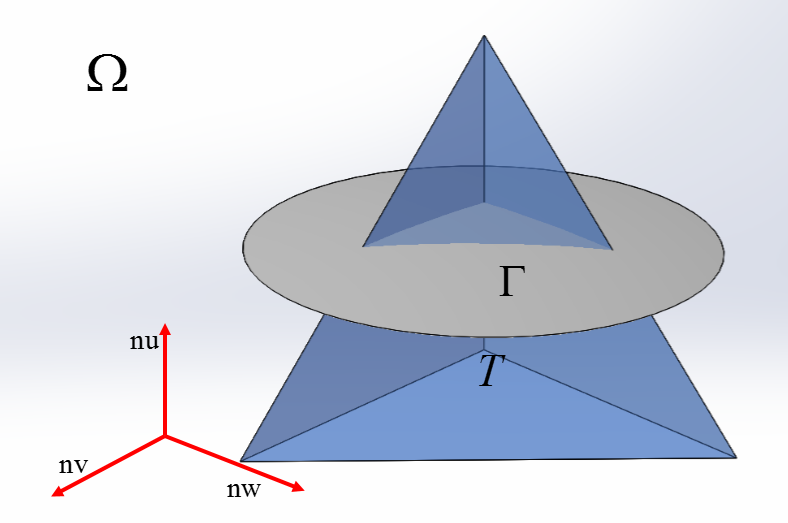
Figure 1: Intersection of surface and tetrahedron

We describe the method briefly as follows. As shown in Figure 1, suppose we choose an appropriate rectangular coordinate system $\{x_{0},\{{\boldsymbol{\mathrm{nu}},\boldsymbol{\mathrm{nv}},\boldsymbol{\mathrm{nw}}}\}\}$ so that $T$ is contained in a rectangular parallelepiped unit, i.e.,

(22) $$T\subset\left\{\mathrm{x}_{0}+r\mathbf{nu}+s\mathbf{nv}+t\mathbf{nw}\mid r\in(0,a),s\in(0,b),t\in(0,c)\right\}.$$

Then we directly use a projection method to calculate the surface integral in the parametric domain, i.e.,

(23) $$I=\int_{F_{T}}u(\mathrm{x})\mathrm{d}S=\int_{0}^{c}\int_{0}^{b}\tilde{g}(s,t)\mathrm{d}s\mathrm{d}t=\int_{0}^{c}{\color[rgb]{0,0,0}{\tilde{h}(t)\mathrm{d}t,}}$$

where

(24) $$\begin{array}[]{l}\tilde{g}(s,t):=\left\{\begin{array}[]{ll}u\left(r_{0},s,t\right)&\frac{\left|\nabla\varphi\left(\mathrm{x}\left(r_{0},s,t\right)\right)\right|}{\left|\mathbf{n}\mathbf{u}\cdot\nabla\varphi\left(\mathrm{x}\left(r_{0},s,t\right)\right)\right|},\quad\text{ if }\exists r_{0},\text{ s.t. }\mathrm{x}\left(r_{0},s,t\right)\in F_{T},\\ 0,&\text{ otherwise;}\end{array}\right.\\ \tilde{h}(t):=\int_{0}^{b}\tilde{g}(s,t)\mathrm{d}s.\end{array}$$

Although the approach looks straightforward, there are difficulties in implementation. First, the integrand is discontinuous and we need search for the discontinuity points in each interval of integration. Second, the integrand might be singular if the normal $\mathbf{nu}$ is not chosen properly so that it is tangential to $F_{T}$ at some point. In this case, we need detect the singular points in the integration and change coordinates to avoid them. More details are referred to [16]. Other approaches for high order quadratures on curved surfaces can be found in [53, 67].

4.2 The algebraic problem

Suppose the finite element basis functions of $W_{h}$ are given by $\{\phi_{1},\phi_{2},\cdots,\phi_{M}\}$. We express the solution of (17) as $\hat{u}_{h}=\sum_{i=1}^{M}u_{i}\phi_{i}$. Let $\mathbf{u}=(u_{1},u_{2},\cdots,u_{M})$. When $c$ is a constant, the algebraic system of the discrete Laplace-Beltrami problem (17) can be written as,

(25) $$(A+cB)\mathbf{u}=\mathbf{f},$$

where the elements of the matrices $A$ and $B$ are given by

$$a_{ij}=a(\phi_{i},\phi_{j}),\quad b_{ij}=(\phi_{i},\phi_{j})_{\Gamma},\qquad i,j=1,\cdots,M,$$

and $\mathbf{f}=\{\left(f,\phi_{i}\right)_{\Gamma},i=1,\cdots,M\}$. Similarly, the algebraic problem corresponding to (19) can be written as,

(26) $$A\mathbf{u}=\lambda B\mathbf{u}.$$

When the conditions of Lemma 3.1 are not satisfied, neither the algebraic problem (25) nor the generalized eigenvalue problem (26) are well defined. For the algebraic problems, we introduce a new equivalent condition of Lemma 3.1.

Lemma 4.1.

The condition of Lemma 3.1 holds if and only if $B$ is nonsingular.

Proof.

Notice the equivalence between the condition (iv) in Lemma 3.1 and the definition of $B$, the conclusion can be drawn immediately.

When the condition of Lemma 4.1 holds, we easily see that $\operatorname{rank}(B)=\operatorname{dim}(W_{h})=\operatorname{rank}(A)+1={\color[rgb]{0,0,0}{\operatorname{rank}(A+cB)}}$ when $c$ is not an eigenvalue of (26). In this case, the algebra problem $(A+cB)\mathbf{u}=\mathbf{f}$ has a unique solution. Meanwhile, since the matrix $B$ is invertible, $A\mathbf{u}=\lambda B\mathbf{u}$ can be understand in a usual way,

(27) $$B^{-1}A\mathbf{u}=\lambda\mathbf{u}.$$

When the condition of Lemma 4.1 is not satisfied, the algebra problem $(A+cB)\mathbf{u}=\mathbf{f}$ may have multiple solutions even when $c>0$. However, all of the solutions correspond to the same trace $\sum_{i=1}^{M}u_{i}\phi_{i}|_{\Gamma}$ on $\Gamma$. Thus we can still obtain an approximate solution for the Laplace-Beltrami equation whenever we find a solution of (25). When $B$ is singular, there is more trouble for the eigenvalue problem, as discussed in Section 3.3. The problem $A\mathbf{u}=\lambda B\mathbf{u}$ is not well defined since both $A$ and $B$ are singular. One can show that there exists a non-zero vector $\mathbf{u}$ such that $A\mathbf{u}=\mathbf{0}=B\mathbf{u}$. In this case, any $\lambda\in\mathbb{R}$ satisfies the equation. Moreover, we cannot get the multiplicity of a specific eigenvalue correctly. To focus on the eigenvalues we are interested in, we need study the “true eigenvalues” of the generalized eigenvalue problem (26).

We recall some standard definitions for the finite eigenvalues of singular generalized eigenvalue problems(which means that $\mathrm{det}(A-\lambda B)\equiv 0$ for all $\lambda\in\mathbb{C}$) [21]. We first introduce a definition for the normal rank of two matrices $A$ and $B$.

Definition 4.1 (normal rank).

For any two matrices $A$ and $B$, the normal rank $\operatorname{nrank}(A,B)$ is defined as

(28) $$\operatorname{nrank}(A,B):=\max_{\beta\in\mathbb{C}}\operatorname{rank}(A-\beta B)$$

Definition 4.2 (finite eigenvalues).

A number $\lambda_{k}\in\mathbb{C}$ satisfying

(29) $$\operatorname{rank}\left(A-\lambda_{k}B\right)<\operatorname{nrank}(A,B)$$

is called a finite eigenvalue of the generalized eigenvalue problem (26).

Notice that both $A$ and $B$ in (26) are semi-positive symmetric matrices in our problem, we can consider only the finite eigenvalues in $\mathbb{R}$. In addition, when $B$ is invertible, we have $\operatorname{nrank}(A,B)=\operatorname{rank}(B)$ and the above defined finite eigenvalues coincide with the standard eigenvalues of (27).

We will show that the finite eigenvalues of (26) are exactly the same as the true eigenvalues of (19). Furthermore, considering the multiplicity of eigenvalues, they are exactly the eigenvalues of (18).

Let us assume that $\{\phi_{1}|_{\Gamma},\phi_{2}|_{\Gamma},\cdots,\phi_{M-K}|_{\Gamma}\}$ is a set of linearly independent basis functions of $V_{h}$, where $K=\operatorname{dim}W_{h}-\operatorname{dim}V_{h}$. We define the stiffness matrix and mass matrix in $\mathbb{R}^{(M-K)\times(M-K)}$ as

(30) $$\tilde{A}=\big{(}a(\phi_{i},\phi_{j})\big{)},\quad\tilde{B}=\big{(}(\phi_{i},\phi_{j})_{\Gamma}\big{)},\quad 1\leq i,j\leq M-K.$$

Then, the algebraic eigenvalue problem corresponding to (18) is

(31) $$\tilde{A}\mathbf{x}=\lambda\tilde{B}\mathbf{x}.$$

It is easy to see that the eigenvalues of this problem are the true eigenvalues of (19). Further, it is a well-posed approximation of the problem (4) while considering the multiplicity of eigenvalues as introduced in [32]. The following theorem gives the relation between the regular generalized eigenvalue problem (31) and the singular generalized eigenvalue problem (26).

Theorem 4.1.

Suppose that $\{\phi_{1},\cdots,\phi_{M-K-1},\phi_{M-K},\cdots,\phi_{M}\}$ forms a basis of the finite element space $W_{h}$ and $\{\phi_{1}|_{\Gamma},\cdots,\phi_{M-K}|_{\Gamma}\}$ forms a basis of $V_{h}$. Then the generalized eigenvalue problem (26) and (31) share the same finite eigenvalues.

Proof.

By the assumption of the theorem, we easily know that there exist a matrix $C:=\{c_{i,j},i=1,\cdots,K,j=1,\cdots,M-K$}, satisfying

(32) $$\left(\begin{array}[]{c}\phi_{M-K+1}|_{\Gamma}\\ \phi_{M-K+2}|_{\Gamma}\\ \vdots\\ \phi_{M}|_{\Gamma}\end{array}\right)=\left(\begin{array}[]{cccc}c_{1,1}&c_{1,2}&\cdots&c_{1,M-K}\\ c_{2,1}&c_{2,2}&\cdots&c_{2,M-K}\\ \vdots&\vdots&\ddots&\vdots\\ c_{K,1}&c_{\mathrm{K},2}&\cdots&c_{K,\mathrm{~{}M-K}}\end{array}\right)\left(\begin{array}[]{c}\phi_{1}|_{\Gamma}\\ \phi_{2}|_{\Gamma}\\ \vdots\\ \phi_{M-K}|_{\Gamma}\end{array}\right).$$

We write

$$A=\left(\begin{array}[]{cc}A_{11}&A_{12}\\ A_{21}&A_{22}\end{array}\right),B=\left(\begin{array}[]{cc}B_{11}&B_{12}\\ B_{21}&B_{22}\end{array}\right)$$

where $A_{11}=\tilde{A},B_{11}=\tilde{B}$. Define a transformation matrix

$$P=\left(\begin{array}[]{cc}I_{(M-K)\times(M-K)}&0\\ -C&I_{K\times K}\end{array}\right)$$

where $I_{k\times k}$ is the $k\times k$ unit matrix for some positive integer $k$. From (32) and the definitions of $A$ and $B$, one derives

$$\bar{A}:=PAP^{T}=\left(\begin{array}[]{cc}A_{11}&0\\ 0&0\end{array}\right),\bar{B}:=PBP^{T}=\left(\begin{array}[]{cc}B_{11}&0\\ 0&0\end{array}\right).$$

Since $P$ is invertible, simple arguments in linear algebra indicate that

$$\operatorname{rank}(A-\lambda B)=\operatorname{rank}(\bar{A}-\lambda\bar{B})=\operatorname{rank}(A_{11}-\lambda B_{11})=\operatorname{rank}(\tilde{A}-\lambda\tilde{B}),\quad\forall\lambda\in\mathbb{R}.$$

The fact $\operatorname{rank}(B)=\operatorname{rank}(\tilde{B})$ reveals that

(33) $$\operatorname{rank}(A-\lambda B)<\operatorname{rank}(B)\Leftrightarrow\operatorname{rank}(\tilde{A}-\lambda\tilde{B})<\operatorname{rank}(\tilde{B}).$$

By the definition of the stiffness matrix $A$ and the mass matrix $B$ of the trace finite element method, we can easily check that $\operatorname{nrank}(A,B)=\operatorname{rank}(B)$ and also $\operatorname{nrank}(\tilde{A},\tilde{B})=\operatorname{rank}(\tilde{B})$. This together with (33) implies the conclusion of the theorem.

By the above theorem, to obtain the true eigenvalues of the discrete problem (19) with their correct multiplicity, we can compute the finite eigenvalues of the generalized (algebraic) eigenvalue problem (26). There exist many algorithms in literature to solve a singular generalized eigenvalue problem [71, 73, 22, 52]. Recently, an efficient and robust algorithm has been developed by a rank-completing perturbation technique in [40]. In this method, one constructs a perturbation of the singular problem which shares the same finite eigenvalues with the original problem. Then, the finite eigenvalues can be selected by using the left and right eigenvectors of the perturbed problem to satisfy certain conditions. In our experiments we use the algorithm in [40] to solve the singular generalized eigenvalue problem (26). More details are referred to [40].

Remark 4.1.

For the standard trace FEMs on discrete surfaces, we could use the same idea to construct and solve the corresponding generalized eigenvalue problems. We will present some comparisons in our numerical experiments in Section 6.

5 Error analysis

In this section, we will present error analysis for the trace finite element method introduced in the previous sections. Since there is no geometric error induced by the discretization of the surface, the analysis is simpler than that for the standard trace finite element methods [60]. In the analysis, we ignore the errors due to numerical quadratures for simplicity.

5.1 The Laplace-Beltrami equation

We first introduce some notations. Let $d(x)$ be a signed distance function of $\Gamma$. Then the unit normal vector of $\Gamma$ is given by

(34) $$\mathbf{n}({x}):=\nabla d({x}),\quad\forall{x}\in\mathcal{N}_{\delta}$$

The closest point projection operator $\mathbf{p}(x)$ is defined as

(35) $$\mathbf{p}({x})={x}-d({x})\mathbf{n}({x}),\quad\forall{x}\in\mathcal{N}_{\delta}.$$

For a smooth surface with bounded mean curvature, we can choose $\delta$ small enough to make the projection uniquely defined for all ${x}\in\mathcal{N}_{\delta}$. Given a function $v:\Gamma\rightarrow\mathbb{R}$, we define its natural extension $v^{e}$ in $\mathcal{N}_{\delta}$ as,

(36) $$v^{e}({x})={v}\left(\mathbf{p}({x})\right)={v}({x}-d({x})\nabla d({x})),\quad\forall{x}\in\mathcal{N}_{\delta}.$$

Suppose that the mesh size $h$ is small enough so that $\omega_{h}\subset\mathcal{N}_{\delta}.$ Denote by $\Pi_{h}:C\left({\omega_{h}}\right)\rightarrow W_{h}$ be the standard Lagrange interpolation operator of degree up to $k$ in the bulk region. In the following, we use $x\lesssim y$ to represent $x\leq c_{0}y$ for some constant $c_{0}$ independent of the mesh size $h$. In the analysis, we assume $c\geq 0$ in the problem (1).

The following interpolation result is standard in the finite element theory (e.g. [14]).

Lemma 5.1.

Let $0\leq m\leq k+1$ and $\hat{v}\in H^{k+1}(\omega_{h})$, we have

(37) $$\|\hat{v}-\Pi_{h}\hat{v}\|_{H^{m}(\omega_{h})}\lesssim h^{k+1-m}\|\hat{v}\|_{H^{k+1}(\omega_{h})}.$$

This inequality also holds elementwisely, i.e. for any $T\in\mathcal{T}_{\Gamma}$,

(38) $$\|\hat{v}-\Pi_{h}\hat{v}\|_{H^{m}(T)}\lesssim h^{k+1-m}\|\hat{v}\|_{H^{k+1}(T)}.$$

The next lemma is a modified version of the trace inequality.

Lemma 5.2.

Suppose that the surface $\Gamma$ is smooth and $\max\limits_{x\in\Gamma}(|\kappa_{1}(x)|+|\kappa_{2}(x)|)<C_{\kappa}$, where $\kappa_{1}$ and $\kappa_{2}$ represent two principal curvatures. Let $F_{T}$ be the intersection between $\Gamma$ and an element $T$, then

(39) $$\|w\|_{0,F_{T}}^{2}\lesssim h^{-1}\|w\|^{2}_{0,T}+h\|w\|^{2}_{1,T},$$

holds for all $w\in H^{1}(T)$ when $h$ is smaller than a positive number $c_{0}(C_{\kappa})$.

Proof.

We first map the element $T$ by an affine mapping to a reference element $\tilde{T}$ and denote by $\tilde{F}_{T}$ the image of $F_{T}$. Assume $\tilde{F}_{T}$ divides $\tilde{T}$ into two subsets $\tilde{T}_{1}$ and $\tilde{T}_{2}$ where $T_{1}$ is shape regular. The coordinates in the reference domain are denoted as $(\xi_{1},\xi_{2},\xi_{3})$. Let $\boldsymbol{n}=(n_{\xi_{1}},n_{\xi_{2}},n_{\xi_{3}})$ be the outward unit normal of the boundary of $\tilde{T}_{1}$. Without loss of generality, we could assume that there is at least one point on $\tilde{F}_{T}$ such that $\boldsymbol{n}=(0,0,1)^{T}$. This can be done by a simple rotation of $\tilde{T}$ if the condition does not hold. Since the size of $\tilde{T}$ is unit, the sum of the principle curvatures of $\tilde{F}_{T}$ should be smaller than $C_{\kappa}h$. Then we have the out normal $|\boldsymbol{n}-(0,0,1)^{T}|\leq C_{\kappa}h$ on $\tilde{F}_{T}$. It is easy to see that we have $n_{\xi_{3}}\geq 1-C_{\kappa}h$.

Then, by the divergence theorem, we have

(40) $$2\int_{\tilde{T}_{1}}w\frac{\partial w}{\partial\xi_{3}}\mathrm{d}V =\int_{\tilde{T}_{1}}\operatorname{div}\left(0,0,w^{2}\right)^{T}\mathrm{d}V=\int_{\partial\tilde{T}_{1}}\boldsymbol{n}\cdot\left(0,0,w^{2}\right)^{T}\mathrm{d}S$$

$$\geq(1-C_{\kappa}h)\int_{\tilde{F}_{T}}w^{2}\mathrm{~{}d}S+\int_{\partial\tilde{T}_{1}\backslash\tilde{F_{T}}}n_{\xi_{3}}w^{2}\mathrm{~{}d}S.$$

From Cauchy-Schwarz’ inequality and the well-known trace inequality,

(41) $$\|w\|_{0,\partial\tilde{T}}^{2}\leq C\|w\|_{0,\tilde{T}}\|w\|_{1,\tilde{T}},\quad\forall w\in H^{1}(\tilde{T}),$$

one derives

(42) $$(1-C_{\kappa}h)\|w\|_{0,\tilde{F}_{T}}^{2} \leq 2\|w\|_{0,\tilde{T}_{1}}\|w\|_{1,\tilde{T}_{1}}+\|w\|_{0,\partial\tilde{T}_{1}\backslash\tilde{F_{T}}}^{2}$$

$$\leq 2\|w\|_{0,\tilde{T}_{1}}\|w\|_{1,\tilde{T_{1}}}+\|w\|_{0,\partial\tilde{T}}^{2}\leq C\|w\|_{0,\tilde{T}}\|w\|_{1,\tilde{T}}$$

$$\leq\frac{C}{2}(\|w\|_{0,\tilde{T}}^{2}+\|w\|_{1,\tilde{T}}^{2}).$$

One could easily choose a small $h$ such that $1>1-C_{\kappa}h\geq C_{0}>0$. Then the result of the lemma follows by a standard scaling argument since $T$ is shape regular.

The following lemma gives some estimates on the extensions.

Lemma 5.3.

Under the condition of Lemma 5.2, suppose $u\in H^{k+1}(\Gamma)$ with $k\geq 1$ and $m=0,1$, then we have

(43) $$\|u^{e}\|_{H^{m}(\mathcal{N}_{\delta})}\lesssim h^{1/2}\|u\|_{H^{m}(\Gamma)},$$

and

(44) $$\|u-\Pi_{h}u^{e}\|_{H^{m}(\Gamma)}\lesssim h^{k+1/2-m}\|u^{e}\|_{H^{k+1}(\omega_{h})}.$$

Proof.

Resort to (3.17) and (3.18) in [60],

(45) $$\left\|u^{e}\right\|_{L^{2}\left(\mathcal{N}_{\delta}\right)}\lesssim\sqrt{h}\|u\|_{L^{2}(\Gamma)},\qquad\left\|\nabla u^{e}\right\|_{L^{2}\left(\mathcal{N}_{\delta}\right)}\lesssim\sqrt{h}\|\nabla u\|_{L^{2}(\Gamma)}.$$

By the two equations, we easily get

$$\left\|u^{e}\right\|^{2}_{L^{2}\left(\mathcal{N}_{\delta}\right)}+\left\|\nabla u^{e}\right\|^{2}_{L^{2}\left(\mathcal{N}_{\delta}\right)}\lesssim{h}\|u\|^{2}_{L^{2}(\Gamma)}+{h}\|\nabla_{\Gamma}u\|^{2}_{L^{2}(\Gamma)}$$

This completes the proof of (43). Recall lemma 5.2,

(46) $$\|w\|_{L_{2}(F_{T})}\lesssim h^{-\frac{1}{2}}\|w\|_{L_{2}(T)}+h^{\frac{1}{2}}\left\|\nabla_{\Gamma}w\right\|_{L_{2}(T)},\quad\forall w\in H^{1}(T).$$

Together with lemma 5.1, we write

$$\begin{split}\left\|u-\Pi_{T}u^{e}\right\|_{L^{2}(F_{T})}\lesssim&h^{-1/2}\left\|u^{e}-\Pi_{T}u^{e}\right\|_{L^{2}(T)}+h^{1/2}\left\|\nabla(u^{e}-\Pi_{T}u^{e})\right\|_{L^{2}(T)}\\ \lesssim&h^{k+1/2}\left\|u^{e}\right\|_{H^{k+1}(T)}.\end{split}$$

Similar estimates follow similarly for the semi-$H^{1}$ norm,

$$\begin{split}\left\|\nabla(u-\Pi_{T}u^{e})\right\|_{L^{2}(F_{T})}\lesssim&h^{-1/2}\left\|\nabla(u^{e}-\Pi_{T}u^{e})\right\|_{L^{2}(T)}+h^{1/2}\left\|\nabla^{2}(u^{e}-\Pi_{T}u^{e})\right\|_{L^{2}(T)}\\ \lesssim&h^{k-1/2}\left\|u^{e}\right\|_{H^{k+1}(T)}.\end{split}$$

The assertion (44) follows by summation of the above equations for all $T\in\omega_{h}$.

Lemma 5.4 (Approximation in $H^{1}$ norm).

Under the condition of Lemma 5.2, suppose that ${u}\in$ $H^{k+1}(\Gamma)$ with $k\geq 1$, then we have

(47) $$\inf_{v_{h}\in{V}_{h}}\left\|{u}-v_{h}\right\|_{H^{1}(\Gamma)}\lesssim h^{k}\|{u}\|_{H^{k+1}(\Gamma)}.$$

Proof.

Applying Lemma 5.3 directly yields

$$\begin{split}\inf_{v_{h}\in{V}_{h}}\left\|{u}-v_{h}\right\|_{H^{1}(\Gamma)}&\lesssim\|u-\Pi_{h}u^{e}\|_{H^{1}(\Gamma)}\lesssim h^{k-1/2}\|u^{e}\|_{H^{k+1}(\omega_{h})}\\ &\lesssim h^{k-1/2}\|u^{e}\|_{H^{k+1}(\mathcal{N}_{\delta})}\lesssim h^{k}\|u\|_{H^{k+1}(\Gamma)}.\end{split}$$

Theorem 5.1 (A-priori error estimates).

Suppose the condition of Lemma 5.2 holds and the solution $u$ of the problem (1) with $c\geq 0$ is in $H^{k+1}(\Gamma)$. Let $u_{h}\in{V}_{h}$ be the solution of the finite element discretization (16). We assume both $u$ and $u_{h}$ satisfy the zero-average condition on $\Gamma$ when $c=0$. Then we have

$$\left\|u-u_{h}\right\|_{L_{2}(\Gamma)}+h\left\|\nabla_{\Gamma}\left(u-u_{h}\right)\right\|_{L_{2}(\Gamma)}\lesssim h^{k+1}\|{u}\|_{H^{k+1}(\Gamma)}.$$

Proof.

We only prove the theorem when $c>0$. When $c=0$, the proof is similar with the assumption that $\int_{\Gamma}uds=\int_{\Gamma}u_{h}ds=0$.

Define $\hat{a}(u,v):=a(u,v)+(cu,v)_{\Gamma}$. Take $v=v_{h}$ in (2) and then subtract (16), arrive at

$$\hat{a}(u-u_{h},v_{h})=0,\quad\forall v_{h}\in V_{h}(\Gamma).$$

According to the continuity and ellipticity of bilinear operator $\hat{a}$,

$$\begin{split}\left\|u-u_{h}\right\|^{2}_{H^{1}(\Gamma)}&\lesssim\hat{a}(u-u_{h},u-u_{h})\\ &=\hat{a}(u-u_{h},u-v_{h})+\hat{a}(u-u_{h},v_{h}-u_{h})\\ &\lesssim\left\|u-u_{h}\right\|_{H^{1}(\Gamma)}\left\|u-v_{h}\right\|_{H^{1}(\Gamma)}\end{split}$$

then we have

(48) $$\left\|\nabla_{\Gamma}\left(u-u_{h}\right)\right\|_{L_{2}(\Gamma)}\leq\left\|u-u_{h}\right\|_{H^{1}}\lesssim\left\|u-v_{h}\right\|_{H^{1}}\\ \lesssim h^{k}\|{u}\|_{H^{k+1}(\Gamma)}$$

Next, we use the Aubin-Nitsche duality technique to estimate the $L_{2}$ error. We now consider an auxiliary problem,

(49) $${z}\in H^{1}(\Gamma):\quad\hat{a}(z,w)=\int_{\Gamma}\left({u}-u_{h}\right)w\quad\forall w\in H^{1}(\Gamma)$$

and its finite element approximation problem,

(50) $${z_{h}}\in V_{h}(\Gamma):\quad\hat{a}(z_{h},w_{h})=\int_{\Gamma}\left({u}-u_{h}\right)w_{h}\quad\forall w_{h}\in V_{h}.$$

Take $w=u-u_{h}$ in (49),

$$\begin{split}\left\|u-u_{h}\right\|^{2}_{L^{2}}&=\hat{a}(z,u-u_{h})=\hat{a}(z-z_{h},u-u_{h})\\ &\lesssim\left\|z-z_{h}\right\|_{H^{1}(\Gamma)}\left\|u-u_{h}\right\|_{H^{1}(\Gamma)}\\ &\lesssim h^{k+1}\left\|u-u_{h}\right\|_{L^{2}}\left\|u\right\|_{H^{k+1}(\Gamma)},\\ \end{split}$$

where in the last inequality we have used $H^{1}$ error estimate (48) and the regularity property $\|z\|_{H^{2}(\Gamma)}\leq\left\|u-u_{h}\right\|_{L^{2}}$ for the problem (49). This completes the proof.

5.2 The Laplace-Beltrami eigenvalue problem

For the error estimate for the Laplace-Beltrami eigenvalue problem, we adopt the standard approach using the spectral approximation theory for compact operators [2, 7, 70]. This is based on the error analysis for the Laplace-Beltrami equation in the previous subsection.

We first introduce some operators as in [2, 70] for the weak formula of the Laplace-Beltrami equations. In this subsection, we consider only the nontrivial eigenvalues. We denote the function space

$$H^{1}_{c}(\Gamma)=\{v\in H^{1}(\Gamma)\ |\ \int_{\Gamma}vds=0.\}$$

and

$$L_{c}^{2}(\Gamma)=\{v\in L^{2}(\Gamma)\ |\ \int_{\Gamma}vds=0.\}$$

Then an operator $T:L_{c}^{2}(\Gamma)\mapsto L_{c}^{2}(\Gamma)$ is defined as follows. For any $f\in L_{c}^{2}(\Gamma)$, $Tf\in H^{1}_{c}(\Gamma)\subset L_{c}^{2}(\Gamma)$ is a function satisfies

(51) $$a(Tf,v)=(f,v)_{\Gamma},\qquad\forall v\in H^{1}_{c}(\Gamma).$$

This is the Laplace-Beltrami equation (2) (with $c=0$). It is easy to know that the problem is well-defined and $\|Tf\|_{H^{1}}\leq\|f\|_{L^{2}}$. Then the Sobolev embedding theorem implies that $T:L_{c}^{2}(\Gamma)\mapsto L_{c}^{2}(\Gamma)$ is compact. It is easy to check that the operator $T$ is also self-adjoint:

$$(Tf,g)_{\Gamma}=(g,Tf)_{\Gamma}=a(Tg,Tf)=a(Tf,Tg)=(f,Tg)_{\Gamma}.$$

Furthermore, if $\lambda$ is a nonzero eigenvalue of the Laplace-Beltrami eigenvalue problem (5), then $\lambda^{-1}$ is the eigenvalue of $T$, corresponding to the same eigenfunctions.

Denote by $V_{h,c}=V_{h}\cap H^{1}_{c}$, i.e. $V_{h,c}=\{v_{h}\in V_{h}:\int_{\Gamma}vds=0\}$. We can define a discrete operator $T_{h}:L_{c}^{2}(\Gamma)\mapsto L_{c}^{2}(\Gamma)$ analogously. For any $f\in L^{2}_{c}(\Gamma)$, $T_{h}f\in V_{h,c}\subset L_{c}^{2}(\Gamma)$ is determined by

(52) $$a(T_{h}f,v_{h})=(f,v_{h})_{\Gamma},\qquad\forall v_{h}\in V_{h,c}.$$

It is easy to see that $T_{h}f$ is the finite element solution of (16) with $c=0$. $T_{h}$ is a self-adjoint operator. If $\lambda_{h}$ is a nonzero eigenvalue of the problem (18), then $\lambda^{-1}_{h}$ is the eigenvalue of $T_{h}$. In addition, the error analysis in last subsection implies that

$$\|Tf-T_{h}f\|_{H^{1}}\leq Ch^{k}\|f\|_{k-1},$$

where we use the well-known regularity result that $\|u\|_{H^{k+1}}\lesssim\|f\|_{k-1}$ for the Laplace-Beltrami equation.

We have the following optimal error estimate for the trace finite element method for the eigenvalue problem.

Theorem 5.2.

Let $\lambda$ be a nonzero eigenvalue of the problem (5) with multiplicity $m$. Let $u_{i}$, $i=1,\cdots,m,$ be orthogonal eigenfunctions corresponding to $\lambda$. We suppose that $u_{i}\in H^{k+1}(\Gamma)$. Let $\lambda_{h,i},i=1,\cdots,m,$ be the solutions of the discrete problem (18) approximating to $\lambda$. Then we have the following error estimates

$$\left|\lambda-\hat{\lambda}_{h}\right|\lesssim h^{2k},$$

where $\hat{\lambda}_{h}=\frac{1}{m}\sum_{i=1}^{m}\lambda_{h,i}$.

Proof.

By the definition of the operators $T$ and $T_{h}$, we can apply the Babuska-Osborn theory. Denote $E=\text{span}\{u_{1},\cdots,u_{m}\}$. By Corollary 9.6. in [7], noticing that both $T$ and $T_{h}$ are self-adjoint, we obtain

$$|\lambda-\hat{\lambda}_{h}| \leq C\Big{(}\sup_{u\in E,\|u\|_{L^{2}(\Gamma)}=1}\inf_{v_{h}\in V_{h,c}}\|u-v_{h}\|_{H^{1}}\Big{)}^{2}$$

$$\leq C\Big{(}\sup_{u\in E,\|u\|_{L^{2}(\Gamma)}=1}h^{k}\|u\|_{H^{k+1}}\Big{)}^{2}\lesssim h^{2k}.$$

Remark 5.1.

By definition, the error estimate holds for the nonzero true eigenvalues of the embedded problems (9) and (19). In addition, error analysis for eigenfunctions can be done in a standard way [7], which is omitted here for simplicity.

6 Numerical experiments

In this section, we give some numerical examples to show the convergence behaviour of our method and compare with the original version of the trace finite element method. We implement the method in the finite element package DROPS [24] and use the package PHG[63] to do numerical integration on surfaces.

We first test our method by solving the Laplace-Beltrami equation (1).

Example 1. We solve the equation (1) on a unit sphere $\Gamma$:

$$\Gamma=\left\{x\in\mathbb{R}^{2}\ |\ \|x\|_{2}=1\right\}$$

which is contained in $\Omega:=[-2,2]^{3}$ and implicitly presented by the zero level of a function $\operatorname{\varphi}(x)=\|x\|_{2}-1$. We set $c=1$ and the right hand side term is given by $f(x)=\left(3x_{1}^{2}x_{2}-x_{2}^{3}\right).$ The solution of the equation is explicitly given by

$$u(x)=\frac{|x|^{2}}{12+|x|^{2}}\left(3x_{1}^{2}x_{2}-x_{2}^{3}\right),\quad x\in\Gamma.$$

For the triangulation we partition $\Omega$ uniformly into $N^{3}$ cubes and then each of them is subdivided into six tetrahedra. We solve the finite element problem (17) to get the numerical solution. In comparison, we also solve the problem (1) by using the isoparametric trace finite element method [37]. We compute the numerical errors in $L^{2}$ and $H^{1}$ norms. The experimental orders of convergence (EOC) are computed accordingly.

A numerical solution by our method is shown in Figure 2 ($k=2$, $N=64$). The numerical errors are given in Table 1 and 2. It is found that the geometrically consistent method (exTraceFEM) has optimal convergence rate, the same as the isoparametric method (isoTraceFEM). We can also see that the errors by the exTraceFEM is almost the same as that by the isoTraceFEM on a triangulation with the same mesh size when $k=1$(linear finite element case). This implies that the geometric error is neglectable for the low order method. However, for a higher order case ($k=2$), the numerical errors of exTraceFEM is much smaller than those of the isoparametric finite element method. This indicates that the effect of the geometric consistency is significant for high order finite element methods.

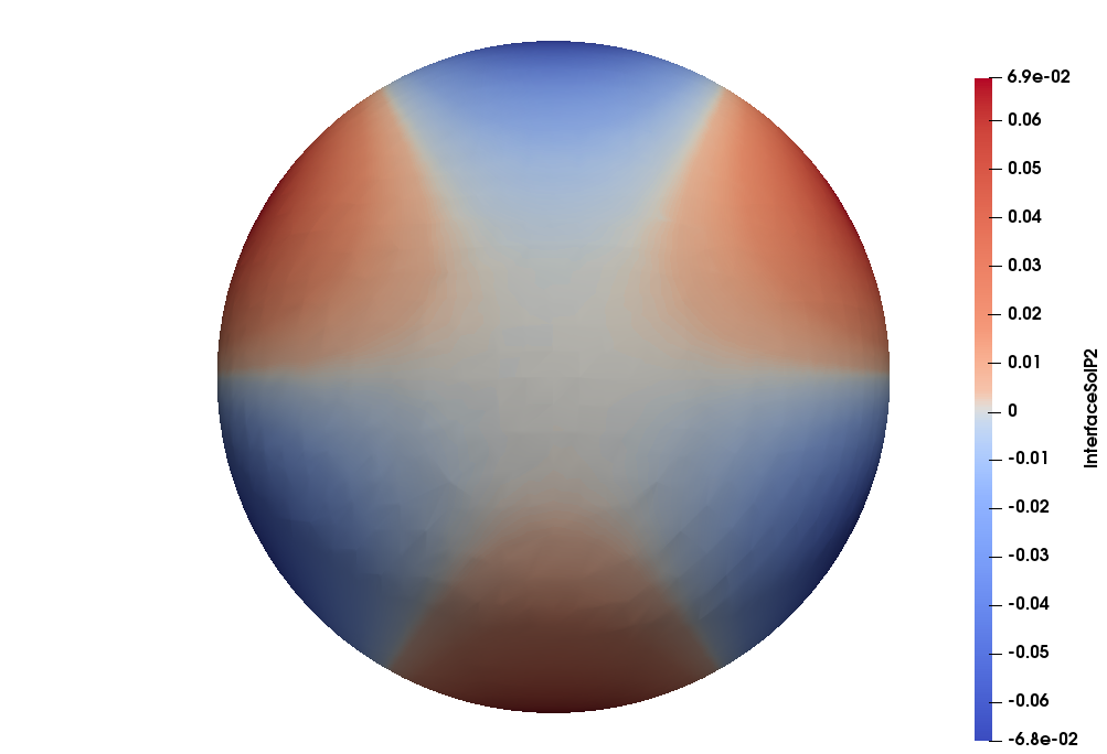
Figure 2: Numerical solution of the LB equation on a spherical surface

Table 1: Comparison of exTraceFEM and isoparametric TraceFEM (Example 1, $k=1$).

	isoTraceFEM				exTraceFEM
$N$	$E(H_{1})$	EOC	$E(L_{2})$	EOC	$E(H_{1})$	EOC	$E(L_{2})$	EOC
4	8.73E-1	-	4.88E-2	-	9.23E-1	-	6.68E-2	-
8	4.62E-1	0.92	1.99E-2	1.29	4.76E-1	0.96	2.05E-2	1.70
16	2.16E-1	1.10	5.32E-3	1.90	2.20E-1	1.11	5.12E-3	2.00
32	1.04E-1	1.05	1.38E-3	1.95	1.04E-1	1.08	1.30E-3	1.98
64	5.18E-2	1.00	3.33E-4	2.05	5.22E-2	0.99	3.13E-4	2.05

Table 2: Comparison of exTraceFEM and isoparametric TraceFEM (Example. 1, $k=2$).

	isoTraceFEM				exTraceFEM
$N$	$E(H_{1})$	EOC	$E(L_{2})$	EOC	$E(H_{1})$	EOC	$E(L_{2})$	EOC
4	2.52E-1	-	4.57E-2	-	1.70E-1	-	1.91E-1	-
8	4.26E-2	2.56	3.05E-3	3.91	1.08E-2	3.98	5.46E-4	8.45
16	9.94E-3	2.10	3.48E-4	3.13	2.56E-3	2.08	6.49E-5	3.07
32	2.61E-3	1.92	4.76E-5	2.87	6.61E-4	1.95	8.71E-6	2.90
64	6.55E-4	1.99	5.98E-6	2.99	1.64E-4	2.01	1.07E-6	3.03

We then present some numerical examples for the Laplace-Beltrami eigenvalue problem.

Example 2. In this example, we consider the eigenvalue problem (4) on the unit spherical surface. It is well known that the eigenvalues of the Laplace-Beltrami operator on the surface is given by

$$\lambda^{m}=\{m(m-1),m\geq 1\}$$

with a multiplicity of $p_{m}=2m-1$. We solve the problem (19) numerically. Meanwhile, we also solve the Laplace-Beltrami eigenvalue problem using a standard trace finite element method in [60].

We first compute the generalized eigenvalues of $A$ and $B$ using the Cholesky factorization method. The numerical results are shown in Table 3 and Table 4, which are respectively for the standard trace finite element method and the geometrically consistent method. For simplicity, we only show the first six eigenvalues. Here we choose $k=2$ and $N=32$. There are 2604 freedoms totally in the finite element space $W_{h}$. Our numerical results show that there are 448 false eigenvalues for the standard trace finite element method. This is actually because the dimension of $W_{h}$ is much larger than that of the space $V_{h}$ on a discretized surface $\Gamma_{h}$, as discussed in Section 3. Moreover, the geometrically consistent trace finite element method behaves much better than the standard trace finite element method in this case. There seems only one false eigenvalue $0.0069093$ which is close to the trivial eigenvalue $0$. This is consistent with our theoretical result in Lemma 3.1. In the same bulk finite element space $W_{h}$, $\operatorname{dim}$$(V_{h})$ of our method is much larger than that of the standard traceFEM, which indicates that the geometrically consistent method can generate much less false eigenvalues.

We then use the rank-completing perturbation algorithm [40] to compute the finite eigenvalues of the generalized eigenvalue problem (26). The numerical results by the standard method(traceFEM) and our method (exTraceFEM) ($k=2$ and $N=32$) are shown in Table 5 and Table 6, respectively. We can see that the false eigenvalues have been selected out as discussed in Section 4. Both the eigenvalues and their multiplicity are computed correctly. Similar to that for Laplace-Beltrami equation, the accuracy of the geometrically consistent method is much better than the standard method.

Table 3: traceFEM method when $k=2,N=32$

Eigenvalue	Numerical solutions
0	-1.8899201033073 -1.65160247438363 -1.60753159863045 $\cdots$ 1.146997797544159 1.173366051077160 1.404691246035232
2	2.000002341879660  2.000002341895009  2.000010968828590   2.008644495856585
6	6.000032528374658 6.000032528374662 6.000062692154771 6.000091817982969 6.000091817982981
12	12.000169159806013 12.000181120960798 12.000402418432977 12.000402418432987 12.000526221431546 12.000526221431546 12.000714928288357
20	20.000639807964866 20.000639807964877 20.001210428217536 20.001433468889189 20.002056244148882 20.002056244148889 20.002704995918332 20.002777886515734 20.002777886515734
30	30.001877620894145 30.001877620894149 30.003586778395437 30.003586778395444 30.005578378716464 30.006082304547288 30.007563415744823 30.007563415744837 30.008657097319883 30.008657097319894 30.009729163449663

Table 4: exTraceFEM method when $k=2,N=32$

Eigenvalue	Numerical solutions
0	-4.5702e-11 0.0069093
2	1.999999999970570 2.000000000028308 2.000000000051764
6	5.999999999933209 5.999999999940492 5.999999999994404 6.000000000001932 6.000000000036823
12	12.000011666430954 12.000020383250462 12.000024586245313 12.000024898829679 12.000024898928142 12.000034279424140 12.000034279500648
20	20.000121867977601 20.000121867991975 20.000131606614801 20.000188235821870 20.000188235928746 20.000189756600580 20.000204020147969 20.000235383589722 20.000235383594994
30	30.000514523042980 30.000534231291937 30.000534231297287 30.000635177166853 30.000635177208498 30.000771041561322 30.000771041608086 30.000836697770890 30.000836697819057 30.000856733024339 30.001005770449328

Table 5: traceFEM method when $k=2,N=32$

Eigenvalue	Numerical solutions
0	-6.44833099219222e-13
2	2.000002341879660 2.000002341895009 2.000010968828590
6	6.000032528374658 6.000032528374662 6.000062692154771 6.000091817982969 6.000091817982981
12	12.000169159806013 12.000181120960798 12.000402418432977 12.000402418432987 12.000526221431546 12.000526221431546 12.000714928288357
20	20.000639807964866 20.000639807964877 20.001210428217536 20.001433468889189 20.002056244148882 20.002056244148889 20.002704995918332 20.002777886515734 20.002777886515734
30	30.001877620894145 30.001877620894149 30.003586778395437 30.003586778395444 30.005578378716464 30.006082304547288 30.007563415744823 30.007563415744837 30.008657097319883 30.008657097319894 30.009729163449663

Table 6: exTraceFEM method when $k=2,N=32$

Eigenvalue	Numerical solutions
0	-4.5702e-11
2	1.999999999970570 2.000000000028308 2.000000000051764
6	5.999999999933209 5.999999999940492 5.999999999994404 6.000000000001932 6.000000000036823
12	12.000011666430954 12.000020383250462 12.000024586245313 12.000024898829679 12.000024898928142 12.000034279424140 12.000034279500648
20	20.000121867977601 20.000121867991975 20.000131606614801 20.000188235821870 20.000188235928746 20.000189756600580 20.000204020147969 20.000235383589722 20.000235383594994
30	30.000514523042980 30.000534231291937 30.000534231297287 30.000635177166853 30.000635177208498 30.000771041561322 30.000771041608086 30.000836697770890 30.000836697819057 30.000856733024339 30.001005770449328

We also compute the convergence rate of the eigenvalues. Let $\lambda^{m}(m=1,2,\cdots)$ be the m-th eigenvalue of the Laplace-Beltrami eigenvalue problem (4), and $p_{m}$ is the multiplicity of $\lambda^{m}$. We use $\{\lambda_{h,1}^{m},\lambda_{h,2}^{m},\cdots,\lambda_{h,p_{m}}^{m}\}$ to represent the eigenvalues approximating $\lambda^{m}$ by the discrete eigenvalue problem (18). The numerical error is calculated as,

(53) $$\operatorname{Error(\lambda^{m})}=\frac{1}{p_{m}}{\sum_{i=1}^{p_{m}}|\lambda^{m}-\lambda^{m}_{h,i}|}.$$

We compute the numerical errors for both the standard method and our method. The results for the cases $k=1$ and $k=2$ are shown in Figure 3 and Figure 4, respectively. We show the convergence for the first ten eigenvalues for simplicity. In general the experimental order of convergence is $2$ in the linear finite element case($k=1$) and the order is $4$ when $k=2$, except for the first a few eigenvalues, where the error is close to the machine accuracy. The optimal convergence orders agree with the error estimates in the previous section. In addition, some typical eigenfunctions are shown in Figure 5.

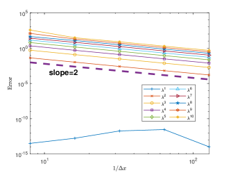
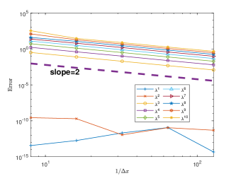
Figure 3: The errors of traceFEM (left) and exTraceFEM (right) for the Laplace-Beltrami eigenvalue problem(Example 2, k=1).

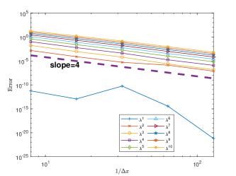
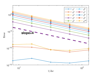
Figure 4: The errors of traceFEM (left) and exTraceFEM (right) for the Laplace-Beltrami eigenvalue problem(Example 2, k=1).

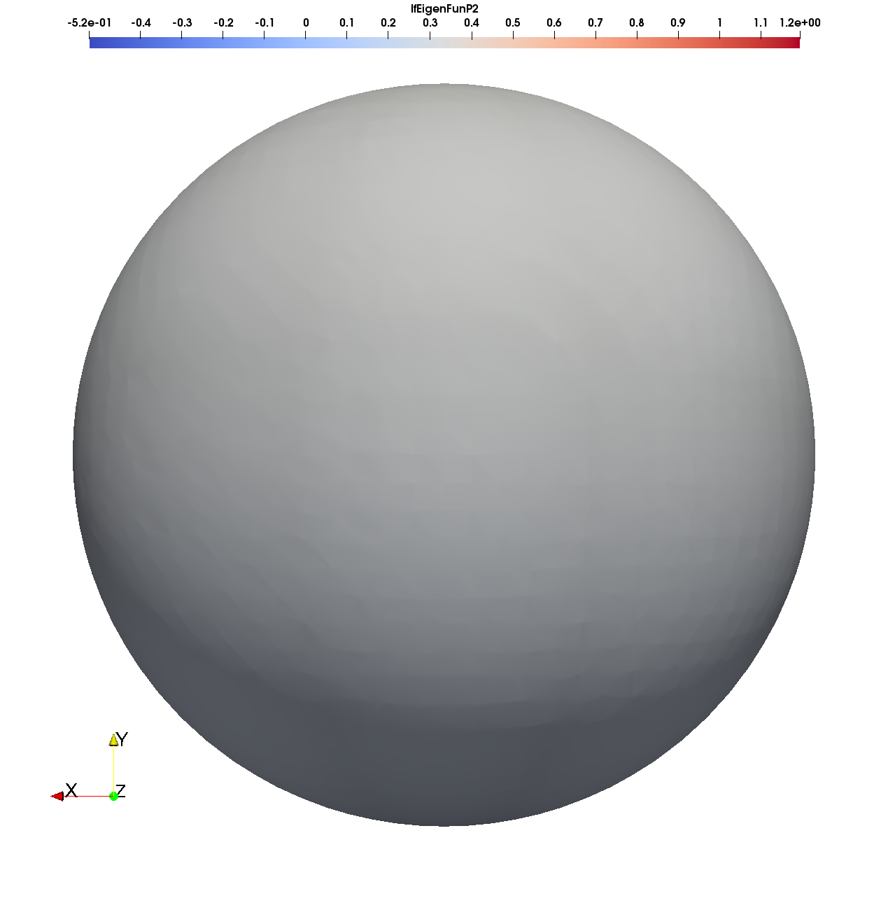
(a) $\lambda_{h,1}\approx 0$

(b) $\lambda_{h,2}\approx 2$

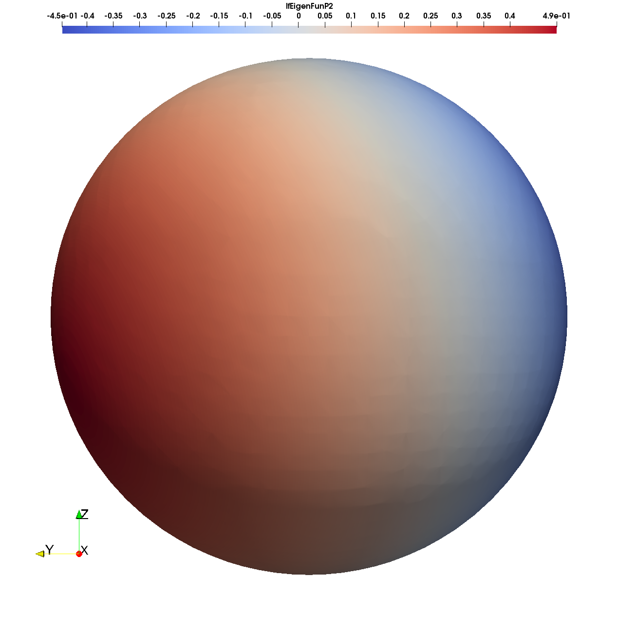
(c) $\lambda_{h,3}\approx 2$

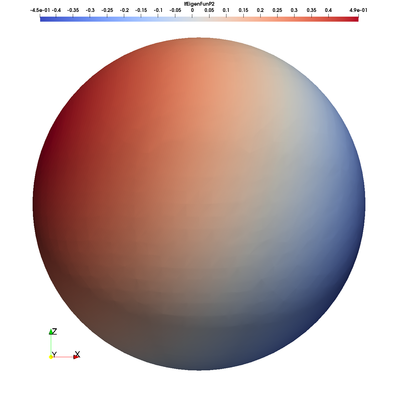
(d) $\lambda_{h,4}\approx 2$

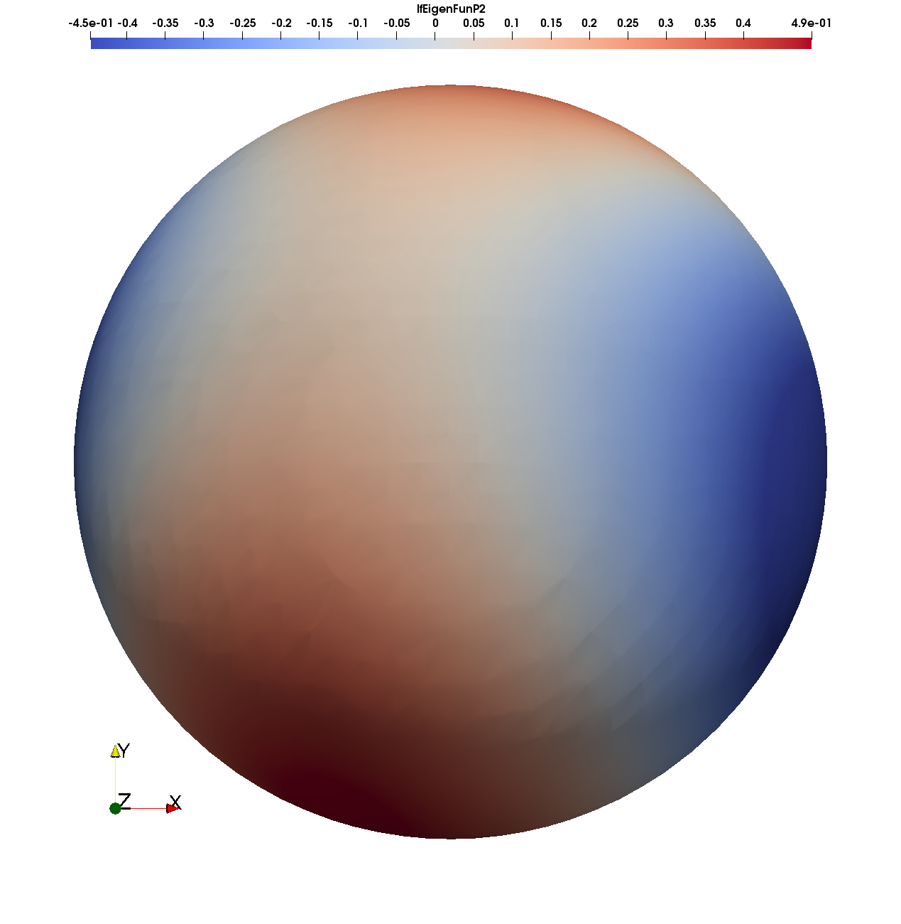
(e) $\lambda_{h,5}\approx 6$

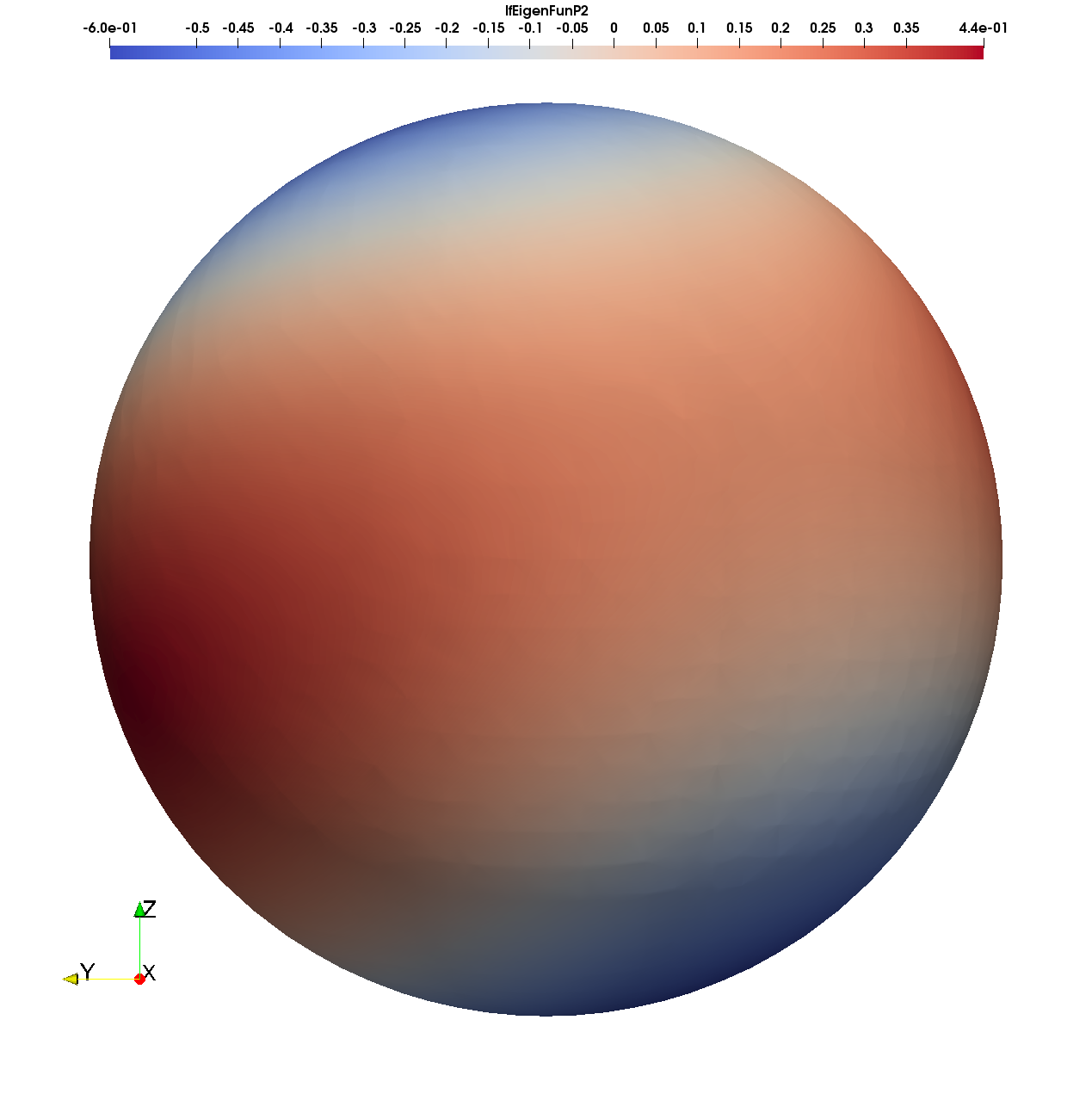
(f) $\lambda_{h,6}\approx 6$

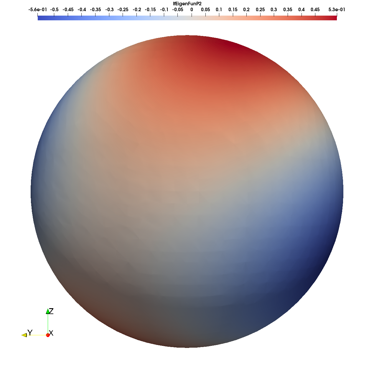
(g) $\lambda_{h,6}\approx 6$

(h) $\lambda_{h,7}\approx 6$

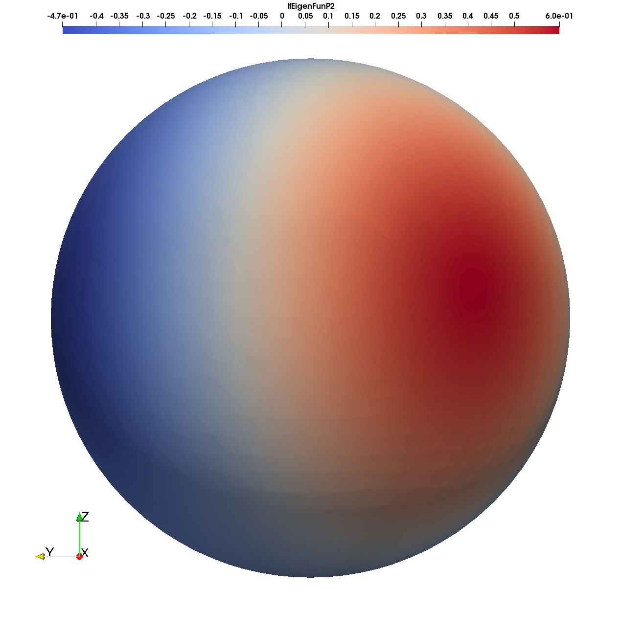
(i) $\lambda_{h,8}\approx 6$

Figure 5: The eigenfunctions for the Laplace-Beltrami operator on the unit spherical surface.

Example 3. In the last example, we solve the Laplace-Beltrami eigenvalue problem on a more general surface. Consider a tooth-shaped surface which is the zero level set of a function

(54) $$\varphi(x,y,z)=\frac{256\,x^{4}}{625}-\frac{16\,x^{2}}{25}+\frac{256\,y^{4}}{625}-\frac{16\,y^{2}}{25}+\frac{256\,z^{4}}{625}-\frac{16\,z^{2}}{25}.$$

By using our method, the set of true eigenvalues and the corresponding eigenfunctions on the surface are shown in Figure 6($k=1,N=32$). We show only the first six ones for simplicity. We can see that our method works well for this problem.

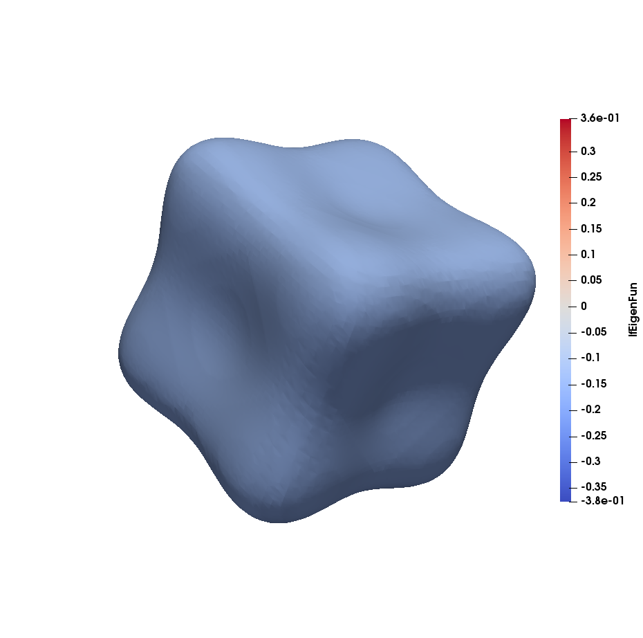
(a) $\lambda_{h,1}=9.0291211439e-12$

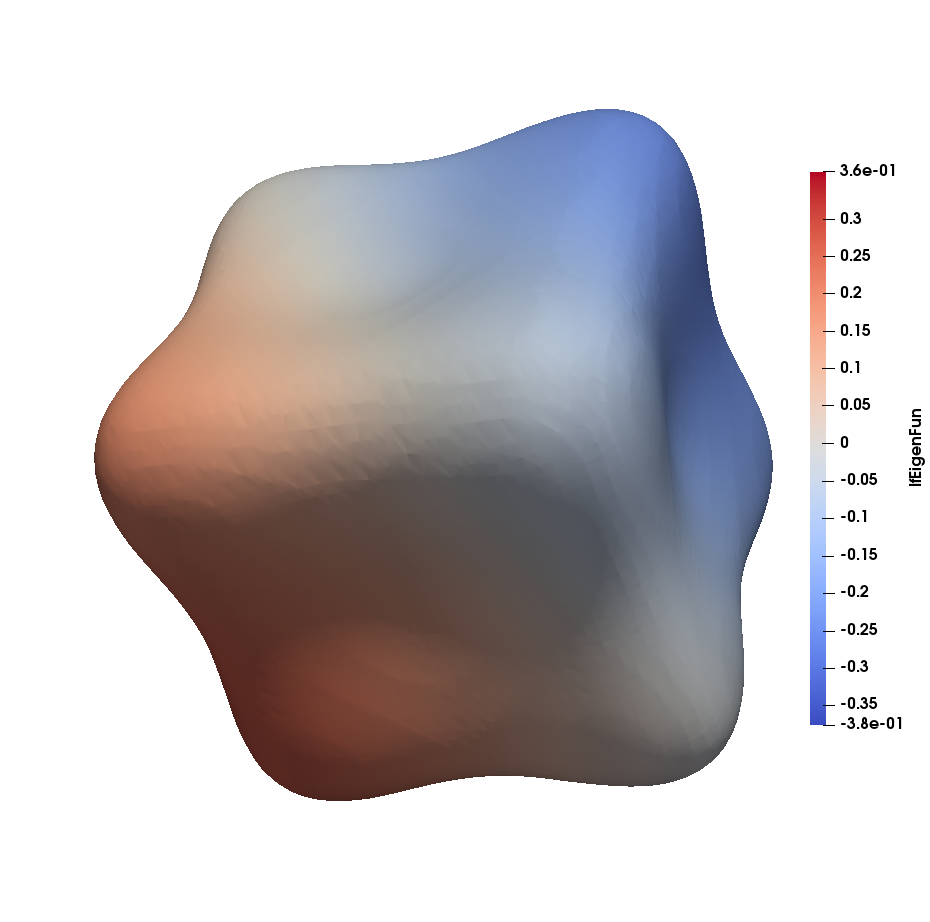
(b) $\lambda_{h,2}=0.5915189071$

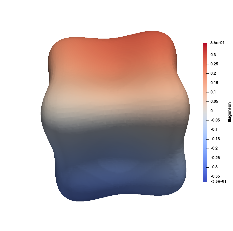
(c) $\lambda_{h,3}=0.5915189381$

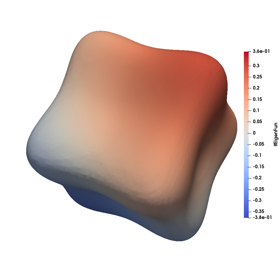
(d) $\lambda_{h,4}=0.5915934027$

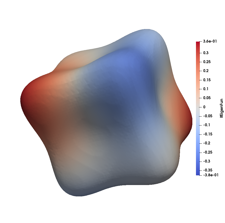
(e) $\lambda_{h,5}=1.612570362$

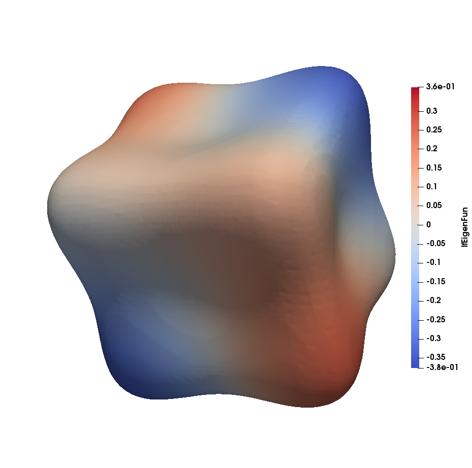
(f) $\lambda_{h,6}=1.612570431$

Figure 6: The Laplace-Beltrami eigenvalues and eigenfunctions on a general surface.

7 Conclusion

In this paper, we develop a new trace finite element method for partial differential equations on the smooth surfaces. There is no geometric error in the discretization of the surface since numerical integration is done directly on the surfaces. We focus on the Laplace-Beltrami eigenvalue problems, which have not been studied by the trace finite element methods. The difficulties arise from the fact that the dimension of the finite element space is usually smaller than the degree of freedoms. Therefore, the direct application of the trace FEM to the eigenvalue problem will lead to many false eigenvalues.

We analyse carefully the eigenvalues of the discrete problems of the trace FEM and show that the geometric consistency property of the trace FEMs can improve the situation largely. Theoretically, it is possible that the discrete system of our method does not have any false eigenvalues if the surface is not a part of the zero level-set of some finite element function defined in the bulk domain. This is also verified by our numerical experiments. Furthermore, for the corresponding generalized matrix eigenvalue problem with false eigenvalues, we show that a perturbed method can be used to compute the true eigenvalues. It turns out that the algorithm works well for both the standard trace finite element method and the geometric consistent method. Our experiments also show that the geometric consistent method improves the accuracy dramatically in comparison with the traditional methods. We present a numerical analysis of our method for both the Laplace-Beltrami equation and the corresponding eigenvalue problem. In comparison to the methods defined on the discrete surface, the analysis becomes much simpler. Our method can also be easily extended to any higher order finite element methods by considering proper higher order numerical quadrature on the smooth surface.

In this work, we mainly focus on the approximation property of the method. It is known that the condition number of the trace finite element method might be large due to the irregular surface mesh induced by the bulk triangulations [58, 61]. Usually some stabilization terms can be added to the method to improve the numerical stability [9, 11, 42, 44]. These techniques can be used in our method as well and it might become necessary for higher order methods. This will be left for future work.

References

- [1] M. Arroyo and A. DeSimone, Relaxation dynamics of fluid membranes, Physical review E, 79 (2009), p. 031915.
- [2] I. Babuška and J. Osborn, Eigenvalue problems, (1991).
- [3] E. Bachini, M. W. Farthing, and M. Putti, Intrinsic finite element method for advection-diffusion-reaction equations on surfaces, Journal of Computational Physics, 424 (2021), p. 109827.
- [4] J. T. Beale, Solving partial differential equations on closed surfaces with planar cartesian grids, SIAM Journal on Scientific Computing, 42 (2020), pp. A1052–A1070.
- [5] M. Bertalmio, L.-T. Cheng, S. Osher, and S. Guillermo, Variational problems and partial differential equations on implicit surfaces: The framework and examples in image processing and pattern formation, (2000).
- [6] M. Bertalmio, G. Sapiro, L.-T. Cheng, and S. Osher, A framework for solving surface partial differential equations for computer graphics applications, CAM Report 00-43, UCLA, Mathematics Department, 3 (2000).
- [7] D. Boffi, Finite element approximation of eigenvalue problems, Acta Numerica, 19 (2010), pp. 1–120.
- [8] A. Bonito, A. Demlow, and R. H. Nochetto, Finite element methods for the laplace–beltrami operator, arXiv: Numerical Analysis, 21 (2020), pp. 1–103.
- [9] E. Burman, P. Hansbo, and M. G. Larson, A stabilized cut finite element method for partial differential equations on surfaces: the laplace–beltrami operator, Computer Methods in Applied Mechanics and Engineering, 285 (2015), pp. 188–207.
- [10] E. Burman, P. Hansbo, M. G. Larson, and A. Massing, A cut discontinuous Galerkin method for the Laplace–Beltrami operator, IMA Journal of Numerical Analysis, 37 (2017), pp. 138–169.
- [11] E. Burman, P. Hansbo, M. G. Larson, A. Massing, and S. Zahedi, Full gradient stabilized cut finite element methods for surface partial differential equations, Computer Methods in Applied Mechanics and Engineering, 310 (2016), pp. 278–296.
- [12] P. Buser, Geometry and spectra of compact Riemann surfaces, Springer Science & Business Media, 2010.
- [13] A. Y. Chernyshenko and M. A. Olshanskii, An adaptive octree finite element method for PDEs posed on surfaces, Computer Methods in Applied Mechanics and Engineering, 291 (2015), pp. 146–172.
- [14] P. G. Ciarlet, The finite element method for elliptic problems, SIAM, 2002.
- [15] M.-E. Craioveanu, M. Puta, and T. RASSIAS, Old and new aspects in spectral geometry, vol. 534, Springer Science & Business Media, 2013.
- [16] T. Cui, W. Leng, H. Liu, L. Zhang, and W. Zheng, High-order numerical quadratures in a tetrahedron with an implicitly defined curved interface, ACM Transactions on Mathematical Software, 46 (2020), pp. 1–18.
- [17] K. Deckelnick, G. Dziuk, C. M. Elliott, and C.-J. Heine, An h-narrow band finite-element method for elliptic equations on implicit surfaces, IMA Journal of Numerical Analysis, 30 (2010), pp. 351–376.
- [18] L. Dedè and A. Quarteroni, Isogeometric analysis for second order partial differential equations on surfaces, Computer Methods in Applied Mechanics and Engineering, 284 (2015), pp. 807–834.
- [19] A. Demlow, Higher-order finite element methods and pointwise error estimates for elliptic problems on surfaces, SIAM Journal on Numerical Analysis, 47 (2009), pp. 805–827.
- [20] A. Demlow and G. Dziuk, An adaptive finite element method for the laplace–beltrami operator on implicitly defined surfaces, SIAM Journal on Numerical Analysis, 45 (2007), pp. 421–442.
- [21] J. Demmel, Generalized non-hermitian eigenproblems, in Templates for the solution of algebraic eigenvalue problems: a practical guide, edit by Bai, Zhaojun and Demmel, James and Dongarra, Jack and Ruhe, Axel and van der Vorst, Henk, pp. 28–36.
- [22] J. Demmel and B. Kågström, The generalized schur decomposition of an arbitrary pencil a–b—robust software with error bounds and applications. part i: theory and algorithms, ACM Transactions on Mathematical Software (TOMS), 19 (1993), pp. 160–174.
- [23] G. Dong, H. Guo, and Z. Shi, Discontinuous galerkin methods for the laplace-beltrami operator on point cloud, arXiv preprint arXiv:2012.15433, (2020).
-
[24]
DROPS package.
http://www.igpm.rwth-aachen.de/DROPS/. - [25] Q. Du, M. D. Gunzburger, and L. Ju, Voronoi-based finite volume methods, optimal voronoi meshes, and pdes on the sphere, Computer methods in applied mechanics and engineering, 192 (2003), pp. 3933–3957.
- [26] G. Dziuk, Finite elements for the beltrami operator on arbitrary surfaces, (1988).
- [27] G. Dziuk and C. M. Elliott, Finite elements on evolving surfaces, IMA journal of numerical analysis, 27 (2007), pp. 262–292.
- [28] , Surface finite elements for parabolic equations, Journal of Computational Mathematics, (2007), pp. 385–407.
- [29] , Finite element methods for surface pdes, Acta Numerica, 22 (2013), p. 289.
- [30] C. M. Elliott and B. Stinner, Modeling and computation of two phase geometric biomembranes using surface finite elements, Journal of Computational Physics, 226 (2007), pp. 1271–1290.
- [31] M. H. Gfrerer and M. Schanz, A high-order fem with exact geometry description for the laplacian on implicitly defined surfaces, International Journal for Numerical Methods in Engineering, 114 (2018), pp. 1163–1178.
- [32] R. Glowinski and D. C. Sorensen, Computing the eigenvalues of the laplace-beltrami operator on the surface of a torus: A numerical approach, in Partial differential equations, Springer, 2008, pp. 225–232.
- [33] C. Gordon, D. Webb, and S. Wolpert, Isospectral plane domains and surfaces via riemannian orbifolds, Inventiones mathematicae, 110 (1992), pp. 1–22.
- [34] C. Gordon, D. L. Webb, and S. Wolpert, One cannot hear the shape of a drum, Bulletin of the American Mathematical Society, 27 (1992), pp. 134–138.
- [35] J. Grande, Eulerian finite element methods for parabolic equations on moving surfaces, SIAM journal on scientific computing, 36 (2014), pp. B248–B271.
- [36] J. Grande, C. Lehrenfeld, and A. Reusken, Analysis of a high-order trace finite element method for pdes on level set surfaces, SIAM Journal on Numerical Analysis, 56 (2018), pp. 228–255.
- [37] J. Grande and A. Reusken, A higher order finite element method for partial differential equations on surfaces, SIAM Journal on Numerical Analysis, 54 (2016), pp. 388–414.
- [38] S. Groß and A. Reusken, Numerical Methods for Two-phase Incompressible Flows, Springer, Berlin, 2011.
- [39] E. Hebey, Sobolev spaces on Riemannian manifolds, vol. 1635, Springer Science & Business Media, 1996.
- [40] M. E. Hochstenbach, C. Mehl, and B. Plestenjak, Solving singular generalized eigenvalue problems by a rank-completing perturbation, SIAM Journal on Matrix Analysis and Applications, 40 (2019), pp. 1022–1046.
- [41] B. Kovács, High-order evolving surface finite element method for parabolic problems on evolving surfaces, IMA Journal of Numerical Analysis, 38 (2018), pp. 430–459.
- [42] M. G. Larson and S. Zahedi, Stabilization of high order cut finite element methods on surfaces, IMA Journal of Numerical Analysis, 40 (2020), pp. 1702–1745.
- [43] C. Lehrenfeld, High order unfitted finite element methods on level set domains using isoparametric mappings, Computer Methods in Applied Mechanics and Engineering, 300 (2016), pp. 716–733.
- [44] C. Lehrenfeld, M. A. Olshanskii, and X. Xu, A stabilized trace finite element method for partial differential equations on evolving surfaces, SIAM Journal on Numerical Analysis, 56 (2018), pp. 1643–1672.
- [45] E. Lehto, V. Shankar, and G. B. Wright, A radial basis function (rbf) compact finite difference (fd) scheme for reaction-diffusion equations on surfaces, SIAM Journal on Scientific Computing, 39 (2017), pp. A2129–A2151.
- [46] S. Leung, J. Lowengrub, and H. Zhao, A grid based particle method for solving partial differential equations on evolving surfaces and modeling high order geometrical motion, Journal of Computational Physics, 230 (2011), pp. 2540–2561.
- [47] Z. Li and Z. Shi, A convergent point integral method for isotropic elliptic equations on a point cloud, Multiscale Modeling & Simulation, 14 (2016), pp. 874–905.
- [48] J. Liang and H. Zhao, Solving partial differential equations on point clouds, SIAM Journal on Scientific Computing, 35 (2013), pp. A1461–A1486.
- [49] C. B. Macdonald, J. Brandman, and S. J. Ruuth, Solving eigenvalue problems on curved surfaces using the closest point method, Journal of Computational Physics, 230 (2011), pp. 7944–7956.
- [50] H. P. McKean Jr and I. M. Singer, Curvature and the eigenvalues of the laplacian, Journal of Differential Geometry, 1 (1967), pp. 43–69.
- [51] W. Milliken, H. Stone, and L. Leal, The effect of surfactant on transient motion of newtonian drops, Phys. Fluids A, 5 (1993), pp. 69–79.
- [52] A. Muhič and B. Plestenjak, On the singular two-parameter eigenvalue problem, The Electronic Journal of Linear Algebra, 18 (2009), pp. 420–437.
- [53] B. Müller, F. Kummer, and M. Oberlack, Highly accurate surface and volume integration on implicit domains by means of moment-fitting, International Journal for Numerical Methods in Engineering, 96 (2013), pp. 512–528.
- [54] A. Nasikun, C. Brandt, and K. Hildebrandt, Fast approximation of laplace-beltrami eigenproblems, in Computer Graphics Forum, vol. 37, Wiley Online Library, 2018, pp. 121–134.
- [55] I. L. Novak, F. Gao, Y.-S. Choi, D. Resasco, J. C. Schaff, and B. Slepchenko, Diffusion on a curved surface coupled to diffusion in the volume: application to cell biology, Journal of Computational Physics, 229 (2010), pp. 6585–6612.
- [56] M. Olshanskii, A. Reusken, and A. Zhiliakov, Inf-sup stability of the trace p2-p1 taylor–hood elements for surface pdes, Mathematics of Computation, 90 (2021), pp. 1527–1555.
- [57] M. Olshanskii, X. Xu, and V. Yushutin, A finite element method for allen–cahn equation on deforming surface, Computers & Mathematics with Applications, 90 (2021), pp. 148–158.
- [58] M. A. Olshanskii and A. Reusken, A finite element method for surface pdes: matrix properties, Numerische Mathematik, 114 (2010), p. 491.
- [59] , Trace finite element methods for pdes on surfaces, in Geometrically unfitted finite element methods and applications, Springer, 2017, pp. 211–258.
- [60] M. A. Olshanskii, A. Reusken, and J. Grande, A finite element method for elliptic equations on surfaces, SIAM Journal on Numerical Analysis, 47 (2009), pp. 3339–3358.
- [61] M. A. Olshanskii, A. Reusken, and X. Xu, On surface meshes induced by level set functions, Computing and visualization in science, 15 (2012), pp. 53–60.
- [62] , An Eulerian space–time finite element method for diffusion problems on evolving surfaces, SIAM Journal on Numerical Analysis, 52 (2014), pp. 1354–1377.
-
[63]
PHG package.
http://lsec.cc.ac.cn/phg/. - [64] A. Reusken, Analysis of trace finite element methods for surface partial differential equations, IMA Journal of Numerical Analysis, 35 (2015), pp. 1568–1590.
- [65] M. Reuter, F.-E. Wolter, and N. Peinecke, Laplace–beltrami spectra as ‘shape-dna’of surfaces and solids, Computer-Aided Design, 38 (2006), pp. 342–366.
- [66] S. J. Ruuth and B. Merriman, A simple embedding method for solving partial differential equations on surfaces, Journal of Computational Physics, 227 (2008), pp. 1943–1961.
- [67] R. Saye, High-order quadrature methods for implicitly defined surfaces and volumes in hyperrectangles, SIAM Journal on Scientific Computing, 37 (2015), pp. A993–A1019.
- [68] K. Simons and E. Ikonen, Functional rafts in cell membranes, Nature, 387 (1997), p. 569.
- [69] H. Stone, A simple derivation of the time-dependent convective-diffusion equation for surfactant transport along a deforming interface, Phys. Fluids A, 2 (1990), pp. 111–112.
- [70] J. Sun and A. Zhou, Finite element methods for eigenvalue problems, Chapman and Hall/CRC, 2016.
- [71] P. Van Dooren, The computation of kronecker’s canonical form of a singular pencil, Linear Algebra and Its Applications, 27 (1979), pp. 103–140.
- [72] H. Weyl, Das asymptotische verteilungsgesetz der eigenwerte linearer partieller differentialgleichungen (mit einer anwendung auf die theorie der hohlraumstrahlung), Mathematische Annalen, 71 (1912), pp. 441–479.
- [73] J. H. Wilkinson, Kronecker’s canonical form and the qz algorithm, Linear Algebra and its Applications, 28 (1979), pp. 285–303.
- [74] G. Xu, Discrete laplace–beltrami operators and their convergence, Computer aided geometric design, 21 (2004), pp. 767–784.
- [75] J.-J. Xu and H.-K. Zhao, An Eulerian formulation for solving partial differential equations along a moving interface, Journal of Scientific Computing, 19 (2003), pp. 573–594.
- [76] V. Yushutin, A. Quaini, and M. Olshanskii, Numerical modeling of phase separation on dynamic surfaces, Journal of Computational Physics, 407 (2020), p. 109126.