Deep Neural Networks and PIDE discretizations

Abstract

In this paper, we propose neural networks that tackle the problems of stability and field-of-view of a Convolutional Neural Network (CNN). As an alternative to increasing the network’s depth or width to improve performance, we propose integral-based spatially nonlocal operators which are related to global weighted Laplacian, fractional Laplacian and inverse fractional Laplacian operators that arise in several problems in the physical sciences. The forward propagation of such networks is inspired by partial integro-differential equations (PIDEs). We test the effectiveness of the proposed neural architectures on benchmark image classification datasets and semantic segmentation tasks in autonomous driving. Moreover, we investigate the extra computational costs of these dense operators and the stability of forward propagation of the proposed neural networks.

65D15, 65L07, 68T05, 68W25, 47G20, 47G30

1 Introduction

We consider the tasks of image classification and segmentation which can be seen as a data fitting problem in a high-dimensional space. Image classification involves assigning each element of a dataset to one of the many classes or categories of images. It forms the basis for several other computer vision tasks such as detection, segmentation and localization. Let each $C$-channel image be of dimension $\mathbb{R}^{H\times W\times C}$, with each image belonging to one of the $k$ classes. Then the objective is to find a classifier map $\mathcal{J}:\mathbb{R}^{H\times W\times C}\mapsto\mathbb{R}^{k}$ such that, for a given $\mathbf{x}\in\mathbb{R}^{H\times W\times C}$, we have $\mathcal{J}(\mathbf{x})\approx p(\mathbf{x})\in\mathbb{R}^{k}$, where $p(\mathbf{x})$ represents the probabilities of $\mathbf{x}$ belonging to one of the $k$ classes. The task of semantic segmentation is similar and can be seen as a multi-dimensional extension of the image classification task. Here, each pixel of each image is supposed to be assigned to one of the many classes (car, bus, etc.), i.e. each pixel gets a meaning so that, in the end, individual objects on an image can be distinguished from one another (see Section 5.3).

Deep Neural Networks (DNNs) can be used to train machines to learn from such examples, to recognize patterns in the data effectively and to make predictions on unseen examples [12]. DNNs have found several applications in the last decade, such as natural language processing [6] and solving partial differential equations (PDEs) [31], just to name a few. Convolutional Neural Networks (CNNs) are a special class of neural networks that make use of spatial correlations between features by introducing a series of spatial convolution operators into the network with compactly supported stencils/kernels and point-wise nonlinearities, where the trainable kernel weights capture hierarchical patterns. CNNs increase the computational efficiency of the network due to the sparse connections between the features and due to the reduction in the number of weights via parameter sharing. Moreover, in [42], it is argued that CNNs can approximate any continuous function to an arbitrary accuracy if the depth of the neural network is large enough.

There are several hurdles when it comes to designing and training a neural network. Firstly, there is the well-known issue of exploding and vanishing gradients [24]. Also, in CNNs, the convolution operation is local, and, as a consequence, each layer draws inferences based on the information that is present in a small spatial neighborhood of the image (receptive field) and therefore lacks a holistic view of the feature maps. This is known as the field-of-view problem [23]. To make sure that the output layer has a large receptive field and no information of the image is left out while making the inference, modern architectures tend to go deep [16, 30]. By stacking more convolutional and pooling layers, the receptive field is increased, and large parts of the image end up having an indirect influence on the output layer. This is helpful for datasets with long-range spatial dependencies. However, the number of trainable weights increases rapidly with depth, and this imposes challenges when using mediocre computational hardware with memory constraints. Thus, the dilemma is whether one should have a very deep network that has a better performance but makes the training harder for any optimizer or to have shallower networks that are easier to train but perform relatively worse.

To this end, we propose neural networks that tackle the field-of-view problem of a CNN. Instead of increasing the network’s depth or width to improve a neural network’s performance, the introduction of nonlocal operators is advocated. These integral-based spatially nonlocal operators address the issue of field-of-view and reduce the need for deeper networks if one needs better performance. The associated forward propagation is inspired by partial integro-differential equations (PIDEs). Specifically, a corresponding layer that is inspired by a specific PIDE system is added to a ResNet network of consecutive Hamiltonian blocks. We examine the effectiveness of the proposed network designs for several image classification benchmark datasets. Our networks need lesser depth than the conventional CNNs to obtain the same accuracy and expressibility while maintaining the numerical stability of the network. Additionally, this paper demonstrates a real-world application, namely our networks are used for semantic segmentation tasks in autonomous driving.

This paper is organized as follows. In Section 2, a general introduction to Residual Neural Networks (ResNets), its mathematical formulation and its link with stable dynamical systems is reviewed. Section 3 introduces the PIDE-inspired nonlocal operators, and a few inherent properties of such operators are explored and reviewed. These nonlocal operators are then discretized in Section 4, and several strategies to save computational costs are proposed. In this section, also the implementation details for the nonlocal operators and the proposed CNNs are discussed. In Section 5, numerical experiments related to image classification and semantic segmentation are conducted, and their effectiveness is examined. Section 6 deals with the forward propagation stability of the proposed CNNs and the computational cost associated with them. The concluding Section 7 summarizes the results.

2 Mathematical formulation

In this section, we briefly formulate the classification task as a parameter estimation problem. We also introduce the building blocks of the basic neural architecture that will be used in the subsequent sections of this paper. For a detailed summary of deep learning, see [12, 38].

Let $\mathbf{Y}_{0}$ be the input to the neural network. The forward propagation of a Residual Neural Network (ResNet) with $N$ layers is given by

(1) $$\mathbf{Y}_{j+1}=\mathbf{Y}_{j}+\mathcal{F}(\mathbf{Y}_{j},\mathbf{K}_{j})\quad\text{for }\>j=0,\ldots,N-1,$$

where $\mathbf{Y}_{j}$ are the feature values in the $j$-th hidden layer, $\mathbf{K}_{j}$ are the learnable (convolutional and batch normalization) weights in the $j$-th hidden layer, and $\mathcal{F}$ is the residual module that can come in various forms, for example, $\mathcal{F}(\mathbf{Y}_{j},\mathbf{K}_{j})=\sigma(\mathcal{B}(\mathbf{K}_{j,2}\,\sigma(\mathcal{B}(\mathbf{K}_{j,1}\mathbf{Y}_{j}+b_{j}))))$ [16], where $\mathbf{K}_{j}=\{\mathbf{K}_{j,1},\mathbf{K}_{j,2}\}$, i.e. the residual module has two convolutional layers. $\mathcal{B}$ represents the batch normalization (BN) layer [18] and $\sigma(\cdot)$ is the activation function applied component-wise. For our purposes, we will stick with the the rectifier or ReLU activation function, $\sigma(x)=\max(0,x)$. $\mathbf{Y}_{N}$ is the final layer of the neural network. For multi-class classification tasks, this final layer is passed through a softmax classifier, $S:\mathbb{R}^{k}\mapsto\mathbb{R}^{k}$, $[S(x)]_{i}:=\frac{e^{x_{i}}}{\sum_{j=1}^{k}e^{x_{j}}}$. It returns the necessary probability distribution consisting of $k$ probabilities that are proportional to the entries of the input vector $x$ and are actually the different probabilities of the image/pixel belonging to each of the $k$ classes.

Essentially, in each step of the iteration, the residual module tries to learn the update made to $\mathbf{Y}_{j}$. Note that the residual module depends not just on layer weights $\mathbf{K}_{j}$, but also on layer biases $b_{j}$. For simplicity, however, we write $\mathcal{F}(\mathbf{Y}_{j},\mathbf{K}_{j})$ instead of $\mathcal{F}(\mathbf{Y}_{j},\mathbf{K}_{j},b_{j})$. In the original paper [16], this residual block followed the sequence of convolution-BN-ReLU. In a follow-up paper [17], He, Zhang, Ren et al. suggest another sequence for computations, namely BN-ReLU-convolution. Over the last couple of years, ResNet has had a lot of success in several areas, such as object detection [15, 16] and semantic segmentation [25]. ResNets have made it possible to train up to hundreds of layers and still achieve compelling performance, something which was not possible before. Szegedy, Ioffe, Vanhoucke et al. showed in [36] that residual links in fact speed up the convergence of very deep networks.

Let the output of the softmax layer be called $\mathbf{Y}_{N+1}$, with $\mathbf{W}$ representing the weights and biases of this extra layer. Let the collection of weights and biases of the other layers be represented as $\mathbf{K}=\{\mathbf{K}_{j}\}_{j=1}^{j=N}$, $b=\{b_{j}\}_{j=1}^{j=N}$, respectively. Then the learning problem can be cast as a high-dimensional, non-convex optimization problem

(2) $$\begin{aligned} &\min_{\mathbf{K},\mathbf{W},b}&&\frac{1}{2}S(\mathbf{Y}_{N+1},\mathbf{C})+R(\mathbf{K},\mathbf{W},b)\\ \text{such }&\text{that}&&\mathbf{Y}_{j+1}=\mathbf{Y}_{j}+\mathcal{F}(\mathbf{Y}_{j},\mathbf{K}_{j})\quad\text{for }\>j=0,\ldots,N-1,\\ \end{aligned}$$

where $S$ is the loss function that is convex in the first argument and measures the closeness of the prediction to the ground truth. Usually, $S$ is assumed to be the least-squares function and cross-entropy loss function for regression and classification tasks, respectively [12]. $\mathbf{C}$ is the label or the ground truth for the example $\mathbf{Y}_{0}$ that is propagated through the network. $R$ is a convex regularizer that penalizes large weights that are undesirable (see Section 4.5).

The forward propagation of a ResNet can be interpreted as a discretization of an underlying nonlinear ordinary differential equation (ODE), and in special cases, as a discretization of an underlying partial differential equation (PDE). We add a step size $h$ to the equation of the forward propagation of ResNets [10, 14], i.e.

(3) $$\mathbf{Y}_{j+1}=\mathbf{Y}_{j}+h\mathcal{F}(\mathbf{Y}_{j},\mathbf{K}_{j})\quad\text{for }\>j=0,\ldots,N-1.$$

This equation can be interpreted as a forward Euler discretization of the initial value problem

(4) $$\dot{\mathbf{Y}}(t)=\mathcal{F}(\mathbf{Y}(t),\mathbf{K}(t)),\quad\mathbf{Y}(0)=\mathbf{Y}_{0},$$

with the input layer being $\mathbf{Y}(0)$ and the output layer values $\mathbf{Y}(T)$ being the solution to the initial value problem at time $T$, with $T=Nh$, $T$ and $N$ being related to the depth of the network. Thus, each layer of the network can be seen as the discretization of the continuous solution at discrete time points in $[0,T]$, and the problem of learning the network weights $\mathbf{K}_{j}$ can be seen as a parameter estimation problem or an optimal control problem that is governed by equation (4). Moreover, in [41], Zhang, Han, Wynter et al. claim that the presence of the step size $h$ in ResNet-like networks stabilizes the gradients and allows larger learning rates.

With the introduction of the dummy time variable $t$, we have a time derivative in the forward propagation. In special cases, such as image classification or segmentation, one mainly has spatial convolution weights $\mathbf{K}_{j}$ for each layer, instead of dense weight matrices. In such cases, the convolution weights can be expressed as a linear combination of spatial differential operators or as a coupled system of partial differential operators in case of multi-channel convolutions [28]. As a result, in the case of CNNs, equation (1) is a forward Euler discretization (in the time domain) of an underlying partial differential equation due to the inherent presence of spatial derivatives in the residual function $\mathcal{F}$. The CNN layer weights determine the order, type and stability of the underlying PDE.

The stability of the forward propagation of a neural network is of prime importance. The output of a neural network or the solution to the underlying PDE/ODE is sensitive to perturbations of the input data that are not perceived by the human eye, which makes a network vulnerable to adversarial attacks [43]. Similar images might propagate through the network and yield vastly different outputs and predictions [13], and therefore the network generalizes poorly on test data. Also, such instabilities make the network harder to train via backpropagation. Chang, Meng, Haber et al. suggest several stable neural architectures in [4], which are inspired by stable and well-posed solutions of the underlying PDE/ODE of the neural network [4, 14]. Among all the three ODE-based networks suggested in [4], the so-called Hamiltonian network performs the best on standard benchmarks, possibly due to its two-layer network, where each Hamiltonian block has two convolution and two transposed convolution operations. Hamiltonian systems are known to conserve energy, and hence, the forward propagation, in this case, is expected to only moderately amplify or damp the features, as it is propagated down the network. By introducing an extra augmented variable $\mathbf{Z}(t)$ and two sets of convolution filters $\mathbf{K}_{1}(t),\mathbf{K}_{2}(t)$, the forward propagation can be interpreted as a Hamiltonian system, where we have a system of PDEs

(5) $$\begin{aligned} \dot{\mathbf{Y}}(t)&=\mathbf{K}_{1}^{T}(t)\,\sigma(\mathbf{K}_{1}(t)\mathbf{Z}(t)+b_{1}(t)),\\ \dot{\mathbf{Z}}(t)&=-\mathbf{K}_{2}^{T}(t)\,\sigma(\mathbf{K}_{2}(t)\mathbf{Y}(t)+b_{2}(t)).\end{aligned}$$

Here, $\mathbf{Y}(t)$ and $\mathbf{Z}(t)$ are channel-wise partitions of the input features, and for our purposes of image classification and segmentation, $\mathbf{K}_{i}(t)$ is the convolution operator, and $\mathbf{K}_{i}^{T}(t)$ is its transpose, $i=1,2$. The discretization of equation (5) is done using the Verlet integration since such symplectic methods capture the long time features of Hamiltonian systems really well [1]. With the Verlet scheme, we arrive at the following pair of coupled equations shown below. This computation is placed in a Hamiltonian block (see [4]).

(6) $$\begin{aligned} \mathbf{Y}_{j+1}&=\mathbf{Y}_{j}+h\,\mathbf{K}_{j1}^{T}\,\sigma(\mathbf{K}_{j1}\mathbf{Z}_{j}+b_{j1}),\\ \mathbf{Z}_{j+1}&=\mathbf{Z}_{j}-h\,\mathbf{K}_{j2}^{T}\,\sigma(\mathbf{K}_{j2}\mathbf{Y}_{j+1}+b_{j2}).\end{aligned}$$

3 Nonlocal and pseudo-differential operators for Deep Learning

In a Convolutional Neural Network, the pooling or subsampling of the image and the convolution operations allow far-away pixels in an image to communicate with each other, thereby exploiting long-range correlations in an image and improving the predictions made by the network. At the same time, convolution is a local operation, and therefore each convolutional layer’s values depend only on the information present in certain local patches of the image. This is known as the field-of-view problem [23]. The value of a neuron in a convolutional layer only depends on a certain subset of the input. This region in the input is the receptive field for that neuron. In learning tasks with images, each neuron in the output layer should ideally have a big receptive field, i.e. the values of the output neurons should indirectly depend on large parts of the image so that no important information of the image is left out when making the predictions. The receptive field size of a neuron can be increased, for example, by stacking more convolutional layers and thereby making the network deeper. This enlarges the receptive field size linearly in theory. Meanwhile, pooling or subsampling allows each pixel to cover a larger area and facilitates information travel over larger distances, which increases the receptive field size multiplicatively. However, just stacking up convolutional and pooling layers can have several disadvantages. In a deeper network, for example, the optimization problem (2) might be hard to solve and repeatedly performing local operations can be computationally inefficient.

In this article, we propose to employ additional layers which involve nonlocal interactions. Long-range and nonlocal dependencies are ubiquitous in several fields, such as financial markets [7], physical sciences [9], image denoising [2] or image regularization [11]. We thus look at a few integral-based spatially nonlocal operators that could be used in CNNs. The underlying and associated partial integro-differential equation (PIDE) is then discretized in a so-called nonlocal block and inserted in the neural network. By direct computation of interactions between each pair of pixels or pair of patches in an image, these operators make sure that the field-of-view increases drastically. Consequently, the information travels larger distances for a fixed number of layers in a neural network.

3.1 The nonlocal diffusion operator

Definition 3.1.

Let $\Omega\subseteq\mathbb{R}^{n}$ and let $v:\mathbb{R}^{n}\rightarrow\mathbb{R}^{n}$ be any function, then for $\mathbf{x},\mathbf{y}\in\Omega$, the nonlocal diffusion operator can be defined as

(7) $$\mathcal{L}v(\mathbf{x}):=\int\limits_{\Omega}\omega(\mathbf{x},\mathbf{y})[v(\mathbf{y})-v(\mathbf{x})]\,d\mathbf{y},$$

where the kernel $\omega$ has the following two properties: (i) $\omega$ is symmetric: $\omega(\mathbf{x},\mathbf{y})=\omega(\mathbf{y},\mathbf{x}),\\ \forall\mathbf{x},\mathbf{y}\in\Omega$ and (ii) $\omega$ is positivity-preserving: $\omega(\mathbf{x},\mathbf{y})\geq 0,\forall\mathbf{x},\mathbf{y}\in\Omega$.

The kernel can be viewed as a function that measures the affinity or similarity between points in $\Omega$. The aim is to apply such a spatial-only operator on a discrete image $v$, where $v:\Omega\rightarrow\mathbb{R}^{C}$ is the discrete image with $C$ channels, and $v(\mathbf{x})$ is the set of pixel values of all the channels at a discrete spatial point $\mathbf{x}\in\Omega$ from the image domain $\Omega$ (the pixel strips in Figure 2).

Such operators have been an upshot of several image processing tasks. For example, for $\mathbf{x},\mathbf{y}\in\Omega$, consider the functional $J(u,t):=\frac{1}{4}\int\limits_{\Omega\times\Omega}\omega(\mathbf{x},\mathbf{y})[u(\mathbf{x},t)-u(\mathbf{y},t)]^{2}\,d\mathbf{x}\,d\mathbf{y}$ which sums up weighted variations of the function $u$, which is similar to total variational denoising in image processing. While minimizing the functional, the corresponding Euler-Lagrange descent flow is given by

(8) $$u_{t}(\mathbf{x},t)=-J^{\prime}(u)(\mathbf{x},t)=-\int\limits_{\Omega}\omega(\mathbf{x},\mathbf{y})[u(\mathbf{x},t)-u(\mathbf{y},t)]\,d\mathbf{y}=\mathcal{L}u(\mathbf{x},t).$$

Therefore, starting from an initial input image $u_{0}(\mathbf{x})$, the associated partial integro-differential equation (PIDE) can be written as

(9) $$u_{t}(\mathbf{x},t)=\mathcal{L}u(\mathbf{x},t),\quad u(\mathbf{x},0)=u_{0}(\mathbf{x}),$$

which is essentially a nonlocal weighted linear diffusion equation. The kernel function $\omega:\Omega\times\Omega\rightarrow\mathbb{R}$ is here assumed to be of Hilbert-Schmidt type [26], i.e. $\int\limits_{\Omega}\int\limits_{\Omega}|\omega(\mathbf{x},\mathbf{y})|^{2}\,d\mathbf{x}\,d\mathbf{y}<\infty$. There are several interpretations of the nonlocal diffusion operator that arise, e.g., from a continuous generalization of graph Laplacians or from a random walk Markov chain on $\Omega$.

The nonlocal diffusion operator $\mathcal{L}$ has many properties that are similar to a typical elliptic operator, such as $-\mathcal{L}$ being positive semi-definite. It can be shown that the system governed by equation (9) has energy decay [11], i.e.

$$\frac{d}{dt}\|u(\mathbf{x},t)\|_{L^{2}}^{2}=\frac{d}{dt}\int\limits_{\Omega}u(\mathbf{x},t)^{2}\,d\mathbf{x}\leq 0\quad\text{ for all }\mathbf{x}\in\Omega,\quad\frac{d}{dt}\operatorname{Var}[u(\mathbf{x},t)]\leq 0,$$

where $u(\mathbf{x},t)$ is the solution of equation (9). Since the operator $\mathcal{L}$ performs diffusion, the features tend to smooth out over time, and hence reduce the variance of the image/features. We will see later that, though the nonlocal interactions help in image classification, over-using it can damp the features leading to loss of information (see Section 5.2).

Next, we look at a few pseudo-differential operators that can also be represented as integral-based global operators whose implementations introduce nonlocality into the neural network. The aim is to define a spatial operator $\mathcal{O}$ such that the associated forward propagation for a given input image (or set of feature maps) $u_{0}(\mathbf{x})$ is governed by a PIDE that is similar to the form

(10) $$u_{t}(\mathbf{x},t)=\mathcal{O}u(\mathbf{x},t),\quad u(\mathbf{x},0)=u_{0}(\mathbf{x}).$$

For instance, for a propagation following (9), we have ${\mathcal{O}}={\mathcal{L}}$.

3.2 The fractional Laplacian operator

Fractional differential operators appear in several interesting problems in physical sciences [3] or in financial mathematics [29]. Let us first define a few related concepts before we define the operator itself.

Definition 3.2.

Let $\Omega\subseteq\mathbb{R}^{n}$, $0<s<1$. The fractional-order Sobolev space is defined as

$$H^{s}(\Omega):=\bigg{\{}v\in L^{2}(\Omega):\int\limits_{\Omega}\int\limits_{\Omega}\frac{[v(\mathbf{y})-v(\mathbf{x})]^{2}}{|\mathbf{x}-\mathbf{y}|^{n+2s}}\,d\mathbf{y}\,d\mathbf{x}<\infty\bigg{\}},$$

where the Gagliardo seminorm and the norm are defined as

$$|v|_{H^{s}(\Omega)}^{2}:=\int\limits_{\Omega}\int\limits_{\Omega}\frac{[v(\mathbf{y})-v(\mathbf{x})]^{2}}{|\mathbf{x}-\mathbf{y}|^{n+2s}}\,d\mathbf{y}\,d\mathbf{x},\quad\|v\|_{H^{s}(\Omega)}:=\Big{(}\|v\|_{L^{2}(\Omega)}^{2}+|v|_{H^{s}(\Omega)}^{2}\Big{)}^{1/2}.$$

Definition 3.3.

For $v\in\mathcal{S}(\mathbb{R}^{n})$, i.e. the Schwartz space of rapidly decreasing $C^{\infty}$ functions on $\mathbb{R}^{n}$, $0<s<1$, the fractional Laplacian operator $(-\Delta)^{s}$ is defined as the singular integral operator

(11) $$(-\Delta)^{s}v(\mathbf{x}):=c_{n,s}\,P.V.\displaystyle\int\limits_{\mathbb{R}^{n}}\frac{[v(\mathbf{x})-v(\mathbf{y})]}{|\mathbf{x}-\mathbf{y}|^{n+2s}}\,d\mathbf{y}=c_{n,s}\,\lim_{\epsilon\to 0^{+}}\displaystyle\int\limits_{\mathbb{R}^{n}\setminus B_{\epsilon}(\mathbf{x})}\frac{[v(\mathbf{x})-v(\mathbf{y})]}{|\mathbf{x}-\mathbf{y}|^{n+2s}}\,d\mathbf{y},$$

where P.V. stands for the Cauchy principal value (of the improper integral), $c_{n,s}$ is a constant depending on $n$, $s$ and is defined as $c_{n,s}=\frac{4^{s}\Gamma(n/2+s)}{\pi^{n/2}|\Gamma(-s)|}$.

Note that this operator can be seen as a special case of the nonlocal diffusion operator defined by equation (7), with kernel $\omega(\mathbf{x},\mathbf{y})=|\mathbf{x}-\mathbf{y}|^{-(n+2s)}$ and with the flipped term $v(\mathbf{x})-v(\mathbf{y})$ instead of $v(\mathbf{y})-v(\mathbf{x})$. The term is flipped because we want both operators to be elliptic, and the corresponding Poisson problem for the nonlocal diffusion operator is written as $-\mathcal{L}v(\mathbf{x})=0$, i.e. with an extra negative sign in front, whereas for the pseudo-differential operator, we have $(-\Delta)^{s}v(\mathbf{x})=0$.

Connection to pseudo-differential operators

The operator (11) can in fact be defined as a pseudo-differential operator (see Section SM1 in the supplementary material for further details), which shows the origins of the operator and also characterizes the operator in the Fourier space. Let the Fourier transform and the inverse Fourier transform of $v\in\mathcal{S}(\mathbb{R}^{n})$ be denoted by $\hat{v}(\xi):=\mathscr{F}v(\xi)$ and $v(\mathbf{x}):=\mathscr{F}^{-1}\hat{v}(\mathbf{x})$, respectively. It can be then shown that the fractional Laplacian is the pseudo-differential operator [8] with the Fourier symbol $(2\pi|\xi|)^{2s}$ and satisfies

(12) $$\mathscr{F}((-\Delta)^{s}v)(\xi)=(2\pi|\xi|)^{2s}\,\hat{v}(\xi)\quad\text{ for }0<s\leq 1.$$

For $s=1$, we get the classical Laplacian $(-\Delta)$ with the Fourier symbol $(2\pi|\xi|)^{2}$, i.e.

$$-\Delta v(\mathbf{x}) =-\Delta(\mathscr{F}^{-1}\hat{v}(\mathbf{x}))=-\Delta\Big{[}\int\limits_{\mathbb{R}^{n}}\hat{v}(\xi)e^{2\pi i\mathbf{x}\cdot\xi}\,d\xi\Big{]}$$

$$=\int\limits_{\mathbb{R}^{n}}(2\pi|\xi|)^{2}\,\hat{v}(\xi)e^{2\pi i\mathbf{x}\cdot\xi}\,d\xi=\mathscr{F}^{-1}\bigg{(}(2\pi|\xi|)^{2}\,\hat{v}(\xi)\bigg{)}.$$

For classical PDE operators, the corresponding Fourier symbol is generally a polynomial in $\xi$, but by using symbols that are not only a function of $\xi$ but also a function $\mathbf{x}$, we arrive at a large plethora of pseudo-differential operators. It can be shown that the classical Laplacian is a limit case of the fractional one [33], i.e. for a certain class of bounded functions $v$, $\mathbf{x}\in\mathbb{R}^{n}$, we have the point-wise limits $\lim_{s\to 0^{+}}(-\Delta)^{s}v(\mathbf{x})=v(\mathbf{x})$, $\lim_{s\to 1^{-}}(-\Delta)^{s}v(\mathbf{x})=-\Delta v(\mathbf{x})$. Note that there are several other equivalent definitions of the fractional Laplacian operator that are defined via heat semi-groups [35], or as an inverse of the Riesz potential, etc. (see [21]). For our purposes of image classification and segmentation, we will be using the singular integral operator from Definition 3.3 that defines the output of the operator point-wise.

3.3 The inverse fractional Laplacian operator

Now we define an analogous operator $(-\Delta)^{-s}$ for $s>0$, i.e. an inverse fractional Laplacian, which, as we will see, is also a nonlocal operator. Note that, similar to equation (12), we have

(13) $$\mathscr{F}((-\Delta)^{-s}v)(\xi)=(2\pi|\xi|)^{-2s}\,\hat{v}(\xi)\quad\text{ for }0<s<n/2.$$

One needs the restriction $0<s<n/2$ because if $s\geq n/2$, the Fourier symbol/multiplier $(2\pi|\xi|)^{-2s}$ fails to define a tempered distribution [29]. The symbol $(2\pi|\xi|)^{-2s}$ is decaying with respect to $s$, and, in the sense of distributions (see [32]), such symbols have the Fourier inverse $\mathscr{F}^{-1}(|\xi|^{-2s})=c_{n,-s}|\mathbf{x}|^{-(n-2s)}$. Using the inverse property for convolutions $f\ast g=\mathscr{F}^{-1}\{\mathscr{F}\{f\}\cdot\mathscr{F}\{g\}\}$ and equation (13), we get the following definition.

Definition 3.4.

For $v\in\mathcal{S}(\mathbb{R}^{n})$, $0<s<n/2$, the inverse fractional Laplacian operator $(-\Delta)^{-s}$ is defined as the integral operator

(14) $$(-\Delta)^{-s}v(\mathbf{x}):=\Big{(}c_{n,-s}|\mathbf{x}|^{-(n-2s)}\Big{)}\ast v(\mathbf{x})=c_{n,-s}\int\limits_{\mathbb{R}^{n}}\frac{v(\mathbf{y})}{|\mathbf{x}-\mathbf{y}|^{n-2s}}\,d\mathbf{y},$$

where $c_{n,-s}$ is the constant given by $c_{n,-s}=\frac{\Gamma(n/2-s)}{4^{s}\pi^{n/2}\Gamma(s)}$.

The right-hand side of the definition is called the Riesz potential. This singular integral is well-defined, provided $v$ decays sufficiently rapidly at infinity (see [32]), for instance, if $v\in L^{p}(\mathbb{R}^{n})$ with $1\leq p<\frac{n}{2s}$.

Recently, a fundamental solution for the case $s=n/2$ has been proposed [34], which can also be used in the neural network as a nonlocal operation. As pointed out in [32], the logarithmic kernel defined below can be seen as a vague limit of the Riesz potentials defined by (14).

Definition 3.5.

Let $v\in\mathcal{S}(\mathbb{R}^{n})$ with $\int\limits_{\mathbb{R}^{n}}v=0$, $\mathbf{x}\in\mathbb{R}^{n}$, and $s=n/2$. Then we have

(15) $$(-\Delta)^{-s}v(\mathbf{x}):=c_{n}\int\limits_{\mathbb{R}^{n}}\bigg{(}-2\log|\mathbf{x}-\mathbf{y}|-\gamma\bigg{)}v(\mathbf{y})\,d\mathbf{y},$$

where the Euler-Mascheroni constant $\gamma$ is given by $\gamma=-\int\limits_{0}^{\infty}e^{-r}\log r\,dr\approx 0.5772156649$, and the constant $c_{n}$ is given by $c_{n}=\frac{1}{(4\pi)^{n/2}\Gamma(n/2)}$.

As such, the Riesz potential kernel $\frac{1}{|\mathbf{x}-\mathbf{y}|^{n-2s}}$ may not always satisfy the square-integrability condition. Besides, in the case of the $\log$ kernel from equation (15), the kernel is no longer positivity-preserving. While implementing these nonlocal operators for images, methods used to bypass this issue and to avoid the blowing up of values are discussed in Sections 4.3 and 4.4. It is interesting to note that the kernels of the pseudo-differential operators are translation invariant and isotropic. Also, from Definition 3.4, it is clear that the operators from equations (14) and (15) can be seen as convolutions on a global scale (spatially), whereas the operators $\mathcal{L}$ and $(-\Delta)^{s}$ from equations (7) and (11), respectively, define a diffusion-like operator on a global scale (spatially).

4 Implementation details

In this section, we first look at the implementation of the Hamiltonian network that will be used as the base network. Then, several discretization details about the nonlocal blocks, which contain the proposed integral operators, will be introduced. We explore a few strategies to reduce the computational effort of such global operators and discuss how the respective tensors are dealt with when such operators are applied on images or feature maps. Finally, the general implementation details for the numerical experiments, including the regularization techniques, are discussed.

4.1 Hamiltonian networks with Verlet scheme

The Hamiltonian network will be used as the base architecture to ensure stability of the forward propagation, and changes are made to it by introducing nonlocality in the network. Similar to the ResNet architecture, several of the Hamiltonian blocks [4] are stacked up to form a Unit and several of these reversible Units together form the entire network. Figure 1 shows a 2-Unit Hamiltonian network as an example, where we see that the input is passed through an initial convolution layer and then through each Unit of the network.

Figure 1: The Hamiltonian Network with two Units having three Hamiltonian reversible Blocks each when used for image classification.

Similar to the original ResNet architecture [16], after each Unit (of $m$ Hamiltonian blocks), a pooling operation reduces the feature map size by half, and the number of channels is increased by using a $1\times 1$ convolution layer (with ReLU). After the final Unit, the features are subsampled and passed on to the fully-connected layer (for image classification tasks), where the predictions are made. The number of Units is kept fixed.

In our case, the networks will always contain three Units, each of which has $m$ Hamiltonian blocks. In terms of the ODE/PDE interpretation, each block represents a time step of the discretization, and the final output $\mathbf{Y}_{N}$ is the output of the last block in this network. Therefore, a normal Hamiltonian network has $12m+2$ layers, with $4m$ layers in each Unit (2 convolutions and 2 transposed convolutions per Hamiltonian block). To include the global operators into the network the nonlocality is added after the second Hamiltonian block in each Unit, i.e. the feature maps obtained after the second block are passed through the nonlocal block. The output of the nonlocal block is then fed into the next normal Hamiltonian block. Hence, altogether we have three additional nonlocal blocks in our network, one in each Unit.

4.2 Nonlocal diffusion operator

Let $\mathbf{X}\in\mathbb{R}^{H\times W\times C}$ be the input to the nonlocal block that is supposed to contain the nonlocal interactions. Let $\mathbf{X}_{i}$ denote each pixel of the image, i.e. for an input $\mathbf{X}$ with $C$ channels, $\mathbf{X}_{i}\in\mathbb{R}^{C}$ stands for the $C$ channel values for each pixel position. These vectors will be called pixel strips from here on. To implement the nonlocal diffusion operator $\mathcal{L}$ defined by equation (7) in the nonlocal block, we discretize the PIDE-inspired operator using a 2-step computation, which strengthens the nonlocal interactions between the features:

(16) $$\begin{aligned} \mathbf{[}\mathbf{B}_{1}]_{i}&=\mathbf{X}_{i}+h\,\mathcal{K}_{1}\Bigg{[}\displaystyle\frac{1}{\displaystyle\sum_{j}\omega(\mathbf{X}_{i},\mathbf{X}_{j})}\,{{\sum}}_{j}\omega(\mathbf{X}_{i},\mathbf{X}_{j})(\mathbf{X}_{j}-\mathbf{X}_{i})\Bigg{]},\\ [\mathbf{B}_{2}]_{i}&=\mathbf{X}_{i}+h\,\mathcal{K}_{2}\Bigg{[}\displaystyle\frac{1}{\displaystyle\sum_{j}\omega(\mathbf{X}_{i},\mathbf{X}_{j})}\,{{\sum}}_{j}\omega(\mathbf{X}_{i},\mathbf{X}_{j})\Big{(}[\mathbf{B}_{1}]_{j}-[\mathbf{B}_{1}]_{i}\Big{)}\Bigg{]},\end{aligned}$$

where $[\mathbf{B}_{1}]_{i}$ and $[\mathbf{B}_{2}]_{i}$ are the individual pixel strips of the intermediate feature maps $\mathbf{B}_{1}$ and the output feature maps $\mathbf{B}_{2}$ respectively, $h$ is the discretization step size, and $\mathcal{K}_{1}$, $\mathcal{K}_{2}$ are $1\times 1$ convolution operators, followed by ReLU activation and batch normalization. The output $\mathbf{B}_{2}$ is then fed into the next normal block in the Unit.

Relation to Verlet time-discretization

Let us investigate how (16) can be interpreted as a Verlet time-discretization of a system of ODEs, which represent a spatial discretization of the PIDE (10). To this end, set $\mathbf{V}^{\text{old}}:=\mathbf{X}^{\text{old}}:=\mathbf{X}\in\mathbb{R}^{C\times HW}$ and $\mathbf{W}^{\text{old}}:=-\mathbf{X}^{\text{old}}\in\mathbb{R}^{C\times HW}$. Now, for $i=1,\ldots,H\times W$, we define a two-step iteration scheme by

(17) $$\begin{aligned} \mathbf{V}_{i}^{\text{new}}&=\mathbf{V}_{i}^{\text{old}}+h\,\mathcal{K}_{1}\Bigg{[}\displaystyle\frac{1}{\displaystyle\sum_{j}\omega(\mathbf{V}_{i}^{\text{old}},\mathbf{V}_{j}^{\text{old}})}\,{{\sum}}_{j}\omega(\mathbf{V}_{i}^{\text{old}},\mathbf{V}_{j}^{\text{old}})(\mathbf{W}_{i}^{\text{old}}-\mathbf{W}_{j}^{\text{old}})\Bigg{]},\\ \mathbf{W}_{i}^{\text{new}}&=\mathbf{W}_{i}^{\text{old}}-h\,\mathcal{K}_{2}\Bigg{[}\displaystyle\frac{1}{\displaystyle\sum_{j}\omega(-\mathbf{W}_{i}^{\text{old}},-\mathbf{W}_{j}^{\text{old}})}\,{{\sum}}_{j}\omega(-\mathbf{W}_{i}^{\text{old}},-\mathbf{W}_{j}^{\text{old}})\Big{(}\mathbf{V}_{j}^{\text{new}}-\mathbf{V}_{i}^{\text{new}}\Big{)}\Bigg{]}.\end{aligned}$$

We directly see that $\mathbf{V}_{i}^{\text{new}}=[\mathbf{B}_{1}]_{i}$ and $\mathbf{X}^{\text{new}}_{i}:=-\mathbf{W}_{i}^{\text{new}}=[\mathbf{B}_{2}]_{i}$. Moreover, (17) is a Verlet scheme for a specific system of PIDEs as we will see now. To this end, let the $\mathbb{R}^{HW\times HW}$-valued operators $\Omega_{1},\Omega_{2}$ be defined by

$$\Big{[}\Omega_{1}(\mathbf{X})\Big{]}_{jk}:=\frac{\omega(\mathbf{X}_{j},\mathbf{X}_{k})}{\sum_{m}\omega(\mathbf{X}_{k},\mathbf{X}_{m})}~{}~{}~{}\text{ and }~{}~{}~{}\Big{[}\Omega_{2}(\mathbf{X})\Big{]}_{jk}:=\frac{\omega(-\mathbf{X}_{j},-\mathbf{X}_{k})}{\sum_{m}\omega(-\mathbf{X}_{k},-\mathbf{X}_{m})}.$$

Note that $\Omega_{1}(\mathbf{V}^{\text{old}})=\Omega_{2}(\mathbf{W}^{\text{old}})$. Furthermore, we define the operator $\operatorname{Diff}:\mathbb{R}^{C\times HW}\to\mathbb{R}^{HW\times HW\times C}$ by $\Big{[}\operatorname{Diff}(\mathbf{X})\Big{]}_{jk}=\mathbf{X}_{k}-\mathbf{X}_{j}$. With these operators we rewrite (17) as matrix/tensor equation

$$\begin{aligned} \mathbf{V}^{\text{new}}&=\mathbf{V}^{\text{old}}+h\,\mathcal{K}_{1}\Bigg{[}\operatorname{diag}_{12}\Big{(}\Omega_{1}(\mathbf{V}^{\text{old}})\operatorname{Diff}(\mathbf{W}^{\text{old}})\Big{)}^{T}\Bigg{]},\\ \mathbf{W}^{\text{new}}&=\mathbf{W}^{\text{old}}-h\,\mathcal{K}_{2}\Bigg{[}-\operatorname{diag}_{12}\Big{(}\Omega_{2}(\mathbf{W}^{\text{old}})\operatorname{Diff}(\mathbf{V}^{\text{new}})\Big{)}^{T}\Bigg{]},\end{aligned}$$

where $\operatorname{diag}_{12}:\mathbb{R}^{HW\times HW\times C}\to\mathbb{R}^{HW\times C}$ denotes the diagonal operator with respect to the first two dimensions, i.e. $[\operatorname{diag}_{12}(\mathbf{Y})]_{jk}:=\mathbf{Y}_{jjk}$. Note that the multiplication of $\Omega_{1}$ or $\Omega_{2}$ with the output of the $\operatorname{Diff}$ operator has to be understood in analogy to a multiplication between a $HW\times HW$ matrix and a $HW\times HWC$ matrix. With this, we can finally define the nonlinear system of ODEs

(18) $$\begin{aligned} \dot{\mathbf{V}}(t)&=\mathcal{K}_{1}(t)\Bigg{(}\operatorname{diag}_{12}\Big{(}\Omega_{1}(\mathbf{V}(t))\operatorname{Diff}(\mathbf{W}(t))\Big{)}^{T}\Bigg{)},\\ \dot{\mathbf{W}}(t)&=-\mathcal{K}_{2}(t)\Bigg{(}-\operatorname{diag}_{12}\Big{(}\Omega_{2}(\mathbf{W}(t))\operatorname{Diff}(\mathbf{V}(t))\Big{)}^{T}\Bigg{)}.\end{aligned}$$

Now it is easy to observe that the Verlet time-discretization of this system results in (17). The latter resembles a spatially discretized variant of

$$u_{t}(\mathbf{x},t)=\mathcal{O}u(\mathbf{x},t),\quad u(\mathbf{x},0)=u_{0}(\mathbf{x}),$$

with ${\mathcal{O}}={\mathcal{L}}$ and an additional outer convolution by $\mathcal{K}_{1}$ and $\mathcal{K}_{2}$. This has to be seen as an analogy to the system (5) and its time-discretization (6) from [4]. Thus, our nonlocal block iteration (16) resembles the Verlet discretization of a specific spatially discretized PIDE.

Affinity kernel and outer convolution

There are several things to note here regarding the kernel and the $1\times 1$ convolution. The kernel $\omega(\mathbf{x},\mathbf{y})$ measures the affinity or similarity between each pair of pixel strips of the image/feature maps. For choosing the right kernel, there are several suggestions made by Wang, Girshick, Gupta et al. in [39], such as the Gaussian function $e^{\mathbf{x}^{T}\mathbf{y}}$, the embedded Gaussian $e^{\theta(\mathbf{x})^{T}\phi(\mathbf{y})}$ and the embedded dot product $\theta(\mathbf{x})^{T}\phi(\mathbf{y})$. All these kernels seem to work equally well. We will be using the scaled embedded dot product $\lambda\theta(\mathbf{x})^{T}\phi(\mathbf{y})$, where $\theta$ and $\phi$ are $1\times 1$ convolutional embeddings, and $\lambda>0$ is a scaling factor. Essentially, it means that the input $\mathbf{X}$ is passed through two different $1\times 1$ convolutions to obtain embeddings $\theta(\mathbf{X})$ and $\phi(\mathbf{X})$. Then the kernel $\omega$ measures the affinity between the pairs of pixel strips $\theta(\mathbf{X}_{i})$ and $\phi(\mathbf{X}_{j})$ (see Figure 2). To reduce complexity, subsampling, e.g. pooling, can be applied within a pixel strip, see Figure 2 (right).

One can also use the scaled Gaussian kernel if one needs a positivity-preserving kernel $e^{\lambda\theta(\mathbf{x})^{T}\phi(\mathbf{y})}$. Note that the embedded kernels are not symmetric. If one needs a symmetric kernel with embeddings of the input, then one can pre-embed the features to get $\theta(\mathbf{X})$ and then feed it to the PIDE-inspired nonlocal block with the kernel $\omega(\mathbf{X}_{i},\mathbf{X}_{j})$ in (16) replaced by $\omega(\theta(\mathbf{X}_{i}),\theta(\mathbf{X}_{j}))$. Then one can use the scaled Gaussian kernel $\omega(\mathbf{x},\mathbf{y})=e^{\lambda\mathbf{x}^{T}\mathbf{y}}$ or the scaled dot product $\omega(\mathbf{x},\mathbf{y})=\lambda\mathbf{x}^{T}\mathbf{y}$, both of which are symmetric.

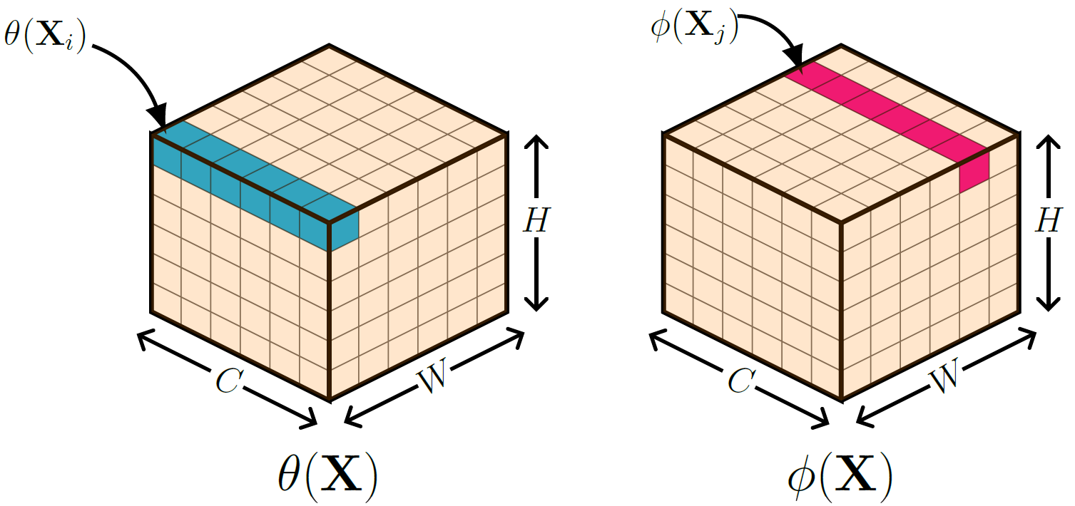
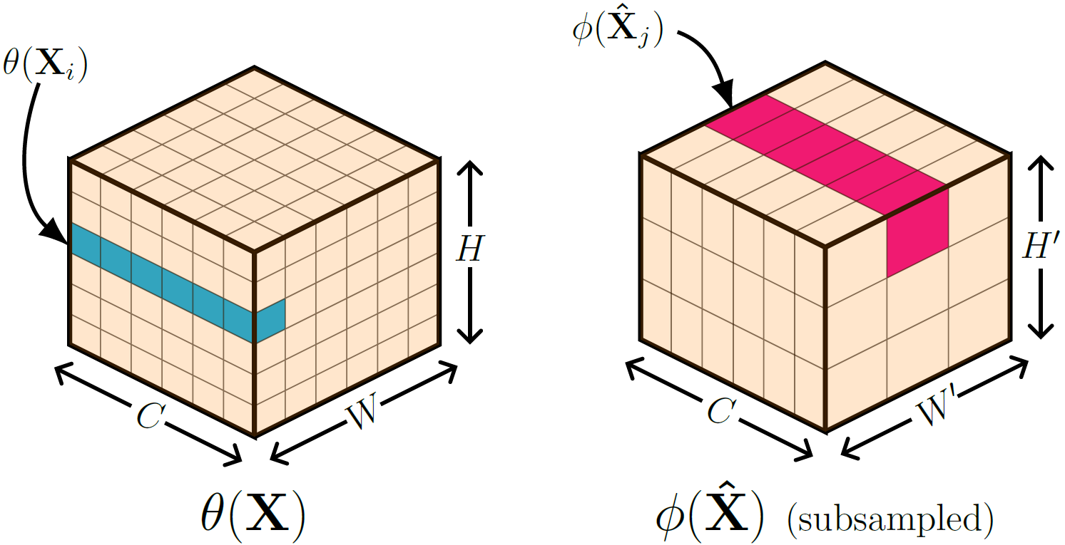
Figure 2: Pixel strips of embedded versions of $\mathbf{X}$ with $C$ channels, which are used to compute the unsubsampled kernel entry $\omega(\mathbf{X}_{i},\mathbf{X}_{j})$ (left) and the subsampled version of the kernel entry $\omega(\mathbf{X}_{i},\mathbf{\hat{X}}_{j})$ (right).

The term $\textstyle\sum_{j}\omega(\mathbf{X}_{i},\mathbf{X}_{j})$ is a normalizing factor. For the sake of simplicity, and for easier gradient computations, as suggested in [39], we choose this factor to be $\mathscr{N}$, where $\mathscr{N}=H\times W$ is the number of pixel strips in the input $\mathbf{X}$. For instance, in Figure 2, the number of pixel strips is $36$ for a $6\times 6$ image. Without this normalizing factor, the computations might blow up for inputs of larger sizes.

After the normalization, a $1\times 1$ convolution $\mathcal{K}_{1}$ is applied, along with ReLU and batch normalization, and then the result is added to the pixel strip of the original input, i.e. $\mathbf{X}_{i}$. Instead of simply discretizing the PIDE (equations (9) and (10)) using the forward Euler scheme, this computation is iteratively repeated several times, as shown in Figure 3. This allows us to extract more nonlocal information from the dataset.

Figure 3: The two-stage computation of a Nonlocal Block with skip connections.

The advantage of this multi-stage operation is that one can perform nonlocal operations several times, which widens the field-of-view of the network further, but the kernel $\omega$ is computed only once at the start, which saves computational time and effort. At the same time, one cannot have too many stages in one nonlocal block because, for instance, after Stage 5, we have the output $\mathbf{B}_{5}$, but the pre-computed kernel would fail to characterize the affinity between pairs of pixel strips of the features properly since the features would change quite a bit after each stage (see Section 5.2). Here, we restrict ourselves to a two-stage forward propagation, i.e. we repeat the computation twice.

It is important to note that this nonlocal block differs from the one suggested in [37] because, as shown in Figure 3, it contains identity skip connections. Similar to skip connections in ResNets, which have performed well for deep networks, skip connections in the nonlocal block are introduced to make sure that the nonlocal block does not impede the flow of information, which would force the network to perform worse. The experiments in Section 5.1 confirm this, showing that including skip connections in the nonlocal computations can be beneficial. This way, in the presence of nonlocal blocks, the network at least does not deliver a worse performance than a network without the nonlocality in the worst case. The exact details of how the tensors are dealt with and propagated forward in the nonlocal block are shown in SM3 in the supplementary material.

4.3 Fractional Laplacian operator $(-\Delta)^{s}$

As discussed before, the fractional Laplacian operator (11) can be seen as a special case of the nonlocal diffusion operator with kernel $\omega(\mathbf{x},\mathbf{y})=|\mathbf{x}-\mathbf{y}|^{-(n+2s)}$. Thus, the discretization can follow a similar procedure. In this case, we have the two-stage forward propagation

(19) $$\begin{aligned} \mathbf{[}\mathbf{B}_{1}]_{i}&=\mathbf{X}_{i}+h\,\mathcal{K}_{1}\Bigg{[}\displaystyle\frac{c_{n,s}}{\displaystyle\sum_{j}\omega(\mathbf{X}_{i},\mathbf{X}_{j})}\,{{\sum}}_{j}\frac{\lambda}{\big{\|}\theta(\mathbf{X}_{i})-\phi(\mathbf{X}_{j})\big{\|}^{n+2s}_{2}}(\mathbf{X}_{i}-\mathbf{X}_{j})\Bigg{]},\\ [\mathbf{B}_{2}]_{i}&=\mathbf{X}_{i}+h\,\mathcal{K}_{2}\Bigg{[}\displaystyle\frac{c_{n,s}}{\displaystyle\sum_{j}\omega(\mathbf{X}_{i},\mathbf{X}_{j})}\,{{\sum}}_{j}\frac{\lambda}{\big{\|}\theta(\mathbf{X}_{i})-\phi(\mathbf{X}_{j})\big{\|}^{n+2s}_{2}}\Big{(}[\mathbf{B}_{1}]_{i}-[\mathbf{B}_{1}]_{j}\Big{)}\Bigg{]},\end{aligned}$$

where $\theta$ and $\phi$ are again $1\times 1$ convolutional embeddings, $\|\cdot\|_{2}$ is the $L^{2}$ norm, $0<s<1$, and $\lambda>0$ is a scaling constant that is used to have greater control over the diffusion kernel. A small value of $\lambda$ leads to a weak interaction between the different pixel strips, whereas a large value of $\lambda$ damps the signal quickly. The rest of the expression is implemented in a similar fashion, with normalizing constant $\mathscr{N}$, etc (see Section SM3 in the supplementary material for further details). The forward propagation of the features through this 2-stage process can be again seen as a discretization of an underlying PIDE (equation (10) with $\mathcal{O}=\mathcal{L}$).

Besides, we have a singularity in the kernel if the embeddings of the pixel strips, i.e. $\theta(\mathbf{X}_{i})$ and $\phi(\mathbf{X}_{j})$, are the same. From Section SM2 in the supplementary material, we know that there is no net contribution to the integral when $\mathbf{y}\to\mathbf{x}$. Hence we just perform a safe divide, i.e. the kernel entry $\omega(\mathbf{X}_{i},\mathbf{X}_{j})=\frac{\lambda}{\big{\|}\theta(\mathbf{X}_{i})-\phi(\mathbf{X}_{j})\big{\|}^{n+2s}_{2}}$ is replaced with 0 if the denominator turns out to be zero.

4.4 Inverse fractional Laplacian operator $(-\Delta)^{-s}$

The inverse fractional Laplacian operator for $0<s<n/2$, defined by equation (14), can be discretized in a similar fashion using a two-stage method with skip connections, i.e.

(20) $$\begin{aligned} \mathbf{[}\mathbf{B}_{1}]_{i}&=\mathbf{X}_{i}+h\,\mathcal{K}_{1}\Bigg{[}\displaystyle\frac{c_{n,-s}}{\displaystyle\sum_{j}\omega(\mathbf{X}_{i},\mathbf{X}_{j})}\,{{\sum}}_{j}\frac{\lambda}{\big{\|}\theta(\mathbf{X}_{i})-\phi(\mathbf{X}_{j})\big{\|}^{n-2s}_{2}}\,\mathbf{X}_{j}\Bigg{]},\\ [\mathbf{B}_{2}]_{i}&=\mathbf{X}_{i}+h\,\mathcal{K}_{2}\Bigg{[}\displaystyle\frac{c_{n,-s}}{\displaystyle\sum_{j}\omega(\mathbf{X}_{i},\mathbf{X}_{j})}\,{{\sum}}_{j}\frac{\lambda}{\big{\|}\theta(\mathbf{X}_{i})-\phi(\mathbf{X}_{j})\big{\|}^{n-2s}_{2}}\,[\mathbf{B}_{1}]_{j}\Bigg{]}.\end{aligned}$$

For $s=n/2$, we have a $\log$ kernel (15), which is implemented in the nonlocal block as

(21) $$\begin{aligned} \mathbf{[}\mathbf{B}_{1}]_{i}&=\mathbf{X}_{i}+h\,\mathcal{K}_{1}\Bigg{[}\displaystyle\frac{c_{n}}{\displaystyle\sum_{j}\omega(\mathbf{X}_{i},\mathbf{X}_{j})}\,{{\sum}}_{j}\bigg{(}-2\lambda\log\bigg{(}\big{\|}\theta(\mathbf{X}_{i})-\phi(\mathbf{X}_{j})\big{\|}_{2}\bigg{)}-\gamma\bigg{)}\,\mathbf{X}_{j}\Bigg{]},\\ [\mathbf{B}_{2}]_{i}&=\mathbf{X}_{i}+h\,\mathcal{K}_{2}\Bigg{[}\displaystyle\frac{c_{n}}{\displaystyle\sum_{j}\omega(\mathbf{X}_{i},\mathbf{X}_{j})}\,{{\sum}}_{j}\bigg{(}-2\lambda\log\bigg{(}\big{\|}\theta(\mathbf{X}_{i})-\phi(\mathbf{X}_{j})\big{\|}_{2}\bigg{)}-\gamma\bigg{)}\,[\mathbf{B}_{1}]_{j}\Bigg{]}.\end{aligned}$$

For the case $0<s<n/2$, the kernel entry is again replaced with zero, in case the denominator happens to be zero. For the case $s=n/2$, if the term $\log\big{(}\|\theta(\mathbf{X}_{i})-\phi(\mathbf{X}_{j})\|_{2}\big{)}$ turns out to be undefined, the term is then replaced by $-\frac{\gamma}{2\lambda}$ so that it does not contribute to the overall sum.

These two operators are different from the previous two discussed in this section. While for the diffusion-like operators, the kernel is integrated with the term $\mathbf{X}_{j}-\mathbf{X}_{i}$ (and $[\mathbf{B}_{1}]_{j}-[\mathbf{B}_{1}]_{i}$), for these two operators, we have the term $\mathbf{X}_{j}$ (and $[\mathbf{B}_{1}]_{j}$) only. This is reflected in the performance of the overall network, as we will see in Section 5.1. The computations and forward propagations of the tensors for these two nonlocal blocks with and without subsampling are treated in a similar fashion as discussed before (see Figure SM2 in the supplementary material).

The PIDE-based nonlocal blocks discussed here have several advantages over other layers in the neural network. Firstly, it is clear that, for all the operators introduced here, the pixel strips’ values of the nonlocal block output depend on each pixel strip of the input tensor. This block is also different from a fully-connected layer because it computes activations based on relationships between different regions of the image, and these long-range dependencies are a function of the input data. This is different in a fully-connected layer, where the relationship is established using trainable weights. Secondly, a fully-connected layer can usually only be added at the end of the network due to computational cost reasons, and the local information is lost by flattening the image. On the other hand, the nonlocal block can be added anywhere in the network, and it preserves the 2D structure of images. Besides, the output and input shapes of this implementation are the same. Therefore, this block can be plugged into any neural network architecture associated with computer vision to accelerate the communication of information across pixels.

Note furthermore that the analogy to a Verlet time-discretization of a PIDE system can again easily be deduced as in Section 4.2. More specifically, the $\operatorname{Diff}$ operator in (18) and its implicit application in (17) just need to be substituted by the identity operator to obtain the corresponding systems for this case.

4.5 Regularization

The weight-decay or $L_{2}$ regularization will be used in our experiments. It penalizes large weights in the hidden layers of the network and is equivalent to the well-known Tikhonov regularization. Let $\mathbf{K}$ denote some (convolutional) weights of the network, then the $L_{2}$ regularizer is given by

(22) $$R_{1}(\mathbf{K})=\frac{\alpha_{1}}{2}\|\mathbf{K}\|_{F}^{2},$$

where $\|\cdot\|_{F}$ represents the Frobenius norm, and $\alpha_{1}$ is the regularization hyperparameter that controls the trade-off between larger and smaller trainable weights (see Section SM4).

For a stable forward propagation, we would ideally want the weight matrices $\mathbf{K}(t)$ to change smoothly with time, i.e. we would like convolution weights to be piecewise smooth in time. To this end, as suggested in [4], we use weight smoothness decay in combination with $L_{2}$ regularization. The smooth weight decay can be written as

(23) $$R_{2}(\mathbf{K})=\alpha_{2}\,h\sum_{j=1}^{N-1}\sum_{k=1}^{2}\bigg{\|}\frac{\mathbf{K}_{j,k}-\mathbf{K}_{j+1,k}}{h}\bigg{\|}_{F}^{2},$$

where $h$ is the step size, $\alpha_{2}$ is again a hyperparameter (see Section SM4), and $j$ represents each time step or each block of the PDE-based neural network. Here it is assumed that there are two convolution layers/weights $\mathbf{K}_{1}$ and $\mathbf{K}_{2}$ in each block/time step (in Hamiltonian blocks, for example). Because of the unique nature of nonlocal blocks, the weight smoothness decay is only applied to the normal blocks and not to the nonlocal blocks, whereas $L_{2}$ weight decay is applied to all the convolutional network weights. Both regularization terms are then added to the objective function (2), which the optimizer tries to then minimize.

4.6 Further implementation details

After the starting layer of $3\times 3$ convolutions, the original Hamiltonian network consists of 3 Units [4] with $m$ Hamiltonian blocks each. Average pooling with pool size 2 is used to decrease the size of the feature map between the Units, followed by $1\times 1$ convolution (with ReLU) instead of zero-padding to increase the number of channels. The convolutions within each block are all $3\times 3$ convolutions with spatial zero-padding to maintain feature map size. Further implementation details regarding the choice of hyperparameters etc. can be found in the supplementary material (Section SM4).

The nonlocal block is then added after the second block in each Unit, and this network is trained and tested on several image classification benchmark datasets, such as CIFAR-10, CIFAR-100 [19] and STL-10 [5]. The networks are also used for the semantic segmentation task in autonomous driving. To this end, the BDD100K dataset [40] is used, which is a large-scale dataset of visual driving scenes. The resolution of each image in this dataset is $1280\times 720$. To demonstrate the performance for the segmentation task, we use small networks, and therefore we resize the images to a resolution of $160\times 90$. This is done by removing every second row and column from each image and performing the same operation iteratively on the resulting image.

For training with CIFAR-10 and CIFAR-100, the mini-batch size is kept at 100. The per-pixel mean from the input image is subtracted before training [20], and the means of the training data are used to perform per-pixel mean subtraction on the test data. Common data augmentation techniques [22] are performed, such as padding 4 zeros around the image, followed by random cropping and random horizontal flipping. This makes the network more robust and helps it to generalize better. At the end of the network, before the fully-connected layer, we have an average pooling layer with a pool size of 2 (Figure 1). For subsampling within the nonlocal block, max-pooling is performed with a pool size of 2, i.e. $2\times 2$ patches of the image are used to compute the affinity kernel $\omega$.

For the STL-10 dataset, the mini-batch size is 50. The same preprocessing and data augmentation techniques are used but with a padding of 12 zeros around the image before cropping, instead of 4, because the images in the STL-10 dataset are significantly larger. At the end of the network, before the fully-connected layer, we have an average pooling layer with pool size 8. For subsampling within the nonlocal block, max-pooling is performed with a pool size of 4 in this case.

For the segmentation task with the BDD100K dataset, the mini-batch is of size 8. This value is intentionally kept small to avoid a large memory footprint due to the kernel computation and the relatively high image resolution. For the data augmentation, the per-pixel mean subtraction is performed, and then the image is randomly flipped horizontally. In a usual neural network for semantic segmentation tasks, the image is subsampled several times and then upsampled again to get a high-dimensional output. We use a simple architectural design here, i.e. the pooling layers that are shown in Figure 1 are left out. This way, the spatial dimensions of the image are maintained. At the end of the network, instead of a fully-connected layer, the output of the last unit is passed through a $1\times 1$ convolutional layer with 20 filters, which gives us the prediction of each of the pixels in the image. For subsampling within the nonlocal block, max-pooling is performed with a pool size of 3.

5 Numerical Experiments

We will denote the networks with the nonlocal blocks as nonlocal Hamiltonian networks, and the one without the nonlocality is just called Hamiltonian network. Each experiment is run five times with different random seeds, and the median test accuracy is reported in each case. In [4], the smallest Hamiltonian network proposed is a network with 74 layers, with 6 Hamiltonian blocks in each of the three Units (6-6-6). The initial convolutional layer has 32 filters, and the number of channels in each Unit is {32, 64, 112}. Such architectures with three Units have been used in ResNets and its variants, and have become a common blueprint for a well-performing CNN. We stick to the simple (6-6-6) architecture for our experiments. The last Unit intentionally has 112 channels to make sure that the resulting network is comparable to the baseline ResNet-44, in terms of the number of trainable parameters.

5.1 Training on benchmark datasets

Firstly, the nonlocal Hamiltonian networks are tested on the benchmark datasets CIFAR-10, CIFAR-100 and STL-10. The original Hamiltonian network, ResNet-44 and PreResNet-20 [17] are used as baseline networks for comparison and are trained on each of the three datasets. The main results with the test accuracies are shown in Table 1. The best result for each benchmark dataset is marked in boldface.

Table 1: Test accuracies on benchmark datasets for different nonlocal Hamiltonian networks.

Network	CIFAR-10		CIFAR-100		STL-10
	Params (M)	Acc. (%)	Params (M)	Acc. (%)	Params (M)	Acc. (%)
ResNet-44	$0.66$	$92.64$	$0.66$	$69.51$	$0.66$	$75.79$
PreResNet-20	$0.57$	$92.35$	$0.59$	$71.07$	$0.57$	$77.39$
Hamiltonian-74	$0.50$	$92.75$	$0.67$	$70.38$	$0.50$	$79.95$
Nonlocal diffusion $\mathcal{L}$	$0.56$	$\mathbf{93.27}$	$0.72$	$71.81$	$0.55$	$\mathbf{82.62}$
Pseudo-differential $(-\Delta)^{1/2}$		$93.21$		$\mathbf{71.84}$		$81.88$
Pseudo-differential $(-\Delta)^{-1/2}$		$93.08$		$71.24$		$81.56$
Pseudo-differential $(-\Delta)^{-1}$		$92.88$		$71.25$		$80.73$

The figures in Table 1 show that all of the nonlocal Hamiltonian networks perform better on the benchmark datasets than the baseline networks. They also have fewer parameters than the baseline networks of ResNet and PreResNet networks (for CIFAR-10 and STL-10). The nonlocal diffusion $\mathcal{L}$ network performs the best, closely followed by the pseudo-differential $(-\Delta)^{1/2}$ network, which can be seen as a special case of the nonlocal diffusion operator, as pointed out in Section 3.2. The inverse Laplacian operator $(-\Delta)^{-1}$ with the $\log$ kernel performs the worst, but it nevertheless outperforms the baseline networks. Besides, the accuracies of our networks are rather comparable to that of ResNet-56 and ResNet-110 and not to ResNet-44 (see [16]). This reiterates the fact that the nonlocal connections and their larger receptive fields somewhat compress the ResNet-like architectures. These connections partially alleviate the necessity to have very deep networks, and hence, we can save training time by training shallower networks with nonlocal blocks in them.

The nonlocal diffusion network performs better than the one proposed in [37], which did not have any skip connections in the nonlocal block. This suggests that introducing skip connections within the nonlocal block makes sure that the network learns only the update (or the residual) made to the identity function, and hence avoids any impedance when the information travels through the nonlocal block.

The nonlocal diffusion $\mathcal{L}$ network and the pseudo-differential $(-\Delta)^{1/2}$ network perform comparatively better than the other two proposed neural networks. This is possibly because of the difference term $[u(\mathbf{x})-u(\mathbf{y})]$ (and [$u(\mathbf{y})-u(\mathbf{x})$]). When computing each pixel in the output feature map, this term compares and computes the relative differences between the neighboring pixel values of the input feature map, whereas the operator $(-\Delta)^{-1/2}$ just computes a weighted sum of $u(\mathbf{y})$ (see Definition 3.4). Also, we see the biggest increase in accuracy for the STL-10 dataset. This is due to the fact that the images in this dataset are relatively larger than the ones in CIFAR-10/100, and therefore the nonlocality plays a more vital role in widening the receptive field of the network, which enables direct communication between pixels on opposite ends of the image. As an example, the test accuracy curves (till the 160th epoch) for the nonlocal diffusion network with each of the three datasets are shown in Figure 4. The Hamiltonian-74 network is used for comparison since it has the best performance out of all the three baseline networks.

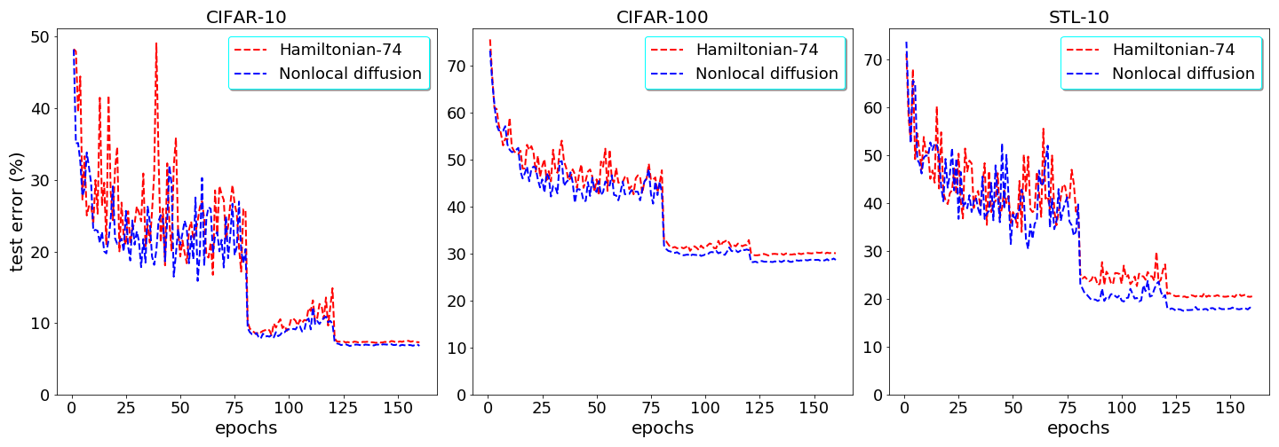
Figure 4: Test accuracy curves for the nonlocal diffusion $\mathcal{L}$ network in comparison to the original Hamiltonian network.

The nonlocal Hamiltonian networks can actually achieve better results for the STL-10 dataset. With a larger step size $h$, around $84\%$-$84.5\%$ test accuracy on STL-10 can be attained. For example, the pseudo-differential $(-\Delta)^{1/2}$ network was trained with a higher value of $h$, namely $h=0.15$, and it achieved a median test accuracy of $84.12\%$. The value of $h$ is intentionally kept low because, as pointed out in [41], a small $h$ encourages the model to have smaller weights. A model with larger weights tends to suffer from overfitting. Such models are also vulnerable to adversarial attacks.

It has been seen that although the pseudo-differential $(-\Delta)^{1/2}$ network performed slightly worse than the nonlocal diffusion network on the benchmark datasets (Section 5.1), it is at times more robust to noise and perturbations [13] than the nonlocal diffusion and Hamiltonian networks. This shows that a higher test accuracy of a network does not automatically mean more robustness to noise. The experiments have also shown that the nonlocal Hamiltonian networks, on average, need lesser training data to learn the features in the dataset and to achieve a certain generalization power.

5.2 Multi-stage nonlocal blocks

The discretizations of the nonlocal operators relate to a 2-stage computation (Figure 3). To see the effect of the number of stages in the nonlocal block, the nonlocal diffusion network with four stages is taken as an example and is trained on the datasets. The results are shown in Table 2.

Table 2: Test accuracies on benchmark datasets for the nonlocal diffusion $\mathcal{L}$ network with different number of stages in the nonlocal block.

# Stages	CIFAR-10		CIFAR-100		STL-10
	Params (M)	Acc. (%)	Params (M)	Acc. (%)	Params (M)	Acc. (%)
2	0.56	93.27	0.72	71.81	0.55	82.62
4	0.59	93.09	0.76	71.25	0.59	81.36

The figures indicate that too many stages in the nonlocal block damp the signal in the network, and hence, the network performs worse or at least does not perform any better than the network with a 2-stage nonlocal block. This is in line with the observations made in [37]. Operators similar to the inverse fractional Laplacian also suffer from instabilities if the number of stages is increased (see [37]). Therefore, although a nonlocal operation of this kind improves performance when the number of stages is kept low, overusing the nonlocal operation can lead to a lossy network.

5.3 Semantic segmentation on BDD100K

The aim of semantic segmentation is to predict the class of each pixel and thereby partition the image into different image classes or objects. This gives us an idea of where the object is present in the image and which pixels belong to it. This is of paramount importance, for example, for self-driving cars because the position and type of the object in front are necessary inputs to any self-driving algorithm.

The nonlocal Hamiltonian networks are used to segment images from the BDD100K dataset [40], which consists of images with everyday driving scenarios. An example of an image, along with its segmentation mask, is provided in Figure 5. Our aim here is to show the increase in performance due to the presence of nonlocal connections and not to challenge the state-of-the-art networks. Therefore, we employ simple architectures with no pooling layers to maintain the spatial dimension of the feature maps, and we work with smaller image resolutions, as mentioned in Section 4.6.

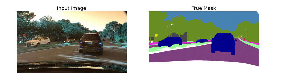
Figure 5: Input images and corresponding labels from Berkeley DeepDrive (BDD100K) dataset for the semantic segmentation task [40].

Table 3: Pixel accuracies and meanIoU for the semantic segmentation task on the BDD100K dataset using the nonlocal Hamiltonian networks.

Network	BDD100K
	Params (M)	P. Acc. (%)	mIoU (%)
ResNet-44	$0.66$	83.50	63.42
PreResNet-20	$0.57$	77.86	52.12
Hamiltonian-74	$0.49$	84.47	64.40
Nonlocal diffusion $\mathcal{L}$	$0.54$	84.80	$\mathbf{67.01}$
Pseudo-differential $(-\Delta)^{1/2}$		$\mathbf{85.24}$	66.71
Pseudo-differential $(-\Delta)^{-1/2}$		85.21	66.52
Pseudo-differential $(-\Delta)^{-1}$		84.95	66.26

To evaluate the performance, two metrics will be used. The first one is the pixel accuracy. The second metric that we use is the Intersection-over-Union (IoU) metric (or the Jaccard index). This is calculated on a per-class basis, and the mean is then taken over all the classes, which gives us the meanIoU (mIoU) metric. The results for the proposed neural networks can be seen in Table 3. When we consider the pixel accuracy and the mIoU metric, the nonlocal Hamiltonian networks perform better than the baseline networks. The nonlocal Hamiltonian networks’ metric values are very close to each other. We see that the nonlocal Hamiltonian networks have a performance gain of around 2–2.5 mIoU percentage points when we compare it to the original Hamiltonian network and around 3–3.5 mIoU percentage points when we compare it to ResNet-44. To make sure that the networks actually learn to segment the images from driving scenes into semantically meaningful parts, we look at the predictions made by the networks. Figure 6 shows the true label of a test image (with a taxi) and the different predictions made by some of the networks discussed above.

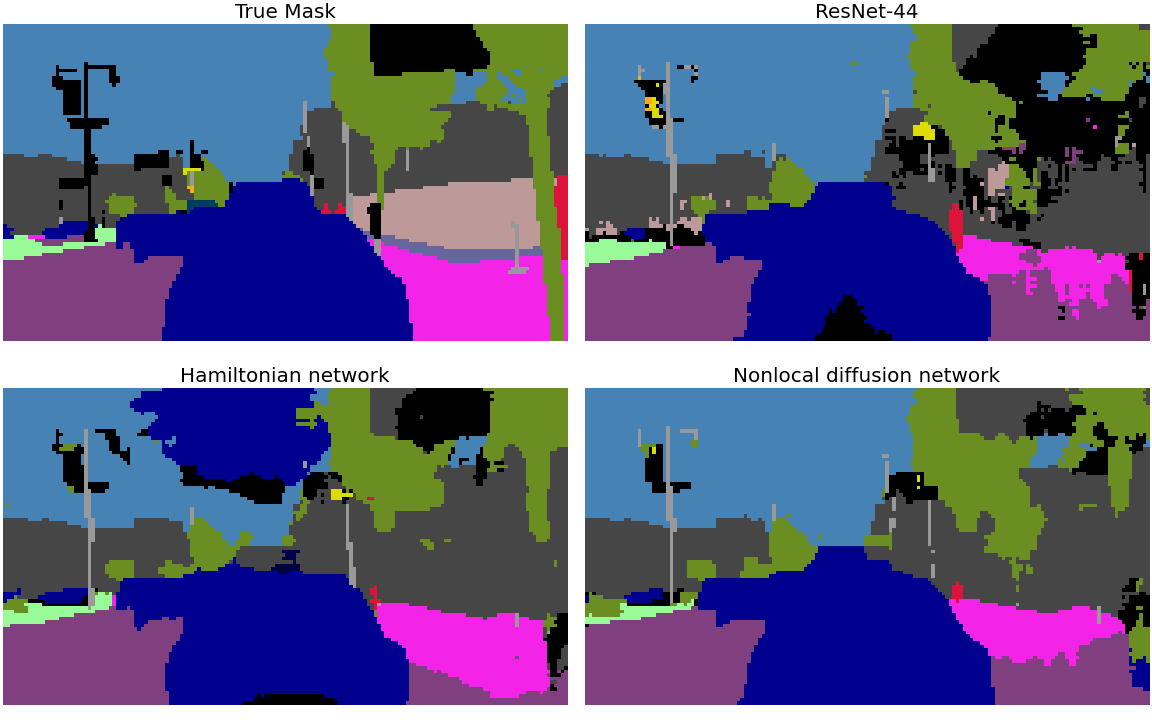
Figure 6: The true labels/masks of a test image from the BDD100K dataset and the predictions made by the different networks.

The results discussed here can be improved by performing segmentation using encoder-decoder models like U-Net [27] or data augmentation techniques, which we did deliberately not use here to completely focus on the comparison of the networks architectures themselves.

6 Computational cost and forward propagation stability

6.1 Computational cost of the nonlocal blocks

Table 4: Number of floating-point operations for each of the networks when trained on the image classification benchmark datasets.

Network	CIFAR-10	CIFAR-100	STL-10
	FLOPs (M)	FLOPs (M)	FLOPs (M)
ResNet-44	98.3	98.3	879.5
Hamiltonian-74	159.6	159.9	1432.5
Nonlocal diffusion $\mathcal{L}$	192.9	193.2	2003.7
Pseudo-differential $(-\Delta)^{1/2}$	193.4	193.7	2012.5
Pseudo-differential $(-\Delta)^{-1/2}$	193.2	193.5	2011.0
Pseudo-differential $(-\Delta)^{-1}$	193.6	193.9	2019.5

The nonlocal blocks come with a computational cost that needs to be taken into consideration while inserting them into any neural network. The number of FLOPs (multiply-adds) associated with the proposed networks for the image classification task are shown in Table 4. To ensure the stability of the forward propagation, we can observe that the Hamiltonian-74 network has roughly 1.5 times more FLOPs than the traditional ResNet-44. Also, the ResNets generally have only two convolutional layers in a Residual block. In comparison, Hamiltonian blocks have 2 convolutions and 2 transposed convolutions, which explains the higher number of FLOPs. The nonlocal blocks by themselves add only little extra floating-point operations for CIFAR-10 and CIFAR-100 but nevertheless help the networks achieve better accuracy on the benchmark datasets. For the effect of subsampling on the computational costs for STL-10 computations, see section SM5 in the supplementary material.

6.2 Stability of the PIDE-based forward propagation

It is crucial that the newly introduced PIDE-based nonlocal block does not introduce any instabilities in the forward propagation. If it did, then it would nullify the advantage of the PDE-based Hamiltonian network having the stability of the forward propagation. The spectral norms of the weight matrices have a major role to play in this regard. To investigate this, we look at the spectral nature of the weights in the nonlocal block.

Other than the embeddings $\theta$ and $\phi$, the nonlocal block has two $1\times 1$ convolutional layers $\mathcal{K}_{1}$ and $\mathcal{K}_{2}$ for the two stages. For the four nonlocal Hamiltonian networks used in Section 5.1, the weights of the convolution layers have the dimensions $\mathcal{K}_{1,2}\in\mathbb{R}^{32\times 32}$, $\mathcal{K}_{1,2}\in\mathbb{R}^{64\times 64}$, $\mathcal{K}_{1,2}\in\mathbb{R}^{112\times 112}$, and they belong to the three Units of the network, respectively. The outputs of these transformations are the feature maps that are used later on in other blocks of the network. Thus, we look at the eigenvalues of these matrices to see how the features are transformed by these trainable weights. Figure 7 shows the real parts of the eigenvalues of the weight matrices $\mathcal{K}_{1}$ and $\mathcal{K}_{2}$ in each Unit of the nonlocal diffusion network while training on STL-10. The real parts of the eigenvalues for the other nonlocal Hamiltonian networks can be found in the supplementary material.

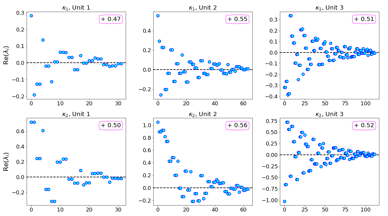
Figure 7: Real parts of the eigenvalues of weight matrices $\mathcal{K}_{1}$, $\mathcal{K}_{2}$ in the nonlocal block placed in each Unit of the nonlocal diffusion $\mathcal{L}$ network while training on STL-10.

The plots show that the real parts of the eigenvalues of the trainable weights are mostly very close to zero. The “$+$” sign in each plot indicates the fraction of eigenvalues that have positive real parts. In the ideal case, this value should stay close to 0.5. Too many eigenvalues with positive real parts would lead to amplification of the signal resulting in instabilities in the forward propagation. On the other hand, too many eigenvalues with negative real parts would lead to a lossy network. The plots for the nonlocal diffusion network are pretty symmetric. The plots for the pseudo-differential networks $(-\Delta)^{1/2}$, $(-\Delta)^{-1/2}$ and $(-\Delta)^{-1}$ (Figures SM3, SM4, and SM5 in the supplementary material) show that the real parts are slightly more asymmetrically distributed, which partly explains their relatively worse performance.

There is another way of looking at the properties of the transformations carried out by the trainable weight matrices $\mathcal{K}_{1}$ and $\mathcal{K}_{2}$. Let $\mathcal{K}\in\{\mathcal{K}_{1},\mathcal{K}_{2}\}$. Then the amplification or damping of the features by $\mathcal{K}\in\mathbb{R}^{n\times n}$ is mainly determined by the associated quadratic form $\mathbf{x}^{T}\mathcal{K}\mathbf{x}\in\mathbb{R}$, for $\mathbf{x}\in\mathbb{R}^{n}$. We can decompose $\mathcal{K}$ into a symmetric and an antisymmetric part

$$\mathcal{K}=\frac{\mathcal{K}+\mathcal{K}^{T}}{2}+\frac{\mathcal{K}-\mathcal{K}^{T}}{2}=\mathcal{K}_{s}+\mathcal{K}_{as}.$$

Then the quadratic form of $\mathcal{K}$ is given by $\mathbf{x}^{T}\mathcal{K}\mathbf{x}=\mathbf{x}^{T}\mathcal{K}_{s}\mathbf{x}$, where the quadratic form of the antisymmetric matrix $\mathcal{K}_{as}$ is zero. Therefore, the quadratic form of the symmetric part of $\mathcal{K}$, i.e. the quadratic form of $\mathcal{K}_{s}$, determines the spectral properties of the transformations. Since $\mathcal{K}_{s}$ is symmetric, the eigenvalues are all real.

Figure 8 shows the eigenvalues of the symmetric parts of the weight matrices $\mathcal{K}_{1}$ and $\mathcal{K}_{2}$ in each Unit in the nonlocal diffusion network while training on STL-10. The eigenvalues of the symmetric parts for the other nonlocal Hamiltonian networks can be found in the supplementary material (Figures SM6, SM7, and SM8). The “$+$” sign in each plot indicates the fraction of positive eigenvalues. The plots show that most of the eigenvalues are well-bounded and symmetric, unlike in the case of the network suggested in [39], where the eigenvalues of the symmetric part are significantly larger when multiple stages are added to the nonlocal block, as shown in [37]. This well-boundedness of the eigenvalues makes the task of the optimizer easier, which leads to faster convergence.

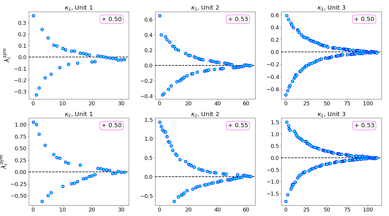
Figure 8: Eigenvalues of the symmetric parts of weight matrices $\mathcal{K}_{1}$, $\mathcal{K}_{2}$ in the nonlocal block placed in each Unit of the nonlocal diffusion $\mathcal{L}$ network while training on STL-10.

7 Conclusion

The proposed neural networks achieve better accuracy than the original Hamiltonian model and the widely-used state-of-the-art ResNets. Due to an appropriate combination of local and nonlocal information, the network gets a more comprehensive view of each example during training. The nonlocal diffusion $\mathcal{L}$ network and the pseudo-differential $(-\Delta)^{s}$ network perform slightly better than the other two proposed networks. Moreover, the PIDE-based nonlocal block maintains the 2D structure of the images and has the same output shape as the input shape. Hence, they can be seamlessly inserted into any network. This can be useful if a neural network is to be trained and tested on a dataset that warrants nonlocal connections between the regions of the image. Using spectral properties of the transformation matrices, we showed that the nonlocal blocks do not destabilize the original Hamiltonian network in any way, and consequently, the stability of the forward propagation is still preserved.

References

- [1] U. Ascher, Numerical Methods for Evolutionary Differential Equations, Society for Industrial and Applied Mathematics (SIAM), 2008.
- [2] A. Buades, B. Coll, and J.-M. Morel, A non-local algorithm for image denoising, in 2005 IEEE Computer Society Conference on Computer Vision and Pattern Recognition (CVPR’05), vol. 2, IEEE, 2005, pp. 60–65.
- [3] M. Caputo, Linear models of dissipation whose Q is almost frequency independent—II, Geophysical Journal International, 13 (1967), pp. 529–539.
- [4] B. Chang, L. Meng, E. Haber, L. Ruthotto, D. Begert, and E. Holtham, Reversible architectures for arbitrarily deep residual neural networks, in 32nd AAAI Conference on Artificial Intelligence, 2018.
- [5] A. Coates, A. Ng, and H. Lee, An analysis of single-layer networks in unsupervised feature learning, in Proceedings of the 14th International Conference on Artificial Intelligence and Statistics, vol. 15, 2011, pp. 215–223.
- [6] R. Collobert and J. Weston, A unified architecture for natural language processing: Deep neural networks with multitask learning, in Proceedings of the 25th International Conference on Machine Learning (ICML), 2008, pp. 160–167.
- [7] R. Cont, Long range dependence in financial markets, in Fractals in Engineering, Springer, 2005, pp. 159–179.
- [8] E. Di Nezza, G. Palatucci, and E. Valdinoci, Hitchhiker’s guide to the fractional Sobolev spaces, Bulletin des Sciences Mathématiques, 136 (2012), pp. 521–573.
- [9] Q. Du, M. Gunzburger, R. Lehoucq, and K. Zhou, Analysis and approximation of nonlocal diffusion problems with volume constraints, SIAM Review, 54 (2012), pp. 667–696.
- [10] W. E, A proposal on machine learning via dynamical systems, Communications in Mathematics and Statistics, 5 (2017), pp. 1–11.
- [11] G. Gilboa and S. Osher, Nonlocal linear image regularization and supervised segmentation, Multiscale Modeling & Simulation, 6 (2007), pp. 595–630.
- [12] I. Goodfellow, Y. Bengio, and A. Courville, Deep Learning, MIT Press, 2016. http://www.deeplearningbook.org.
- [13] I. Goodfellow, J. Shlens, and C. Szegedy, Explaining and harnessing adversarial examples, in International Conference on Learning Representations (ICLR), 2015.
- [14] E. Haber and L. Ruthotto, Stable architectures for deep neural networks, Inverse Problems, 34 (2017).
- [15] K. He, G. Gkioxari, P. Dollár, and R. Girshick, Mask R-CNN, in 2017 IEEE International Conference on Computer Vision (ICCV), 2017, pp. 2980–2988.
- [16] K. He, X. Zhang, S. Ren, and J. Sun, Deep residual learning for image recognition, in 2016 IEEE Conference on Computer Vision and Pattern Recognition (CVPR), 2016, pp. 770–778.
- [17] K. He, X. Zhang, S. Ren, and J. Sun, Identity mappings in deep residual networks, in European Conference on Computer Vision (ECCV), Springer, 2016, pp. 630–645.
- [18] S. Ioffe and C. Szegedy, Batch normalization: Accelerating deep network training by reducing internal covariate shift, in Proceedings of the 32nd International Conference on Machine Learning (ICML), vol. 37 of Proceedings of Machine Learning Research, PMLR, 2015, pp. 448–456.
- [19] A. Krizhevsky, Learning multiple layers of features from tiny images, tech. report, University of Toronto, 2009.
- [20] A. Krizhevsky, I. Sutskever, and G. Hinton, ImageNet classification with deep convolutional neural networks, in Advances in Neural Information Processing Systems, 2012, pp. 1097–1105.
- [21] M. Kwaśnicki, Ten equivalent definitions of the fractional Laplace operator, Fractional Calculus and Applied Analysis, 20 (2017), pp. 7–51.
- [22] C.-Y. Lee, S. Xie, P. Gallagher, Z. Zhang, and Z. Tu, Deeply-supervised nets, in Artificial Intelligence and Statistics, 2015, pp. 562–570.
- [23] W. Luo, Y. Li, R. Urtasun, and R. Zemel, Understanding the effective receptive field in deep convolutional neural networks, in Advances in Neural Information Processing Systems, 2016, pp. 4898–4906.
- [24] R. Pascanu, T. Mikolov, and Y. Bengio, On the difficulty of training recurrent neural networks, in International Conference on Machine Learning (ICML), vol. 28, 2013, pp. 1310–1318.
- [25] T. Pohlen, A. Hermans, M. Mathias, and B. Leibe, Full-resolution residual networks for semantic segmentation in street scenes, in 2017 IEEE Conference on Computer Vision and Pattern Recognition (CVPR), 2017, pp. 3309–3318.
- [26] M. Renardy and R. Rogers, An Introduction to Partial Differential Equations, Springer Science & Business Media, 2006.
- [27] O. Ronneberger, P. Fischer, and T. Brox, U-Net: Convolutional networks for biomedical image segmentation, in International Conference on Medical Image Computing and Computer-Assisted Intervention (MICCAI), Springer, 2015, pp. 234–241.
- [28] L. Ruthotto and E. Haber, Deep neural networks motivated by partial differential equations, Journal of Mathematical Imaging and Vision, 62 (2020), pp. 352–364.
- [29] L. Silvestre, Regularity of the obstacle problem for a fractional power of the Laplace operator, Communications on Pure and Applied Mathematics, 60 (2007), pp. 67–112.
- [30] K. Simonyan and A. Zisserman, Very deep convolutional networks for large-scale image recognition, in International Conference on Learning Representations (ICLR), 2015.
- [31] J. Sirignano and K. Spiliopoulos, DGM: A deep learning algorithm for solving partial differential equations, Journal of Computational Physics, 375 (2018), pp. 1339–1364.
- [32] E. Stein, Singular Integrals and Differentiability Properties of Functions, vol. 2, Princeton University Press, 1970.
- [33] P. Stinga, Fractional powers of second order partial differential operators: Extension problem and regularity theory, PhD thesis, Universidad Autónoma de Madrid, 2010.
- [34] P. Stinga, User’s guide to the fractional Laplacian and the method of semigroups, Fractional Differential Equations, (2019), pp. 235–266.
- [35] P. Stinga and J. Torrea, Extension problem and Harnack’s inequality for some fractional operators, Communications in Partial Differential Equations, 35 (2010), pp. 2092–2122.
- [36] C. Szegedy, S. Ioffe, V. Vanhoucke, and A. Alemi, Inception-v4, Inception-ResNet and the impact of residual connections on learning, in 31st AAAI Conference on Artificial Intelligence, 2017.
- [37] Y. Tao, Q. Sun, Q. Du, and W. Liu, Nonlocal neural networks, nonlocal diffusion and nonlocal modeling, in Advances in Neural Information Processing Systems, 2018, pp. 496–506.
- [38] R. Vidal, J. Bruna, R. Giryes, and S. Soatto, Mathematics of deep learning, arXiv preprint arXiv:1712.04741, (2017).
- [39] X. Wang, R. Girshick, A. Gupta, and K. He, Non-local neural networks, in 2018 IEEE/CVF Conference on Computer Vision and Pattern Recognition (CVPR), 2018, pp. 7794–7803.
- [40] F. Yu, H. Chen, X. Wang, W. Xian, Y. Chen, F. Liu, V. Madhavan, and T. Darrell, BDD100K: A diverse driving dataset for heterogeneous multitask learning, in The IEEE Conference on Computer Vision and Pattern Recognition (CVPR), June 2020.
- [41] J. Zhang, B. Han, L. Wynter, K. Low, and M. Kankanhalli, Towards robust ResNet: A small step but a giant leap, in Proceedings of the 28th International Joint Conference on Artificial Intelligence, IJCAI-19, International Joint Conferences on Artificial Intelligence Organization, 7 2019, pp. 4285–4291.
- [42] D.-X. Zhou, Universality of deep convolutional neural networks, Applied and Computational Harmonic Analysis, 48 (2020), pp. 787–794.
- [43] D. Zügner, A. Akbarnejad, and S. Günnemann, Adversarial attacks on neural networks for graph data, in Proceedings of the 24th ACM SIGKDD International Conference on Knowledge Discovery & Data Mining, 2018, pp. 2847–2856.