Active matter in infinite dimensions: Fokker-Planck equation and dynamical mean-field theory at low density

Abstract

We investigate the behavior of self-propelled particles in infinite space dimensions by comparing two powerful approaches in many-body dynamics: the Fokker-Planck equation and dynamical mean-field theory. The dynamics of the particles at low densities and infinite persistence time is solved in the steady-state with both methods, thereby proving the consistency of the two approaches in a paradigmatic out-of-equilibrium system. We obtain the analytic expression for the pair distribution function and the effective self-propulsion to first order in the density, confirming the results obtained in a previous paper ALW19 and extending them to the case of a non-monotonous interaction potential. Furthermore, we obtain the transient behavior of active hard spheres when relaxing from equilibrium to the nonequilibrium steady-state. Our results show how collective dynamics is affected by interactions to first order in the density, and point out future directions for further analytical and numerical solutions of this problem.

I Introduction

The dynamics of active systems has become in the last years one of the most fertile research grounds in nonequilibrium statistical physics. This upsurge of interest stems from the emergence of collective behaviors whose phenomenology is deeply rooted in the intrinsic nonequilibrium nature of the dynamics VZ12pr ; CT15arcmp ; BDLLRVV16rmp . One of the most paradigmatic model of active matter is given by self-propelled particles, i.e. particles that are able to move individually without the need of interactions or thermal fluctuations, but rather driven by an internal self-propulsion giving them a characteristic velocity with typical persistence time. Even in absence of attractive or aligning interactions, it has been shown that these models can exhibit spectacular properties such as motility-induced phase separation (MIPS) TC08prl and local polar order CMBMP20prl ; Henkes20natcomm ; Szamel21epl . Several recent studies also started to investigate the dynamics of dense particle systems where the activity can be continuously increased, in order to assess the effect of activity on the glass transition and jamming BK13 ; FSB16sm ; bi2016motility ; BFS19jcp . A theoretical understanding of such systems strongly deals with their many-body nature, especially when considering the dynamics of dense phases. Indeed, in dense active systems, the difficulties and the need of approximations already needed to understand the behavior of equilibrium liquids Hansen combine with the inherently nonequilibrium nature of the dynamics.

The limit of large space dimensionality has gained attraction first in the field of simple liquids for its ability to capture the thermodynamics of dense phases restricting the analytical difficulties to the computation of the second-order virial coefficient FRW85 . The large-dimensional limit is a standard tool in statistical mechanics to study phase transitions ParisiBook , it has been then widely used to study the glass transition KW87 ; CKPUZ17 ; parisi2020theory . This framework allowed for the derivation of dynamical mean-field theory (DMFT): the main idea originated in the dynamics of strongly correlated electrons GKKR96 , and has been then applied to describe the microscopic, fluctuating dynamics of equilibrium liquids MKZ15 ; Sz17 , and later of general, nonequilibrium dynamics of particle systems AMZ19 ; AMZ19b . The equilibrium dynamical equations have recently been numerically solved MSZ20 , obtaining the force-force correlation kernels baity2019mean leading to the identification of a dynamical glass transition for hard and soft spheres interaction potential.

In another recent work, an approximate way to determine the steady-state many-body dynamics of self-propelled particles in infinitely many dimensions was presented ALW19 . Conversely from the DMFT approach, the dynamics has been described within the framework of kinetic theory (KT), with a proposed closure of the BBGKY hierarchy taking $1/d$ as the small parameter in perturbation theory. Under these assumptions, it has been shown for self-propelled hard spheres how the $n$-particle distribution function is determined by the pair distribution in the infinite-dimensional limit, leading to the derivation of: (i) the effective propulsion of individual particles, i.e. the actual speed of a tagged particle subject to active self-propulsion and repulsive interactions; (ii) the equation of state for the pressure $P$ of the active system, leading to the observation of MIPS as a spinodal transition when the pressure decreases with the density.

The above-mentioned study represents one of the first investigations on the dynamics of infinite-dimensional particle systems out of equilibrium, in a paradigmatic field such as active matter. In this paper, we compare the two approaches reproducing the results from KT in the DMFT framework, and apply both theories to solve the dynamics of sticky hard spheres at low densities and infinite persistence time - a framework that has been investigated in several recent studies stenhammar2014phase ; ALW19 ; Mo20sm ; Morse21pnas ; Agoritsas21jsm . We will show how the pair distribution function $g(r)$ and the density-dependent effective propulsion $v(\rho)$ can be analytically and consistently obtained in both cases. Furthermore, the analytical solution of DMFT equations includes as well the relaxation from a Boltzmann equilibrium state to a nonequilibrium steady state once activity is switched on, giving new insights into the structural properties of these systems.

The paper is organized as follows. Sec. II provides the basic definitions of the model and of its relevant parameters. In Sec. III.1, we derive the expression for the pair distribution function and the effective propulsion velocity by means of kinetic theory. In Sec. III.2, the same results are found by means of the dynamical mean-field theory in the steady state. In Sec. IV, we then reconsider the purely repulsive hard sphere case discussed in ALW19 , including the transient effects obtained by DMFT. We then summarize our findings and point out to possible next steps for future investigation.

II Definition of the model

We consider the dynamics of $N$ interacting $d$-dimensional self-propelled particles with equations of motion that read

$$\zeta\dot{\text{\bf x}}_{i}(t)=\text{\bf f}_{i}(t)-\sum_{j(\neq i)}\bm{\nabla}_{\text{\bf x}_{i}}V\left(\text{\bf x}_{i}(t)-\text{\bf x}_{j}(t)\right)\,.$$ (1)

In Eq.(1), motion is induced by (i) a self-propulsion force $\text{\bf f}_{i}(t)$ and (ii) pairwise conservative forces deriving from the potential $U\left(\text{\bf x}_{1},\dots\text{\bf x}_{N}\right)=\sum_{i<j}V\left(\text{\bf x}_{i}-\text{\bf x}_{j}\right)$. The pair potential is taken radially symmetric, $V\left(\text{\bf x}\right)=V(x)$ with $x=|\text{\bf x}|$. There exist different descriptions of the driving force, each of them corresponding to a particular model of self-propelled particles. In the following, we choose to work with run-and-tumble particles (RTPs) in which case the active force reads $\text{\bf f}_{i}(t)=v_{0}\text{\bf u}_{i}(t)$ with $\text{\bf u}_{i}(t)$ a unit vector randomly and uniformly reshuffled on the $(d-1)$-dimensional unit sphere with rate $\tau_{p}^{-1}$, thus yielding $\left\langle u_{i}^{\mu}(t)u_{j}^{\nu}(s)\right\rangle=\delta_{ij}\delta^{\mu\nu}\exp{\left(-|t-s|/\tau_{p}\right)}/d$. Note however that, as shown in ALW19 , the three standard models of self-propelled particles, i.e. RTPs, active Brownian particles and active Ornstein-Ulhenbeck particles, are equivalent in the limit where the space dimension $d$ is sent to infinity and the persistence time is large. In the present work, we study the dynamics Eq. (1) at low densities in the limit $d\rightarrow\infty$. We follow AMZ19 ; AMZ19b and take the infinite dimensional limit as follows:

• the pair potential is assumed to decay over a short length scale as $V(x)=\widehat{V}(h)$ with $h=d(x/\ell-1)$. The length scale $\ell$ can be viewed as the particle diameter; the rescaled gap $h$ accounts for the interparticle distance in the $d\rightarrow\infty$ limit. We then have $h<0$ for overlapping particles, and viceversa;

• the packing fraction $\varphi$ (or accordingly the number density $\rho$) is such that each particle interacts with $O(d)$ other particles, i.e. $\widehat{\varphi}=2^{d}\varphi/d=\rho\,\Omega_{d}\ell^{d}/d^{2}$ is kept finite with $\Omega_{d}$ the $d$-dimensional solid angle;

• the norm of the active drive is rescaled as $v_{0}=(\sqrt{2}d^{3/2}/\ell)\widehat{v}_{0}$. In Eq. (1), this equates the scaling of the norms of the conservative force and of the active force;

• the friction coefficient is rescaled as $\zeta=(2d^{2}/\ell^{2})\widehat{\zeta}$. In this scaling, the variations of the rescaled separation $h$ between two particles over finite time scales are $O(1)$;

• the times $t$ and $\tau_{p}$ are left unchanged.

We also remark that in this settings the equilibrium dynamics can be recovered in the limit $\tau_{p}\rightarrow 0$ by setting $\widehat{v}_{0}^{2}=\widehat{\zeta}T/\tau_{p}$. With this prescription, the active force becomes a thermal noise at temperature $T$ in the limit of vanishing persistence.

III Sticky spheres

III.1 Results from the Fokker-Planck equation

III.1.1 The two-body problem in the infinite dimensional limit

We start by addressing the dynamics of two interacting self-propelled particles. The interaction is carried through a spherically symmetric potential $V$ and both particles are subject to an external active drive. Following Eq. (1), their equations of motion read

$$\begin{split}\zeta\dot{\text{\bf x}}_{1}(t)&=v_{0}\text{\bf u}_{1}(t)-\bm{\nabla}_{\text{\bf x}_{1}}V\left(\text{\bf x}_{1}(t)-\text{\bf x}_{2}(t)\right)\,,\\ \zeta\dot{\text{\bf x}}_{2}(t)&=v_{0}\text{\bf u}_{2}(t)-\bm{\nabla}_{\text{\bf x}_{2}}V\left(\text{\bf x}_{2}(t)-\text{\bf x}_{1}(t)\right)\,,\end{split}$$ (2)

with $\text{\bf u}_{1}(t)$ and $\text{\bf u}_{2}(t)$ two independent run-and-tumble noises. We then introduce $\text{\bf r}=\text{\bf x}_{2}-\text{\bf x}_{1}$, the relative separation, and $P(\text{\bf r},\text{\bf u}_{1},\text{\bf u}_{2})$, the stationary state probability density associated to the process in Eq. (2). The latter obeys the following integro-differential equation

$$-v_{0}\left(\text{\bf u}_{2}-\text{\bf u}_{1}\right)\cdot\bm{\nabla}_{\text{\bf r}}P+2\bm{\nabla}_{\text{\bf r}}\cdot\left(P\bm{\nabla}_{\text{\bf r}}V(\text{\bf r})\right)+\frac{\zeta}{\tau_{p}}\left[\int\frac{\text{d}\text{\bf u}^{\prime}}{\Omega_{d}}P(\text{\bf r},\text{\bf u}^{\prime},\text{\bf u}_{2})+\int\frac{\text{d}\text{\bf u}^{\prime}}{\Omega_{d}}P(\text{\bf r},\text{\bf u}_{1},\text{\bf u}^{\prime})-2P(\text{\bf r},\text{\bf u}_{1},\text{\bf u}_{2})\right]=0\,,$$ (3)

where the terms between brackets account for the tumble dynamics of the active degrees of freedom $\text{\bf u}_{1}$ and $\text{\bf u}_{2}$. Taking advantage of the rotational symmetry of $P$ we introduce the variables

$$\begin{split}r&=|\text{\bf r}|\,,\\ w_{1}&=\left(\text{\bf u}_{1}\cdot\text{\bf r}\right)/r\,,\\ w_{2}&=\left(\text{\bf u}_{2}\cdot\text{\bf r}\right)/r\,,\\ z&=\text{\bf u}_{1}\cdot\text{\bf u}_{2}\,,\\ \end{split}$$ (4)

the use of which allows us to rewrite to Fokker-Planck equation in terms of four (instead of $3d$) coordinates as

$$\begin{split}0=&-v_{0}\left(w_{2}-w_{1}\right)\partial_{r}P-\frac{v_{0}}{r}\left[\left(1+w_{1}w_{2}-z\right)\left(\partial_{w_{2}}-\partial_{w_{1}}\right)P-\left(w_{2}^{2}\,\partial_{w_{2}}-w_{1}^{2}\,\partial_{w_{1}}\right)P\right]+\frac{2}{r^{d-1}}\partial_{r}\left(r^{d-1}V^{\prime}(r)P\right)\\ &+\frac{\zeta}{\tau_{p}}\left[\frac{\Omega_{d-2}}{\Omega_{d}}\frac{1}{\sqrt{1-w_{2}^{2}}}\int_{-1}^{1}\text{d}w_{1}^{\prime}\int_{w_{1}^{\prime}w_{2}-\sqrt{1-w_{2}^{2}}\sqrt{1-w_{1}^{\prime 2}}}^{w_{1}^{\prime}w_{2}+\sqrt{1-w_{2}^{2}}\sqrt{1-w_{1}^{\prime 2}}}\!\!\!\text{d}z^{\prime}P(r,w_{1}^{\prime},w_{2},z^{\prime})\left(1-w_{1}^{\prime 2}-\frac{z^{\prime 2}+w_{1}^{\prime 2}w_{2}^{2}-2z^{\prime}w_{1}^{\prime}w_{2}}{1-w_{2}^{2}}\right)^{\frac{d-4}{2}}\right.\\ &\left.+\frac{\Omega_{d-2}}{\Omega_{d}}\frac{1}{\sqrt{1-w_{1}^{2}}}\int_{-1}^{1}\text{d}w_{2}^{\prime}\int_{w_{1}w_{2}^{\prime}-\sqrt{1-w_{2}^{\prime 2}}\sqrt{1-w_{1}^{2}}}^{w_{1}w_{2}^{\prime}+\sqrt{1-w_{2}^{\prime 2}}\sqrt{1-w_{1}^{2}}}\!\!\!\text{d}z^{\prime}P(r,w_{1},w_{2}^{\prime},z^{\prime})\left(1-w_{2}^{\prime 2}-\frac{z^{\prime 2}+w_{2}^{\prime 2}w_{1}^{2}-2z^{\prime}w_{2}^{\prime}w_{1}}{1-w_{1}^{2}}\right)^{\frac{d-4}{2}}\right.\\ &\left.\vphantom{\left(1-w_{2}^{\prime 2}-\frac{z^{\prime 2}+w_{2}^{\prime 2}w_{1}^{2}-2z^{\prime}w_{2}^{\prime}w_{1}}{1-w_{1}^{2}}\right)^{\frac{d-4}{2}}}-2P(r,w_{1},w_{2},z)\right].\end{split}$$ (5)

The limit of infinite dimension $d\rightarrow\infty$ is then taken in Eq. (5) with:

$$\begin{split}&r=\ell\left(1+h/d\right)\,,\\ &w_{1}\rightarrow w_{1}/\sqrt{d}\,,\\ &w_{2}\rightarrow w_{2}/\sqrt{d}\,,\\ &z\rightarrow z/\sqrt{d}\,.\\ \end{split}$$ (6)

while keeping $h$, and the redefined $w_{1}$, $w_{2}$, $z$ fixed. The infinite dimensional limit of Eq. (5) is obtained to leading order in $d$ as:

$$\begin{split}&-\frac{\widehat{v}_{0}}{\sqrt{2}}\left(w_{2}-w_{1}\right)\,\partial_{h}P-\frac{\widehat{v}_{0}}{\sqrt{2}}\left(\partial_{w_{2}}-\partial_{w_{1}}\right)P+e^{-h}\partial_{h}\left(e^{h}\frac{\widehat{V}^{\prime}(h)}{\ell}P\right)\\ &+\frac{\widehat{\zeta}}{\tau_{p}}\left[\int_{-\infty}^{+\infty}\frac{\text{d}w_{1}^{\prime}\,\text{d}z^{\prime}}{2\pi}\exp{\left(-\frac{w_{1}^{\prime 2}}{2}-\frac{z^{\prime 2}}{2}\right)}P\left(h,w_{1}^{\prime},w_{2},z^{\prime}\right)\right.\\ &\left.+\int_{-\infty}^{+\infty}\frac{\text{d}w_{2}^{\prime}\,\text{d}z^{\prime}}{2\pi}\exp{\left(-\frac{w_{2}^{\prime 2}}{2}-\frac{z^{\prime 2}}{2}\right)}P\left(h,w_{1},w_{2}^{\prime},z^{\prime}\right)-2P\left(h,w_{1},w_{2},z\right)\right]=0\,.\end{split}$$ (7)

III.1.2 Analytical solution with infinite persistence

Equation (LABEL:eq:FP_dinf) can be solved analytically for certain classes of potentials in the ballistic limit $\tau_{p}\rightarrow\infty$. Beside providing nice analytical simplifications, this limit is conjectured to be of particular interest regarding the phase behavior of macroscopic systems of interacting active particles, see stenhammar2014phase for a discussion in $d=2$ and $d=3$ and ALW19 for a discussion in $d\rightarrow\infty$. At $\tau_{p}\rightarrow\infty$, only the relative speed $w=\left(w_{2}-w_{1}\right)/\sqrt{2}$ enters the game and

$$-\widehat{v}_{0}\left(w\partial_{h}P+\partial_{w}P\right)+e^{-h}\partial_{h}\left(e^{h}\frac{\widehat{V}^{\prime}(h)}{\ell}P\right)=0$$ (8)

with $P(h\rightarrow\infty,w)=1$ as a boundary condition. Note that similar first order equations also appear in the study of dilute passive colloids at high shear rate russel1991colloidal . The class of potentials we work with in the following is that of sticky-sphere potentials. These potentials have hard-sphere repulsion at $h<0$ while displaying an infinitely short ranged attractive well at $h=0^{+}$ and are vanishing at $h>0$. Such potentials are similar in spirit to the Baxter potential sometimes used as a model for passive colloids with short ranged attraction baxter1968percus . However, we make use of a slightly different mathematical construction of these sticky-sphere potentials. Indeed, the pairwise force, when attractive, must always be finite for the stationary state to be well-defined. Were this not to be true, then the two particles whose dynamics is given in Eq. (2) would never separate after a collision, the driving forces being unable to counterbalance the attractive force created by the potential. The sticky sphere potential is constructed as follows:

$$\widehat{V}(h)=\begin{cases}\widehat{v}_{0}\,w_{0}\left(\frac{\lambda}{2}h^{2}+h-\frac{1}{2\lambda}\right)\ ,&\quad h<0\ ,\\ \widehat{v}_{0}\,w_{0}\left(-\frac{\lambda}{2}h^{2}+h-\frac{1}{2\lambda}\right)\ ,&\quad 0<h<1/\lambda\ ,\\ 0\ ,&\quad h>1/\lambda\ ,\end{cases}$$ (9)

in the limit $\lambda\rightarrow\infty$, where $w_{0}$ is a real positive parameter and $2\widehat{v}_{0}w_{0}$ is the maximal attractive force between two particles. The results shown in the following are however independent of the precise procedure used to construct the sticky-sphere potential as the limit of a regular one. Concretely, when colliding, the two spheres skid one onto each other until they are free to go. In the hard-sphere case, this occurs whenever the relative driving force is orthogonal to the relative separation, i.e. at $w=0$. In the sticky-sphere case, they keep skidding and only detach at $w=w_{0}$, when the projection of the relative driving on the separation direction $2\widehat{v}_{0}\,w$ compensates the maximal attractive force, as depicted in Fig. 1

\begin{overpic}[width=433.62pt]{collw0.pdf} \put(45.0,6.0){$\hat{\text{\bf r}}$} \put(48.0,5.0){1} \put(69.0,9.0){2} \put(65.0,11.0){{\color[rgb]{1,0,0}$\text{\bf u}$}} \put(33.0,14.0){{\color[rgb]{1,0,0}$\text{\bf u}$}} \end{overpic}

Figure 1: A collision between two active sticky hard spheres labeled 1 and 2 in the reference frame where particle labeled 1 is held fixed. Particle 2 with incoming relative self-propulsion $\text{\bf u}=\text{\bf u}_{2}-\text{\bf u}_{1}$ hits particle 1 (at the magenta position) and then skids around. It eventually takes off at the yellow position where the self-propulsion compensates the attractive interaction between the two spheres, i.e. $\hat{\text{\bf r}}\cdot\text{\bf u}=\sqrt{2}w_{0}/\sqrt{d}$. The light blue position is where the relative self-propulsion is tangent to the separation between the two spheres and marks the end of the collision in the hard sphere case $w_{0}=0$.

As shown in Appendix A, in the limit $\lambda\rightarrow\infty$, the stationary probability distribution splits into a bulk part at $h>0$ and a delta peak accumulation at $h=0$,

$$P(h,w)=P_{b}(h,w)\Theta(h)+\Gamma(w)\delta(h)\,,$$ (10)

where $\Theta(h)$ is the Heaviside step function and $\delta(h)$ is a Dirac delta, with

$$w\partial_{h}P_{b}+\partial_{w}P_{b}=0\,,$$ (11)

and

$$\Gamma^{\prime}(w)-w\Gamma(w)=-wP_{b}(0,w)\,\,\text{with}\,\,\Gamma(w>w_{0})=0\,.$$ (12)

The stationary distribution function is shown to be given by (see Appendix A for details of the derivation)

$$P_{b}(h,w)=\Theta(h)\left[1-\Theta(w)\Theta\left(\frac{w^{2}}{2}-h\right)+\Theta(w)e^{\frac{w_{0}^{2}}{2}}\delta\left(h-\frac{w^{2}}{2}+\frac{w_{0}^{2}}{2}\right)\right]$$ (13)

and

$$\Gamma(w)=\Theta(-w)+\Theta(w)\Theta(w_{0}-w)e^{\frac{w^{2}}{2}}\ .$$ (14)

As discussed in the Appendix A, the $2h-w^{2}=\text{cst}$ parabolas correspond to the deterministic trajectories (excluding collision events) in the $h,w$ plane. In this plane, the $\{h>0,\,w>0\,,w^{2}-2h>0\}$ domain is made of trajectories emanating from a collision event. Equation (13) thus states that the probability to find the system in this region is concentrated on the $w^{2}-2h=w_{0}^{2}$ branch: all trajectories with a collision collapse on this line when the two particles detach. As $w_{0}\rightarrow 0$ (this limit being taken after the $\lambda\rightarrow\infty$ one), one obtains the ballistic limit of the stationary probability distribution of two active hard spheres. The marginal in space probability distribution can then be obtained from equations (13)-(14) as,

$$\begin{split}P(h)&=\int_{-\infty}^{+\infty}\frac{\text{d}w_{1}\text{d}w_{2}}{2\pi}\exp{\left(-\frac{w_{1}^{2}}{2}-\frac{w_{2}^{2}}{2}\right)}P\left(h,w=\frac{w_{2}-w_{1}}{\sqrt{2}}\right)=\int_{-\infty}^{+\infty}\frac{\text{d}w}{\sqrt{2\pi}}e^{-\frac{w^{2}}{2}}P(h,w)\\ &=\Theta(h)\left[\frac{1}{2}\left(1+\mathrm{erf}\left(\sqrt{h}\right)\right)+\frac{e^{-h}}{\sqrt{2\pi\left(2h+w_{0}^{2}\right)}}\right]+\left(\frac{1}{2}+\frac{w_{0}}{\sqrt{2\pi}}\right)\delta(h)\,.\end{split}$$ (15)

The distribution in Eq. (15) clearly shows an activity induced attraction between the two particles. The $w_{0}$ parameter of the sticky sphere potential controls the amplitude of the attractive delta peak at contact.

III.1.3 Thermodynamic properties in the dilute limit

We return to the above mentioned general $N$-body dynamics Eq. (1). Deriving the macroscopic properties of the system, such as its two-point function, directly from the set of equations in Eq. (1) is in general a formidable task. Here we use the results obtained above to describe the thermodynamic properties of the stationary state of the process in Eq. (1) in the dilute limit. In the limits $\widehat{\varphi}\rightarrow 0$ and $\tau_{p}\rightarrow\infty$, the two point function of the system is given by that of the two-particle one,

$$g\left(\text{\bf r},\text{\bf u}_{1};\text{\bf r}^{\prime},\text{\bf u}_{2}\right)=P(h,w)\,,$$ (16)

where the distribution $P$ was previously derived in Eq. (10) with $h=d(|\text{\bf r}-\text{\bf r}^{\prime}|/\ell-1)$ and $w=\sqrt{d}\,(\text{\bf u}_{2}-\text{\bf u}_{1})\cdot(\text{\bf r}^{\prime}-\text{\bf r})/(\sqrt{2}|\text{\bf r}-\text{\bf r}^{\prime}|)$ . From Eq. (16), we compute two important quantities, a dynamical and a thermodynamical one: the effective self-propulsion $v(\widehat{\varphi})$ and the mechanical pressure $p(\widehat{\varphi})$. The former gives the average value of the velocity of a single tagged particle conditioned on its self propulsion and is obtained from

$$\zeta\left\langle\dot{\text{\bf x}}_{i}(t)\right\rangle_{\text{\bf u}_{i}}=v(\varphi)\text{\bf u}_{i}\ ,$$ (17)

whereas the latter gives information about the spinodal instability of homogeneous phases and phase separation in active systems solon2018generalized . The spinodal line, that signals the onset of linear instability of homogeneous phases, is indeed found through the condition $p^{\prime}(\widehat{\varphi})=0$. From Eq. (17), the effective self-propulsion writes at first order in $\widehat{\varphi}$

$$\begin{split}v(\widehat{\varphi})&=v_{0}+\rho\int\text{d}\text{\bf r}\frac{\text{d}\text{\bf u}^{\prime}}{\Omega_{d}}g(\mathbf{0},\text{\bf u};\text{\bf r},\text{\bf u}^{\prime})V^{\prime}(r)\hat{\text{\bf r}}\cdot\text{\bf u}\\ &=v_{0}+d^{3/2}\widehat{\varphi}\int\text{d}h\,e^{h}\,\frac{\text{d}w_{1}\text{d}w_{2}}{2\pi}\exp{\left(-\frac{w_{1}^{2}}{2}-\frac{w_{2}^{2}}{2}\right)}P\left(h,w=\frac{w_{2}-w_{1}}{\sqrt{2}}\right)\frac{\bar{V}^{\prime}(h)}{\ell}w_{1}\\ &=v_{0}\left(1+\frac{\widehat{\varphi}}{\sqrt{2}}\int\,\frac{\text{d}w_{1}\text{d}w_{2}}{2\pi}\exp{\left(-\frac{w_{1}^{2}}{2}-\frac{w_{2}^{2}}{2}\right)}\Gamma\left(w=\frac{w_{2}-w_{1}}{\sqrt{2}}\right)\frac{w_{2}-w_{1}}{\sqrt{2}}\,w_{1}\right)\\ &=v_{0}\left(1-\frac{\widehat{\varphi}}{2}\int\,\frac{\text{d}w}{\sqrt{2\pi}}\exp{\left(-\frac{w^{2}}{2}\right)}\Gamma\left(w\right)w^{2}\right)\\ &=v_{0}\left(1-\frac{\widehat{\varphi}}{4}\left(1+\frac{\sqrt{2}\,w_{0}^{3}}{3\sqrt{\pi}}\right)\right)\,,\end{split}$$ (18)

from which it appears clearly that at small density the slow-down of the effective self-propulsion induced by collisions increases with the stickiness of the potential. In order to go from the second to the third line of Eq. (18), we have used the regularization of the product $P\widehat{V}^{\prime}(h)$ in the hard $\lambda\rightarrow\infty$ limit:

$$\lim_{\lambda\rightarrow\infty}P(h,w)\frac{\widehat{V}^{\prime}(h)}{\ell}=\widehat{v}_{0}w\,\Gamma(w)\,\delta(h)\ .$$ (19)

A proof of Eq. (19) is given in Appendix A. Next we compute the equation of state for the mechanical pressure associated to Eq. (1). The general expression reads

$$p(\widehat{\varphi})=\rho\frac{v_{0}^{2}\tau_{p}}{d\zeta}\frac{v(\widehat{\varphi})}{v_{0}}-\frac{\rho^{2}}{2d}\int\text{d}\text{\bf r}\frac{\text{d}\text{\bf u}_{1}}{\Omega_{d}}\frac{\text{d}\text{\bf u}_{2}}{\Omega_{d}}g\left(0,\text{\bf u};\text{\bf r},\text{\bf u}^{\prime}\right)V^{\prime}(r)r\,.$$ (20)

Furthermore, within the considered scalings,

$$\begin{split}\frac{\rho^{2}}{2d}\int\text{d}\text{\bf r}\frac{\text{d}\text{\bf u}_{1}}{\Omega_{d}}\frac{\text{d}\text{\bf u}_{2}}{\Omega_{d}}g\left(0,\text{\bf u};\text{\bf r},\text{\bf u}^{\prime}\right)V^{\prime}(r)r&=d\rho\frac{\widehat{\varphi}}{2}\ell\int\text{d}h\,e^{h}\,\frac{\text{d}w_{1}}{\sqrt{2\pi}}\frac{\text{d}w_{2}}{\sqrt{2\pi}}\exp{\left(-\frac{w_{1}^{2}}{2}-\frac{w_{2}^{2}}{2}\right)}g\left(h,w=\frac{w_{2}-w_{1}}{\sqrt{2}}\right)\frac{\bar{V}^{\prime}(h)}{l}\\ &=d\rho\frac{\widehat{\varphi}}{2}\ell\widehat{v}_{0}\int\frac{\text{d}w_{1}}{\sqrt{2\pi}}\frac{\text{d}w_{2}}{\sqrt{2\pi}}\exp{\left(-\frac{w_{1}^{2}}{2}-\frac{w_{2}^{2}}{2}\right)}\Gamma\left(w=\frac{w_{2}-w_{1}}{\sqrt{2}}\right)w\,\\ &=d\rho\frac{\widehat{\varphi}}{2}\ell\widehat{v}_{0}\int\frac{\text{d}w}{\sqrt{2\pi}}\exp{\left(-\frac{w^{2}}{2}\right)}\Gamma\left(w\right)w\,\\ &=-d\rho\frac{\widehat{\varphi}}{4}\frac{\sqrt{2}\ell\widehat{v}_{0}}{\sqrt{\pi}}\left(1-\frac{w_{0}^{2}}{2}\right)\ .\end{split}$$ (21)

Thus, up to second order in $\varphi$, we obtain the equation of state for the mechanical pressure as

$$\begin{split}\left(\frac{\Omega_{d}\ell^{d}}{d^{2}}\right)\frac{p(\widehat{\varphi})}{d}=\widehat{\varphi}\frac{\widehat{v}_{0}^{2}\widehat{\tau}_{p}}{\widehat{\zeta}}\left[1-\frac{\widehat{\varphi}}{4}\left(1+\frac{\sqrt{2}\,w_{0}^{3}}{3\sqrt{\pi}}\right)\right]+\frac{\widehat{\varphi}^{2}}{4}\frac{\sqrt{2}\ell\widehat{v}_{0}}{\sqrt{\pi}}\left(1-\frac{w_{0}^{2}}{2}\right)\ .\end{split}$$ (22)

Note that in order for the two terms in the above expression to have the same scaling in $d$, we had to rescale the persistence time consistently with the ballistic limit as $\tau_{p}=d\widehat{\tau}_{p}$. For $\tau_{p}$ = O(1), the equation of state is dominated by the second, equilibrium-like, term. Note also the manifestly destabilizing role of the sticky-sphere parameter $w_{0}$ on the homogeneous state.

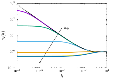
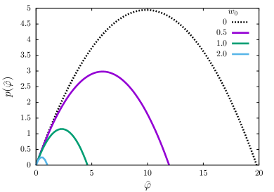
Figure 2: Left: pair distribution function $g_{s}(h)=P(h)$ vs $h$ in the steady state for $w_{0}=0$ (purely repulsive case, black dashed line) and $w_{0}=10^{-3},10^{-2},\ldots,10^{2}$ (colored lines), Eq. (15). The repulsive case displays the $h^{-1/2}$ divergence, while the attractive $w_{0}>0$ curves have a finite limit at $h=0$; the attractive force monotonically depletes the small $h$ region favoring adhesion at $h=0$, as shown by the delta peak amplitude increasing with $w_{0}$. Right: Pressure vs rescaled density as from Eq. (22), with $\widehat{\zeta}=\widehat{\tau}_{p}=\widehat{v}_{0}=\ell=1$. Its behavior is non-monotonic and the decreasing region $\mathrm{d}p/\mathrm{d}\rho<0$ is a possible signal of motility-induced phase separation. The pressure becomes negative after a threshold value of $\widehat{\varphi}$, signaling the unphysical behavior of the computed result.

III.2 Results from dynamical mean-field theory

III.2.1 Microscopic dynamics and infinite-dimensional limit

The general DMFT of infinite-dimensional particle systems interacting through pair potentials and subject to external drivings has been derived in AMZ19 . Here we address the dynamics of active particles introduced in Eq. (1), considering the case of an active Ornstein-Uhlenbeck self-propulsion detailed therein. The latter is microscopically different from run-and-tumble self-propulsion; nevertheless, we recall that the two active forces are equivalent in the limit of infinite space dimension and persistence time. We choose therefore the Ornstein-Uhlenbeck self-propulsion because of its Gaussianity, consistent with the DMFT derivation in AMZ19 . The dimensional scaling of self-propulsion, friction coefficient and density follows the prescriptions introduced in Sec. II.

The DMFT framework allows one to describe the $N$-body, $d$-dimensional process in Eq. (1) by means of a two-body scalar process; indeed, it is known that when $d\rightarrow\infty$ the two-particle process can be determined self-consistently by analyzing the behavior of the rescaled inter-particle gap, i.e.

$$h(t)=h_{0}+y(t)+\Delta_{r}(t)\approx d\left(\frac{r(t)}{\ell}-1\right),$$ (23)

where $r(t)$ is the relative distance between two reference particles, $y(t)=(d/\ell)\,\hat{\mathbf{r}}_{0}\cdot\left(\mathbf{r}(t)-\mathbf{r}_{0}\right)$ is the rescaled projection of the relative displacement along the initial relative direction, and $\Delta_{r}(t)=(d/\ell^{2})\left\langle|\mathbf{x}(t)-\mathbf{x}_{0}|^{2}\right\rangle$ is the mean-square displacement (MSD) contribution given by the $d-1$ transverse components, which is equivalent to the single-particle MSD in the $d\rightarrow\infty$ limit AMZ19 . The equation of motion for $y(t)$ can be shown to take the following form:

$$\begin{split}&\widehat{\zeta}\dot{y}(t)=-\kappa(t)y(t)+\int_{0}^{t}\!\!\mathrm{d}s\,{\cal M}_{R}(t,s)\,y(s)-\widehat{V}^{\prime}(h_{0}+y(t)+\Delta_{r}(t))+\Xi(t)\ ,\qquad y(0)=0\ ,\\ &\left\langle\Xi(t)\right\rangle=0\ ,\quad\left\langle\Xi(t)\Xi(s)\right\rangle=2\widehat{\zeta}T\,\delta(t-s)+{\cal G}_{C}(t-s)+{\cal M}_{C}(t,s)\ ,\qquad{\cal G}_{C}(t)=\widehat{v}_{0}^{2}e^{-|t|/\tau_{p}}\ .\\ \end{split}$$ (24)

The colored noise $\Xi(t)$ has three contributions: (i) the equilibrium thermal bath at temperature $T$. We will drop this term since we will consider the athermal case $T=0$ in the following, but we include it now for the sake of generality; (ii) the active self-propulsion with stationary time correlations ${\cal G}_{C}(t-s)$, corresponding to active Ornstein-Uhlenbeck particles; (iii) the kernel ${\cal M}_{C}(t,s)$, accounting for the force-force correlation given by pairwise interactions. The term $-\widehat{V}^{\prime}(h(t))$ is the rescaled two-particle interaction force. Finally, DMFT also introduces the instantaneous and retarded response kernels, respectively $\kappa(t)$ and ${\cal M}_{R}(t,s)$, to describe the reaction of the $N$-body system on the two-particle process.
The response and correlation kernels $\kappa(t)$, ${\cal M}_{R}(t,s)$ and ${\cal M}_{C}(t,s)$ need to be determined self-consistently with the definitions

$$\begin{split}\kappa(t)&=\frac{\widehat{\varphi}}{2}\int^{\infty}_{-\infty}\,\mathrm{d}h_{0}\,e^{h_{0}}g_{0}(h_{0})\left\langle\widehat{V}^{\prime\prime}(h(t))+\widehat{V}^{\prime}(h(t))\right\rangle_{h_{0}}\ ,\\ {\cal M}_{C}(t,t^{\prime})&=\frac{\widehat{\varphi}}{2}\int^{\infty}_{-\infty}\mathrm{d}h_{0}\,e^{h_{0}}g_{0}(h_{0})\left\langle\widehat{V}^{\prime}(h(t))\widehat{V}^{\prime}(h(t^{\prime}))\right\rangle_{h_{0}}\ ,\\ {\cal M}_{R}(t,t^{\prime})&=\frac{\widehat{\varphi}}{2}\int^{\infty}_{-\infty}\mathrm{d}h_{0}\,e^{h_{0}}g_{0}(h_{0})\left.\frac{\delta\left\langle\widehat{V}^{\prime}(h(t))\right\rangle_{h_{0},{\cal P}}}{\delta{\cal P}(t^{\prime})}\right|_{{\cal P}=0}\\ &=\frac{\widehat{\varphi}}{2}\int^{\infty}_{-\infty}\mathrm{d}h_{0}\,e^{h_{0}}g_{0}(h_{0})\left\langle\widehat{V}^{\prime\prime}(h(t))H(t,s)\right\rangle_{h_{0}}\ ,\end{split}$$ (25)

where $g_{0}(h_{0})$ is the initial gap distribution function, $\left\langle\ldots\right\rangle_{h_{0}}$ refers to an average over the trajectory realizations conditioned to the initial condition $h(0)=h_{0}$, the perturbation ${{\cal P}(t)}$ acts in the pairwise interaction as ${\widehat{V}^{\prime}(h_{0}+y(t)+\Delta_{r}(t))\rightarrow\widehat{V}^{\prime}(h_{0}+y(t)+\Delta_{r}(t)-{\cal P}(t))}$, and the fluctuating response is defined as $H(t,s)=\delta h(t)/\delta{\cal P}(s)|_{{\cal P}=0}$; its evolution is given by

$$\widehat{\zeta}\frac{\partial}{\partial t}H(t,t^{\prime})=-\kappa(t)H(t,t^{\prime})-\widehat{V}^{\prime\prime}(h(t))\left[H(t,t^{\prime})-\delta(t-t^{\prime})\right]+\int^{t}_{t^{\prime}}\mathrm{d}s\,{\cal M}_{R}(t,s)H(s,t^{\prime})\ .$$ (26)

The system is not yet closed, because of the MSD contribution given by $\Delta_{r}(t)$ in Eq. (24); the latter can be determined through the one-particle dynamical correlation and response defined in AMZ19 as

$${\cal C}(t,t^{\prime})=\frac{d}{N\ell^{2}}\sum_{i=1}^{N}\left\langle\delta\mathbf{x}_{i}(t)\cdot\delta\mathbf{x}_{i}(t^{\prime})\right\rangle\ ,\quad{\cal R}(t,t^{\prime})=\frac{d}{N\ell^{2}}\sum_{i,\mu}\left.\frac{\delta\left\langle\delta x_{i\mu}(t)\right\rangle}{\delta\lambda_{i\mu}(t^{\prime})}\right|_{\bm{\lambda}=0}\ ,$$ (27)

where $\delta\mathbf{x}_{i}(t)=\mathbf{x}_{i}(t)-\mathbf{x}_{i}(0)$ is the relative displacement of particle $i$ with respect to its initial position and where the perturbation $\bm{\lambda}_{i}$ appearing in the definition of the response function ${\cal R}(t,t^{\prime})$ acts at the one-particle level as

$$\zeta\dot{\text{\bf x}}_{i}(t)=\text{\bf f}_{i}(t)-\sum_{j(\neq i)}\bm{\nabla}_{\text{\bf x}_{i}}V(\text{\bf x}_{i}-\text{\bf x}_{j})+\bm{\lambda}_{i}(t)\,.$$ (28)

In the limit of infinite dimension, the correlation and response evolve according to the following dynamics

$$\begin{split}\widehat{\zeta}\frac{\partial}{\partial t}{\cal C}(t,t^{\prime})=&2\widehat{\zeta}T{\cal R}(t^{\prime},t)-\kappa(t){\cal C}(t,t^{\prime})+\int_{0}^{t}\mathrm{d}s\,{\cal M}_{R}(t,s){\cal C}(s,t^{\prime})+\int_{0}^{t^{\prime}}\mathrm{d}s\,\left[{\cal G}_{C}(t-s)+{\cal M}_{C}(t,s)\right]{\cal R}(t^{\prime},s)\ ,\\ \widehat{\zeta}\frac{\partial}{\partial t}{\cal R}(t,t^{\prime})=&\frac{\delta(t-t^{\prime})}{2}-\kappa(t){\cal R}(t,t^{\prime})+\int_{t^{\prime}}^{t}\mathrm{d}s\,{\cal M}_{R}(t,s){\cal R}(s,t^{\prime})\ .\end{split}$$ (29)

By definition, one has $\Delta_{r}(t)={\cal C}(t,t)$, and the dynamical equations are at this stage closed. The evolution equation for the MSD $\Delta(t,t^{\prime})=\frac{d}{\ell^{2}}\left\langle|\mathbf{x}(t)-\mathbf{x}(t^{\prime})|^{2}\right\rangle$ and $\Delta_{r}(t)\equiv\Delta(t,0)$ therefore read

$$\begin{split}\widehat{\zeta}\frac{\partial}{\partial t}\Delta(t,t^{\prime})=&-\kappa(t)\left[\Delta(t,t^{\prime})+\Delta_{r}(t)-\Delta_{r}(t^{\prime})\right]+\int_{0}^{t}\mathrm{d}s\,{\cal M}_{R}(t,s)\left[\Delta_{r}(t)-\Delta_{r}(t^{\prime})+\Delta(s,t^{\prime})-\Delta(s,t)\right]\\ &-4\widehat{\zeta}T\,{\cal R}(t^{\prime},t)+2\int_{0}^{\max(t,t^{\prime})}\mathrm{d}s\,\left[{\cal G}_{C}(t-s)+{\cal M}_{C}(t,s)\right]\left[{\cal R}(t,s)-{\cal R}(t^{\prime},s)\right]\ ,\\ \widehat{\zeta}\dot{\Delta}_{r}(t)=&-2\kappa(t)\Delta_{r}(t)+\int_{0}^{t}\mathrm{d}s\,{\cal M}_{R}(t,s)\left[\Delta_{r}(t)+\Delta_{r}(s)-\Delta(s,t)\right]+2\int_{0}^{t}\mathrm{d}s\,\left[{\cal G}_{C}(t-s)+{\cal M}_{C}(t,s)\right]{\cal R}(t,s)\ .\end{split}$$ (30)

We stress that, in this framework, the solution of the dynamics is not stationary nor time-translationally invariant and depend on the initial condition, i.e. the choice of the initial distribution $g_{0}(h_{0})$. The solution of the DMFT equations therefore yields the transient dynamics at short times and the eventual steady-state dynamics at long times.

III.2.2 Dilute solution with infinite persistence

The analytical solution of the problem determined by Eqs. (24-29) is currently out of reach. In the equilibrium case, these equations simplify thanks to fluctuation-dissipation relations and a numerical solution has been found MSZ20 . In the present case, a numerical solution must deal with strong technical difficulties, the main one being the sampling efficiency at long times: indeed, particles with infinite persistence time eventually collide with a rate that is exponentially decaying in time. Therefore, the amount of trajectories needed to compute the dynamical kernels at long time is exponentially high. A possible solution may involve the generation of biased trajectories to increase efficiency, but its design goes beyond the scope of this article.

It is however possible to derive an analytical solution in the dilute limit: indeed, the implicit equations (25) for the kernels depend on the density only through a global multiplicative coefficient. Therefore, a solution for e.g. the instantaneous response $\kappa(t)$ reads

$$\kappa(t)=\widehat{\varphi}\,{\cal F}\left[\kappa,{\cal M}_{R},{\cal M}_{C}\right](t)\ .$$ (31)

An iterative solution can be found assuming that the low-density limit is continuous and that the series

$$\kappa(t)=\widehat{\varphi}\,\kappa^{(1)}(t)+\widehat{\varphi}^{2}\kappa^{(2)}(t)+\ldots\ .$$ (32)

converges. An iterative solution therefore starts with a guess on the initial kernels $\kappa(t),\>{\cal M}_{R}(t,t^{\prime})$ and ${\cal M}_{C}(t,t^{\prime})$; after solving the stochastic dynamics in Eqs. (24,26) with fixed kernels, the latter are updated through Eq. (25). The self-consistent kernels are given by the fixed points of Eq. (31).

When $\widehat{\varphi}=0$, the kernels are trivially vanishing because no interaction occurs. In the dilute limit $\widehat{\varphi}\ll 1$, the solution can be approximated by the first-order expansion in Eq. (32). The latter can be analytically computed in the infinite persistence time limit $\tau_{p}\rightarrow\infty$: indeed, in that case the active force reduces to a constant driving and, in absence of dynamical kernels, the trajectories in Eq. (24) are fully determined by the self-propulsion $\Xi(t)\equiv\Xi_{0}$ drawn at $t=0$.

The solution of the fluctuating equations (24) and (26) can be then computed imposing $\kappa(t)={\cal M}_{R}(t,t^{\prime})={\cal M}_{C}(t,t^{\prime})=0$ and plugging the trajectories $h(t)$ into Eqs. (25) to compute the first-order kernels.

III.2.3 Analytical solution in the dilute limit: trajectories and pair distribution function

In the case of vanishing kernels and at $T=0$, the response and correlation read

$$\begin{split}{\cal R}(t,t^{\prime})&=\frac{1}{2\widehat{\zeta}}\,\theta(t-t^{\prime})\ ,\\ {\cal C}(t,t^{\prime})&=\frac{\widehat{v}_{0}^{2}}{2\widehat{\zeta}^{2}}\,t\,t^{\prime}\quad\Rightarrow\quad\Delta(t,t^{\prime})=\frac{\widehat{v}_{0}^{2}}{2\widehat{\zeta}^{2}}(t-t^{\prime})^{2}\ .\end{split}$$ (33)

This solution is nothing but the dynamics of a single free active particle moving across a medium with rescaled friction coefficient $\widehat{\zeta}$, rescaled self-propulsion $\widehat{v}_{0}$ and infinite persistence time $\tau_{p}$. Indeed the response is a step function, i.e. a perturbation of the position at time $t^{\prime}$ remains unchanged at any $t>t^{\prime}$, and the MSD makes clear that the particle moves ballistically with effective speed $\widehat{v}_{0}/\widehat{\zeta}$. This result represents the first step towards a two-particle solution, and depends on a natural time scale $\tau_{0}=\widehat{\zeta}/\widehat{v}_{0}$, which represents the typical duration of a collision, as it is the time needed to traverse a distance $\ell/d$ at speed $v_{0}$. This time scale must not be confused with $\tau_{p}$, which we recall to be the persistence time of the active self-propulsion. In the following, we will set $\widehat{\zeta}=\widehat{v}_{0}=1$, setting $\tau_{0}$ as unit of time and $\widehat{v}_{0}$ as unit of energy; the dimensional coefficients will be reinstated in the final results. The solution in Eq. (33) leads to the dynamical equation for $h(t)=h_{0}+y(t)+\Delta_{r}(t)$

$$\begin{gathered}\dot{h}(t)=-\widehat{V}^{\prime}(h(t))+\xi_{0}+t\ ,\quad h(0)=h_{0}\\ \left\langle\xi_{0}\right\rangle=0\ ,\quad\langle\xi_{0}^{2}\rangle=1\ ,\end{gathered}$$ (34)

having now called $\Xi(t)=\Xi_{0}=\widehat{v}_{0}\,\xi_{0}$. The equation for the fluctuating response $H(t,t^{\prime})$ now reads

$$\frac{\partial}{\partial t}H(t,t^{\prime})=-\widehat{V}^{\prime\prime}(h(t))\left[H(t,t^{\prime})-\delta(t-t^{\prime})\right]\ .$$ (35)

The last equations must be solved with an appropriate choice of the potential. We consider a sticky-sphere potential as defined in Eq. (9), always taking $\widehat{v}_{0}=1$, and will study the dynamics in the same limit with $\lambda\rightarrow\infty$ corresponding to a hard core and an infinitely narrow attractive region, with a constant adhesive force when $h=0$.

Our goal is to compute the pair distribution function and the dynamical kernels based on the dynamical equations above. The first one is given by AMZ19

$$g(h,t)=e^{-h}\int\mathrm{d}h_{0}\,g_{0}(h_{0})\,e^{h_{0}}\left\langle\delta(h(t)-h)\right\rangle_{h_{0}}\ .$$ (36)

In our settings, this average is equivalent to the average over the unitary normal variable $\xi_{0}$. The pair distribution evolution depends on the initial distribution $g_{0}(h_{0})$; however, the steady state limit must not depend on its choice, so we choose to work with $g_{0}(h_{0})=\theta(h_{0}-1/\lambda)$, so that the particles are not interacting at the initial time.

Given these premises, the pair distribution function can be directly computed in the hard-sphere limit. Indeed, when $\lambda\rightarrow\infty$, the particles are unable to overlap at $h<0$, and feel a finite attractive force with strength $w_{0}$ when $h=0$. The trajectories can be then divided into external and colliding ones. The former simply follow a ballistic motion with initial velocity $\xi_{0}$ and unitary acceleration; the latter are divided in three zones: (i) a ballistic motion for $t<t_{1}$, being $t_{1}$ the starting time of the collision; (ii) the sticky collision, i.e. $h(t)=0$ for $t_{1}<t<t_{2}$, being $t_{2}$ the time when the particle leaves the barrier; (iii) a ballistic motion for $t>t_{2}$. Namely,

$$h(t)=h_{0}+\xi_{0}\,t+\frac{1}{2}t^{2}\qquad\text{for external trajectories,}$$ (37)

and

$$h(t)=\begin{cases}h_{0}+\xi_{0}\,t+\frac{1}{2}t^{2}&t<t_{1}=-\xi_{0}-\sqrt{\xi^{2}_{0}-2h_{0}}\\ 0&t_{1}<t<t_{2}=-\xi_{0}+w_{0}\\ \frac{1}{2}\left[(t+\xi_{0})^{2}-w_{0}^{2}\right]&t>t_{2}\end{cases}\qquad\text{for colliding trajectories.}$$ (38)

At any time $t$, $h(t)$ is determined by the values of $\xi_{0}$ and $h_{0}$; the trajectories at contact with the barrier will contribute to the delta peak in $h=0$, while the trajectories with $h>0$ will give the regular part of the pair distribution function. Injecting the solution above into the equation for $g(h,t)$ one has the time-dependent solution

$$\begin{split}g(h,t)&=G(t)\,\delta(h)+g_{r}(h,t)\ ,\\ G(t)&=\begin{cases}\frac{t}{\sqrt{2\pi}}\quad&\text{for }t<w_{0}\\ \frac{1}{2}+\frac{w_{0}}{\sqrt{2\pi}}-\frac{1}{2}\mathrm{erfc}\frac{t-w_{0}}{\sqrt{2}}\quad&\text{for }t>w_{0}\end{cases}\ ,\\ g_{r}(h,t)&=\begin{cases}\frac{1}{2}\left(1+\mathrm{erf}\sqrt{h}\right)+\frac{e^{-h}}{\sqrt{2\pi(2h+w_{0}^{2})}}\left[1-e^{-\frac{1}{2}\left(t-\sqrt{2h+w_{0}^{2}}\right)^{2}}\right]&\text{for }0<h<\frac{t^{2}-w_{0}^{2}}{2}\ ,\\ \frac{1}{2}\left(1+\mathrm{erf}\sqrt{h}\right)&\text{for }\frac{t^{2}-w_{0}^{2}}{2}<h<\frac{t^{2}}{2}\ ,\\ \frac{1}{2}\left[1+\mathrm{erf}\left(\frac{2h+t^{2}}{2\sqrt{2}\,t}\right)\right]&\text{for }h>\frac{t^{2}}{2}\ ,\\ \end{cases}\end{split}$$ (39)

leading to the steady state limit for $t\rightarrow\infty$:

$$g_{s}(h)=\Theta(h)\left[\frac{1}{2}\left(1+\mathrm{erf}\sqrt{h}\right)+\frac{e^{-h}}{\sqrt{2\pi(2h+w_{0}^{2})}}\right]+\left(\frac{1}{2}+\frac{w_{0}}{\sqrt{2\pi}}\right)\delta(h)\ .$$ (40)

This result is equivalent to Eq. (15) in the steady state, and adds new information on the transient behavior of the pair distribution function. In particular, the delta peak emerges continuously with time and has a singular behavior at $t=w_{0}$. When $w_{0}=0$, we fall back on the purely repulsive hard-sphere potential studied in Ref. ALW19 .

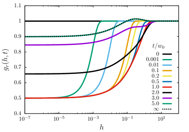
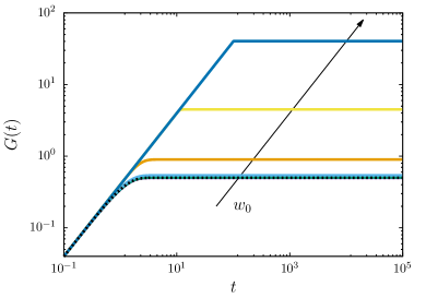
Figure 3: Left: the regular part of the pair distribution function $g_{r}(h,t)$ vs $h$ at several times (see key), given by Eq. (39) with $w_{0}=1$. The small-gap region $h\ll 1$ is rapidly depleted by means of adhesive collisions. When $t>w_{0}$, the self-propulsion overcomes the attractive force, the particles leave the adhesive boundary and the small $h$ region becomes populated again. Right: the delta peak amplitude $G(t)$ vs $t$ for $w_{0}=0$ (purely repulsive case, black dashed line) and $w_{0}=10^{-3},10^{-2},\ldots,10^{2}$ (colored lines). The linear growth at short times is followed by a steady state at longer times, where $G(t)\rightarrow 1/2+w_{0}/\sqrt{2\pi}$.

III.2.4 Dynamical kernels

The computation of dynamical kernels requires the evaluation of the potential and its derivatives, and thus cannot be performed in the hard limit $\lambda\rightarrow\infty$, since in that case all these terms are singular. We then need to solve the equations of motion for the regular potential in Eq. (9). Those can be solved by parts for three interaction scenarios: (i) the external case $h(t)>1/\lambda$ for all $t$, (ii) the colliding case $h(t)<0$ at some $t$ and (iii) an intermediate, tangential case for which there exists $h(t)<1/\lambda$ but $h(t)>0$ at any $t$, which means that the particles enter the mutual attraction region but never get to the repulsive core. This case disappears in the hard potential limit, where the width of the attractive region vanishes, but must be nevertheless accounted for in the course of the kernel computation.

The details of the computation are reported in Appendix B.1. As can be foreseen from Eqs. (25) the response kernels $\kappa(t)$ and ${\cal M}_{R}(t,s)$ are divergent in the hard-sphere limit; however, their divergences compensate in that limit, as shown in Appendix B.3. We also argue that in the hard-sphere limit the repulsive interactions give rise to a short-ranged memory kernel ${\cal M}_{R}(t,s)$: as shown in Appendix B.2, the fluctuating response vanishes over a time scale proportional to $\lambda^{-1}$ and therefore only the near past of a dynamical variable contributes to the response term. The integrated response can be then expanded as

$$\begin{split}\int_{0}^{t}\mathrm{d}s\,{\cal M}_{R}(t,s)\,f(s)&=\int_{0}^{t}\mathrm{d}s\,{\cal M}_{R}(t,s)\left[f(t)-\dot{f}(t)(t-s)+\frac{1}{2}\ddot{f}(t)(t-s)^{2}+\ldots\right]\\ &=\chi_{0}(t)\,f(t)-\chi_{1}(t)\,\dot{f}(t)+\frac{1}{2}\chi_{2}(t)\,\ddot{f}(t)+\ldots\ ,\end{split}$$ (41)

being $f(s)$ is a continuous function of time. The latter equation is nothing but a Taylor expansion of the function $f(s)$ in the integral for $s\approx t^{-}$, assuming that the response kernel ${\cal M}_{R}(t,s)$ is peaked at $s=t$ and rapidly decaying over time. The integrated response moments $\chi_{n}(t)$ are defined as

$$\chi_{n}(t)\equiv\int^{t}_{0}\mathrm{d}s\,{\cal M}_{R}(t,s)\,(t-s)^{n}\ .$$ (42)

It is shown in Appendix B.4 that the moments with $n\geq 2$ vanish in the hard-sphere limit. Using this property, the general motion equation (24) for $y(t)$ can be approximated for $\lambda\gg 1$ as

$$\widehat{\zeta}\dot{y}(t)=-\gamma(t)\,y(t)-\chi_{1}(t)\,\dot{y}(t)-\widehat{V}^{\prime}(h(t))+\Xi(t)\ ,$$ (43)

where $\gamma(t)\equiv\kappa(t)-\chi_{0}(t)$, and the same transformation can be applied to all the dynamical equations containing the two reaction terms $\kappa(t)$ and ${\cal M}_{R}(t,s)$. Their physical meaning is transparent: the first coefficient $\gamma(t)$ is an elastic coefficient and we expect it to vanish in the long-time limit, since we are in the dilute phase and the individual trajectories are not dynamically arrested near their initial position. The second coefficient gives the first-order density correction to the bare friction coefficient $\widehat{\zeta}$, the main information needed to understand how a small density affects the dynamics. We also underline that this expansion does not depend on the low density assumption but on the hard-sphere interactions, and holds at any density.

The computation of the dynamical kernels is tedious and mostly technical, and is therefore deferred to Appendix B.3. It relies on the computation of the two-particle process $h(t)$ and on the fluctuating response $H(t,s)$, which are respectively performed in Appendix B.1 and B.2. Altogether, in the long-time limit one gets

$$\gamma_{\infty}=0\ ,\quad\chi^{\infty}_{1}=\frac{\widehat{\varphi}}{4}\widehat{\zeta}\,\left(1+\frac{\sqrt{2}}{3\sqrt{\pi}}w_{0}^{3}\right)\equiv\frac{\widehat{\varphi}}{\widehat{\varphi}_{0}(w_{0})}\,\widehat{\zeta}\ .$$ (44)

III.2.5 Effective propulsion

The last result allows us to compute the effective propulsion in the steady state, namely the velocity along the self-propulsion direction. To do so, we write the equation for the displacement of a generic particle $\delta\mathbf{x}(t)=\mathbf{x}(t)-\mathbf{x}_{0}$, derived through a dynamical cavity method Sz17 , before the infinite-dimensional rescaling AMZ19 . This reads

$$\begin{gathered}\zeta\dot{\delta\mathbf{x}}(t)=-k(t)\delta\mathbf{x}(t)+\int_{0}^{t}\mathrm{d}sM_{R}(t,s)\delta\mathbf{x}(s)+\text{\bf f}(t)+\bm{\xi}(t)\ ,\\ \left\langle f_{\mu}(t)\right\rangle=0\ ,\quad\left\langle f_{\mu}(t)f_{\nu}(t^{\prime})\right\rangle=\delta_{\mu\nu}\,\Gamma_{C}(t-t^{\prime})\ ,\\ \left\langle\xi_{\mu}(t)\right\rangle=0\ ,\quad\left\langle\xi_{\mu}(t)\xi_{\nu}(t^{\prime})\right\rangle=\delta_{\mu\nu}\left[2\zeta\,T\,\delta(t-t^{\prime})+M_{C}(t,t^{\prime})\right]\ ,\end{gathered}$$ (45)

where we included a white thermal noise in the dynamics for the sake of generality, that we will eventually drop in the following setting $T=0$ as usual. We then define the dynamical observable $A(t,t^{\prime})$

$$A(t,t^{\prime})=\frac{\zeta}{v_{0}}\left\langle\delta\mathbf{x}(t)\cdot\text{\bf f}(t^{\prime})\right\rangle\ ,$$ (46)

measuring the total displacement at time $t$ along the direction of the active force at time $t^{\prime}$. This quantity leads to the definition of the effective propulsion $v(\widehat{\varphi})$ as

$$v(\widehat{\varphi})=\left.\frac{\partial}{\partial t}A(t,t^{\prime})\right|_{t=t^{\prime}}=\frac{1}{v_{0}}\left\langle\zeta\dot{\delta\mathbf{x}}(t)\cdot\text{\bf f}(t)\right\rangle\ ,$$ (47)

which is a time-translationally invariant observable in the steady state. So, at zero density, the free-particle is moving at the bare self-propulsion speed $v_{0}$, and we expect $v(\widehat{\varphi})$ to decrease monotonically with the density.

The quantity $A(t,t^{\prime})$ follows the dynamical equation

$$\partial_{t}A(t,t^{\prime})=-k(t)A(t,t^{\prime})+\int_{0}^{t}\mathrm{d}s\,M_{R}(t,s)A(s,t^{\prime})+\frac{d\zeta}{v_{0}}\Gamma_{C}(t-t^{\prime})\ ,$$ (48)

having exploited the independence between the active noise and the fluctuations of the inter-particle interactions, i.e. $\left\langle\bm{\xi}(t)\cdot\text{\bf f}(t^{\prime})\right\rangle=0$.

When $t,t^{\prime}\rightarrow\infty$, we obtain the steady-state dynamical equation

$$\zeta\partial_{t}A(t,t^{\prime})=-g(t)A(t,t^{\prime})-c_{1}(t)\partial_{t}A(t,t^{\prime})+\frac{d\zeta}{v_{0}}\Gamma_{C}(t-t^{\prime})\ ,$$ (49)

where $g(t)=k(t)-\int^{t}_{0}\mathrm{d}s\,M_{R}(t,s)=(2d^{2}/\ell^{2})\gamma(t)\rightarrow 0$ and $c_{1}(t)=\int^{t}_{0}\mathrm{d}s\,M_{R}(t,s)\,(t-s)=(2d^{2}/\ell^{2})\chi_{1}(t)\rightarrow c^{\infty}_{1}$ when $t\rightarrow\infty$. The last results hold for $\Gamma_{C}(t-t^{\prime})=v_{0}^{2}/d$, and the total friction coefficient reads $\zeta+c_{1}^{\infty}=\zeta(1+\widehat{\varphi}/\widehat{\varphi}_{0})$. Their derivation is presented in Sec. B.3, and is given by the computation of the first two integrated response moments in the limit of dilute hard spheres. So, Eq. (47) gives us

$$v(\widehat{\varphi})=\frac{v_{0}}{1+\widehat{\varphi}/\widehat{\varphi}_{0}(w_{0})}\ .$$ (50)

This is the fundamental result of this calculation. We show then that, to the first order in $\widehat{\varphi}$, the effective propulsion in a dilute media is damped by a factor $1+\widehat{\varphi}/\widehat{\varphi}_{0}(w_{0})$, accounting for the slowing down of particles’ velocity caused by interactions. Considering the dilute limit approximation $\widehat{\varphi}\ll 1$, its first-order expansion in $\widehat{\varphi}$ coincides with the result obtained from Fokker-Planck equation in Eq. (18).

It is worth noticing that the last result can be generalized to relate the friction coefficient and the effective self-propulsion with the steady-state pair distribution function. Indeed from Eq. (42) one also has

$$\chi^{\infty}_{1}=\frac{\widehat{\varphi}}{2}\int^{+\infty}_{-\infty}\mathrm{d}h\,e^{h}g_{s}(h){\cal K}^{\infty}(h)\ ,\quad{\cal K}(h,t)=\int_{0}^{t}\mathrm{d}s\,(t-s)\left\langle\widehat{V}^{\prime\prime}(h(t))H(t,s)\right\rangle_{h}\ ,$$ (51)

being ${\cal K}^{\infty}(h)=\lim_{t\rightarrow\infty}{\cal K}(h,t)$.

IV Transient behavior of Hard Spheres

When $w_{0}=0$, we recover the purely repulsive hard-sphere interaction potential, namely

$$\widehat{V}_{\rm HS}(h)=\begin{cases}\infty&h<0\\ 0&h>0\end{cases}\ .$$ (52)

All calculations above are valid for the case $w_{0}=0$. Furthermore, in this case one can also compute the transient dynamics of the dynamical kernels defined in Eqs. (25), which were analytically unattainable in the general sticky spheres case. With the same procedure as in the previous section, we approximate the hard-sphere potential with a soft-sphere one, namely $\widehat{V}(h)=\dfrac{\varepsilon}{2}h^{2}\theta(-h)$. The hard-sphere potential is recovered in the $\varepsilon\rightarrow\infty$ limit. This soft-sphere potential is equivalent to the sticky-sphere one defined in Eq. (9), in the limit $w_{0}\rightarrow 0$ and $\lambda\rightarrow\infty$ keeping $\lambda w_{0}=\varepsilon$ fixed, and it is the same interaction potential already analyzed in the solution of equilibrium dynamics presented in MSZ20 .

This choice makes the analytical computation of the dynamical kernels much easier; indeed, one can follow the same scheme described for sticky spheres to access the pair distribution function $g(h,t)$ and the dynamical kernels $\kappa(t)$, ${\cal M}_{R}(t,s)$ and ${\cal M}_{C}(t,s)$. The time evolution of the pair distribution function is given by Eq. (39), setting $w_{0}=0$. For the dynamical kernels, we can avoid the limit $t\rightarrow\infty$ in their calculation; we get then the first integrated response moments, finally leading to

$$\begin{split}\gamma(t)&=\frac{\widehat{\varphi}}{2}\widehat{v}_{0}\,\left[\frac{e^{-t^{2}/2}}{\sqrt{2\pi}}-\frac{t}{2}\,\mathrm{erfc}\left(\frac{t}{\sqrt{2}}\right)\right]\ ,\\ \chi_{1}(t)&=\frac{\widehat{\varphi}}{4}\widehat{\zeta}\,\mathrm{erf}\left(\frac{t}{\sqrt{2}}\right)\ ,\\ {\cal M}_{C}(t,s)&=\frac{\widehat{\varphi}}{4}\widehat{v}_{0}^{2}\,\left[\mathrm{erfc}\left(\frac{|t-s|}{\sqrt{2}}\right)+\mathrm{erfc}\left(\frac{t}{\sqrt{2}}\right)(1+ts)-\sqrt{\frac{2}{\pi}}s\,e^{-t^{2}/2}\right]\ ,\end{split}$$ (53)

always expressing the time $t$ in units of the natural time scale $\tau_{0}=\widehat{\zeta}/\widehat{v}_{0}$. The steady-state limit is the same as that described for the sticky-sphere case, i.e. $\gamma_{\infty}=0$ and $\chi^{\infty}_{1}=\dfrac{\widehat{\varphi}}{4}\,\widehat{\zeta}\equiv\dfrac{\widehat{\varphi}}{\widehat{\varphi}_{0}}\,\widehat{\zeta}$. Furthermore, we can characterize the noise correlation in the long-time limit, where the noise only depends on the time difference $\tau=t-s$, namely

$${\cal M}^{\infty}_{C}(\tau)=\frac{\widehat{\varphi}}{4}\widehat{v}_{0}^{2}\,\mathrm{erfc}\frac{|\tau|}{\sqrt{2}}\ .$$ (54)

The above result allows us to derive the behavior of the MSD in the long-time limit; indeed, with the kernels computed in Eq. (53), the correlation-response equations now read

$$\begin{split}\widehat{\zeta}\frac{\partial}{\partial t}{\cal R}(t,t^{\prime})&=\frac{\delta(t-t^{\prime})}{2}-\gamma(t){\cal R}(t,t^{\prime})-\chi_{1}(t)\frac{\partial}{\partial t}{\cal R}(t,t^{\prime})\ ,\\ \widehat{\zeta}\frac{\partial}{\partial t}{\cal C}(t,t^{\prime})&=-\gamma(t){\cal C}(t,t^{\prime})-\chi_{1}(t)\frac{\partial}{\partial t}{\cal C}(t,t^{\prime})+\int^{t^{\prime}}_{0}\mathrm{d}s\,\left[{\cal G}_{C}(t-s)+{\cal M}_{C}(t,s)\right]{\cal R}(t^{\prime},s)\ .\end{split}$$ (55)

The first equation can be explicitly solved in the steady-state limit, giving

$${\cal R}^{\infty}(\tau)=\frac{1}{2\widehat{\zeta}(1+\widehat{\varphi}/\widehat{\varphi}_{0})}\theta(\tau)\ .$$ (56)

With this result, from Eq. (30) one can derive an equation for the MSD in the steady-state limit $t,t^{\prime}\gg 1$, as a function of the dimensionless time difference $\tau=t-t^{\prime}$, i.e.

$$\dot{\Delta}^{\infty}(\tau)=\frac{1}{(1+\widehat{\varphi}/\widehat{\varphi}_{0})^{2}}\left\{\tau+\frac{\widehat{\varphi}}{\widehat{\varphi}_{0}}\left[\tau\,\mathrm{erfc}\frac{\tau}{\sqrt{2}}+\sqrt{\frac{2}{\pi}}\left(1-e^{-\tau^{2}/2}\right)\right]\right\}\ ,$$ (57)

and this equation can be easily integrated, yielding

$$\Delta^{\infty}(\tau)=\frac{1}{(1+\widehat{\varphi}/\widehat{\varphi}_{0})^{2}}\left\{\frac{\tau^{2}}{2}+\frac{\widehat{\varphi}}{\widehat{\varphi}_{0}}\left[\frac{\tau}{\sqrt{2\pi}}\left(2-e^{-\tau^{2}/2}\right)-\frac{1}{2}\mathrm{erf}\frac{\tau}{\sqrt{2}}+\frac{\tau^{2}}{2}\mathrm{erfc}\frac{\tau}{\sqrt{2}}\right]\right\}\ .$$ (58)

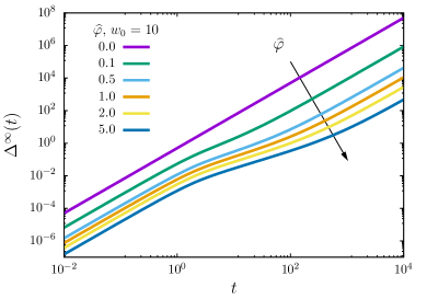
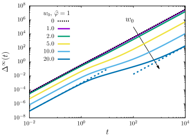
Figure 4: Steady-state mean squared displacement $\Delta^{\infty}(t)$ vs $t$ from Eq. (58) for several values of rescaled density $\widehat{\varphi}$ (left, $w_{0}=10$) and attractive force $w_{0}$ (right, $\widehat{\varphi}=1$). The MSD is ballistic at short and long times, but the increase in density or in adhesion induces a slowdown at intermediate times, respectively given by the many-body interactions or the duration of an adhesive collision. We compare the short and long time behavior from Eq. (59) for the case $w_{0}=20$ in the right panel (dashed blue lines).

The solution above shows that the dynamics is ballistic at short and long times, with a slowdown at intermediate times given by the presence of interactions. With the effective propulsion definition computed in Eq. (50), it is clear that

$$\Delta^{\infty}(\tau)\sim\frac{v(\widehat{\varphi})^{2}}{2\widehat{\zeta}^{2}}\tau^{2}\times\begin{cases}1+\widehat{\varphi}/\widehat{\varphi}_{0}&\tau\ll\tau_{0}\\ 1&\tau\gg\tau_{0}\end{cases}$$ (59)

with $\tau_{0}=\widehat{\zeta}/\widehat{v}_{0}$. The last result can be interpreted in the following way: at any time, the interplay between self-propulsion and pairwise interactions yields an effective self-propulsion $v(\widehat{\varphi})$ for the single particle, hence the common prefactor in the rhs of Eq. (59). At short times, however, the fluctuations of pairwise interactions $\bm{\xi}(t)$ are correlated and therefore contribute to the MSD with an additional term as shown above. At longer times, conversely, the fluctuations always decorrelate in the dilute phase and the dominant contribution to the MSD is given by the effective self-propulsion.

V Conclusions

In this paper, we implemented two alternative approaches to investigate the dynamics of active particles embedded in a large-dimensional space. The results from kinetic theory, previously presented in ALW19 , have been extended to the case of a non-monotonous potential featuring an attractive component, and compared with the results of dynamical mean-field theory in the low-density limit and at large persistence time. The two methods have been proven to be consistent in the steady-state limit within this frameword; indeed, the calculation of the pair distribution function has given the same result in both cases, and we added a more detailed description in term of the rescaled inter-particle gap $h(t)$, which is the physically interesting variable in the high-dimensional limit. Finally, we have explicitly computed the effect of an infinitely short-ranged attractive potential on the amplitude of the adhesive delta peak in $g(h)$.

Furthermore, we also computed the effective propulsion $v(\widehat{\varphi})$ of the active particles, namely the effective velocity at which particles are propelled once the effect of the interactions have been considered. Again, the two approaches converged to the same results, taking into account that this result is obtained in the dilute limit. The extrapolation of the effective self-propulsion to higher densities can lead to interpret $\widehat{\varphi}_{0}(w_{0})$ as the crowding density, i.e. the value of the density at which the active particles get stuck in an arrested phase with no room to move any longer ALW19 . We remark that for purely repulsive hard spheres one has $\widehat{\varphi}_{0}=4$, and this value decreases when adhesion is present. On the other hand, it is known parisi2020theory that hard spheres in equilibrium undergo a dynamical glass transition at $\widehat{\varphi}=\widehat{\varphi}_{d}\simeq 4.8067$, where the mean square displacement converges to a finite but positive limit; conversely, both the effective propulsion and the mean square displacement vanish in the crowded phase. We stress that the result for the crowding density is however extrapolated from the dilute phase, and that it must be taken as a first step towards a solution in the dense phase, where the crowding and glass transitions can be compared properly.

The last part of our analysis has been dedicated to the transient behavior of hard spheres by means of dynamical mean-field theory; it has been shown how, starting from an equilibrium configuration, the system relaxes towards a stationary state. This relaxation is described by the transient part of the dynamical coefficients, and in this limit we computed the MSD in the steady state, elucidating how the interplay between active self-propulsion and interactions affects its short-time behavior, while the infinitely persistent self-propulsion dominates at long times.

These results constitute a starting point for a more complete analysis of active systems in high dimensions. The next step along this line of research is its extension to higher densities and finite persistence times. This task being severely hard to accomplish via analytical tools, a numerical solution of DMFT equations must be found, in line with previous results RBBC19 ; MSZ20 . However, if the self-propulsion is too strong or too persistent, the trajectories drift away and the solution relies on the statistics of exponentially rare events. The development of importance-based algorithms is then required and would give an important edge in the solution of the problem at any density.

Another approach that may be tackled in the future concerns the limit of small persistence time; in that case, often studied in active matter systems FNCTVvW16prl ; FS20pre the dynamics can be perturbatively studied starting from the equilibrium solution. Its analysis would lead to understand how a small amount of activity affects the dynamics, i.e. the behavior of dynamical kernels, the interplay between the dynamical transition and the crowding transition, and the effects on fluctuation-dissipation relations.

Data Availability

Data sharing is not applicable to this article as no new data were created or analyzed in this study.

Appendix A Solving the two-body Fokker-Planck equation

In this Appendix, we solve Eq. (8) using the method of characteristics for the sticky-sphere potential. We start by establishing Eq. (11) and Eq. (12) of the main text which describe the $\lambda\rightarrow\infty$ limit of the stationary distribution. For $h>1/\lambda$, we obtain first

$$w\,\partial_{h}P+\partial_{w}P=0\,.$$ (60)

In the limit $\lambda\rightarrow\infty$, we thus recover Eq. (11) of the main text. Next, for $h<1/\lambda$ and for any function $j(h)$ independent of $\lambda$ we define

$$\Gamma^{\lambda}_{j}(w)=\int_{-\infty}^{1/\lambda}\text{d}h\,e^{h}P(h,w)j(h)\,,$$ (61)

so that Eq. (8) yields

$$-\widehat{v}_{0}\partial_{w}\Gamma^{\lambda}_{j}(w)+\widehat{v}_{0}w\Gamma^{\lambda}_{j}(w)-\widehat{v}_{0}w\left(P\left(1/\lambda,w\right)j\left(1/\lambda\right)e^{1/\lambda}\right)+\widehat{v}_{0}w\Gamma^{\lambda}_{j^{\prime}}(w)-\int_{-\infty}^{1/\lambda}\text{d}h\,e^{h}\frac{\widehat{V}^{\prime}(h)}{\ell}j^{\prime}(h)P(h,w)=0\,.$$ (62)

In the limit $\lambda\rightarrow\infty$, the stationary distribution function decays to $0$ as $h<0$ over scales $O(1/\lambda)$ and we have

$$\Gamma^{\lambda}_{j}(w)\xrightarrow[\lambda\rightarrow\infty]{}j(0)\lim_{\lambda\rightarrow\infty}\int_{-\infty}^{1}\frac{\text{d}h}{\lambda}\,e^{h/\lambda}\,P\left(\frac{h}{\lambda},\,w\right)=f(0)\,\Gamma(w)\,,$$ (63)

provided the previous limit exists. This justifies the functional form in Eq. (10) of the main text. Hence, on one hand, for a function $j$ defined such that $j^{\prime}(0)=0$, Eq. (62) yields Eq. (12)

$$\Gamma^{\prime}(w)-w\Gamma(w)=-w\lim_{\lambda\rightarrow\infty}P\left(1/\lambda,w\right)\,.$$ (64)

On the other hand, for a function $j$ such that $j(0)=0$, Eq. (62) yields the integrated version of Eq. (19)

$$\lim_{\lambda\rightarrow\infty}\int_{-\infty}^{1/\lambda}\text{d}h\,e^{h}j^{\prime}(h)\frac{\widehat{V}^{\prime}(h)}{l}P(h,w)=\widehat{v}_{0}wj^{\prime}(0)\Gamma(w)\ ,$$ (65)

which gives the limit of the product $\widehat{V}^{\prime}(h)P(h,w)$ as $\lambda\rightarrow\infty$. Eventually, since $\widehat{V}^{\prime}(h)<\widehat{v}_{0}w_{0}$, we obtain from Eq. (65)

$$\Gamma(w)\left(w-w_{0}\right)\leq 0\,,$$ (66)

which, given the positivity of $\Gamma(w)$, yields

$$\Gamma(w>w_{0})=0\,.$$ (67)

We are now in position to solve Eq. (11) and Eq. (12). In Sec. III.2.3, the same stationary distribution will be derived in an alternative way directly from the equations of motion. For $h>0$, Eq. (11) tells us that $P^{b}(h,w)$ is constant along the characteristics $2h-w^{2}=\text{cst}$ that correspond to deterministic trajectories. These characteristic lines are depicted in Fig. 5. We solve the equations with the boundary condition

$$P^{b}(L,x<0)=1\,,$$ (68)

where $L$ is some large length scale introduced to treat the boundary conditions that will eventually be sent to infinity. In the relative-particle-around-a-spherical-obstacle picture this corresponds to a homogeneous reservoir of incoming particles at $h=L$. As $L$ is sent to infinity this expresses the isotropy of the stationary distribution at large distances.

\begin{overpic}[totalheight=170.71652pt]{characteristics.jpg} \put(72.0,3.0){$w_{0}$} \put(50.65,3.0){$0$} \put(52.0,36.5){$L$} \end{overpic}

Figure 5: Characteristics in the ($w,h$) plane.

The blue domain in Fig. 5, i.e. $\{w<0,h\}\cup\{w>0,2h-w^{2}>0\}$, is made of characteristics that intersect the boundary half line $\{x<0,h=L\}$. The quantity $P^{b}$ is thus constant and equal to one in this domain. On the contrary, $P^{b}$ vanishes in the orange ($\{w>0,0>2h-w^{2}>-w_{0}^{2}\}$) and green ($\{w>0,2h-w^{2}<-w_{0}^{2}\}$) ones. Indeed, we have first $\Gamma(w>w_{0})=0$ so that Eq. (12) implies $P^{b}(0,w>w_{0})=0$ and the vanishing of $P^{b}$ in the green domain. Then, we notice that the orange domain corresponds to trajectories in which the two particles escape from a collision event with $0<w<w_{0}$. However, given the shape of the potential in Eq. (9), this never happens. Eventually, the red line $2h-w^{2}=-w_{0}^{2}$ in Fig. 5 plays a special role. Indeed, all trajectories leading to a collision event between the two particles collapse onto this line as they separate afterwards. We thus look for a solution of Eq. (11) of the form

$$P^{b}(h,w)=P_{0}(h,w)+f(h)\,\delta\left(h-\frac{w^{2}}{2}+\frac{w_{0}^{2}}{2}\right)\Theta(w)\,,$$ (69)

with $P_{0}(h,w)$ a piece-wise continuous function whose form was derived above. Equation (11) then yields

$$f^{\prime}(h)=0\Rightarrow f(h)=f(0)\,.$$ (70)

The constant $f(0)$ is then found by integrating Eq. (12) between $w_{0}^{-}$ and $w_{0}^{+}$. This yields

$$f(0)=\Gamma(w_{0}^{-})\,.$$ (71)

We are now in position to solve Eq. (12). For $w<0$, $P^{b}(0,w)=1$ and we obtain

$$\Gamma^{\prime}(w)-w\Gamma(w)=-w\,,$$ (72)

so that

$$\Gamma(w)=Ae^{w^{2}/2}+1\,,$$ (73)

with $A$ an integration constant that is set to $0$ to ensure the integrability of $\Gamma(w)$ against $e^{-w^{2}/2}$. For $0<w<w_{0}$, we have $P^{b}(0,w)=0$ and thus

$$\Gamma(w)=e^{w^{2}/2}\,,$$ (74)

where the integration constant was chosen to ensure continuity at $w=0$. We have therefore derived Eq.(13)

$$P_{b}(h,w)=\Theta(h)\left[1-\Theta(w)\Theta\left(\frac{w^{2}}{2}-h\right)+\Theta(w)e^{\frac{w_{0}^{2}}{2}}\delta\left(h-\frac{w^{2}}{2}+\frac{w_{0}^{2}}{2}\right)\right]$$ (75)

and Eq. (14)

$$\Gamma(w)=\Theta(-w)+\Theta(w)\Theta(w_{0}-w)e^{\frac{w^{2}}{2}}$$ (76)

of the main text.

Appendix B Dynamical Mean-Field with a sticky potential

B.1 Trajectories

Here we solve the equation of motion of the rescaled gap $h(t)$ as defined in Eq. (34), for a sticky potential such as the one defined in Eq. (9).

The trajectories start as

$$h_{01}(t)=h_{0}+\xi_{0}t+t^{2}/2\ ,$$ (77)

so, the attractive region is reached when $h(t)=1/\lambda$ at time

$$t_{1}=-\xi_{0}-\sqrt{\xi^{2}_{0}-2(h_{0}-1/\lambda)}\ .$$ (78)

This happens for $(\xi_{0},h_{0})$ such that

$$\xi_{0}<0\quad\wedge\quad h_{0}<\frac{1}{\lambda}+\frac{\xi^{2}_{0}}{2}\ .$$ (79)

For all other values of $(\xi_{0},h_{0})$, the trajectory always stays in the noninteracting region.
We therefore define the new variable $\alpha=\sqrt{\xi^{2}_{0}-2(h_{0}-1/\lambda)}>0$, so that

$$t_{1}=-\xi_{0}-\alpha\ .$$ (80)

The condition $h_{0}>1/\lambda$ implies $\alpha<|\xi_{0}|$, and since $\xi_{0}<0$ for the trajectories of our interest we have

$$0<\alpha<-\xi_{0}\quad\wedge\quad\xi_{0}<0\qquad\Leftrightarrow\qquad\alpha>0\quad\wedge\quad\xi_{0}<-\alpha\ .$$ (81)

Finally, the weight in the integrals reduces to

$${\cal D}\xi_{0}\,\mathrm{d}h_{0}\,e^{h_{0}}=\frac{1}{\sqrt{2\pi}}\mathrm{d}\xi_{0}e^{-\xi^{2}_{0}/2}\,\alpha\,\mathrm{d}\alpha\,e^{1/\lambda+\xi^{2}_{0}/2-\alpha^{2}/2}=\frac{e^{1/\lambda}}{\sqrt{2\pi}}\,\mathrm{d}\xi_{0}\,\alpha\,\mathrm{d}\alpha\,e^{-\alpha^{2}/2}\ .$$ (82)

B.1.1 Tangential trajectories

Assuming we have entered the attractive region, we have the Cauchy problem

$$\left\{\begin{aligned} \dot{h}(t)&=\lambda w_{0}h(t)-w_{0}+\xi_{0}+t\\ h(t_{1})&=\frac{1}{\lambda}\end{aligned}\right.\ ,$$ (83)

which is valid for $0<h(t)<1/\lambda$. The analytical solution is

$$h_{1}(t)=\frac{1}{(\lambda w_{0})^{2}}\left[-1+\lambda w_{0}^{2}+\lambda w_{0}\alpha-\lambda w_{0}(t-t_{1})+e^{\lambda w_{0}(t-t_{1})}\left(1-\lambda w_{0}\alpha\right)\right]\ .$$ (84)

For later convenience, we define $z=\lambda w_{0}\alpha-1$ and $x=t-t_{1}$. Thus, we can rewrite

$$h_{1}(x=t-t_{1})=\frac{1}{\lambda w_{0}}\left[w_{0}-x-\frac{z}{\lambda w_{0}}\left(e^{\lambda w_{0}x}-1\right)\right].$$ (85)

There are now two possibilities:

1. the trajectory is tangential, $h_{\min}(t)>0$ and therefore it crosses the attractive region and leaves it at a given time $t_{5}$;

2. the trajectory is colliding, therefore there is a positive $x=t-t_{1}$ at which $h(t)=0$.

We need to solve the equation $h_{1}(t)=0$. Its solution leads to

$$t-t_{1}=\frac{1}{\lambda w_{0}}\left[\lambda w_{0}^{2}+z-W\left(ze^{\lambda w_{0}^{2}+z}\right)\right]\ ,$$ (86)

where $W(x)$ is the Lambert function. The Lambert function has one branch for $x>0$ and two branches for $-e^{-1}<x<0$. Therefore, $x$ exists if

$$ze^{\lambda w_{0}^{2}+z}>-e^{-1}\quad\Rightarrow\quad ze^{z}>-e^{-1-\lambda w_{0}^{2}}\quad\Rightarrow\quad z<z_{1}=W_{-1}\left(-e^{-1-\lambda w_{0}^{2}}\right)\vee z>z_{2}=W_{0}\left(-e^{-1-\lambda w_{0}^{2}}\right)$$ (87)

Given $z=\lambda w_{0}\alpha-1>-1$ and $z_{1}<-1$, the colliding condition reduces to $z>z_{2}$. We also note that $x=t-t_{1}>0$ for every $z$ satisfying this condition. Indeed, if $z<0$ there are two possible values of $x$, corresponding to the fact that the coefficient of the exponential in Eq. (85) is positive and therefore the virtual trajectory would cross the barrier twice and then diverge to $+\infty$; in this case, the primary branch of the Lambert function corresponds to the first intersection and the secondary branch to the second one.
On the other hand, if $z>0$ there is only one intersection with the barrier because the virtual trajectory diverges to $-\infty$, corresponding to the unique branch of $W(x)$ for $x>0$.

This result further divides the $(\xi_{0},z)$ plane into the following cases

$$\begin{split}-1<z<z_{2}\quad&\Rightarrow\quad\text{tangential trajectory}\\ z>z_{2}\quad&\Rightarrow\quad\text{colliding trajectory}\end{split}$$ (88)

Having found the values of $z$ for which the trajectory is tangential, we can now compute the exit time $t_{5}$ ($t_{i}$ with $i=2,3,4$ will be reserved for colliding trajectories): we need indeed to solve the equation

$$h_{1}(t)=\frac{1}{\lambda}\quad\Rightarrow\quad\delta t_{15}(z)=t_{5}-t_{1}=\frac{1}{\lambda w_{0}}\left[z-W_{-1}\left(ze^{z}\right)\right]\ .$$ (89)

The two branches of $W(x)$ give two solutions: since $-1<z<0$, we have that $W_{0}(ze^{z})=z$ and the solution above gives the trivial result $t_{5}=t_{1}$; the second branch gives $W_{-1}(ze^{z})<z$ and therefore a positive result for $\delta t_{15}(z)$.

So we have the trajectory from $t_{1}$ (entrance time) to $t_{5}$ (exit time), where the particle crosses the attractive region and contributes to the kernels.

B.1.2 Colliding trajectories

We now compute the colliding trajectories, which require $\xi_{0}<-\alpha=-(1+z)/(\lambda w_{0})$ and $z>z_{2}$.

Attractive region 1: zone 12

The motion in the attractive region towards the barrier has been already computed in Eq. (85). We recall the trajectory from Eq. (85) and the colliding time $t_{2}$ from Eq. (86), i.e.

$$h_{1}(x=t-t_{1})=\frac{1}{\lambda w_{0}}\left[w_{0}-x-\frac{z}{\lambda w_{0}}\left(e^{\lambda w_{0}x}-1\right)\right].$$ (90)

$$\delta t_{12}(z)=t_{2}-t_{1}=\frac{1}{\lambda w_{0}}\left[\lambda w_{0}^{2}+z-W_{0}\left(ze^{\lambda w_{0}^{2}+z}\right)\right]\ .$$ (91)

Repulsive region: zone 23

The motion in the repulsive region needs the solution of the Cauchy problem

$$\left\{\begin{aligned} \dot{h}(t)&=-\lambda w_{0}h(t)-w_{0}+\xi_{0}+t\\ h(t_{2})&=0\end{aligned}\right.$$ (92)

Its solution reads

$$h_{2}(x=t-t_{2})=\frac{1}{\lambda w_{0}}\left[x-\frac{w(z)}{\lambda w_{0}}\left(1-e^{-\lambda w_{0}x}\right)\right]\ ,$$ (93)

being $w(z)=2+W_{0}\left(ze^{\lambda f^{2}_{0}+z}\right)$.

Exit time:

$$\delta t_{23}(z)=t_{3}-t_{2}=\frac{1}{\lambda w_{0}}\left[w(z)+W_{0}\left(-w(z)e^{-w(z)}\right)\right]\ .$$ (94)

Since $-w(z)<-1$, then $W_{-1}(-we^{-w})=-w$ so the secondary branch gives the trivial solution $t_{3}=t_{2}$; therefore we choose the primary branch $W_{0}$ into Eq. (94).

Attractive region 2: zone 34

For $t>t_{3}$, the particle enters back the attractive region, i.e.

$$\left\{\begin{aligned} \dot{h}(t)&=\lambda w_{0}h(t)-w_{0}+\xi_{0}+t\\ h(t_{3})&=0\end{aligned}\right.\ ,$$ (95)

yielding the solution

$$h_{3}(x=t-t_{2})=\frac{1}{\lambda w_{0}}\left\{-x+\frac{1}{\lambda w_{0}}\left[2+W_{0}\left(-w(z)e^{-w(z)}\right)\right]\left(e^{\lambda w_{0}x}-1\right)\right\}\ .$$ (96)

The exit time at which $h(t)=1/\lambda$ is given by

$$\delta t_{34}(z)=t_{4}-t_{3}=-\frac{1}{\lambda w_{0}}\left\{w_{34}(z)+\lambda w_{0}^{2}+W_{-1}\left[-w_{34}(z)e^{-\left(w_{34}(z)+\lambda w_{0}^{2}\right)}\right]\right\}\ ,$$ (97)

having called $w_{34}(z)=2+W_{0}\left(-w(z)e^{-w(z)}\right)$. The secondary branch $W_{-1}$ of the Lambert function has been chosen because of the condition $\delta t_{34}>0$.

For $t>t_{4}$, the particle leaves the attractive region and diverges to $h\rightarrow\infty$ without giving any further contribution to the kernels.

B.2 Fluctuating response

Before proceeding with the computation of the kernels, we need to compute the fluctuating response $H(t,s)$ in any of the previously defined zones. In the dilute limit (first iteration), the dynamics of $H(t,s)$ in Eq. (26) reduces to (working in rescaled time)

$$\frac{\partial}{\partial t}H(t,s)=-\widehat{V}^{\prime\prime}(h(t))\left[H(t,s)-\delta(t-s)\right]\ .$$ (98)

We know that $H(t,s)=0\>\>\forall t<s$ because of causality. The delta term in the rhs is equivalent to an initial condition $H(t=s^{+},s)=\widehat{V}^{\prime\prime}(h(s))$. Therefore, Eq. (98) has the general solution

$$H(t,s)=\begin{cases}0&t<s\\ \widehat{V}^{\prime\prime}(h(s))\exp\left[-\int_{s}^{t}\mathrm{d}t^{\prime}\widehat{V}^{\prime\prime}(h(t^{\prime}))\right]&t>s\end{cases}\ .$$ (99)

The potential defined in Eq. (9) has a piece-wise constant second derivative; we can compute $H(t,s)$ as a piece-wise defined function depending only on the time zones. Since $H(t,s)>0$ only if $s$ is in a region where interaction is present, we can restrict the computation to these zones. Furthermore, the definition of ${\cal M}_{R}(t,s)$ in Eq. (25) shows that there is a contribution only at times $t$ where the interaction is present, then we will consider only the cases $t_{1}<s<t<t_{5}$ (tangential trajectories) and $t_{1}<s<t<t_{4}$ (colliding trajectories).

B.2.1 Tangential trajectories

We have only one time zone, so $t_{1}<s<t<t_{5}$. In this region the second derivative is constant and has $\widehat{V}^{\prime\prime}(h)=-\lambda w_{0}$, so

$$H_{15}(t,s)=-\lambda w_{0}e^{\lambda w_{0}(t-s)}\qquad\qquad t_{1}<s<t<t_{5}\ .$$ (100)

B.2.2 Colliding trajectories

Following the same reasoning as above and using Eq. (99), we can compute $H(t,s)$ for any possible combination of $t_{1}<s<t<t_{4}$, which will include “self” terms (when $s$ and $t$ are in the same time zone) and “mixed” terms (when they belong to different zones). So, for the self terms we find

$$H_{12}(t,s)=-\lambda w_{0}e^{\lambda w_{0}(t-s)}\qquad\qquad t_{1}<s<t<t_{2}\ ,$$ (101)

$$H_{23}(t,s)=\lambda w_{0}e^{-\lambda w_{0}(t-s)}\qquad\qquad t_{2}<s<t<t_{3}\ ,$$ (102)

$$H_{34}(t,s)=-\lambda w_{0}e^{\lambda w_{0}(t-s)}\qquad\qquad t_{3}<s<t<t_{4}\ ,$$ (103)

and for the mixed terms

$$H_{13}(t,s)=-\lambda w_{0}e^{-\lambda w_{0}(t-2t_{2}+s)}\qquad\qquad t_{1}<s<t_{2}<t<t_{3}\ ,$$ (104)

$$H_{14}(t,s)=-\lambda w_{0}e^{\lambda w_{0}(t-2t_{3}+2t_{2}-s)}\qquad\qquad t_{1}<s<t_{2}<t_{3}<t<t_{4}\ ,$$ (105)

$$H_{24}(t,s)=\lambda w_{0}e^{\lambda w_{0}(t-2t_{3}+s)}\qquad\qquad t_{2}<s<t_{3}<t<t_{4}\ .$$ (106)

B.3 Kernels

We now compute the dynamical kernels to the first order in the rescaled density $\widehat{\varphi}$, starting from the definitions given in Eq. (25).

First, we note that these can be computed as the sum of the kernels computed separately on the different time zones, namely

$$\kappa(t)=\kappa_{15}(t)+\kappa_{12}(t)+\kappa_{23}(t)+\kappa_{34}(t)\ ,$$ (107)

and

$${\cal M}_{R}(t,s)={\cal M}_{R}^{15}(t,s)+{\cal M}_{R}^{12}(t,s)+{\cal M}_{R}^{23}(t,s)+{\cal M}_{R}^{34}(t,s)+{\cal M}_{R}^{13}(t,s)+{\cal M}_{R}^{14}(t,s)+{\cal M}_{R}^{24}(t,s)\ .$$ (108)

Second, as mentioned in Eq. (41) we assume that the retarded memory ${\cal M}_{R}(t,s)$ is short ranged because of the vanishing duration of a collision in the hard-core limit; we are therefore interested in computing the stiffness $\gamma(t)$ and the friction correction $\chi_{1}(t)$, defined as

$$\begin{split}\gamma(t)&=\kappa(t)-\int_{0}^{t}\mathrm{d}s\,{\cal M}_{R}(t,s)=\kappa(t)-\chi_{0}(t)\\ \chi_{1}(t)&=\int_{0}^{t}\mathrm{d}s\,{\cal M}_{R}(t,s)\,(t-s)\end{split}$$ (109)

We expect that $\gamma(t)$ vanishes in the steady state, so that $h(t)$ is not confined at long times (otherwise we would be in the glassy phase at any density) and that $\chi_{1}(t)$ goes to a constant depending on the density, giving us the first-order density correction to the activity and to the MSD.

We will show in Appendix B.4 that higher order terms do not contribute to the dynamics.

B.3.1 Change of variables

We perform the computation of the kernels in the $(x,z)$ plane, being $x=t-t_{i}$ for every time zone starting in $t_{i}$ and $z=\lambda w_{0}\alpha-1$, as defined in Sec. B.1. Since $t_{1}=-\xi_{0}-\alpha>0$, then $\xi_{0}=-\alpha-t_{1}=-(1+z)/(\lambda w_{0})-t_{1}$.
When performing the integrals over $\xi_{0}$ and $z$, we will choose the normal region $z>-1$ and $\xi_{0}<-(1+z)/(\lambda w_{0})$. The latter condition implies $t_{1}>0$.

This choice is particularly convenient to implement the time zone conditions e.g. $\Theta(t_{i}<t<t_{j})$. The former actually translates to $0<x<\delta t_{i,j}$ in every time region, where one typically has $j=i+1$. So we move from the integration over $\xi_{0}$ to the integration over $x=t-t_{i}=t-\delta t_{1i}-t_{1}=t-\delta t_{1i}+\xi_{0}+(1+z)/(\lambda w_{0})$.
The condition $\xi_{0}<-(1+z)/(\lambda w_{0})$ then implies $x<t-\delta t_{1i}$. The typical times $\delta t_{1i}$ are those computed in Appendix B.1; but since we are interested in the long-time limit, the assumption $t\rightarrow\infty$ automatically satisfies this condition; hence the integration region for $\alpha>0$, $\xi_{0}<-\alpha$ and $t_{i}<t<t_{j}$ is equivalent in the long time limit to

$$z>-1\quad,\quad 0<x<\delta t_{ij}(z)\ .$$ (110)

For tangential trajectories, we have $-1<z<z_{2}$, while for colliding trajectories we have $z>z_{2}$.

The Gaussian weight in the integral then becomes

$$\frac{\widehat{\varphi}}{2}\frac{e^{1/\lambda}}{\sqrt{2\pi}}\,\alpha\,e^{-\alpha^{2}/2}\,\mathrm{d}\alpha\,\mathrm{d}\xi_{0}=\frac{\widehat{\varphi}}{2}\frac{e^{1/\lambda}}{\sqrt{2\pi}}\,\frac{1+z}{(\lambda w_{0})^{2}}\,e^{-(1+z)/(2(\lambda w_{0})^{2})}\,\mathrm{d}z\,\mathrm{d}x\equiv I_{0}(z)\,\mathrm{d}z\,\mathrm{d}x\ .$$ (111)

With all these precautions we can directly plug into the kernel integration the trajectories computed as functions of $z,x$ in Sec. B.1. The computation is tedious but straightforward, and we will repeatedly apply the following formulas:

$$\begin{split}\kappa_{ij}&=\int\mathrm{d}z\,I_{0}(z)\int_{0}^{\delta t_{ij}(z)}\mathrm{d}x\,\left[\widehat{V}^{\prime\prime}(h(t))+\widehat{V}^{\prime}(h(t))\right]\ ,\\ \chi_{n}^{ij}&=\int\mathrm{d}z\,I_{0}(z)\int_{0}^{\delta t_{ij}(z)}\mathrm{d}x\,\widehat{V}^{\prime\prime}(h(t))\int_{0}^{t}\mathrm{d}s\,H_{ij}(t,s)(t-s)^{n}\,\theta(t_{i}<s<t)\ ,\\ \end{split}$$ (112)

where $ij$ are the time zone indices, integrating over the appropriate domain of $z$ and recalling that $t=t_{i}+x$.

B.3.2 Tangential trajectories

For tangential trajectories we only have one time zone $t_{1}<t<t_{5}$ and the tangential condition $-1<z<z_{2}$: using Eqs. (85) and (100) we find

$$\gamma_{15}=\int_{-1}^{z_{2}}\mathrm{d}z\,I_{0}(z)\left[-\frac{z}{\lambda w_{0}}\delta t_{15}(z)+\frac{1}{2}\delta t^{2}_{15}(z)+\left(-1+\frac{z}{(\lambda w_{0})^{2}}\right)\left(e^{\lambda w_{0}\delta t_{15}(z)}-1\right)\right]\ ,$$ (113)

and

$$\chi_{1}^{15}=\int_{-1}^{z_{2}}\mathrm{d}z\,I_{0}(z)\left[\delta t_{15}(z)+\frac{2}{\lambda w_{0}}+\left(\delta t_{15}(z)-\frac{2}{\lambda w_{0}}\right)e^{\lambda w_{0}\delta t_{15}(z)}\right]\ .$$ (114)

B.3.3 Colliding trajectories

We have now several time zones and the collisional condition $z>z_{2}$. We explicitly write the result for every time zone following Eq. (112).

Stiffness terms:

$$\begin{split}\gamma_{12}&=\int_{z_{2}}^{+\infty}\mathrm{d}z\,I_{0}(z)\left[-\frac{z}{\lambda w_{0}}\delta t_{12}(z)+\frac{1}{2}\delta t^{2}_{12}(z)+\left(-1+\frac{z}{(\lambda w_{0})^{2}}\right)\left(e^{\lambda w_{0}\delta t_{12}(z)}-1\right)\right]\ ,\\ \gamma_{23}&=\int_{z_{2}}^{+\infty}\mathrm{d}z\,I_{0}(z)\left[\left(w_{0}-\frac{w(z)}{\lambda w_{0}}\right)\delta t_{23}(z)+\frac{1}{2}\delta t^{2}_{23}(z)+\left(1+\frac{w(z)}{(\lambda w_{0})^{2}}\right)\left(1-e^{-\lambda w_{0}\delta t_{23}(z)}\right)\right]\ ,\\ \gamma_{34}&=\int_{z_{2}}^{+\infty}\mathrm{d}z\,I_{0}(z)\left[\left(w_{0}+\frac{w_{34}(z)}{\lambda w_{0}}\right)\delta t_{34}(z)+\frac{1}{2}\delta t^{2}_{34}(z)+\left(-1-\frac{w_{34}(z)}{(\lambda w_{0})^{2}}\right)\left(e^{\lambda w_{0}\delta t_{34}(z)}-1\right)\right]\ ,\\ \gamma_{13}&=\int_{z_{2}}^{+\infty}\mathrm{d}z\,I_{0}(z)\left(e^{\lambda w_{0}\delta t_{12}(z)}-1\right)\left(1-e^{-\lambda w_{0}\delta t_{23}(z)}\right)\ ,\\ \gamma_{14}&=-\int_{z_{2}}^{+\infty}\mathrm{d}z\,I_{0}(z)\,e^{-\lambda w_{0}\delta t_{23}(z)}\left(e^{\lambda w_{0}\delta t_{34}(z)}-1\right)\left(e^{\lambda w_{0}\delta t_{12}(z)}-1\right)\ ,\\ \gamma_{24}&=\int_{z_{2}}^{+\infty}\mathrm{d}z\,I_{0}(z)\left(e^{\lambda w_{0}\delta t_{34}(z)}-1\right)\left(1-e^{-\lambda w_{0}\delta t_{23}(z)}\right)\ .\end{split}$$ (115)

Friction correction:

$$\begin{split}\chi_{1}^{12}&=\int_{z_{2}}^{+\infty}\mathrm{d}z\,I_{0}(z)\left[\delta t_{12}(z)+\frac{2}{\lambda w_{0}}+\left(\delta t_{12}(z)-\frac{2}{\lambda w_{0}}\right)e^{\lambda w_{0}\delta t_{12}(z)}\right]\ ,\\ \chi_{1}^{23}&=\int_{z_{2}}^{+\infty}\mathrm{d}z\,I_{0}(z)\left[\delta t_{23}(z)-\frac{2}{\lambda w_{0}}+\left(\delta t_{23}(z)+\frac{2}{\lambda w_{0}}\right)e^{-\lambda w_{0}\delta t_{23}(z)}\right]\ ,\\ \chi_{1}^{34}&=\int_{z_{2}}^{+\infty}\mathrm{d}z\,I_{0}(z)\left[\delta t_{34}(z)+\frac{2}{\lambda w_{0}}+\left(\delta t_{34}(z)-\frac{2}{\lambda w_{0}}\right)e^{\lambda w_{0}\delta t_{34}(z)}\right]\ ,\\ \chi_{1}^{13}&=\int_{z_{2}}^{+\infty}\mathrm{d}z\,I_{0}(z)\left[-\delta t_{12}(z)e^{\lambda w_{0}\delta t_{12}(z)}-\delta t_{23}(z)e^{-\lambda w_{0}\delta t_{23}(z)}+\delta t_{13}(z)e^{-\lambda w_{0}[\delta t_{23}(z)-\delta t_{12}(z)]}\right]\ ,\\ \chi_{1}^{14}&=\int_{z_{2}}^{+\infty}\mathrm{d}z\,I_{0}(z)\,e^{-\lambda w_{0}\delta t_{23}(z)}\left[-\frac{2}{\lambda w_{0}}+\delta t_{23}(z)+\left(\frac{2}{\lambda w_{0}}-\delta t_{13}(z)\right)e^{\lambda w_{0}\delta t_{12}(z)}+\left(\frac{2}{\lambda w_{0}}-\delta t_{24}(z)\right)e^{\lambda w_{0}\delta t_{34}(z)}+\right.\\ &\qquad\qquad\qquad\qquad\qquad\qquad\left.+\left(-\frac{2}{\lambda w_{0}}+\delta t_{14}(z)\right)e^{\lambda w_{0}\left(\delta t_{12}(z)+\delta t_{34}(z)\right)}\right]\ ,\\ \chi_{1}^{24}&=\int_{z_{2}}^{+\infty}\mathrm{d}z\,I_{0}(z)\left[-\delta t_{23}(z)e^{-\lambda w_{0}\delta t_{23}(z)}-\delta t_{34}(z)e^{\lambda w_{0}\delta t_{34}(z)}+\delta t_{24}(z)e^{\lambda w_{0}[\delta t_{34}(z)-\delta t_{23}(z)]}\right]\ .\end{split}$$ (116)

B.4 Hard-sphere limit

The expressions written above are exact in the long-time limit. To obtain an analytical expression, we move to the hard-sphere limit $\lambda\rightarrow\infty$, which we use to approximate the behavior of the stiffness and of the friction correction.

The analytical computation requires the approximation of the Lambert function $W$ in the different intervals of the integration over $z$. We computed the integrations in the previous equations both analytically and numerically; we omit the details of the computation because they are tedious. Altogether, the only terms that survive when $\lambda\rightarrow\infty$ are

$$\gamma_{15}=-\gamma_{23}=-w_{0}^{2}/2\ ,$$ (117)

$$\chi_{1}^{15}=\frac{\widehat{\varphi}}{6\sqrt{2\pi}}w_{0}^{3}\ ,\quad\chi_{1}^{23}=\frac{\widehat{\varphi}}{4}\ .$$ (118)

This final result is crucial and tells us that (i) the elastic response $\gamma(t)$ vanishes in the long-time limit, and the particles can diffuse; (ii) the friction correction $\chi_{1}$ leading to the effective self-propulsion has two contributions, one coming from the purely repulsive interaction —$\chi_{1}^{23}$— and the other from the attractive region —$\chi_{1}^{15}$— , so that one finally finds

$$\chi_{1}=\frac{\widehat{\varphi}}{4}\left(1+\frac{\sqrt{2}}{3\sqrt{\pi}}w_{0}^{3}\right)\ .$$ (119)

B.4.1 Vanishing terms

Here we sketch the reason why we stopped to the first-order in the expansion of the integrated response in Eq. (41): when we need to compute the integral $\int^{t}_{t_{i}}\mathrm{d}s\,H(t,s)(t-s)^{n}$, the fluctuating response has an exponential behavior and decays with a characteristic time $(\lambda w_{0})^{-1}$. Therefore, when computing the instantaneous response $\kappa$ and the zero-th order contribution $\chi_{0}$, these both diverge separately as ${\cal O}(\lambda)$ in the hard-sphere limit but their difference has a finite limit. When computing $\chi_{1}$, the first degree term $(t-s)$ in the integral lowers one degree in $\lambda$ and its contribution is therefore finite.

This scheme repeats when computing $\chi_{2}$, and lowering another degree in $\lambda$ implies $\chi_{2}={\cal O}(\lambda^{-1})$, therefore all the $\chi_{n}$ vanish in the hard-sphere limit for $n\geq 2$.

This argument can be carried out with explicit analytical results in the dilute phase where one has a specific solution for $H(t,s)$. However, given that its validity is provided by the hard-wall limit of the interactions yielding a vanishing relaxation time of the response kernels, we conjecture that the same argument is valid at any density.

References

• (1) T. Arnoulx de Pirey, G. Lozano, and F. van Wijland, “Active hard spheres in infinitely many dimensions,” Phys. Rev. Lett., vol. 123, p. 260602, Dec 2019.
• (2) T. Vicsek and A. Zafeiris, “Collective motion,” Physics Reports, vol. 517, no. 3, pp. 71–140, 2012. Collective motion.
• (3) M. E. Cates and J. Tailleur, “Motility-induced phase separation,” Annual Review of Condensed Matter Physics, vol. 6, no. 1, pp. 219–244, 2015.
• (4) C. Bechinger, R. Di Leonardo, H. Löwen, C. Reichhardt, G. Volpe, and G. Volpe, “Active particles in complex and crowded environments,” Rev. Mod. Phys., vol. 88, p. 045006, Nov 2016.
• (5) J. Tailleur and M. E. Cates, “Statistical mechanics of interacting run-and-tumble bacteria,” Phys. Rev. Lett., vol. 100, p. 218103, May 2008.
• (6) L. Caprini, U. Marini Bettolo Marconi, and A. Puglisi, “Spontaneous velocity alignment in motility-induced phase separation,” Phys. Rev. Lett., vol. 124, p. 078001, Feb 2020.
• (7) S. Henkes, K. Kostanjevec, J. M. Collinson, R. Sknepnek, and E. Bertin, “Dense active matter model of motion patterns in confluent cell monolayers,” Nature Communications, vol. 11, Mar. 2020.
• (8) G. Szamel and E. Flenner, “Long-ranged velocity correlations in dense systems of self-propelled particles,” EPL (Europhysics Letters), vol. 133, p. 60002, Mar. 2021.
• (9) L. Berthier and J. Kurchan, “Non-equilibrium glass transitions in driven and active matter,” Nature Physics, vol. 9, no. 5, p. 310, 2013.
• (10) E. Flenner, G. Szamel, and L. Berthier, “The nonequilibrium glassy dynamics of self-propelled particles,” Soft Matter, vol. 12, pp. 7136–7149, 2016.
• (11) D. Bi, X. Yang, M. C. Marchetti, and M. L. Manning, “Motility-driven glass and jamming transitions in biological tissues,” Physical Review X, vol. 6, no. 2, p. 021011, 2016.
• (12) L. Berthier, E. Flenner, and G. Szamel, “Glassy dynamics in dense systems of active particles,” The Journal of Chemical Physics, vol. 150, no. 20, p. 200901, 2019.
• (13) J.-P. Hansen and I. R. McDonald, Theory of simple liquids (Third edition). Academic Press, 1986.
• (14) H. L. Frisch, N. Rivier, and D. Wyler, “Classical hard-sphere fluid in infinitely many dimensions,” Physical Review Letters, vol. 54, pp. 2061–2063, May 1985.
• (15) G. Parisi, Statistical field theory. Addison-Wesley, 1988.
• (16) T. R. Kirkpatrick and P. G. Wolynes, “Connections between some kinetic and equilibrium theories of the glass transition,” Physical Review A, vol. 35, pp. 3072–3080, Apr 1987.
• (17) P. Charbonneau, J. Kurchan, G. Parisi, P. Urbani, and F. Zamponi, “Glass and jamming transitions: from exact results to finite-dimensional descriptions,” Annual Review of Condensed Matter Physics, vol. 8, pp. 265–288, 2017.
• (18) G. Parisi, P. Urbani, and F. Zamponi, Theory of simple glasses: exact solutions in infinite dimensions. Cambridge University Press, 2020.
• (19) A. Georges, G. Kotliar, W. Krauth, and M. J. Rozenberg, “Dynamical mean-field theory of strongly correlated fermion systems and the limit of infinite dimensions,” Reviews of Modern Physics, vol. 68, no. 1, p. 13, 1996.
• (20) T. Maimbourg, J. Kurchan, and F. Zamponi, “Solution of the dynamics of liquids in the large-dimensional limit,” Physical Review Letters, vol. 116, p. 015902, 2016.
• (21) G. Szamel, “Simple theory for the dynamics of mean-field-like models of glass-forming fluids,” Physical Review Letters, vol. 119, no. 15, p. 155502, 2017.
• (22) E. Agoritsas, T. Maimbourg, and F. Zamponi, “Out-of-equilibrium dynamical equations of infinite-dimensional particle systems. i. the isotropic case,” Journal of Physics A: Mathematical and Theoretical, vol. 52, no. 14, p. 144002, 2019.
• (23) E. Agoritsas, T. Maimbourg, and F. Zamponi, “Out-of-equilibrium dynamical equations of infinite-dimensional particle systems. ii. the anisotropic case under shear strain,” Journal of Physics A: Mathematical and Theoretical, vol. 52, no. 33, p. 334001, 2019.
• (24) A. Manacorda, G. Schehr, and F. Zamponi, “Numerical solution of the dynamical mean field theory of infinite-dimensional equilibrium liquids,” The Journal of Chemical Physics, vol. 152, no. 16, p. 164506, 2020.
• (25) M. Baity-Jesi and D. R. Reichman, “On mean-field theories of dynamics in supercooled liquids,” The Journal of chemical physics, vol. 151, no. 8, p. 084503, 2019.
• (26) J. Stenhammar, D. Marenduzzo, R. J. Allen, and M. E. Cates, “Phase behaviour of active Brownian particles: the role of dimensionality,” Soft matter, vol. 10, no. 10, pp. 1489–1499, 2014.
• (27) R. Mo, Q. Liao, and N. Xu, “Rheological similarities between dense self-propelled and sheared particulate systems,” Soft Matter, vol. 16, pp. 3642–3648, 2020.
• (28) P. K. Morse, S. Roy, E. Agoritsas, E. Stanifer, E. I. Corwin, and M. L. Manning, “A direct link between active matter and sheared granular systems,” Proceedings of the National Academy of Sciences, vol. 118, no. 18, 2021.
• (29) E. Agoritsas, “Mean-field dynamics of infinite-dimensional particle systems: global shear versus random local forcing,” Journal of Statistical Mechanics: Theory and Experiment, vol. 2021, p. 033501, mar 2021.
• (30) W. B. Russel, W. Russel, D. A. Saville, and W. R. Schowalter, Colloidal dispersions. Cambridge university press, 1991.
• (31) R. Baxter, “Percus–Yevick equation for hard spheres with surface adhesion,” The Journal of chemical physics, vol. 49, no. 6, pp. 2770–2774, 1968.
• (32) A. P. Solon, J. Stenhammar, M. E. Cates, Y. Kafri, and J. Tailleur, “Generalized thermodynamics of motility-induced phase separation: phase equilibria, laplace pressure, and change of ensembles,” New Journal of Physics, vol. 20, no. 7, p. 075001, 2018.
• (33) F. Roy, G. Biroli, G. Bunin, and C. Cammarota, “Numerical implementation of dynamical mean field theory for disordered systems: application to the lotka–volterra model of ecosystems,” Journal of Physics A: Mathematical and Theoretical, vol. 52, p. 484001, nov 2019.
• (34) E. Fodor, C. Nardini, M. E. Cates, J. Tailleur, P. Visco, and F. van Wijland, “How far from equilibrium is active matter?,” Phys. Rev. Lett., vol. 117, p. 038103, Jul 2016.
• (35) E. Flenner and G. Szamel, “Active matter: Quantifying the departure from equilibrium,” Phys. Rev. E, vol. 102, p. 022607, Aug 2020.