Fuzzy Logic Based Logical Query Answering on Knowledge Graphs

Abstract

Answering complex First-Order Logical (FOL) queries on large-scale incomplete knowledge graphs (KGs) is an important yet challenging task. Recent advances embed logical queries and KG entities in the same space and conduct query answering via dense similarity search. However, most logical operators designed in previous studies do not satisfy the axiomatic system of classical logic, limiting their performance. Moreover, these logical operators are parameterized and thus require many complex FOL queries as training data, which are often arduous to collect or even inaccessible in most real-world KGs. We thus present FuzzQE, a fuzzy logic based logical query embedding framework for answering FOL queries over KGs. FuzzQE follows fuzzy logic to define logical operators in a principled and learning-free manner, where only entity and relation embeddings require learning. FuzzQE can further benefit from labeled complex logical queries for training. Extensive experiments on two benchmark datasets demonstrate that FuzzQE provides significantly better performance in answering FOL queries compared to state-of-the-art methods. In addition, FuzzQE trained with only KG link prediction can achieve comparable performance to those trained with extra complex query data.

1 Introduction

Knowledge graphs (KGs), such as Freebase (Bollacker et al. 2008), YAGO (Rebele et al. 2016), and NELL (Mitchell et al. 2018), provide structured representations of facts about real-world entities and relations. One of the fundamental tasks over KGs is to answer complex queries involving logical reasoning, e.g., answering First-Order Logical (FOL) queries with existential quantification ($\exists$), conjunction ($\land$), disjunction ($\lor$), and negation ($\neg$). For instance, the question ``Who sang the songs that were written by John Lennon or Paul McCartney but never won a Grammy Award?'' can be expressed as the FOL query shown in Fig 1.

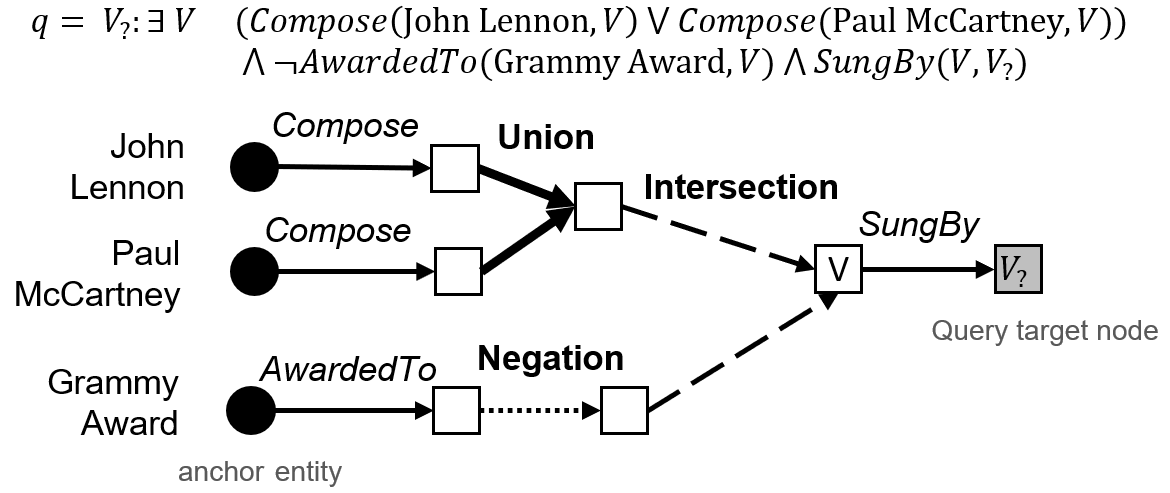
Figure 1: FOL query and its dependency graph for the question ``Who sang the songs that were written by John Lennon or Paul McCartney but never won a Grammy Award?''.

This task is challenging due to the size and the incompleteness of KGs. FOL query answering has been studied as a graph query optimization problem in the database community (Hartig and Heese 2007; Zou et al. 2011; Schmidt, Meier, and Lausen 2010). These methods traverse the KG to retrieve answers for each sub-query and then merge the results. Though being extensively studied, these methods cannot well resolve the above-mentioned challenges. The time complexity exponentially grows with the query complexity and is affected by the size of the intermediate results. This makes them difficult to scale to modern KGs, whose entities are often numbered in millions (Bollacker et al. 2008; Vrandečić and Krötzsch 2014). For example, Wikidata is one of the most influential KGs and reports that their query engine fails when the number of entities in a sub-query (e.g., people born in Germany) exceeds a certain threshold. In addition, real-world KGs are often incomplete, which prevents directly answering many queries by searching KGs. A recent study shows that only 0.5% of football players in Wikidata have a highly complete profile, while over 40% contain only basic information (Balaraman, Razniewski, and Nutt 2018).

To address the challenges of time complexity and KG incompleteness, a line of recent studies (Hamilton et al. 2018; Ren, Hu, and Leskovec 2020; Ren and Leskovec 2020) embed logical queries and entities into the same vector space. The idea is to represent a query using a dependency graph (Figure 1) and embed a complex logical query by iteratively computing embeddings from anchor entities to the target node in a bottom-up manner. The continuous and meaningful entity embeddings empower these approaches to handle missing edges. In addition, these models significantly reduce time and space complexity for inference, as they reduce query answering to dense similarity matching of query and entity embeddings and can speed it up using methods like maximum inner product search (MIPS) (Shrivastava and Li 2014).

These methods nonetheless entail several limitations: First, the logical operators in these models are often defined ad-hoc, and many do not satisfy basic logic laws (e.g., the associative law $(\psi_{1}\land\psi_{2})\land\psi_{3}\equiv\psi_{1}\land(\psi_{2}\land\psi_{3})$ for logical formulae $\psi_{1},\psi_{2},\psi_{3}$), which limits their inference accuracy. Second, the logical operators of existing methods are based on deep architectures, which require many training queries containing such logical operations to learn the parameters. This greatly limits the models' scope of application due to the challenge of collecting numerous reasonable complex queries with accurate answers.

Our goal is to create a logical query embedding framework that satisfies logical laws and provides learning-free logical operators. We hereby present FuzzQE (Fuzzy Query Embedding), a fuzzy logic based embedding framework for answering logical queries on KGs. We borrow the idea of fuzzy logic and use fuzzy conjunction, disjunction, and negation to implement logical operators in a more principled and learning-free manner. Our approach provides the following advantages over existing approaches: (i) FuzzQE employs differentiable logical operators that fully satisfy the axioms of logical operations and can preserve logical operation properties in vector space. This superiority is corroborated by extensive experiments on two benchmark datasets, which demonstrate that FuzzQE delivers a significantly better performance compared to state-of-the-art methods in answering FOL queries. (ii) Our logical operations do not require learning any operator-specific parameters. We conduct experiments to show that even when our model is only trained with link prediction, it achieves better results than state-of-the-art logical query embedding models trained with extra complex query data. This represents a huge advantage in real-world applications since complex FOL training queries are often arduous to collect. In addition, when complex training queries are available, the performance of FuzzQE can be further enhanced.

In addition to proposing this novel and effective framework, we propose some basic properties that a logical query embedding model ought to possess as well as analyze whether existing models can fulfill these conditions. This analysis provides theoretical guidance for future research on embedding-based logical query answering models.

2 Related Work

Embedding entities in Knowledge Graphs (KGs) into continuous embeddings have been extensively studied (Bordes et al. 2013; Yang et al. 2015; Trouillon et al. 2016; Sun et al. 2019), which can answer one-hop relational queries via link prediction. These models, however, cannot handle queries with multi-hop (Guu, Miller, and Liang 2015) or complex logical reasoning. Hamilton et al. (2018) thus propose a graph-query embedding (GQE) framework that encodes a conjunctive query via a dependency graph with relation projection and conjunction ($\land$) as operators. Ren, Hu, and Leskovec (2020) extend GQE by using box embedding to represent entity sets, where they define the disjunction ($\lor$) operator to support Existential Positive First-Order (EPFO) queries. Sun et al. (2020) concurrently propose to represent sets as count-min sketch (Cormode and Muthukrishnan 2005) that can support conjunction and disjunction operators. More recently,  Ren and Leskovec (2020) further include the negation operator ($\neg$) by modeling the query and entity set as beta distributions. Friedman and Van den Broeck (2020) extend FOL query answering to probabilistic databases. These query embedding models have shown promising results to conduct multi-hop logical reasoning over incomplete KGs efficiently regarding time and space; however, we found that these models do not satisfy the axioms of either Boolean logic (Chvalovskỳ 2012) or fuzzy logic (Klement, Mesiar, and Pap 2000), which limits their inference accuracy. To address this issue, our approach draws from fuzzy logic and uses the fuzzy conjunction, disjunction, and negation operations to define the logical operators in the vector space.

In addition to the above logical query embedding models, a recent work CQD (Arakelyan et al. 2021) proposes training an embedding-based KG completion model (e.g., ComplEx (Trouillon et al. 2016)) to impute missing edges during inference and merge entity rankings using t-norms and t-conorms (Klement, Mesiar, and Pap 2000). Using beam search for inference, CQD has demonstrated strong capability of generalizing from KG edges to arbitrary EPFO queries. However, CQD has severe scalability issues since it involves scoring every entity for every atomic query. This is undesirable in real-world applications, since the number of entities in real-world KGs are often in millions (Bollacker et al. 2008; Vrandečić and Krötzsch 2014). Furthermore, its inference accuracy is thus bounded by KG link prediction performance. In contrast, our model is highly scalable, and its performance can be further enhanced when additional complex queries are available for training.

		Logic Law	Model Property
$\land$	I	Conjunction Elimination
		$\psi_{1}\wedge\psi_{2}\rightarrow\psi_{1}$	$\phi(q_{1}\land q_{2},e)\leq\phi(q_{1},e)$
		$\psi_{1}\wedge\psi_{2}\rightarrow\psi_{2}$	$\phi(q_{1}\land q_{2},e)\leq\phi(q_{2},e)$
	II	Commutativity
		$\psi_{1}\land\psi_{2}\leftrightarrow\psi_{2}\land\psi_{1}$	$\phi((q_{1}\land q_{2}),e)=\phi((q_{2}\land q_{1}),e)$
	III	Associativity
		$(\psi_{1}\land\psi_{2})\land\psi_{3}\leftrightarrow\psi_{1}\land(\psi_{2}\land\psi_{3})$	$\phi((q_{1}\land q_{2})\land q_{3},e)=\phi(q_{1}\land(q_{2}\land q_{3}),e)$
$\lor$	IV	Disjunction Amplification
		$\psi_{1}\rightarrow\psi_{1}\vee\psi_{2}$	$\phi(q_{1},e)\leq\phi(q_{1}\lor q_{2},e)$
		$\psi_{2}\rightarrow\psi_{1}\vee\psi_{2}$	$\phi(q_{2},e)\leq\phi(q_{1}\lor q_{2},e)$
	V	Commutativity
		$\psi_{1}\lor\psi_{2}\leftrightarrow\psi_{2}\lor\psi_{1}$	$\phi((q_{1}\lor q_{2}),e)=\phi((q_{2}\lor q_{1}),e)$
	VI	Associativity
		$(\psi_{1}\lor\psi_{2})\lor\psi_{3}\leftrightarrow\psi_{1}\lor(\psi_{2}\lor\psi_{3})$	$\phi((q_{1}\lor q_{2})\lor q_{3},e)=\phi(q_{1}\lor(q_{2}\lor q_{3}),e)$
$\neg$	VII	Involution
		$\neg\neg\psi_{1}\rightarrow\psi_{1}$	$\phi(q,e)=\phi(\neg\neg q,e)$
	VIII	Non-Contradiction
		$\psi_{1}\land\neg\psi_{1}\rightarrow\overline{0}$	$\phi(q,e)\uparrow\quad\Rightarrow\quad\phi(\neg q,e)\downarrow$

Table 1: Here we list eight logic laws (I - VIII) from classical logic (Zimmermann 1991) and give the corresponding properties that a query embedding model should possess. $\psi_{1},\psi_{2},\psi_{3}$ represent logical formulae. $\phi$ denotes the scoring function that estimates the probability that the entity $e$ can answer the query $q$. $\phi(q,e)\uparrow\Rightarrow\phi(\neg q,e)\downarrow$ means $\phi(\neg q,e)$ is monotonically decreasing with regard to $\phi(q,e)$.

	$\land$				$\lor$				$\neg$
	Expressivity (Closed)	Com.	Asso.	Elim.	Expressivity (Closed)	Com.	Asso.	Ampli.	Expressivity (Closed)	Inv.	Non-Contra.
GQE	✓(✓)	✓	✗	✗	✓(✗)	✓	✓	✓	✗	N/A	N/A
Query2Box	✓(✓)	✓	✓	✓	✓(✗)	✓	✓	✓	✗	N/A	N/A
BetaE	✓(✓)	✓	✗	✗	(i) DNF ✓(✗)	✓	✓	✓	✓(✓)	✓	✗
					(ii) DM ✓(✓)	✓	✓	✗
FuzzQE	✓(✓)	✓	✓	✓	✓(✓)	✓	✓	✓	✓(✓)	✓	✓

Table 2: Comparisons of different models regarding the properties of logical operations. Expressivity indicates whether the model can handle such logical operations, and closed indicates whether the embedding is in a closed form. Commu., Asso., Elim., Ampli., Inv. and Non-contra. stand for commutativity, associativity, conjunction elimination, disjunction amplification, involution, and non-contradiction respectively.

3 Preliminaries

A knowledge graph (KG) consists of a set of triples $\langle e_{s},r,e_{o}\rangle$, with $e_{s},e_{o}\in\mathcal{E}$ (the set of entities) denoting the subject and object entities respectively and $r\in\mathcal{R}$ (the set of relations) denoting the relation between $e_{s}$ and $e_{o}$. Without loss of generality, a KG can be represented as a First-Order Logic (FOL) Knowledge Base, where each triple $\langle e_{s},r,e_{o}\rangle$ denotes an atomic formula $r(e_{s},e_{o})$, with $r\in\mathcal{R}$ denoting a binary predicate and $e_{s},e_{o}\in\mathcal{E}$ as its arguments.

We aim to answer FOL queries expressed with existential quantification ($\exists$), conjunction ($\land$), disjunction($\lor$), and negation ($\neg$). The disjunctive normal form (DNF) of an FOL query $q$ is defined as follows:

$$q[V_{?}]\triangleq V_{?}:\exists V_{1},...,V_{k}(v_{11}\land...\land v_{1N_{1}})\lor...\lor(v_{M1}\land...\land v_{MN_{M}})$$

where $V_{?}$ is the target variable of the query, and $V_{1},...,V_{K}$ denote the bound variable nodes. Each $v_{mn}$ ($m=1,...,M,n=1,...,N_{m}$) represents a literal, i.e., a logical atom or the negation of a logical atom:

$$v_{mn}=\begin{cases}r(e,V)&r\in\mathcal{R},e\in\mathcal{E},V\in\{V_{?},V_{1},...,V_{k}\}\\ \neg r(e,V)&r\in\mathcal{R},e\in\mathcal{E},V\in\{V_{?},V_{1},...,V_{k}\}\\ r(V,V^{\prime})&r\in\mathcal{R},V\in\{V_{1},...,V_{k}\}\\ &V^{\prime}\in\{V_{?},V_{1},...,V_{k}\},V\neq V^{\prime}\\ \neg r(V,V^{\prime})&r\in\mathcal{R},V\in\{V_{1},...,V_{k}\}\\ &V^{\prime}\in\{V_{?},V_{1},...,V_{k}\},V\neq V^{\prime}\\ \end{cases}$$

The goal of answering the logical query $q$ is to find a set of entities ${S_{q}}=\{a|a\in\mathcal{E},q[a]~{}\text{holds true}\}$, where $q[a]$ is a logical formula that substitutes the query target variable $V_{?}$ with the entity $a$.

A complex query can be considered as a combination of multiple sub-queries. For example, the query $q[V_{?}]=V_{?}:$ Compose(John Lennon, $V_{?}$) $\land$ Compose(Paul McCartney, $V_{?}$) can be considered as $q_{1}\land q_{2}$, where

$$q_{1}[V_{?}]=V_{?}:\text{Compose(John Lennon},V_{?})$$

$$q_{2}[V_{?}]=V_{?}:\text{\emph{Compose}(Paul McCartney},V_{?}).$$

Formally, we have:

$$S_{q_{1}\land q_{2}} =S_{q_{1}}\cap S_{q_{1}};$$

$$S_{q_{1}\lor q_{2}} =S_{q_{1}}\cup S_{q_{1}};$$

$$S_{\neg q} =S_{q}^{\complement}$$

where $(\cdot)^{\complement}$ denotes set complement.

Notation wise, we use boldfaced notations ${\mathbf{p}_{e}}$ and ${\mathbf{S}_{q}}$ to represent the embedding for entity $e$ and the embedding for $S_{q}$, i.e., the answer entity set for query $q$, respectively. We use $\psi_{1},\psi_{2},\psi_{3}$ to denote logical formulae.

3.1 Logic Laws and Model Properties

The general idea of logical query embedding models is to recursively define the embedding of a query (e.g., $q_{1}\land q_{2}$) based on logical operations on its sub-queries' embeddings (e.g., $q_{1}$ and $q_{2}$). These logical operations have to satisfy logic laws, which serve as additional constraints to learning-based query embedding models. Unfortunately, most existing query embedding models have (partially) neglected these laws, which result in inferior performance.

In this section, we study these logic laws shared by both classical logic and basic fuzzy logic (Zimmermann 1991) and deduce several basic properties that the logical operators should possess. The logic laws and corresponding model properties are summarized in Table 1.

Axiomatic Systems of Logic

Let $\mathcal{L}$ be the set of all the valid logic formulae under a logic system, and $\psi_{1},\psi_{2},\psi_{3}\in\mathcal{L}$ represent logical formulae. $I(\cdot)$ denotes the truth value of a logical formula. The semantics of Boolean Logic are defined by (i) the interpretation $I:\mathcal{L}\rightarrow\{0,1\}$, (ii) the Modus Ponen inference rule ``$\text{from}~{}\psi_{1}~{}\text{and}~{}\psi_{1}\rightarrow\psi_{2}~{}\text{infer}~{}\psi_{2}$'', which characterizes logic implication ($\rightarrow$) as follows:

$$\psi_{1}\rightarrow\psi_{2}\quad\text{holds if and only if}\quad I(\psi_{2})\geq I(\psi_{1})$$

and (iii) a set of axioms written in Hilbert-style deductive systems (Klir and Yuan 1995). Those axioms define other logic connectives via logic implication ($\rightarrow$); for example, the following three axioms characterize the conjunction ($\land$) of Boolean logic (Chvalovskỳ 2012):

$$\psi_{1}\wedge\psi_{2}\rightarrow\psi_{1}$$

$$\psi_{1}\wedge\psi_{2}\rightarrow\psi_{2}$$

$$(\psi_{3}\rightarrow\psi_{1})\rightarrow((\psi_{3}\rightarrow\psi_{2})\rightarrow(\psi_{3}\rightarrow\psi_{1}\wedge\psi_{2}))$$

The first two axioms guarantee that the truth value of $\psi_{1}\wedge\psi_{2}$ never exceeds the truth values of $\psi_{1}$ and $\psi_{2}$, and the last one enforces that $I(\psi_{1}\wedge\psi_{2})=1$ if $I(\psi_{1})=I(\psi_{2})=1$. The three axioms also imply commutativity and associativity of logical conjunction $\land$. More discussions about the axiomatic systems can be found in Appendix B.

Model Properties

Let $\phi(q,e)$ be the embedding model scoring function estimating the probability that the entity $e$ can answer the query $q$. This means that $\phi(q,e)$ estimates the truth value $I(q[e])$, where $q[e]$ is a logical formula that uses $e$ to fill $q$. For example, given the query $q=V_{?}:\emph{Compose}(\emph{John Lennon},V_{?})$ and the entity $e=\emph{``Let it Be''}$, $\phi(q,e)$ estimates the truth value of the logical formula $\emph{Compose}(\emph{John Lennon},\emph{Let it Be})$. We can thus use logic laws to deduce reasonable properties that a query embedding model should possess. For instance, $\psi_{1}\wedge\psi_{2}\rightarrow\psi_{1}$ is an axiom that characterizes logic conjunction ($\land$), which enforces that $I(\psi_{1}\land\psi_{2})\leq I(\psi_{1})$, and we accordingly expect the embedding model to satisfy $\phi(q_{1}\land q_{2},e)\leq\phi(q_{1},e)$, i.e., an entity $e$ is less likely to satisfy $q_{1}\land q_{2}$ than $q_{1}$.

Based on the axioms and deduced logic laws of classical logic (Fodor and Roubens 1994), we summarize a series of model properties that a logical query embedding model should possess in Table 1. The list is not exhaustive but indicative.

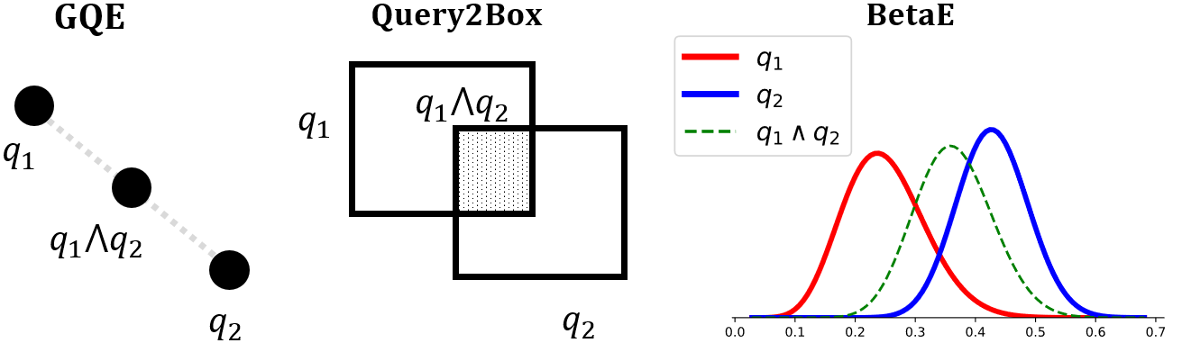
Figure 2: Illustration of query embeddings and embeddings of conjunctive queries in GQE, Query2Box, and BetaE. The conjunction operators takes embeddings of queries $q_{1},q_{2}$ as input and produce an embedding for $q_{1}\land q_{2}$.

3.2 Analysis of Prior Models on Model Properties

This section examines three representative logical query embedding models, namely GQE (Hamilton et al. 2018), Query2Box (Ren, Hu, and Leskovec 2020), and BetaE (Ren and Leskovec 2020), regarding their capability of satisfying the properties in Table 1. We summarize our findings in Table 2. GQE, Query2Box, BetaE represent queries as vectors, boxes (axis-aligned hyper-rectangles), and Beta distributions, respectively. The embedding-based logical operators transform embeddings of sub-queries into embeddings of the outcome query. A brief summary of logical operators of these models are given in Appendix C.

Conjunction ($\land$)

Fig. 2 illustrates embedding-based conjunction operators of the three models, which take embeddings of queries $q_{1},q_{2}$ as input and produce an embedding for $q_{1}\land q_{2}$. GQE, Query2Box, and BetaE are purposely constructed to be permutation invariant (Hamilton et al. 2018; Ren, Hu, and Leskovec 2020; Ren and Leskovec 2020), and their conjunction operators all satisfy commutativity (Law II). The conjunction operators of GQE and BetaE do not satisfy associativity (III) since they rely on the operation of averaging, which is not associative. GQE does not satisfy conjunction elimination (I); for example, supposing that ${\mathbf{p}_{e}}=\frac{1}{2}({\mathbf{S}_{q}}_{1}+{\mathbf{S}_{q}}_{2})$, ${\mathbf{S}_{q}}_{1}\neq{\mathbf{S}_{q}}_{2}$, we have $\phi(q_{1}\land q_{2},e)=\cos({\mathbf{p}_{e}},\frac{1}{2}({\mathbf{S}_{q}}_{1}+{\mathbf{S}_{q}}_{2}))>\cos({\mathbf{p}_{e}},{\mathbf{S}_{q}}_{1})=\phi(q_{1},e)$. BetaE does not satisfy conjunction elimination (I) for similar reasons.

Disjunction ($\lor$)

Previous works handle disjunction in two ways: the Disjunctive Normal Form (DNF) rewriting approach proposed by Query2Box (Ren, Hu, and Leskovec 2020), and the De Morgan's law (DM) approach proposed by BetaE (Ren and Leskovec 2020). The DNF rewriting method involves rewriting each query as a DNF to ensure that disjunction only appears in the last step, which enables the model to simply retain all input embeddings. The model correspondingly cannot represent the disjunction result as a closed form; for example, the disjunction of two boxes remains two separate boxes instead of one (Ren, Hu, and Leskovec 2020). The DM approach uses De Morgan's law $\psi_{1}\lor\psi_{2}\equiv\neg(\neg\psi_{1}\land\neg\psi_{2})$ to compute the disjunctive query embedding, which requires the model to have a conjunction operator and a negation operator. This approach advantageously produces representation in a closed form, allowing disjunction to be performed at any step of the computation. The disadvantage is that if the negation operator does not work well, the error will be amplified and affect disjunction. The DM variant of BetaE, namely BetaE${}_{\text{DM}}$, does not satisfy disjunction amplification (IV) since its negation operator violates non-contradiction (VIII).

Negation

To the best of our knowledge, BetaE is the only previous model that can handle negation. BetaE has proved that its negation operator is involutory (VII) (Ren and Leskovec 2020). However, this operator lacks the non-contradiction property (VIII), as for BetaE $\phi(\neg q,e)$ is not monotonically decreasing with regard to $\phi(q,e)$. An illustration is given in Appendix C.2.

3.3 Fuzzy Logic

Fuzzy logic differs from Boolean logic by associating every logical formula with a truth value in $[0,1]$. Fuzzy logic systems usually retain the axioms of Boolean logic, which ensures that all the logical operation behaviors are consistent with Boolean logic when the truth values are $0$ or $1$. Different fuzzy logic systems add different axioms to define the logical operation behavior for the case when the truth value is in $(0,1)$ (Klir and Yuan 1995). A $t$-norm $\top:[0,1]\times[0,1]\mapsto[0,1]$ represents generalized conjunction in fuzzy logic. Prominent examples of $t$-norms include Gödel t-norm $\top_{\min}\{x,y\}=\min(x,y)$, product t-norm $\top_{\text{prod}}\{x,y\}=xy$, and Łukasiewicz $t$-norm$\top_{Łukasiewicz}(x,y)=\max\{0,x+y-1\}$, for $x,y\in[0,1]$. Any other continuous $t$-norm can be described as an ordinal sum of these three basic ones (Klement, Mesiar, and Pap 2000). Analogously, $t$-conorm are dual to $t$-norms for disjunction in fuzzy logic – given a $t$-norm $\top$, the t-conorm is defined as $\bot(x,y)=1-\top(1-x,1-y)$ based on De Morgan's law and the negator $n(x)=1-x$ for $x,y\in[0,1]$ (Klement, Mesiar, and Pap 2000). This technique has inspired numerous subsequent works. For example, CQD (Arakelyan et al. 2021) uses t-norms and t-conorms to rank entities for query answering on KGs.

4 Methodology

In this section, we propose our model FuzzQE, a framework for answering FOL queries in the presence of missing edges. FuzzQE embeds queries as fuzzy vectors (Katsaras and Liu 1977). Logical operators are implemented via fuzzy conjunction, fuzzy disjunction and fuzzy negation in the embedding space.

4.1 Queries and Entities in Fuzzy Space

Predicting whether an entity can answer a query means predicting the probability that the entity belongs to the answer set of this query. In our work, we embed queries and entities to the fuzzy space $[0,1]^{d}$, a subspace of $\mathbb{R}^{d}$ (Katsaras and Liu 1977).

Query Embedding

Consider a query $q$ and its fuzzy answer set $S_{q}$, its embedding ${\mathbf{S}_{q}}$ is defined as a fuzzy vector ${\mathbf{S}_{q}}\in[0,1]^{d}$ (Katsaras and Liu 1977). Intuitively, let $\Omega$ denote the universe of all the elements, and let $\{U_{i}\}_{i=1}^{d}$ denote a partition over $\Omega$, i.e., $\Omega=\cup_{i=1}^{d}{U_{i}}$ and $U_{i}\cap U_{j}=\emptyset$ for $i\neq j$. Each dimension $i$ of ${\mathbf{S}_{q}}$ denotes the probability whether the corresponding subset $U_{i}$ is part of the answer set $S_{q}$, i.e., ${\mathbf{S}_{q}}(i)=\Pr(U_{i}\subseteq{S_{q}})$.

Entity Embedding

For an entity $e$, we consider its embedding ${\mathbf{p}_{e}}$ from the same fuzzy space, i.e., ${\mathbf{p}_{e}}\in[0,1]^{d}$. To model its uncertainty, we model it as a categorical distribution to fall into each subset $U_{i}$, namely, ${\mathbf{p}_{e}}(i)=\Pr(e\in U_{i})$, and $\sum_{i=1}^{d}{\mathbf{p}_{e}}(i)=1$.

Score Function

Accordingly, the score function $\phi(q,e)$ is defined as the expected probability that $e$ belongs to the fuzzy set $S_{q}$:

$$\phi(q,e) =\mathbb{E}_{e\sim{\mathbf{p}_{e}}}[e\in{S_{q}}]$$

$$=\sum_{i=1}^{d}\Pr(e\in U_{i})\Pr(U_{i}\subseteq{S_{q}})$$

$$={\mathbf{S}_{q}}^{\intercal}{\mathbf{p}_{e}}$$

Note for query embedding in FuzzQE, the all-one vector $\mathbf{1}$ represents the universe set (i.e., $\Omega$), and the all-zero vector $\mathbf{0}$ represents an empty set $\emptyset$.

The above representation and scoring provides the following benefits: (i) The representation is endowed with probabilistic interpretation, and (ii) each dimension of the embedding vector is between $[0,1]$, which satisfies the domain and range requirements of fuzzy logic and allows the model to execute element-wise fuzzy conjunction/disjunction/negation. In light of the fact that $L_{1}$ normalization could impose sparsity on entity embeddings, we also alternatively explore adopting $L_{2}$ normalization to improve embedding learning, i.e., $\sum_{i=1}^{d}{\mathbf{p}_{e}^{2}}(i)=1$.

4.2 Relation Projection for Atomic Queries

Atomic queries like $q=\emph{Compose}(\emph{John Lennon},V_{?})$ serve as building blocks of complex queries. To embed atomic queries, we associate each relation $r\in\mathcal{R}$ with a projection operator $\mathcal{P}_{r}$, which is modeled by a neural network with a weight matrix $\mathbf{W}_{r}\in\mathbb{R}^{d\times d}$ and a bias vector $\mathbf{b}_{r}\in\mathbb{R}^{d}$, and transforms an anchor entity embedding ${\mathbf{p}_{e}}$ into a query embedding:

$${\mathbf{S}_{q}}=\mathcal{P}_{r}({\mathbf{p}_{e}})=\mathbf{g}(\text{LN}(\mathbf{W}_{r}{\mathbf{p}_{e}}+\mathbf{b}_{r}))$$

where LN is Layer Normalization (Ba, Kiros, and Hinton 2016), and $\mathbf{g}:\mathbb{R}^{d}\mapsto[0,1]^{d}$ is a mapping function that constrains ${\mathbf{S}_{q}}\in[0,1]^{d}$. Particularly, we consider two different choices for $\mathbf{g}$:

$$\text{Logistic function}: ~{}\mathbf{g}(\mathbf{x})=\frac{1}{1+e^{-(\mathbf{x})}}$$

$$\text{Bounded rectifier}: ~{}\mathbf{g}(\mathbf{x})=\min(\max(\mathbf{x},0),1)$$

We follow (Schlichtkrull et al. 2018) and adopt basis-decomposition to define $\mathbf{W}_{r}$ and $\mathbf{b}_{r}$:

$$\mathbf{W}_{r}=\sum_{j=1}^{K}\alpha_{rj}\mathbf{M}_{j};\quad\mathbf{b}_{r}=\sum_{j=1}^{K}\alpha_{rj}\mathbf{v}_{j}$$

Namely, $\mathbf{W}_{r}$ as a linear combination of $K$ basis transformations $\mathbf{M}_{j}\in\mathbb{R}^{d\times d}$ with coefficients $\alpha_{rj}$ that depend on $r$. Similarly, $\mathbf{b}_{r}$ is a linear combination of $K$ basis vectors $\mathbf{v}_{j}\in\mathbb{R}^{d}$ with coefficients $\alpha_{rj}$. This form prevents the rapid growth in the number of parameters with the number of relations and alleviates overfitting on rare relations. It can be seen as a form of effective weight sharing among different relation types (Schlichtkrull et al. 2018). Atomic queries that project from one set to another can be embedded similarly.

In principle, any sufficiently expressive neural network or translation-based KG embedding model (Bordes et al. 2013; Ji et al. 2015) could be employed as the relation projection operator in our framework.

4.3 Fuzzy Logic Based Logical Operators

Fuzzy logic is mathematically equivalent to fuzzy set theory (Klir and Yuan 1995), with fuzzy conjunction equivalent to fuzzy set intersection, fuzzy disjunction equivalent to fuzzy set union, and fuzzy negation to fuzzy set complement. Fuzzy logic could thus be used to define operations over fuzzy vectors. As discussed in Section 3.3, the three most prominent $t$-norm based logic systems are product logic, Gödel logic, and Łukasiewicz logic (Klement, Mesiar, and Pap 2000). With reference to product logic, FuzzQE computes the embeddings of $q_{1}\land q_{2}$, $q_{1}\lor q_{2}$, and $\neg q$ as follows:

$$q_{1}\land q_{2}: \quad\mathcal{C}({\mathbf{S}_{q}}_{1},{\mathbf{S}_{q}}_{2}) ={\mathbf{S}_{q}}_{1}\circ{\mathbf{S}_{q}}_{2}$$

$$q_{1}\lor q_{2}: \quad\mathcal{D}({\mathbf{S}_{q}}_{1},{\mathbf{S}_{q}}_{2}) ={\mathbf{S}_{q}}_{1}+{\mathbf{S}_{q}}_{2}-{\mathbf{S}_{q}}_{1}\circ{\mathbf{S}_{q}}_{2}$$

$$\neg q: \quad\mathcal{N}({\mathbf{S}_{q}}) =\mathbf{1}-{\mathbf{S}_{q}}$$

where $\circ$ denotes element-wise multiplication (fuzzy conjunction), $\mathbf{1}$ is the all-one vector, and $\mathcal{C},\mathcal{D},\mathcal{N}$ denote the embedding based logical operators respectively.

Alternatively, the conjunction and disjuction operators can be designed based on Gödel logic as follows:

$$q_{1}\land q_{2}: \quad\mathcal{C}({\mathbf{S}_{q}}_{1},{\mathbf{S}_{q}}_{2}) =\min({\mathbf{S}_{q}}_{1},{\mathbf{S}_{q}}_{2})$$

$$q_{1}\lor q_{2}: \quad\mathcal{D}({\mathbf{S}_{q}}_{1},{\mathbf{S}_{q}}_{2}) =\max({\mathbf{S}_{q}}_{1},{\mathbf{S}_{q}}_{2})$$

where $\min,\max$ denotes element-wise minimum and maximum operation respectively.

We omit Łukasiewicz logic here since its output domain is heavily concentrated in $\{0,1\}$, which causes a query embedding learning problem. More discussions about these three logic systems can be found in Appendix F.

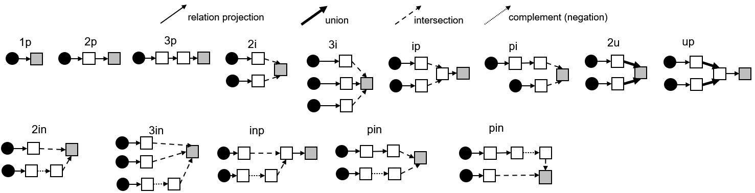
Figure 3: Query structure types in the datasets provided by BetaE (Ren and Leskovec 2020). Naming convention: $p$ for relation projection, $i$ for conjunction (intersection), $n$ for negation (complement), $u$ for disjunction (union). $10$ query structures are used for both training and evaluation: 1p, 2p, 3p, 2i, 3i, 2in, 3in, inp, pni, pin. In order to test the generalization capability of the model, 4 query structures (ip, pi, 2u, up) are not present in training and only included for evaluation.

4.4 Model Learning and Inference

Given a query $q$, we optimize the following objective:

$$L=-\log\sigma(\frac{1}{Z_{q}}\phi(q,e)-\gamma)-\frac{1}{k}\sum_{i=1}^{k}\log\sigma(\gamma-\frac{1}{Z_{q}}\phi(q,e^{\prime}))$$

where $e\in S_{q}$ is an answer to the query, $e^{\prime}\notin{S_{q}}$ represents a random negative sample, and $\gamma$ denotes the margin. $Z_{q}$ is an $L_{2}$ norm based scaling factor, which is introduced as a means to balance margin sensitivity between queries during training. In the loss function, we use $k$ random negative samples and optimize the average. We seek to maximize $\phi(q,e)$ for $e\in S_{q}$ and minimize $\phi(q,e^{\prime})$ for $e^{\prime}\in S_{q}$.

For the model inference, given a query $q$, FuzzQE embeds it as ${\mathbf{S}_{q}}$ and rank all the entities by $\phi(q,\cdot)$.

4.5 Theoretical Analysis

For FuzzQE, we present the following propositions with proof in Appendix A.

Proposition 1.

Our conjunction operator $\mathcal{C}$ is commutative, associative, and satisfies conjunction elimination.

Proposition 2.

Our disjunction operator $\mathcal{D}$ is commutative, associative, and satisfies disjunction amplification.

Proposition 3.

Our negation operator $\mathcal{N}$ is involutory and satisfies non-contradiction.

5 Experiments

Type of Model	Model	Avg${}_{\text{EPFO}}$	Avg${}_{\text{Neg}}$	1p	2p	3p	2i	3i	pi	ip	2u	up	2in	3in	inp	pin	pni
FB15k-237
Query Embedding	GQE	16.3	N/A	35.0	7.2	5.3	23.3	34.6	16.5	10.7	8.2	5.7	N/A	N/A	N/A	N/A	N/A
	Query2Box	20.1	N/A	40.6	9.4	6.8	29.5	42.3	21.2	12.6	11.3	7.6	N/A	N/A	N/A	N/A	N/A
	BetaE	20.9	5.5	39.0	10.9	10.0	28.8	42.5	22.4	12.6	12.4	9.7	5.1	7.9	7.4	3.5	3.4
	FuzzQE	24.2	8.5	42.2	13.3	10.2	33.0	47.3	26.2	18.9	15.6	10.8	9.7	12.6	7.8	5.8	6.6
Query Optimization	CQD	21.7	N/A	46.3	9.9	5.9	31.7	41.3	21.8	15.8	14.2	8.6	N/A	N/A	N/A	N/A	N/A
NELL995
Query Embedding	GQE	18.6	N/A	32.8	11.9	9.6	27.5	35.2	18.4	14.4	8.5	8.8	N/A	N/A	N/A	N/A	N/A
	Query2Box	22.9	N/A	42.2	14.0	11.2	33.3	44.5	22.4	16.8	11.3	10.3	N/A	N/A	N/A	N/A	N/A
	BetaE	24.6	5.9	53.0	13.0	11.4	37.6	47.5	24.1	14.3	12.2	8.5	5.1	7.8	10.0	3.1	3.5
	FuzzQE	29.3	8.0	58.1	19.3	15.7	39.8	50.3	28.1	21.8	17.3	13.7	8.3	10.2	11.5	4.6	5.4
Query Optimization	CQD	28.4	N/A	60.0	16.5	10.4	40.4	49.6	27.6	20.8	16.8	12.6	N/A	N/A	N/A	N/A	N/A

Table 3: MRR results (%) on answering FOL queries. We report MRR results (%) on test FOL queries. Avg${}_{\text{EPFO}}$ and Avg${}_{\text{Neg}}$ denote the average MRR on EPFO queries (queries with $\exists,\land,\lor$ and without negation) and queries containing negation respectively. Results of GQE, Query2Box, and BetaE are taken from (Ren and Leskovec 2020).

Model	Avg${}_{\text{EPFO}}$	Avg${}_{\text{Neg}}$	1p	2p	3p	2i	3i	pi	ip	2u	up	2in	3in	inp	pin	pni
FB15k-237
GQE	17.7	N/A	41.6	7.9	5.4	25.0	33.6	16.3	10.9	11.9	6.2	N/A	N/A	N/A	N/A	N/A
Query2Box	18.2	N/A	42.6	6.9	4.7	27.3	36.8	17.5	11.1	11.7	5.5	N/A	N/A	N/A	N/A	N/A
BetaE	15.8	0.5	37.7	5.6	4.4	23.3	34.5	15.1	7.8	9.5	4.5	0.1	1.1	0.8	0.1	0.2
FuzzQE	21.8	6.6	44.0	10.8	8.6	32.3	41.4	22.7	15.1	13.5	8.7	7.7	9.5	7.0	4.1	4.7
NELL995
GQE	21.7	N/A	47.2	12.7	9.3	30.6	37.0	20.6	16.1	12.6	9.6	N/A	N/A	N/A	N/A	N/A
Query2Box	21.6	N/A	47.6	12.5	8.7	30.7	36.5	20.5	16.0	12.7	9.6	N/A	N/A	N/A	N/A	N/A
BetaE	19.0	0.4	53.1	6.0	3.9	32.0	37.7	15.8	8.5	10.1	3.5	0.1	1.4	0.1	0.1	0.1
FuzzQE	27.1	7.3	57.6	17.2	13.3	38.2	41.5	27.0	19.4	16.9	12.7	9.1	8.3	8.9	4.4	5.6

Table 4: MRR results (%) of logical query embedding models that are trained with only link prediction. This task tests the ability of the model to generalize to arbitrary complex logical queries, when no complex logical query data is available for training. Avg${}_{\text{EPFO}}$ and Avg${}_{\text{Neg}}$ denote the average MRR on EPFO ($\exists,\land,\lor$) queries and queries containing negation respectively.

In this section, we evaluate the ability of FuzzQE  to answer complex FOL queries over incomplete KGs.

5.1 Evaluation Setup

Datasets

We evaluate our model on two benchmark datasets provided by (Ren and Leskovec 2020), which contain 14 types of logical queries on FB15k-237 (Toutanova and Chen 2015) and NELL995 (Xiong, Hoang, and Wang 2017) respectively. The 14 types of query structures in the datasets are shown in Fig. 3. Note that these datasets provided by BetaE (Ren and Leskovec 2020) are an improved and expanded version of the datasets provided by Query2Box (Ren, Hu, and Leskovec 2020). Compared to the earlier version, the new datasets Ren and Leskovec (2020) contain 5 new types of queries that involve negation. The validation/test set of the original 9 query types are regenerated to ensure that the number of answers per query is not excessive, making this task more challenging. In the new datasets, $10$ query structures are used for both training and evaluation: $1p,2p,3p,2i,3i,2in,3in,inp,pni,pin$. $4$ query structures ($ip,pi,2u,up$) are not used for training but only included in evaluation in order to evaluate the model's generalization ability of answering queries with logical structures that the model has never seen during training. We exclude FB15k (Bordes et al. 2013) since this dataset suffers from major test leakage (Toutanova and Chen 2015). Statistics about the datasets are summarized in Appendix D.

Evaluation Protocol

We follow the evaluation protocol in (Ren and Leskovec 2020). To evaluate the model's generalization capability over incomplete KGs, the datasets are masked out so that each validation/test query answer pair involves imputing at least one missing edge. For each answer of a test query, we use the Mean Reciprocal Rank (MRR) as the major evaluation metric. We use the filtered setting (Bordes et al. 2013) and filter out other correct answers from ranking before calculating the MRR.

Baselines and Model Configurations

We consider three logical query embedding baselines for answering complex logical queries on KGs: GQE (Hamilton et al. 2018), Query2Box (Ren, Hu, and Leskovec 2020), and BetaE (Ren and Leskovec 2020). We also compare with one recent state-of-the-art query optimization model CQD (Arakelyan et al. 2021). For GQE, Query2Box, and BetaE we use implementation provided by (Ren and Leskovec 2020) . For BetaE and CQD, we compare with the model variant that generally provides better performance, namely BetaE${}_{\text{DNF}}$ and CQD-BEAM. CQD cannot process complex logical queries during training and is thus trained with KG edges. To the best of our knowledge, BetaE is the only available baseline that can handle negation. Therefore, for GQE, Query2Box, and CQD, we compare with them only on EPFO queries (queries with $\exists,\land,\lor$ and without negation).

For FuzzQE, we report results using the logic system that provide the best average MRR on the validation set. we use AdamW (Loshchilov and Hutter 2019) as the optimizer. Training terminates with early stopping based on the average MRR on the validation set with a patience of 15k steps. We repeat each experiment three times with different random seeds and report the average results. Hyperparameters and more experimental details are given in Appendix E.

5.2 Main Results: Trained with FOL queries

We first test the ability of FuzzQE to model arbitrary FOL queries when complex logical queries are available for training. Results are reported in Table 3.

Comparison with Query Embedding

As shown in Table 3, FuzzQE consistently outperforms all the logical query embedding baselines. For EPFO queries, FuzzQE improves the average MRR of best baseline BetaE (Ren and Leskovec 2020) by 3.3% (ca. 15% relative improvement) on FB15k-237 and 4.7% (ca. 19% relative improvement) on NELL995. For queries with negation, FuzzQE significantly outperforms the only available baseline BetaE. On average, FuzzQE improves the MRR by 3.0% (54% relatively) on FB15k-237 and 2.1% (36% relatively) on NELL995 for queries containing negation. We hypothesize that this significant enhancement comes from the principled design of our negation operator that satisfies the axioms, while BetaE fails to satisfy the non-contradiction property.

Comparison with Query Optimization: CQD

We next compare FuzzQE with a recent query optimization baseline, CQD (Arakelyan et al. 2021) on EPFO queries. On average, FuzzQE provides 2.5% and 0.9% absolute improvement in MRR on FB15k-237 and NELL995 respectively. It is worth noting that FuzzQE outperforms CQD on most complex query structures on NELL995 even with slightly worse $1p$ query answering performance. We hypothesize that the $1p$ query answering performance difference on NELL995 comes from the differenct abilities of different relation projection/link prediction models to encode sparse knowledge graphs.

A major motivation for learning logical query embedding is its high inference efficiency. We compare with CQD with regard to the time for answering a query. On a $\text{NVIDIA}^{\circledR}$ GP102 TITAN Xp (12GB), the average time for CQD to answer a FOL query on FB15k-237 is 13.9 ms (milliseconds), while FuzzQE takes only 0.3 ms. On NELL995, where the number of entities is 4 times the number in FB15k-237, the average time for CQD is 68.1 ms, whereas FuzzQE needs only 0.4 ms. CQD takes 170 times longer than FuzzQE. The reason is that CQD is required to score all the entities for each subquery to obtain the top-$k$ candidates for beam search.

5.3 Trained with only Link Prediction

This experiment tests the ability of the model to generalize to arbitrary complex logical queries when it is trained with only the link prediction task. To evaluate it, we train FuzzQE and other logical query embedding models using only KG edges (i.e., 1p queries). For baseline models GQE, Query2Box, and BetaE, we adapt them following the experiment settings of the Q2B-AVG-1P model discussed in (Ren, Hu, and Leskovec 2020). Specifically, we set all the sub-query weights to $1.0$ for this experiment.

As shown in Table 4, FuzzQE is able to generalize to complex logical queries of new query structures even if it is trained on link prediction and provides significantly better performance than baseline models. Compared to the best baseline, FuzzQE improves the average MRR by 3.6% (20% relatively) for EPFO queries on FB15k-237 and 5.4% (26% relatively) on NELL995. Regarding queries with negation, our model drastically outperforms the only available baseline BetaE across datasets. In addition, compared with the ones trained with complex FOL queries (in Table 3), It is worth nothing that FuzzQE trained with only link prediction can outperform BetaE models that are trained with extra complex logical queries in terms of average MRR (in Table 3). This demonstrates the superiority of the logical operators in FuzzQE, which are designed in a principled and learning-free manner. Meanwhile, FuzzQE can still take advantage of additional complex queries as training samples to enhance entity embeddings.

6 Conclusion

We propose a novel logical query embedding framework FuzzQE for answering complex logical queries on KGs. Our model FuzzQE borrows operations from fuzzy logic and implements logical operators in a principled and learning-free manner. Extensive experiments show the promising capability of FuzzQE on answering logical queries on KGs. The results are encouraging and suggest various extensions, including introducing logical rules into embedding learning, as well as studying the potential use of predicate fuzzy logic systems and other deeper transformation architectures. Future research could also use the defined logical operators to incorporate logical rules to enhance reasoning on KGs. Furthermore, we are interested in jointly learning embeddings for logical queries, natural language questions, entity labels to enhance question answering on KGs.

Appendix

Appendix A Proof of propositions

We hereby provide proof of propositions for FuzzQE using product logic. The same can be proved for Gödel logic.

A.1 Proof of Proposition 1

Commutativity $\phi(q_{1}\land q_{2},e)=\phi(q_{2}\land q_{1},e)$

Proof.

We have $\mathcal{C}({\mathbf{S}_{q}}_{1},{\mathbf{S}_{q}}_{2})=q_{1}\circ q_{2}=q_{2}\circ q_{1}=\mathcal{C}({\mathbf{S}_{q}}_{2},{\mathbf{S}_{q}}_{1})$ where $\circ$ denotes element-wise multiplication.
Therefore, $\phi(q_{1}\land q_{2},e)={\mathbf{p}_{e}}^{\intercal}\mathcal{C}({\mathbf{S}_{q}}_{1},{\mathbf{S}_{q}}_{2})={\mathbf{p}_{e}}^{\intercal}\mathcal{C}({\mathbf{S}_{q}}_{2},{\mathbf{S}_{q}}_{1})=\phi(q_{2}\land q_{1},e)$. ∎

Associativity $\phi((q_{1}\land q_{2})\land q_{3},e)=\phi(q_{1}\land(q_{2}\land q_{3}),e)$

Proof.

Since $\mathcal{C}(\mathcal{C}({\mathbf{S}_{q}}_{1},{\mathbf{S}_{q}}_{2})),{\mathbf{S}_{q}}_{3})=q_{1}\circ q_{2}\circ q_{3}=\mathcal{C}({\mathbf{S}_{q}}_{1},\mathcal{C}({\mathbf{S}_{q}}_{2},{\mathbf{S}_{q}}_{3}))$, we have

$$\phi((q_{1}\lor q_{2})\lor q_{3},e)$$

$$= {\mathbf{p}_{e}}^{\intercal}\mathcal{C}(\mathcal{C}({\mathbf{S}_{q}}_{1},{\mathbf{S}_{q}}_{2})),{\mathbf{S}_{q}}_{3})$$

$$= {\mathbf{p}_{e}}^{\intercal}\mathcal{C}({\mathbf{S}_{q}}_{1},\mathcal{C}({\mathbf{S}_{q}}_{2},{\mathbf{S}_{q}}_{3}))$$

$$= \phi(q_{1}\lor(q_{2}\lor q_{3}),e)$$

∎

Conjunction elimination $\phi(q_{1}\land q_{2},e)\leq\phi(q_{1},e)$,  $\phi(q_{1}\land q_{2},e)\leq\phi(q_{2},e)$

Proof.

$\phi(q_{1}\land q_{2},e)\leq\phi(q_{1},e)$ can be proved by

$$\phi(q_{1}\land q_{2},e)$$

$$= {\mathbf{p}_{e}}^{\intercal}\mathcal{C}({\mathbf{S}_{q}}_{1},{\mathbf{S}_{q}}_{2})$$

$$= {\mathbf{p}_{e}}^{\intercal}({\mathbf{S}_{q}}_{1}\circ{\mathbf{S}_{q}}_{2})$$

$$= \sum_{i=1}^{d}{\mathbf{p}_{e}}_{i}{\mathbf{S}_{q}}_{1_{i}}{\mathbf{S}_{q}}_{2_{i}}$$

$$\leq \sum_{i=1}^{d}{\mathbf{p}_{e}}_{i}{\mathbf{S}_{q}}_{1_{i}}$$

$$= \phi(q_{1},e)$$

$\phi(q_{1}\land q_{2},e)\leq\phi(q_{2},e)$ can be proved similarly. ∎

A.2 Proof of Proposition 2

Commutativity $\phi(q_{1}\lor q_{2},e)=\phi(q_{2}\lor q_{1},e)$

Proof.

We have $\mathcal{D}({\mathbf{S}_{q}}_{1},{\mathbf{S}_{q}}_{2})={\mathbf{S}_{q}}_{1}+{\mathbf{S}_{q}}_{2}-{\mathbf{S}_{q}}_{1}\circ{\mathbf{S}_{q}}_{2}={\mathbf{S}_{q}}_{2}+{\mathbf{S}_{q}}_{1}-{\mathbf{S}_{q}}_{2}\circ{\mathbf{S}_{q}}_{1}=\mathcal{D}({\mathbf{S}_{q}}_{2},{\mathbf{S}_{q}}_{1})$.
Therefore, $\phi(q_{1}\lor q_{2},e)={\mathbf{p}_{e}}^{\intercal}\mathcal{D}({\mathbf{S}_{q}}_{1},{\mathbf{S}_{q}}_{2})={\mathbf{p}_{e}}^{\intercal}\mathcal{D}({\mathbf{S}_{q}}_{2},{\mathbf{S}_{q}}_{1})=\phi(q_{2}\lor q_{1},e)$. ∎

Associativity $\phi((q_{1}\land q_{2})\land q_{3},e)=\phi(q_{1}\land(q_{2}\land q_{3}),e)$

Proof.

$$\mathcal{D}(\mathcal{D}({\mathbf{S}_{q}}_{1},{\mathbf{S}_{q}}_{2})),{\mathbf{S}_{q}}_{3})$$

$$= \mathcal{D}({\mathbf{S}_{q}}_{1}+{\mathbf{S}_{q}}_{2}-{\mathbf{S}_{q}}_{1}\circ{\mathbf{S}_{q}}_{2},{\mathbf{S}_{q}}_{3})$$

$$= ({\mathbf{S}_{q}}_{1}+{\mathbf{S}_{q}}_{2}-{\mathbf{S}_{q}}_{1}\circ{\mathbf{S}_{q}}_{2})+{\mathbf{S}_{q}}_{3}-({\mathbf{S}_{q}}_{1}+{\mathbf{S}_{q}}_{2}-{\mathbf{S}_{q}}_{1}\circ{\mathbf{S}_{q}}_{2})\circ{\mathbf{S}_{q}}_{3}$$

$$= {\mathbf{S}_{q}}_{1}+{\mathbf{S}_{q}}_{2}+{\mathbf{S}_{q}}_{3}-{\mathbf{S}_{q}}_{1}\circ{\mathbf{S}_{q}}_{2}-{\mathbf{S}_{q}}_{1}\circ{\mathbf{S}_{q}}_{3}-{\mathbf{S}_{q}}_{2}\circ{\mathbf{S}_{q}}_{3}+{\mathbf{S}_{q}}_{1}\circ{\mathbf{S}_{q}}_{2}\circ{\mathbf{S}_{q}}_{3}$$

$$= \mathcal{D}({\mathbf{S}_{q}}_{1},\mathcal{D}({\mathbf{S}_{q}}_{2},{\mathbf{S}_{q}}_{3}))$$

Therefore

$$\phi((q_{1}\lor q_{2})\lor q_{3},e)$$

$$= {\mathbf{p}_{e}}^{\intercal}\mathcal{D}(\mathcal{D}({\mathbf{S}_{q}}_{1},{\mathbf{S}_{q}}_{2})),{\mathbf{S}_{q}}_{3})$$

$$= {\mathbf{p}_{e}}^{\intercal}\mathcal{D}({\mathbf{S}_{q}}_{1},\mathcal{D}({\mathbf{S}_{q}}_{2},{\mathbf{S}_{q}}_{3}))$$

$$= \phi(q_{1}\lor(q_{2}\lor q_{3}),e)$$

∎

Disjunction amplification $\phi(q_{1}\lor q_{2},e)\geq\phi(q_{1},e)$,  $\phi(q_{1}\lor q_{2},e)\geq\phi(q_{2},e)$

Proof.

$\phi(q_{1}\lor q_{2},e)\geq\phi(q_{1},e)$ can be proved by

$$\phi(q_{1}\lor q_{2},e)$$

$$= {\mathbf{p}_{e}}^{\intercal}\mathcal{D}({\mathbf{S}_{q}}_{1},{\mathbf{S}_{q}}_{2})$$

$$= {\mathbf{p}_{e}}^{\intercal}({\mathbf{S}_{q}}_{1}+{\mathbf{S}_{q}}_{2}-{\mathbf{S}_{q}}_{1}\circ{\mathbf{S}_{q}}_{2})$$

$$= \sum_{i=1}^{d}{\mathbf{p}_{e}}_{i}({\mathbf{S}_{q}}_{1_{i}}+{\mathbf{S}_{q}}_{2_{i}}-{\mathbf{S}_{q}}_{1_{i}}{\mathbf{S}_{q}}_{2_{i}})$$

$$= \sum_{i=1}^{d}{\mathbf{p}_{e}}_{i}{\mathbf{S}_{q}}_{1_{i}}+{\mathbf{p}_{e}}_{i}{\mathbf{S}_{q}}_{2_{i}}(1-{\mathbf{S}_{q}}_{1_{i}})$$

$$\geq \sum_{i=1}^{d}{\mathbf{p}_{e}}_{i}{\mathbf{S}_{q}}_{1_{i}}$$

$$= \phi(q_{1},e)$$

$\phi(q_{1}\lor q_{2},e)\geq\phi(q_{2},e)$ can be proved similarly. ∎

A.3 Proof of Proposition 3

Involution $\phi(q,e)=\phi(\neg\neg q,e)$

Proof.

$$\mathcal{N}(\mathcal{N}(q))=\mathbf{1}-(\mathbf{1}-{\mathbf{S}_{q}})={\mathbf{S}_{q}}$$

Therefore $\phi(\neg\neg q,e)={\mathbf{p}_{e}}^{\intercal}\mathcal{N}(\mathcal{N}({\mathbf{S}_{q}}))=\phi(q,e)$ ∎

Non-contradiction $\phi(q,e)\uparrow\Rightarrow\phi(\neg q,e)\downarrow$ 

Proof.

The Łukasiewicz negation $c(x)=1-x$ is monotonically decreasing with regard to $x$. Therefore, $\phi(\neg q,e)$ is monotonically decreasing with regard to $\phi(q,e)$. ∎

Appendix B Axiomatic systems of logic

Axiomatic systems of logic consist of a set of axioms and the Modus Ponen inference rule: $\text{from}~{}\varphi~{}\text{and}~{}\varphi\rightarrow\psi~{}\text{infer}~{}\psi$. Implication $\rightarrow$ is defined as $\varphi\rightarrow\psi$ holds if the truth value of $\psi$ is larger than or equal to $\varphi$. In Table 5, we compare the semantics of classical logic and product logic and show that product logic operations are fully compatible with classical logic. In Table 6, we provide the list of axioms written in Hilbert-style deductive system for classical logic, and three prominent fuzzy logic systems: Łukasiewicz logic, Gödel logic, and product logic (Klement, Mesiar, and Pap 2000). We also provide some of the derivable logic laws. Interested readers are referred to (Zimmermann 1991) for proofs.

Table 5: Semantics of classical logic and product logic. $F_{mL}$ denote all valid logic formulae under the logic system, and $\varphi,\psi\in F_{mL}$ are logical formulae. $I(\cdot)$ denotes the truth value of a logical formula.

	Classical Logic	Product Logic
Interpretation $I$	$I:F_{mL}\rightarrow\{0,1\}$	$I:F_{mL}\rightarrow[0,1]$
$I(\varphi\land\psi)$	$I(\varphi)I(\psi)$	$I(\varphi)I(\psi)$
$I(\varphi\lor\psi)$	$I(\varphi)+I(\psi)-I(\varphi)I(\psi)$	$I(\varphi)+I(\psi)-I(\varphi)I(\psi)$
$I(\varphi\rightarrow\psi)$	$\left\{\begin{array}[]{lr}1,\quad\text{if}~{}I(\varphi)\leq I(\psi)\\ I(\psi),\quad\text{otherwise}\end{array}\right.$	$\left\{\begin{array}[]{lr}1,\quad\text{if}I(\varphi)\leq I(\psi)\\ I(\psi),\quad\text{otherwise}\end{array}\right.$

Table 6: Axioms and derivable logic laws of classical logic, basic fuzzy logic, and three prominent fuzzy logic systems that are based on on basic fuzzy logic: Łukasiewicz logic, Gödel logic, and product logic (Klement, Mesiar, and Pap 2000). • denotes that the formula is in the minimal axiomatic system (Chvalovskỳ 2012), while ◦ means the logic law could be derived from the minimal axiomatic system. EFQ stands for Ex falso quodlibet, which is Latin for from falsehood, anything. Strong conjunction of fuzzy logic is usually defined by $t$-norm (See Appendix F) and denoted by $\&$ in literature. Here, to make it easier to compare with classical logic, we uniformly use $\land$ in the axioms.

	Axiom / Logic Law	Classical Logic	Basic Fuzzy Logic	Łukasiewicz	Gödel	Product
Transitivity	$(\varphi\rightarrow\chi)\rightarrow((\psi\rightarrow\chi)\rightarrow(\varphi\rightarrow\chi))$	•	•	•	•	•
Weakening	$\varphi\rightarrow(\psi\rightarrow\varphi)$	•	•	•	•	•
Exchange	$(\varphi\rightarrow(\psi\rightarrow\chi))\rightarrow(\psi\rightarrow(\varphi\rightarrow\chi))$	•	•	•	•	•
$\land$(I)	$\varphi\wedge\psi\rightarrow\varphi$	•	•	•	•	•
$\land$(II)	$\varphi\wedge\psi\rightarrow\psi$	•	•	•	•	•
$\land$(III)	$(\chi\rightarrow\varphi)\rightarrow((\chi\rightarrow\psi)\rightarrow(\chi\rightarrow\varphi\wedge\psi))$	•	•	•	•	•
$\lor$(I)	$\varphi\lor\psi\rightarrow\varphi$	•	•	•	•	•
$\lor$(II)	$\varphi\lor\psi\rightarrow\psi$	•	•	•	•	•
$\lor$(III)	$(\chi\rightarrow\varphi)\rightarrow((\chi\rightarrow\psi)\rightarrow(\chi\rightarrow\varphi\lor\psi))$	•	•	•	•	•
Prelinearity	$(\varphi\rightarrow\psi)\lor(\psi\rightarrow\varphi)$	•	•	•	•	•
EFQ	$\overline{0}\rightarrow\varphi$	•	•	•	•	•
	$\varphi\land\psi\leftrightarrow\psi\land\varphi$	◦	◦	◦	◦	◦
	$(\varphi\land\psi)\land\chi\leftrightarrow\varphi\land(\psi\land\chi)$	◦	◦	◦	◦	◦
	$\varphi\lor\psi\leftrightarrow\psi\lor\varphi$	◦	◦	◦	◦	◦
	$(\varphi\lor\psi)\lor\chi\leftrightarrow\varphi\lor(\psi\lor\chi)$	◦	◦	◦	◦	◦
Contraction	$(\varphi\rightarrow(\varphi\rightarrow\psi))\rightarrow(\varphi\rightarrow\psi)$	◦			•
Wajsberg	$\neg\neg\varphi\rightarrow\varphi$	◦		•
	$\varphi\land\neg\varphi\rightarrow\overline{0}$	◦				•
XI	$\neg\neg\chi\rightarrow(((\varphi\land\chi)\rightarrow(\psi\land\chi))\rightarrow(\phi\rightarrow\psi))$	◦				•

Appendix C Logical Operators of GQE, Query2Box, and BetaE

C.1 Conjunction

GQE, Query2Box, BetaE represent queries as vectors, boxes (axis-aligned hyper-rectangles), and Beta distributions, respectively. Fig. 2 illustrates embedding-based conjunction operators of the three models, which takes embeddings of queries $q_{1},q_{2}$ as input and produce an embedding for $q_{1}\land q_{2}$. Our analysis in Section 3.2 focuses on the nature of the geometry operations, and we thus omit deep architectures of the logical operators of these models from our analysis, such as the attention mechanism or deep sets (Zaheer et al. 2017) for weighing sub-queries. We assume all the sub-queries should have identical weights. The details about the original implementation are given below.

GQE

$$\mathcal{C}({\mathbf{S}_{q}}_{1},{\mathbf{S}_{q}}_{2})=\Psi(\text{NN}_{k}({\mathbf{S}_{q}}_{1},{\mathbf{S}_{q}}_{2}))$$

where ${\mathbf{S}_{q}}_{1},{\mathbf{S}_{q}}_{2}\in\mathbb{R}^{d}$, $\text{NN}_{k}$ is a $k$-layer feedforward neural network, $\Psi$ is a symmetric vector function, usually defined as the element-wise mean (Ren, Hu, and Leskovec 2020).

Query2Box

In Query2Box, each query is represented by $d$ boxes, i.e., a vector ${\mathbf{S}_{q}}_{\text{CEN}}\in\mathbb{R}^{d}$ for box centers and a vector ${\mathbf{S}_{q}}_{\text{OFF}}\in\mathbb{R}^{+d}$ for box sizes. The conjunction operator $\mathcal{C}_{\text{CEN}},\mathcal{C}_{\text{OFF}}$ are defined as follows:

$$\mathcal{C}_{\text{CEN}}({\mathbf{S}_{q}}_{1},{\mathbf{S}_{q}}_{2}) =w_{1}{\mathbf{S}_{q}}_{\text{CEN}1}+w_{2}{\mathbf{S}_{q}}_{\text{CEN}1};\quad w_{i}=\frac{\exp(\text{MLP}({\mathbf{S}_{q}}_{i}))}{\sum_{j}\exp(\text{MLP}({\mathbf{S}_{q}}_{j}))},i=1,2$$

$$\mathcal{C}_{\text{OFF}}({\mathbf{S}_{q}}_{1},{\mathbf{S}_{q}}_{2}) =\mathbf{w^{\prime}}\circ\min({\mathbf{S}_{q}}_{\text{OFF}1},{\mathbf{S}_{q}}_{\text{OFF}2});\quad\mathbf{w^{\prime}}\ =\sigma(\text{DeepSets}({\mathbf{S}_{q}}_{\text{OFF}1},{\mathbf{S}_{q}}_{\text{OFF}2)})$$

where $w_{i}$ is an input query weight using the attention mechanism, $\mathbf{w^{\prime}}$ is learnable coefficients that shrink box sizes, $\circ$ is the element-wise product, $\text{MLP}(\cdot):\mathbb{R}^{2d}\rightarrow\mathbb{R}^{d}$ is the Multi-Layer Perceptron, $\sigma(\cdot)$ is the sigmoid function, DeepSets($\cdot$) is the permutation-invariant deep architecture (Zaheer et al. 2017), and both $\min(\cdot)$ and $\exp(\cdot)$ are applied in a dimension-wise manner. When analyzing properties, we assume the deep architectures can work ideally, and $\mathcal{C}_{\text{OFF}}$ always finds the perfect intersection box size.

BetaE

In BetaE, each query is represented by $d$ Beta distributions. Each Beta distribution is shaped by an alpha parameter and a beta parameter. Thus a query is represented by a vector ${\mathbf{S}_{q}}_{\alpha}\in\mathbb{R}^{+d}$ for alpha parameters and a vector ${\mathbf{S}_{q}}_{\beta}\in\mathbb{R}^{+d}$ for beta parameters. The conjunction operator $\mathcal{C}_{\alpha},\mathcal{C}_{\beta}$ are defined as follows:

$$\mathcal{C}_{\alpha}({\mathbf{S}_{q}}_{\alpha 1},{\mathbf{S}_{q}}_{\alpha 2}) =w_{1}{\mathbf{S}_{q}}_{\alpha_{1}}+w_{2}{\mathbf{S}_{q}}_{\alpha_{2}}$$

$$\mathcal{C}_{\beta}({\mathbf{S}_{q}}_{\beta 1},{\mathbf{S}_{q}}_{\beta 2}) =w_{1}{\mathbf{S}_{q}}_{\alpha_{1}}+w_{2}{\mathbf{S}_{q}}_{\alpha_{2}};\quad w_{i}=\frac{\exp(\text{MLP}({\mathbf{S}_{q}}_{i}))}{\sum_{j}\exp(\text{MLP}({\mathbf{S}_{q}}_{j}))},i=1,2$$

where $w_{i}$ is the input query weight computed by the attention mechanism:

C.2 Negation

Disjunction operators of GQE, Query2Box, and BetaE are described in Section 3.1 and thus omitted here. To the best of our knowledge, BetaE is the only existing model that could model negation. The negation operator $\mathcal{N}_{\alpha},\mathcal{N}_{\beta}$ of BetaE are defined as follows:

$$\mathcal{N}_{\alpha}({\mathbf{S}_{q}})(i)=1/{\mathbf{S}_{q}}_{\alpha}(i),\quad i=1,...,d$$

$$\mathcal{N}_{\beta}({\mathbf{S}_{q}})(i)=1/{\mathbf{S}_{q}}_{\beta}(i),\quad i=1,...,d$$

Fig 4 shows a case where the negation operator of BetaE does not satisfy non-contradiction, as $\phi(\neg q,e)$ is not monotonically decreasing with regard to $\phi(q,e)$.

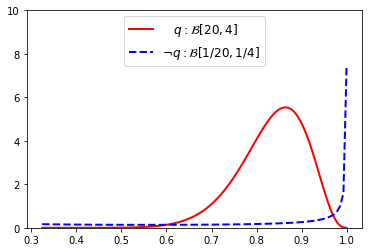
Figure 4: Illustration of an example where the negation operator of BetaE does not satisfy non-contradiction, i.e. $\phi(\neg q,e)$ is not monotonically decreasing with regard to $\phi(q,e)$.

Appendix D Dataset statistics and query structures

We use the benchmark datasets provided by BetaE (Ren and Leskovec 2020), which is publicly available at https://github.com/snap-stanford/KGReasoning. The datasets contain 14 types of logical queries on FB15k-237 (Toutanova and Chen 2015) and NELL995 (Xiong, Hoang, and Wang 2017) respectively. The queries are generated based on the official training/validation/testing edge splits of those KGs. The 14 types of query structures in the datasets are shown in Fig. 3. We list the number of training/validation/test queries in Table 8. The KG statistics are summarized in Table 7.

Table 7: Knowledge graph dataset statistics as well as training, validation, and test edge splits.

Dataset	Entities	Relations	Training Edges	Validation Edges	Test Edges	Total Edges
FB15k-237	14505	237	272115	17526	20438	310079
NELL	63361	200	114213	143234	14267	142804

Table 8: Number of training, validation, and test queries for different query structures. For columns that list multiple query structures, the number in the table represents the number of each query structure.

	Training		Validation		Test
Dataset	1p/2p/3p/2i/3i	2in/3in/inp/pin/pni	1p	others	1p	others
FB15k-237	149,689	149,68	20,101	5,000	2,812	5,000
NELL995	107,982	10,798	16,927	4,000	17,034	4,000

Appendix E Experimental details

Implementation

For GQE (Hamilton et al. 2018), Query2Box (Ren, Hu, and Leskovec 2020), and BetaE (Ren and Leskovec 2020), we use the implementation from https://github.com/snap-stanford/KGReasoning. For CQD, we use the implementation at https://github.com/uclnlp/cqd. The source code of our model is included in a code appendix. All source code of our model will be made publicly available upon publication of the paper with a license that allows free usage for research purposes.

Model configurations and hyperparameters

We use AdamW (Loshchilov and Hutter 2019) as the optimizer. Training terminates with early stopping based on the average MRR on the validation set with a patience of 15k steps. We run each method up to 450k steps. We repeat each experiment three times and report the average results.

As in (Ren, Hu, and Leskovec 2020; Ren and Leskovec 2020), for fair comparison, we use the same embedding dimensionality $d$ and the number of negative samples $k$ for all the methods. With reference to (Ren and Leskovec 2020), we set the embdding dimensionality to $d=800$ and use $k=128$ negative samples per positive sample. We finetune other hyperparameters and the choice of the subspace mapping function $\mathbf{g}:\mathbb{R}^{d}\rightarrow[0,1]^{d}$ by grid search based on the average MRR on the validation set. We search hyperparameters in the following range: learning rate from $\{0.001,0.0005,0.0001\}$, number of relation bases from $\{30,50,100,150\}$, batch size $b$ from {128, 512, 1000}. $\mathbf{g}$ is chosen from from {Logistic function, Bounded rectifier}.

The best hyperparameter combination on FB15k-237 is learning rate $0.001$, number of relation bases $150$, batch size $512$, $\mathbf{g}$ as a logistic function. The best combination on NELL995 is learning rate $0.0005$, number of relation bases $30$, batch size $1000$, $\mathbf{g}$ as a bounded rectifier. For baselines GQE , Q2B, and BetaE, we use the best combinations reported by (Ren and Leskovec 2020). For CQD, we use the ones reported in (Arakelyan et al. 2021). We follow the setting in the official code repository for any hyperparameter unspecified in the paper.

Hardware and software Specifications

Each single experiment is run on CPU $\text{Intel}^{\circledR}$ $\text{Xeon}^{\circledR}$ E5-2650 v4 12-core and a single $\text{NVIDIA}^{\circledR}$ GP102 TITAN Xp (12GB) GPU. RAM size is 256GB. The operating system is Ubuntu 18.04.01. Our framework is implemented wtih Python 3.9 and Pytorch 1.9.

Appendix F $t$-norm based fuzzy logic systems

Functions that qualify as fuzzy conjunction and fuzzy disjunction are usually referred to in literature as $t$-norms  (triangular norms) and $t$-conorms  (triangular conorms) respectively in literature (Klir and Yuan 1995).

A $t$-norm (Dubois and Prade 1980) is a function $t:[0,1]\times[0,1]\rightarrow[0,1]$ which is commutative and associative and satisfies the boundary condition $t(a,1)=a$ as well as monotonicity, i.e., $t(a,b)\leq t(c,d)$ if $a\leq c$ and $b\leq d$. Prominent examples of $t$-norms include minimum, product, and Łukasiewicz $t$-norm.

$t$-conorm is the logical dual form of the $t$-norm. Following De Morgan's law, given the canonical negator $c(x)=1-x$, the $t$-conorm  $s$ of a $t$-norm $t$ is defined as $s(a,b)=1-t(1-a,1-b)$. A $t$-conorm is commutative and associative, and satisfies the boundary condition $s(a,0)=a$ as well as monotonicity: $s(a,b)\leq s(c,d)$ if $a\leq c$ and $b\leq d$. Interested readers are referred to (Klir and Yuan 1995) for proofs.

The formulas of $t$-conorms that correspond to the minimum (Gödel), product, and Łukasiewicz $t$-norms are given in Table 9. The illustration is given in Fig 5.

Table 9: Prominent examples of $t$-norms and the corresponding $t$-norms derived by De Morgan's law and the canonical negator $c(x)=1-x$. We list the special properties of the formulas in addition to the basic properties (i.e., commutativity, associativity, monotonicity, and boundary condition) of t-norm and t-conorm.

$t$-norm ($\land$)		$t$-conorm ($\lor$)	Special Properties
minimum (Gödel)	$t(a,b)=\min(a,b)$	$s(a,b)=\max(a,b)$	idempotent
product	$t(a,b)=ab$	$s(a,b)=a+b-ab$	strict monotonicity
Łukasiewicz	$t(a,b)=\max(a+b-1,0)$	$s(a,b)=\min(a+b,1)$	nilpotent

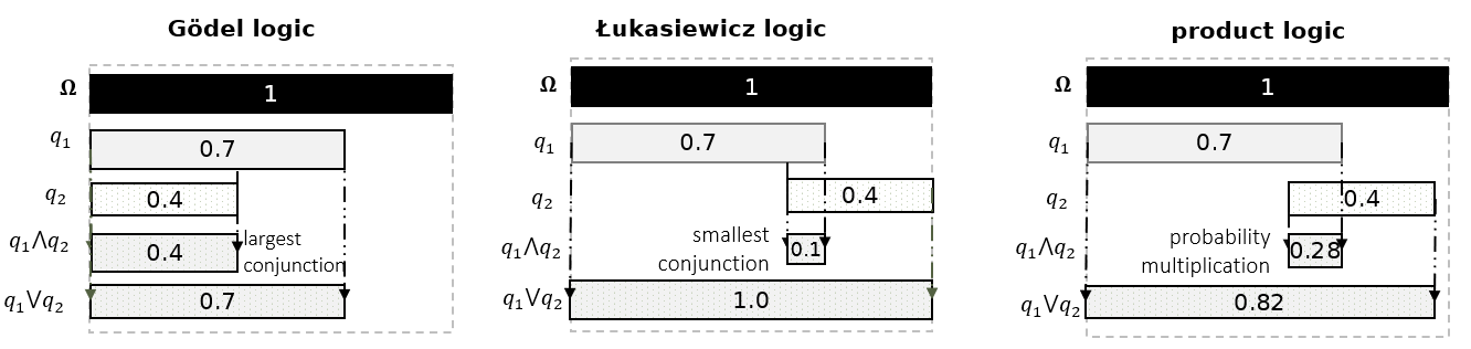
Figure 5: Illustration of fuzzy conjunction and disjunction, which is equivalent to fuzzy set intersection and union.

Appendix G Time Comparison with CQD

We compare with CQD with regard to the time for answering a query. The experiment is conducted on a $\text{NVIDIA}^{\circledR}$ GP102 TITAN Xp (12GB) GPU. The full hardware and software specifications are given in Appendix E. For CQD, we use its official implementation and experiment setting (Arakelyan et al. 2021). The beam search candidate number for CQD is set as $64$, i.e., CQD finds top $64$ entity candidates for each sub-query and uses it as seeds for search in the next round. For FuzzQE, we retrieve top $64$ entity candidates for each query as well. We use FAISS (Johnson, Douze, and Jégou 2017) to speed up dense similarity search, whereexact measurement matching is adopted instead of approximate measurement matching. FAISS cannot be applied to CQD, because (i) CQD is not a logical query embedding framework that retrieves entity answers by dense similarity search, and (ii) scoring an entity for a query involves computation in the complex number domain.

Fig 6 shows the average time of CQD and FuzzQE for answering a complex FOL query. Fig 7 shows the time required by CQD and FuzzQE for answering each query type, aggregated over FB15k-237 and NELL995. The structure of different query types are shown in Fig. 3 in Appendix D. Consistent with the observation in (Arakelyan et al. 2021), the main computation bottleneck of CQD are multi-hop queries (e.g., $3p$ queries), since the model is required to invoke the link prediction model for each node in the dependency graph to obtain the top-$k$ candidates for the next step. We also note that as the number of entities increases, the time required by CQD to answer a query significantly grows. In contrast, the inference time of FuzzQE is almost independent of the number of entities and the complexity of the query.

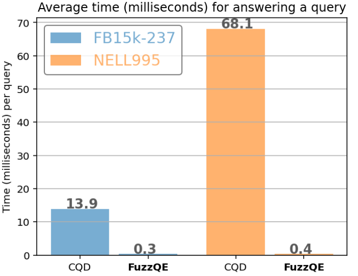
Figure 6: Average time (milliseconds) for answering an FOL query on a single $\text{NVIDIA}^{\circledR}$ GP102 TITAN Xp (12GB) GPU. FB15k-237 contains 14,505 entities. NELL995 contains 63,361 entities, roughly 4 times the number of FB15k-237.

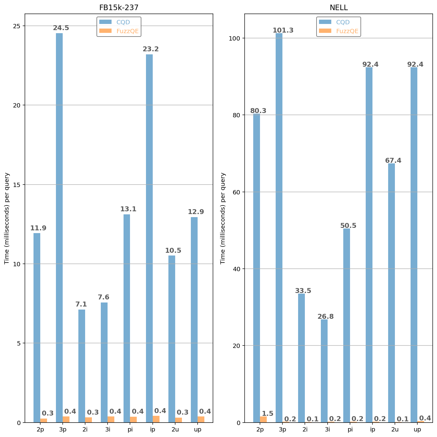
Figure 7: Average time (milliseconds) required by CQD and FuzzQE for answering each query type in FB15k-237 and NELL995.

References

- Arakelyan et al. (2021) Arakelyan, E.; Daza, D.; Minervini, P.; and Cochez, M. 2021. Complex Query Answering with Neural Link Predictors. In 9th International Conference on Learning Representations, ICLR 2021, Virtual Event, Austria, May 3-7, 2021. OpenReview.net.
- Ba, Kiros, and Hinton (2016) Ba, L. J.; Kiros, J. R.; and Hinton, G. E. 2016. Layer Normalization. CoRR, abs/1607.06450.
- Balaraman, Razniewski, and Nutt (2018) Balaraman, V.; Razniewski, S.; and Nutt, W. 2018. Recoin: Relative Completeness in Wikidata. In Companion Proceedings of the The Web Conference 2018, WWW '18, 1787–1792. Republic and Canton of Geneva, CHE: International World Wide Web Conferences Steering Committee. ISBN 9781450356404.
- Bollacker et al. (2008) Bollacker, K.; Evans, C.; Paritosh, P.; Sturge, T.; and Taylor, J. 2008. Freebase: a collaboratively created graph database for structuring human knowledge. In Proceedings of ACM SIGMOD International Conference on Management of Data (SIGMOD).
- Bordes et al. (2013) Bordes, A.; Usunier, N.; Garcia-Duran, A.; Weston, J.; and Yakhnenko, O. 2013. Translating embeddings for modeling multi-relational data. In Advances in Neural Information Processing Systems (NIPS), 2787–2795.
- Chvalovskỳ (2012) Chvalovskỳ, K. 2012. On the independence of axioms in BL and MTL. Fuzzy Sets and Systems, 197: 123–129.
- Cormode and Muthukrishnan (2005) Cormode, G.; and Muthukrishnan, S. 2005. An improved data stream summary: the count-min sketch and its applications. J. Algorithms, 55(1): 58–75.
- Dubois and Prade (1980) Dubois, D.; and Prade, H. 1980. Systems of linear fuzzy constraints. Fuzzy sets and systems, 3(1): 37–48.
- Fodor and Roubens (1994) Fodor, J. C.; and Roubens, M. 1994. Fuzzy Preference Modelling and Multicriteria Decision Support, volume 14 of Theory and Decision Library. Springer. ISBN 978-90-481-4466-2.
- Friedman and Van den Broeck (2020) Friedman, T.; and Van den Broeck, G. 2020. Symbolic Querying of Vector Spaces: Probabilistic Databases Meets Relational Embeddings. In Adams, R. P.; and Gogate, V., eds., Proceedings of the Thirty-Sixth Conference on Uncertainty in Artificial Intelligence, UAI 2020, virtual online, August 3-6, 2020, volume 124 of Proceedings of Machine Learning Research, 1268–1277. AUAI Press.
- Guu, Miller, and Liang (2015) Guu, K.; Miller, J.; and Liang, P. 2015. Traversing Knowledge Graphs in Vector Space. In Màrquez, L.; Callison-Burch, C.; Su, J.; Pighin, D.; and Marton, Y., eds., Proceedings of the 2015 Conference on Empirical Methods in Natural Language Processing, EMNLP 2015, Lisbon, Portugal, September 17-21, 2015, 318–327. The Association for Computational Linguistics.
- Hamilton et al. (2018) Hamilton, W. L.; Bajaj, P.; Zitnik, M.; Jurafsky, D.; and Leskovec, J. 2018. Embedding Logical Queries on Knowledge Graphs. In Advances in Neural Information Processing Systems 31: Annual Conference on Neural Information Processing Systems 2018, NeurIPS 2018, December 3-8, 2018, Montréal, Canada, 2030–2041.
- Hartig and Heese (2007) Hartig, O.; and Heese, R. 2007. The SPARQL query graph model for query optimization. In European Semantic Web Conference, 564–578. Springer.
- Ji et al. (2015) Ji, G.; He, S.; Xu, L.; Liu, K.; and Zhao, J. 2015. Knowledge graph embedding via dynamic mapping matrix. In Proceedings of the Annual Meeting of Associations for Computational Linguistics (ACL), 687–696. The Association for Computer Linguistics.
- Johnson, Douze, and Jégou (2017) Johnson, J.; Douze, M.; and Jégou, H. 2017. Billion-scale similarity search with GPUs. arXiv preprint arXiv:1702.08734.
- Katsaras and Liu (1977) Katsaras, A.; and Liu, D. 1977. Fuzzy vector spaces and fuzzy topological vector spaces. Journal of Mathematical Analysis and Applications, 58(1): 135–146.
- Klement, Mesiar, and Pap (2000) Klement, E.; Mesiar, R.; and Pap, E. 2000. Triangular Norms, volume 8 of Trends in Logic. Springer. ISBN 978-90-481-5507-1.
- Klir and Yuan (1995) Klir, G.; and Yuan, B. 1995. Fuzzy sets and fuzzy logic, volume 4. Prentice hall New Jersey.
- Loshchilov and Hutter (2019) Loshchilov, I.; and Hutter, F. 2019. Decoupled Weight Decay Regularization. In 7th International Conference on Learning Representations, ICLR 2019, New Orleans, LA, USA, May 6-9, 2019. OpenReview.net.
- Mitchell et al. (2018) Mitchell, T.; Cohen, W.; Hruschka, E.; Talukdar, P.; Yang, B.; Betteridge, J.; Carlson, A.; Dalvi, B.; Gardner, M.; Kisiel, B.; et al. 2018. Never-ending learning. Communications of the ACM.
- Rebele et al. (2016) Rebele, T.; Suchanek, F.; Hoffart, J.; Biega, J.; Kuzey, E.; and Weikum, G. 2016. YAGO: A multilingual knowledge base from wikipedia, wordnet, and geonames. In Proceedings of the International Semantic Web Conference (ISWC), volume 9982 of Lecture Notes in Computer Science, 177–185. Springer.
- Ren, Hu, and Leskovec (2020) Ren, H.; Hu, W.; and Leskovec, J. 2020. Query2box: Reasoning over Knowledge Graphs in Vector Space Using Box Embeddings. In 8th International Conference on Learning Representations, ICLR 2020, Addis Ababa, Ethiopia, April 26-30, 2020. OpenReview.net.
- Ren and Leskovec (2020) Ren, H.; and Leskovec, J. 2020. Beta Embeddings for Multi-Hop Logical Reasoning in Knowledge Graphs. In Advances in Neural Information Processing Systems 33: Annual Conference on Neural Information Processing Systems 2020, NeurIPS 2020, December 6-12, 2020, virtual.
- Schlichtkrull et al. (2018) Schlichtkrull, M. S.; Kipf, T. N.; Bloem, P.; van den Berg, R.; Titov, I.; and Welling, M. 2018. Modeling Relational Data with Graph Convolutional Networks. In The Semantic Web - 15th International Conference, ESWC 2018, Heraklion, Crete, Greece, June 3-7, 2018, Proceedings, volume 10843 of Lecture Notes in Computer Science, 593–607. Springer.
- Schmidt, Meier, and Lausen (2010) Schmidt, M.; Meier, M.; and Lausen, G. 2010. Foundations of SPARQL query optimization. In Proceedings of the 13th International Conference on Database Theory, 4–33.
- Shrivastava and Li (2014) Shrivastava, A.; and Li, P. 2014. Asymmetric LSH (ALSH) for Sublinear Time Maximum Inner Product Search (MIPS). In Ghahramani, Z.; Welling, M.; Cortes, C.; Lawrence, N. D.; and Weinberger, K. Q., eds., Advances in Neural Information Processing Systems 27: Annual Conference on Neural Information Processing Systems 2014, December 8-13 2014, Montreal, Quebec, Canada, 2321–2329.
- Sun et al. (2020) Sun, H.; Arnold, A. O.; Bedrax-Weiss, T.; Pereira, F.; and Cohen, W. W. 2020. Faithful Embeddings for Knowledge Base Queries. In Larochelle, H.; Ranzato, M.; Hadsell, R.; Balcan, M.; and Lin, H., eds., Advances in Neural Information Processing Systems 33: Annual Conference on Neural Information Processing Systems 2020, NeurIPS 2020, December 6-12, 2020, virtual.
- Sun et al. (2019) Sun, Z.; Deng, Z.-H.; Nie, J.-Y.; and Tang, J. 2019. RotatE: Knowledge graph embedding by relational rotation in complex space. In International Conference on Learning Representations (ICLR).
- Toutanova and Chen (2015) Toutanova, K.; and Chen, D. 2015. Observed versus latent features for knowledge base and text inference. In Proceedings of the 3rd workshop on continuous vector space models and their compositionality, 57–66.
- Trouillon et al. (2016) Trouillon, T.; Welbl, J.; Riedel, S.; Gaussier, E.; and Bouchard, G. 2016. Complex embeddings for simple link prediction. In Proceedings of the International Conference on Machine Learning (ICML), volume 48, 2071–2080. PMLR.
- Vrandečić and Krötzsch (2014) Vrandečić, D.; and Krötzsch, M. 2014. Wikidata: a free collaborative knowledge base. Communications of ACM, 57(10): 78–85.
- Xiong, Hoang, and Wang (2017) Xiong, W.; Hoang, T.; and Wang, W. Y. 2017. DeepPath: A Reinforcement Learning Method for Knowledge Graph Reasoning. In Palmer, M.; Hwa, R.; and Riedel, S., eds., Proceedings of the 2017 Conference on Empirical Methods in Natural Language Processing, EMNLP 2017, Copenhagen, Denmark, September 9-11, 2017, 564–573. Association for Computational Linguistics.
- Yang et al. (2015) Yang, B.; Yih, W.-t.; He, X.; Gao, J.; and Deng, L. 2015. Embedding entities and relations for learning and inference in knowledge bases. International Conference on Learning Representations (ICLR).
- Zaheer et al. (2017) Zaheer, M.; Kottur, S.; Ravanbakhsh, S.; Póczos, B.; Salakhutdinov, R.; and Smola, A. J. 2017. Deep Sets. In Guyon, I.; von Luxburg, U.; Bengio, S.; Wallach, H. M.; Fergus, R.; Vishwanathan, S. V. N.; and Garnett, R., eds., Advances in Neural Information Processing Systems 30: Annual Conference on Neural Information Processing Systems 2017, December 4-9, 2017, Long Beach, CA, USA, 3391–3401.
- Zimmermann (1991) Zimmermann, H. 1991. Fuzzy Set Theory - and Its Applications. Springer. ISBN 978-94-015-7951-3.
- Zou et al. (2011) Zou, L.; Mo, J.; Chen, L.; Özsu, M. T.; and Zhao, D. 2011. GStore: Answering SPARQL Queries via Subgraph Matching. Proc. VLDB Endow., 4(8): 482–493.