Geometry of skew information-based quantum coherence

Abstract We study the skew information-based coherence of quantum states and derive explicit formulas for Werner states and isotropic states in a set of autotensor of mutually unbiased bases (AMUBs). We also give surfaces of skew information-based coherence for Bell-diagonal states and a special class of $X$ states in both computational basis and in mutually unbiased bases. Moreover, we depict the surfaces of the skew information-based coherence for Bell-diagonal states under various types of local nondissipative quantum channels. The results show similar as well as different features compared with relative entropy of coherence and $l_{1}$ norm of coherence.

Key Words coherence; skew information; mutually unbiased bases; quantum channels

PACS numbers 03.67.-a, 03.65.Ta

1. Introduction

Quantum coherence is an intrinsic character of quantum mechanics which plays significant roles in superconductivity, quantum thermodynamics and biological processes, while a theoretic framework to quantify the coherence was not formulated until the work of [1]. It intrigued great interest in studying quantum coherence from different perspectives and aspects.

A large number of valid coherence measures or coherence monotones such as relative entropy of coherence, $l_{1}$ norm of coherence, robustness of coherence, coherence of formation, max-relative entropy of coherence, modified trace distance of coherence, skew information-based coherence, geometric coherence, coherence weight, affinity distance-based coherence, generalized $\alpha$-$z$-relative Rényi entropy of coherence and various entropic-based coherence measures have been proposed to quantify quantum coherence [1, 2, 3, 4, 5, 6, 7, 8, 9, 10, 11, 12, 13, 14, 15, 16]. Average coherence and coherence-generating power of quantum channels based on different coherence measures have also been extensively explored [17, 18, 19, 20, 21, 22, 23, 24, 25, 26]. Moreover, the interconversion between quantum coherence and quantum entanglement or quantum correlations are formulated [27, 28, 29, 30, 31, 32, 33, 34].

On the other hand, the problem of coherence distillation and coherence dilution have also been discussed [35, 36, 37, 38, 39, 40, 41, 42], together with the no-broadcasting of quantum coherence [43, 44]. A complete theory of one-shot coherence distillation has been formulated in [45]. Quantum coherence can also be used to certify quantum memories [46]. The quantum coherence among nondegenerate energy subspaces (CANES) has been shown to be essential for the energy flow in any quantum system [47].

The concept of mutually unbiased bases (MUBs) was raised in quantum state determinations. It is found to be possible to construct $d+1$ MUBs of the space $\mathbb{C}^{d}$ if $d$ is a prime power, i.e., $d=p^{n}$, where $p$ is a prime number and $n$ is an integer [48, 49]. It is still not known yet that what are the maximal sets of MUBs when the dimension $d$ is a composite number [50]. The link between unextendible maximally entangled bases and mutually unbiased bases has been established [51], and entanglement, compatibility of measurements and uncertainty relations with respect to MUBs have been investigated [52, 53, 54, 55, 56].

The geometry of entanglement measures and other correlation measures can provide an intuition towards the quantification of these correlations. The level surfaces of entanglement and quantum discord for Bell-diagonal states [57], the level surfaces of quantum discord for a class of two-qubit states [58], the geometry of one-way information deficit for a class of two-qubit states [59], the surfaces of constant quantum discord and super-quantum discord for Bell-diagonal states [60] have been depicted. Recently, the $l_{1}$ norm of coherence of quantum states in mutually unbiased bases has been discussed [61], and the geometry with respect to relative entropy of coherence and $l_{1}$ norm of coherence for Bell-diagonal states has been investigated [62, 63].

In this paper, we calculate skew information-based coherence of quantum states in mutually unbiased bases for qubit and two-qubit quantum states, and formulate the corresponding geometries. We explore the geometry of skew information-based coherence of two-qubit Bell-diagonal states and $X$ states in both computational basis and in mutually unbiased bases. We also investigate the dynamic behavior of the skew information-based coherence under different quantum channels.

2. Skew information-based coherence in autotensor of mutually unbiased bases

Let $\mathcal{H}$ be a $d$-dimensional Hilbert space, and $\mathcal{B(H)}$, $\mathcal{S(H)}$ and $\mathcal{D(H)}$ be the set of all bounded linear operators, Hermitian operators and density operators on $\mathcal{H}$, respectively. Usually, a state and a channel are mathematically described by a density operator (positive operator of trace $1$) and a completely positive trace preserving (CPTP) map, respectively [64].

The set of incoherent states, which are diagonal matrices in the fixed orthonormal base $\{|k\rangle\}^{d}_{k=1}$ of the $d$-dimensional Hilbert space $\mathcal{H}$, can be represented as

$$\mathcal{I}=\{\delta\in\mathcal{D(H)}|\delta=\sum_{i}p_{i}|i\rangle\langle i|,~{}p_{i}\geq 0,~{}\sum_{i}p_{i}=1\}.$$

Let $\Lambda$ be a CPTP map $\Lambda(\rho)=\sum_{n}K_{n}\rho K_{n}^{\dagger},$ where $K_{n}$ are Kraus operators satisfying $\sum_{n}K_{n}^{\dagger}K_{n}=I_{d}$ with $I_{d}$ the identity operator. $K_{n}$ are called incoherent Kraus operators if $K_{n}^{\dagger}\mathcal{I}K_{n}\in\mathcal{I}$ for all $n$, and the corresponding $\Lambda$ is called an incoherent operation.

A well-defined coherence measure $C(\rho)$ shall satisfy the following conditions [1]:

$(C1)$ (Faithfulness) $C(\rho)\geq 0$ and $C(\rho)=0$ iff $\rho$ is incoherent.

$(C2)$ (Convexity) $C(\cdot)$ is convex in $\rho$.

$(C3)$ (Monotonicity) $C(\Lambda(\rho))\leq C(\rho)$ for any incoherent operation $\Lambda$.

$(C4)$ (Strong monotonicity) $C(\cdot)$ does not increase on average under selective incoherent operations, i.e.,

$$C(\rho)\geq\sum_{n}p_{n}C(\varrho_{n}),$$

where $p_{n}=\mathrm{Tr}(K_{n}\rho K_{n}^{\dagger})$ are probabilities and $\varrho_{n}=\frac{K_{n}\rho K_{n}^{\dagger}}{p_{n}}$ are the post-measurement states, $K_{n}$ are incoherent Kraus operators.

For a state $\rho\in\mathcal{D(H)}$ and an observable $K\in\mathcal{S(H)}$, the Wigner-Yanase (WY) skew information is defined by [65]

$$I(\rho,K)=-\frac{1}{2}\mathrm{Tr}([\rho^{\frac{1}{2}},K]^{2}),$$ (1)

where $[X,Y]:=XY-YX$ is the commutator of $X$ and $Y$.

In an attempt to quantify coherence [66], Girolami proposed to use the Wigner-Yanase skew information $I(\rho,K)$ to quantify coherence, and called it $K$-coherence. Here $K$ is diagonal in the base $\{|k\rangle\}_{k=1}^{d}$. More precisely, this quantity should be considered as a quantifier for coherence of $\rho$ with respect to the observable $K$ rather than the associated orthonormal base.

The absence of a reference frame has been proven equivalent to constrain quantum dynamics by a superselection rule (SSR) [67], while the ability of a system to act as reference frame is the quantum resource known as asymmetry or frameness [67]. A $G$-SSR for a quantity $Q$ (supercharge) is defined as a law of invariance of the state of a system with respect to a transformation group $G$. In [66], it is shown that given a $G$-SSR with supercharge $Q$, the skew information $I(\rho,Q)=-\frac{1}{2}\mathrm{Tr}([\rho^{\frac{1}{2}},Q]^{2})$ satisfies the criteria identifying an asymmetry measure of the state [68]. It is worth noting that quantum asymmetry represents the amount of coherence in the eigenbasis of the supercharge [68].

The $K$-coherence satisfies $(C1)$ and $(C2)$, but not $(C3)$, as pointed out in [69, 70]. By using the spectral decomposition of the observable $K$ rather than the observable $K$ itself, the authors in [10] have showed that the $K$-coherence can be simply modified to be a bona fide measure of coherence satisfying the above requirements $(C1)$-$(C3)$ (where they called it partial coherence).

Another way to solve the problem is proposed in [8] by introducing the skew information-based coherence measure defined by [8]

$$C_{I}(\rho)=\sum_{k=1}^{d}I(\rho,|k\rangle\langle k|),$$ (2)

where $I(\rho,|k\rangle\langle k|)=-\frac{1}{2}\mathrm{Tr}\{[\rho,|k\rangle\langle k|]\}^{2}$ is the skew information of the state $\rho$ with respect to the projections $\{|k\rangle\langle k|\}_{k=1}^{d}$. Direct calculation shows that the coherence measure (2) can be written as

$$C_{I}(\rho)=1-\sum_{k=1}^{d}\langle k|\sqrt{\rho}|k\rangle^{2}.$$ (3)

In [8], it has been proved that the coherence measure defined in (2) satisfies all the criteria $(C1)$-$(C4)$, while the $K$-coherence does not satisfy $(C4)$ (strong monotonicity). The coherence measure has an analytic expression and an obvious operational meaning related to quantum metrology. In terms of this coherence measure, the distribution of the quantum coherence among the multipartite systems has been studied and a corresponding polygamy relation has been proposed. It is also found that the coherence measure gives the natural upper bounds of quantum correlations prepared by incoherent operations. Moreover, it is shown that this coherence measure can be experimentally measured. Since the skew information-based coherence measure (2) is of great significance both theoretically and practically, it is worth evaluating the measure for classes of quantum states in both computational basis and mutually unbiased bases, and studying the geometrical characters.

A set of orthonormal bases $\{e_{k}\}=\{|0\rangle_{k},|1\rangle_{k},\cdots,|d-1\rangle_{k}\}$ for a Hilbert space $H=\mathbb{C}^{d}$ is called MUBs if [48, 49]

$$|_{k}\langle i|j\rangle_{l}|=\frac{1}{\sqrt{d}}$$

holds for all $i,j\in\{0,1,\cdots,d-1\}$ and $k\neq l$. For $d=2$, a set of three mutually unbiased bases is given by

$$e_{1}=\{e_{11},e_{12}\}=\{|0\rangle,|1\rangle\},$$

$$e_{2}=\{e_{21},e_{22}\}=\left\{\frac{1}{\sqrt{2}}(|0\rangle+|1\rangle),\frac{1}{\sqrt{2}}(|0\rangle-|1\rangle)\right\},$$

$$e_{3}=\{e_{31},e_{32}\}=\left\{\frac{1}{\sqrt{2}}(|0\rangle+i|1\rangle),\frac{1}{\sqrt{2}}(|0\rangle-i|1\rangle)\right\}.$$

Let $\{e_{k}\}=\{|0\rangle_{k},|1\rangle_{k},\cdots,|d-1\rangle_{k}\}$ be a set of mutually unbiased bases. The set $\{a_{k}\}=\{|i\rangle_{k}\otimes|j\rangle_{k},i,j=0,1,\cdots,d-1\}$ is called the autotensor of mutually unbiased bases (AMUBs) if [61]

$$|(\langle i|_{k}\otimes\langle j|_{k})(|m\rangle_{l}\otimes|n\rangle_{l})|=\frac{1}{d},~{}~{}~{}i,j,m,n=0,...,d-1,$$

for $k\neq l$. The following set is an AMUBs derived from two-dimensional MUBs [61]:

$$\{a_{1}\}=\{a_{11},a_{12},a_{13},a_{14}\}=\{e_{11}\otimes e_{11},e_{11}\otimes e_{12},e_{12}\otimes e_{11},e_{12}\otimes e_{12}\},$$

$$\{a_{2}\}=\{a_{21},a_{22},a_{23},a_{24}\}=\{e_{21}\otimes e_{21},e_{21}\otimes e_{22},e_{22}\otimes e_{21},e_{22}\otimes e_{22}\},$$

$$\{a_{3}\}=\{a_{31},a_{32},a_{33},a_{34}\}=\{e_{31}\otimes e_{31},e_{31}\otimes e_{32},e_{32}\otimes e_{31},e_{32}\otimes e_{32}\}.$$

In general, a two qubit $X$ states can be represented as

$$\rho^{X}=\frac{1}{4}(I\otimes I+\mathbf{r}\cdot\sigma\otimes I+I\otimes\mathbf{s}\cdot\sigma+\sum_{i=1}^{3}c_{i}\sigma_{i}\otimes\sigma_{i}),$$ (4)

where $\mathbf{r}$ and $\mathbf{s}$ are Bloch vectors. As a special class of $\rho^{X}$, for $\mathbf{r}=\mathbf{s}=0$, one obtains the two-qubit Bell-diagonal states

$$\rho^{BD}=\frac{1}{4}\left(I\otimes I+\sum_{i=1}^{3}c_{i}\sigma_{i}\otimes\sigma_{i}\right),$$ (5)

where $c_{i}\in[-1,1]$, $i=1,2,3$.

The density matrix of $\rho^{BD}$ in basis $a_{1}$ is of the form

$$(\rho^{BD})_{a_{1}}=\frac{1}{4}\left(\begin{array}[]{cccc}1+c_{3}&0&0&c_{1}-c_{2}\\ 0&1-c_{3}&c_{1}+c_{2}&0\\ 0&c_{1}+c_{2}&1-c_{3}&0\\ c_{1}-c_{2}&0&0&1+c_{3}\\ \end{array}\right),$$

and the skew information-based coherence of $(\rho^{BD})_{a_{1}}$ is

$$C_{I}(\rho^{BD})_{a_{1}}=\frac{1}{4}(2-\sqrt{1-c_{1}-c_{2}-c_{3}}\sqrt{1+c_{1}+c_{2}-c_{3}}-\sqrt{1+c_{1}-c_{2}+c_{3}}\sqrt{1-c_{1}+c_{2}+c_{3}}).$$ (6)

Similarly, the density matrix of $\rho^{BD}$ in basis $a_{2}$ and $a_{3}$ are given by

$$(\rho^{BD})_{a_{2}}=\frac{1}{4}\left(\begin{array}[]{cccc}1+c_{1}&0&0&c_{3}-c_{2}\\ 0&1-c_{1}&c_{3}+c_{2}&0\\ 0&c_{3}+c_{2}&1-c_{1}&0\\ c_{3}-c_{2}&0&0&1+c_{1}\\ \end{array}\right)$$

and

$$(\rho^{BD})_{a_{3}}=\frac{1}{4}\left(\begin{array}[]{cccc}1+c_{2}&0&0&c_{3}-c_{1}\\ 0&1-c_{2}&c_{3}+c_{1}&0\\ 0&c_{3}+c_{1}&1-c_{2}&0\\ c_{3}-c_{1}&0&0&1+c_{2}\\ \end{array}\right),$$

with the skew information-based coherence

$$C_{I}(\rho^{BD})_{a_{2}}=\frac{1}{4}(2-\sqrt{1+c_{1}+c_{2}-c_{3}}\sqrt{1+c_{1}-c_{2}+c_{3}}-\sqrt{1-c_{1}-c_{2}-c_{3}}\sqrt{1-c_{1}+c_{2}+c_{3}})$$ (7)

and

$$C_{I}(\rho^{BD})_{a_{3}}=\frac{1}{4}(2-\sqrt{1-c_{1}-c_{2}-c_{3}}\sqrt{1+c_{1}-c_{2}+c_{3}}-\sqrt{1+c_{1}+c_{2}-c_{3}}\sqrt{1-c_{1}+c_{2}+c_{3}}),$$ (8)

respectively. We plot the level surfaces of $C_{I}(\rho^{BD})_{a_{1}}$ in Figure 1.

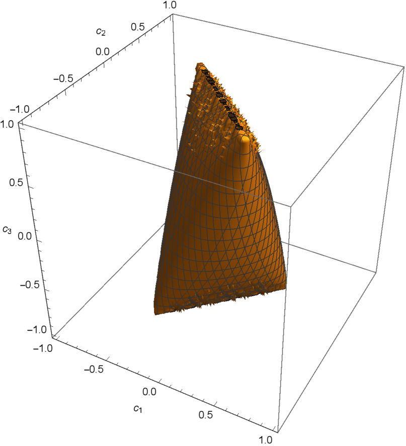
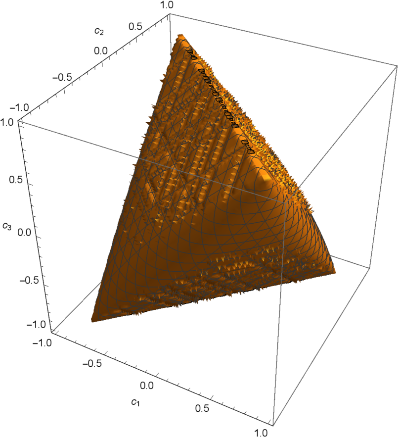
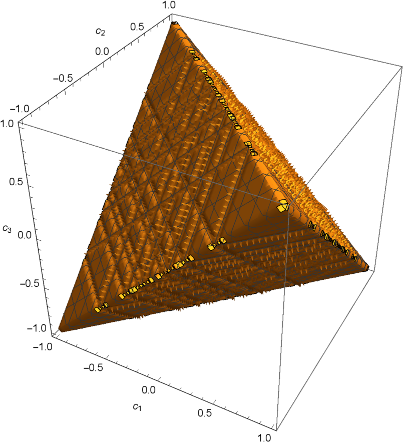
Figure 1: Surfaces of constant $C_{I}(\rho^{BD})_{a_{1}}$: (a) $C_{I}(\rho^{BD})_{a_{1}}=0.05$; (b) $C_{I}(\rho^{BD})_{a_{1}}=0.2$; (c) $C_{I}(\rho^{BD})_{a_{1}}=1$.

The Bell-diagonal state $\rho^{BD}$ becomes the Werner state $\rho^{W}$ if we take $c_{1}=c_{2}=c_{3}=\frac{3}{4}p-1$ ($0\leq p\leq 1$). We have

$$(\rho^{W})_{a_{i}}=\left(\begin{array}[]{cccc}\frac{1}{3}p&0&0&0\\ 0&\frac{1}{6}(3-2p)&\frac{1}{6}(4p-3)&0\\ 0&\frac{1}{6}(4p-3)&\frac{1}{6}(3-2p)&0\\ 0&0&0&\frac{1}{3}p\\ \end{array}\right),~{}~{}~{}i=1,2,3,$$

and

$$C_{I}(\rho^{W})_{a_{i}}=\frac{1}{16}(8-\sqrt{p(48-27p)}-3p),~{}~{}~{}i=1,2,3.$$ (9)

Taking $c_{1}=c_{3}=\frac{4F-1}{3}$, $c_{2}=-\frac{4F-1}{3}$ ($0\leq F\leq 1$), we have the isotropic state $\rho^{iso}$,

$$(\rho^{iso})_{a_{i}}=\left(\begin{array}[]{cccc}\frac{1}{6}(1+2F)&0&0&\frac{1}{6}(4F-1)\\ 0&\frac{1}{3}(1-F)&0&0\\ 0&0&\frac{1}{3}(1-F)&0\\ \frac{1}{6}(4F-1)&0&0&\frac{1}{6}(1+2F)\\ \end{array}\right),~{}~{}~{}i=1,2,$$

and

$$(\rho^{iso})_{a_{3}}=\left(\begin{array}[]{cccc}\frac{1}{3}(1-F)&0&0&0\\ 0&\frac{1}{6}(1+2F)&0&0\\ 0&0&\frac{1}{6}(1+2F)&0\\ 0&0&0&\frac{1}{3}(1-F)\\ \end{array}\right),$$

from which we obtain

$$C_{I}(\rho^{iso})_{a_{i}}=\frac{1}{6}(1+2F-2\sqrt{3F(1-F)}),~{}~{}~{}i=1,2,3.$$ (10)

The $C$-axis stands for $C_{I}(\rho^{W})_{a_{i}}$ and $C_{I}(\rho^{iso})_{a_{i}}(i=1,2,3)$ in Figure 2(a) and (b), respectively.

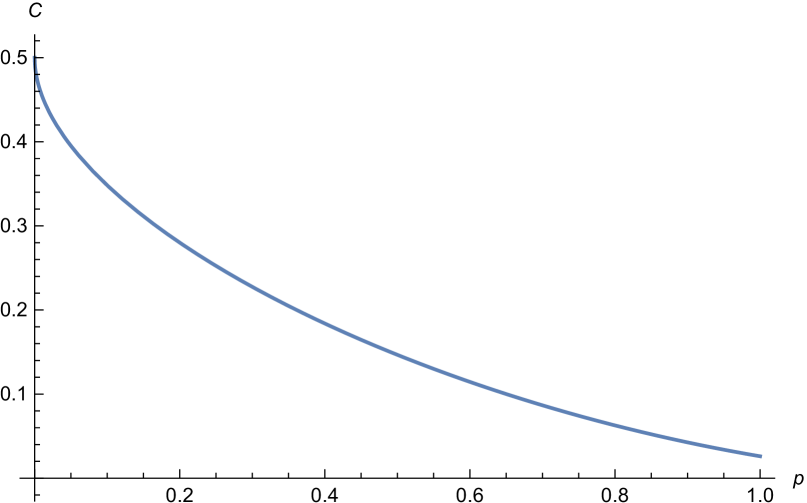
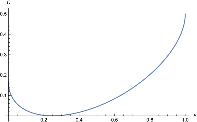
Figure 2: (a) $C_{I}(\rho^{W})_{a_{i}}(i=1,2,3)$ as a function of $p$; (b) $C_{I}(\rho^{iso})_{a_{i}}(i=1,2,3)$ as a function of $F$.

Denote the sum of the skew information-based coherence of Bell-diagonal states in bases $\{a_{i}\}_{i=1}^{3}$ by

$$C_{I}(\rho^{BD})_{a}=C_{I}(\rho^{BD})_{a_{1}}+C_{I}(\rho^{BD})_{a_{2}}+C_{I}(\rho^{BD})_{a_{3}}.$$ (11)

In Figure 3, we plot the surfaces of constant $C_{I}(\rho^{BD})_{a}$ of Bell-diagonal states $\rho^{BD}$. Comparing Figure 1 with Figure 3, it can be seen that the volume of the surface expands when both the value of $C_{I}(\rho^{BD})_{a_{1}}$ and $C_{I}(\rho^{BD})_{a}$ increases. Moreover, when $C_{I}(\rho^{BD})_{a_{1}}$ or $C_{I}(\rho^{BD})_{a}$ equals to $1$, both of the surfaces approaches to a tetrahedron.

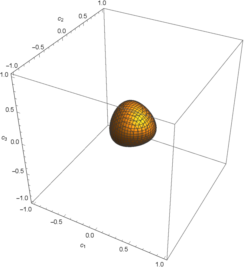
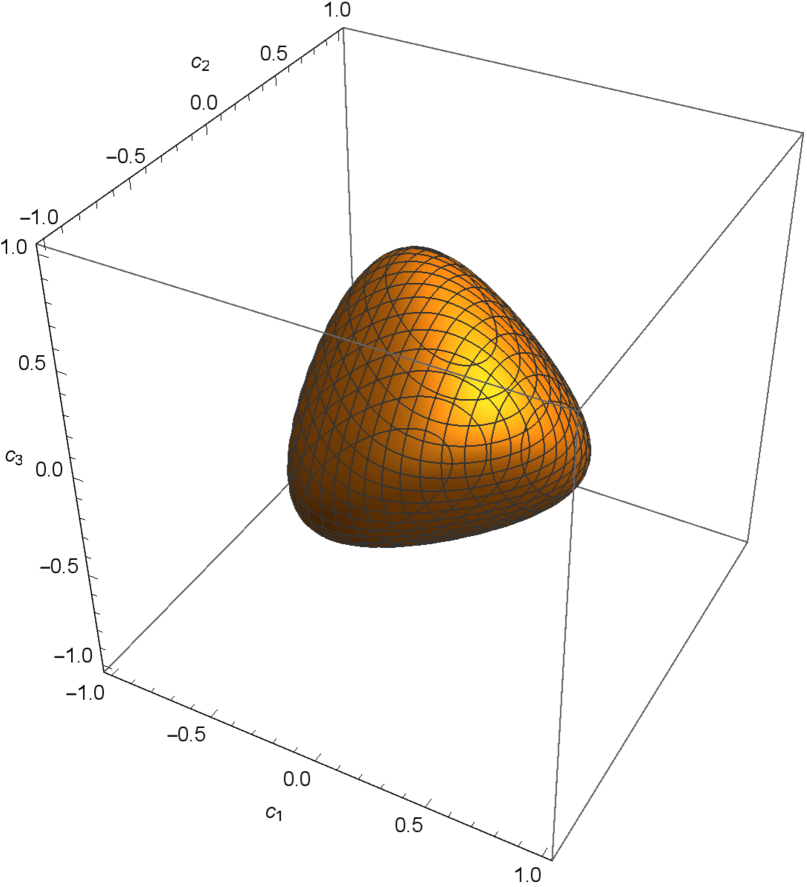
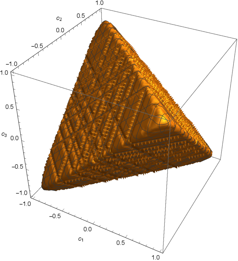
Figure 3: Surfaces of constant $C_{I}(\rho^{BD})_{a}$: (a) $C_{I}(\rho^{BD})_{a}=0.05$; (b) $C_{I}(\rho^{BD})_{a}=0.2$; (c) $C_{I}(\rho^{BD})_{a}=1$.

Now, we consider another special class of two qubit $X$ states. By taking $\mathbf{r}=(0,0,r)$ and $\mathbf{s}=(0,0,s)$, state (11) becomes the following one [61]

$$\rho^{X}_{z}=\frac{1}{4}\left(I\otimes I+r\sigma_{3}\otimes I+I\otimes s\sigma_{3}+\sum_{i=1}^{3}c_{i}\sigma_{i}\otimes\sigma_{i}\right),$$ (12)

which can be written as the following matrix in basis $a_{1}$

$$(\rho^{X}_{z})_{a_{1}}=\frac{1}{4}\left(\begin{array}[]{cccc}1+r+s+c_{3}&0&0&c_{1}-c_{2}\\ 0&1+r-s-c_{3}&c_{1}+c_{2}&0\\ 0&c_{1}+c_{2}&1-r+s-c_{3}&0\\ c_{1}-c_{2}&0&0&1-r-s+c_{3}\\ \end{array}\right).$$

Direct computation shows that

$$C_{I}(\rho^{X}_{z})_{a_{1}}$$ (13)

$$= 1-\frac{1}{16}\frac{1}{(c_{1}+c_{2})^{2}+(r-s)^{2}}\left[\left(\sqrt{1-c_{3}+\sqrt{(c_{1}+c_{2})^{2}+(r-s)^{2}}}(r-s+\sqrt{(c_{1}+c_{2})^{2}+(r-s)^{2}})\right.\right.$$

$$\left.+\sqrt{1-c_{3}-\sqrt{(c_{1}+c_{2})^{2}+(r-s)^{2}}}(-r+s+\sqrt{(c_{1}+c_{2})^{2}+(r-s)^{2}})\right)^{2}$$

$$+\left(\sqrt{1-c_{3}-\sqrt{(c_{1}+c_{2})^{2}+(r-s)^{2}}}(r-s+\sqrt{(c_{1}+c_{2})^{2}+(r-s)^{2}})\right.$$

$$\left.\left.+\sqrt{1-c_{3}+\sqrt{(c_{1}+c_{2})^{2}+(r-s)^{2}}}(-r+s+\sqrt{(c_{1}+c_{2})^{2}+(r-s)^{2}})\right)^{2}\right]$$

$$-\frac{1}{16}\frac{1}{(c_{1}-c_{2})^{2}+(r+s)^{2}}\left[\left(\sqrt{1+c_{3}+\sqrt{(c_{1}-c_{2})^{2}+(r+s)^{2}}}(-r-s+\sqrt{(c_{1}-c_{2})^{2}+(r+s)^{2}})\right.\right.$$

$$\left.+\sqrt{1+c_{3}+\sqrt{(c_{1}-c_{2})^{2}+(r+s)^{2}}}(r+s+\sqrt{(c_{1}-c_{2})^{2}+(r+s)^{2}})\right)^{2}$$

$$+\left(\sqrt{1+c_{3}-\sqrt{(c_{1}-c_{2})^{2}+(r+s)^{2}}}(r+s-\sqrt{(c_{1}-c_{2})^{2}+(r+s)^{2}})\right.$$

$$\left.\left.-\sqrt{1+c_{3}+\sqrt{(c_{1}-c_{2})^{2}+(r+s)^{2}}}(r+s+\sqrt{(c_{1}-c_{2})^{2}+(r+s)^{2}})\right)^{2}\right].$$

The surfaces of constant $C_{I}(\rho^{X}_{z})_{a_{1}}$ are shown in Figure 4. It can be seen that for $r=s$, the volume given by the surfaces expands for larger coherence, see Figures 4(a) and (c) or (b) and (d).

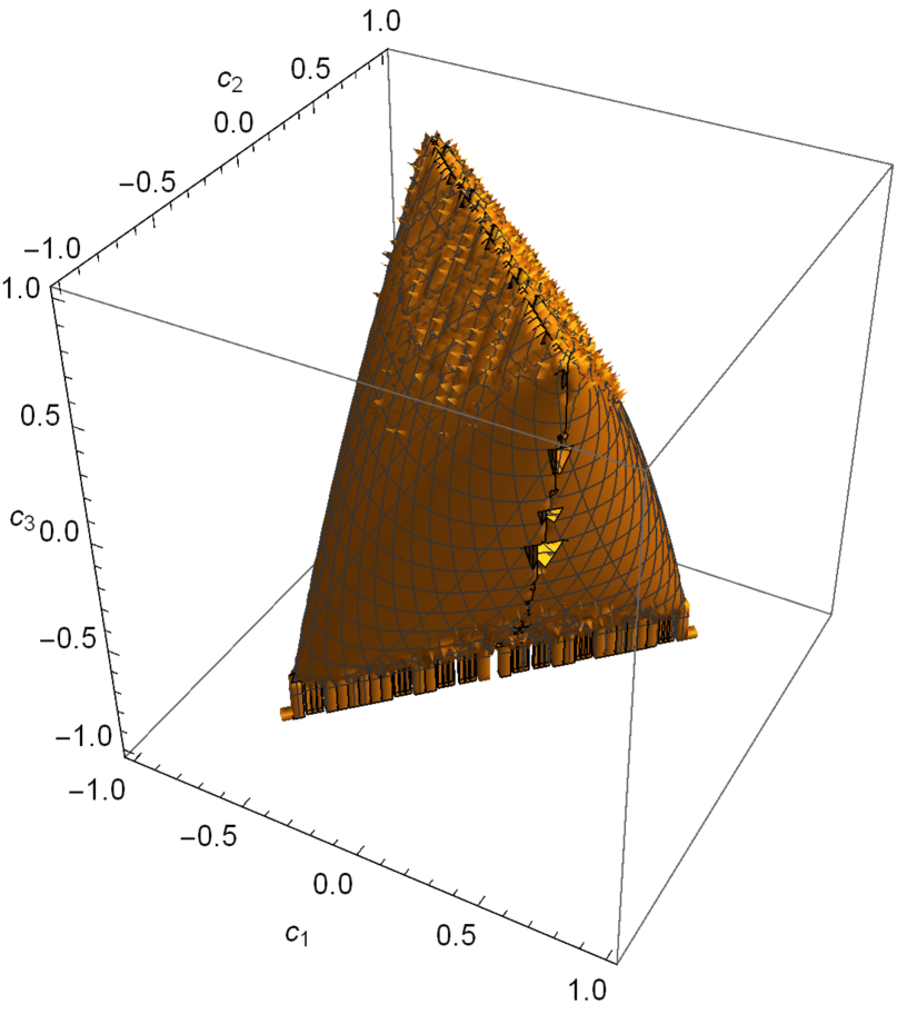
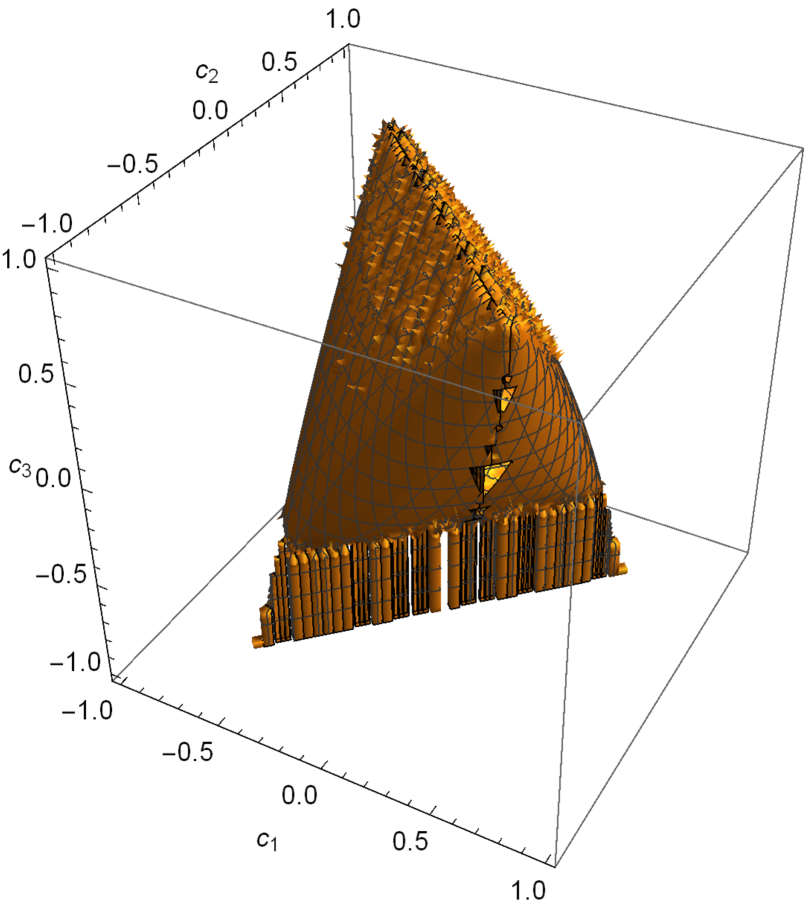
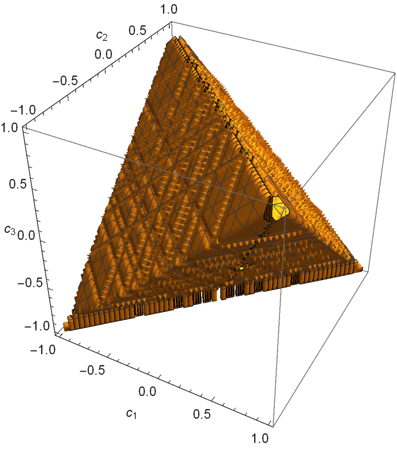
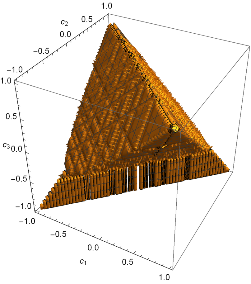
Figure 4: Surfaces of constant $C_{I}(\rho^{X}_{z})_{a_{1}}$ with fixed $r$ and $s$: (a) $r=s=0.1,C_{I}(\rho^{X}_{z})_{a_{1}}=0.1$; (b) $r=s=0.3,C_{I}(\rho^{X}_{z})_{a_{1}}=0.1$; (c) $r=s=0.1,C_{I}(\rho^{X}_{z})_{a_{1}}=0.5$; (d) $r=s=0.3,C_{I}(\rho^{X}_{z})_{a_{1}}=0.5$.

Similarly, the matrix form of (12) in basis $a_{2}$ and $a_{3}$ are

$$(\rho^{X}_{z})_{a_{2}}=\frac{1}{4}\left(\begin{array}[]{cccc}1+c_{1}&s&r&c_{3}-c_{2}\\ s&1-c_{1}&c_{2}+c_{3}&r\\ r&c_{2}+c_{3}&1-c_{1}&s\\ c_{3}-c_{2}&r&s&1+c_{1}\\ \end{array}\right)$$

and

$$(\rho^{X}_{z})_{a_{3}}=\frac{1}{4}\left(\begin{array}[]{cccc}1+c_{2}&s&r&c_{3}-c_{1}\\ s&1-c_{2}&c_{1}+c_{3}&r\\ r&c_{1}+c_{3}&1-c_{2}&s\\ c_{3}-c_{1}&r&s&1+c_{2}\\ \end{array}\right),$$

respectively, and $C_{I}(\rho^{X}_{z})_{a_{2}}$ and $C_{I}(\rho^{X}_{z})_{a_{3}}$ can be similarly calculated.

Moreover, denoting the sum of the skew information-based coherence of $\rho^{X}_{z}$ in bases $\{a_{i}\}_{i=1}^{3}$ by

$$C_{I}(\rho^{X}_{z})_{a}=C_{I}(\rho^{X}_{z})_{a_{1}}+C_{I}(\rho^{X}_{z})_{a_{2}}+C_{I}(\rho^{BD})_{a_{3}},$$ (14)

we obtain that

$$C_{I}(\rho^{X}_{z})_{a}$$ (15)

$$= \frac{1}{4}\left(6-\sqrt{1-\sqrt{\left(c_{1}+c_{2}\right){}^{2}+(r-s)^{2}}-c_{3}}\sqrt{1+\sqrt{\left(c_{1}+c_{2}\right){}^{2}+(r-s)^{2}}-c_{3}}\right.$$

$$\left.-\sqrt{1-\sqrt{\left(c_{1}-c_{2}\right){}^{2}+(r+s)^{2}}+c_{3}}\sqrt{1+\sqrt{\left(c_{1}+c_{2}\right){}^{2}+(r-s)^{2}}-c_{3}}\right.$$

$$\left.\sqrt{1-\sqrt{\left(c_{1}-c_{2}\right){}^{2}+(r+s)^{2}}+c_{3}}\sqrt{1+\sqrt{\left(c_{1}+c_{2}\right){}^{2}+(r-s)^{2}}-c_{3}}\right.$$

$$\left.-\sqrt{1-\sqrt{\left(c_{1}+c_{2}\right){}^{2}+(r-s)^{2}}-c_{3}}\sqrt{1-\sqrt{\left(c_{1}-c_{2}\right){}^{2}+(r+s)^{2}}+c_{3}}\right.$$

$$\left.-\sqrt{1-\sqrt{\left(c_{1}+c_{2}\right){}^{2}+(r-s)^{2}}-c_{3}}\sqrt{1+\sqrt{\left(c_{1}-c_{2}\right){}^{2}+(r+s)^{2}}+c_{3}}\right.$$

$$\left.-\sqrt{1-\sqrt{\left(c_{1}-c_{2}\right){}^{2}+(r+s)^{2}}+c_{3}}\sqrt{1+\sqrt{\left(c_{1}-c_{2}\right){}^{2}+(r+s)^{2}}+c_{3}}\right),$$

and the surfaces of constant $C_{I}(\rho^{X}_{z})_{a}$ are shown in Figure 5. It can be seen that similar properties hold compared with the surfaces of constant $C_{I}(\rho^{X}_{z})_{a_{1}}$ in Figure 4.

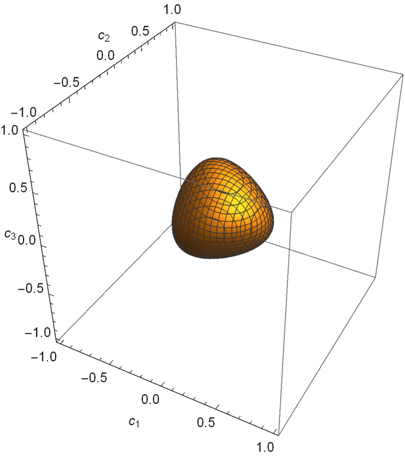
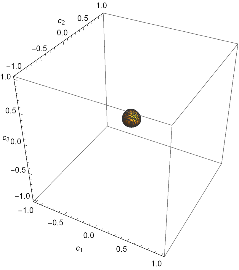
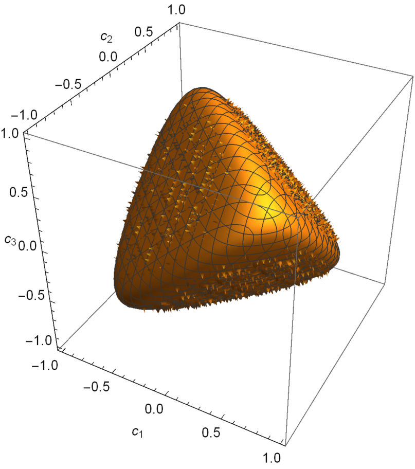
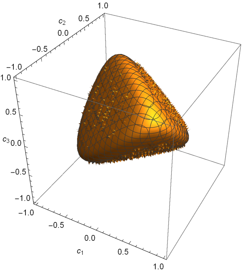
Figure 5: Surfaces of constant $C_{I}(\rho^{X}_{z})_{a}$ with fixed $r$ and $s$: (a) $r=s=0.1,C_{I}(\rho^{X}_{z})_{a}=0.1$; (b) $r=s=0.3,C_{I}(\rho^{X}_{z})_{a}=0.1$; (c) $r=s=0.1,C_{I}(\rho^{X}_{z})_{a}=0.5$; (d) $r=s=0.3,C_{I}(\rho^{X}_{z})_{a}=0.5$.

3. Skew information-based coherence under quantum channels

We now consider the evolution of the skew information-based quantum coherence under different quantum channels. Consider the following type of quantum channel $\Phi$:

$$\Phi(\rho)=\sum_{i,j}(E_{i}\otimes E_{j})\rho(E_{i}\otimes E_{j})^{\dagger},$$ (16)

where $\{E_{k}\}$ is the set of Kraus operators on a single qubit, satisfying $\sum_{k}E_{k}^{\dagger}E_{k}=I$. The Kraus operators for four kinds of quantum channels are listed in Table 1 [71].

Table 1: Kraus operators for the quantum channels: bit flip (BF), phase flip (PF), bit-phase flip (BPF), and generalized amplitude damping (GAD), where $p$ and $\gamma$ are decoherence probabilities, $0<p<1$, $0<\gamma<1$.

$$\begin{array}[]{ccccc}\hline\cr\hline\cr\text{Channel}&\text{Kraus operators}\\ \hline\cr\mathrm{BF}&E_{0}=\sqrt{1-p/2}I,\,\,\,\,\,\,E_{1}=\sqrt{p/2}\sigma_{1}\\ \mathrm{PF}&E_{0}=\sqrt{1-p/2}I,\,\,\,\,\,\,E_{1}=\sqrt{p/2}\sigma_{3}\\ \mathrm{BPF}&E_{0}=\sqrt{1-p/2}I,\,\,\,\,\,\,E_{1}=\sqrt{p/2}\sigma_{2}\\ \mathrm{GAD}&E_{0}=\sqrt{p}\left(\begin{array}[]{cc}1&0\\ 0&\sqrt{1-\gamma}\\ \end{array}\right),\,\,\,\,\,\,E_{2}=\sqrt{1-p}\left(\begin{array}[]{cc}\sqrt{1-\gamma}&0\\ 0&1\\ \end{array}\right)\\ &E_{1}=\sqrt{p}\left(\begin{array}[]{cc}0&\sqrt{\gamma}\\ 0&0\\ \end{array}\right),\,\,\,\,\,\,E_{3}=\sqrt{1-p}\left(\begin{array}[]{cc}0&0\\ \sqrt{\gamma}&0\\ \end{array}\right)\\ \hline\cr\hline\cr\end{array}$$

Noting that a Bell-diagonal state under BF, PF and BPF in Table 1 remains the same form, which is also the case under GAD for $p=1/2$ and any $\gamma$, we have

$$\Phi(\rho^{BD})=\frac{1}{4}(I\otimes I+\sum_{i=1}^{3}c_{i}^{\prime}\sigma_{i}\otimes\sigma_{i}),$$ (17)

where $\rho^{BD}$ is a two-qubit Bell-diagonal state, and the parameters $c_{i}^{\prime}$ $(i=1,2,3)$ are listed in Table 2 [71].

Table 2: Correlation coefficients with respect to the following channels: bit flip (BF), phase flip (PF), bit-phase flip (BPF), and generalized amplitude damping (GAD). For GAD, we have fixed $p=1/2$ and replaced $\gamma$ by $p$.

$$\begin{array}[]{ccccc}\hline\cr\hline\cr\text{Channel}&\text{$c_{1}^{\prime}$}&\text{$c_{2}^{\prime}$}&\text{$c_{3}^{\prime}$}\\ \hline\cr\mathrm{BF}&c_{1}&c_{2}(1-p)^{2}&c_{3}(1-p)^{2}\\ \mathrm{PF}&c_{1}(1-p)^{2}&c_{2}(1-p)^{2}&c_{3}\\ \mathrm{BPF}&c_{1}(1-p)^{2}&c_{2}&c_{3}(1-p)^{2}\\ \mathrm{GAD}&c_{1}(1-p)&c_{2}(1-p)&c_{3}(1-p)^{2}\\ \hline\cr\hline\cr\end{array}$$

By replacing $c_{i}$ by $c_{i}^{\prime}$ in Eq. (12), we plot the surfaces of constant $C_{I}(\Phi(\rho^{BD}))_{a_{1}}$ for the four types of channels by utilizing Table 2, see Figures 6, 7, 8 and 9. For simplicity, we use $C_{BF}$, $C_{PF}$, $C_{BPF}$ and $C_{GAD}$ to represent $C_{I}(\Phi(\rho^{BD}))_{a_{1}}$, where $\Phi$ is BF, PF, BPF and GAD, respectively. The surfaces show interesting shapes for parameter $p$ and the coherence $C$. When both $p$ and $C$ are small, the surface is very similar for four channels, see Figures 6-9(a). When $p$ is small and $C$ is large, the surface is two separate pieces of a tetrahedron with a gap in different directions for BF, PF and BPF channels, see Figures 6-8(b), and four pieces of a tetrahedron, see Figure 9(b). When $p$ is large and $C$ is small, the surface is two opposite surfaces for BF, PF and BPF channels, see Figures 6-8(c), and is four pieces of surfaces, of which two pairs are opposite for GAD channels, see Figure 9(c).

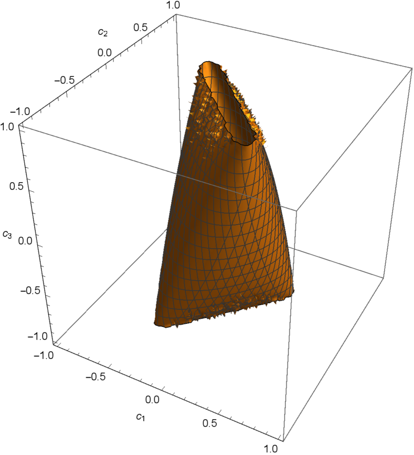
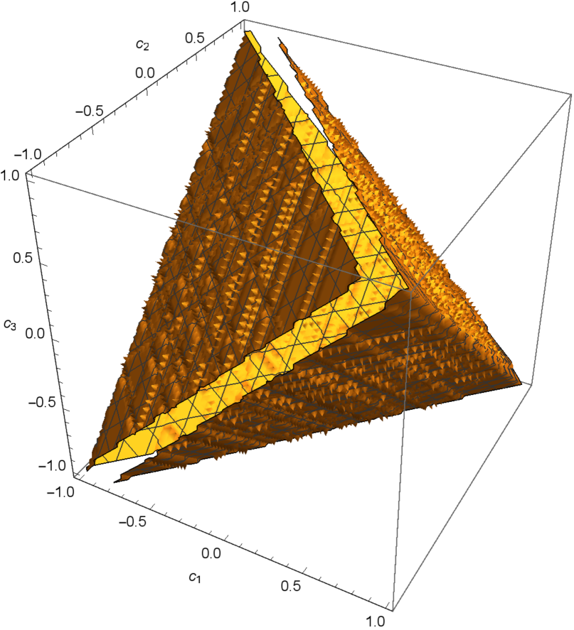
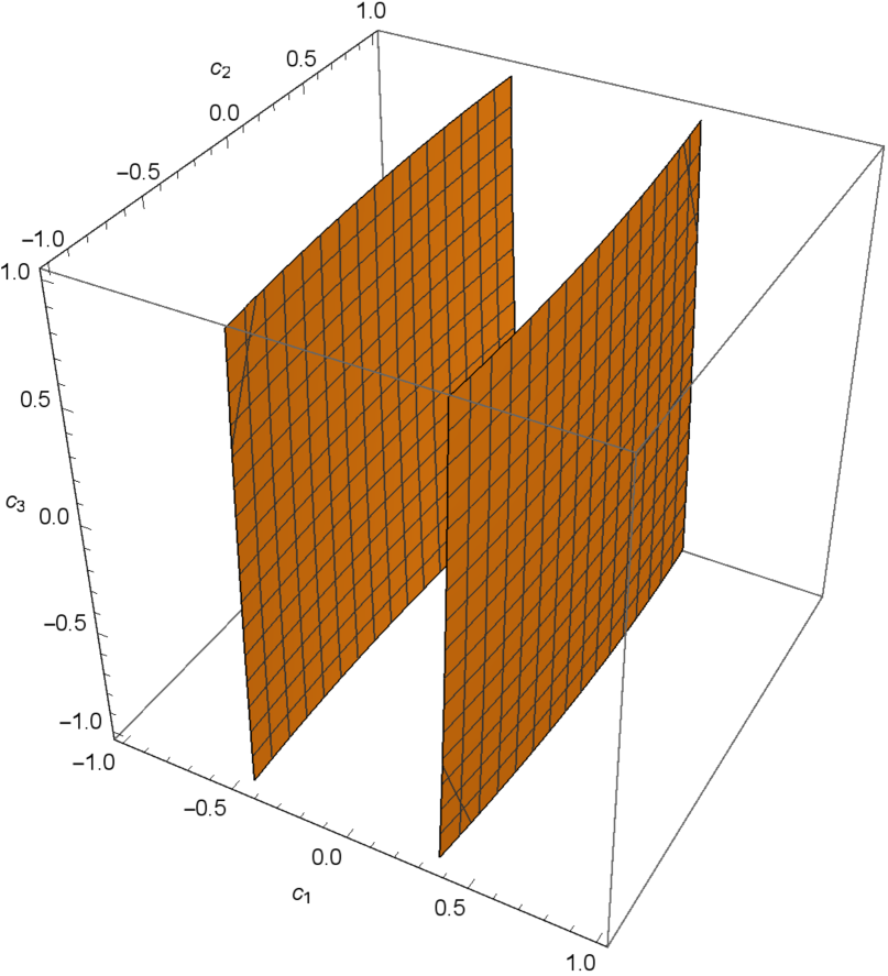
Figure 6: Surfaces of constant $C_{BF}$ for bit flip channels with fixed $p$: (a) $p=0.05,C_{BF}=0.05$; (b) $p=0.05,C_{BF}=0.4$; (c) $p=0.6,C_{BF}=0.05$.

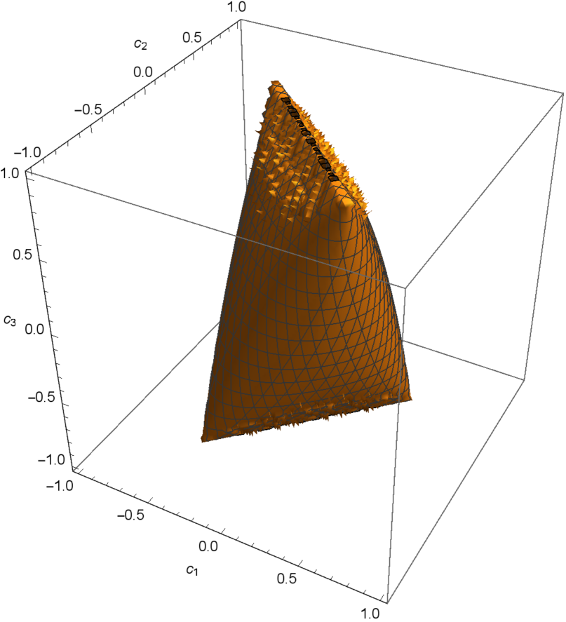
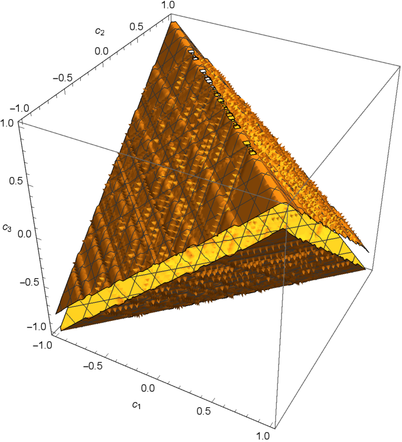
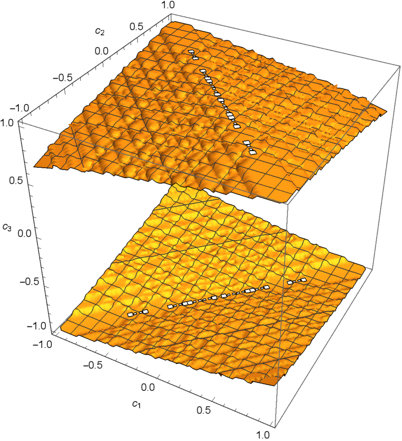
Figure 7: Surfaces of constant $C_{PF}$ for phase flip channels with fixed $p$: (a) $p=0.05,C_{PF}=0.05$; (b) $p=0.05,C_{PF}=0.4$; (c) $p=0.6,C_{PF}=0.05$.

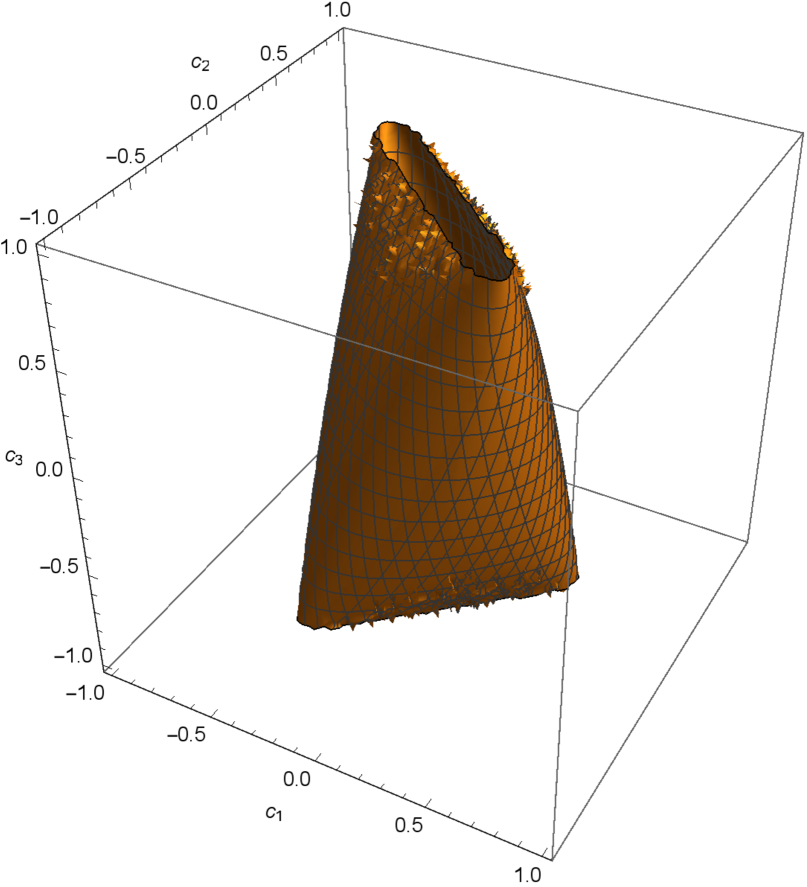
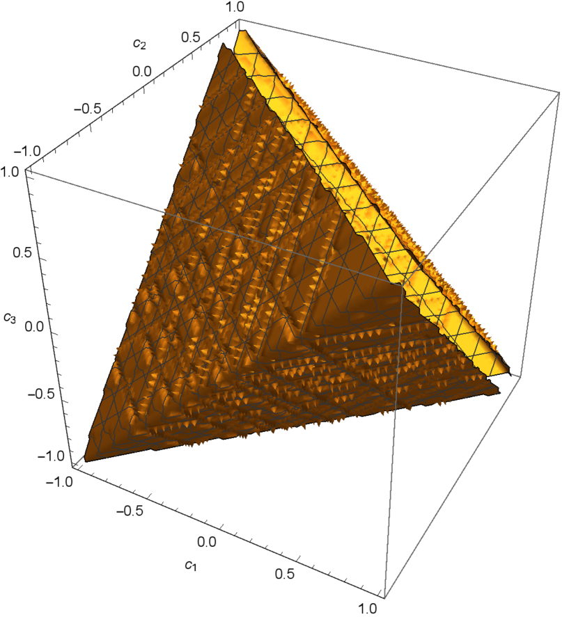
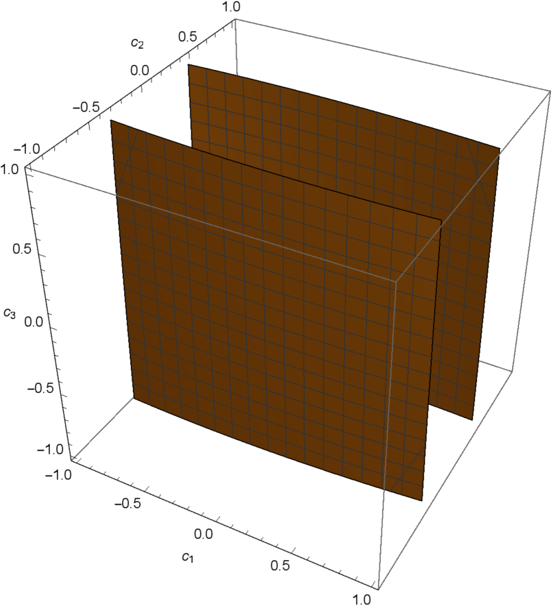
Figure 8: Surfaces of constant $C_{BPF}$ for bit-phase flip channels with fixed $p$: (a) $p=0.05,C_{BPF}=0.05$; (b) $p=0.05,C_{BPF}=0.4$; (c) $p=0.6,C_{BPF}=0.05$.

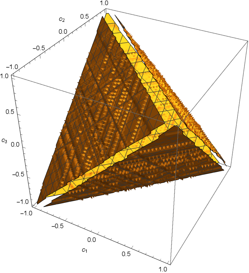
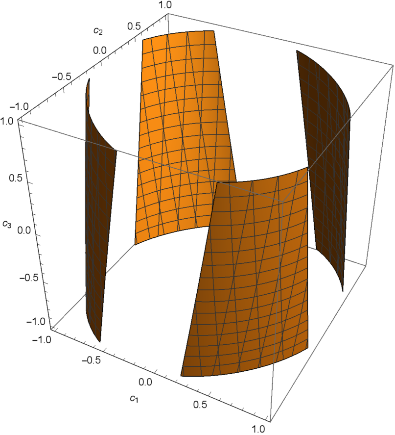
Figure 9: Surfaces of constant $C_{GAD}$ for generalized amplitude damping channels with fixed $p$: (a) $p=0.05,C_{GAD}=0.05$; (b) $p=0.05,C_{GAD}=0.4$; (c) $p=0.6,C_{GAD}=0.05$.

Setting $c_{1}=-0.2,c_{2}=0.6,c_{3}=0.6$ and $c_{1}=-0.6,c_{2}=0.2,c_{3}=0.2$, respectively, the dynamics of $C_{I}(\rho^{BD})$ under BF, PF, BPF and GAD channels are shown in Figure 10. The $C$-axis denotes $C_{BF},C_{PF},C_{BPF}$ and $C_{GAD}$. Similar to the case of relative entropy of coherence in [62], we find that all the curves are decreasing functions of $p$, and $C_{PF}$ and $C_{GAD}$ approaches to zero as $p$ approaches $1$. Moreover, $C_{BF}$ decreases dramatically as $p$ increases, see Figure 10(a), while it decreases very slowly in case of Figure 10(b).

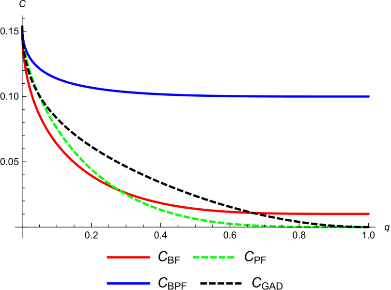
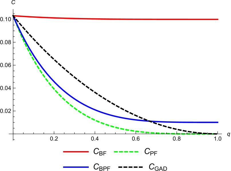
Figure 10: $C_{BF},C_{PF},C_{BPF}$ and $C_{GAD}$ as a function of $p$: (a) $c_{1}=-0.2,c_{2}=0.6,c_{3}=0.6$; (b) $c_{1}=-0.6,c_{2}=0.2,c_{3}=0.2$.

4. Conclusions and discussions

We have studied the geometry of skew information-based coherence of quantum states in mutually unbiased bases by calculating the skew information-based coherence for two qubit states. We calculated the analytical expression for Bell-diagonal states and a special class of $X$ states in a set of autotensor of mutually unbiased bases. As direct consequences, explicit formulas for coherences of Werner states and isotropic states have also been given, which shows that the former is an decreasing function of the state parameter, while the latter is not. Based on these, the geometry of skew information-based coherence for these two qubit states in both computational basis and in MUBs have been depicted.

Moreover, we have displayed the level surfaces of skew information-based coherence for Bell-diagonal states under four typical local nondissipative quantum channels. It has been shown that similar trend occurs when the relative entropy of coherence is used, but the shape of the graphics turned out to be very different. Furthermore, by choosing two different sets of fixed values for $c_{1}$, $c_{2}$ and $c_{3}$, we have depicted the skew information-based coherence under the four channels as a function of the parameter $p$. It shows the similar features as the relative entropy of coherence.

References

[1] T. Baumgratz, M. Cramer, and M. B. Plenio, Phys. Rev. Lett. 113 (2014)
140401.
[2] X. Yuan, H. Zhou, Z. Cao, and X. Ma,
Phys. Rev. A 92 (2015) 022124.
[3] C. Napoli, T. R. Bromley, M. Cianciaruso, et al., Phys. Rev. Lett.
116 (2016) 150502.
[4] K. Bu, U. Singh, S.-M. Fei, et al., Phys. Rev. Lett. 119 (2017) 150405.
[5] C. Xiong and J. Wu, J. Phys. A: Math. Theor. 51 (2018)
414005.
[6] X.-D. Yu, D.-J. Zhang, G. Xu, and D. Tong, Phys. Rev. A 94 (2016)
060302(R).
[7] B. Chen and S.-M. Fei, Quantum Inf. Process. 17 (2018)
107.
[8] C.-S. Yu, Phys. Rev. A 95 (2017) 042337.
[9] S. Luo and Y. Sun, Phys. Rev. A 96 (2017)
022130.
[10] S. Luo and Y. Sun, Phys. Rev. A 96 (2017) 022136.
[11] S. Luo and Y. Sun, Phys. Rev. A 98 (2018) 012113.
[12] K. Bu, N. Anand, and U. Singh, Phys. Rev. A 97 (2018) 032342.
[13] C. Xiong, A. Kumar, and J. Wu, Phys. Rev. A 98 (2018) 032324.
[14] C. Xiong, A. Kumar, M. Huang, et al., Phys. Rev. A 99 (2019) 032305.