Hierarchical Aggregation for 3D Instance Segmentation

Abstract

Instance segmentation on point clouds is a fundamental task in 3D scene perception. In this work, we propose a concise clustering-based framework named HAIS, which makes full use of spatial relation of points and point sets. Considering clustering-based methods may result in over-segmentation or under-segmentation, we introduce the hierarchical aggregation to progressively generate instance proposals, i.e., point aggregation for preliminarily clustering points to sets and set aggregation for generating complete instances from sets. Once the complete 3D instances are obtained, a sub-network of intra-instance prediction is adopted for noisy points filtering and mask quality scoring. HAIS is fast (only $410ms$ per frame) and does not require non-maximum suppression. It ranks 1st on the ScanNet v2 benchmark , achieving the highest $69.9\%$ $AP_{50}$ and surpassing previous state-of-the-art (SOTA) methods by a large margin. Besides, the SOTA results on the S3DIS dataset validate the good generalization ability. Code will be available at https://github.com/hustvl/HAIS.

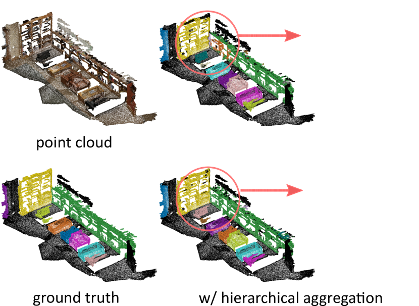
Figure 1: An input point cloud, ground truth instance masks and 3D instance prediction results without & with hierarchical aggregation. As shown in the key region circled with red, for objects with large sizes and fragmentary point clouds, the predictions are easy to be over-segmented. The proposed hierarchical aggregation combines incomplete instances with fragments to form complete instance predictions.

1 Introduction

With the rapid development and popularization of commodity 3D sensors (Kinect, RealSense, Velodyne laser scanner, etc.), 3D scene understanding has become a hot research topic in the field of computer vision. Instance segmentation on point cloud, as the basic perception task of 3D scene understanding, is the technical foundation of a wide range of real-life applications, e.g., robotics, augmented/virtual reality, and autonomous driving.

Instance segmentation on 2D images has been exhaustively studied in the past few years [7, 24, 16, 27, 18, 4, 5, 11]. Top-down methods dominate 2D instance segmentation. They first generate instance-level proposals and then predict the mask for each proposal. Though existing 2D instance segmentation methods can be directly extended to 3D scenes, most existing 3D methods adopt a totally different bottom-up pipeline [42, 41, 22, 15, 20], which generates instances through clustering.

However, directly clustering a point cloud into multiple instances is very difficult for the following reasons: $(1)$ A point cloud usually contains a large number of points; $(2)$ The number of instances in a point cloud has large variations for different 3D scenes; $(3)$ The sizes of instances vary significantly; $(4)$ Each point has a very weak feature, i.e., 3D coordinate and color. The semantic gap between point and instance identity is huge. Thus, over-segmentation or under-segmentation are common problems and are prone to exist.

We propose a hierarchical aggregation scheme in bottom-up 3D instance segmentation networks to cope with these problems. We first aggregate points to sets with low bandwidth to avoid over-segmentation and then set aggregation with dynamic bandwidth is adopted to form complete instances. Set aggregation may absorb noisy point sets into predictions, making the aggregated instances over-complete. Thus, we design a sub-network for outlier filtering and mask quality scoring. Based on the hierarchical aggregation and the sub-network for intra-instance prediction, we propose a novel bottom-up framework, named HAIS. HAIS achieves the state-of-the-art (SOTA) performance on both the ScanNet v2 benchmark [6] and the S3DIS [1] dataset. Beyond this, HAIS is efficient, only requiring a concise single-forward inference without any post-processing steps. Compared with all the existing methods, HAIS takes the lowest inference latency.

Our contributions can be summarized as follows.

• We propose a novel bottom-up framework with the hierarchical aggregation for instance segmentation on 3D point cloud. The hierarchical aggregation strategy makes up the defects of bottom-up clustering. Besides, an intra-instance prediction network is designed for generating more fine-grained instance predictions.

• Our method ranks 1st on the leaderboard of ScanNet v2 [6]. HAIS also achieves the state-of-the-art result on S3DIS [1]. We significantly promote the performances on various challenging datasets and demonstrate the generalization of the proposed methods.

• Our method achieves the highest efficiency among all existing methods. HAIS keeps a concise single-forward inference pipeline without any post-processing steps. The average per-frame inference time on ScanNet v2 is only $410$ ms, much faster than other methods.

2 Related Works

Deep Learning on Point Clouds

Extracting features from point clouds is the foundation of 3D scene understanding. Deep learning equipped methods mainly include point-based ones and voxel-based ones. Point-based methods, e.g., PointNet [35] and PointNet++ [36], directly operate on unstructured sets of points. Voxel-based methods [14, 38, 40, 30] transform the unordered and unstructured point sets to ordered and structured volumetric grids, and then perform 3D sparse convolutions on the grids. We adopt voxel-based methods for more efficient feature extraction.

Proposal-based Instance Segmentation

Proposal-based approaches directly generate object proposals and predict masks inside each proposal. In the 2D domain, proposal-based methods employ 2D object detectors [13, 37, 8, 25] to generate region proposals and then predict masks inside each proposal. Mask R-CNN [16] extends Faster R-CNN [37] by adding a mask prediction. EmbedMask [45] introduces proposal embedding and pixel embedding so that pixels are assigned to instance proposals according to their embedding similarity. In the 3D domain, GSPN [44] proposes a generative shape proposal network for 3D object proposals following an analysis-by-synthesis strategy. 3D-SIS [17] takes both 3D geometry and 2D color images as input and combines 2D and 3D features through the back projection for a better prediction. 3D-BoNet [43] regresses a fixed set of bounding boxes and designs a novel association layer to match predicted boxes and ground truth boxes. 3D-MPA [9] predicts centers of instances and employs a graph convolutional network to refine proposal features. GICN [28] approximates the distributions of instance centers as Gaussian center heatmaps and uses a center selection mechanism for choosing candidates.

Figure 2: The framework of HAIS. For the input point cloud, our method first employs 3D UNet-like structure with submanifold sparse convolution [39, 14] for point-wise feature learning. Then, we use the spatial constraint of points to perform point aggregation with fixed bandwidth. Based on point aggregation results, set aggregation with dynamic bandwidth is performed to form instance proposals. The intra-instance prediction is designed for outlier filtering and mask quality scoring.

Clustering-based Instance Segmentation

Clustering-based approaches first predict point-wise labels and then use clustering methods to generate instance predictions. In the 2D domain, metric learning is widely used to group pixels. Fathi et al. [12] compute likelihoods of pixels and group similar pixels together within an embedding space. Bai and Urtasun [2] adopt energy maps to distinguish among individual instances. Kong and Fowlkes [21] assign all pixels to a spherical embedding for clustering. Neven et al. [33] introduce a learnable clustering bandwidth instead of learning the embedding using hand-crafted cost functions. Bert et al. [3] propose a discriminative loss function which encourages the network to map each pixel to a point in feature space so that pixels belonging to the same instance lie close together while different instances are separated by a wide margin. In the 3D domain, SGPN [41] proposes to learn a similarity matrix for all point pairs and merges similar points to generate instances. JSIS3D [34] adopts multi-value conditional random fields to form instance predictions. MTML [22] introduces a multi-task learning strategy for grouping points. OccuSeg [15] adopts learnt occupancy signals to guide clustering. PointGroup [20] proposes to cluster points based on dual coordinate sets and designs ScoreNet to predict scores for instances.

Our HAIS follows the clustering-based paradigm but differs from existing clustering-based methods in two terms. First, most clustering-based methods require complicated and time-consuming clustering procedures, but our HAIS adopts a much more concise pipeline and keeps high efficiency. Second, previous methods usually group points according to point-level embeddings, without the instance-level correction. Our HAIS introduces the set aggregation and intra-instance prediction to refine the instance at the object level.

3 Method

The overall architecture of HAIS is depicted in Fig. 2, which consists of four main parts. The point-wise prediction network (Sec. 3.1) extracts features from point clouds and predicts point-wise semantic labels and center shift vectors. The point aggregation module (Sec. 3.2) forms preliminary instance predictions based on point-wise prediction results. The set aggregation module (Sec. 3.3) expands incomplete instances to cover missing parts, while the intra-instance prediction network (Sec. 3.4) smooths instances to filter out outliers.

3.1 Point-wise Prediction Network

The point-wise prediction network takes the point cloud $P\in\mathbb{R}^{N\times K}$ as input, where $N$ is the number of points and $K$ is the number of channels. $K$ is normally set as 6 for colors $r$, $g$, $b$ and locations $x$, $y$, $z$. The submanifold sparse convolution [14] is widely used in 3D perception methods [20, 22, 26, 9] to extract features from point clouds. Following the common practice, we first convert the point cloud data into regular volumetric grids. Then a UNet-like structure [39] composed of stacked 3D sparse convolution layers [14] is used to extract voxel features $F_{\text{voxel}}$. Third, we map the voxel features $F_{\text{voxel}}$ back to point features $F_{\text{point}}$. Based on point features $F_{\text{point}}$, two branches are built, one for predicting point labels and the other for predicting the per-point center shift vectors.

Semantic Label Prediction Branch

We apply a 2-layer Multi-Layer Perception (MLP) with a softmax layer upon $F_{\text{point}}$ to produce semantic scores for every class. The class with the highest score will be regraded as the predicted point label. The cross-entropy loss of semantic scores $\mathcal{L}_{\text{seg}}$ is used to train this branch.

Center Shift Vector Prediction Branch

Paralleled with the semantic label prediction branch, we apply a 2-layer MLP upon $F_{\text{point}}$ to predict the point-wise center shift vector $\triangle x_{i}$ ($\triangle x_{i}\in\mathbb{R}^{3}$), which represents the offset from each point to its instance center, similar to [9, 20]. The instance center is defined as the coordinate mean of all points in this instance. During training, $\mathcal{L}_{\text{shift}}$ is used to optimize the center shift vector prediction, which is formulated as

$$\mathcal{L}_{\text{shift}}=\frac{1}{\sum\limits_{p_{i}\in P}\mathbbm{1}(p_{i}\in P_{\text{fg}})}\cdot\sum\limits_{p_{i}\in P}\mathcal{L}(p_{i})\text{,}$$ (1)

$$\mathcal{L}(p_{i})=w(p_{i})\cdot{\parallel\triangle x^{\text{gt}}_{i}-\triangle x^{\text{pred}}_{i}\parallel}_{1}\cdot\mathbbm{1}(p_{i}\in P_{\text{fg}})\text{,}$$

$$w(p_{i})=\min({\parallel\triangle x^{\text{gt}}_{i}\parallel}_{2},1)\text{.}$$

$\mathbbm{1}(\cdot)$ is the indicator function. $P$ and $P_{\text{fg}}$ denote the whole point set and the foreground point set respectively. Background points are ignored in $\mathcal{L}_{\text{shift}}$. $w(p_{i})$ serves as a point-wise weighted term. Points closer to the instance center less rely on the center shift vectors and should contribute less to the loss.

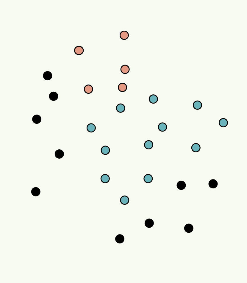
(a) original coordinates

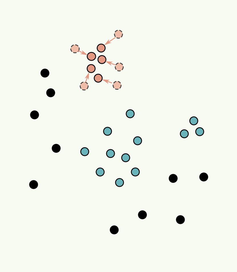
(b) shifted coordinates

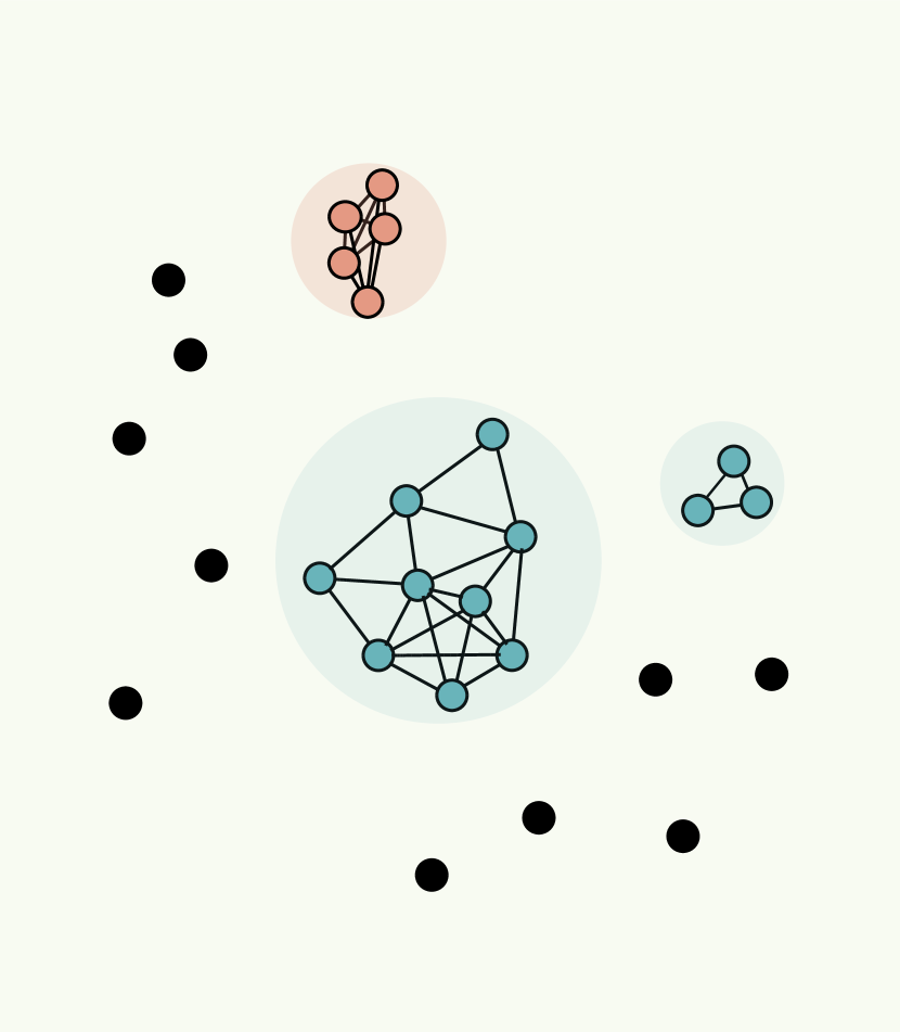
(c) point aggregation

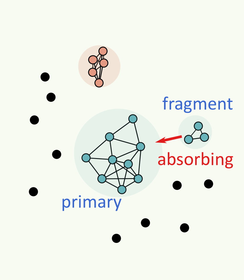
(d) set aggregation

Figure 3: Illustrations of hierarchical aggregation. Points with different colors belong to different categories. Black points belong to background. (a): Points distributed in real 3D space. (b): After applying the center shift vector to each point, points belong to the same instance are closer in 3D space. (c): Point aggregation. Aggregating points into sets based on fixed spatial clustering bandwidth. (d): Set aggregation. Primary instances absorb surrounding fragments with dynamic clustering bandwidth to form complete instances.

3.2 Point Aggregation

In the 3D space, points of the same instance are inherently adjacent to each other. It’s intuitive to utilize this spatial constraint for clustering. Thus, based on the semantic label and the center shift vector, we use a basic and compact clustering method to get preliminary instances. First, as shown in Fig. 3(b), according to the point-wise center shift vector $\triangle x_{i}$, we shift every point $x^{\text{origin}}_{i}$ toward its instance center, making the points of the same instance spatially closer to each other. The shifted coordinate is computed as,

$${x^{\text{shift}}_{i}}={x^{\text{origin}}_{i}}+\triangle x_{i}\text{.}$$ (2)

Second, we ignore background points and regard each foreground point as a node. For every pair of nodes, if they have the same semantic label and their spatial distance is smaller than a fixed spatial clustering bandwidth $r_{\text{point}}$, an edge between these two nodes is created. After traversing all the pairs of node and establishing edges, the whole point cloud is separated into multiple independent sets, as shown in Fig. 3(c). Each set can be viewed as a preliminary instance prediction.

3.3 Set Aggregation

Fig. 4 shows the distribution of instance size (the number of points in an instance) of the ground truth and the point aggregation results. Compared with the sizes of ground truth instances, point aggregation generates a much larger number of instance predictions with small sizes. It is because center shift vectors are not totally accurate. Point aggregation cannot guarantee that all the points in an instance are grouped together. As illustrated in Fig. 3(d), most points with accurate center shift vectors can be clustered together to form incomplete instance predictions. We call these instances “primary instances”. But a minority of points with poor center shift vector predictions split from the majority and form fragmentary instances with small sizes, which we call “fragments”. Fragments are too small in size to be regarded as complete instances, but are possible to be the missing part of primary instances. Considering the large number of fragments, it’s not appropriate to directly filter out fragments with a hard threshold. Intuitively, we can aggregate primary instances and fragments at set level to generate complete instance predictions.

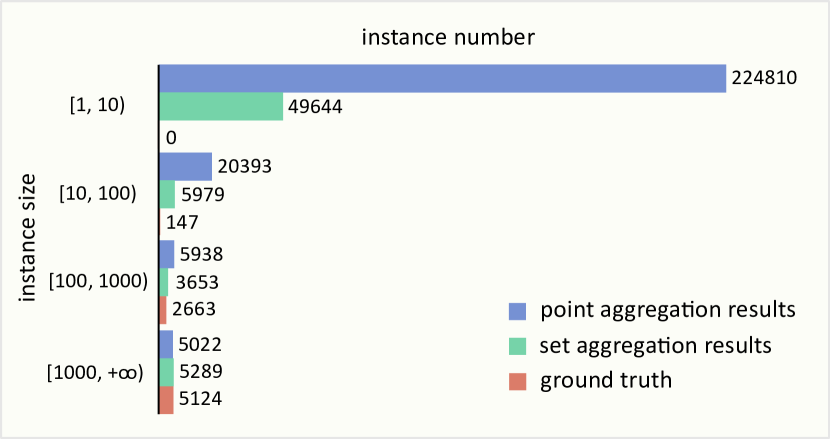
Figure 4: Distribution of instance size. The instance size is defined as the number of points inside an instance. Blue, green and red correspond to point aggregation results, set aggregation results and ground truth, respectively. The statistics are based on the ScanNet v2 [6] validation set.

Based on the above clues, we propose the set aggregation to smooth the instance predictions generated by point aggregation, which is shown in Fig. 3(d). The detailed procedure is provided in Alg. 1. Briefly, if the following two conditions are satisfied, we consider the fragment $m$ to be a part of the primary instance $n$. First, among all the primary instances that have the same semantic label with the fragment $m$, the primary instance $n$ is the one whose geometric center is closest to the fragment $m$. Secondly, for the fragment $m$ and the primary instance $n$, the distance between their geometric center should be smaller than $r_{\text{set}}$, which is the dynamic clustering bandwidth defined as,

$$r_{\text{set}} =\max(r_{\text{size}},r_{\text{cls}}),$$ (3)

$$r_{\text{size}} =\alpha\sqrt{S^{n}_{\text{prim}}}.$$

The clustering bandwidth of set aggregation is determined by $r_{\text{size}}$ and $r_{\text{cls}}$. $r_{\text{size}}$ denotes the size-specific bandwidth. It is reasonable that the larger primary instances should absorb fragments in a wider range, and we consider $r_{\text{size}}$ relative to the square root of the primary instance $n$’s size $S^{n}_{\text{prim}}$. $r_{\text{cls}}$ denotes the class-specific bandwidth, which is the statistical average instance radii of the specific class. The distribution of instance size after the set aggregation is shown in Fig. 4. A large amount of fragments are combined together with primary instances to form instances with higher quality.

Data:

Fragments: $\{I^{1}_{\text{frag}},I^{2}_{\text{frag}},...,I^{N_{\text{frag}}}_{\text{frag}}\}$

Primary instances: $\{I^{1}_{\text{prim}},I^{2}_{\text{prim}},...,I^{N_{\text{prim}}}_{\text{prim}}\}$

Centers of fragments: $\{c^{1}_{\text{frag}},c^{2}_{\text{frag}},...,c^{N_{\text{frag}}}_{\text{frag}}\}$

Centers of primary instances: $\{c^{1}_{\text{prim}},c^{2}_{\text{prim}},...,c^{N_{\text{prim}}}_{\text{prim}}\}$

Class labels of fragments : $\{L^{1}_{\text{frag}},L^{2}_{\text{frag}},...,L^{N_{\text{frag}}}_{\text{frag}}\}$

Class labels of primary instances: $\{L^{1}_{\text{prim}},L^{2}_{\text{prim}},...,L^{N_{\text{prim}}}_{\text{prim}}\}$

Dynamic set aggregation bandwidths: $\{r^{1}_{\text{set}},r^{2}_{\text{set}},...,r^{N_{\text{prim}}}_{\text{set}}\}$

Result:

A set of refined instances: $\{I^{1}_{\text{prim}},I^{2}_{\text{prim}},...,I^{N_{\text{prim}}}_{\text{prim}}\}$

1

2for $m=1\to N_{\rm frag}$ do

3       ${\rm index}=-1$

4       $d_{\text{min}}=+\infty$

5       for $n=1\to N_{\rm prim}$ do

6             if  $L^{m}_{\rm frag}==L^{n}_{\rm prim}$ and

7             $\|c^{m}_{\rm frag}-c^{n}_{\rm prim}\|<d_{\rm min}$  then

8                   ${\rm index}=n$

9                   $d_{\text{min}}=\|c^{m}_{\text{frag}}-c^{n}_{\text{prim}}\|$

10                  

11             end if

12            

13       end for

14      if  $d_{\rm min}<r^{\rm index}_{\rm set}$ then

15             $I^{\text{index}}_{\text{prim}}=I^{\text{index}}_{\text{prim}}\cup I^{m}_{\text{frag}}$

16       end if

17      

18 end for

return $\{I^{1}_{\rm prim},I^{2}_{\rm prim},...,I^{N_{\rm prim}}_{\rm prim}\}$

Algorithm 1 Set aggregation. $N_{\text{frag}}$ is the number of fragments. $N_{\text{prim}}$ is the number of primary instances.

Figure 5: The details of the intra-instance prediction network.

Method	$AP_{50}$	bathtub	bed	bookshe.	cabinet	chair	counter	curtain	desk	door	otherfu.	picture	refrige.	s. curtain	sink	sofa	table	toilet	window
DPC [10]	35.5	50.0	51.7	46.7	22.8	42.2	13.3	40.5	11.1	20.5	24.1	7.5	23.3	30.6	44.5	43.9	45.7	97.4	23.0
3D-SIS [17]	38.2	100.0	43.2	24.5	19.0	57.7	1.3	26.3	3.3	32.0	24.0	7.5	42.2	85.7	11.7	69.9	27.1	88.3	23.5
MASC [26]	44.7	52.8	55.5	38.1	38.2	63.3	0.2	50.9	26.0	36.1	43.2	32.7	45.1	57.1	36.7	63.9	38.6	98.0	27.6
PanopticFusion [32]	47.8	66.7	71.2	59.5	25.9	55.0	0.0	61.3	17.5	25.0	43.4	43.7	41.1	85.7	48.5	59.1	26.7	94.4	35.0
3D-BoNet [43]	48.8	100.0	67.2	59.0	30.1	48.4	9.8	62.0	30.6	34.1	25.9	12.5	43.4	79.6	40.2	49.9	51.3	90.9	43.9
MTML [22]	54.9	100.0	80.7	58.8	32.7	64.7	0.4	81.5	18.0	41.8	36.4	18.2	44.5	100.0	44.2	68.8	57.1	100.0	39.6
3D-MPA [9]	61.1	100.0	83.3	76.5	52.6	75.6	13.6	58.8	47.0	43.8	43.2	35.8	65.0	85.7	42.9	76.5	55.7	100.0	43.0
PointGroup [20]	63.6	100.0	76.5	62.4	50.5	79.7	11.6	69.6	38.4	44.1	55.9	47.6	59.6	100.0	66.6	75.6	55.6	99.7	51.3
GICN [28]	63.8	100.0	89.5	80.0	48.0	67.6	14.4	73.7	35.4	44.7	40.0	36.5	70.0	100.0	56.9	83.6	59.9	100.0	47.3
HAIS	69.9	100.0	84.9	82.0	67.5	80.8	27.9	75.7	46.5	51.7	59.6	55.9	60.0	100.0	65.4	76.7	67.6	99.4	56.0

Table 1: Quantitative comparison on the testing set of ScanNet v2 [6] benchmark. Our HAIS achieves the SOTA performance, outperforming all other methods by a large margin.

Method	mCov	mWCov	mPrec	mRec
SGPN† [41]	32.7	35.5	36.0	28.7
ASIS† [42]	44.6	47.8	55.3	42.4
PointGroup† [20]	-	-	61.9	62.1
HAIS†	64.3	66.0	71.1	65.0
SGPN‡ [41]	37.9	40.8	38.2	31.2
PartNet‡ [31]	-	-	56.4	43.4
ASIS‡ [42]	51.2	55.1	63.6	47.5
3D-BoNet‡ [43]	-	-	65.6	47.6
OccuSeg‡ [15]	-	-	72.8	60.3
GICN‡ [28]	-	-	68.5	50.8
PointGroup‡ [20]	-	-	69.6	69.2
HAIS‡	67.0	70.4	73.2	69.4

Table 2: Quantitative comparison on S3DIS [1]. Methods marked with $\dagger$ are evaluated on Area 5 and those marked with $\ddagger$ are on the 6-fold cross validation. Our method significantly outperforms previous methods in terms of mCov (coverage), mWCov (weighted coverage), mean precision (mPrec) and mean recall (mRec).

3.4 Intra-instance Prediction Network

The hierarchical aggregation may mistakenly absorb fragments belonging to other instances, generating inaccurate instance predictions. Thus, we propose the intra-instance prediction network for further refining the instances, as shown in Fig. 5. First, we crop instance point cloud patches as input and use the 3D submanifold sparse convolution network to extract features inside instances. After intra-instance feature extraction, the mask branch predicts binary masks to distinguish the instance foreground and background. For every predicted instance, we choose the best matched GT (ground truth) as the mask supervision. The overlapped parts between the predicted instance and the GT are assigned with positive labels, and others are assigned with negative labels. Low quality instances (low IoU with GT) contain little instance-level information and are valueless to optimizing the mask branch. Thus, only the instances with IoU higher than $0.5$ are used as training samples, while others are ignored. For mask prediction, the loss is formulated as,

$$\mathcal{L}_{\text{mask}}= -\frac{1}{\sum\limits^{N_{\text{ins}}}\limits_{i=1}\mathbbm{1}(iou_{i}>0.5)\cdot N_{i}}\cdot\sum\limits^{N_{\text{ins}}}\limits_{i=1}\Big{\{}\mathbbm{1}(iou_{i}>0.5)$$ (4)

$$\cdot\sum\limits^{N_{i}}\limits_{j=1}\big{[}y_{j}\cdot\log(\hat{y}_{j})+(1-y_{j})\cdot\log(1-\hat{y}_{j})\big{]}\Big{\}},$$

where $N_{\text{ins}}$ denotes the number of instances and $N_{i}$ denotes the point number of instance $i$.

Besides mask prediction, the instance certainty score is needed for ranking among instances. We utilize masks for better scoring instances, as illustrated in Fig. 5. Firstly, masks are used to filter out features of background point, which would be noise for scoring. The remained foreground features are sent into a MLP with a sigmoid layer to predict the instance certainty scores. Secondly, inspired by [18, 19, 23], we regard the IoUs between predicted masks and GT masks as the mask quality and use them to supervise instance certainty. For the score prediction, the loss is formulated as,

$$\mathcal{L}_{\text{score}}= -\frac{1}{N_{\text{ins}}}\cdot\sum\limits^{N_{\text{ins}}}\limits_{i=1}\big{[}iou_{i}\cdot\log(\hat{s}_{i})$$ (5)

$$+(1-iou_{i})\cdot\log(1-\hat{s}_{i})\big{]}.$$

Ablation studies in Sec. 4.4 further demonstrate that using masks to assist score prediction boosts performance.

3.5 Multi-task Training

The whole network is trained from scratch in an end-to-end manner and optimized by a joint loss consisting of several loss terms,

$$\mathcal{L}=\mathcal{L}_{\text{seg}}+\mathcal{L}_{\text{shift}}+\mathcal{L}_{\text{mask}}+\mathcal{L}_{\text{score}},$$ (6)

where $\mathcal{L}_{\text{seg}}$ is the cross-entropy loss of semantic scores, and $\mathcal{L}_{\text{shift}}$, $\mathcal{L}_{\text{mask}}$ and $\mathcal{L}_{\text{score}}$ are defined in Eq. 1, 4 and 5 respectively.

3.6 NMS-free and Single-forward Inference

Proposal-based methods [9, 28] usually require dense proposals for better covering instances. And many clustering-based methods [22, 20] adopt multiple clustering strategies to generate redundant instance predictions. Thus, non-maximum suppression (NMS) or other post-processing steps which function as NMS, are widely required for removing duplicated instance predictions. But in our HAIS, one point is only clustered into a single instance in point aggregation, resulting in no overlap among instance predictions. We can directly use instance certainty scores to rank the instances and take the ones with the highest scores as final predictions, not requiring any post-processing steps. Besides, iterative clustering procedure is widely used in clustering based methods [15, 34], which refines predictions step by step but is time-consuming. In contrast, HAIS only requires a compact single-forward inference procedure to generate accurate predictions. With the NMS-free and single-forward design, HAIS keeps a much more concise pipeline with higher efficiency.

4 Experiments

In this section, we first present our experimental settings (Sec. 4.1). Then, we provide both quantitative (Sec. 4.2) and qualitative evaluations (Sec. 4.3) to demonstrate the effectiveness of HAIS. To better validate each component of our method, we provide detailed ablation studies (Sec. 4.4). And evaluation on inference speed (Sec. 4.5) is offered to prove the efficiency of HAIS.

4.1 Experimental Settings

ScanNet v2

The ScanNet v2 [6] dataset is the most accepted and robust dataset in 3D instance segmentation. It contains $1,613$ scans with 3D object instance annotations. The dataset is split into the training, validation and testing set, each with $1,201$, $312$, and $100$ scans, respectively. $18$ object categories are used for instance segmentation evaluation. To fairly compare with other works, we report results on the testing set which come from the official evaluation server. For ablation studies, we report results on the validation set. Keeping the same with the ScanNet v2 benchmark, we use the mean average precision with an IoU threshold of $0.5$ ($AP_{50}$) as the main evaluation metric. We also report the mean average precision at the overlap $0.25$ ($AP_{25}$) and overlaps from $0.5$ to $0.95$ ($AP$) in the ablation study.

S3DIS

To validate the generalization of HAIS, we also conduct experiments on the S3DIS [1] dataset. S3DIS has 3D scans across six areas with 271 scenes in total. Each point is assigned with one label out of 13 semantic classes. All the 13 classes are used in instance evaluation. We report results evaluated on both Area 5 and the 6-fold cross validation. We use coverage (mCov), weighted coverage (mWCov), mean precision (mPrec) and mean recall (mRec) with the IoU threshold of 0.5 as evaluation metrics.

Experimental details

Our model is trained on one single Titan X GPU with a batch size of $4$ for $120k$ iterations. The initial learning rate is $0.001$ and decays with a cosine anneal schedule [29]. For stability and efficiency, we do not adopt set aggregation during the training phase. And this does not affect the effectiveness of set aggregation during inference. We set the voxel size as $0.02$m following the common practice [26, 20]. The bandwidth $r_{\text{point}}$ for point aggregation is set as $0.03$. $\alpha$ in Eq. 3 is set as $0.01$. The final predictions containing less than $100$ points are filtered out before evaluation.

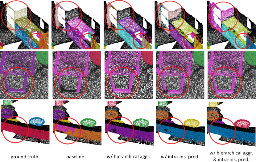
Figure 6: Qualitative results of challenging cases of ScanNet v2 [6]. Key regions are circled with red. The hierarchical aggregation and intra-instance prediction contribute to more fine-grained predictions, especially for objects with large sizes and fragmentary point clouds.

4.2 Quantitative Evaluation

ScanNet v2

In Tab. 1, we compare our HAIS with other methods on the unreleased testing set of ScanNet v2 [6] benchmark. HAIS achieves the highest $AP_{50}$ of $69.9\%$, ranking the first place on the leaderboard of ScanNet v2 and surpassing the previous state-of-the-art (SOTA) work [28] by $6.1\%$. For results on each class, our method achieves the best performance in $12$ out of $18$ classes.

S3DIS

In Tab. 2, we present the results on S3DIS. HAIS achieves much higher results than other methods in terms of all the widely-used metrics (mCov, mWCov, mPre and mRec). ScanNet v2 and S3DIS are quite different in terms of category, scene style and point cloud density. The SOTA performances of HAIS on both ScanNet v2 and S3DIS prove the high generalization ability.

4.3 Qualitative Evaluation

Fig. 6 visually shows the effectiveness of the hierarchical aggregation and intra-instance prediction. For objects with large sizes and fragmentary point clouds, grouping all points together is quite challenging. We can observe that with the proposed hierarchical aggregation and intra-instance prediction, precise instance segmentation masks are obtained.

4.4 Ablation Study

To validate the design of HAIS, we perform a series of ablation studies on the ScanNet validation set.

Ablation on the Hierarchical Aggregation and Intra-instance Prediction Network

Tab. 3 proves the effectiveness of the hierarchical aggregation and intra-instance prediction network. The intra-instance prediction promotes results by $2.7\%\ AP$, $2.4\%\ AP_{50}$ and $0.3\%\ AP_{25}$ . And the set aggregation further improves results by $1.0\%\ AP$, $0.7\%\ AP_{50}$ and $0.7\%\ AP_{25}$.

Point aggr.	Set aggr.	Intra-ins. pred.	$AP$	$AP_{50}$	$AP_{25}$
✓			39.8	61.0	74.6
✓		✓	42.5	63.4	74.9
✓	✓	✓	43.5	64.1	75.6

Table 3: Ablation results on the ScanNet v2 validation set. The hierarchical aggregation and intra-instance prediction bring significant gains in terms of $AP$, $AP_{50}$ and $AP_{25}$.

Using masks to filter points and calculate IoU	$AP$	$AP_{50}$	$AP_{25}$
	41.9	63.1	74.9
✓	43.5	64.1	75.6

Table 4: Ablation results on ScanNet v2 validation set for evaluating the effectiveness of using masks to filter points and calculate IoU.

Mask training samples	$AP$	$AP_{50}$	$AP_{25}$
All	42.8	63.3	74.4
IoU > 0.5	43.5	64.1	75.6

Table 5: Ablation results on ScanNet v2 validation set for evaluating the effectiveness of filtering mask training samples.

Method	Whole val set inference time (sec)	Per-frame inference time (msec)
SGPN [41]	49433	158439
ASIS [42]	56757	181913
GSPN [44]	3963	12702
3D-SIS [17]	38841	124490
3D-BoNet [43]	2871	9202
OccuSeg [15]	594	1904
PointGroup [20]	141	452
GICN [28]	2688	8615
HAIS	128	410

Table 6: The inference time on the validation set of ScanNet v2. For fair comparison, the inference time is measured on the same type of GPU (Titan X). Our HAIS achieves much better inference speed than other methods.

Using Masks to Filter Points and Calculate IoU

In the intra-instance prediction network, masks are used to assist certainty score predictions, i.e., filtering out features of background and calculating IoU which is the supervision signal of the instance certainty, as shown in Fig. 5. An alternative method is directly using the whole instance features without filtering background points to predict scores and using the IoU between the original input instance and the GT to supervise the instance certainty. Ablation experiments in Tab. 4 show that, using masks to filter points and calculate IoU improves the results. Filtering features with the mask can avoid the influence of the background noise. And masks are much more accurate than original input instances. The IoU between the mask and GT is more suitable to be the supervision signal of the certainty score.

Filtering Mask Training Samples

As shown in Tab. 5, compared with using all the instances as mask training samples, it’s better to filter out low quality instances with the IoU threshold of $0.5$. Low quality instances usually covers few foreground points but a large amount of background points. These instances may bring ambiguity to the instance-level refinement. It’s beneficial to filter them out during training.

4.5 Inference Speed

For real-life applications, e.g., mixed reality and autonomous driving, the inference speed of the whole network is of critical importance. We evaluate the efficiency of HAIS and compare it with other methods, as shown in Tab. 6. The single scene inference time is highly correlated to the number of points in the point cloud and varies a lot. Following the evaluation method of [43, 15, 28], we use the whole validation set inference time of ScanNet v2 for fair comparison on the efficiency. HAIS only takes $128$ seconds to infer all the 312 scans in the validation set, achieving the highest efficiency among all methods. On average, per scan inference latency of HAIS is $410$ ms. Point-wise prediction network, point aggregation, set aggregation and the intra-instance prediction network takes $172$, $125$, $4$, $109$ ms, respectively.

5 Conclusion

We propose HAIS, a concise bottom-up approach for 3D instance segmentation. We introduce the hierarchical aggregation to generate instance predictions in a two-step manner and the intra-instance prediction for more fine-grained instance predictions. Experiments on ScanNet v2 and S3DIS demonstrate the effectiveness and generalization of our method. HAIS also retains much better inference speed than all existing methods, showing its practicability in most scenarios, especially latency-sensitive ones.

Acknowledgement: This work was in part supported by NSFC (No. 61876212 and No. 61733007) and the Zhejiang Laboratory under Grant 2019NB0AB02.

In this supplementary material, we provide the detailed inference latency of main individual components of HAIS and compare it with other methods. Besides, we provide more qualitative results to demonstrate the effectiveness of HAIS.

Appendix A Detailed Inference Time

Tab. LABEL:tab:infer_detail shows the inference time of main components of different methods. Compared with other methods which require time-consuming clustering and post processing procedures, our HAIS keeps a much more efficient pipeline. The point-wise prediction network, point aggregation, set aggregation and intra-instance prediction network takes 172, 125, 4 and 109 ms, respectively.

Table 7: Inference time of main components of different methods on the ScanNet v2 validation set. For fair comparison, data in this table is measured on the same type of GPU (Titan X).

Method	Component inference time (msec)	Per frame inference time (msec)
SGPN [41]	backbone (GPU): 2080 group merging (CPU): 149000 block merging (CPU): 7119	158439
ASIS [42]	backbone (GPU): 2083 mean shift (CPU): 172711 block merging (CPU): 7119	181913
GSPN [44]	backbone (GPU): 1612 point sampling (GPU): 9559 neighbour search (CPU): 1500	12702
3D-BoNet [43]	backbone (GPU): 2083 SCN (GPU): 667 block merging (CPU): 7119	9202
OccuSeg [15]	backbone GPU): 189 supervoxel (CPU): 1202 clustering (GPU+CPU): 513	1904
PointGroup [20]	backbone (GPU): 128 clustering (GPU+CPU):221 ScoreNet (GPU): 103	452
GICN [28]	backbone (GPU): 1497 SCN (GPU): 667 block merging(CPU): 7119	8615
HAIS	point-wise prediction(GPU): 172 point aggregation(GPU+CPU): 125 set aggregation(GPU): 4 intra-instance prediction(GPU): 109	410

Appendix B Additional Qualitative Results

We show more qualitative results on the validation split of the ScanNet v2 dataset in Fig. 7. The predicted center shift vectors of some points are not accurate and a large amount of instance fragments come into being. By introducing the hierarchical aggregation and intra-instance prediction, HAIS generates fine-grained instance predictions.

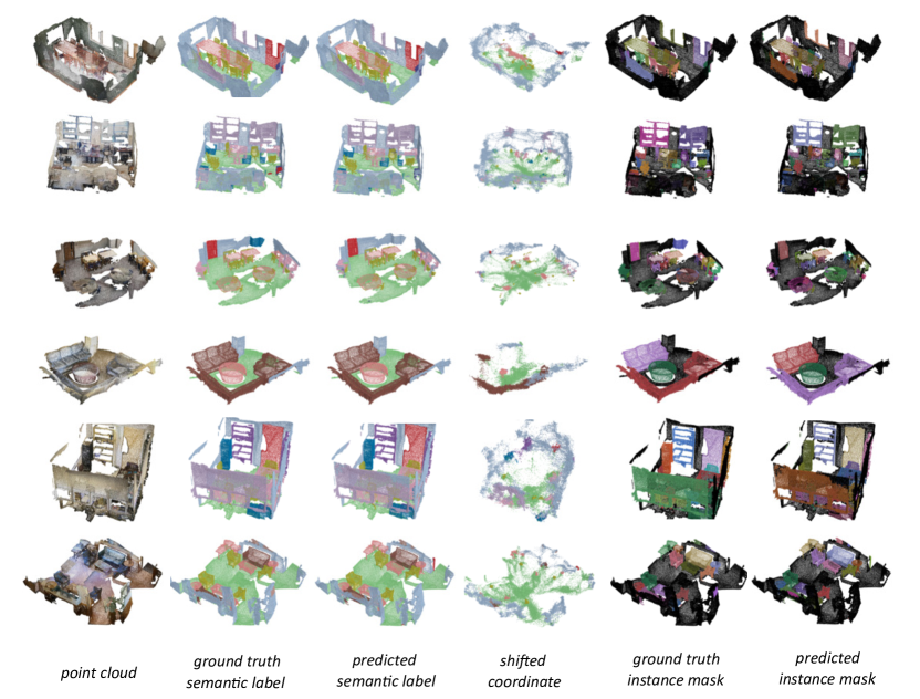
Figure 7: Qualitative results on ScanNet v2 [6]. From left to right: input point cloud, ground truth semantic label, predicted semantic label, shifted coordinate, ground truth instance mask and predicted instance mask. Best viewed in color.

References

- [1] Iro Armeni, Ozan Sener, Amir Roshan Zamir, Helen Jiang, Ioannis K. Brilakis, Martin Fischer, and Silvio Savarese. 3d semantic parsing of large-scale indoor spaces. In CVPR, 2016.
- [2] Min Bai and Raquel Urtasun. Deep watershed transform for instance segmentation. In CVPR, 2017.
- [3] Bert De Brabandere, Davy Neven, and Luc Van Gool. Semantic instance segmentation with a discriminative loss function. arXiv:1708.02551, 2017.
- [4] Kai Chen, Jiangmiao Pang, Jiaqi Wang, Yu Xiong, Xiaoxiao Li, Shuyang Sun, Wansen Feng, Ziwei Liu, Jianping Shi, Wanli Ouyang, Chen Change Loy, and Dahua Lin. Hybrid task cascade for instance segmentation. In CVPR, 2019.
- [5] Tianheng Cheng, Xinggang Wang, Lichao Huang, and Wenyu Liu. Boundary-preserving mask R-CNN. In ECCV, 2020.
- [6] Angela Dai, Angel X. Chang, Manolis Savva, Maciej Halber, Thomas A. Funkhouser, and Matthias Nießner. Scannet: Richly-annotated 3d reconstructions of indoor scenes. In CVPR, 2017.
- [7] Jifeng Dai, Kaiming He, Yi Li, Shaoqing Ren, and Jian Sun. Instance-sensitive fully convolutional networks. In ECCV, 2016.
- [8] Jifeng Dai, Yi Li, Kaiming He, and Jian Sun. R-FCN: object detection via region-based fully convolutional networks. In NeurIPS, 2016.
- [9] Francis Engelmann, Martin Bokeloh, Alireza Fathi, Bastian Leibe, and Matthias Nießner. 3d-mpa: Multi-proposal aggregation for 3d semantic instance segmentation. In CVPR, 2020.
- [10] Francis Engelmann, Theodora Kontogianni, and Bastian Leibe. Dilated point convolutions: On the receptive field size of point convolutions on 3d point clouds. In ICRA, 2020.
- [11] Yuxin Fang, Shusheng Yang, Xinggang Wang, Yu Li, Chen Fang, Ying Shan, Bin Feng, and Wenyu Liu. Instances as queries. arXiv:2105.01928, 2021.
- [12] Alireza Fathi, Zbigniew Wojna, Vivek Rathod, Peng Wang, Hyun Oh Song, Sergio Guadarrama, and Kevin P. Murphy. Semantic instance segmentation via deep metric learning. arXiv:1703.10277, 2017.
- [13] Ross B. Girshick. Fast R-CNN. In ICCV, 2015.
- [14] Benjamin Graham, Martin Engelcke, and Laurens van der Maaten. 3d semantic segmentation with submanifold sparse convolutional networks. In CVPR, 2018.
- [15] Lei Han, Tian Zheng, Lan Xu, and Lu Fang. Occuseg: Occupancy-aware 3d instance segmentation. In CVPR, 2020.
- [16] Kaiming He, Georgia Gkioxari, Piotr Dollár, and Ross B. Girshick. Mask R-CNN. PAMI, 2020.
- [17] Ji Hou, Angela Dai, and Matthias Nießner. 3d-sis: 3d semantic instance segmentation of RGB-D scans. In CVPR, 2019.
- [18] Zhaojin Huang, Lichao Huang, Yongchao Gong, Chang Huang, and Xinggang Wang. Mask scoring R-CNN. In CVPR, 2019.
- [19] Borui Jiang, Ruixuan Luo, Jiayuan Mao, Tete Xiao, and Yuning Jiang. Acquisition of localization confidence for accurate object detection. In ECCV, 2018.
- [20] Li Jiang, Hengshuang Zhao, Shaoshuai Shi, Shu Liu, Chi-Wing Fu, and Jiaya Jia. Pointgroup: Dual-set point grouping for 3d instance segmentation. In CVPR, 2020.
- [21] Shu Kong and Charless C. Fowlkes. Recurrent pixel embedding for instance grouping. In CVPR, 2018.
- [22] Jean Lahoud, Bernard Ghanem, Martin R. Oswald, and Marc Pollefeys. 3d instance segmentation via multi-task metric learning. In ICCV, 2019.
- [23] Buyu Li, Wanli Ouyang, Lu Sheng, Xingyu Zeng, and Xiaogang Wang. GS3D: an efficient 3d object detection framework for autonomous driving. In CVPR, 2019.
- [24] Yi Li, Haozhi Qi, Jifeng Dai, Xiangyang Ji, and Yichen Wei. Fully convolutional instance-aware semantic segmentation. In CVPR, 2017.
- [25] Tsung-Yi Lin, Piotr Dollár, Ross B. Girshick, Kaiming He, Bharath Hariharan, and Serge J. Belongie. Feature pyramid networks for object detection. In CVPR, 2017.
- [26] Chen Liu and Yasutaka Furukawa. MASC: multi-scale affinity with sparse convolution for 3d instance segmentation. arXiv:1902.04478, 2019.
- [27] Shu Liu, Lu Qi, Haifang Qin, Jianping Shi, and Jiaya Jia. Path aggregation network for instance segmentation. In CVPR, 2018.
- [28] Shih-Hung Liu, Shang-Yi Yu, Shao-Chi Wu, Hwann-Tzong Chen, and Tyng-Luh Liu. Learning gaussian instance segmentation in point clouds. arXiv:2007.09860, 2020.
- [29] Ilya Loshchilov and Frank Hutter. SGDR: stochastic gradient descent with warm restarts. In ICLR, 2017.
- [30] Daniel Maturana and Sebastian A. Scherer. Voxnet: A 3d convolutional neural network for real-time object recognition. In IROS, 2015.
- [31] Kaichun Mo, Shilin Zhu, Angel X. Chang, Li Yi, Subarna Tripathi, Leonidas J. Guibas, and Hao Su. Partnet: A large-scale benchmark for fine-grained and hierarchical part-level 3d object understanding. In CVPR, 2019.
- [32] Gaku Narita, Takashi Seno, Tomoya Ishikawa, and Yohsuke Kaji. Panopticfusion: Online volumetric semantic mapping at the level of stuff and things. In IROS, 2019.
- [33] Davy Neven, Bert De Brabandere, Marc Proesmans, and Luc Van Gool. Instance segmentation by jointly optimizing spatial embeddings and clustering bandwidth. In CVPR, 2019.
- [34] Quang-Hieu Pham, Duc Thanh Nguyen, Binh-Son Hua, Gemma Roig, and Sai-Kit Yeung. JSIS3D: joint semantic-instance segmentation of 3d point clouds with multi-task pointwise networks and multi-value conditional random fields. In CVPR, 2019.
- [35] Charles Ruizhongtai Qi, Hao Su, Kaichun Mo, and Leonidas J. Guibas. Pointnet: Deep learning on point sets for 3d classification and segmentation. In CVPR, 2017.
- [36] Charles Ruizhongtai Qi, Li Yi, Hao Su, and Leonidas J. Guibas. Pointnet++: Deep hierarchical feature learning on point sets in a metric space. In NeurIPS, 2017.
- [37] Shaoqing Ren, Kaiming He, Ross B. Girshick, and Jian Sun. Faster R-CNN: towards real-time object detection with region proposal networks. PAMI, 2017.
- [38] Gernot Riegler, Ali Osman Ulusoy, and Andreas Geiger. Octnet: Learning deep 3d representations at high resolutions. In CVPR, 2017.
- [39] Olaf Ronneberger, Philipp Fischer, and Thomas Brox. U-net: Convolutional networks for biomedical image segmentation. In MICCAI, 2015.
- [40] Lyne P. Tchapmi, Christopher B. Choy, Iro Armeni, JunYoung Gwak, and Silvio Savarese. Segcloud: Semantic segmentation of 3d point clouds. In 3DV, 2017.
- [41] Weiyue Wang, Ronald Yu, Qiangui Huang, and Ulrich Neumann. SGPN: similarity group proposal network for 3d point cloud instance segmentation. In CVPR, 2018.
- [42] Xinlong Wang, Shu Liu, Xiaoyong Shen, Chunhua Shen, and Jiaya Jia. Associatively segmenting instances and semantics in point clouds. In CVPR, 2019.
- [43] Bo Yang, Jianan Wang, Ronald Clark, Qingyong Hu, Sen Wang, Andrew Markham, and Niki Trigoni. Learning object bounding boxes for 3d instance segmentation on point clouds. In NeurIPS, 2019.
- [44] Li Yi, Wang Zhao, He Wang, Minhyuk Sung, and Leonidas J. Guibas. GSPN: generative shape proposal network for 3d instance segmentation in point cloud. In CVPR, 2019.
- [45] Hui Ying, Zhaojin Huang, Shu Liu, Tianjia Shao, and Kun Zhou. Embedmask: Embedding coupling for one-stage instance segmentation. arXiv:1912.01954, 2019.