Efficient simulations of high-spin black holes with a new gauge

Abstract

We present a new choice of initial data for binary black hole simulations that significantly improves the efficiency of high-spin simulations. We use spherical Kerr-Schild coordinates, where the horizon of a rotating black hole is spherical, for each black hole. The superposed spherical Kerr-Schild initial data reduce the runtime by a factor of 2 compared to standard superposed Kerr-Schild for an intermediate resolution spin-0.99 binary-black-hole simulation. We also explore different variations of the gauge conditions imposed during the evolution, one of which produces an additional speed-up of 1.3.

I Introduction

The exciting era of gravitational wave astronomy started with the first detection of a gravitational wave (GW) in 2015 by the Laser Interferometer Gravitational-Wave Observatory (LIGO) [1, 2, 3, 4]. The event, named GW150914, was generated by a binary-black-hole (BBH) system. About 50 detections have been published so far [5, 6] and most of them were emitted by BBHs, including GW190521 [7], the first detection of an intermediate-mass black hole (BH).

GW detection requires accurate waveform templates to extract the astrophysical signal from the noisy data. While a full analytic solution of BBH evolution is not known, analytical approximations like the post-Newtonian method can generate approximate BBH waveforms [8]. However, such approximations fail to describe the strong-field regime as the black holes merge [8]. Numerical relativity is currently the only way to model the merger event and provide full inspiral-merger-ringdown waveforms. Comparison between these numerically informed waveforms and detected signals allows GW observatories to extract physical properties about compact objects [4, 9] and measure possible deviations from general relativity [10, 11, 12, 13].

Since the first stable BBH simulations in 2005 [14, 15, 16], numerical relativists have enlarged the parameter space of simulations to include higher spins and mass ratios [17, 18, 19, 20, 21, 22, 23, 24, 25]. Nowadays, for example, the SXS Collaboration has published BBH simulations of dimensionless spin magnitude up to 0.998 in its catalog [25]. Though all the BBH events published so far by LIGO and Virgo have effective spin smaller than 0.9 (within 90% credible intervals) [5, 6], spin is not constrained to lie in this range and there is evidence of nearly extremal-spin BHs in X-ray binaries [26, 27, 28, 29, 30]. Thus, we must have models of high-spin BBH GW events so they can be searched for in the detector data.

There are several interesting phenomena that can occur for a high-spin BBH and not for a non-spinning one. Two examples are the hangup effect [31] and the flip-flop effect [32]. The hangup effect describes how the merger is delayed or accelerated by spin-orbit coupling compared to a non-spinning BBH merger, while the flip-flop effect may reverse the spin direction of a progenitor BH by spin-spin coupling. Both effects can be exaggerated by near-extremal spins, and can only be further understood by simulations. Furthermore, high-spin simulations are needed for filling out the parameter space for surrogate models [33, 34, 35, 36] and effective-one-body models [37, 38, 39, 40]. A recent development among surrogate models is NRSur7dq4 (together with NRSur7dq4Remnant), which is trained with numerical simulations of spin up to 0.8 [41]. An instance of effective-one-body calibrations using simulations of spin up to 0.98 can be found in Ref. [42].

Unfortunately, high-spin simulations are very computationally expensive, and rapidly increase in cost as the spins are increased. For example, a 25-orbit spin-0.9 BBH simulation takes weeks to complete, while a 25-orbit spin-0.99 simulation takes months to complete. Thus, a more efficient method of performing the simulations is highly desirable. Our objective in this paper is to develop faster high-spin BBH simulations by changing gauge conditions.

All simulations in this paper were done using the spectral Einstein code (SpEC) [43]. SpEC uses the first-order generalized harmonic evolution system to simulate the spacetime [44]. Before evolving spacetime quantities, SpEC solves for the initial data for BBH evolution using the extended conformal thin-sandwich formalism [45, 46]. SpEC chooses the free data to be given by a Gaussian-weighted combination of two single BH analytic solutions [47]. A traditional choice for the single BH analytic solution is Kerr-Schild (KS), while more recently harmonic-Kerr has been used successfully [48]. Simulations starting with harmonic-Kerr initial data are up to 30% faster than ones starting with KS. However, the harmonic-Kerr initial data can only be solved for spins smaller than 0.7 [48]. Reference [49] extends harmonic-Kerr initial data to spin-0.9 BBH simulations by using a modified version of harmonic-Kerr, but the overall computational efficiency is not greatly improved compared to simulations using the KS initial data.

In this paper we develop and use several gauge conditions both in the initial data and in the evolution. We compare their stability, efficiency, and gravitational waveform output with the goal of making high-spin (dimensionless spin $\chi\geq 0.9$) simulations cheaper. Our most successful choice of initial data reduces the cost of $\chi=0.99$ aligned-spin simulations by nearly a factor of 2.

The rest of this paper is organized as follows: in Sec. II, we describe the numerical methods that are crucial in SpEC BBH simulations and fundamental in the following discussion of this paper. In Sec. III, we introduce spherical Kerr-Schild as a spherical version of KS and wide Kerr-Schild as a modification of spherical Kerr-Schild that increases the coordinate separation between the inner and outer horizons. We will also briefly discuss how we delay the transition from the initial data gauge to the evolution gauge. In Sec. IV, we implement these new configurations in single BH and BBH simulations, and analyze their effect on computational cost, constraint violations, waveforms, resolution, and apparent horizons. We finally summarize the results and consider future developments in Sec. V.

Here are some conventions used in this paper. (1) Unless specified, spin refers to the dimensionless spin $\chi$. Dimensionful spin refers to spin angular momentum per unit mass and is labeled by $a$. (2) We use geometric units, i.e. $G=c=1$. All dimensionful quantities in this paper are then equipped with units that are an integer power of $M$, the total ADM mass of a system. For example, time and distance have units of $M$. (3) We use letters at the beginning of the Latin alphabet ($a,b,c,\dots$) as spacetime indices, and later letters ($i,j,k,\dots$) as spatial indices. (4) We reserve symbols $g_{ab}$, $\gamma_{ij}$, $\alpha$, and $\beta^{i}$ for spacetime metric, spatial metric, lapse, and shift.

II Numerical techniques

In this section, we provide an overview of some of the numerical methods SpEC uses. We start by briefly describing the extended conformal thin-sandwich formalism and SpEC’s choice of free data in Sec. II.1. Next, we discuss the first-order generalized harmonic system in Sec. II.2. Finally, in Sec. II.3, we briefly describe the configuration of the computational domain in SpEC.

II.1 Binary-black-hole initial data

We adopt the standard 3+1 form of the spacetime metric $g_{ab}$,

$$ds^{2}=-\alpha^{2}\,dt^{2}+\gamma_{ij}\left(\beta^{i}\,dt+dx^{i}\right)\left(\beta^{j}\,dt+dx^{j}\right),$$ (1)

where $\alpha$ is the lapse, $\beta^{i}$ the shift, and $\gamma_{ij}$ the spatial metric. In vacuum, the spacetime metric $g_{ab}$ and its time derivative $\partial_{t}g_{ab}$ must satisfy the Hamiltonian and momentum constraints,

$$R+K^{2}-K_{ij}K^{ij} =0,$$ (2)

$$D_{j}(K^{ij}-\gamma^{ij}K) =0,$$ (3)

where $R$ is the spatial Ricci scalar, $D_{i}$ the spatial covariant derivative, $K_{ij}$ the extrinsic curvature, and $K=K^{i}{}_{i}$ the trace of the extrinsic curvature.

The spatial metric and extrinsic curvature are split using a conformal decomposition as

$$\gamma_{ij} =\psi^{4}\bar{\gamma}_{ij},$$ (4)

$$K_{ij} =A_{ij}+\frac{1}{3}\gamma_{ij}K,$$ (5)

where $\psi$ is the conformal factor, $\bar{\gamma}_{ij}$ the conformal metric, and $A_{ij}$ the traceless part of $K_{ij}$. $A_{ij}$ is further decomposed as

$$A_{ij} =\psi^{-2}\bar{A}_{ij},$$ (6)

$$\bar{A}^{ij} =\frac{\psi^{6}}{2\alpha}\left((\bar{L}\beta)^{ij}-\bar{u}^{ij}\right),$$ (7)

where $\bar{u}_{ij}\equiv\partial_{t}\bar{\gamma}_{ij}$ (note that $\bar{\gamma}^{ij}\bar{u}_{ij}=0$ to uniquely fix $\bar{u}_{ij}$ [50]), and the vector gradient part $(\bar{L}\beta)^{ij}$ is defined as

$$(\bar{L}\beta)^{ij}\equiv\bar{D}^{i}\beta^{j}+\bar{D}^{j}\beta^{i}-\frac{2}{3}\bar{\gamma}^{ij}\bar{D}_{k}\beta^{k},$$ (8)

with $\bar{D}_{j}$ the covariant derivative associated with $\bar{\gamma}_{ij}$.

In the extended conformal thin-sandwich formalism, $\bar{\gamma}_{ij}$, $\bar{u}_{ij}$, $K$, and $\partial_{t}K$ are freely specifiable. The elliptic solver in SpEC [51] computes $\psi$, $\alpha$, and $\beta^{i}$ by solving

$$\bar{D}_{j}\left(\frac{\psi^{6}}{2\alpha}(\bar{L}\beta)^{ij}\right)-\bar{D}_{j}\left(\frac{\psi^{6}}{2\alpha}\bar{u}^{ij}\right)-\frac{2}{3}\psi^{6}\bar{D}^{i}K=0,$$ (9)

$$\bar{D}^{2}\psi-\frac{1}{8}\psi\bar{R}-\frac{1}{12}\psi^{5}K^{2}+\frac{1}{8}\psi^{-7}\bar{A}_{ij}\bar{A}^{ij}=0,$$ (10)

$$\bar{D}^{2}(\alpha\psi)-\alpha\psi\left(\frac{7}{8}\psi^{-8}\bar{A}_{ij}\bar{A}^{ij}+\frac{5}{12}\psi^{4}K^{2}+\frac{1}{8}\bar{R}\right)$$

$$\hskip 33.96698pt+\psi^{5}(\partial_{t}K-\beta^{k}\partial_{k}K)=0,$$ (11)

where $\bar{R}$ is the conformal Ricci scalar. Equations (4) and (5) are then used to compute $\gamma_{ij}$ and $K_{ij}$.

The free variables $\bar{u}_{ij}$ and $\partial_{t}K$ are typically set to 0 to construct quasi-equilibrium initial data. SpEC sets the remaining free variables $\bar{\gamma}_{ij}$ and $K$ using a superposition of two single BH spacetimes blended together by a Gaussian weight function [47]. We define $\gamma^{\rho}_{ij}$ and $K^{\rho}$ to refer to these quantities for a boosted spinning BH, where $\rho=A,B$ labels each BH. $\bar{\gamma}_{ij}$ and $K$ are chosen to be [47]

$$\bar{\gamma}_{ij} \equiv\eta_{ij}+\sum_{\rho}e^{-r^{2}_{\rho}/w^{2}_{\rho}}(\gamma^{\rho}_{ij}-\eta_{ij}),$$ (12)

$$K \equiv\sum_{\rho}e^{-r^{2}_{\rho}/w^{2}_{\rho}}K^{\rho},$$ (13)

where $\eta_{ij}$ is the 3D flat metric, $r_{\rho}$ is the Euclidean distance from BH $\rho$, and $w_{\rho}$ controls the falloff of BH $\rho$’s contribution. We use $w_{\rho}$ equal to 3/5 of the Euclidean distance between the BBH’s L1 Lagrange point (Euclidean center-of-mass) and BH $\rho$’s center. This choice of $w_{\rho}$ is wider than a BH’s size but still relatively far from the companion BH.

The most common choice for the free data at each BH is Kerr-Schild (KS), though using harmonic-Kerr has much promise for low-spin binaries [48]. In this paper, we use a Kerr-Schild-like gauge where the horizon is spherical at each black hole to set the free data. We will discuss the KS and KS-like gauges in Sec. III.

II.2 Generalized harmonic evolution system

SpEC evolves the initial data using the first-order generalized harmonic (GH) system [44]. (See Refs. [52, 53, 54] for more details on the GH systems.) The coordinates $x^{a}$ (referred to as generalized harmonic coordinates) satisfy the inhomogeneous wave equation,

$$H^{a}=\nabla_{b}\nabla^{b}x^{a}=-\Gamma^{a},$$ (14)

where $\Gamma^{a}\equiv g^{bc}\Gamma^{a}_{bc}$ is the trace of the Christoffel symbol, and $\nabla_{a}$ the $g_{ab}$-compatible covariant derivative. The gauge source function $H^{a}=H^{a}(x^{b},g_{cd})$ is any arbitrary function dependent only on $x^{b}$ and $g_{cd}$ (but not derivatives of $g_{ab}$). In these coordinates, the vacuum Einstein equations can be cast into a manifestly hyperbolic form,

$$g^{cd}\partial_{c}\partial_{d}g_{ab}= -2\nabla_{(a}H_{b)}$$

$$+2g^{cd}g^{ef}(\partial_{e}g_{ca}\partial_{f}g_{db}-\Gamma_{ace}\Gamma_{bdf}),$$ (15)

where $\Gamma_{abc}=g_{ad}\Gamma^{d}_{bc}$. After expanding Eq. (15) into a first-order representation (done analogously to expanding the covariant scalar field system [55, 56]) and adding constraint damping terms (see [57, 54, 58, 14, 44] for detailed discussions on constraint damping), we arrive at the GH evolution equations implemented in SpEC,

$$\partial_{t}g_{ab} =-\alpha\Pi_{ab}-\gamma_{1}\beta^{i}\Phi_{iab}+\left(1+\gamma_{1}\right)\beta^{k}\partial_{k}g_{ab},$$ (16)

$$\partial_{t}\Pi_{ab} =2\alpha g^{cd}\left(g^{ij}\Phi_{ica}\Phi_{jdb}-\Pi_{ca}\Pi_{db}-g^{ef}\Gamma_{ace}\Gamma_{bdf}\right)$$

$$-2\alpha\nabla_{(a}H_{b)}-\frac{1}{2}\alpha n^{c}n^{d}\Pi_{cd}\Pi_{ab}-\alpha n^{c}\Pi_{ci}g^{ij}\Phi_{jab}$$

$$+\alpha\gamma_{0}\left[2\delta^{c}{}_{(a}n_{b)}-(1+\gamma_{3})g_{ab}n^{c}\right]\left(H_{c}+\Gamma_{c}\right)$$

$$-\gamma_{1}\gamma_{2}\beta^{i}\Phi_{iab}+\beta^{k}\partial_{k}\Pi_{ab}-\alpha g^{ki}\partial_{k}\Phi_{iab}$$

$$+\gamma_{1}\gamma_{2}\beta^{k}\partial_{k}g_{ab},$$ (17)

$$\partial_{t}\Phi_{iab} =\frac{1}{2}\alpha n^{c}n^{d}\Phi_{icd}\Pi_{ab}+\alpha g^{jk}n^{c}\Phi_{ijc}\Phi_{kab}-\alpha\gamma_{2}\Phi_{iab}$$

$$+\beta^{k}\partial_{k}\Phi_{iab}-\alpha\partial_{i}\Pi_{ab}+\alpha\gamma_{2}\partial_{i}g_{ab},$$ (18)

where $g_{ab}$, $\Phi_{iab}\equiv\partial_{i}g_{ab}$, $\Pi_{ab}\equiv-n^{c}\partial_{c}g_{ab}$ are the three dynamical fields being evolved, $\gamma_{0}$, $\gamma_{1}$, $\gamma_{2}$ and $\gamma_{3}$ the constraint damping parameters, and $n^{a}$ the future-pointing unit normal to constant-$t$ spatial hypersurfaces. See the Appendix for values of $\gamma_{0}$, $\gamma_{1}$, $\gamma_{2}$ and $\gamma_{3}$ used in the simulations of this paper.

The simplest choice of gauge source function is the harmonic gauge, where $H^{a}=0$. The harmonic gauge dates back to Einstein’s work [59] and has been an important tool in many aspects of analytical general relativity [60, 61, 62]. Unfortunately, using a harmonic gauge condition in simulations of BBH mergers leads to explosive growth of $\gamma=\det(\gamma_{ij})$ near the apparent horizons as two BHs merge [63]. To suppress such growth, SpEC adopts the damped wave gauge or damped harmonic (DH) gauge $H^{a}=H^{a}_{\text{DH}}$ [63],

$$H^{a}_{\text{DH}}=\mu_{L}n^{a}\ln\left(\frac{\sqrt{\gamma}}{\alpha}\right)-\mu_{S}\frac{\beta^{i}}{\alpha}\gamma^{a}_{\ i},$$ (19)

$$\mu_{L}=\mu_{S}=e^{-(\ln 10^{15})r^{2}/\sigma^{2}}\left[\ln\left(\frac{\sqrt{\gamma}}{\alpha}\right)\right]^{2},$$ (20)

where $r$ is the Euclidean radius, and $\sigma=100M$. Note that the DH gauge reduces to the harmonic gauge to machine precision for $r\geq\sigma$.

SpEC uses the following gauge transition from the initial gauge $H_{\text{init}}^{a}$ to the DH gauge $H^{a}_{\text{DH}}$ during evolution:

$$H^{a}=F(t)H^{a}_{\mathrm{init}}+\left[1-F(t)\right]H^{a}_{\mathrm{DH}},$$ (21)

where

$$F(t)=\begin{dcases}\exp\left[-\left(\frac{t-t_{0}}{w}\right)^{4}\right],&t\geq t_{0}\\ 1,&t<t_{0}.\end{dcases}$$ (22)

Here $t_{0}$ is the start time and $w$ is the temporal width of the transition. Unless stated otherwise, we choose $t_{0}=0M$ and $w=50M$. Note that this transition function is not finely tuned. It is chosen because it decays to 0 rapidly for large $t$ and has a continuous third derivative at $t=t_{0}$.

II.3 Computational domain

SpEC adopts a dual-frame configuration for BBH simulations [64]. In the inertial frame, the two BHs are orbiting each other and deform as they merge. In contrast, in the grid frame, the BHs are at fixed coordinate locations and are kept approximately spherical. The two frames are related by a time-dependent analytic map determined by feedback control systems in SpEC [65].

SpEC’s domain decomposition is described in the Appendix of Ref. [66], while the adaptive mesh refinement (AMR) algorithm is described in Refs. [67, 68]. SpEC uses spherical shells around each BH. The number of spherical harmonic modes ($\ell$) used in the shells around BHs is a direct proxy for how the shape of each BH affects the computational cost of a simulation. High-spin BBH simulations use $\ell\geq 40$, which results in not only many grid points, but also close spacing between grid points. A simulation with more grid points requires more computation per time step, while a closer spacing between grid points requires a smaller time step in order to maintain stability. Both factors slow down the overall simulation. With this in mind, we seek to reduce the angular resolution needed in high-spin BBH simulations, anticipating faster simulations.

SpEC uses excision to avoid the physical singularities inside BHs. Specifically, the region within an inner boundary for each BH is excluded from the computational domain. This boundary is called an excision surface or excision boundary and lies slightly inside the apparent horizon (AH) of each BH [54, 65]. Causality prohibits any physical content in the interior region from propagating out. The excision surface has to be placed in a trapped region between the inner and outer horizons for each BH. Since the distance between the inner and outer horizons decreases as spin increases, the placement of the excision boundary becomes increasingly difficult as the spin increases. As a result, smaller time step sizes are necessary to track the apparent horizons and to keep the excision boundary inside the narrow trapped region. Thus, a gauge where horizons remain spherical for any spin should not only decrease the resolution used by AMR but also reduce the workload in tracking the apparent horizons and controlling the excision boundaries. At the outer boundary, suitable constraint-preserving boundary conditions [44] are imposed.

III New initial data and gauge conditions

We describe three modifications to SpEC’s current configuration that will be explored in this paper. The major modification is to introduce a Kerr-Schild-like gauge in the free initial data, where the horizons are spherical for any spin. We will refer to this choice as spherical Kerr-Schild. The other two modifications are variants of the spherical KS initial data. One variant increases the coordinate distance between the inner and outer horizons in spherical Kerr-Schild to construct what we refer to as the wide Kerr-Schild gauge. The other variant keeps the spherical Kerr-Schild data, but delays the transition to damped harmonic gauge during the evolution.

III.1 Spherical Kerr-Schild

The Kerr metric in KS coordinates $\{t,x,y,z\}$, with spin pointing along the $z$-axis, mass $M$, and angular momentum $aM=\chi M^{2}$ is

$$g_{ab}=\eta_{ab}+2Hl_{a}l_{b},$$ (23)

where $\eta_{ab}$ is the Minkowski metric,

$$H =\frac{Mr^{3}}{r^{4}+a^{2}z^{2}},$$ (24)

$$l_{a} =\left(1,\frac{rx+ay}{r^{2}+a^{2}},\frac{ry-ax}{r^{2}+a^{2}},\frac{z}{r}\right),$$ (25)

and $r$ implicitly given by

$$\frac{x^{2}+y^{2}}{r^{2}+a^{2}}+\frac{z^{2}}{r^{2}}=1$$ (26)

is the radial coordinate in Boyer-Lindquist coordinates. Since we are only interested in astrophysical BHs, we restrict ourselves to $\chi<1$. Then for any nonzero spin, there are inner and outer horizons $r_{\pm}=(1\pm\sqrt{1-\chi^{2}})M$. In the region $r_{-}<r<r_{+}$, any object must travel radially inward, while outside this region ($r<r_{-}$ or $r>r_{+}$, excluding horizons), an object can travel both radially inward and outward. For high spins, the horizons $r_{\pm}$ become closer together and increasingly non-spherical in the KS coordinate system, requiring greater angular resolution to simulate the BHs. This suggests that we might mitigate the required resolution increase by using coordinates in which the horizons are spherical, as we now describe.

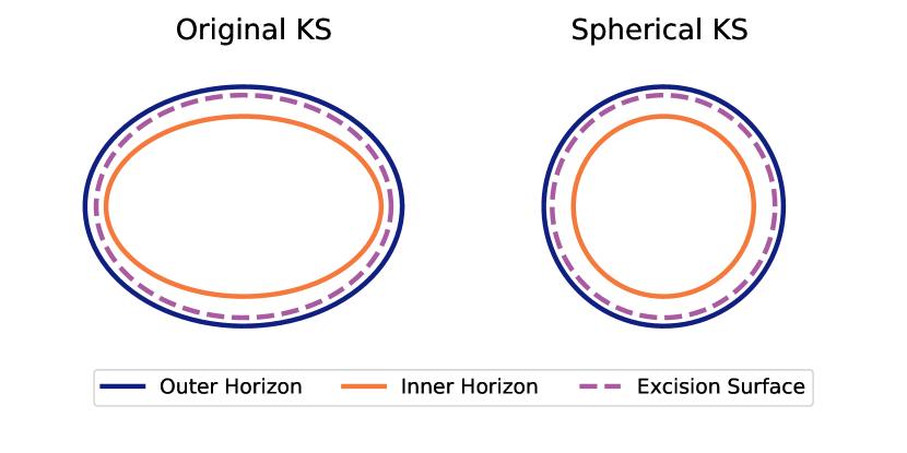
Figure 1: The $xz$-plane for a single BH with spin 0.9 along the $z$-axis in KS coordinates (left) and spherical KS coordinates (right). The left diagram shows that the excision surface and both horizons are spheroids. The right one shows that in spherical KS coordinates the excision surface and horizons are spheres.

We denote the spherical KS coordinates by $\{t,\bar{x},\bar{y},\bar{z}\}$. These are related to the KS coordinates $\{t,x,y,z\}$ by

$$\frac{\bar{x}}{r} =\frac{x}{\sqrt{r^{2}+a^{2}}},$$ (27)

$$\frac{\bar{y}}{r} =\frac{y}{\sqrt{r^{2}+a^{2}}},$$ (28)

$$\bar{z} =z.$$ (29)

Equation (26) describes an oblate spheroid in $\{x,y,z\}$ and is equivalent to a sphere in $\{\bar{x},\bar{y},\bar{z}\}$ coordinates. That is,

$$\bar{x}^{2}+\bar{y}^{2}+\bar{z}^{2}=r^{2}.$$ (30)

The left panel of Fig. 1 shows the inner and outer horizons in KS as solid lines, and a sample excision surface as a dashed line. The right panel of Fig. 1 shows the inner and outer horizons, and excision surface but in spherical KS coordinates instead. We will abbreviate spherical KS as SphKS hereinafter.

III.2 Wide Kerr-Schild

Recall from Sec. II.3 that as the BHs inspiral, the excision regions track the BHs. The excision boundary must be inside $r_{+}$ but outside $r_{-}$ so that all information leaves the computational domain and no boundary condition must be applied. This becomes more difficult as the spin increases, partly because the space between $r_{+}$ and $r_{-}$ decreases. We attempt to reduce the work of the control system by expanding the region between the horizons by performing a radial transformation. Note that the idea of expanding the region between horizons in the initial data is not new. For example, Ref. [69] applies a fisheye radial transformation to the quasi-isotropic coordinates to expand the horizon size. We here apply a different radial transformation to the SphKS coordinates. We refer to this gauge as wide Kerr-Schild (WKS). We continue using the notation in Sec. III.1 and denote the coordinates of WKS as {$t,\tilde{x},\tilde{y},\tilde{z}$}. We introduce a new variable $\tilde{r}$ that is related to $r$ and choose the coordinate transformation between WKS and SphKS as

$$\frac{\tilde{x}}{\tilde{r}} =\frac{\bar{x}}{r},$$ (31)

$$\frac{\tilde{y}}{\tilde{r}} =\frac{\bar{y}}{r},$$ (32)

$$\frac{\tilde{z}}{\tilde{r}} =\frac{\bar{z}}{r}.$$ (33)

With this convention, Eqs. (26) and (30) are equivalent to

$$\tilde{x}^{2}+\tilde{y}^{2}+\tilde{z}^{2}=\tilde{r}^{2},$$ (34)

i.e. a sphere of radius $\tilde{r}$ in WKS.

Starting with SphKS, we want a radial transformation $r\rightarrow\tilde{r}$ that keeps $r_{+}$ fixed but shrinks $r_{-}$ radially inward by some factor $b$, i.e.,

$$\tilde{r}(r_{+}) =r_{+},$$ (35)

$$\tilde{r}(r_{-}) =br_{-}.$$ (36)

We can achieve these relations with a quadratic,

$$\tilde{r}(r)=\frac{1-b}{r_{+}-r_{-}}r^{2}+\frac{br_{+}-r_{-}}{r_{+}-r_{-}}r,$$ (37)

with $r_{-}/r_{+}\leq b\leq 1$ to ensure monotonicity, e.g., the lower bound of $b$ is $\sim 0.75$ for a spin-0.99 BH. This $b$ is a squeezing parameter that controls how far $r_{-}$ is pushed inwards after the transformation.

Unfortunately, this quadratic has the pathology that the metric would no longer be asymptotically flat, so we use the quadratic only near the BH, smoothly transitioning to $\tilde{r}=r$ far away from the BH. Specifically,

$$r(\tilde{r})=\frac{\sqrt{B^{2}+4A\tilde{r}}-B-2A\tilde{r}}{2A}\frac{1}{1+e^{(\tilde{r}-C)/\lambda}}+\tilde{r},$$ (38)

where

$$A =\frac{1-b}{r_{+}-r_{-}},$$ (39)

$$B =\frac{br_{+}-r_{-}}{r_{+}-r_{-}}=1-Ar_{+}.$$ (40)

We write the relation as a function $r(\tilde{r})$ instead of $\tilde{r}(r)$ for easier implementation in SpEC. $C$ and $\lambda$ are parameters of the sigmoid function, controlling the center and width of transition. Theoretically, we could choose $C$ and $\lambda$ to satisfy $e^{(r_{+}-C)/\lambda}\sim 10^{-15}$ so that Eq. (37) holds exactly inside $r_{+}$ within numerical precision, but such combinations always result in large Jacobians. A quantity with large derivatives (and second derivatives) needs sufficiently high resolution to be resolved, which increases computational cost. In practice, because the starting point of WKS is broadening the region between $r_{+}$ and $r_{-}$ nonlinearly, we simply choose $C=3M$ and $\lambda=8M$. This combination of $C$ and $\lambda$ maintains stable simulations without increasing computational cost too much. Figure 2 shows $\tilde{r}/r$ versus $r$ for these $C$ and $\lambda$.

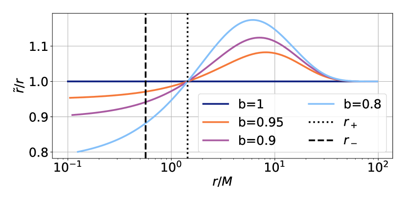
Figure 2: The ratio $\tilde{r}/r$ as a function of $r$ for various squeezing parameters $b$ for a spin-0.9 BH with $C=3M$ and $\lambda=8M$. The horizontal axis ($r/M$) is on a logarithmic scale to show both near-field and far-field behaviors. Since for $b=1$ (no squeezing) $\tilde{r}=r$, the curve stays at 1. All curves tend to 1 far from the BH to preserve asymptotic flatness, while becoming smaller than 1 inside the outer horizon. The reader can confirm from the graph that the transformation in Eq. (38) keeps $r_{+}$ fixed.

III.3 Delayed evolution gauge transition

When studying evolutions using SphKS initial data we noticed that the apparent horizons become spheroids around $t=50M$ when the gauge has mostly transitioned to damped harmonic. With the change to a spheroidal horizon we observe the expected increase in the required angular resolution. Since the damped harmonic (DH) condition is generally only necessary during merger, we perform simulations where we delay the transition from $H^{a}_{\mathrm{init}}$ to $H^{a}_{\mathrm{DH}}$ in an attempt to extend how long the horizons remain (nearly) spherical. We change both $t_{0}$ and $w$ in Eq. (22) and report our results in Sec. IV.5.

IV Results

In this section, we test the new configurations described in Sec. III by evolving multiple single BH and BBH systems. In particular, we will compare the constraint violations, computational efficiency, AH shapes, total number of grid points, and waveforms from different simulations.

IV.1 Single spherical Kerr-Schild black hole

We evolve a spin-0.99 BH to time $4000M$ in both KS and SphKS coordinates. We keep the domain decomposition the same by using the transformation Eqs. (27$-$29) from the SphKS domain, such that any sphere is mapped to a spheroid matching the given spin. AMR is disabled, ensuring the domain decomposition and resolution are unchanged throughout the simulations. We fix the radial resolution in both coordinates but vary the angular resolutions, represented by $\ell$. The number of angular grid points is then $2(\ell+1)^{2}$. We investigate four single BH simulations: three in KS with $\ell=22,26,30$ and one in SphKS with $\ell=22$.

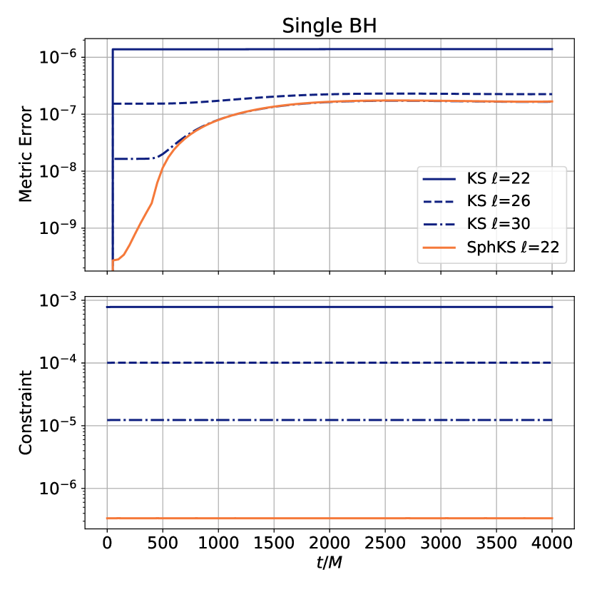
Figure 3: Metric errors and constraint energy of four single BH simulations. The top panel plots the $L_{2}$-norm of the error of the spacetime metric, i.e. the $L_{2}$-norm of $g_{ab}-g_{ab}^{\mathrm{analytic}}$. The bottom panel plots the $L_{2}$-norm of the constraint energy. The blue lines represent the simulations using KS initial data, with $\ell=22,26,30$ in the solid, dashed, and dash-dotted line styles, while the orange solid lines are results from the SphKS $\ell=22$ simulation. As $\ell$ increases, the KS simulations achieve lower metric errors and constraint violations. The SphKS $\ell=22$ simulation has lower metric errors and constraint violations than the KS $\ell=22$ case by factors of 10 and $10^{3}$. Note that the $10^{-7}$ error floor of the metric errors at late times is caused by the outer boundary condition.

In the top panel of Fig. 3, we show the $L_{2}$-norm of the metric errors $g_{ab}-g_{ab}^{\mathrm{analytic}}$ for all four simulations. The blue lines represent the evolution using KS coordinates, with $\ell=22,26,30$ corresponding to the solid, dashed and dash-dotted styles. The metric error decreases as the angular resolution increases, especially at early time (before $t<500M$). After $t\sim 1000M$, the metric error approaches a $10^{-7}$ error floor. This error floor appears because the numerical error gets reflected at the outer boundary and amplified when traveling inward [70]. The orange line is for the evolution using SphKS coordinates with $\ell=22$. It reaches the same error floor at late time but is at least 10 times smaller than the metric error of the $\ell=22$ KS simulation (the blue solid curve).

In the bottom panel of Fig. 3, we show the GH constraint energy $\mathcal{E}_{c}$ for these four simulations. The constraint energy (or constraint violation) used in this paper is defined as

$$\mathcal{E}_{c}=\displaystyle\sqrt{\frac{\int\mathcal{C}_{\mathrm{GH}}^{2}\sqrt{\gamma}d^{3}x}{\int\sqrt{\gamma}d^{3}x}},$$ (41)

where

$$\mathcal{C}_{\mathrm{GH}}^{2}=\delta^{ab} [\gamma^{ij}(\mathcal{C}_{ia}\mathcal{C}_{jb}+\delta^{cd}\mathcal{C}_{iac}\mathcal{C}_{jbd}+\gamma^{kl}\delta^{cd}\mathcal{C}_{ikac}\mathcal{C}_{jlbd})$$

$$+\mathcal{F}_{a}\mathcal{F}_{b}+\mathcal{C}_{a}\mathcal{C}_{b}].$$ (42)

Here, $\delta^{ab}$ is the 4D Kronecker delta and {$\mathcal{C}_{a}$, $\mathcal{F}_{a}$, $\mathcal{C}_{ia}$, $\mathcal{C}_{iab}$, $\mathcal{C}_{ijab}$} are the five constraints used in Ref. [44]. Note that our definition of $\mathcal{E}_{c}$ is different from the one in Ref. [44]. Among the simulations using KS coordinates, the constraint violation is smaller as $\ell$ increases. In contrast to the metric errors, the constraint violations do not hit an error floor because of the use of a constraint-preserving boundary condition [70]. We see that the SphKS evolution has constraint violation over a factor of $10^{3}$ smaller than the evolution in KS coordinates using the same angular resolution ($\ell=22$). Even compared to the KS $\ell=30$ case, the SphKS $\ell=22$ simulation still has a smaller constraint violation by a factor of 10.

Table 1: Parameters for the six BBH simulations studied in Secs. IV.2 and IV.3. $\vec{\chi}_{A,B}$ are the spin vectors of the progenitor-BHs. $D_{0}$, $\Omega_{0}$, $\dot{a}_{0}$ and $e$ are the initial coordinate separation, initial orbital frequency, initial rate of change of separation, and eccentricity. All these six simulations have mass ratio 1.

$\vec{\chi}_{A,B}$	Initial data gauge	$D_{0}$ $[M]$	$\Omega_{0}$	$\dot{a}_{0}$	$e$	# of orbits
(0, 0, 0.9)	KS	15.450	1.4095$\times 10^{-2}$	5.3578$\times 10^{-4}$	$\sim 0.0003$	$\sim 25$
	SphKS	15.450	1.42$\times 10^{-2}$	4.5284$\times 10^{-4}$	$\sim 0.0005$	$\sim 25$
(0, 0, 0.95)	KS	11.580	2.0875$\times 10^{-2}$	1.0650$\times 10^{-3}$	$\sim 0.0007$	$\sim 14$
	SphKS	11.580	2.1100$\times 10^{-2}$	8.5921$\times 10^{-4}$	$\sim 0.0005$	$\sim 14$
(0, 0, 0.99)	KS	11.577	2.0384$\times 10^{-2}$	1.4799$\times 10^{-3}$	$\sim 0.0005$	$\sim 14$
	SphKS	11.577	2.0808$\times 10^{-2}$	1.1357$\times 10^{-3}$	$\sim 0.0002$	$\sim 14$

Because the horizons are spherical in the SphKS gauge, spacetime quantities are constructed and evolved directly in spherical domains. In the KS gauge, quantities are evolved in spheroidal domains, so a spatial map converting spheroids to spheres is necessary in the spectral calculation of derivatives. The Jacobian and Hessian of this spatial map and its inverse can introduce errors. Thus, in Fig. 3, we see the single BH simulation in SphKS provides a more accurate result than in KS.

The KS $\ell=22$ simulation takes 978 CPU hours to reach $t=4000M$, while the SphKS $\ell=22$ simulation takes 948 CPU hours on the same number of cores. However, a better comparison is to the $\ell=26$ KS case, which takes 1438 CPU hours and still has considerably larger errors. It may not be surprising that we are able to reduce the numerical error of single BH simulations by using coordinates better adapted to the geometry of the BH, but it is reassuring to have confirmation.

IV.2 Spin-0.9 binary-black-hole simulations using spherical Kerr-Schild initial data

We evolve three pairs of non-eccentric, non-precessing, equal-mass, equal-spin BBH systems, corresponding to spin 0.9, 0.95, and 0.99, all along the $z$-axis. Each pair consists of a run with superposed KS initial data and another run with superposed SphKS initial data. They both merge after nearly the same number of orbits and at nearly the same simulation time. The initial orbital frequency $\Omega_{0}$ and the initial rate of change of separation $\dot{a}_{0}$ are tuned separately for each run, subject to a fixed initial separation $D_{0}$. We perform this tuning by eccentricity reduction [71] to achieve a negligible eccentricity $(e<0.0007)$. The specific values of these parameters, including the number of orbits, are provided in Table 1. Furthermore, we simulate each BBH run at three resolutions, Lev-1, Lev-2, and Lev-3. For Lev-$i$, the target truncation error of the AMR algorithm is $\sim 2\times 4^{-i}\times 10^{-4}$.

We focus on the spin-0.9 and spin-0.99 simulations in this paper. Comparisons of CPU times and constraint energy [Eq. (41)] between the two gauges for the spin-0.9 and spin-0.99 simulations are shown in Fig. 4. Comparison of waveforms for the spin-0.9 and spin-0.99 Lev-3 simulations are shown in Fig. 5. Additionally, the CPU times at the end of ringdown are recorded in Table 2. We will explain and analyze these figures and tables in greater detail.

We do not show figures for the spin-0.95 case because the spin-0.95 and spin-0.99 simulations share the same qualitative behavior. However, we still provide the CPU times of the spin-0.95 case in Table 2 to show the trend that using SphKS accelerates BBH simulations more significantly as the spin increases.

Table 2: CPU times at the end of the six BBH simulations. $T_{\text{KS}}$ and $T_{\text{SphKS}}$ are the CPU times with the KS and SphKS initial data. We calculate the ratio $T_{\text{SphKS}}/T_{\text{KS}}$ for each spin and Lev in the fifth column. A smaller ratio means the SphKS simulation is more efficient than the KS simulation. We see improvements in all cases. The CPU time ratio ranges from $\sim$0.56 to $\sim$0.93. In the two most expensive runs, spin-0.95 Lev-3 and spin-0.99 Lev-3 runs, using the SphKS initial data is almost 2 times faster than using the KS initial data.

Spin	Lev	$T_{\text{KS}}$ [hr]	$T_{\text{SphKS}}$ [hr]	$T_{\text{SphKS}}/T_{\text{KS}}$
0.9	1	10582	8307	0.785
	2	16957	14628	0.863
	3	23369	21272	0.910
0.95	1	7318	6778	0.926
	2	10273	9094	0.885
	3	22697	13104	0.577
0.99	1	14651	13147	0.897
	2	28764	18312	0.637
	3	70709	39583	0.560

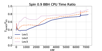
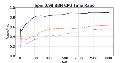
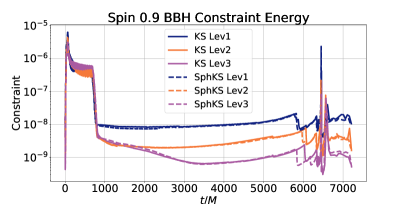
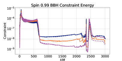
Figure 4: The left and right columns correspond to spin 0.9 and 0.99. The top row shows the ratio of CPU times ($T_{\mathrm{SphKS}}/T_{\mathrm{KS}}$) between the same Lev using the SphKS and KS initial data. In all cases, we see that initially the SphKS initial data is nearly 2 times faster than the KS initial data, but late in the simulation this ratio gets closer to 1 since the majority of the simulation is performed using the damped harmonic gauge. The bottom row shows the constraint energy for the different simulations at the different resolutions. We see that in all cases the constraint violations between the SphKS and KS initial data are nearly indistinguishable, demonstrating that the SphKS initial data can achieve similar constraint violations as the KS initial data at significantly reduced computational cost.

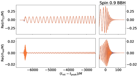
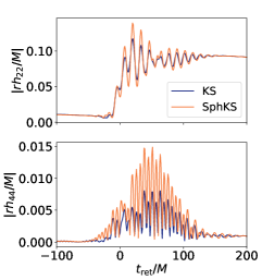
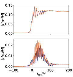
Figure 5: Strain $rh$ (extrapolated to $\mathscr{I}^{+}$) as a function of retarded time for the Lev-3 simulations. The top and bottom rows are for spin 0.9 and 0.99. The left column shows Re($rh_{22}$) and Re($rh_{44}$), while the right column shows $|rh_{22}|$ and $|rh_{44}|$. Waveforms in the left column are all time-shifted so that $|rh_{22}|$ (but not $|rh_{44}|$) reaches its maximum at time 0. They are also phase-shifted so that both $rh_{22}$ and $rh_{44}$ are real at time 0. Waveforms for KS and SphKS overlap well, except for the junk stage and tens of $M$ after merger in mode (4, 4). Waveforms in the right column are not time-shifted and only the junk parts are displayed. The amount of junk radiation for both gauges is comparable.

IV.2.1 Efficiency and constraint energy

The top left panel of Fig. 4 shows the CPU time ratio $T_{\text{SphKS}}/T_{\text{KS}}$ as a function of simulation time for the spin-0.9 BBH simulations, where $T_{\text{SphKS}}$ and $T_{\text{KS}}$ are the CPU times of SphKS and KS runs. A ratio smaller than 1 means SphKS is more efficient than KS. The smaller the ratio the more efficient the SphKS simulation is. Since all curves in the top left panel are below 1, the performance of SphKS runs is overall better. The ratio $T_{\text{SphKS}}/T_{\text{KS}}$ at the end of the simulation (after ringdown) is listed in Table 2, together with the CPU times. This CPU time ratio ranges from 0.79 to 0.91, which means a significant improvement for a BBH simulation by switching to the SphKS initial data.

The bottom left panel shows the constraint energy for both gauges. Solid lines stand for KS while dashed lines for SphKS. Curves of the same resolution (Lev) are plotted in the same color. We see that the constraint energy is similar for the same Lev between the SphKS and KS initial data. This is because AMR adjusts the target truncation error to control the constraint violations. What the top and bottom panels together show is that the SphKS initial data allows us to perform simulations with the same constraint violations at a reduced computational cost. Furthermore, we observe exponential convergence of the constraint energy between $t\sim 700M$ and merger. Before $t\sim 700M$, the curves in different Levs overlap, and their values are much greater than the later portion. This is because the AMR algorithm is disabled in the wave zone before $t\sim 700M$ to avoid using excessive computational resources to resolve the junk radiation.

IV.2.2 Waveforms

We extract the strain $h$ on multiple spherical surfaces of Euclidean radii $r$ and extrapolate $rh$ to $\mathscr{I}^{+}$ as a function of retarded time $t_{\text{ret}}$ [72, 73, 74, 75, 76]. Note that $rh$ is always center-of-mass-corrected in this paper. We show the $(l=2,m=2)$ and $(l=4,m=4)$ modes of $rh$, denoted as $rh_{22}$ and $rh_{44}$, in the first row of Fig. 5. Only the waveforms of the Lev-3 simulations are plotted. In each graph, the blue curve is data from the KS simulation and the orange curve from the SphKS simulation.

The top left diagram of Fig. 5 shows the real part of $rh_{22}$ and $rh_{44}$. For clearer comparison, these waveforms are both time-shifted and phase-shifted. Within the range of the retarded time $t_{\text{ret}}$, we choose the point $t_{\text{peak}}$ at which $|rh_{22}|$ reaches its maximum and shift the horizontal axis by $t_{\text{peak}}$. We then multiply each waveform by a phase such that the waveform is real and positive at $t_{\text{peak}}$. In other words, after time-shifting and phase-shifting, $|rh_{22}|$ is peaked (but not necessarily $|rh_{44}|$) at $t=t_{\text{peak}}$, and both $rh_{22}$ and $rh_{44}$ have zero phase at time $t_{\text{ret}}-t_{\text{peak}}=0$. This is similar to the procedure in Ref. [48]. The waveforms of the KS and SphKS simulations overlap very well after the junk radiation, $t_{\text{ret}}\gtrsim 700M$, except for some $\lesssim 0.001$ deviations after $t_{\text{ret}}-t_{\text{peak}}\sim 40M$ during the ringdown phase.

We quantify the similarity between two waveforms by the mismatch $\mathcal{M}$,

$$\mathcal{M}(h_{1},h_{2})=1-\max_{\delta\phi,\delta t}\left[\frac{|\langle h_{1}|h_{2,\delta\phi,\delta t}\rangle|}{\sqrt{\langle h_{1}|h_{1}\rangle\langle h_{2,\delta\phi,\delta t}|h_{2,\delta\phi,\delta t}\rangle}}\right],$$ (43)

where $h_{2,\delta\phi,\delta t}=e^{i\delta\phi}h_{2}(t+\delta t)$ and $h_{1},h_{2}$ are waveforms in a specific mode. $\delta\phi$ and $\delta t$ are parameters in phase- and time-shifting to maximize the overlap between two waveforms. The inner product $\langle\cdot|\cdot\rangle$ is defined as

$$\langle f|g\rangle=\int_{t_{i}}^{t_{f}}f(t)g^{*}(t)dt,$$ (44)

where * denotes complex conjugation. The mismatch is calculated for each mode ($h_{22}$ or $h_{44}$) over the time domain, unlike Ref. [25], which considers the strain $h$ before mode decomposition and calculates the inner product over the frequency domain. We choose $t_{i}$ to be $700M$ after the earliest time in KS Lev-3 waveform and $t_{f}=t_{\mathrm{peak}}+50M$. For both the $(2,2)$ and $(4,4)$ modes, the mismatch between KS Lev-2 and KS Lev-3 are at the same level as the mismatch between KS Lev-3 and SphKS Lev-3. Thus, the waveforms after junk radiation passes are in good agreement between KS and SphKS.

The high-frequency fluctuation within $t_{\text{ret}}\lesssim 700M$ is the transient gravitational perturbation called junk radiation. The origin of the junk radiation is the initial data not representing the true spacetime snapshot of a BBH system in quasi-equilibrium. The top right diagram of Fig. 5 shows $|rh_{22}|$ and $|rh_{44}|$ during the junk phase. This waveform is not time-shifted because we only care about the qualitative comparison of junk radiation between the two gauges. Note that the retarded time $t_{\text{ret}}$ can extend to negative values, and the waveform on this negative time axis corresponds to perturbations in the wave zone initial data. Both the KS and SphKS gauges produce roughly the same amount of junk radiation in the $(2,2)$ mode, while SphKS produces more than KS in the $(4,4)$ mode.

IV.3 Spin-0.99 binary-black-hole simulations using spherical Kerr-Schild initial data

We omit a discussion of the spin-0.95 BBH data and jump directly to the spin-0.99 BBH case because the efficiency and waveform comparisons are very similar.

IV.3.1 Efficiency, constraint energy and waveforms

The top right panel of Fig. 4 shows the CPU time ratio of the SphKS initial data to the KS initial data, while the bottom right panel of Fig. 4 shows the constraint energy at different resolutions for the two gauges. The curves and axes are labeled the same as for the spin-0.9 BBH case. Overall, the behavior of the CPU time ratio and constraint violations are similar to what we observed for the spin-0.9 simulations. Specifically, the constraint violations for the SphKS and KS initial data are very similar, while the simulations using SphKS initial data are cheaper than those using KS initial data. The Lev-3 spin-0.99 SphKS simulation is almost two times faster than the KS simulation.

The bottom row in Fig. 5 shows the waveforms of the spin-0.99 BBH simulations for the KS (blue) and SphKS (orange) initial data. The waveforms of the two gauges overlap well in both modes $(2,2)$ and $(4,4)$, except for some deviation at later times during ringdown. The mismatch [Eq. (43)] between KS Lev-3 and SphKS Lev-3 is also at the same order as between KS Lev-2 and Lev-3 for each mode. We note that both gauges have roughly the same amount (but not the exact same form) of junk radiation in both the $(2,2)$ and $(4,4)$ modes, in contrast with the spin-0.9 case, where the SphKS gauge $(4,4)$ mode had more junk radiation. The waveforms for both the SphKS and KS initial data being very similar and the SphKS initial data simulation being nearly twice as fast for higher resolutions demonstrate the advantage of using SphKS initial data for accurate and efficient high-spin BBH simulations.

IV.3.2 Apparent horizon analysis

SpEC decomposes the computational domain into multiple subdomains (Sec. II.3). There is an innermost spherical shell subdomain that encircles each BH and contains the BH’s apparent horizon (AH). The shape of the AH needs to be resolved, so we expect more spherical AHs to require lower resolutions. For concreteness, we will focus on the AHs of the Lev-3 spin-0.99 BBH simulations.

Figure 6 shows the AH profile of a progenitor-BH at two different times in the SphKS run. The left picture is at the beginning of evolution ($t=0M$) and clearly shows that the horizon is spherical in the SphKS gauge. At $t=0M$, the simulation starts to undergo a smooth transition from the quasi-equilibrium gauge to damped harmonic (DH) gauge, with the temporal width $w=50M$ (Sec. II.2). The right picture shows the AH at $t=50M$, at which point the AH is already non-spherical. In addition to the images of the AH, we record the angular resolution $L$ used to construct AHs by the AH finder [65], in the top panel of Fig. 7. The graph shows the angular resolution $L$ of Lev-3 runs in both gauges for $t<500M$. Because the AH in KS gauge starts as a distorted spheroid, the angular resolution $L$ in the KS simulation stays at $L=22$ immediately after the start and throughout the DH gauge transition. This suggests that the AH in the DH gauge is close to the spheroidal AH in the KS gauge. In the SphKS gauge, $L$ starts from a relatively low value (13) because of the spherical shape of the AH in the initial data and then climbs to a constant value throughout the DH gauge transition. This behavior of $L$ matches our expectation.

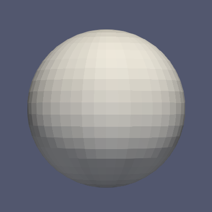
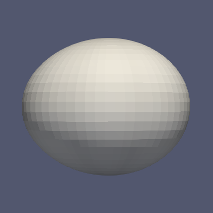
Figure 6: Apparent horizons of a progenitor-BH in the SphKS spin-0.99 Lev-3 BBH system, at $t=0M$ (left) and $t=50M$ (right). The apparent horizon is spherical at $t=0M$, which is a key feature of the SphKS gauge. The transition to damped harmonic gauge is mostly complete by $t=50M$, when we can see that the horizon is no longer spherical.

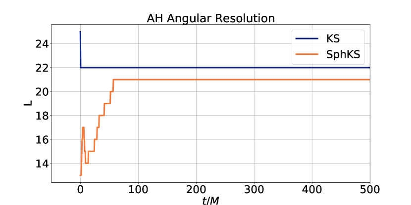
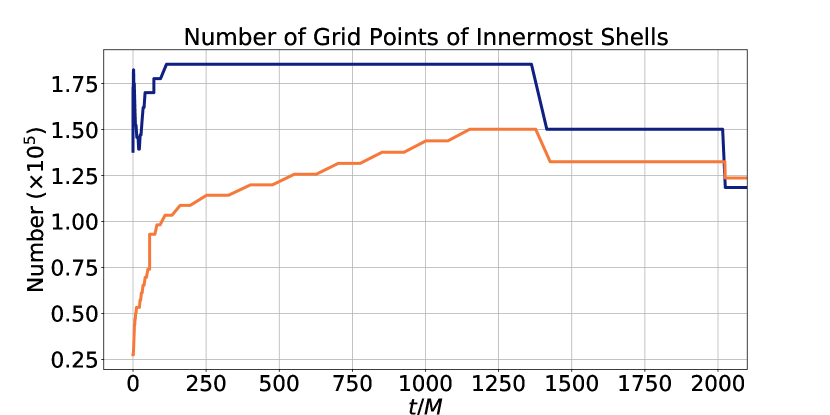
Figure 7: The top graph depicts the angular resolution $L$ used by the AH finder. $L$ in the KS run stays constant immediately after $t=0M$, suggesting that the AHs in the DH and KS gauges are similar. In the SphKS case, $L$ starts at a relatively low value and then increases to a constant during the DH gauge transition. The bottom graph records the total number of grid points in the innermost spheres surrounding the BHs.

Although the AHs quickly lose their spherical shape, we have found that the SphKS increases the speed of the simulation far beyond $t\sim 50M$ (see the top right panel of Fig. 4 and also the top left panel of Fig. 8). In the bottom panel of Fig. 7 we show the number of grid points in the innermost shell surrounding each BH. We see that even though the angular resolution used by the AH finder is nearly identical once the transition to DH gauge is complete, the number of points used near the BHs is significantly lower for the SphKS initial data all the way to $t\sim 2000M$.

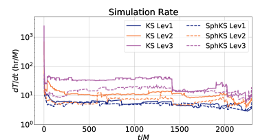
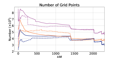
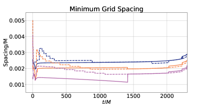
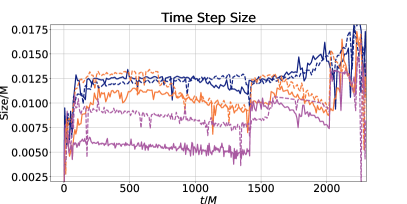
Figure 8: Four quantities related to the speed-up in the spin-0.99 BBH simulations. The top left graph shows the simulation rate $dT/dt$, and we see that the speed-up occurs throughout the evolution. The top right graph implies that the difference in the total number of grid points between two gauges cannot fully explain the speed-up. The bottom two graphs indicate that the narrower grid spacing in the KS simulations is a key factor making them slower than the SphKS simulations. The decreased grid spacing requires a smaller time step size and so the simulation progresses more slowly. Note that the abrupt change at $\sim 1400M$ in Lev-3 is shared among all four graphs and the bottom panel of Fig. 7 and is caused by an AMR decision.

IV.3.3 Speed-up analysis

Speeding-up the simulations significantly while keeping constraint violations and waveforms almost the same is encouraging. In this section we identify the contributions that lead to such a large speed-up. It is almost impossible to quantitatively decompose the speed-up into various algorithms’ contributions, but we may still obtain some qualitative insight from several relevant diagnostics of the evolution.

Figure 8 shows four such quantities. They are the simulation rate ($dT/dt$, i.e., the derivative of CPU time with respect to simulation time), total number of grid points, minimum grid spacing, and time step size. There are six curves in each graph, representing various Levs and gauges. Since most of the speed-up occurs before the merger ($\sim 2340M$), we restrict our plots to $0\leq t\leq 2300M$.

The earlier graph of CPU time ratio versus simulation time in Fig. 4 provides an overall comparison of computational cost. By contrast, an instantaneous comparison of efficiency between gauges can be quantified by the derivative $dT/dt$, as shown in the top left panel of Fig. 8. A slower simulation results in a higher curve in this graph, since more CPU time is required to compute a unit of simulation time. Given a fixed Lev, the curve for KS almost always lies above the one for SphKS, so a SphKS run is faster than a KS run not only collectively, but also at almost every moment. The difference in $dT/dt$ between gauges is larger as Lev increases, meaning that the SphKS gauge is especially useful if both high spin and high accuracy are desired, as seen previously in Fig. 4. We note that along the solid purple curve (KS Lev-3) in Fig. 8 the value of $dT/dt$ stays nearly constant after the beginning, but then plummets to the level of the dashed purple curve (SphKS Lev-3) at $\sim 1400M$. This drop is related to the AMR algorithm (Sec. II.3) rearranging the shells near the BHs. Attempts to replicate this domain configuration at earlier times led to unstable simulations. We will continue observing this behavior at $1400M$ throughout the next several graphs.

To better understand the source of the speed-up that the SphKS initial data provides, let us first look at the number of grid points used by the SphKS and KS simulations as a function of time. The top right panel of Fig. 8 shows the number of grid points as a function of time for both gauges and all three resolutions. While the Lev-1 and Lev-3 SphKS simulations have fewer grid points than KS, the trends of their curves do not match the $dT/dt$ curves. For example, the number of grid points for the Lev-3 simulations approach each other before $t\sim 250M$, while $dT/dt$ is still much smaller for the SphKS simulation. More surprisingly, the Lev-2 SphKS simulation uses more total grid points than the Lev-2 KS simulation but still has a smaller $dT/dt$. These differing trends between simulation rate and number of grid points suggests that there is another major contributing factor responsible for the observed speed-up.

Next we look at the Courant–Friedrichs–Lewy condition [77], by which the time step size is adjusted according to the spacing between grid points. If the spacing is narrower, then the time step size must be smaller, making the simulation slower. We plot the minimum grid spacing in the bottom left and the time step size in the bottom right panel of Fig. 8. We see that the minimum grid spacing for SphKS is larger than for KS in the first several hundred $M$, except for the region $t\lesssim 40M$. However, they both reach the same level later in the evolution for all Levs. The bottom right panel of Fig. 8 shows that the SphKS time step size is generally larger than the KS time step. Again, the difference is also more noticeable in the first several hundred $M$.

Focusing on the Lev-3 curves we see that SphKS has a larger minimum grid spacing, a larger time step size and faster simulation rate than KS in $40M<t<1400M$. We also check that the minimum grid spacing is always located in the innermost shells near BHs in this time range for both KS and SphKS simulations. Around $1400M$ in the KS simulation AMR changes the grid, resulting in fewer grid points in the innermost shells (see Fig. 7) and a minimum grid spacing, and a time step comparable to the SphKS case. At this point, the SphKS and KS simulations also have approximately the same $dT/dt$. This leads us to conclude that the more sparse distribution of grid points near the BHs in a simulation with SphKS initial data is the major contributing factor to the speed-up.

IV.4 Binary-black-hole simulations using wide Kerr-Schild initial data

We evolve a 25-orbit, non-precessing, non-eccentric, equal-mass, spin-0.9 BBH system using the wide Kerr-Schild (WKS) gauge (Sec. III.2) with $b=0.95$ and $b=0.9$ (recall that $b=1$ corresponds to the SphKS gauge). The parameters of initial setup are listed in Table 3. Their values are close to the previous spin-0.9 SphKS BBH run, so we compare these three simulations together.

Table 3: Parameters of three BBH simulations using WKS initial data with $b\in\{1,0.95,0.9\}$. Note that WKS of $b=1$ is equivalent to SphKS. In all three simulations, the mass ratio is 1, $\chi_{A,B}=(0,0,0.9)$, and the number of orbits is about 25. See Table 1 for definitions of parameters.

Initial gauge	$D_{0}$ $[M]$	$\Omega_{0}$	$\dot{a}_{0}$	$e$
SphKS	15.450	0.0142	4.53$\times 10^{-4}$	$\sim 0.0005$
WKS b0.95	15.452	0.0142	4.56$\times 10^{-4}$	$\sim 0.0003$
WKS b0.9	15.455	0.0142	4.51$\times 10^{-4}$	$\sim 0.0003$

We find that the WKS simulations share most of the properties of the SphKS simulations. Namely, there is no consistent improvement in either CPU efficiency or constraint energy by switching from SphKS to WKS. Both the strain modes Re$(rh_{22})$ and Re$(rh_{44})$ from different gauges overlap well. However, the amount of junk radiation significantly increases when $b\neq 1$. We find that the junk is approximately doubled when $b=0.9$ compared to $b=1$. Therefore, we do not recommend the use of WKS for evolutions of high-spin BBHs.

IV.5 Binary-black-hole simulations with delayed evolution gauge transition

In this section, we simulate BBH systems in SphKS where we delay the transition from the initial spherical gauge to damped harmonic (DH) gauge with the hope that this further improves efficiency. We choose $t_{0}=4000M$ and $w\in\{50M,100M,400M\}$ [see Eq. (22) for the definitions of $t_{0}$ and $w$]. All of these cases share the same initial parameters with the non-delayed-transition SphKS spin-0.9 run in Table 1. All runs have negligible eccentricity ($e<0.0007$), and we only focus on the highest resolution, Lev-3.

IV.5.1 Efficiency and constraint energy

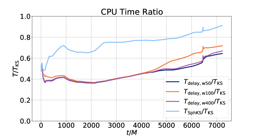
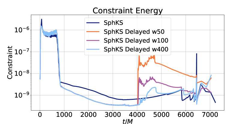
Figure 9: CPU time ratio $T/T_{\text{KS}}$ (top panel) and constraint energy (bottom panel) of the spin-0.9 Lev-3 BBH in SphKS and delayed SphKS. The speed-up by delaying the evolution gauge is manifest, by a factor of 1.3 compared to SphKS and 1.5 compared to KS. We see that the speed-up of the delayed runs is mostly independent of the transition width. However, a large increase in the constraint violations is observed at the moment the gauge transition is started ($t=4000M$). Constraint violations in the delayed gauge can reach several orders of magnitude higher than the non-delayed one, immediately after the transition time $t=4000M$.

We plot the CPU time ratio $T/T_{\text{KS}}$ in the top panel of Fig. 9. $T_{\text{KS}}$, $T_{\text{SphKS}}$, and $T_{\text{delay}}$ are the CPU times of simulations with the KS initial data, the SphKS initial data without delay, and the SphKS initial data with delayed transition of various widths $w$. A clear improvement is seen in all delayed simulations, with the average reduction in final runtime being $\sim 25\%$ compared to SphKS and $\sim 32\%$ compared to KS.

The temporal part of the DH gauge transition function has a discontinuous fourth derivative at $t_{0}$ [Eq. (22)], which the high-order methods employed by SpEC may be sensitive to. The fourth derivative is proportional to $1/w^{4}$, so a narrower width introduces a larger discontinuity in the derivative, which can lead to larger numerical errors. This feature shows up in the constraint energy plot (the bottom panel of Fig. 9). All runs have the same order of constraint violations before 4000$M$, but later the curves of delayed runs abruptly jump up by several orders of magnitude at 4000$M$. The jump in the constraint energy is larger as the temporal width gets narrower since the derivative is larger and the gauge transition is steeper. This graph also suggests that only a width of at least 400$M$ would be acceptable for production BBH simulations.

IV.5.2 Waveforms

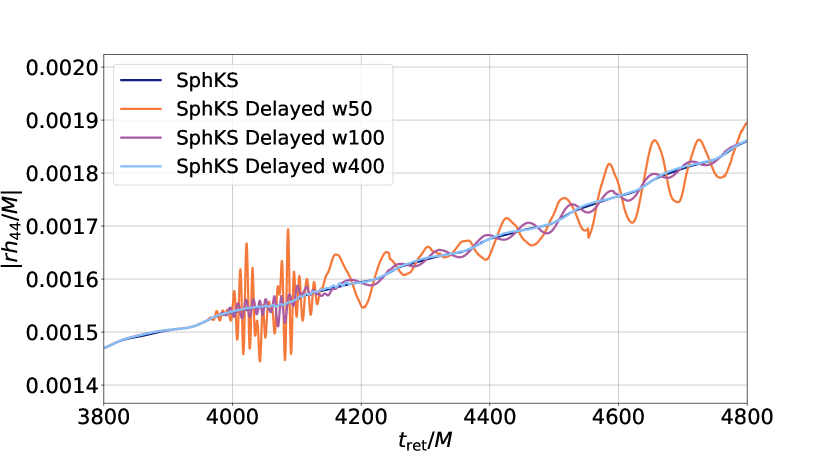
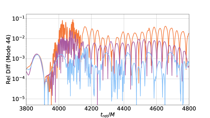
Figure 10: A comparison of the strain $rh$ between SphKS and delayed SphKS for the spin-0.9 Lev-3 BBH simulations. The top panel shows $|rh_{44}|$ in $3800M<t_{\text{ret}}<4800M$. We see the unexpected fluctuation in the delayed transition curves for all three temporal widths. To better see how the oscillations change with increasing width, the bottom panel depicts the relative difference in $|rh_{44}|$ of the delayed SphKS compared to the SphKS simulations. The fluctuation is greater as the temporal width $w$ becomes narrower.

The large jump in the constraint violations at $t=4000M$ may result in unphysical effects in the waveforms. We plot $|rh_{44}|$ in the top panel of Fig. 10 on the interval $3800M<t_{\text{ret}}<4800M$. We see that large oscillations appear at $t=4000M$ in the delayed transition waveforms that are absent in the non-delayed run. The amplitude of the oscillations decreases with increasing width. This is not surprising considering that the discontinuity in the fourth derivative of the roll-off function decreases as $1/w^{4}$. Note that the waveforms in different gauges overlap before the transition, suggesting that the oscillations are an artifact of the non-smooth gauge transition.

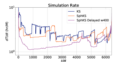
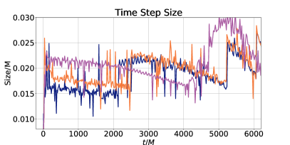
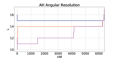
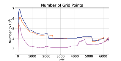
Figure 11: Four quantities for the speed-up analysis of delaying the DH gauge transition in the spin-0.9 Lev-3 BBH runs. The top left panel shows that a simulation in delayed SphKS is faster at almost every moment before 4000$M$. In the top right panel, we see the same level of time step sizes between non-delayed and delayed gauges, so time step is not a contributing factor of the speed-up. The bottom left graph confirms that the AH stays close to spherical before the onset of the gauge transition. From the bottom right graph, we conclude that the significantly smaller amount of grid points is responsible for the speed-up from delaying the gauge transition.

To better see how the fluctuations depend on the transition width $w$, we calculate the relative difference in $|rh_{44}|$ of the three delayed runs compared to the non-delayed one, in the bottom panel of Fig. 10. The difference is in general smaller as the transition width increases, which is reasonable since a narrower transition induces a larger discontinuity in the fourth derivatives. For example, the width-50$M$ curve has relative differences at the order of $10^{-1}$, while the width-400$M$ differences are $10^{-3}$.

To better understand how smoothness in a delayed gauge transition function affects a waveform, we simulate the same BBH system as above with SphKS initial data but with a different gauge transition temporal function. Instead of Eq. (22), we use

$$F(t)=\exp\left[-\left(\frac{t}{3500M}\right)^{10}\right],\quad t\geq 0.$$ (45)

This temporal function is smooth after the start of a simulation and delays the DH gauge until $t\sim 2600M$ [when $F(t)=0.95$]. The waveforms $rh_{22}$ and $rh_{44}$ have relative difference (compared to the non-delayed SphKS simulation) at the same order as the $t_{0}=4000M,w=400M$ SphKS simulation. We find that the high-frequency noise in the waveforms is greatly reduced, but not completely eliminated. Thus, the smoothness in the temporal transition of the evolution gauge is a factor causing the high-frequency fluctuation, but not the main factor.

Given the growth in constraint violations and the appearance of fluctuations in the waveforms, we do not recommend delaying the gauge transition despite the significant speed-up of the simulations.

IV.5.3 Speed-up analysis

In this section, we examine the mechanism of the speed-up from delaying the DH gauge transition.We consider three spin-0.9 Lev-3 simulations: KS initial data, SphKS initial data without delay, and SphKS initial data with the delayed gauge transition of width $w=400M$. Figure 11 shows the simulation rate $dT/dt$, time step size, angular resolution $L$ used by the AH finder, and total number of grid points in these three simulations. The blue curves represent the simulation with the KS initial data, the orange curves are for the non-delayed SphKS simulation, and the purple ones for the $w=400M$ delayed transition SphKS simulation.

The graph of simulation rate (the top left panel of Fig. 11) indicates that the delayed SphKS simulation is more efficient than the other two gauges at almost any time, especially before the transition time $t=4000M$. The top right panel of Fig. 11 shows that the time step sizes for the different gauges are nearly equal, so the time step has no contribution to the speed-up. In the bottom left panel of Fig. 11, we see that the angular resolution $L$ in the delayed SphKS simulation is initially relatively low but then climbs to the level of the other two gauges near $t=4000M$. This is expected because the AH is spherical in the SphKS coordinates but highly non-spherical in the DH gauge, and delaying the transition keeps the AH in a nearly spherical shape until $t=t_{0}=4000M$. The bottom right graph of Fig. 11 shows that the total number of grid points in the delayed SphKS run is considerably smaller than the other two gauges, especially before $t=4000M$. Note that the number of grid points for delayed SphKS is 19%–32% smaller than the other two gauges when $1000M<t<4000M$, which is comparable to the overall efficiency improvement ($1-T_{\text{delay,w400}}/T_{\text{SphKS}}=26\%$). Thus, in a SphKS simulation, delaying the DH gauge transition accelerates the computation by substantially reducing the number of grid points.

V Conclusion

In this paper, we develop new gauge conditions for BHs with the goal of reducing the computational cost of high-spin BBH simulations. We present several different attempts, among which the most promising is the use of spherical Kerr-Schild, where the horizons of a rotating BH are spherical. For single BH evolutions using spherical Kerr-Schild, we find a factor of 10 reduction in the metric error and 1000 in the constraint energy, as compared to Kerr-Schild with the same resolution. For BBH evolutions, we see efficiency improvement with equal accuracy. In general, we find that the speed-up is greater for simulations with stricter truncation error tolerances and higher spin. Specifically, we observe an impressive factor of 2 reduction in CPU time for the spin-0.99 Lev-3 (standard resolution of SXS BBH simulations) case. This new gauge condition will also reduce the computational cost of extending BBH simulations to higher spins (e.g., $\chi=0.999$), allowing waveform catalogs and models (such as surrogates [33, 34, 35, 36]) tuned to numerical relativity to cover a larger and denser portion of the mass-spin parameter space with significantly reduced cost.

While the main focus of this paper has been improvements by changing the initial data, we also performed some experiments where we delay the transition from the initial data gauge to the damped harmonic gauge used in the evolution. The goal is to keep the horizons spherical for longer so that this further reduces the computational cost of the simulations. In Sec. IV.5, we find that imposing a spherical gauge condition during the evolution will produce an additional speed-up by a factor of 1.3. However, one must be careful not to introduce artifacts into the waveforms when delaying the gauge transition.

Inspired by the benefit of delaying the evolution gauge, we expect a dynamical spherical gauge condition to be very useful for simulating high-spin BBHs. As future work, one can develop a spherical version of damped harmonic gauge, where the horizons of BHs can remain (nearly) spherical during the whole evolution. As far as the initial data gauge is concerned, one may consider blending the spherical Kerr-Schild and harmonic-Kerr spatially, or even developing a spherical version of harmonic-Kerr with the hope to reduce both the computational cost and junk radiation. Nonetheless, solely changing the initial data as described in this paper is certainly worthwhile.

Appendix A $\gamma_{0},\gamma_{1},\gamma_{2}$, and $\gamma_{3}$ used in simulations

SpEC evolves the spacetime of BHs in the first order GH formalism [44], which is given by Eqs. (16$-$18). We consider four constraint damping parameters in this formalism for this paper, namely $\gamma_{0},\gamma_{1},\gamma_{2}$, and $\gamma_{3}$. These parameters have been used to simulate BHs in previous papers. The quantities $\gamma_{0}$, $\gamma_{1}$, and $\gamma_{2}$ are the same as those in Refs. [44, 68]. These three parameters are set to nonzero values by default in a SpEC BBH simulation. $\gamma_{3}$ in this paper is different from the $\gamma_{3}$ used in Ref. [44]. Instead, our $\gamma_{3}$ is the same as the parameter $\rho$ used in Ref. [58]. The authors of Ref. [58] set this parameter to 0 by default, while we explore the possibility of a nonzero $\gamma_{3}$ for single BH simulations in this paper.

We here provide the expressions of $\gamma_{0},\gamma_{1},\gamma_{2}$, and $\gamma_{3}$ used for simulations in this paper. Specifically, for single BH simulations, we choose

$$\gamma_{0}M=\gamma_{2}M =2\exp\left[-\left(\frac{r_{O}}{7M}\right)^{2}\right]+0.001,$$ (46)

$$\gamma_{1} =-1,$$ (47)

$$\gamma_{3} =2,$$ (48)

where $M$ is the total ADM mass of the system as usual. $\gamma_{0}$ and $\gamma_{2}$ are spatially varying and depend on $r_{O}$, the Euclidean distance from the origin. We choose the origin at the geometric center of a single BH. The choice $\gamma_{1}=-1$ is adopted in the simulations of Ref. [44] as well, which makes the GH system Eqs. (16$-$18) linearly degenerate. Note that $\gamma_{0}$, $\gamma_{2}$ have dimension $M^{-1}$ while $\gamma_{1}$, $\gamma_{3}$ are dimensionless.

The expressions of the parameters for BBHs are more complicated than for single BHs. In the ringdown phase, we use

$$\gamma_{0}M=\gamma_{2}M =0.001+7\exp\left[-\left(\frac{r_{O}}{2.5M}\right)^{2}\right]$$

$$\quad+0.1\exp\left[-\left(\frac{r_{O}}{100M}\right)^{2}\right],$$ (49)

$$\gamma_{1} =-1,$$ (50)

$$\gamma_{3} =0.$$ (51)

In the inspiral phase, we use

$$\gamma_{0}M=\gamma_{2}M =0.001+0.075\exp\left[-\left(\frac{r_{O}a_{\mathrm{scale}}}{2.5D_{0}}\right)^{2}\right]$$

$$\quad+\frac{4M}{M_{A}}\exp\left[-\left(\frac{r_{A}a_{\mathrm{scale}}}{7M_{A}}\right)^{2}\right]$$

$$\quad+\frac{4M}{M_{B}}\exp\left[-\left(\frac{r_{B}a_{\mathrm{scale}}}{7M_{B}}\right)^{2}\right],$$ (52)

$$\gamma_{1} =0.999\left\{\exp\left[-\left(\frac{r_{O}}{10D_{0}}\right)^{2}\right]-1\right\},$$ (53)

$$\gamma_{3} =0,$$ (54)

where $M_{A},M_{B}$ are the initial Christoudoulou masses [78] of BH $A,B$, and $r_{A},r_{B}$ are the Euclidean distances from BH $A,B$. $D_{0}$ is the initial separation between the two BHs, used in Tables I and III. $a_{\mathrm{scale}}$ is equivalent to the (dimensionless) expansion factor $a$ used in Refs. [64, 65]. $a_{\mathrm{scale}}$ is tuned by the control system in SpEC [65], so it is time-dependent. The three distance variables $r_{A}$, $r_{B}$, and $r_{O}$ are measured in the distorted frame of a BBH simulation. The distorted frame is an intermediate frame between the grid frame and the inertial frame, and we point interested readers to Ref. [65] for details on the relation among these frames. Note that we do not specify the measurement frame of $r_{O}$ for a single BH simulation, because the grid, the distorted and the inertial frames are identical for single BHs in this paper.

References

- Abbott et al. [2016a] B. P. Abbott et al. (LIGO Scientific, Virgo), Observation of Gravitational Waves from a Binary Black Hole Merger, Phys. Rev. Lett. 116, 061102 (2016a), arXiv:1602.03837 [gr-qc] .
- Abbott et al. [2016b] B. P. Abbott et al. (LIGO Scientific, Virgo), GW150914: First results from the search for binary black hole coalescence with Advanced LIGO, Phys. Rev. D93, 122003 (2016b), arXiv:1602.03839 [gr-qc] .
- Abbott et al. [2016c] B. P. Abbott et al. (LIGO Scientific, Virgo), GW150914: The Advanced LIGO Detectors in the Era of First Discoveries, Phys. Rev. Lett. 116, 131103 (2016c), arXiv:1602.03838 [gr-qc] .
- Abbott et al. [2016d] B. P. Abbott et al. (LIGO Scientific, Virgo), Properties of the Binary Black Hole Merger GW150914, Phys. Rev. Lett. 116, 241102 (2016d), arXiv:1602.03840 [gr-qc] .
- Abbott et al. [2019] B. P. Abbott et al. (LIGO Scientific, Virgo), GWTC-1: A Gravitational-Wave Transient Catalog of Compact Binary Mergers Observed by LIGO and Virgo during the First and Second Observing Runs, Phys. Rev. X9, 031040 (2019), arXiv:1811.12907 [astro-ph.HE] .
- Abbott et al. [2021] R. Abbott et al. (LIGO Scientific, Virgo), GWTC-2: Compact Binary Coalescences Observed by LIGO and Virgo During the First Half of the Third Observing Run, Phys. Rev. X11, 021053 (2021), arXiv:2010.14527 [gr-qc] .
- Abbott et al. [2020a] R. Abbott et al. (LIGO Scientific, Virgo), GW190521: A Binary Black Hole Merger with a Total Mass of , Phys. Rev. Lett. 125, 101102 (2020a), arXiv:2009.01075 [gr-qc] .
- Blanchet [2014] L. Blanchet, Gravitational Radiation from Post-Newtonian Sources and Inspiralling Compact Binaries, Living Rev. Rel. 17, 2 (2014), arXiv:1310.1528 [gr-qc] .
- Abbott et al. [2020b] R. Abbott et al. (LIGO Scientific, Virgo), Properties and Astrophysical Implications of the 150 M⊙ Binary Black Hole Merger GW190521, Astrophys. J. Lett. 900, L13 (2020b), arXiv:2009.01190 [astro-ph.HE] .
- Berti et al. [2015] E. Berti et al., Testing General Relativity with Present and Future Astrophysical Observations, Class. Quant. Grav. 32, 243001 (2015), arXiv:1501.07274 [gr-qc] .
- Abbott et al. [2016e] B. P. Abbott et al. (LIGO Scientific, Virgo), Tests of general relativity with GW150914, Phys. Rev. Lett. 116, 221101 (2016e), [Erratum: Phys. Rev. Lett.121,no.12,129902(2018)], arXiv:1602.03841 [gr-qc] .
- Berti et al. [2018a] E. Berti, K. Yagi, H. Yang, and N. Yunes, Extreme Gravity Tests with Gravitational Waves from Compact Binary Coalescences: (II) Ringdown, Gen. Rel. Grav. 50, 49 (2018a), arXiv:1801.03587 [gr-qc] .
- Berti et al. [2018b] E. Berti, K. Yagi, and N. Yunes, Extreme Gravity Tests with Gravitational Waves from Compact Binary Coalescences: (I) Inspiral-Merger, Gen. Rel. Grav. 50, 46 (2018b), arXiv:1801.03208 [gr-qc] .
- Pretorius [2005a] F. Pretorius, Evolution of binary black hole spacetimes, Phys. Rev. Lett. 95, 121101 (2005a), arXiv:gr-qc/0507014 [gr-qc] .
- Baker et al. [2006] J. G. Baker, J. Centrella, D.-I. Choi, M. Koppitz, and J. van Meter, Gravitational wave extraction from an inspiraling configuration of merging black holes, Phys. Rev. Lett. 96, 111102 (2006), arXiv:gr-qc/0511103 [gr-qc] .
- Campanelli et al. [2006] M. Campanelli, C. O. Lousto, P. Marronetti, and Y. Zlochower, Accurate evolutions of orbiting black-hole binaries without excision, Phys. Rev. Lett. 96, 111101 (2006), arXiv:gr-qc/0511048 [gr-qc] .
- Aylott et al. [2009] B. Aylott et al., Status of NINJA: The Numerical INJection Analysis project, Class. Quant. Grav. 26, 114008 (2009), arXiv:0905.4227 [gr-qc] .
- Ajith et al. [2012] P. Ajith et al., The NINJA-2 catalog of hybrid post-Newtonian/numerical-relativity waveforms for non-precessing black-hole binaries, Class. Quant. Grav. 29, 124001 (2012), [Erratum: Class. Quant. Grav. 30, 199401 (2013)], arXiv:1201.5319 [gr-qc] .
- Mroue et al. [2013] A. H. Mroue, M. A. Scheel, B. Szilágyi, H. P. Pfeiffer, M. Boyle, and D. A. Hemberger, Catalog of 174 Binary Black Hole Simulations for Gravitational Wave Astronomy, Phys. Rev. Lett. 111, 241104 (2013), arXiv:1304.6077 [gr-qc] .
- Hinder et al. [2014] I. Hinder et al., Error-analysis and comparison to analytical models of numerical waveforms produced by the NRAR Collaboration, Class. Quant. Grav. 31, 025012 (2014), arXiv:1307.5307 [gr-qc] .
- Jani et al. [2016] K. Jani, J. Healy, J. A. Clark, L. London, P. Laguna, and D. Shoemaker, Georgia Tech Catalog of Gravitational Waveforms, Class. Quant. Grav. 33, 204001 (2016), arXiv:1605.03204 [gr-qc] .
- Healy et al. [2017] J. Healy, C. O. Lousto, Y. Zlochower, and M. Campanelli, The RIT binary black hole simulations catalog, Class. Quant. Grav. 34, 224001 (2017), arXiv:1703.03423 [gr-qc] .
- Healy et al. [2019] J. Healy, C. O. Lousto, J. Lange, R. O’Shaughnessy, Y. Zlochower, and M. Campanelli, Second RIT binary black hole simulations catalog and its application to gravitational waves parameter estimation, Phys. Rev. D100, 024021 (2019), arXiv:1901.02553 [gr-qc] .
- Huerta et al. [2019] E. A. Huerta et al., Physics of eccentric binary black hole mergers: A numerical relativity perspective, Phys. Rev. D100, 064003 (2019), arXiv:1901.07038 [gr-qc] .
- Boyle et al. [2019] M. Boyle et al., The SXS Collaboration catalog of binary black hole simulations, Class. Quant. Grav. 36, 195006 (2019), arXiv:1904.04831 [gr-qc] .
- Gou et al. [2011] L. Gou, J. E. McClintock, M. J. Reid, J. A. Orosz, J. F. Steiner, R. Narayan, J. Xiang, R. A. Remillard, K. A. Arnaud, and S. W. Davis, The Extreme Spin of the Black Hole in Cygnus X-1, Astrophys. J. 742, 85 (2011), arXiv:1106.3690 [astro-ph.HE] .
- Fabian et al. [2012] A. C. Fabian et al., On the determination of the spin of the black hole in Cyg X-1 from X-ray reflection spectra, Mon. Not. Roy. Astron. Soc. 424, 217 (2012), arXiv:1204.5854 [astro-ph.HE] .
- Gou et al. [2014] L. Gou, J. E. McClintock, R. A. Remillard, J. F. Steiner, M. J. Reid, J. A. Orosz, R. Narayan, M. Hanke, and J. García, Confirmation Via the Continuum-Fitting Method that the Spin of the Black Hole in Cygnus X-1 is Extreme, Astrophys. J. 790, 29 (2014), arXiv:1308.4760 [astro-ph.HE] .
- Miller et al. [2009] J. M. Miller, C. S. Reynolds, A. C. Fabian, G. Miniutti, and L. C. Gallo, Stellar-mass Black Hole Spin Constraints from Disk Reflection and Continuum Modeling, Astrophys. J. 697, 900 (2009), arXiv:0902.2840 [astro-ph.HE] .
- McClintock et al. [2006] J. E. McClintock, R. Shafee, R. Narayan, R. A. Remillard, S. W. Davis, and L.-X. Li, The Spin of the Near-Extreme Kerr Black Hole GRS 1915+105, Astrophys. J. 652, 518 (2006), arXiv:astro-ph/0606076 [astro-ph] .
- Healy and Lousto [2018] J. Healy and C. O. Lousto, Hangup effect in unequal mass binary black hole mergers and further studies of their gravitational radiation and remnant properties, Phys. Rev. D97, 084002 (2018), arXiv:1801.08162 [gr-qc] .
- Lousto and Healy [2015] C. O. Lousto and J. Healy, Flip-flopping binary black holes, Phys. Rev. Lett. 114, 141101 (2015), arXiv:1410.3830 [gr-qc] .
- Blackman et al. [2015] J. Blackman, S. E. Field, C. R. Galley, B. Szilagyi, M. A. Scheel, M. Tiglio, and D. A. Hemberger, Fast and Accurate Prediction of Numerical Relativity Waveforms from Binary Black Hole Coalescences Using Surrogate Models, Phys. Rev. Lett. 115, 121102 (2015), arXiv:1502.07758 [gr-qc] .
- Blackman et al. [2017a] J. Blackman, S. E. Field, M. A. Scheel, C. R. Galley, D. A. Hemberger, P. Schmidt, and R. Smith, A Surrogate Model of Gravitational Waveforms from Numerical Relativity Simulations of Precessing Binary Black Hole Mergers, Phys. Rev. D95, 104023 (2017a), arXiv:1701.00550 [gr-qc] .
- Blackman et al. [2017b] J. Blackman, S. E. Field, M. A. Scheel, C. R. Galley, C. D. Ott, M. Boyle, L. E. Kidder, H. P. Pfeiffer, and B. Szilagyi, Numerical relativity waveform surrogate model for generically precessing binary black hole mergers, Phys. Rev. D96, 024058 (2017b), arXiv:1705.07089 [gr-qc] .
- Varma et al. [2019a] V. Varma, S. E. Field, M. A. Scheel, J. Blackman, L. E. Kidder, and H. P. Pfeiffer, Surrogate model of hybridized numerical relativity binary black hole waveforms, Phys. Rev. D99, 064045 (2019a), arXiv:1812.07865 [gr-qc] .
- Buonanno and Damour [1999] A. Buonanno and T. Damour, Effective one-body approach to general relativistic two-body dynamics, Phys. Rev. D59, 084006 (1999), arXiv:gr-qc/9811091 [gr-qc] .
- Damour and Nagar [2008] T. Damour and A. Nagar, Comparing Effective-One-Body gravitational waveforms to accurate numerical data, Phys. Rev. D77, 024043 (2008), arXiv:0711.2628 [gr-qc] .
- Pan et al. [2014] Y. Pan, A. Buonanno, A. Taracchini, L. E. Kidder, A. H. Mroue, H. P. Pfeiffer, M. A. Scheel, and B. Szilagyi, Inspiral-merger-ringdown waveforms of spinning, precessing black-hole binaries in the effective-one-body formalism, Phys. Rev. D89, 084006 (2014), arXiv:1307.6232 [gr-qc] .
- Bohe et al. [2017] A. Bohe, L. Shao, A. Taracchini, A. Buonanno, S. Babak, I. W. Harry, et al., Improved effective-one-body model of spinning, nonprecessing binary black holes for the era of gravitational-wave astrophysics with advanced detectors, Phys. Rev. D95, 044028 (2017), arXiv:1611.03703 [gr-qc] .
- Varma et al. [2019b] V. Varma, S. E. Field, M. A. Scheel, J. Blackman, D. Gerosa, L. C. Stein, L. E. Kidder, and H. P. Pfeiffer, Surrogate models for precessing binary black hole simulations with unequal masses, Phys. Rev. Research. 1, 033015 (2019b), arXiv:1905.09300 [gr-qc] .
- Taracchini et al. [2014] A. Taracchini et al., Effective-one-body model for black-hole binaries with generic mass ratios and spins, Phys. Rev. D89, 061502(R) (2014), arXiv:1311.2544 [gr-qc] .
- [43] http://www.black-holes.org/SpEC.html.
- Lindblom et al. [2006] L. Lindblom, M. A. Scheel, L. E. Kidder, R. Owen, and O. Rinne, A New generalized harmonic evolution system, Class. Quant. Grav. 23, S447 (2006), arXiv:gr-qc/0512093 [gr-qc] .
- York [1999] J. W. York, Jr., Conformal ’thin sandwich’ data for the initial-value problem, Phys. Rev. Lett. 82, 1350 (1999), arXiv:gr-qc/9810051 [gr-qc] .
- Pfeiffer and York [2003] H. P. Pfeiffer and J. W. York, Jr., Extrinsic curvature and the Einstein constraints, Phys. Rev. D67, 044022 (2003), arXiv:gr-qc/0207095 [gr-qc] .
- Lovelace et al. [2008] G. Lovelace, R. Owen, H. P. Pfeiffer, and T. Chu, Binary-black-hole initial data with nearly-extremal spins, Phys. Rev. D78, 084017 (2008), arXiv:0805.4192 [gr-qc] .
- Varma et al. [2018] V. Varma, M. A. Scheel, and H. P. Pfeiffer, Comparison of binary black hole initial data sets, Phys. Rev. D98, 104011 (2018), arXiv:1808.08228 [gr-qc] .
- Ma et al. [2021] S. Ma, M. Giesler, M. A. Scheel, and V. Varma, Extending superposed harmonic initial data to higher spin, Phys. Rev. D103, 084029 (2021), arXiv:2102.06618 [gr-qc] .
- Baumgarte and Shapiro [2010] T. W. Baumgarte and S. L. Shapiro, Numerical Relativity: Solving Einstein’s Equations on the Computer (Cambridge University Press, 2010).
- Pfeiffer et al. [2003] H. P. Pfeiffer, L. E. Kidder, M. A. Scheel, and S. A. Teukolsky, A Multidomain spectral method for solving elliptic equations, Comput. Phys. Commun. 152, 253 (2003), arXiv:gr-qc/0202096 [gr-qc] .
- Friedrich [1985] H. Friedrich, On the hyperbolicity of Einstein’s and other gauge field equations, Commun. Math. Phys. 100, 525–543 (1985).
- Garfinkle [2002] D. Garfinkle, Harmonic coordinate method for simulating generic singularities, Phys. Rev. D65, 044029 (2002), arXiv:gr-qc/0110013 [gr-qc] .
- Pretorius [2005b] F. Pretorius, Numerical relativity using a generalized harmonic decomposition, Class. Quant. Grav. 22, 425 (2005b), arXiv:gr-qc/0407110 [gr-qc] .
- Scheel et al. [2004] M. A. Scheel, A. L. Erickcek, L. M. Burko, L. E. Kidder, H. P. Pfeiffer, and S. A. Teukolsky, 3-D simulations of linearized scalar fields in Kerr space-time, Phys. Rev. D69, 104006 (2004), arXiv:gr-qc/0305027 [gr-qc] .
- Holst et al. [2004] M. Holst, L. Lindblom, R. Owen, H. P. Pfeiffer, M. A. Scheel, and L. E. Kidder, Optimal constraint projection for hyperbolic evolution systems, Phys. Rev. D70, 084017 (2004), arXiv:gr-qc/0407011 [gr-qc] .
- Lindblom et al. [2004] L. Lindblom, M. A. Scheel, L. E. Kidder, H. P. Pfeiffer, D. Shoemaker, and S. A. Teukolsky, Controlling the growth of constraints in hyperbolic evolution systems, Phys. Rev. D69, 124025 (2004), arXiv:gr-qc/0402027 [gr-qc] .
- Gundlach et al. [2005] C. Gundlach, J. M. Martin-Garcia, G. Calabrese, and I. Hinder, Constraint damping in the Z4 formulation and harmonic gauge, Class. Quant. Grav. 22, 3767 (2005), arXiv:gr-qc/0504114 [gr-qc] .
- Renn and Sauer [1999] J. Renn and T. Sauer, Heuristics and Mathematical Representation in Einstein’s Search for a Gravitational Field Equation, in The Expanding Worlds of General Relativity, edited by H. Goenner, J. Renn, J. Ritter, and T. Sauer (Birkhäuser, Basel, 1999) p. 87.
- de Donder [1922] T. de Donder, La gravifique einsteinienne, Annales de l’Observatoire Royal de Belgique 1, 73 (1922).
- Fock [1959] V. Fock, Theory of Space: Time and Gravitation (Pergamon Press, 1959).
- Fischer and Marsden [1972] A. E. Fischer and J. E. Marsden, The Einstein evolution equations as a first-order quasi-linear symmetric hyperbolic system, Commun. Math. Phys. 28, 1 (1972).
- Szilagyi et al. [2009] B. Szilagyi, L. Lindblom, and M. A. Scheel, Simulations of Binary Black Hole Mergers Using Spectral Methods, Phys. Rev. D80, 124010 (2009), arXiv:0909.3557 [gr-qc] .
- Scheel et al. [2006] M. A. Scheel, H. P. Pfeiffer, L. Lindblom, L. E. Kidder, O. Rinne, and S. A. Teukolsky, Solving Einstein’s equations with dual coordinate frames, Phys. Rev. D74, 104006 (2006), arXiv:gr-qc/0607056 [gr-qc] .
- Hemberger et al. [2013] D. A. Hemberger, M. A. Scheel, L. E. Kidder, B. Szilagyi, G. Lovelace, N. W. Taylor, and S. A. Teukolsky, Dynamical Excision Boundaries in Spectral Evolutions of Binary Black Hole Spacetimes, Class. Quant. Grav. 30, 115001 (2013), arXiv:1211.6079 [gr-qc] .
- Buchman et al. [2012] L. T. Buchman, H. P. Pfeiffer, M. A. Scheel, and B. Szilagyi, Simulations of non-equal mass black hole binaries with spectral methods, Phys. Rev. D86, 084033 (2012), arXiv:1206.3015 [gr-qc] .
- Lovelace et al. [2011] G. Lovelace, M. A. Scheel, and B. Szilagyi, Simulating merging binary black holes with nearly extremal spins, Phys. Rev. D83, 024010 (2011), arXiv:1010.2777 [gr-qc] .
- Szilagyi [2014] B. Szilagyi, Key Elements of Robustness in Binary Black Hole Evolutions using Spectral Methods, Int. J. Mod. Phys. D23, 1430014 (2014), arXiv:1405.3693 [gr-qc] .
- Zlochower et al. [2017] Y. Zlochower, J. Healy, C. O. Lousto, and I. Ruchlin, Evolutions of Nearly Maximally Spinning Black Hole Binaries Using the Moving Puncture Approach, Phys. Rev. D 96, 044002 (2017), arXiv:1706.01980 [gr-qc] .
- Rinne et al. [2007] O. Rinne, L. Lindblom, and M. A. Scheel, Testing outer boundary treatments for the Einstein equations, Class. Quant. Grav. 24, 4053 (2007), arXiv:0704.0782 [gr-qc] .
- Buonanno et al. [2011] A. Buonanno, L. E. Kidder, A. H. Mroue, H. P. Pfeiffer, and A. Taracchini, Reducing orbital eccentricity of precessing black-hole binaries, Phys. Rev. D83, 104034 (2011), arXiv:1012.1549 [gr-qc] .
- Boyle and Mroue [2009] M. Boyle and A. H. Mroue, Extrapolating gravitational-wave data from numerical simulations, Phys. Rev. D80, 124045 (2009), arXiv:0905.3177 [gr-qc] .
- Boyle [2013] M. Boyle, Angular velocity of gravitational radiation from precessing binaries and the corotating frame, Phys. Rev. D87, 104006 (2013), arXiv:1302.2919 [gr-qc] .
- Boyle et al. [2014] M. Boyle, L. E. Kidder, S. Ossokine, and H. P. Pfeiffer, Gravitational-wave modes from precessing black-hole binaries, (2014), arXiv:1409.4431 [gr-qc] .
- Boyle [2016] M. Boyle, Transformations of asymptotic gravitational-wave data, Phys. Rev. D93, 084031 (2016), arXiv:1509.00862 [gr-qc] .
- Iozzo et al. [2021] D. A. B. Iozzo, M. Boyle, N. Deppe, J. Moxon, M. A. Scheel, L. E. Kidder, H. P. Pfeiffer, and S. A. Teukolsky, Extending gravitational wave extraction using Weyl characteristic fields, Phys. Rev. D103, 024039 (2021), arXiv:2010.15200 [gr-qc] .
- Courant et al. [1928] R. Courant, K. Friedrichs, and H. Lewy, Über die partiellen Differenzengleichungen der mathematischen Physik, Mathematische Annalen 100, 32 (1928).
- Christodoulou [1970] D. Christodoulou, Reversible and irreversible transforations in black hole physics, Phys. Rev. Lett. 25, 1596 (1970).