Deep Stable neural networks: large-width asymptotics and convergence rates
Abstract
In modern deep learning, there is a recent and growing literature on the interplay between large-width asymptotic properties of deep Gaussian neural networks (NNs), i.e. deep NNs with Gaussian-distributed weights, and Gaussian stochastic processes (SPs). Such an interplay has proved to be critical in Bayesian inference under Gaussian SP priors, kernel regression for infinitely wide deep NNs trained via gradient descent, and information propagation within infinitely wide NNs. Motivated by empirical analyses that show the potential of replacing Gaussian distributions with Stable distributions for the NN’s weights, in this paper we present a rigorous analysis of the large-width asymptotic behaviour of (fully connected) feed-forward deep Stable NNs, i.e. deep NNs with Stable-distributed weights. We show that as the width goes to infinity jointly over the NN’s layers, i.e. the “joint growth” setting, a rescaled deep Stable NN converges weakly to a Stable SP whose distribution is characterized recursively through the NN’s layers. Because of the non-triangular structure of the NN, this is a non-standard asymptotic problem, to which we propose an inductive approach of independent interest. Then, we establish sup-norm convergence rates of the rescaled deep Stable NN to the Stable SP, under the “joint growth” and a “sequential growth” of the width over the NN’s layers. Such a result provides the difference between the “joint growth” and the “sequential growth” settings, showing that the former leads to a slower rate than the latter, depending on the depth of the layer and the number of inputs of the NN. Our work extends some recent results on infinitely wide limits for deep Gaussian NNs to the more general deep Stable NNs, providing the first result on convergence rates in the “joint growth” setting.
Keywords: Bayesian inference; deep neural network; depth limit; exchangeable sequence; Gaussian stochastic process; neural tangent kernel; infinitely wide limit; Stable stochastic process; spectral measure; sup-norm convergence rate
1 Introduction
Modern neural networks (NNs) feature a large number of layers (depth) and units per layer (width), and they have achieved a remarkable performance across numerous domains of practical interest (LeCun et al, 2015). In such a context, there is a recent and growing literature that investigates the interplay between the large-width asymptotic behaviour of deep Gaussian NNs, i.e. deep NNs with Gaussian-distributed weights, and Gaussian stochastic processes (SPs). See Neal (1996); Williams (1997); Der and Lee (2006); Hazan and Jaakkola (2015); Garriga-Alonso et al. (2018); Lee et al. (2018); Matthews et al. (2018); Novak et al. (2018); Antognini (2019); Arora et al. (2019); Yang (2019, 2019a); Aitken and Gur-Ari (2020); Andreassen and Dyer (2020); Eldan et al. (2021); Klukowski (2021); Basteri and Trevisan (2022), and references therein, for a comprehensive account on large-width asymptotic properties of deep Gaussian NNs, and generalizations thereof. Intuitively, the prototypical interplay between deep Gaussian NNs and Gaussian SPs may be stated as follows: as the NN’s width goes to infinity jointly over the NN’s layers, a suitable rescaled deep Gaussian NN converges weakly to a Gaussian SP whose characteristic (covariance) kernel is defined recursively through the NN’s layers. To be more rigorous, we consider the popular class of (fully connected) feed-forward Gaussian NNs with depth , width and input-signals of dimension , though analogous results hold true for more general architectures, such as the popular convolutional NNs. In particular, we denote by a Gaussian distribution with mean and variance , and by a -dimensional Gaussian distribution with mean vector and covariance matrix . In the following theorem we recall the main result of Matthews et al. (2018), which deals with the infinitely wide limit of a (fully connected) feed-forward deep Gaussian NN. We refer to Yang (2019) and Yang (2019a) for analogous results under more general architectures, e.g. convolutional NNs and their generalizations, and more general classes of activation functions.
Theorem 1 (Deep Gaussian NNs Matthews et al. (2018)).
For any and let be a (input-signal) matrix, with being the -th row vector of , and for any and let: i) be a collection of i.i.d. random (weight) matrices, such that and for , where the ’s are i.i.d. as for ; ii) be a collection of i.i.d. random (bias) vectors, such that where the ’s are i.i.d. as for ; iii) be independent of . Moreover, for some , let be a continuous activation function such that
| (1) |
for every , and consider the NN of depth and width defined as follows
and
with , where is the -dimensional unit (column) vector, and denotes the element-wise application. For any , if is the sequence obtained by extending and to infinite i.i.d. arrays, then as jointly over the first layers
where is distributed as , with the covariance matrix having the -th entry
and
Then, the limiting SP , as a process indexed by , is a Gaussian SP with parameter or kernel .
Theorem 1 generalizes an early result of Neal (1996), which provides the infinitely wide limit under the assumption that the width goes to infinity sequentially over the NN’s layers, i.e. one layer at a time. Under the “sequential growth” setting, the study of large-width asymptotics reduces to an application of Lindeberg-Lévy central limit theorem. Instead, assuming a “joint growth” of the width over the NN’s layers, i.e. simultaneously over the first layers, makes Theorem 1 a non-standard asymptotic problem, whose solution is obtained by adapting a central limit theorem for triangular arrays to the non-triangular structure of the NN (Blum et al., 1958). Theorem 1 has been exploited in many directions: i) Bayesian inference for Gaussian SPs arising from infinitely wide NNs (Lee et al., 2018; Garriga-Alonso et al., 2018); ii) kernel regression for infinitely wide NNs trained with gradient descent through the neural tangent kernel (Jacot et al., 2018; Lee et al., 2019; Arora et al., 2019); iii) statistical analysis of infinitely wide NNs as functions of the depth via information propagation (Poole et al., 2016; Schoenholz et al., 2017; Hayou et al., 2019). It has been shown a substantial gap, in terms of empirical performance, between deep NNs and their corresponding infinitely wide Gaussian SPs, at least on some benchmarks applications. Such a gap is prominent in the case of convolutional NNs, while for the fully-connected NNs object of this study infinitely wide Gaussian SPs prove competitive (Lee et al., 2020). Moreover, it is known to be a difficult task to avoid undesirable empirical properties arising in deep NNs. Given that, there is an increasing interest in extending the class of Gaussian SPs arising as infinitely wide limits of deep NNs, as a way forward to reduce such a performance gap and to avoid, or slow down, common pathological behaviors.
1.1 Our contributions
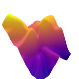
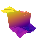
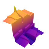
In this paper, we study SPs arising as infinitely wide limits of deep Stable NNs, i.e. deep NNs with Stable-distributed weights (Samoradnitsky and Taqqu, 1994). Stable distributions form a broad class of heavy tails or infinite variance distributions indexed by a parameter , and they are arguably the most natural generalization of the Gaussian distribution. The works Neal (1996) and Der and Lee (2006) first discussed the use of the Stable distribution for initializing deep NNs, leaving as an open problem the rigorous study of large-width asymptotic properties of deep Stable NNs. Empirical analyses in Neal (1996) show the following large-width phenomenon: while the contribution of Gaussian weights vanishes in the infinitely wide limit, Stable weights retain a non-negligible contribution, allowing them to represent “hidden features”. This phenomenon suggests a more flexible behaviour of NN’s weights with heavy tails, which results in infinitely wide SPs with a different behaviour than Gaussian SPs. In a classification setting, deep NNs trained with stochastic gradient descent result in heavy-tailed distributions for the weights, as a consequence of the training dynamics (Favaro et al., 2020; Fortuin et al., 2019; Hodgkinson and Mahoney, 2021). In such a setting, empirical analyses in Fortuin et al. (2019) show that the use of NN’s weights that are Stable-distributed leads to a higher classification accuracy, as it results in different path properties. See Figure 1 for (function) samples realized by wide fully-connected NNs whose weights are distributed as Stable distributions with decreasing , i.e. distributions with increasingly heavy tails. Recently, Li et al. (2021b) investigated the use of deep Stable NNs for image inverse problems when images contain sharp edges. Within this setting, the abrupt jumps allowed by the NN function mapping for lower values of result in a better matching prior for the problem of interest, and in superior performance in terms of inference.

Motivated by the recent interest in deep Stable NNs, we present a rigorous analysis of the large-width asymptotic behaviour of (fully connected) feed-forward deep Stable NNs, with depth , width and input-signals of dimension . We denote by the symmetric centered Stable distribution with stability parameter and scale parameter , and by the symmetric centered -dimensional Stable distribution with stability parameter and scale (finite) spectral measure on the unit sphere in . We refer to (Samoradnitsky and Taqqu, 1994, Chapter 1,2) for a detailed account of Stable distributions. The case is the Gaussian distribution, which is excluded from our analysis. The next theorem states our first main result, which extends Theorem 1 to deep Stable NNs. A preliminary version of the theorem appeared in (Favaro et al., 2020), though with a non-rigorous statement and proof.
Theorem 2 (Deep Stable NNs).
For any and let be a (input-signal) matrix, with being the -th row of , and for any and let: i) be a collection of i.i.d. random (weight) matrices, such that and for , where the ’s are i.i.d. as for ; ii) be a collection of i.i.d. random (bias) vectors, such that where the ’s are i.i.d. as for ; iii) be independent of . Moreover, for some , with , let be a continuous activation function such that
| (2) |
for every , and consider the NN of depth and width defined as follows
and
with , where is the -dimensional unit (column) vector, and denotes the element-wise application. For any , if is the sequence obtained by extending and to infinite i.i.d. arrays, then as jointly over the first layers
where is distributed as , with , with the spectral measure being defined as
and
| (3) |
with being the Euclidean norm in , where with being the Dirac measure and being the indicator function, where denotes the distribution of . Then, the limiting SP , as a process indexed by , is a Stable SP with parameter .
Critical to Theorem 2 is the assumption (2), which being stronger than (1) restricts the class of activation functions that lead to nontrivial infinitely wide limits. Such a restricted class, however, still includes popular activation functions, e.g. logistic, hyperbolic tangent and Gaussian. See Bordino et al. (2022) and Favaro et al. (2022) for infinitely wide limits of shallow Stable NNs with linear activation functions. As for Theorem 1, the non-triangular structure of the NN and the “joint growth” of the width over the NN’s layers make Theorem 2 a non-standard asymptotic problem, with the additional challenge of dealing with heavy tails distributions. The proof of Theorem 2 relies on the exchangeability of and, through de Finetti representation theorem, it exploits an inductive argument for the de Finetti measures over the NN’s layers; this is a novel approach of independent interest. Under the “sequential growth” of the width over the NN’s layers, the proof of Theorem 2 reduces to an application of a generalized central limit theorem Gnedenko and Kolmogorov (1954), which leads to the same limiting SP. Consistency or compatibility of the finite-dimensional distributions of the limiting Stable SP is also proved. As a refinement of Theorem 2, our second main result establishes sup-norm convergence rates of the rescaled deep Stable NN to the Stable SP, in both the “joint growth” setting and the “sequential growth” setting. In particular, such a result shows that the “joint growth” leads to a slower rate than the “sequential growth”, depending on the depth of the layer and . This is the first result on converge rates in the “joint growth” setting, providing the difference between the “sequential growth” and the “joint growth” settings.
1.2 Organization of the paper
The paper is structured as follows. In Section 2 we prove Theorem 2 and show consistency or compatibility of the finite-dimensional distributions of the limiting Stable SP, whereas in Section 3 we establish sup-norm convergence of the deep Stable NNs to the Stable SP under the “joint growth” and the “sequential growth” of the width over the NN’s layers. Section 4 contains a discussion of our results with respect to Bayesian inference, neural tangent kernel analysis via gradient descent and large-depth limits.
2 Proof of Theorem 2
Random variables are defined on a probability space , and we denote expectation by ; inequalities between conditional probabilities and between expectations must be interpreted as -a.s. For every and we denote by the sigma algebra generated by , by the trivial sigma algebra. Let and be the conditional expectation and the conditional distribution, respectively, given . For fixed , whenever . For fixed , is a filtration. We denote by the limit sigma-algebra, that is the sigma-algebra generated by . The conditional expectation, given , is denoted by . If then for
If is a -dimensional (row) random vector such that , then for a -dimensional (column) vector
If is a -dimensional (column) vector with all zeroes except a at the -th component, then the (-dimensional) -th element of is distributed as an -Stable distribution with stability and scale
Throughout this section, we most deal with -dimensional -Stable distributions with discrete spectral measure, that is with , and , for (Samoradnitsky and Taqqu, 1994, Chapter 2).
We start the proof by determining the distributions of the -dimensional (row) random vectors and for . We denote by the -th component of , that is . If is a -dimensional (column) vector, then
Therefore, , where
| (4) |
If is the -th component of the random vector , then with (Samoradnitsky and Taqqu, 1994, Chapter 2). Along similar lines, for each we write
Therefore, , where
| (5) |
Then, with (Samoradnitsky and Taqqu, 1994, Chapter 2).
Hereafter, we establish the infinitely wide limit of the . The proof exploits the exchangeability of and an inductive argument, over the NN’s layers, for the directing (de Finetti) random probability measure of . For , by definition, the random vectors are i.i.d. according to the probability measure , where is defined in (4). Then, as , converges weakly to . For , the random vectors are conditionally i.i.d. given , with (random) probability measure , where is defined in (5). Given , the sequence is conditionally independent of . It follows that are conditionally i.i.d., given , with (random) probability measure . Before stating the induction hypothesis, we give a preliminary result.
Lemma 3.
Let be such that and . Then, for each and every
Proof.
Since and , then there exists that satisfies the conditions in the statement. Moreover, since is an -stable distribution and since , then . The thesis follows by noticing that, since , then there exist such that it holds true
∎
Now, we present the induction hypothesis over the NN’s layers, which is critical to prove Theorem 2. In particular, it is assumed that, for every index and for as specified in Lemma 3, as
| (6) |
| (7) |
and
| (8) |
with being the and with being specified by the recurrence relation (3), with being defined in (4). Note that the both the integrals that appear in Equation (7) and Equation (8) are finite by Lemma 3 and since . The induction hypothesis is trivially true for since . Note that, according to the induction hypothesis, as , has a deterministic limit at , for every . The proof of Theorem 2 is presented in three steps. First, it is shown that (6), (7) and (8) hold true for . Then for each we show that
| (9) |
as , where is distributed as , with being defined in (3). Then, as , the weak convergence of to follows directly by combining (9) with some standard arguments that exploit the finite-dimensional projections of (Billingsley, 1999).
2.1 Induction step
We start by proving the induction hypothesis given by the combination of Equation (6), Equation (7) and Equation (8). In particular, let be a -dimensional (column) vector, then we can write the following:
| (10) | ||||
Then (6), with , follows by combining the conditional characteristic function (10) with the following lemma.
Proof.
We prove Equation (6) by combining the conditional characteristic function (10) with (6), (7) and (8) for , and then by Lemma 3 and Lemma 4. By combining (10) with Lemma 3, we write
Now, by means of a direct application of Lagrange theorem, there exists a random variable such that
Now, since by Lemma 4,
as , then
as , by (8), Lemma 4, and since , as . By (Blackwell and Dubins , 1962, Theorem 2),
| (11) |
as , where the last equality holds true since is deterministic. Therefore, , converges a.s. in the weak topology to , thus proving the induction step for (6), where we set
Now, we prove that Equation (7) holds true for . The proof is based on a uniform integrability argument. Since converges a.s. to , with respect to the weak topology, then, for every ,
Denoting by a random variable distributed according to , we can write, for every ,
It follows that, for every , the functional is a.s. uniformly integrable with respect to , that is
To prove it, fix such that converges weakly to , as , and let and be random vectors defined on a probability space with distribution and , respectively. Then, under , the sequence converges in distribution, as , to and also
By uniform integrability,
as . Thus, is a.s. uniformly integrable with respect to , for . Since for some
then is a.s. uniformly integrable with respect to . Since converges a.s.to , then converges a.s. to . This proves the induction step for (7). Finally, we prove that Equation (8) holds true for . In particular, we observe that . Then, is also a.s. uniformly integrable with respect to . Equation (8) with follows from this and (6) with . This completes the proof of the induction hypothesis.
2.2 Weak convergence of
We prove Equation (9). In particular, by means of (2.1) and dominated convergence theorem, which is applied to the sequence of uniformly bounded random variables, we can write
That is, converges weakly, as , to distributed as , for each , where
with being the distribution of , for . This result completes the proof of (9).
2.3 Weak convergence of
By Cramér-Wold theorem (Billingsley, 1999) the convergence of to some limit is equivalent to convergence on all possible linear projections of to the corresponding real-valued random variable. Let and let such that and . Then, we consider the linear projection
where we set for . Then, we can write that
That is,
where is a random vector with symmetric -stable distribution and spectral measure of the form
Along lines similar to the proof of the large asymptotics for the -th coordinate , we can show that
as . That is, the linear projection converges weakly, as , to where the are i.i.d. according to , where we set
with being the distribution of , for any . Therefore, by means of Cramér-Wold theorem, converges weakly, as , to the Stable SP , as a process indexed by , whose distribution is . This completes the proof of Theorem 2
As a complement to the proof of Theorem 2, we show the consistency or compatibility of the finite-dimensional distributions of the Stable SP . In particular, proceeding by induction, we write
and, for ,
Now, we define , , and . Moreover, for every , we define a measure as follows
Then
Therefore, the consistency of the finite-dimensional distributions holds for . Now suppose that the consistency holds true for every . In particular, has distribution . Then, we can write that
which proves consistency or compatibility of the finite dimensional distributions for of the Stable SP .
3 Sup-norm convergence rates
In this section, we refine Theorem 2 by establishing sup-norm convergence rates of the deep Stable NN to the Stable SP , under both the setting of “sequential growth” and “joint growth” of the width over the NN’s layers. Throughout this section we make the following assumptions:
| (12) |
and
| (13) |
3.1 The “joint growth” setting
The “joint growth” setting consists in assuming that, for any , the width simultaneously over the first layers. We recall from Section 2 that and for any , where and are defined in (4) and (5), respectively. In particular, and are finite random measures with (random) total masses given by
and
for , respectively. We recall from Theorem 2 that for , where is a finite measure displayed in (3). Under the assumption (12), it holds that
and
| (14) |
for . Such a condition, together with the following lemma, allows to give an explicit uniform bound for the tails of the Stable distributions that are involved in the definition of the deep Stable NN.
Lemma 5 (Byczkowski et al. (1993)).
Let be a -dimensional random vector distributed as a symmetric centered -stable distribution with spectral measure . If
then for every whenever is such that .
To establish sup-norm convergence rates, it is useful to consider linear transformations of the random vectors and (Samoradnitsky and Taqqu, 1994, Chapter 2). In particular, if is a -dimensional (column) vector then
-
i)
, where
-
ii)
, where
-
iii)
, where
We denote by the Lebesgue measure on . The next lemmas are critical to establish sup-norm convergence rates, as they show that the distributions and are absolutely continuous with respect to the Lebesgue measure. The next two lemmas deal with the distribution of .
Lemma 6 (Nolan (2010)).
Let and be -dimensional random vectors distributed as symmetric -stable distributions with spectral measures and , satisfying
respectively. Then, the corresponding density functions and exist and are such that
Lemma 7.
Proof.
If , then absolute continuity of the distribution of follows from Lemma 6. Since are continuous on , the minimum is attained. Thus, it is sufficient to show that
| (16) |
We prove (16) by induction on the NN’s layers. If there exists a vector such that , then it holds that and for every . On the other hand, since spans , then there exists such that . Thus which contradicts . Thus (15) holds true for and the distribution of is absolutely continuous. Now suppose that (15) holds true so that the distribution of is absolutely continuous. Since is continuous and strictly increasing, then the distribution of is also absolutely continuous. Thus, for every , , which implies that . Thus, for every . ∎
By Lemma 7, is absolutely continuous with respect to the Lebesgue measure, for , and we denote by its density function. The next three lemmas deal with the distribution of .
Proof.
Under (12) the assumptions of Theorem 2 hold true. Its proof shows that, for every , the conditional distribution of , given is and converges a.s. in the weak topology, to the law of , which is . As a consequence, by ii) and iii) above, for every ,
Since the function is continuous, the thesis follows. ∎
Lemma 9.
For every and every
Proof.
We start by defining . Since is compact, then there exist and in such that: for every there exists such that . Now, let for . Then, and for every it holds that
for every . Now, fix and let . Moreover, let be such that . Then, if , for every , we can write
On the other hand, if then by the Lagrange theorem there exists , with , such that we can write
Thus
∎
We define the set . Then, it holds that and for every there exists such that
From Lemma 6, for every , is absolutely continuous with respect to the Lebesgue measure, for . We denote by a version of the (random) density function of , with respect to the Lebesgue measure. We can extend the definition of to every and every . The next theorem establishes the convergence rate of to .
Theorem 11 (The “joint growth” setting).
Proof.
We restrict to the set . Similarly to the proof of Theorem 2, we consider induction over the NN’s layers . In particular, by Lemma 6 it holds that
with . Since for large enough, the measures and are bounded by (14) and bounded away from zero by Lemma 7 and Lemma 10, proving that converges in probability to zero is equivalent to proving that converges in probability to zero. In particular, for , we can write
By means of (von Bahr and Esseen, 1965, Theorem 2),
as . Now, recall that the convergence in in , with being the Borel sigma algebra of , implies the convergence in . Therefore, we can write
as , which implies
| (18) |
as . This completes the proof for . Now, as the main induction hypothesis, we assume that
as , for some . By (17), there exists such that . Then, we write
| (19) | ||||
We consider the two terms on the right-hand side of (19). With regards to the first term, by Theorem 2 in von Bahr and Esseen (1965),
as . Since convergence in in implies the convergence in ,
as , which implies
| (20) |
as . For the second term on the right-hand side of (19), by Lemma 5 with ,
as , since we have . This completes the proof. ∎
Theorem 11 provides a refinement of Theorem 2 by establishing the sup-norm convergence rate of a deep Stable NNs to a Stable SPs, in the “joint growth” setting. As in Theorem 2, the proof in the “joint growth” setting requires the use of an induction argument or induction hypothesis over the NN’s layers . In particular, by means of such an induction argument, it is shown how the convergence rate is affected by the depth of the layer, i.e. , and by the dimension of the input That is,
| (21) |
and for
| (22) |
Then, according to (21) and (22), the assumption of the “sequential growth” setting implies two critical effects on the convergence rates: i) for any , the deeper the layer in the NN the slower the convergence rate; ii) for each fixed , the larger the dimension of the inuput the slower the convergence rate. Such a behaviour is completely determined by the assumption of the “joint growth” setting, and a different behaviour is expected under the assumption of the “sequential growth” setting.
3.2 The “sequential growth” setting
The “sequential growth” setting consists in assuming that, for any , the width one layer at a time. To deal with such a setting, we consider the deep Stable NN defined as follows
and
where is a sequence of -dimensional (row) random vectors such that, as , it holds that
The distribution of coincides with the distribution of the Stable SP in Theorem 2. Under the “sequential growth” setting, the study of convergence rates of to reduces to the study of convergence rates of , which is a simpler problem.
Let denote the sigma algebra generated by , for any , and let denote the trivial sigma algebra. To establish sup-norm convergence rates, it is useful to consider linear transformations of the random vectors and . If is a -dimensional (column) vector then
-
i)
, where
-
ii)
, where
-
iii)
, where
Under (12),
| (23) |
for D, with defined as in (14). We denote by and the conditional expectation and the conditional distribution, respectively, given , and by the Lebesgue measure on . Assuming that (12) and (13) hold, along lines similar to that of Lemma 8, Lemma 9 and Lemma 10 we have
| (24) |
and
| (25) |
for every , every with , and every . By Lemma 6, the probability measure is absolutely continuous with respect to the Lebesgue measure, and we denote by its density function. Moreover, for every , is absolutely continuous with respect to the Lebesgue measure, for . In particular, we denote by a version of the density function of . We can extend the definition of to every and every . The next theorem establishes the convergence rate of to .
Theorem 12 (The “sequential growth” setting).
Proof.
We restrict to the set . Now, since and , for , by Lemma 6, it is sufficient to show that
| (26) |
as . The measures and are bounded by (14); moreover, they are bounded away from zero, as shown in (24) and (25). Accordingly, (26) is equivalent to the following
| (27) |
as . By ii) and iii) above,
and by (von Bahr and Esseen, 1965, Theorem 2),
as . Now, the convergence in in , with being the Borel sigma algebra of , implies the convergence in . Accordingly, we can write the following
as , which implies that
as . This completes the proof. ∎
Theorem 12 provides an interesting complement to Theorem 11, as it highlights a critical difference between the “joint growth” and the “sequential growth” settings. Differently from the “joint growth” setting, the “sequential growth” setting does not require the use of an induction argument over the NN’s layers , as in the study of the convergence rate at layer it is assumed that the layer has already reached its limit. In particular, Theorem 12 shows how in the “sequential growth” setting the convergence rate is not affected by the the depth of the layer, i.e. , or the dimension of the input. That is,
| (28) |
for every . According to (28), the assumption of the “sequential growth” setting implies that the convergence rate is constant with respect to the depth of the layer and the dimension of the input. While at the level of the infinitely wide limit in Theorem 2 there are no difference between the “joint growth” and the “sequential growth” settings, as both settings lead to the same infinitely wide Stable process, our results show how a difference between these settings appears at the refined level of convergence rate. To the best of our knowledge, our work is the first to provide a quantitative result on the difference between the “joint growth” setting and the “sequential growth” setting.
4 Discussion
We discuss the potential of our results with respect to to Bayesian inference, gradient descent via neural tangent kernels and depth limits, and we present open challenges in large-width asymptotics for deep Stable NNs.
4.1 Bayesian inference
From Theorem 1, we know that infinitely wide deep Gaussian NNs give rise to i.i.d. centered Gaussian SPs at every layer . Now, assume that we are given a training dataset of distinct observations where each is a -dimensional input and its corresponding scalar output. Then, we are interested in determining the conditional distributions of the limiting Gaussian SPs over a set of test input values given the training dataset, that is the distribution of
| (29) |
where and we indexed training observations from to , test inputs from to . Theorem 1 establishes that the covariance matrices of the limiting Gaussian SPs over all inputs, one for each layer , can be computed via a recursion over such layers. Lee et al. (2018) proposes an efficient quadrature solution that keeps the computational requirements manageable for an arbitrary activation . Once the covariance matrix over all inputs for a given layer is available, standard results on multivariate Guassian vectors establish that the distribution of (29) is multivariate Gaussian, whose mean vector and covariance matrix is obtainable via simple (but potentially costly) algebraic manipulations (Rasmussen and Williams, 2006).
In the context of deep Stable NNs, computing the distribution of (29) is a more challenging task with respect to deep Gaussian NNs. Note that it is possible to approximately simulate from the distribution of . In particular, since is a discrete measure then exact simulations algorithms are available with a computational cost of per sample (Nolan, 2008; Samoradnitsky and Taqqu, 1994). Therefore, we generate samples , , in , and use these to approximate with where
We can repeat this procedure by generating (approximate) random samples , with a cost of , that in turn are used to approximate and so on. The sequential discretization of the spectral measure to perform approximate sampling is not advantageous. Such a procedure can be shown to be equivalent (in distribution) to sequentially sampling over the layers of the finite NN of width . In any case, we still have the problem of computing a statistic of (29) or sampling from it, to perform prediction. In general, performing inference with the Stable SPs of Theorem 2 remains an open problem.
4.2 Neural tangent kernel
In Section 4.1 we reviewed how the interplay between deep Gaussian NNs and Gaussian SPs allows to perform Bayesian inference on the infinitely wide SP. This corresponds to a “weakly-trained” regime, in the sense that the posterior mean predictions of (29) are equivalently obtained by assuming a quadratic loss function, and then fitting only the final linear layer of the NN with gradient flow, i.e. gradient descent with infinitesimal learning rate (Arora et al., 2019). This result thus establishes an equivalence between a specific training setting for deep Gaussian NN and a kernel regression. Differently, the works Jacot et al. (2018); Lee et al. (2019); Arora et al. (2019) consider “fully-trained” deep Gaussian NNs, in the sense that all the layers are trained jointly, still under the same quadratic loss and gradient flow. It is shown that as the width of the NN goes to infinity, the point predictions are still equivalent to that of a kernel regression, though with respect to a different kernel, which is referred to as the neural tangent kernel. A key assumption in the derivation of the neural tangent kernel is that the gradients are not computed with respect to the standard model parameters, i.e. the weights and biases entering the affine transforms. Instead, they are re-parametrized gradients which are computed with respect to weights distributed as standard Gaussian distributions, with any scaling (standard deviation) applied as a further multiplication. Recently, Favaro et al. (2022) introduced an analogous equivalence in the context of “fully-trained” shallow Stable NNs with a ReLU activation function, showing that the underlying kernel regression is with respect to an -Stable random kernel. We believe that it would be of interest to study whether the work of Favaro et al. (2022) can be extended to the context of deep -Stable NNs with a general activation function, i.e. linear and sub-linear.
4.3 Depth limits
In the context of deep Gaussian NNs, information propagation investigates the evolution over depth of the covariance matrix recursion in Theorem 1 (Poole et al., 2016; Schoenholz et al., 2017; Hayou et al., 2019). In particular, following the notation and the assumptions of Theorem 1, it is shown that the positive quadrant is divided into two regions: i) a stable phase; ii) a chaotic phase. Assuming for simplicity , in the stable phase the limiting Gaussian SP correlation between any two distinct inputs tends to as the depth grows unbounded, and the limiting Gaussian SP concentrates on constant functions. Under the same assumption , in the chaotic phase this correlation converges to a random variable, and the limiting Gaussian SP is almost everywhere discontinuous. Hayou et al. (2019) investigates the case where is on the curve separating the stable phase from the chaotic phase, which is typically referred to as the edge of chaos curve. On such a curve, it is shown that the behavior is qualitatively similar to that of the stable phase, but with a lower rate of convergence with respect to depth. Thus, in all cases, the distribution of the limiting Gaussian SP eventually collapse to degenerate and inexpressive distributions as the depth increases.
It would be interesting to investigate the role on the Stable distribution, with , in the edge of chaos phenomenon. It seems difficult to escape the curse of depth under i.i.d. distributions for the weights, though it might be the case that Stable distributions, with their not-uniformly-vanishing relevance at unit level Neal (1996), allow to slow down the rate of convergence to the limiting regime. For deep Gaussian NNs of finite width, a way to avoid the curse of depth is to shrink the distribution of the NN’s weights as the total number of layers increases. This idea has been explored in Cohen et al. (2021), with the critical result that as goes to infinity the finite-width NN converges to the solution of a stochastic differential equation (SDE). We conjecture that, under appropriate scaling, the same approach applied to a NN whose weights are distributed as Stable distributions would result in converge to the solution of a Levy-driven stochastic differential equation. A more recent line of research focuses on taking joint limits in width and depth (Li et al., 2021). Here, the theory is less developed, and a formal result among the lines of Theorem 1 is lacking. However, the partial results that have been obtained so far hint at a class of limiting SPs that might better capture the properties of finitely-sized NNs. Interestingly such limiting SPs are not Gaussian SPs. Therefore, it would be of interest to investigate some extensions of Theorem 2 under the more flexible scenario where both the width and depth are allowed to grow, possibly at different rates.
Acknowledgement
The authors are grateful to three anonymous Referees for all their comments, corrections, and numerous suggestions that improved remarkably the paper. Stefano Favaro received funding from the European Research Council (ERC) under the European Union’s Horizon 2020 research and innovation programme under grant agreement No 817257. Stefano Favaro gratefully acknowledge the financial support from the Italian Ministry of Education, University and Research (MIUR), “Dipartimenti di Eccellenza” grant 2018-2022.
References
- Aitken and Gur-Ari (2020) Aitken, K. and Gur-Ari, G. (2020). On the asymptotics of wide networks with polynomial activations. Preprint: arXiv:2006.06687.
- Andreassen and Dyer (2020) Andreassen, A. and Dyer, E. (2020). Asymptotics of wide convolutional neural networks. Preprint: arXiv:2008.08675.
- Antognini (2019) Antognini, J.M. (2019). Finite size corrections for neural network gaussian processes. Preprint: arXiv:1908.10030.
- Arora et al. (2019) Arora, S., Du, S.S., Hu, W., Li, Z., Salakhutdinov, R.R. and Wang, R. (2019). On exact computation with an infinitely wide neural net. In Advances in Neural Information Processing Systems.
- Basteri and Trevisan (2022) Basteri, A. and Trevisan, D. (2022). Quantitative Gaussian approximation of randomly initialized deep neural networks Preprint arXiv:2203.07379.
- Billingsley (1999) Billingsley, P. (1999). Convergence of probability measures. Wiley-Interscience.
- Blackwell and Dubins (1962) Blackwell, D. and Dubins, L. (1962) Merging of opinions with Increasing Information. The Annals of Mathematical Statistics 33, 882 – 886.
- Blum et al. (1958) Blum, J.R., Chernoff, H., Rosenblatt, M. and Teicher, H. (1958). Central limit theorems for interchangeable processes. Canadian Journal of Mathematics 10, 222-229.
- Bordino et al. (2022) Bordino, A., Favaro, S. and Fortini (2022). Infinite-wide limits for Stable deep neural networks: sub-linear, linear and super-linear activation functions. Preprint available upon request.
- Byczkowski et al. (1993) Byczkowski, T., Nolan, J.P. and Rajput, B. (1993). Approximation of multidimensional Stable densities. Journal of Multivariate Analysis 46, 13–31.
- Cohen et al. (2021) Cohen, A., Cont, R., Rossier, A. and Xu, R. (2021). Scaling properties of deep residual networks. In International Conference on Machine Learning.
- Der and Lee (2006) Der, R. and Lee, D. (2006). Beyond Gaussian processes: on the distributions of infinite networks. In Advances in Neural Information Processing Systems.
- Eldan et al. (2021) Eldan, R., Mikulincer, D. and Schramm, T. (2021). Non-asymptotic approximations of neural networks by Gaussian processes. In Conference on Learning Theory.
- Favaro et al. (2020) Favaro, S., Fortini, S. and Peluchetti, S. (2020). Stable behaviour of infinitely wide deep neural networks. In International Conference on Artificial Intelligence and Statistics.
- Favaro et al. (2022) Favaro, S., Fortini, S. and Peluchetti, S. (2022). Neural tangent kernel analysis of shallow -Stable ReLU neural networks. Preprint arXiv:2206.08065.
- Fortuin et al. (2019) Fortuin, V., Garriga-Alonso, A., Wenzel, F., Ratsch, G, Turner, R.E., van der Wilk, M. and Aitchison, L. (2020). Bayesian neural network priors revisited. In Advances in Neural Information Processing Systems.
- Garriga-Alonso et al. (2018) Garriga-Alonso, A., Rasmussen, C.E. and Aitchison, L. (2018). Deep convolutional networks as shallow Gaussian processes. In International Conference on Learning Representation.
- Gnedenko and Kolmogorov (1954) Gnedenko, B.V. and Kolmogorov, A.N. (1954). Limit distributions for sums of independent random variables. Addison-Wesley.
- Hayou et al. (2019) Hayou, S. and Doucet, A. and Rousseau, J. (2019). On the impact of the activation function on deep neural networks training. In International Conference on Machine Learning.
- Hazan and Jaakkola (2015) Hazan, T. and Jaakkola, T. (2015). Steps toward deep kernel methods from infinite neural networks. Preprint: arXiv:1508.05133.
- Hodgkinson and Mahoney (2021) Hodgkinson, L. and Mahoney, M. (2021). Multiplicative noise and heavy tails in stochastic optimization. In International Conference on Machine Learning.
- Jacot et al. (2018) Jacot, A., Gabriel, F, and Hongler, C. (2018). Neural tangent kernel: convergence and generalization in neural networks. In Advances in Neural Information Processing Systems.
- Joe and Kuo (2008) Joe, S. and Kuo, F.Y. (2008). Notes on generating Sobol sequences. ACM Transactions on Mathematical Software 29, 49–57.
- Klukowski (2021) Klukowski, A. (2021). Rate of convergence of polynomial networks to Gaussian processes Preprint arXiv: 2111.03175.
- LeCun et al (2015) LeCun, Y., Bengio, Y. and Hinton, G. (2015). Deep learning. Nature 521, 436–444.
- Lee et al. (2020) Lee, J., Schoenholz, S. Pennington, J., Adlam, B., Xiao, L., Novak, R. and Sohl-Dickstein, J. (2020). Finite versus infinite neural networks: an empirical study. In Advances in Neural Information Processing Systems.
- Lee et al. (2018) Lee, J., Sohldickstein, J., Pennington, J., Novak, R., Schoenholz, S. and Bahri, Y. (2018). Deep neural networks as Gaussian processes. In International Conference on Learning Representation.
- Lee et al. (2019) Lee, J., Xiao, L., Schoenholz, S., Bahri, Y., Sohl-Dickstein, J. and Pennington, J. (2019). Wide neural networks of any depth evolve as linear models under gradient descent. In Advances in Neural Information Processing Systems.
- Li et al. (2021b) Li, C., Dunlop, M. and Stadler, G. (2021). Bayesian neural network priors for edge-preserving inversion. Preprint arXiv:2112.10663.
- Li et al. (2021) Li, M.B., Nica, M. and Roy, D.M. (2021). The future is log-Gaussian: ResNets and their infinite-depth-and-width limit at initialization. Preprint arXiv:2106.04013.
- Matthews et al. (2018) Matthews, A.G., Rowland, M., Hron, J., Turner, R.E. and Ghahramani, Z. (2018). Gaussian process behaviour in wide deep neural networks. In International Conference on Learning Representations.
- Neal (1996) Neal, R.M. (1996). Bayesian learning for neural networks. Springer.
- Nolan (2008) Nolan, J.P. (2010). An overview of multivariate Stable distributions. Preprint, Department of Mathematics and Statistics at American University.
- Nolan (2010) Nolan, J.P. (2010). Metrics for multivariate Stable distributions. Banach Center Publications 90, 83–102.
- Novak et al. (2018) Novak, R., Xiao, L., Bahri, Y., Lee, J., Yang, G., Hron, J., Abolafia, D., Pennington, J. and Sohldickstein, J. (2018). Bayesian deep convolutional networks with many channels are Gaussian processes. In International Conference on Learning Representation.
- Poole et al. (2016) Poole, B., Lahiri, S., Raghu, M., Sohl-Dickstein, J. and Ganguli, S. (2016). Exponential expressivity in deep neural networks through transient chaos. In Advances in Neural Information Processing Systems.
- Rasmussen and Williams (2006) Rasmussen, C.E. and Williams, C.K.I. (2006). Gaussian Processes for Machine Learning. MIT Press.
- Samoradnitsky and Taqqu (1994) Samoradnitsky, G. and Taqqu, M.S (1994). Stable non-Gaussian random processes: stochastic models with infinite variance. Chapman and Hall/CRC.
- Schoenholz et al. (2017) Schoenholz, S., Gilmer, J., Ganguli, S. and Sohl-Dickstein, J. (2017). Deep information propagation. In International Conference on Learning Representation.
- von Bahr and Esseen (1965) von Bahr, B. and Esseen, C. (1965). Inequalities for the th absolute moment of a sum of random variables. Annals of Mathematical Statistics 1, 299–303.
- Williams (1997) Williams, C.K. (1997). Computing with infinite networks.. In Advances in Neural Information Processing Systems.
- Yang (2019) Yang, G. (2019). Scaling limits of wide neural networks with weight sharing: Gaussian process behavior, gradient independence, and neural tangent kernel derivation. Preprint: arXiv:1902.04760.
- Yang (2019a) Yang, G. (2019). Tensor programs I: wide feedforward or recurrent neural networks of any architecture are Gaussian processes. Preprint: arXiv:1910.12478.