Investigating the Pilot Point Ensemble Kalman Filter for geostatistical inversion and data assimilation

Abstract

Parameter estimation has a high importance in the geosciences. The ensemble Kalman filter (EnKF) allows parameter estimation for large, time-dependent systems. For large systems, the EnKF is applied using small ensembles, which may lead to spurious correlations and, ultimately, to filter divergence. We present a thorough evaluation of the pilot point ensemble Kalman filter (PP-EnKF), a variant of the ensemble Kalman filter for parameter estimation. In this evaluation, we explicitly state the update equations of the PP-EnKF, discuss the differences of this update equation compared to the update equations of similar EnKF methods, and perform an extensive performance comparison. The performance of the PP-EnKF is tested and compared to the performance of seven other EnKF methods in two model setups, a tracer setup and a well setup. In both setups, the PP-EnKF performs well, ranking better than the classical EnKF. For the tracer setup, the PP-EnKF ranks third out of eight methods. At the same time, the PP-EnKF yields estimates of the ensemble variance that are close to EnKF results from a very large-ensemble reference, suggesting that it is not affected by underestimation of the ensemble variance. In a comparison of the ensemble variances, the PP-EnKF ranks first and third out of eight methods. Additionally, for the well model and ensemble size 50, the PP-EnKF yields correlation structures significantly closer to a reference than the classical EnKF, an indication of the method’s skill to suppress spurious correlations for small ensemble sizes.

Accepted for publication in Advances in Water Resources. Copyright 2021 Elsevier. Further reproduction or electronic distribution is not permitted.

1 Introduction

Predictions of groundwater flow, mass transport and heat transport are strongly influenced by subsurface hydraulic properties like the hydraulic conductivity used in the groundwater flow equation. Unfortunately, hydraulic conductivity is often strongly heterogeneous in space with limited measurement information. Starting in the 1970’s, many studies worked on estimating these properties with the help of inverse algorithms. The 1980’s saw a transition towards stochastic inverse methods (Kitanidis and Vomvoris, 1983) and, since the 1990’s, methods were formulated for generating multiple equally likely solutions to the groundwater inverse problem (Gómez-Hernández et al., 1997). In the 2000’s, the ensemble Kalman filter method (EnKF, Evensen, 1994, Burgers et al., 1998) became popular. In its parameter estimation version, it also calculates equally likely solutions to the groundwater inverse problem, but avoids the formulation of numerical derivatives that were needed in many inversion methods used until then (e.g., Chen and Zhang, 2006, Hendricks Franssen and Kinzelbach, 2008, Nowak, 2009). An overview on the groundwater inverse literature including comparison of methods can be found in Carrera et al. (2005), Hendricks Franssen et al. (2009) and Zhou et al. (2014).

The ensemble Kalman filter is a sequential method, which is suited for large and non-linear numerical models. When the EnKF is used for parameter estimation, parameters are updated at a sequence of observation times according to observation data and covariance information from an ensemble of stochastic realizations. After assimilation of all measurement data, the ensemble is used to approximate the full posterior probability density distribution. However, problems such as filter inbreeding and ultimately filter divergence have been diagnosed for the EnKF for small ensemble sizes (Hamill et al., 2001).

For many EnKF methods, sampling errors of the covariances between dynamic variables and parameters are responsible for filter divergence. A number of EnKF methods have been proposed and applied to tackle such shortcomings of the EnKF related to small ensemble sizes. Two examples are the local EnKF (Hamill et al., 2001) and the hybrid EnKF (Hamill and Snyder, 2000). In the local EnKF (also called covariance localization), covariances are restricted to the vicinity of observations. In the hybrid EnKF, the full covariance matrix is a weighted sum of the ensemble covariance matrix, which is the covariance of the classical Kalman filter update, and a fixed covariance matrix, which is defined before the assimilation, according to prior knowledge and modeled the same way as the initial covariance matrix. Additional EnKF methods include the damped EnKF (Hendricks Franssen and Kinzelbach, 2008), and the iterative EnKF (Sakov et al., 2012). In the damped EnKF, the proposed EnKF update is multiplied by a damping factor to reduce the update of the parameters. This approach reduces problems with filter inbreeding. In contrast, the iterative EnKF restarts the whole assimilation after every EnKF update, thereby reducing numerical instabilities connected to nonlinear model equations.

Further developments include the application of an ensemble smoother (Evensen, 2000, Chen and Oliver, 2011, Emerick and Reynolds, 2013, Cosme et al., 2012), and, in particular, an iterative version of this smoother (Bocquet and Sakov, 2013). Crestani et al. (2013) compare ensemble smoothers to the EnKF in a tracer test assimilation, concluding that the EnKF outperforms smoothers in this scenario. Additionally, the iterative EnKF has been tested for additive model error (Sakov et al., 2018). A disadvantage of iterative approaches is the strong increase in needed compute time. Also, adaptive covariance inflation of the EnKF has been extensively tested recently (Raanes et al., 2019). Another line of research focuses on the model equations and reducing computational effort by combining EnKF variants with methods such as principal component analysis and reduced basis (Kang et al., 2017, Pagani et al., 2017, Xiao et al., 2018). However, these methods do not tend to reduce problems with spurious correlations and filter inbreeding.

In this work, we explicitly formulate and extensively test the pilot point ensemble Kalman filter (PP-EnKF) as an alternative approach for parameter estimation. The PP-EnKF was initially introduced, sketched and tested in a small suite of four tests by Heidari et al. (2013), using a 50-member ensemble in a petroleum reservoir model. The result was that this method yielded larger RMSE than classical EnKF, getting better as the number of pilot points approached the full set of parameters. On the other hand, spatial variability was found to be better preserved by this method compared to the classical EnKF. Similar results were obtained by Crestani (2013, Chapter 4). In a second performance comparison of the same method, Tavakoli et al. (2013) tested the PP-EnKF from Heidari et al. (2013) against the EnKF, ensemble smoothers and null-space Monte Carlo methods using a 200-member ensemble in a multiphase model. In this comparison, the PP-EnKF performed well, yielding the smallest RMSE for the estimated logarithmic permeability field. In (Tavakoli et al., 2013), the spread of the estimated EnKF-PP field was actually smaller than for the other ensemble methods, a result that is contradictory to the findings in (Heidari et al., 2013). This discrepancy makes it interesting to investigate this promising method further, give an explicit statement of the mathematical formulae and an extensive investigation of the performance of our PP-EnKF.

The specific contribution of this paper is twofold. First, the statement of the explicit mathematical formulae of the PP-EnKF and its non-ensemble version, and second, an extensive testing of the PP-EnKF in a large comparison. The original publication (Heidari et al., 2013) contains no explicit mathematical formulae, while our investigation starts at the classical Kalman filter, shows the differences of the classical Kalman filter and a pilot point Kalman filter and, finally, translates the derivation to the corresponding ensemble methods obtaining the full PP-EnKF filter equations and their ideal (linearized) estimation variance. This derivation provides a rigorous mathematical and statistical foundation to the method, and provides insights on its behavior in various situations. Regarding the testing, our performance tests of the PP-EnKF are based on a much larger test set compared to earlier tests in (Heidari et al., 2013) and (Tavakoli et al., 2013). Our statistically independent repetition of performance tests includes RMSEs and overall standard deviations from 1,000 synthetic experiments and, additionally, the comparison of full correlation fields from 10 synthetic experiments. The latter is to assess the ability of the PP-EnKF to suppress spurious correlations.

In Section 2, the PP-EnKF is introduced with a focus on the differences between the classical EnKF and the PP-EnKF. In Section 3, the two setups for synthetic experiments and the performance evaluation measures are detailed. In Section 4, we present results of the comparison of the PP-EnKF to the other seven EnKF variants for the two parameter estimation setups. Section 5 contains a brief conclusion.

2 Pilot Point Ensemble Kalman Filter

In this section, the ensemble equations of the PP-EnKF are introduced by first defining the simpler equations of the pilot point Kalman filter (PP-KF). The PP-KF is obtained by splitting the state vector of the Kalman filter into dynamic variables, pilot point parameters and non-pilot point parameters. The Kalman update is applied to dynamic variables and pilot point parameters. The remaining parameter values are updated by a kriging interpolation of the update. In the next step, the ensemble versions of the equations are formulated, resulting in the PP-EnKF. We show how the update of the PP-EnKF, which is a mixture of an update and an interpolation of this update, differs from the update in the classical EnKF. Additionally, we compare the formulation of the PP-EnKF to the formulations of the local EnKF and the hybrid EnKF in order to show that, while aiming at the same goal of suppressing spurious correlations, the PP-EnKF provides a useful alternative.

2.1 Kalman Filter and Ensemble Kalman Filter

Before the PP-EnKF is presented, we quickly recall the equations for the Kalman filter (Kalman et al., 1960) and the ensemble Kalman filter (Evensen, 1994). One advantage of the Kalman filter is that no adjoint equations are needed in its formulation. The PP-EnKF differs from the EnKF only in the update equation. A full account of the EnKF can be found in Evensen (2003) and also in our earlier work, where we provide more detail on EnKF variants and comparison methods (Keller et al., 2018).

The unperturbed Kalman filter forward equation for the mean of the state vector is given by

$$\mathbf{x}^{f}=\mathbf{M}\mathbf{x}^{b},$$ (1)

where the vector $\mathbf{x}^{b}\in R^{n_{s}}$ is either the initial mean state vector or, in later time steps, the assimilated mean state vector from the previous assimilation step. The forward computation is represented by the matrix $\mathbf{M}\in R^{n_{s}\times n_{s}}$. We define $n_{s}$ as the size of the state vector. The state vector consists of both dynamic variables and static parameters. $\mathbf{x}^{f}\in R^{n_{s}}$ is the state vector of predictions computed by the forward simulation. In the Kalman filter, a second forward equation for the covariance matrix is given by

$$\mathbf{P}=\mathbf{M}\mathbf{P}^{b}\mathbf{M}^{T},$$ (2)

where $\mathbf{P}^{b}\in R^{n_{s}\times n_{s}}$ is either the initial covariance matrix or the assimilated covariance matrix from the previous assimilation step. $\mathbf{P}\in R^{n_{s}\times n_{s}}$ is the covariance matrix of the predicted state vector. The predictions $\mathbf{x}^{f}$ and $\mathbf{P}$ serve as input to the update equation of the Kalman filter.

The Kalman filter update equation for the mean of the state vector is given by

$$\mathbf{x}^{a}-\mathbf{x}^{f}=\mathbf{P}\mathbf{H}^{T}\left(\mathbf{H}\mathbf{P}\mathbf{H}^{T}+\mathbf{R}\right)^{-1}\left(\mathbf{d}-\mathbf{H}\mathbf{x}^{f}\right)\,.$$ (3)

On the left-hand side of this equation, $\mathbf{x}^{a}\in R^{n_{s}}$ is the state vector after the Kalman filter update. $\mathbf{x}^{f}\in R^{n_{s}}$ is the state vector of predictions computed by the forward simulation. On the right-hand side of the equation, $\mathbf{d}\in R^{n_{m}}$ is the vector of measurements, where $n_{m}$ is the number of measurements. $\mathbf{R}\in R^{n_{m}\times n_{m}}$ is the measurement error matrix and $\mathbf{H}\in R^{n_{m}\times n_{s}}$ is the measurement operator. The measurement operator maps the state vector to the measurements.

The update equation for the covariance matrix $\mathbf{P}\in R^{n_{s}\times n_{s}}$

$$\mathbf{P}^{a}-\mathbf{P}=-\mathbf{P}\mathbf{H}^{T}\left(\mathbf{H}\mathbf{P}\mathbf{H}^{T}+\mathbf{R}\right)^{-1}\mathbf{H}\mathbf{P}$$ (4)

completes the Kalman filter update. $\mathbf{P}^{a}\in R^{n_{s}\times n_{s}}$ is the updated covariance matrix.

We now turn to the EnKF (Evensen, 2003). The EnKF is helpful for large and nonlinear models, where the computation of the covariance matrix $\mathbf{P}$ of the Kalman filter becomes unfeasible and nonlinearities yield large deviations in the linear forward equations of the Kalman filter. The $n_{e}$ forward equations of the EnKF are given by

$$\mathbf{x}_{i}^{f}=M\left(\mathbf{x}_{i}^{b}\right),\qquad i\in\left\{1,\cdots,n_{e}\right\},$$ (5)

where $n_{e}$ is the size of the ensemble of state vector realizations. The state vector realizations $\mathbf{x}_{i}^{b}$ make up either the initial state vector ensemble or, in later time steps, the assimilated state vector ensemble from the previous assimilation step. The state vector realizations $\mathbf{x}_{i}^{f}$ make up the predicted state vector ensemble. The forward operator $M$ can be nonlinear, such as the numerical solution of the groundwater flow equation. This makes the EnKF well adapted to nonlinear forward operators. However, the update equation itself is still linear and treats the possibly altered probability distributions as multi-Gaussian. All covariance matrices in the EnKF are computed from the ensemble of state vector realizations. The predictions $\mathbf{x}_{i}^{f}$ serve as input to the update equation of the EnKF.

The EnKF update equation is given by

$$\mathbf{x}_{i}^{a}-\mathbf{x}_{i}^{f}=\mathbf{P}_{e}\mathbf{H}^{T}\left(\mathbf{H}\mathbf{P}_{e}\mathbf{H}^{T}+\mathbf{R}\right)^{-1}\left(\mathbf{d}_{i}-\mathbf{H}\mathbf{x}_{i}^{f}\right),\qquad i\in\left\{1,\cdots,n_{e}\right\}.$$ (6)

This equation is very similar to the Kalman filter update of the mean state vector in Equation (3), with two important differences. First, Equation (6) is computed $n_{e}$ times for the realizations $\mathbf{x}^{f}_{i}$ and $\mathbf{x}^{a}_{i}$ of the state vector, and realizations $\mathbf{d}_{i}$ of the measurements. Second, the covariance matrix $\mathbf{P}_{e}$ is estimated from the ensemble of state vector realizations. Therefore, an analogue of update equation (4) for the covariance matrix is not needed for the EnKF, since the covariance matrix is updated by computing it from the update ensemble. In this work, we write all update equations in terms of the difference between an estimated quantity and the same quantity computed from the forward simulation. When the Kalman filter update or the EnKF update is mentioned, this refers to either this difference. Expressing the update equation with differences on the left-hand side is convenient for introducing the pilot point EnKF (PP-EnKF). In the PP-EnKF, the updates on the left-hand sides of Equations (3), (4), and (6) are the input of a kriging interpolation (Deutsch and Journel, 1992).

2.2 Pilot Point EnKF

Retracing the update equations in the last section, we will now introduce the update equations of the pilot point Kalman filter (PP-KF) and, subsequently, the update equations of the pilot point ensemble Kalman filter (PP-EnKF). This way, the set of equations for the PP-EnKF can be rigorously compared to those for the classical EnKF.

The main idea of the PP-EnKF is to update in a first step only parameters at a fixed subset of locations, called pilot points (RamaRao et al., 1995, Gómez-Hernández et al., 1997). The positions of the pilot points are defined before the PP-EnKF starts. In the rest of the model domain apart from the pilot points, parameter values are initialized by random geostatistical simulation and are then subject to an interpolated update. The interpolation is generated by ordinary kriging of the pilot point updates and added to the geostatistically simulated fields. We use ordinary kriging, since we do not assume a background trend as in universal kriging, or a correlation with other variables as in cokriging. On the other hand, we expect the mean of the parameter update to vary across the domain. The update of a certain parameter is defined as the difference between the parameter value after the EnKF update step and before the EnKF update step. While the updates apart from pilot points are interpolations of the perturbations calculated at the pilot points, the full parameter fields retain their initial spatial variability.

In general, two covariance structures are important for the algorithm of the PP-EnKF. First, there is the covariance structure used by the kriging interpolation. This covariance structure is defined a priori and is reused for the interpolation at each update step. Second, there is the covariance structure used for initial geostatistical simulation. In the PP-EnKF, both covariance structures are equal and defined according to prior knowledge. Overall, the partially fixed covariance structures should enable the PP-EnKF to suppress spurious correlations, while still providing ensemble-based updates that potentially affect the whole model domain. Additionally, the geological realism of the ensemble is kept because the initial randomization of the spatially heterogeneous field is preserved, which should reflect the geology, and kriging only interpolates the EnKF-based updates at the pilot points. We argue that these features make the PP-EnKF a useful alternative to existing EnKF methods such as the hybrid EnKF and the local EnKF. Figure 1 shows a diagram of the PP-EnKF.

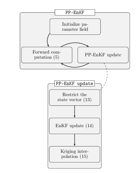
Figure 1: Diagram of the PP-EnKF workflow. The numbers point to the equation of the corresponding step.

To define the update of the PP-KF, the state vector and its covariance matrix are split into three parts, the pilot point parameters, the non-pilot point parameters, and the dynamic variables. In order to introduce notation and make clear which part of the state vector is left out in the PP-KF, we now rewrite the full state vector and covariance matrix:

$$\mathbf{x}^{f}=\begin{pmatrix}\mathbf{x}^{f}_{p}\\ \mathbf{x}^{f}_{r}\\ \mathbf{x}^{f}_{d}\end{pmatrix}\in R^{n_{s}}\qquad\mathbf{P}=\begin{pmatrix}\mathbf{P}_{pp}&\mathbf{P}_{pr}&\mathbf{P}_{pd}\\ \mathbf{P}_{rp}&\mathbf{P}_{rr}&\mathbf{P}_{rd}\\ \mathbf{P}_{dp}&\mathbf{P}_{dr}&\mathbf{P}_{dd}\\ \end{pmatrix}\in R^{n_{s}\times n_{s}}\ .$$ (7)

Here, $\mathbf{x}^{f}_{p}\in R^{n_{p}}$ contains parameter values at pilot point positions, and $n_{p}$ is the number of pilot point parameters. $\mathbf{x}^{f}_{r}\in R^{n_{r}}$ denotes the parameters at non-pilot point locations, where $n_{r}$ is the number of non-pilot point parameters. Finally, $\mathbf{x}^{f}_{d}\in R^{n_{d}}$ contains the $n_{d}$ dynamic variables. The sum $n_{s}=n_{p}+n_{r}+n_{d}$ is the total number of entries in the state vector. The covariance matrix $\mathbf{P}_{pp}\in R^{n_{p}\times n_{p}}$ contains the covariances between all pairs of parameters at pilot points. $\mathbf{P}_{pr}\in R^{n_{p}\times n_{r}}$ and $\mathbf{P}_{rp}\in R^{n_{r}\times n_{p}}$ contain covariances between parameters at pilot points and parameters at non-pilot points. $\mathbf{P}_{rr}\in R^{n_{r}\times n_{r}}$ contains covariances between pairs of parameters at non-pilot points. $\mathbf{P}_{dp}\in R^{n_{d}\times n_{p}}$ and $\mathbf{P}_{pd}\in R^{n_{p}\times n_{d}}$ contain covariances between dynamic variables and parameters at pilot points. $\mathbf{P}_{dr}\in R^{n_{d}\times n_{r}}$ and $\mathbf{P}_{rd}\in R^{n_{r}\times n_{d}}$ contain covariances between dynamic variables and parameters at non-pilot points. Finally, $\mathbf{P}_{dd}\in R^{n_{d}\times n_{d}}$ contains covariances between pairs of dynamic variables.

The update of the PP-KF consists of two steps: updating the parameters at pilot points and then interpolating the update. First, the pilot point update equations are discussed. The form of the mean vector update equation is identical to Equation (3) of the Kalman filter, restricted to dynamic variables and pilot-point parameters:

$$\begin{pmatrix}\mathbf{x}^{a}_{p}\\ \mathbf{x}^{a}_{d}\end{pmatrix}-\begin{pmatrix}\mathbf{x}^{f}_{p}\\ \mathbf{x}^{f}_{d}\end{pmatrix}=\begin{pmatrix}\mathbf{P}_{pp}&\mathbf{P}_{pd}\\ \mathbf{P}_{dp}&\mathbf{P}_{dd}\end{pmatrix}\mathbf{H}^{T}\left(\mathbf{P}_{yppy}+\mathbf{R}\right)^{-1}\left(\mathbf{d}-\mathbf{H}\begin{pmatrix}\mathbf{x}^{f}_{p}\\ \mathbf{x}^{f}_{d}\end{pmatrix}\right)\ .$$ (8)

Explanations for the PP-KF versions of the covariance matrix among simulated measurements $\mathbf{P}_{yppy}\in R^{n_{m}\times n_{m}}$ and the measurement operator $\mathbf{H}\in R^{n_{m}\times(n_{p}+n_{d})}$ can be found in Section 2.3.

The PP-KF update of the covariance matrix has the same form as Equation (4), but again restricted to dynamic variables and parameters at pilot points:

$$\begin{pmatrix}\mathbf{P}^{a}_{pp}&\mathbf{P}^{a}_{pd}\\ \mathbf{P}^{a}_{dp}&\mathbf{P}^{a}_{dd}\end{pmatrix}-\begin{pmatrix}\mathbf{P}_{pp}&\mathbf{P}_{pd}\\ \mathbf{P}_{dp}&\mathbf{P}_{dd}\end{pmatrix}=-\begin{pmatrix}\mathbf{P}_{pp}&\mathbf{P}_{pd}\\ \mathbf{P}_{dp}&\mathbf{P}_{dd}\end{pmatrix}\mathbf{H}^{T}\left(\mathbf{P}_{yppy}+\mathbf{R}\right)^{-1}\mathbf{H}\begin{pmatrix}\mathbf{P}_{pp}&\mathbf{P}_{pd}\\ \mathbf{P}_{dp}&\mathbf{P}_{dd}\end{pmatrix}\ .$$ (9)

$\mathbf{x}^{a}_{p}$ and $\mathbf{P}^{a}_{pp}$ are the updates of mean vector and covariance matrix of the parameters at pilot point locations, $\mathbf{x}^{a}_{d}$ and $\mathbf{P}^{a}_{dd}$ are the corresponding quantities for the dynamic variables. $\mathbf{P}^{a}_{dp}$ and $\mathbf{P}^{a}_{pd}$ contain updated covariances between pilot-point parameters and dynamic variables.

Now we discuss the second step, i.e., the transfer of the update to non-pilot point parameters by kriging interpolation. Through the kriging interpolation, the updates from Equations (8) and (9) are used to compute updates for means and covariances of parameters at non-pilot points:

$$\mathbf{x}^{a}-\mathbf{x}^{f}\ =P_{p}\left[\begin{pmatrix}\mathbf{x}^{a}_{p}\\ \mathbf{x}^{a}_{d}\end{pmatrix}-\begin{pmatrix}\mathbf{x}^{f}_{p}\\ \mathbf{x}^{f}_{d}\end{pmatrix}\right]$$ (10)

The interpolation operator $P_{p}$ is defined as

$$P_{p}=\begin{pmatrix}1&0\\ \mathbf{P}_{rp}^{0}\mathbf{P}_{pp}^{-1}&0\\ 0&1\\ \end{pmatrix}\in R^{n_{s}\times(n_{p}+n_{d})}\ .$$ (11)

Here, $\mathbf{P}_{rp}^{0}\in R^{n_{r}\times n_{p}}$ is a fixed covariance matrix between pilot point parameters and non-pilot point parameters. The matrix $\mathbf{P}_{rp}^{0}$ is specified in advance. A suitable choice for $\mathbf{P}_{rp}^{0}$ are prior covariances equal to the covariances used in the generation of the prior parameter fields as these covariances reflect the prior knowledge. The interpolation equation for the covariance matrix is

$$\mathbf{P}^{a}-\mathbf{P}=P_{p}\left[\begin{pmatrix}\mathbf{P}^{a}_{pp}&\mathbf{P}^{a}_{pd}\\ \mathbf{P}^{a}_{dp}&\mathbf{P}^{a}_{dd}\end{pmatrix}-\begin{pmatrix}\mathbf{P}_{pp}&\mathbf{P}_{pd}\\ \mathbf{P}_{dp}&\mathbf{P}_{dd}\end{pmatrix}\right]P_{p}^{T}\ .$$ (12)

A closer discussion of the interpolation operator $P_{p}$ can be found in Section 2.3.

The equations for the PP-EnKF are very similar to Equations (7), (8), and (10) for the mean update of the PP-KF. The state vector is split for every realization in the ensemble:

$$\mathbf{x}^{f}_{i}=\begin{pmatrix}\mathbf{x}^{f}_{p,i}\\ \mathbf{x}^{f}_{r,i}\\ \mathbf{x}^{f}_{d,i}\end{pmatrix}\in R^{n_{s}}\ ,\qquad i\in\left\{1,\cdots,n_{e}\right\}\ .$$ (13)

Then, the update of the state vector is calculated for each realization of pilot point parameters and dynamic variables:

$$\begin{pmatrix}\mathbf{x}^{a}_{p,i}\\ \mathbf{x}^{a}_{d,i}\end{pmatrix}-\begin{pmatrix}\mathbf{x}^{f}_{p,i}\\ \mathbf{x}^{f}_{d,i}\end{pmatrix}=\begin{pmatrix}\mathbf{P}_{pp,e}&\mathbf{P}_{pd,e}\\ \mathbf{P}_{dp,e}&\mathbf{P}_{dd,e}\end{pmatrix}\mathbf{H}^{T}\left(\mathbf{P}_{yppy,e}+\mathbf{R}\right)^{-1}\left(\mathbf{d}_{i}-\mathbf{H}\begin{pmatrix}\mathbf{x}^{f}_{p,i}\\ \mathbf{x}^{f}_{d,i}\end{pmatrix}\right),\qquad i\in\left\{1,\cdots,n_{e}\right\}.$$ (14)

Finally, the interpolation is applied to each realization:

$$\mathbf{x}^{a}_{i}-\mathbf{x}^{f}_{i}\ =P_{p}\left(\begin{pmatrix}\mathbf{x}^{a}_{p,i}\\ \mathbf{x}^{a}_{d,i}\end{pmatrix}-\begin{pmatrix}\mathbf{x}^{f}_{p,i}\\ \mathbf{x}^{f}_{d,i}\end{pmatrix}\right)\ ,\qquad i\in\left\{1,\cdots,n_{e}\right\}.$$ (15)

There are two main differences between the updates of the PP-EnKF and the PP-KF. First, the update of the PP-EnKF consists of $n_{e}$ equations, one for each realization of the ensemble. Second, all covariance matrices except $\mathbf{P}_{rp}^{0}$ are calculated from the ensemble of state vector realizations. When moving from the PP-KF to the PP-EnKF, the initialization of the parameter field is randomized. Opposed to this randomization, the variability outside the pilot points, represented by the fixed matrix $\mathbf{P}_{rp}^{0}$, is chosen once and then fixed throughout the computation. In the next section, important matrices of the PP-KF and the PP-EnKF algorithms are explained in more detail.

2.3 Covariance matrix of the simulated observations and interpolation operator

The matrix $\mathbf{P}_{yppy}$ used in the update equations (8) and (9) of the PP-KF is an approximation of the covariance matrix of simulated measurement variables $\mathbf{P}_{yy}$ appearing in the Kalman update (Equation (3)):

$$\mathbf{P}_{yy}=\mathbf{H}\mathbf{P}\mathbf{H}^{T}$$ (16)

$\mathbf{P}_{yppy}$ should approximate $\mathbf{P}_{yy}$ by taking into account only the dynamic variables and the pilot point parameters. The straightforward approximation with this property is obtained by removing the covariances that contain information from the non-pilot point locations, i.e. $\mathbf{P}_{rp}$, $\mathbf{P}_{pr}$, $\mathbf{P}_{rr}$, $\mathbf{P}_{dr}$, and $\mathbf{P}_{rd}$, from $\mathbf{P}$ before applying $\mathbf{H}$.

$$\mathbf{P}_{yppy}=\mathbf{H}\begin{pmatrix}\mathbf{P}_{pp}&0&\mathbf{P}_{pd}\\ 0&0&0\\ \mathbf{P}_{dp}&0&\mathbf{P}_{dd}\\ \end{pmatrix}\mathbf{H}^{T}$$ (17)

Note that $\mathbf{P}_{yppy}=\mathbf{P}_{yy}$ if $\mathbf{H}$ is a linear operator depending only on pilot point parameters and dynamic variables. A simple example of such a measurement operator $\mathbf{H}$ arises when all measurement variables are either dynamic variables or parameters at pilot points. For the PP-EnKF, the above remains true, with the amendment that the covariance matrices $\mathbf{P}_{yppy,e},\mathbf{P}_{yy,e},\mathbf{P}_{pp,e},\mathbf{P}_{pd,e},\mathbf{P}_{dp,e}$, and $\mathbf{P}_{dd,e}$ are calculated from an ensemble of realizations.

Now the interpolation operator is discussed. The operator $P_{p}$ defines the kriging interpolation, the second part of the update of both the PP-KF and the PP-EnKF. It determines the updates of non-pilot point parameters based on the updates of pilot point parameters. The definition of $P_{p}$ was given in Equation (11), and it makes use of two covariance matrices, $\mathbf{P}_{pp}$ and $\mathbf{P}_{rp}^{0}$. The covariance matrix of the pilot point parameters $\mathbf{P}_{pp}$ is obtained from the forward simulation. Thus, the knowledge of $\mathbf{P}_{pp}$ originates from a mixture of the initially drawn prior covariance matrix and of the filter equations that were applied before the current update. In contrast, the covariance between the non-pilot point parameters and the pilot point parameters $\mathbf{P}_{rp}^{0}$ is fixed throughout the computation. The superscript zero emphasizes two characteristic features of $\mathbf{P}_{rp}^{0}$. First, $\mathbf{P}_{rp}^{0}$ is fixed and, second, its elements may be prior covariances. In our synthetic experiments, we construct the prior covariances $\mathbf{P}_{rp}^{0}$ from the initial permeability field ensemble. The initial permeability field ensemble itself is obtained by Sequential Gaussian Simulation using prior information in the form of a semivariogram (SGSIM, Deutsch and Journel (1992)). Fixing $\mathbf{P}_{rp}^{0}$ is an integral part of the PP-EnKF, because this fixed covariance is one of the two reasons why we expect the PP-EnKF to suppress spurious correlations between pilot point parameters and non-pilot point parameters, the other reason being the reduction of the number of parameters in the Kalman update.

2.4 Comparison to the classical EnKF and other EnKF methods

We compare the update equations (14) and (15) of the PP-EnKF to the update equation (6) of the classical EnKF. If the measurement operator $\mathbf{H}$ operates on parameters at non-pilot points, this particular measurement information will be lost through the approximation in the PP-EnKF update, as shown in section 2.3. This is a hypothetical case, because one can always locate pilot points at parameter measurement locations. If the measurement operator $\mathbf{H}$ operates only on parameters at pilot points and dynamic variables, the main difference between the update equations is the kriging interpolation of the PP-EnKF. $\mathbf{P}_{e}$ in the update equation (6) of the EnKF can be partitioned the same way as in Equation (7):

$$\mathbf{P}_{e}=\begin{pmatrix}\mathbf{P}_{pp,e}&\mathbf{P}_{pr,e}&\mathbf{P}_{pd,e}\\ \mathbf{P}_{rp,e}&\mathbf{P}_{rr,e}&\mathbf{P}_{rd,e}\\ \mathbf{P}_{dp,e}&\mathbf{P}_{dr,e}&\mathbf{P}_{dd,e}\\ \end{pmatrix}\in R^{n_{s}\times n_{s}}.$$ (18)

The middle column of this matrix does not influence the update equation, if the aforementioned restrictions on $\mathbf{H}$ hold. In the PP-EnKF, $\mathbf{P}_{e}$ is approximated by

$$P_{p}\begin{pmatrix}\mathbf{P}_{pp,e}&\mathbf{P}_{pd,e}\\ \mathbf{P}_{dp,e}&\mathbf{P}_{dd,e}\end{pmatrix}=\begin{pmatrix}1&0\\ \mathbf{P}_{rp}^{0}\mathbf{P}_{pp,e}^{-1}&0\\ 0&1\\ \end{pmatrix}\begin{pmatrix}\mathbf{P}_{pp,e}&\mathbf{P}_{pd,e}\\ \mathbf{P}_{dp,e}&\mathbf{P}_{dd,e}\end{pmatrix}=\begin{pmatrix}\mathbf{P}_{pp,e}&\mathbf{P}_{pd,e}\\ \color[rgb]{1,0,0}{\mathbf{P}_{rp}^{0}}&\color[rgb]{1,0,0}{\mathbf{P}_{rp}^{0}\mathbf{P}_{pp,e}^{-1}\mathbf{P}_{pd,e}}\\ \mathbf{P}_{dp,e}&\mathbf{P}_{dd,e}\\ \end{pmatrix}\,.$$ (19)

It is of interest to compare the two columns of matrix (19) to the first and last column of $\mathbf{P}_{e}$ in Equation (18). Differences between the two matrices appear in the second row. The left columns of these matrices determine the update coming from measurements of parameters at pilot points. The updates of the EnKF and the PP-EnKF would be equal if the fixed covariance matrix $\mathbf{P}_{rp}^{0}$ were equal to the ensemble covariance $\mathbf{P}_{rp,e}$ from the EnKF. Of course, the matrices will never be exactly equal due to sampling fluctuations. One of the positive effects of $\mathbf{P}_{rp}^{0}$ is that it does not suffer from spurious correlations.

The right column of matrix (19) determines the update coming from measurements of dynamic variables. Values at non-pilot points are updated according to $\mathbf{P}_{rp}^{0}\mathbf{P}_{pp,e}^{-1}\mathbf{P}_{pd,e}$ instead of $\mathbf{P}_{rd,e}$. There is no direct covariance matrix between non-pilot points and dynamic variables in the PP-EnKF. Instead, the update is correlated with the pilot points and then interpolated according to $\mathbf{P}_{rp}^{0}$. Again, the main enhancement is the reduction of spurious correlations.

We now compare the update equations of the PP-EnKF to the update equations of two popular EnKF methods, the local EnKF and the hybrid EnKF. Similarly to the local EnKF and the hybrid EnKF, the PP-EnKF uses a partially fixed covariance structure in order to suppress spurious correlations. In the local EnKF, updates are calculated directly for all parameters, but correlations between parameters (or correlations between dynamic variables and parameters) are set to zero if their distance to measurement locations exceeds a certain threshold. Like the local EnKF, the PP-EnKF aims to suppress spurious correlations. To achieve this, only the correlations between measurement variables and pilot points are calculated from the ensemble. We argue that the PP-EnKF could be preferred to the local EnKF in cases, when distant locations are significantly correlated. Correlations between these locations would be suppressed by the local EnKF, while the PP-EnKF includes them through correlations between distant pilot point locations.

In the hybrid EnKF, a mixture of covariance matrices is used in the update step, partially fixed and partially calculated from the ensemble. While this can lead to good results, we argue that the PP-EnKF delivers an appealing alternative, because it interferes less with the statistics of the update step. The first step of the update of the PP-EnKF is restricted to pilot point parameters and dynamic variables. As a benefit, the update for these two sets of state vector variables is calculated exclusively from the ensemble-based correlations that are derived from the ensemble of forward model runs. Only the rest of the parameters is then updated by kriging the updates at the pilot points, using the pre-defined fixed covariance matrix. For the hybrid EnKF, all updates are, at least partially, subject to the pre-defined, fixed covariance matrix.

An additional benefit of the PP-EnKF is that its implementation is relatively straightforward. In contrast to the hybrid or the local EnKF, there is no need to change the covariance matrix of the classical EnKF update equation. All changes of the PP-EnKF (compared to the classical EnKF) can be implemented by pre-processing (restricting the state vector to dynamic variables and parameters at pilot points) and post-processing (calculating the interpolated parameter values at non-pilot points). Thus, a modular implementation around an existing implementation of the EnKF update is possible.

2.5 Optimality considerations for the PP-EnKF

Finally, in this section we discuss the optimality of the PP-EnKF. To this end, we consider the EnKF as the benchmark optimal method, even though it has its own limitations (Evensen, 2003). All filters in the comparisons described in this paragraph are considered to be applied in combination with an infinite ensemble, thus without any spurious correlations. For a given use case, two comparisons will be discussed between the PP-EnKF and two EnKF variants that will serve as optimality bounds (see also Table 1). The given use case can be thought of as the model setups described in this work, but the reasoning in this paragraph holds for any model setup where pilot points can be applied.

The first comparison is between the PP-EnKF and the EnKF, both applied in a synthetic data assimilation experiment for the given use case. By definition of its update, the PP-EnKF is sub-optimal to the EnKF for a given use case under perfect conditions, i.e., at the limit of infinite ensemble size. This is because the update of the PP-EnKF is interpolated while the update of the EnKF retains the full variability of the parameters in the state vector.

We now turn to the second comparison between the PP-EnKF and an altered EnKF, from now on called Interpolated EnKF. Again, both filters are applied in two synthetic data assimilation experiments for the same use case. The Interpolated EnKF uses a model setup that only consists of pilot point parameters and dynamic states. In the Interpolated EnKF, the full set of parameters is interpolated from the pilot points for both the updates and the forward computation. In our PP-EnKF, in contrast, the full set of parameters is used for the forward computation, while the updates are interpolated from the pilot points as in the Interpolated EnKF. It follows that the Interpolated EnKF is sub-optimal to the PP-EnKF, since it uses interpolated values in the forward computation, where the PP-EnKF retains the full variability of the (infinite and correct) initial parameter ensemble. On the other hand, the Interpolated EnKF is still optimal on its own right when defining the pilot points to be the only parametric degrees of freedom of the same use case.

In summary, the PP-EnKF is theoretically sub-optimal to the EnKF, while the Interpolated EnKF is sub-optimal to the PP-EnKF, although optimal under purely pilot point based parametrization. This way, we use the EnKF and the Interpolated EnKF as optimality bounds for the PP-EnKF. As a final remark, when realistic models and limited ensemble sizes are considered, the PP-EnKF regains its advantage over the EnKF regarding the suppression of spurious correlations that we illustrate in this study.

Table 1: Optimality bounds for the PP-EnKF. The PP-EnKF is compared to the EnKF and to the Interpolated EnKF that is defined in the text.

full variability in…	EnKF	PP-EnKF	Interpolated EnKF
forward computation	✓	✓	x
update equation	✓	x	x

3 Design of the synthetic experiments

The performance of the PP-EnKF is evaluated by comparing it to seven other EnKF methods (damped, iterative, local, hybrid, dual (Moradkhani et al., 2005), normal score (NS-EnKF Zhou et al., 2011, Schöniger et al., 2012, Li et al., 2012, Goovaerts, 1997, Journel and Huijbregts, 1978) and classical). The comparison procedure is adopted from Keller et al. (2018). As in (Keller et al., 2018), the performance evaluations are carried out for two parameter estimation setups: a 2D tracer transport problem and a 2D flow problem with one injection well. The estimated parameter field in these setups is the permeability field that largely determines the hydraulic conductivity field in the subsurface. In each setup, $1,000$ synthetic experiments are computed for the PP-EnKF and for the seven other EnKF methods, and each one for ensemble sizes of 50, 70, 100, and 250. In each experiment, we assess both the updated parameter fields and their ensemble variance. The ensemble variance is compared to a reference EnKF estimation with a very large ensemble size of 10,000. Next to the RMSE comparison, there is a comparison of the correlation fields driving the Kalman update using 10 synthetic experiments for ensemble size 50. The correlation output of these synthetic experiments is compared to the correlation field of the reference EnKF with ensemble size 10,000 by computing the RMSE difference of the correlation fields. Additionally, the impact of the correlation length of the prior permeability fields is investigated. The correlation length is important in the PP-EnKF, because it not only affects the prior permeability field but also the kriging interpolation. Finally, to check the influence of the pilot point grid on the performance of the PP-EnKF, different grid configurations are tested.

3.1 Subsurface models

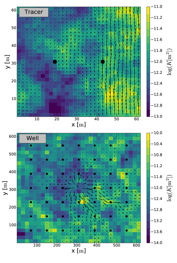
Figure 2: The logarithmic reference permeability fields for the tracer model and the well model with groundwater flow vectors. Measurement locations are depicted as black circles. Figure taken from Keller et al. (2018).

The performance comparison of the PP-EnKF with other EnKF-variants in this study is carried out for two transient subsurface model setups, first, a 2D solute transport model (tracer model), and, second, a 2D groundwater flow problem with an injection well and four pumping wells (well model). These model setups have already been used in a previous publication that compared existing EnKF methods without the PP-EnKF and are used as benchmark for the PP-EnKF here (Keller et al., 2018). The grids of both models consist of $31\times 31=961$ identical squared cells. The size of the model domain for the tracer model is $62\,\mathrm{m}\times 62\,\mathrm{m}$; the size of the model domain for the well model is $620\,\mathrm{m}\times 620\,\mathrm{m}$. The simulation period is $1,200$ days for the tracer model and $18$ days for the well model. For both models, the simulation period is divided into $1,200$ time steps. All forward simulations are computed with the numerical software SHEMAT-Suite (Rath et al., 2006, Clauser, 2012, Keller et al., 2020).

In the tracer model, a constant head difference of $11\,\mathrm{m}-10\,\mathrm{m}=1\,\mathrm{m}$ is implemented between the southern boundary and the northern boundary, accompanied by a constant concentration difference of $80\times 10^{-3}\,\mathrm{mol}/\mathrm{L}-60\times 10^{-3}\,\mathrm{mol}/\mathrm{L}=20\times 10^{-3}\,\mathrm{mol}/\mathrm{L}$. The remaining two boundaries are impermeable. The initial conditions are a head of $10\,\mathrm{m}$ and a concentration of $60\times 10^{-3}\,\mathrm{mol}/\mathrm{L}$ throughout the model domain for the tracer model. In the well model, a head difference of $1\,\mathrm{m}$ is implemented between a central injection well location at coordinates ($310\,\mathrm{m}$, $310\,\mathrm{m}$) and the four boundaries. Initial head is chosen as $10\,\mathrm{m}$ throughout the model domain for the well model. For both setups, standard properties of water are used and the porosity of the background matrix is $10\%$. The tracer is subjected to advective transport only.

Measurement locations vary between the two setups. The tracer model includes two measurement locations at coordinates $\left(19\,\mathrm{m},31\,\mathrm{m}\right)$ and $\left(43\,\mathrm{m},31\,\mathrm{m}\right)$. At these locations, tracer concentration and hydraulic head measurements are available at $100$ evenly distributed times throughout the simulation period. The well model includes 49 measurement locations on a $7\times 7$ grid throughout the model domain. At these locations, hydraulic head measurements are available at $60$ evenly distributed times throughout the simulation period.

The synthetic reference permeability distributions for the two subsurface model setups are displayed in Figure 2. These permeability fields are generated by sequential multi-Gaussian simulation (SGSIM, Deutsch and Journel (1992)). The same holds for the ensemble of prior permeability field realizations that is used to initialize the EnKF. A permeability mean of $-12.0\,\log_{10}(K[\mathrm{m}^{2}])$ is used for the synthetic reference and a permeability mean of $-12.5\,\log_{10}(K[\mathrm{m}^{2}])$ is used for the prior permeability distributions. In both cases, the standard deviation is $0.5\,\log_{10}(K[\mathrm{m}^{2}])$. The isotropic correlation length of the permeability fields is $50\,\mathrm{m}$ for the tracer model and $60\,\mathrm{m}$ for the well model. No nugget effect is used. More details on the spherical correlation function used can be found in Keller et al. (2018). Additionally, the input files for the sequential Gaussian simulation can be found in the data repository of this publication.

3.2 Parameter settings for the PP-EnKF and other EnKF variants

Measurement noises are equal for all EnKF methods including the PP-EnKF. Measurement noises for the concentration measurements of the tracer model are set to $\sigma_{\mathtt{c}}=7.1\times 10^{-3}\mathrm{mol}/\mathrm{L}$ and measurement noises for the hydraulic head measurements of both setups are set to $\sigma_{\mathtt{h}}=5\times 10^{-2}\leavevmode\nobreak\ \mathrm{m}$. EnKF methods which require parameter settings include the damped EnKF, where the damping constant is set to $0.1$ (Hendricks Franssen and Kinzelbach, 2008). In the local EnKF, the length scale (which is half the cutoff radius) is set to $150\,\mathrm{m}$, which is larger than the correlation lengths. In the hybrid EnKF, the mixing constant is set to $0.5$ and a diagonal background covariance matrix is specified. The damping factor of the damped EnKF and the parameter choices of the local EnKF and the hybrid EnKF were shown to yield the smallest root mean square errors in most synthetic experiments of the two setups of a previous performance comparison (Keller et al., 2018).

The PP-EnKF needs as inputs the locations for the pilot points, and a covariance matrix for the kriging interpolation. We use 51 pilot points including all cell indices of the measurement locations of both setups (tracer model and well model). Thus, the pilot points lie on a $7\times 7$ grid for both model setups with two additional pilot points in the center of the model corresponding to the measurement locations of the tracer model. A regular grid of pilot points is documented to be beneficial (Capilla et al., 1997). The interpolation covariance $\mathbf{P}^{0}_{rp}$ is chosen identical to the prior covariance. This is implemented by computing the covariances in $\mathbf{P}^{0}_{rp}$ from 10,000 permeability fields, which are generated by SGSim with the same correlation length, mean and standard deviation as the prior permeability fields.

3.3 Performance Comparison Setup

In Keller et al. (2018), seven EnKF variants have been compared (damped, iterative, local, hybrid, dual, normal score and classical). Now, we compare the PP-EnKF to these same seven methods by computing synthetic experiments for the two physical model setups introduced in the previous sections (compare Section 4.1). Additionally, correlation lengths of the initial permeability fields of both setups are varied to half and twice the correlation length of the synthetic truth (Section 4.3). This is done, because the correlation length plays a very prominent role in the PP-EnKF, more prominent than in the other EnKF methods, since it enters in the PP-EnKF not only as correlation length of the prior permeability field, but also as correlation length of the kriging interpolation. Thus, it is especially important to see how the PP-EnKF performs compared to other models, when it is subject to mis-specified correlation lengths. One important degree of freedom in the PP-EnKF is the choice of the grid of pilot points. Thus, we compare the results of different sensible grid choices for the two model setups (Section 4.5). Next to the performance of the mean update, we are interested in the spatial variability of the permeability ensemble update by the PP-EnKF. This will help assess the ability of the PP-EnKF to suppress spurious correlations. To evaluate the reproduction of the uncertainty of the estimates, we compare the overall standard deviation of the ensembles generated by the updates of the various EnKF methods. For each EnKF method, 1,000 synthetic experiments are used. The synthetic experiments differ solely in their random seed for geostatistical ensemble initialization and measurement perturbation. Additionally, the full correlation fields of the EnKF and the PP-EnKF from 10 synthetic experiments are compared to a reference correlation field.

3.4 Performance Comparison Measures

Multiple synthetic experiments are needed to compare EnKF methods (Keller et al., 2018). Here we use root-mean-square errors (RMSEs) from 1,000 synthetic experiments to compare the PP-EnKF to the other seven EnKF methods. For each synthetic experiment $j$, the RMSE is computed as follows

$$\mathrm{RMSE}_{j}=\sqrt{\frac{1}{n_{g}}\sum_{i=1}^{n_{g}}\left(\bar{Y}_{i,j}-Y^{t}_{i,j}\right)^{2}},\qquad j\in\left\{1,\cdots,1000\right\}.$$ (20)

Such a single RMSE is computed from the squared differences of estimated mean logarithmic permeabilities $\bar{\mathbf{Y}}_{j}\in R^{n_{g}}$ and the synthetic reference $\mathbf{Y}^{t}_{j}\in R^{n_{g}}$ across the $n_{g}$ grid cells.

The RMSE measures the distance between the average over the estimated permeability field realizations and the synthetic true permeability field. Additionally, the overall standard deviation among realizations is introduced as a measure for the uncertainty of the estimated permeability field realizations. It is called STD in the remainder of this text. This overall standard deviation for a single synthetic experiment $j$ is calculated as the square root of the mean over the domain of the pixel-wise ensemble variances, as follows

$$\mathrm{STD}_{j}=\sqrt{\frac{1}{n_{g}}\sum_{i=1}^{n_{g}}\sigma_{i,j}^{2}},\qquad j\in\left\{1,\cdots,1000\right\}.$$ (21)

where $n_{g}$ is the number of grid cells. The sample variances in Equation (21) are calculated as follows

$$\sigma_{i,j}^{2}=\frac{1}{n_{e}-1}\sum_{k=1}^{n_{e}}\left(Y_{k,i,j}-\bar{Y}_{i,j}\right)^{2}$$ (22)

where $n_{e}$ is the number of realizations in the ensemble, $\bar{Y}_{i,j}$ is the mean logarithmic permeability for synthetic experiment $j$ and grid cell $i$, and $Y_{k,i,j}$ is the permeability of realization $k$ calculated at grid cell $i$ in synthetic experiment $j$.

Besides the overall performance assessment combining results of the RMSE and STD, a smaller test with 10 synthetic experiments is carried out for checking the correlations between observed variables and the full parameter field. This input/output-intensive check is executed only for the PP-EnKF and the classical EnKF. A reference synthetic experiment is computed using the EnKF with an ensemble size of 10,000. Subsequently, 10 synthetic experiments were computed for EnKF and PP-EnKF using ensemble size 50. For the tracer model, the correlations are of the form

$$\rho(c_{obs},K)=\frac{\mathrm{Cov}(c_{obs},K)}{\sigma_{c}\cdot\sigma_{K}}$$ (23)

where the covariance $\mathrm{Cov}$ and the standard deviations $\sigma$ are estimated from the ensemble, $c_{obs}$ denotes the concentration at one of the two observation locations, and $K$ denotes the logarithmic permeability at any given location in the field. For the well model, the correlations are of the form

$$\rho(h_{obs},K)=\frac{\mathrm{Cov}(h_{obs},K)}{\sigma_{h}\cdot\sigma_{K}}$$ (24)

where the difference to the tracer case is that $h_{obs}$ denotes the head observed at one of the 49 measurement locations. By varying $K$ across the model domain, we obtain the field of correlations for each synthetic experiment. The RMSEs between these correlation fields and the reference correlation field is used to judge the amount of spurious correlation in the synthetic experiments introduced by the small ensemble size.

4 Results

4.1 Comparison of the PP-EnKF to other EnKF methods

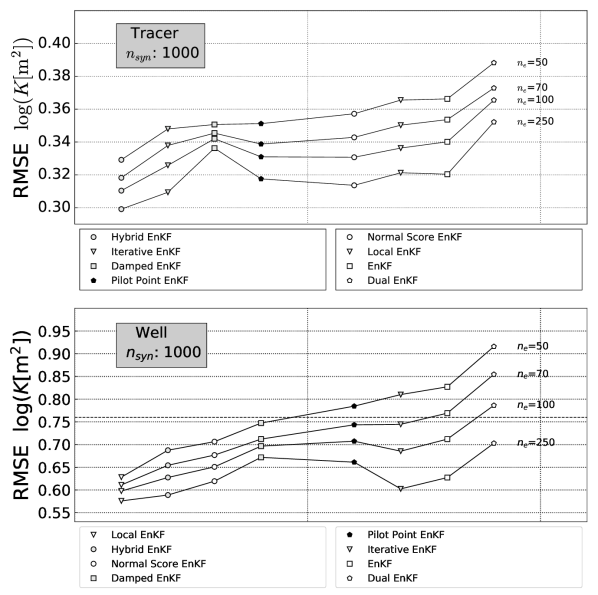
Figure 3: Comparison of the root mean square errors (RMSEs) of the pilot point EnKF and other EnKF methods in the tracer model (top) and well model (bottom).

To assess its performance, we compare the PP-EnKF to seven other EnKF methods. First, results for the tracer model setup are shown. In Figure 3 (top), the mean RMSEs from 1,000 synthetic experiments are shown for the eight EnKF methods. Numerical results are given in the supporting information. The tracer model is known to yield a small range of RMSEs across the tested EnKF methods (Keller et al., 2018). Among the eight tested EnKF methods, the PP-EnKF ranks among the four methods with the smallest RMSEs for all tested ensemble sizes. For ensemble size 50 and 250, the PP-EnKF has the fourth smallest RMSE. For ensemble sizes 70 and 100, it yields the third smallest RMSE.

A direct comparison to the classical EnKF is interesting for two reasons. First, the PP-EnKF is directly derived from the classical EnKF. Second, earlier publications include conflicting results regarding this comparison. In the synthetic experiments performed with our tracer model, the PP-EnKF performs significantly better than the classical EnKF for ensemble sizes 50 70, and 100, and slightly better for ensemble size 250.

Turning to results from the well model setup, Figure 3 (bottom) shows the RMSE means from the corresponding 1,000 synthetic experiments. Numerical results are given in the supporting information. Compared to the tracer model, the well model yields larger RMSE differences between the tested methods. The PP-EnKF yields slightly worse than average RMSEs for the well model. For ensemble size 50 and 70, the PP-EnKF has the fifth smallest RMSE. For ensemble sizes 100, and 250, it scores the sixth smallest RMSE. Compared to the classical EnKF, the PP-EnKF performs better for ensemble sizes 50, 70, slightly better for ensemble size 100, and worse for ensemble size 250.

Summing up the results for the two physical model setups, the PP-EnKF yields good RMSE results for the tracer model and medium RMSE results for the well model. It should be noted that these setups were taken from our previous study, and that a very robust testing was done using $1,000$ synthetic studies. Results from both physical model setups suggest that, for small ensemble sizes, the PP-EnKF is a clear improvement to the classical EnKF as desired by design. This is in slight contradiction to results from Heidari et al. (2013), where the PP-EnKF yields larger RMSEs than the classical EnKF for a synthetic experiment with ensemble size 50. Our results for ensemble size 250, for which both methods yield similar results, are in agreement with similar results from Tavakoli et al. (2013).

Furthermore, the RMSEs suggest that the PP-EnKF provides a trade-off between damping and the normal EnKF. For ensemble size 50, the PP-EnKF has similar or larger RMSE than the damped EnKF, but smaller RMSE than the classical EnKF. Moving to larger ensemble sizes, the reduction of RMSE by the PP-EnKF is much larger than the reduction of RMSE by the damped EnKF. A possible explanation for this effect is that the interpolated updates of the PP-EnKF reduce spurious correlations and thereby reduce the number of divergent synthetic experiments for small ensemble sizes. For larger ensemble sizes, the relatively large reductions of the RMSEs of the PP-EnKF suggest that the interpolated updates of the PP-EnKF can incorporate more information than the damped updates of the damped EnKF.

The full RMSE distributions give a more in-depth picture of the performance of the EnKF methods. They are provided in the supporting information. The distributions illustrate how the RMSE means in the previous section were obtained. For the well model, one can see that the PP-EnKF yields a somewhat wider RMSE distribution than other methods.

4.2 Ensemble variance of conditional realizations

Now, we test and compare the uncertainty characterization of conditional realizations obtained from the PP-EnKF by looking at the overall ensemble standard deviations. The equations for the overall standard deviations were introduced in Section 3.4. We compare the mean overall standard deviations calculated over 1,000 synthetic experiments for each EnKF method. Additionally, a benchmark STD is derived from 100 synthetic experiments using the classical EnKF with ensemble size 10,000.

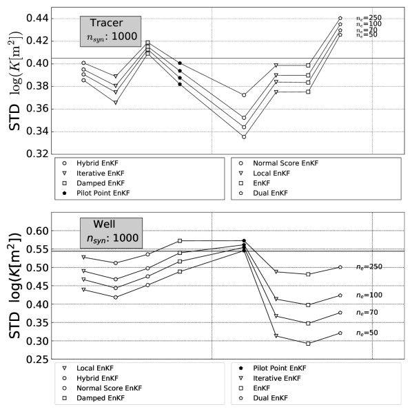
Figure 4: Comparison of the overall standard deviation (STD) of the pilot point EnKF and other EnKF variants for the tracer model (top) and well model (bottom). The horizontal black line depicts the STD obtained from 100 synthetic experiments with 10,000 ensemble members.

The results for the tracer model are shown in the top half of Figure 4. All EnKF methods yield standard deviations that are reasonably close to the standard deviation of the benchmark run. Still, most methods underestimate the ensemble spread; exceptions are the damped EnKF and the dual EnKF. Comparing the differences to the 10,000 ensemble run, the pilot point EnKF ranks fourth for ensemble size 50, third for ensemble sizes 70 and 100, and second for ensemble size 250. Thus, the pilot point EnKF is in the top half of the methods, not only for RMSE comparison, but also concerning the standard deviation.

For the well model, the mean overall standard deviations are shown in the bottom half of Figure 4. Compared to the tracer model, there is a larger tendency of most methods to underestimate ensemble spread compared to the 10,000 ensemble run. Additionally, one can see a clear difference between the EnKF methods that contain a form of damping and the ones that do not (including the iterative, classical and dual EnKF). The pilot point EnKF yields a large ensemble spread, especially for ensemble size 50, where it yields the best STD of all methods. For ensemble size 70, the pilot point EnKF still ranks first, for ensemble size 100 it ranks second and for ensemble size 250 it ranks third. Thus, while the pilot point EnKF only obtained medium results in RMSE comparison compared to other EnKF methods, it always ranks in the top three methods concerning uncertainty characterization, ranking first for the important smallest ensemble sizes.

In conclusion, the uncertainty characterization of the pilot point EnKF is generally good compared to other EnKF methods for the tracer model and well model. This is one of the main features of the method, and this benefit again comes by design. In the update step, the erroneous reduction of ensemble variance is constrained by two effects. First, by reducing the number of parameters to the number of parameters at pilot points, issues of rank deficiency and inbreeding are reduced, and second, by interpolating the update, large parts of the prior variability remain intact. Our results agree with results from Heidari et al. (2013), where a large spatial variability in PP-EnKF updates is diagnosed. While Tavakoli et al. (2013) also diagnose heterogeneities in the PP-EnKF results, the small ensemble spread in their PP-EnKF results is contradictory to our findings. This might be due to the specific subsurface model in (Tavakoli et al., 2013), where only a small fraction of the model parameters was updated.

4.3 Variation of prior correlation lengths

In this section, results for erroneous correlation lengths are discussed: the prior correlation lengths are varied to half or twice the correlation length of the synthetic truth. These results are especially important for judging the performance of the PP-EnKF, since it is influenced by the correlation length through both the prior realizations and the interpolation. The numerical RMSE results discussed in this section can be found in the supporting information.

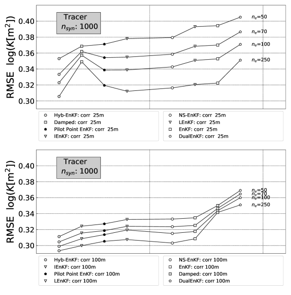
Figure 5: Comparison of the pilot point EnKF with other EnKF variants for the tracer model and correlation lengths $25\,\mathrm{m}$ (top) and $100\,\mathrm{m}$ (bottom).

First, we discuss the tracer model with correlation length $25\,\mathrm{m}$. This correlation length is half the correlation length of the synthetic truth. Figure 5 (top) shows the average RMSE values comparing to the results in Section 4.1. For ensemble size 50, all EnKF methods yield larger RMSEs than for the standard case. For ensemble size 250, all methods except the classical EnKF and the dual EnKF yield larger RMSEs than for the standard case. A specific look at the PP-EnKF shows that, for ensemble size 50, it ranks third among the EnKF methods. For ensemble sizes 70 and 100, it ranks second, and for ensemble size 250, third. Relatively to the other EnKF methods, these results are a slight improvement for the PP-EnKF compared to the case of the correct correlation length. This means that the PP-EnKF seems to be robust against a too small specification of correlation length for this test case.

Now we discuss the results for the tracer model and a too long correlation length of $100\,\mathrm{m}$ as shown in Figure 5 (bottom). For all ensemble sizes, all methods except the damped EnKF yield smaller RMSEs than for the correct correlation length ($50\,\mathrm{m}$). The damped EnKF yields slightly larger RMSEs for ensemble sizes 100 and 250 than for the standard case. Regarding the PP-EnKF, it ranks third among all methods for ensemble sizes 50, 70 and 100. For ensemble size 250, it ranks fourth among all methods. Thus, the ranking of the PP-EnKF among the different methods is comparable to the corresponding results for the correct correlation length.

For a discussion of these results, recall how an erroneous correlation length may affect the performance of EnKF methods. The correlation length primarily affects the prior permeability fields. This should generally be a disadvantage for the update, thus leading to larger RMSEs. An additional effect of the correlation length is its direct influence on the EnKF update. The correlations that drive the update are either more restricted to the vicinity of the measurement locations, for the case of a small correlation length, or they are spread out more widely for the case of the large correlation length. The RMSE result for the small correlation length suggest that the restriction of the EnKF update is particularly obstructive for the tracer model, possibly because there are only two measurement locations in this setup. Thus, for a small number of measurement locations, an underestimation of the correlation length may significantly inhibit EnKF updates. On the other hand, the smaller RMSEs for correlation length $100\,\mathrm{m}$ are surprising. This result suggests that the effect of the larger update radius is stronger than the effect of the wrong prior correlation length in the tracer setup. Good results for too large correlation lengths have been documented in the literature, for example by Chaudhuri et al. (2018). Chaudhuri et al. (2018) attribute this effect to two possible factors. First, too small correlation lengths may not capture the full information content of the observations, and second, the too long correlations lengths may lead to smoothed fields that prevent the appearance of locally strong deviations from the true reference field. However, the beneficial effect of long correlations lengths may vanish for more complicated synthetic reference fields, especially, when they exhibit small-scale heterogeneities. For example, in Camporese et al. (2011, 2015) it was found that an overestimated prior correlation length can propagate spurious correlations, leading to worse results than an underestimated prior correlation length.

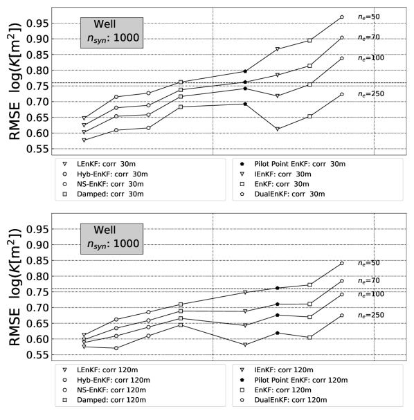
Figure 6: Comparison of the pilot point EnKF with other EnKF variants for the well model and correlation lengths $30\,\mathrm{m}$ (top) and $120\,\mathrm{m}$ (bottom).

Turning to the well model, the PP-EnKF for correlation length $30\,\mathrm{m}$ is tested. Figure 6 (top) shows RMSEs calculated over 1,000 synthetic experiments. Again, for all ensemble sizes, all EnKF methods yield slightly larger RMSEs than for the case of the correct correlation length ($60\,\mathrm{m}$). The PP-EnKF ranks fifth among the EnKF methods for ensemble sizes 50 and 70. For ensemble size 70 it ranks sixth and for ensemble size 250 seventh. This almost reproduces the results for the correct correlation length, only for ensemble size 250 the rank is slightly worse.

We now look at results for the well model and correlation length $120\,\mathrm{m}$ in Figure 6 (bottom). Here, for all ensemble sizes, all EnKF methods yield slightly smaller RMSEs than for the standard case. Regarding the PP-EnKF, it ranks sixth for ensemble sizes 50, 70 and 250, and it ranks seventh for ensemble size 100. Thus, again the ranking of the PP-EnKF among the methods is slightly worse than for the correct correlation length.

In summary, the PP-EnKF is not affected more by a mis-specification of the correlation length than other EnKF variants for both model setups, even though the correlation length has a more pronounced role in the PP-EnKF than in other variants. It has to be noted that the estimates the PP-EnKF may suffer from inaccuracy caused by inaccurate prior covariance matrices. In the synthetic experiments of this study, we estimate the effect on the PP-EnKF by deliberately choosing a slightly wrong initial mean of permeability fields, as well as, in this section, wrong correlation lengths in the construction of the correlation fields. Results for the PP-EnKF in these synthetic experiments are promising and do not show a worsening compared to other EnKF variants. However, especially in realistic, large-scale model setups, the issue of mis-specified correlations can arise for all EnKF variants and possibly with additional severity.

4.4 Average rankings of the PP-EnKF

In the last sections, various types of synthetic experiments were used to compare the performance of the PP-EnKF to other EnKF methods. This included synthetic experiments with the correct and erroneous prior correlation lengths, and repetitions for ensemble sizes of 50, 70, 100 and 250. In Table 2, the average RMSE rankings are displayed that are calculated from the twelve single RMSE rankings (four ensemble sizes for each of three correlation lengths). For the tracer setup, the PP-EnKF has the third best average ranking. Thus, for the tracer setup, the PP-EnKF has very good average results outperformed only by the hybrid EnKF and the iterative EnKF. For this setup, the performance of the PP-EnKF justifies its usage over the majority of other EnKF methods. For the well setup, the PP-EnKF only has the sixth best average ranking. For this setup, looking at the average RMSE would not justify using the PP-EnKF compared to existing EnKF variants.

Table 2: Average RMSE rankings of the eight EnKF methods for tracer and well setups. The average ranking is the mean of the twelve rankings from the RMSE comparisons of all tested prior correlation lengths.

RMSE	Tracer	Well
EnKF	6.1667	6.3333
Damped	5.9167	4.9167
NS-EnKF	3.9167	3.3333
DualEnKF	8.0	8.0
Hyb-EnKF	1.0	1.9167
LEnKF	5.4167	1.0833
IEnKF	2.3333	4.5833
PP-EnKF	3.25	5.833

Table 3: Average STD rankings of the eight EnKF methods for the tracer and well setups. The average ranking is the mean of the four rankings from the overall STD comparison.

STD	Tracer	Well
EnKF	4.75	8.0
Damped	2.25	2.0
NS-EnKF	7.75	2.5
DualEnKF	6.0	6.0
Hyb-EnKF	1.5	5.0
LEnKF	4.25	3.5
IEnKF	6.5	7.0
PP-EnKF	3.0	2.0

The reproduction of the correct ensemble variance is another key performance for comparing the EnKF methods. Therefore, overall STD results for the four ensemble sizes 50, 70, 100, 250 were ranked and subsequently averaged, and results are summarized in Table 3. The PP-EnKF performs well among the eight tested methods. For the tracer setup, the PP-EnKF ranks third out of eight methods. In particular, the PP-EnKF ranks significantly better than the iterative EnKF that ranked better for average RMSE. Thus, taking into account both, average RMSE and average STD, the PP-EnKF is outperformed only by the hybrid EnKF. For the well setup, the PP-EnKF ranks first together with damped EnKF. For the well setup and for small ensemble sizes, the PP-EnKF ranks undivided first.

4.5 Variation of pilot point grids

One important degree of freedom added by the PP-EnKF is the choice of the pilot points. In this section, RMSEs for different pilot point grids are compared in the tracer and well model.

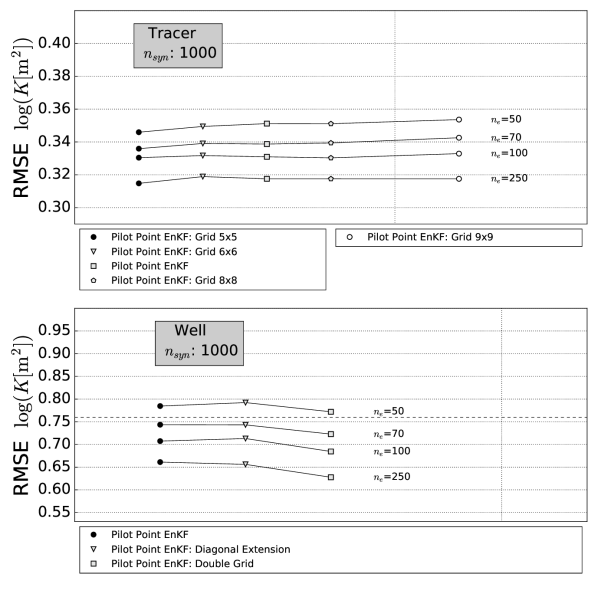
Figure 7: Mean RMSE (calculated over $1,000$ synthetic experiments) for PP-EnKF with different regular grids for the tracer setup (top) and well setup (bottom).

For the tracer model, the compared grids are regular square grids with different numbers of pilot points. All grids also include the two measurement locations of the tracer model. The results in Figure 7 (top) show small changes of the RMSE for different grids, all changes are smaller than $0.01\,\log_{10}(K[\mathrm{m}^{2}])$.

For the well model, the compared grids are extensions of the standard grid, since the standard grid is made up of all measurement locations. The first extension is adding pilot points on the diagonal between the original pilot points. The second extension is another regular grid with double the number of pilot points in each column and row. Again, the results in Figure 7 (bottom) exhibit small changes of the RMSE, only the doubled grid yields significantly smaller RMSE than the standard method.

The results of the grid variation suggest two implications. First, the differences between the grids are not very large, thus at least in the two setups treated here, the PP-EnKF shows a certain robustness against different choices of regular grids in the investigated range. Second, the results do also point in the direction that a smart choice of grid might make a bigger difference in other setups. While the grid with the smallest number of pilot points yields the smallest RMSEs for the relatively homogeneous synthetic true permeability field of the tracer model, the grid with the largest number of pilot points yields the smallest RMSEs for the more heterogeneous well model. This suggests a model-specific number of pilot points required to sufficiently approximate the real cross correlation functions. As a generic rule, we refer to the recommendations for pilot point spacing in the literature that suggest about three pilot points per range as a robust choice (Capilla et al., 1997). The range from Capilla et al. (1997) would correspond to two correlation lengths in our study, a distance at which parameters are barely correlated.

In this study, we discussed the most straightforward placing of pilot points on a regular grid. This pilot point placing is well adapted to this heterogeneous model setup (Hendricks Franssen, 2001, Doherty et al., 2010). Additionally, there are ways to optimize the placing of pilot points in the framework of optimal experimental design (Mehne et al., 2011) or using prior information (Alcolea et al., 2006). This could be adapted to the PP-EnKF by optimally placing pilot points. Options include measures derived from the sample covariance, and the pilot point locations could even be dynamically adapted during the assimilation, for example after each updating step. In future research, it would be interesting to check the influence of sophisticated pilot point placing methods on the performance of the PP-EnKF, especially in larger, more realistic model setups than discussed in this work. In summary, strategies to optimize the placing of pilot points are documented in the literature. However, this was beyond the scope of this work and requires substantial additional compute time. We followed here standard rules for placing of pilot points which gave the documented satisfactory results and were not subject to large changes in case of modifying the density of the pilot points. However, by optimizing the placing of the pilot points further performance gain might be achieved.

4.6 Spurious correlation reduction

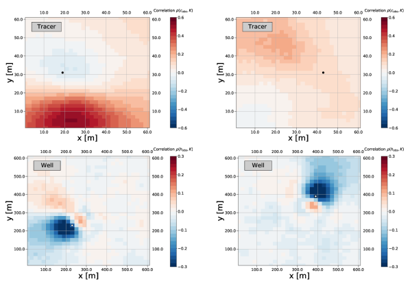
Figure 8: Reference correlations between an observed variable at a chosen observation location and the permeability throughout the model domain. For the tracer setup (top), the two observation locations for concentration are plotted in black, for the well setup (bottom) the two (out of 49) observation points for head are plotted in white.

Now the ability of the PP-EnKF to reduce spurious correlations is tested by checking the correlations between observed variables and updated permeabilities in the tracer and well setup after assimilation. As a benchmark, we use a reference synthetic experiment with the EnKF and 10,000 ensemble members. Figure 8 shows the reference correlation fields for the tracer and well setup after the EnKF updates. For the tracer setup, both observation locations are shown. The concentrations at the observation location in the highly permeable region (observation location on the right, compare the synthetic true permeability fields from Figure 2) yields comparably small correlations. The observation location in the low-permeable region (observation location on the left) yields large positive correlation with the low-permeability region south of the observation location. For the EnKF update, this positive correlation implies that larger measured tracer concentrations will lead to updates towards larger permeability values (promoting tracer transport towards the measurement location). Turning to the well setup, two representative head observation locations are displayed. One can observe a general trend, small positive correlations in the direction of the injection well in the center of the model and large negative correlations in the direction of the model boundaries. For the EnKF update, this means that higher measured hydraulic heads (smaller drawdowns) will lead to larger permeabilities in the center of the model (promoting flow towards the measurement location) and lower permeabilities further away from the center (prohibiting flow away from the measurement location). Note that the correlation structure in the well setup is finer and more pronounced than in the tracer setup. This is related partly to the characteristics of the permeability fields.

Table 4: Root-mean-square errors of correlation fields (compared to reference correlation fields).

	RMSEs					Mean
Tracer (EnKF)	0.133	0.167	0.215	0.139	0.154	0.161
	0.163	0.266	0.106	0.125	0.141
Tracer (PP-EnKF)	0.142	0.169	0.213	0.128	0.155	0.162
	0.161	0.260	0.113	0.137	0.137
Well (EnKF)	0.180	0.159	0.168	0.172	0.178	0.173
	0.173	0.171	0.190	0.162	0.173
Well (PP-EnKF)	0.152	0.153	0.145	0.149	0.158	0.149
	0.142	0.149	0.147	0.145	0.147

Now we compare correlation fields from 10 synthetic experiments (for the PP-EnKF and the classical EnKF using ensemble size 50) to the correlation fields of the reference. Table 4 shows the RMSE values for each synthetic experiment. For the tracer setup, for five synthetic experiments, PP-EnKF is closer to the reference than for EnKF, and for five synthetic experiments the opposite holds. The mean RMSEs for the PP-EnKF and the EnKF for the ten synthetic experiments are very close. For the well setup, PP-EnKF has smaller RMSE-values than the EnKF for all ten synthetic cases, with on average a smaller RMSE of 13.9%.

The results from this section support results from the overall standard deviation STD from Figure 4. For the tracer setup, the similar results from this section correspond to relatively similar overall STDs of the EnKF and the PP-EnKF in Figure 4. For the well setup, the PP-EnKF resulted in a larger STD compared to the EnKF. In this section, we additionally find a better characterization of the spatial correlation structure by PP-EnKF, compared to EnKF. Thus, the larger overall uncertainty shown by the STD does not stem from additional noise, it is rather the result of a correlation structure closer to a large-ensemble run. To summarize results for the synthetic experiments for ensemble size 50, the PP-EnKF has both a better uncertainty characterization and a better RMSE than the EnKF. This illustrates that the PP-EnKF shows significant advantages compared to the EnKF.

5 Conclusion

The ensemble Kalman filter is a powerful tool for parameter estimation used in the geosciences. In this work, we discuss a variant of the EnKF, the PP-EnKF that aims to reduce spurious covariances for small ensemble sizes. The PP-EnKF was originally introduced and discussed by Heidari et al. (2013) and Tavakoli et al. (2013). In these publications, the performance of the PP-EnKF is evaluated yielding some promising results. However, it remained unclear whether the method yields clear advantages in terms of performance over other methods. Starting with a thorough mathematical exposition of the PP-EnKF, we investigated the performance of the method regarding reproduction of reference parameter fields, standard deviation of the ensemble, and reduction of spurious correlation.

The way the PP-EnKF stabilizes the covariance matrix can be compared with the hybrid EnKF and the local EnKF. We claim that the main theoretical advantage of the PP-EnKF compared to these methods is that its update at pilot points is computed from the unmodified ensemble covariance matrix. In the local EnKF and the hybrid EnKF, the covariance matrix is explicitly modified. The PP-EnKF introduces two additional input parameters compared to other EnKF methods, the locations of the pilot points, and the covariance matrix of the kriging interpolation. Pilot points on a regular subgrid of the model domain are investigated, with little differences between the results for different pilot point densities. All measurement locations are included as pilot point locations. In models, one could vary the density of pilot point locations according to given prior information. In regions, where large updates are expected, the number of pilot points can be increased. The kriging covariance matrix of the PP-EnKF is defined according to the prior variogram model, which is also used as input to generate random fields for all EnKF methods.

The PP-EnKF compares well to other EnKF methods for two physical model setups, a solute transport model and a model around an injection well. This is concluded from an extensive comparison of RMSEs between parameter estimation results from $1,000$ synthetic experiments and a synthetic true parameter field. Even for synthetic experiments with erroneous prior correlation lengths (half and twice the correct correlation length), the performance of the PP-EnKF remains similar to the case with the correct prior correlation length. This is important, as the prior correlation length plays a special role in the PP-EnKF method. In the average RMSE-ranking, the PP-EnKF is third best for the tracer and sixth best for the well setup. Compared to the EnKF, the PP-EnKF is performing significantly better in both setups.

The PP-EnKF ranks particularly well against the other EnKF methods regarding the preservation of the spatial variability throughout the estimation. Especially, for ensembles sizes of 50 and 70 and for the well model, the PP-EnKF yields the ensemble variance that compares best to a test run with the EnKF and a very large ensemble size of 10,000. In an average overall STD ranking, the PP-EnKF ranks third best for the tracer setup and best in the well setup. Additionally, distributed correlation fields of the PP-EnKF and the classical EnKF were compared. For the well setup, the correlations of the PP-EnKF are significantly closer to a reference field than the correlations of the classical EnKF. For the tracer setup, the correlations of the PP-EnKF and the classical EnKF are equally close to the reference. Reproducing the posterior variance is an important feature of an EnKF method, since many EnKF methods suffer from an underestimation of the posterior variance that may lead to wrong interpretation of results or in the worst case to filter divergence. The PP-EnKF not only ranks particularly well against the other EnKF methods regarding the reproduction of the posterior variance. For a small ensemble, it also reproduces spatially distributed correlation fields better than the classical EnKF. This suggests that the PP-EnKF is able to preserve better than the EnKF not only the variance in the permeability field, but also the correlations of the permeability field with the dynamic variables.

From the aforementioned discussions we conclude that the PP-EnKF outperforms clearly the standard EnKF, and outperforms most EnKF variants for the reproduction of the ensemble spread. It is therefore a very interesting EnKF variant, with the need for further research to investigate issues like the optimal placing of pilot points and other applications like the estimation of soil hydraulic parameters.

6 Acknowledgements

This study was supported by the Deutsche Forschungsgemeinschaft. Simulations were performed with computing resources granted by RWTH Aachen University under project rwth0009. The data used will be made available after acceptance of the manuscript through a data repository (Platform: Zenodo).

References

- (1)
- Alcolea et al. (2006) Alcolea, A., Carrera, J., and Medina, A. (2006), Pilot points method incorporating prior information for solving the groundwater flow inverse problem, Adv. Water Resour., 29(11), 1678–1689, doi:10.1016/j.advwatres.2005.12.009.
- Burgers et al. (1998) Burgers, G., van Leeuwen, P. J., and Evensen, G. (1998), Analysis scheme in the ensemble Kalman filter, Mon. Weather Rev., 126(6), 1719–1724, doi:10.1175/1520-0493(1998)126<1719:asitek>2.0.co;2.
- Bocquet and Sakov (2013) Bocquet, M., and Sakov, P. (2013), An iterative ensemble Kalman smoother, Q. J. Roy. Meteor. Soc., 140(682), 1521–1535, doi:10.1002/qj.2236.
- Camporese et al. (2011) Camporese, M., Cassiani, G., Deiana, R. and Salandin, P. (2011), Assessment of local hydraulic properties from electrical resistivity tomography monitoring of a three-dimensional synthetic tracer test experiment, Water Resour. Res., 47(12), 0043–1397, doi:10.1029/2011wr010528.
- Camporese et al. (2015) Camporese, M., Cassiani, G., Deiana, R., Salandin, P., and Binley, A. (2015), Coupled and uncoupled hydrogeophysical inversions using ensemble Kalman filter assimilation of ERT-monitored tracer test data, Water Resour. Res., 51(5), 3277–3291, doi:10.1002/2014wr016017.
- Capilla et al. (1997) Capilla, J. E., Gómez-Hernández, J. J., and Sahuquillo, A. (1997), Stochastic simulation of transmissivity fields conditional to both transmissivity and piezometric data 2. Demonstration on a synthetic aquifer, J. Hydrol., 203(1), 175–188, doi:10.1016/s0022-1694(97)00097-8.
- Carrera et al. (2005) Carrera, J., Alcolea, A., Medina, A., Hidalgo J., and Slooten, L. J. (2005), Inverse problem in hydrogeology, Hydrogeol. J., 1435-0156(1), 206–222, doi:10.1007/s10040-004-0404-7.
- Chaudhuri et al. (2018) Chaudhuri, A., Hendricks Franssen, H.-J., and Sekhar, M. (2018), Iterative filter based estimation of fully 3D heterogeneous fields of permeability and Mualem-van Genuchten parameters, Adv. Water Resour., 122, 340–354, doi:10.1016/j.advwatres.2018.10.023.
- Chen and Zhang (2006) Chen, Y., and Zhang, D. (2006), Data assimilation for transient flow in geologic formations via ensemble Kalman filter, Adv. Water Resour., 29(8), 1107–1122, doi:10.1016/j.advwatres.2005.09.007.
- Chen and Oliver (2011) Chen, Y., and Oliver, D. S. (2011), Ensemble Randomized Maximum Likelihood Method as an Iterative Ensemble Smoother, Math. Geosci., 44(1), 1–26, doi:10.1007/s11004-011-9376-z.
- Clauser (2012) Clauser, C. (2012), Numerical simulation of reactive flow in hot aquifers: SHEMAT and Processing SHEMAT, Springer Science & Business Media.
- Cosme et al. (2012) Cosme, E., Verron, J., Brasseur, P., Blum, J., and Auroux, D. (2012), Smoothing Problems in a Bayesian Framework and Their Linear Gaussian Solutions, Mon. Weather Rev., 140, 683–695, doi:10.1175/mwr-d-10-05025.1.
- Crestani et al. (2013) Crestani, E., Camporeses, M., Baú, D., and Salandin, P. (2013), Ensemble Kalman filter versus ensemble smoother for assessing hydraulic conductivity via tracer test data assimilation, Hydrol. Earth Syst. Sc., 17(4), 1517–1531, doi:10.5194/hess-17-1517-2013.
- Crestani (2013) Crestani, E. (2013), Tracer Test Data Assimilation for the Assessment of Local Hydraulic Properties in Heterogeneous Aquifers, PhD thesis, University of Padova, url:http://paduaresearch.cab.unipd.it/5822/.
- Deutsch and Journel (1992) Deutsch, C. V., and Journel, A. G. (1992), Geostatistical software library and user’s guide, New York, 119, 147.
- Doherty et al. (2010) Doherty, J. E., Fienen, M. N., and Hunt, R. J. (2010), Approaches to highly parameterized inversion: Pilot-point theory, guidelines, and research directions, US Geological Survey scientific investigations report, 5168, 36, doi:10.3133/sir20105168.
- Emerick and Reynolds (2013) Emerick, A. A., and Reynolds, A. C. (2013), Ensemble smoother with multiple data assimilation, Computers & Geosciences, 55, 3–15, doi:10.1016/j.cageo.2012.03.011.
- Evensen (1994) Evensen, G. (1994), Sequential data assimilation with a nonlinear quasi-geostrophic model using Monte Carlo methods to forecast error statistics, J. Geophys. Res-Oceans, 99(C5),10143–10162, doi:10.1029/94jc00572.
- Evensen (2000) Evensen, G., and Leeuwen, P. J. (2000), An Ensemble Kalman Smoother for Nonlinear Dynamics, Mon. Weather Rev., 128(6),1852–1867, doi:10.1175/1520-0493(2000)128<1852:aeksfn>2.0.co;2.
- Evensen (2003) Evensen, G. (2003), The Ensemble Kalman Filter: theoretical formulation and practical implementation, Ocean Dynam., 53(4), 343–367, doi:10.1007/s10236-003-0036-9.
- Gómez-Hernández et al. (1997) Gómez-Hernández, J. J., Sahuquillo, A., and Capilla, J. (1997), Stochastic simulation of transmissivity fields conditional to both transmissivity and piezometric data—I. Theory, J. Hydrol., 203(1), 162–174, doi:10.1016/s0022-1694(97)00098-x.
- Goovaerts (1997) Goovaerts, P. (1997), Geostatistics for natural resources evaluation, Oxford University Press on Demand.
- Hamill and Snyder (2000) Hamill, T. M., and Snyder, C. (2000), A hybrid ensemble Kalman filter-3D variational analysis scheme, Mon. Weather Rev., 128(8), 2905–2919, doi:10.1175/1520-0493(2000)128<2905:ahekfv>2.0.co;2.
- Hamill et al. (2001) Hamill, T. M., Whitaker, J. S., and Snyder, C. (2001), Distance-dependent filtering of background error covariance estimates in an ensemble Kalman filter, Mon. Weather Rev., 129(11), 2776–2790, doi:10.1175/1520-0493(2001)129<2776:ddfobe>2.0.co;2.
- Heidari et al. (2013) Heidari, L., Gervais, V., Le Ravalec, M., and Wackernagel, H. (2013), History matching of petroleum reservoir models by the Ensemble Kalman Filter and parameterization methods, Computers & Geosciences, 55, 85–95, doi:10.1016/j.cageo.2012.06.006.
- Hendricks Franssen (2001) Hendricks Franssen, H. J. (2001), Inverse stochastic modelling of groundwater flow and mass transport, PhD thesis, Universidad Politécnica de Valencia.
- Hendricks Franssen and Kinzelbach (2008) Hendricks Franssen, H. J., and Kinzelbach, W. (2008), Real-time groundwater flow modeling with the Ensemble Kalman Filter: Joint estimation of states and parameters and the filter inbreeding problem, Water Resour. Res., 44(9), 1–21, doi:10.1029/2007wr006505.
- Hendricks Franssen et al. (2009) Hendricks Franssen, H. J., Alcolea, A., Riva, M., Bakr, M., van der Wiel, N. Stauffer, F., and Guadagnini, A. (2009), A comparison of seven methods for the inverse modelling of groundwater flow. Application to the characterisation of well catchments, Adv. Water Resour., 32(6), 851–872, doi:10.1016/j.advwatres.2009.02.011.
- Journel and Huijbregts (1978) Journel, A. G., and Huijbregts, C. J. (1978), Mining geostatistics, Academic press.
- Kalman et al. (1960) Kalman, R. E. et al. (1960), A New Approach to Linear Filtering and Prediction Problems, J. Basic Eng., 82(1), 35–45, doi:10.1115/1.3662552.
- Kang et al. (2017) Kang, B., Yang, H., Lee, K., and Choe, J. (2017), Ensemble Kalman Filter With Principal Component Analysis Assisted Sampling for Channelized Reservoir Characterization, J. Energy Res. Tech., 139(3), doi:10.1115/1.4035747.
- Keller et al. (2018) Keller, J., Hendricks Franssen, H. J., and Marquart, G. (2018), Comparing seven variants of the ensemble Kalman filter: How many synthetic experiments are needed?, Water Resour. Res., 54, doi:10.1029/2018wr023374.
- Keller et al. (2020) Keller, J. and Rath, V. and Bruckmann, J. and Mottaghy, D. and Clauser, C. and Wolf, A. and Seidler, R. and Bücker, H. M. and Klitzsch, N. (2020), SHEMAT-Suite: An open-source code for simulating flow, heat and species transport in porous media, SoftwareX, 12(2352-7110), 100533, doi:10.1016/j.softx.2020.100533.
- Kitanidis and Vomvoris (1983) Kitanidis, P. K., and Vomvoris, E. G. (1983), A geostatistical approach to the inverse problem in groundwater modeling (steady state) and one-dimensional simulations, Water Resour. Res., 19(3), 677–690, doi:10.1029/wr019i003p00677.
- Li et al. (2012) Li, L., Zhou, H., Hendricks Franssen, H. J., Gómez-Hernández, J. J. (2012), Groundwater flow inverse modeling in non-MultiGaussian media: performance assessment of the normal-score Ensemble Kalman Filter, Hydrol. Earth Syst. Sc., 16(2), 573–590, doi:10.5194/hess-16-573-2012.
- Mehne et al. (2011) Mehne, J., and Nowak, W. (2011), Optimization of Pilot Point Locations for Conditional Simulation of Heterogeneous Aquifers, AGU Fall Meeting Abstracts, H23D–1298, url:https://ui.adsabs.harvard.edu/abs/2011AGUFM.H23D1298M.
- Moradkhani et al. (2005) Moradkhani, H., Sorooshian, S., Gupta, H. V., and Houser, P. R. (2005), Dual state–parameter estimation of hydrological models using ensemble Kalman filter, Adv. Water Resour., 28(2), 135–147, doi:10.1016/j.advwatres.2004.09.002.
- Nowak (2009) Nowak, W. (2009), Best unbiased ensemble linearization and the quasi-linear Kalman ensemble generator, Water Resour. Res., 45(4), 1–17, doi:10.1029/2008wr007328.
- Pagani et al. (2017) Pagani, S., Manzoni, A., and Quarteroni, A. (2017), Efficient State/Parameter Estimation in Nonlinear Unsteady PDEs by a Reduced Basis Ensemble Kalman Filter, J. Uncert. Quant., 5(1), 890–921, doi:10.1137/16m1078598.
- Raanes et al. (2019) Raanes, P. N., Bocquet, M., and Carrassi, A. (2019), Adaptive covariance inflation in the ensemble Kalman filter by Gaussian scale mixtures, Q. J. Roy. Meteor. Soc., 145(718), 53–75, doi:10.1002/qj.3386.
- RamaRao et al. (1995) RamaRao, B. S., LaVenue, A. M., De Marsily, G., and Marietta, M. G. (1995), Pilot point methodology for automated calibration of an ensemble of conditionally simulated transmissivity fields: 1. Theory and computational experiments, Water Resour. Res., 13(3), 475–493, doi:10.1029/94wr02258.
- Rath et al. (2006) Rath, V., Wolf, A., and Bücker, H. (2006), Joint three-dimensional inversion of coupled groundwater flow and heat transfer based on automatic differentiation: sensitivity calculation, verification, and synthetic examples, Geophys. J. Int., 167(1), 453–466, doi:10.1111/j.1365-246x.2006.03074.x.
- Sakov et al. (2012) Sakov, P., Oliver, D. S., and Bertino, L. (2012), An iterative EnKF for strongly nonlinear systems, Mon. Weather Rev., 140(6), 1988–2004, doi:10.1175/mwr-d-11-00176.1.
- Sakov et al. (2018) Sakov, P., Haussaire, J. M., and Bocquet, M. (2018), An iterative ensemble Kalman filter in the presence of additive model error, Q. J. Roy. Meteor. Soc., 144(713), 1297–1309, doi:10.1002/qj.3213.
- Schöniger et al. (2012) Schöniger, A., Nowak, W., and Hendricks Franssen, H. J. (2012), Parameter estimation by ensemble Kalman filters with transformed data: Approach and application to hydraulic tomography, Water Resour. Res., 48(4), doi:10.1029/2011wr010462.
- Tavakoli et al. (2013) Tavakoli, R., Yoon, H., Delshad, M., ElSheikh, A.-H., Wheeler, M.-F., and Arnold, B.-W. (2013), Comparison of ensemble filtering algorithms and null-space Monte Carlo for parameter estimation and uncertainty quantification using CO2sequestration data, Water Resour. Res., 49(12), 8108–8127, doi:10.1002/2013wr013959.
- Xiao et al. (2018) Xiao, D., Du, J., Fang, F., Pain, C.-C., and Li, J. (2018), Parameterised non-intrusive reduced order methods for ensemble Kalman filter data assimilation, Comput. Fluids, 177, 69–77, doi:10.1016/j.compfluid.2018.10.006.
- Zhou et al. (2011) Zhou, H., Gómez-Hernández, J. J., Hendricks Franssen, H.-J., and Li, L. (2011), An approach to handling non-Gaussianity of parameters and state variables in ensemble Kalman filtering, Adv. Water Resour., 34(7), 844–864, doi:10.1016/j.advwatres.2011.04.014.
- Zhou et al. (2014) Zhou, H., Gómez-Hernández, J. J., and Li, L. (2014), Inverse methods in hydrogeology: Evolution and recent trends, Adv. Water Resour., 63, 22–37, doi:10.1016/j.advwatres.2013.10.014.