Physics-based Noise Modeling for
Extreme Low-light Photography

Abstract

Enhancing the visibility in extreme low-light environments is a challenging task. Under nearly lightless condition, existing image denoising methods could easily break down due to significantly low SNR. In this paper, we systematically study the noise statistics in the imaging pipeline of CMOS photosensors, and formulate a comprehensive noise model that can accurately characterize the real noise structures. Our novel model considers the noise sources caused by digital camera electronics which are largely overlooked by existing methods yet have significant influence on raw measurement in the dark. It provides a way to decouple the intricate noise structure into different statistical distributions with physical interpretations. Moreover, our noise model can be used to synthesize realistic training data for learning-based low-light denoising algorithms. In this regard, although promising results have been shown recently with deep convolutional neural networks, the success heavily depends on abundant noisy-clean image pairs for training, which are tremendously difficult to obtain in practice. Generalizing their trained models to images from new devices is also problematic. Extensive experiments on multiple low-light denoising datasets – including a newly collected one in this work covering various devices – show that a deep neural network trained with our proposed noise formation model can reach surprisingly-high accuracy. The results are on par with or sometimes even outperform training with paired real data, opening a new door to real-world extreme low-light photography.

1 Introduction

Light is of paramount importance to photography. Night and low light place very demanding constraints on photography due to very limited photon count and inescapable noise. One natural reaction is to gather more light by, e.g., enlarging aperture setting, lengthening exposure time and opening flashlight. However, each method brings a trade-off – large aperture incurs small depth of field, and is usually unavailable in smartphone cameras; long exposure can induce blur due to scene variations or camera motions; flash can cause color aberrations and is useful only for nearby objects.

Instead of attempting to gather more light during capturing, another way for low-light photography is to make use of a small number of photon detection to recover the desired scene information in the dark. This can be achieved either by hardware-based approach using advanced low-light imagers [1, 2, 3, 4, 5, 6, 7, 8, 9, 10] or computation-based approach using modern denoising algorithms [11, 12, 13, 14, 15, 16, 17, 18, 19, 20, 21, 22, 23, 24, 25, 26, 27]. Our interest in this paper lies in computation-based denoising, which could be applied on commodity cameras without need for dedicated imaging hardware. Along this line of research, significant progress has been made in recent years. Representative works include the burst processing scheme [25, 26] which aligns and fuses a burst of photos to increase the signal-to-noise ratio (SNR), as well as the deep learning approach [22, 28] that automatically learns the mapping from a low-light noisy image to its long-exposure clean counterpart. Nevertheless, the existing methods still suffer from several limitations and the problem is still far from beings solved. For example, burst processing may generate unwanted ghosting effect [25] when capturing dynamic scenes in the presence of vehicles, humans, etc.; the deep learning approach, on the other hand, requires a large volume of densely-labeled real training data which is tremendously difficult to acquire.

SID [22]
DRV [28]
ELD
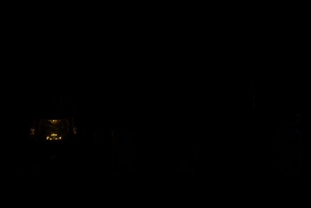
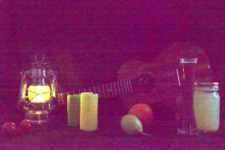
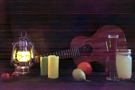
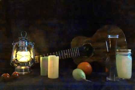
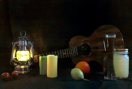
	(a) Short-exposure	(b) Amplified input	(c) BM3D [11]	(d) $G$+$P$ [29]	(e) Paired data [22]	(f) Ours	(g) Long-exposure

Figure 1: Raw denoising results of images from three real-world datasets, i.e., the See-in-the-Dark (SID) dataset [22], the Dark Raw Video (DRV) dataset [28] and our Extreme Low-light Denoising (ELD) dataset, where we present (a) the short-exposure low-light image; (b) amplified noisy input image from (a); (c) the denoised output by the well-known denoising method BM3D [11]; (g) the long-exposure reference image; (d-f) the outputs of UNets [30] trained with (d) synthetic data generated by the signal-dependent heteroscedastic Gaussian noise model (G+P) [29], (e) paired real data of [22, 28], and (f) synthetic data generated by our proposed noise model respectively. All images were converted from raw Bayer space to sRGB for visualization; similarly hereinafter. (Best viewed with zoom)

This paper approaches computational low-light imaging from a fundamental perspective – directly modeling the noise in the imaging procedure of photosensors. Our first observation is that the successful design of denoising algorithms is highly contingent upon the accuracy of the adopted noise model [14, 15, 20, 31]. A precise noise model can not only motivate the design of suitable regularizers for optimization-based methods, but also benefit learning-based algorithms by synthesizing rich realistic training data. Our second observation is the noise pattern are complex and cannot be accurately modeled by existing methods. Even the state-of-the-art heteroscedastic Gaussian noise model [29] cannot delineate the full picture of sensor noise under severely low illuminance. An illustrative example is shown in Figure 1, where the objectionable banding pattern artifacts, an unmodeled noise component that is exacerbated in dim environments, become clearly noticeable by human eyes.

In this work, we mainly focus on the noise formation model for raw images to avoid the impact on noise model from the image processing pipeline (ISP) when converting raw data to sRGB (e.g., gamma correction, gamut mapping, and tone mapping). We propose a physics-based noise formation model for extreme low-light imaging, which explicitly leverages the characteristics of CMOS photosensors to better match the physics of noise formation. As shown in Figure 2, our proposed synthetic pipeline derives from the inherent process of electronic imaging by considering how photons go through several stages, and model sensor noise in a fine-grained manner that includes many noise sources, e.g., photon shot noise, dark current noise, and pixel circuit noise. This yields a comprehensive statistical noise model that can accurately represent various elusive noise-driven phenomena (e.g., the banding pattern artifacts and the color bias issue) in very low light. It also provides a way to decouple the complicated real noise structure into different statistical distributions with clear physical interpretations, which facilitates the understanding of the real noise occurred in extreme low-light conditions.

Furthermore, we devise a method to calibrate the noise parameters from available digital cameras, by first estimating the noise parameters at various ISO settings, then modeling the joint distributions of noise parameters. With this calibration technique, our approach can be easily adapted into any new camera devices at little cost on recording calibration data, thus bypassing the time-consuming paired real training data collection. In order to systematically investigate the generality of our noise model, we additionally introduce an Extreme Low-light Denoising (ELD) dataset taken by various camera devices.

We evaluate our approach on a wide spectrum of low-light imaging applications, including extreme low-light raw denoising, extreme low-light image processing, extreme low-light video denoising as well as several downstream vision applications (i.e., depth estimation, optical flow, object detection/recognition) in the dark. For these tasks, we use the proposed noise model to synthesize training data for deep neural networks. The experiments collectively show that the network trained only with the synthetic data from our noise model can generate highly-accurate denoising results, which are on par with or sometimes even outperform training with real labeled data.

Our main contributions are summarized as follows:

• We formulate a comprehensive noise model that can accurately characterize the real noise structure in the dark. This not only enables us to synthesize realistic noisy images that can match the quality of real data, but also facilitates the understanding of the complicated real noise structure. We demonstrate the usefulness of our noise model on a wide range of low-light imaging applications and show that training deep neural network with it achieves state-of-the-art denoising performance.

• We propose a noise parameter calibration method that can fit our noise model into any given camera devices at various ISO settings. It allows the fast adaptation and deployment of our noise model into any new devices at minimal extra cost, thereby circumventing the labor-intensive paired real data acquisition.

• We collect an extreme low-light denoising dataset ELD which contains images captured by various camera devices under different scenes to verify the effectiveness and generality of the proposed noise model and compare different methods.

The remainder of this paper is organized as follows. In Section 2, we review related low-light imaging methods including both hardware-based approach and computation-based approach. Section 3 introduces our physics-based noise formation model and the noise parameter calibration method for extreme low-light imaging. Both quantitative and qualitative experimental analysis of our approach are provided in Section 4, followed by discussions of applicability scope in Section 5. Conclusions and discussions of open problems are drawn in Section 6. A preliminary version of this work was presented as a conference paper [32].

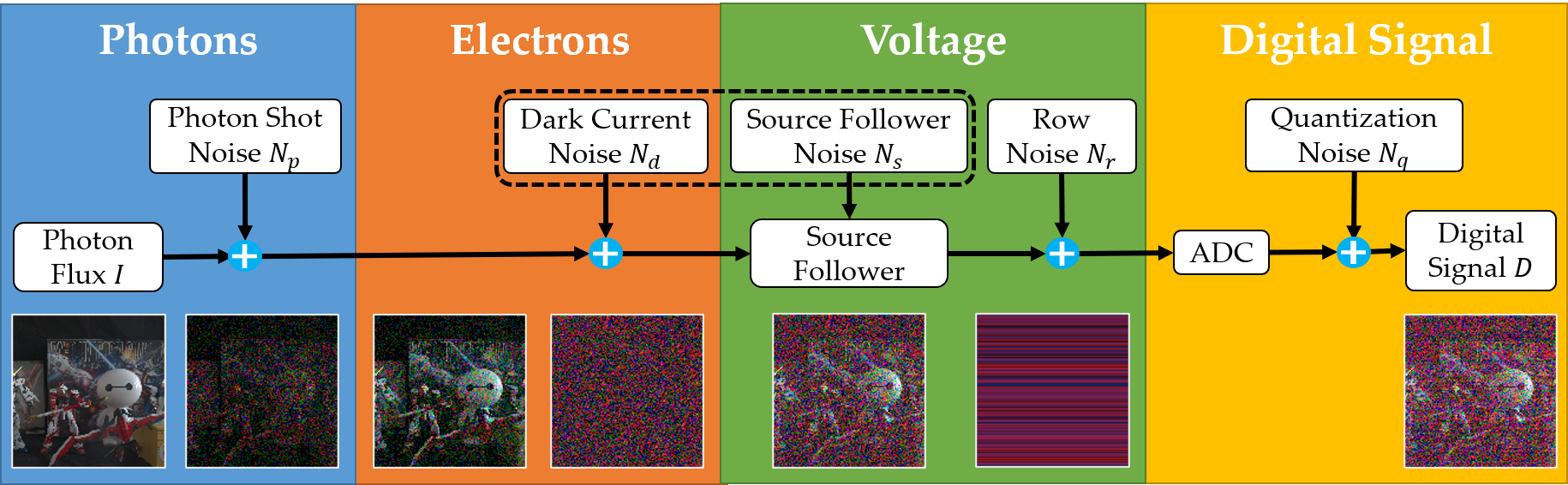
Figure 2: Overview of electronic imaging pipeline and visualization of noise source and resulting image at each stage.

2 Related Work

The challenge of imaging in low light is well-known in the computational photography/imaging community. In this section, we provide an overview of low-light imaging and denoising techniques.

2.1 Hardware-based Approach

Conventional photon detectors i.e., CMOS and CCD photosensors, generally require collecting a large number of photons ($\sim 10^{3}$ photons per pixel) to make a photograph [33, 34], which is largely infeasible in many scientific applications, e.g., non-stellar observation in astronomy [35], remote sensing of human activity from space [36] as well as imaging of delicate biological samples in microscopy [37]. Therefore, many advanced imagers with superior light sensitivity, e.g., EMCCD, ICCD, and sCMOS imagers, have been designed and fabricated to address these imaging challenges [2, 1]. All these imagers could be operated at very low-photon-flux regimes, where moonlight ($\sim$ 10 photons per pixel) could provide sufficient illumination. To further push the limit of low-light imaging, recent years have witnessed significant advancements on ultralow-photon imaging techniques powered by single-photon avalanche diode (SPAD) imagers [3, 4, 5, 6, 7, 8, 9, 10], making imaging under even starlight ($\sim$ 1 photon per pixel) possible.

However, the complex physical mechanism of these hardware-based techniques renders the whole imaging system sophisticated and expensive. Moreover, their applications are often restricted to the laboratory environment, thus are not suitable for consumer-level applications in the wild, e.g., night vision for autonomous vehicles. In this work, we mainly focus on computational low-light imaging using a conventional camera. We demonstrate our method can considerably reduce the number of photons needed by the conventional camera by one to two orders of the magnitude, which even approaches the low-light sensitivity of advanced low-light imagers.

2.2 Computation-based Approach

In contrast to the hardware-based approach, computation-based approaches typically rely on image priors and noise model to reconstruct a high-SNR image from its low-SNR observation acquired by camera. Crafting an analytical regularizer associated with image priors (e.g., smoothness, sparsity, self-similarity, low rank), therefore, plays a critical role in the design pipeline of traditional denoising algorithms [38, 39, 40, 41, 42, 11, 43, 12]. In the modern era, most image denoising algorithms are entirely data-driven, which rely on deep neural networks that implicitly learn the statistical regularities to infer clean images from their noisy counterparts [44, 45, 16, 17, 46, 18, 19, 20]. Although simple and powerful, these learning-based approaches are often trained on synthetic image data due to practical constraints. The most widely-used additive, white, Gaussian noise model deviates strongly from realistic evaluation scenarios, resulting in significant performance declines on photographs with real noise [47, 48].

To step aside the domain gap between synthetic images and real photographs, some works have resorted to collecting paired real data not just for evaluation but for training [48, 22, 49, 28, 50]. Notwithstanding the promising results, collecting sufficient real data with ground-truth labels to prevent overfitting is exceedingly expensive and time-consuming. Recent works exploit the use of paired (Noise2Noise [51]) or single (Noise2Void [52]) noisy images as training data instead of paired noisy and noise-free images. Still, they can not substantially ease the burden of labor requirements for capturing a massive amount of real-world training data.

Another line of research has focused on improving the realism of synthetic training data to circumvent the difficulties in acquiring abundant real data. By considering both photon arrival statistics (“shot” noise) and sensor readout effects (“read” noise), the works of [24, 31] employed a signal-dependent heteroscedastic Gaussian model [29] to characterize the noise properties in raw sensor data. Most recently, [53] proposes a noise model which considers the dynamic streak noise, color channel heterogeneous and clipping effect, to simulate the high-sensitivity noise on real low-light color images. Concurrently, a flow-based generative model [54] is proposed to formulate the distribution of real noise using latent variables with tractable density, and a GAN-based model is presented to learn camera-aware noise model [55]. However, these approaches oversimplify the modern sensor imaging pipeline, especially the noise sources caused by camera electronics, which have been extensively studied in the electronic imaging community [56, 57, 58, 59, 60, 61, 62, 63, 64, 65].

In this work, we propose a physics-based comprehensive noise formation model stemming from the essential process of electronic imaging to synthesize the noisy-image dataset. We show sizeable improvements of denoising performance on real data, particularly under extremely low illuminance.

3 Physics-based Noise Formation Model

The creation of a digital sensor raw image $D$ can be generally formulated by a linear model

$$D=KI+N,$$ (1)

where $I$ is the number of photoelectrons that is proportional to the scene irradiation, $K$ represents the overall system gain composed by analog and digital gains, and $N$ denotes the summation of all noise sources physically caused by light or camera. Under extreme low light, the characteristics of $N$ are formated in terms of the sensor physical process, which is beyond the existing noise models. In the following, we first describe the detailed procedures of the physical formation of a sensor raw image as well as the noise sources introduced during the whole process. An overview of this process is shown in Figure 2.

3.1 Sensor Raw Image Formation

Our photosensor model is primarily based upon the CMOS sensor, which is the dominating imaging sensor nowadays [66]. We consider the electronic imaging pipeline of how incident light is converted from photons to electrons, from electrons to voltage, and finally from voltage to digital numbers, to model noise.

3.1.1 From Photon to Electrons

During exposure, incident lights in the form of photons hit the photosensor pixel area, which liberates photon-generated electrons (photoelectrons) proportional to the light intensity given the photoelectric effect.

Photon shot noise.  Due to the quantum nature of light, there exists an inevitable uncertainty in the number of electrons collected. Such uncertainty imposes a Poisson distribution over this number of electrons, which follows

$$(I+N_{p})\sim\mathcal{P}\left(I\right),$$ (2)

where $N_{p}$ is termed as the photon shot noise and $\mathcal{P}$ denotes the Poisson distribution. This type of noise depends on the signal (i.e., light intensity). Shot noise is a fundamental limitation and cannot be avoided even for a perfect sensor.

There are some other noise sources introduced during the photon-to-electron stage, such as photo response non-uniformity and dark current noise, as reported in the previous literature [57, 58, 64, 59]. Over the last decade, technical advancements in CMOS sensor design and fabrication, e.g., on-sensor dark current suppression, have led to a new generation of digital single lens reflex (DSLR) cameras with lower dark current and better photo response uniformity [67, 68]. Therefore, we assume a constant photo response and absorb the effect of dark current noise $N_{d}$ into read noise $N_{read}$, which will be presented next.

3.1.2 From Electrons to Voltage

After electrons are collected at each site, they are typically integrated, amplified and read out as measurable charge or voltage at the end of exposure time. Noise present during the electrons-to-voltage stage depends on the circuit design and processing technology used, and thus is referred to as pixel circuit noise [58]. It includes thermal noise, reset noise [56], source follower noise [69] and banding pattern noise [58]. The physical origin of these noise components can be found in the electronic imaging literature [56, 58, 64, 69]. For instance, source follower noise is attributed to the action of traps in silicon lattice which randomly capture and emit carriers; banding pattern noise, consisting of row and column artifacts, is associated with the CMOS circuit readout pattern and the amplifier gain mismatch. By leveraging this knowledge, we consider the thermal noise $N_{t}$, source follower noise $N_{s}$ and banding pattern noise $N_{b}$ in our model.

Read noise.  To simplify analysis, we absorb multiple noise sources including dark current noise $N_{d}$, thermal noise $N_{t}$ and source follower noise $N_{s}$ into a unified term, i.e., read noise:

$$N_{read}=N_{d}+N_{t}+N_{s}.$$ (3)

Banding pattern noise $N_{b}$ will be considered later in this section. Read noise is generally assumed to follow a Gaussian distribution, but the analysis of noise data (in Section 3.2) tells a long-tailed nature of its shape. This can be attributed by the flicker and random telegraph signal components of source follower noise [58], or the dark spikes raised by dark current [56]. Therefore, we propose using a statistical distribution that can better characterize the long-tail shape. Specifically, we model the read noise by a Tukey lambda distribution ($TL$) [70], which is a distributional family that can approximate a number of common distributions (e.g., a heavy-tailed Cauchy distribution):

$$N_{read}\sim\mathop{TL}\left(\lambda;0,\sigma_{TL}\right),$$ (4)

where $\lambda$ and $\sigma_{TL}$ indicate the shape and scale parameters respectively, while the location parameter is set to be zero with zero-mean noise assumption.

Color-biased read noise.  Although zero-mean noise assumption is generally applicable in most situations, we find it breaks down under extreme low-light settings, because of the non-negligible direct current (DC) (i.e., zero-frequency) noise component (see Section 3.2). This component originates from the dark current noise, i.e., the averaged number of thermally generated electrons, which renders the noise distribution no longer zero-centered. Though this component has been largely eliminated by the modern on-sensor dark current suppression techniques, e.g., pinned photodiode architecture [71], the residual component is still impactful due to the large system gain $K$ applied to amplify the signal as well as the noise. Even worse, the evaluation (in Section 3.2) reveals this DC noise component varies across color channels, potentially owing to the stack photodiodes design of modern CMOS sensors [72]. Such a color heterogeneous DC component is the culprit that leads to the color bias phenomenon frequently observed under extreme low illuminance (c.f. Figure 1).

To make our noise model simple yet compact, we model the DC noise component (i.e., color bias) as a mean value of the read noise model. As a result, we modify the Equation (4) to

$$N_{read}\sim\mathop{TL}\left(\lambda;\mu_{c},\sigma_{TL}\right),$$ (5)

where $\mu_{c}$ denotes the color-wise DC noise component. The separated analysis of DC component and long-tailed $TL$ distribution will be performed in Section 4.2.

Row noise.  We introduce row noise $N_{r}$ to account for banding pattern noise $N_{b}$. Though $N_{b}$ may appear in images as horizontal or vertical lines, we only consider the row-wise component (horizontal stripes) in our model, as the column-wise counterpart is generally negligible when measuring the noise data (Section 3.2). We simulate the $N_{r}$ by sampling a value from zero-mean Gaussian distribution $\mathcal{N}\left(0,\sigma_{r}\right)$ with scale parameter $\sigma_{r}$ for each row, i.e.,

$$N_{r}\sim\mathcal{N}\left(0,\sigma_{r}\right),$$ (6)

then adding it as an offset to all the pixels within that row.

3.1.3 From Voltage to Digital Numbers

To generate an image that can be stored in a digital storage medium, the analog voltage signal read out during last stage is quantized into discrete codes using an analog-to-digital converter (ADC), which introduces quantization noise.

Quantization noise.  Quantization noise $N_{q}$ is a rounding error between the analog input voltage to the ADC and the output digitized value, which can be assumed to follow a uniform distribution, i.e.,

$$N_{q}\sim U\left(-1/2q,1/2q\right),$$ (7)

where $U(\cdot,\cdot)$ denotes the uniform distribution over the range $[-1/2q,1/2q]$ and $q$ is the quantization step.

To summarize, our noise formation model consists of four major noise components:

$$N=KN_{p}+N_{read}+N_{r}+N_{q},$$ (8)

where $K$, $N_{p}$, $N_{read}$, $N_{r}$ and $N_{q}$ denotes the overall system gain, photon shot noise, read noise, row noise and quantization noise, respectively.

3.2 Sensor Noise Evaluation

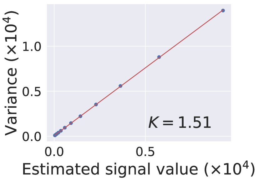
(a) SonyA7S2

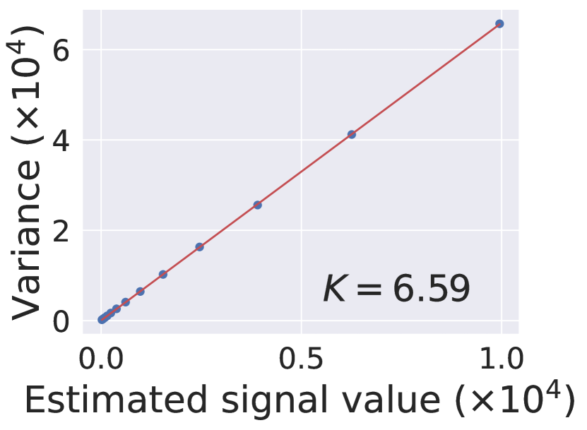
(b) NikonD850

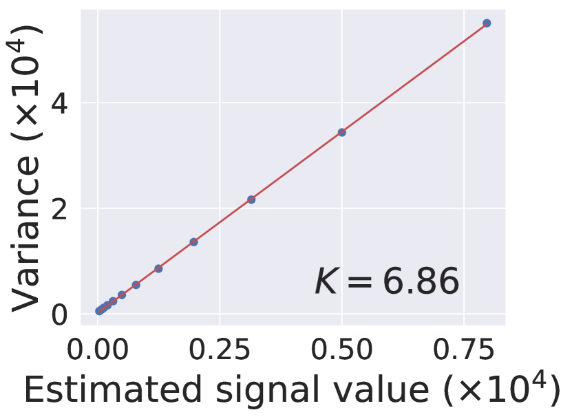
(c) CanonEOS70D

Figure 3: Estimation of the overall system gain $K$ for the three cameras. The noisy signal variance ($y$-axis) and the underlying true signal value ($x$-axis) satisfy a linear function whose slope implies $K$ at the measured ISO (1600) setting.

SonyA7S2 ​​​​
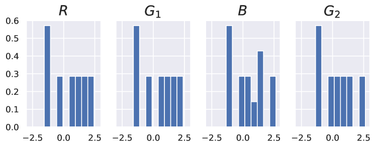
NikonD850 ​​​​
CanonEOS70D ​​​​

Figure 4: Normalized density histogram (with bin size set to 0.5) of the color-wise DC noise component $\mu_{c}$ from different cameras (14-bit depth).

In this section, we present a noise parameter calibration method attached to our proposed noise formation model. Table I summarizes the necessary parameters in our noise model, which include overall system gain $K$ for photon shot noise $N_{p}$, shape and scale parameters ($\lambda$ and $\sigma_{TL}$) for read noise $N_{read}$, $\mu_{c}$ for DC noise component (color bias), and scale parameter $\sigma_{r}$ for row noise $N_{r}$. Given a camera device, our noise calibration method consists of two main procedures: 1) estimating noise parameters at various ISO settings, and 2) modeling joint distributions of noise parameters.

TABLE I: Summary of our noise model

Noise type	Formulation	Parameters
Photon shot noise $N_{p}$	Poisson distribution	System gain $K$
	$(I+N_{p})\sim\mathcal{P}\left(I\right)$
Read noise $N_{read}$	Tukey lambda distribution $N_{read}\sim\mathop{TL}\left(\lambda;\mu_{c},\sigma_{TL}\right)$	Shape $\lambda$
		Color bias $\mu_{c}$
		Scale $\sigma_{TL}$
Row noise $N_{r}$	Gaussian distribution	Scale $\sigma_{r}$
	$N_{r}\sim\mathcal{N}\left(0,\sigma_{r}\right)$
Quantization noise $N_{q}$	Uniform distribution	None
	$N_{q}\sim U\left(-1/2q,1/2q\right)$

3.2.1 Estimating Noise Parameters

Our calibration method makes use of two types of raw images captured at specialized settings, i.e., flat-field frames and bias frames to estimate noise parameters. Flat-field frames are the images captured when sensor is uniformly illuminated. We take them of a white paper on a uniformly-lit wall. The camera is mounted on a tripod close to the paper, and the lens is focused on infinity to diminish non-uniformity. Bias frames are the images captured under a lightless environment with the shortest exposure time. We take them at a dark room and the camera lens is capped-on. Flat-field frames characterize the light-dependent photon shot noise, thus can be used to estimate the related parameter $K$, while bias frames delineate the dark noise picture independent of light, which can be used to derive other noise parameters $\mu_{c}$, $\sigma_{r}$, $\lambda$, $\sigma_{TL}$ sequentially.

Estimate $K$ for photon shot noise.  According to Equation (1) (2) (8), a noisy sensor raw data $D$ can be expressed by

$$D=K(I+N_{p})+N_{o}$$ (9)

where $N_{o}=N_{read}+N_{r}+N_{q}$ accounts for other noise sources independent of light. Following (9), the variance of noisy raw data is given by

$$Var(D)=K^{2}Var(I+N_{p})+Var(N_{o})$$ (10)

where $Var(\cdot)$ denotes the variance operator that calculates the variance of a given random variable. Given that $(I+N_{p})$ follows a Possion distribution, whose variance equals to its mean, we have

$$Var(D) =K^{2}I+Var(N_{o})$$

$$=K(KI)+Var(N_{o})$$ (11)

where $KI$ is the underlying true signal and represented by digital numbers.

Equation (11) reveals a linear relationship between the signal variance $Var(D)$ and the underlying clean digital signal $KI$. Determining $K$, therefore, simply requires fitting a line, if a set of observations ($Var(D)$, $KI$) are accessible to us. Signal variance is easy to calculate, but the true signal value is generally unavailable. By utilizing the flat-field frame, the true signal value $KI$ can be approximated by the median statistics owing to the uniformity. Now we can plot the estimated signal intensity against the variance of the noisy image, and calculate a linear least square regression for these two sets of measurements. As shown in Figure 3, these data points almost perfectly lie in a straight line, whose slope characterizes the overall system gain $K$ at the measured ISO setting of the camera.

Given estimated $K$, we can simulate realistic photon shot noise by firstly convert a raw digital signal $D$ into the number of photoelectrons $I$, then impose a Poisson distribution on it, and finally revert it to $D$.

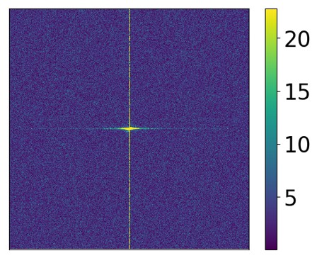
(a) SonyA7S2

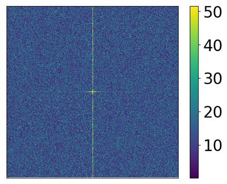
(b) NikonD850

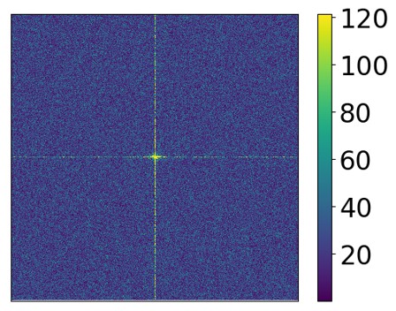
(c) CanonEOS70D

Figure 5: Centralized Fourier spectrum of the bias frames captured by three cameras.

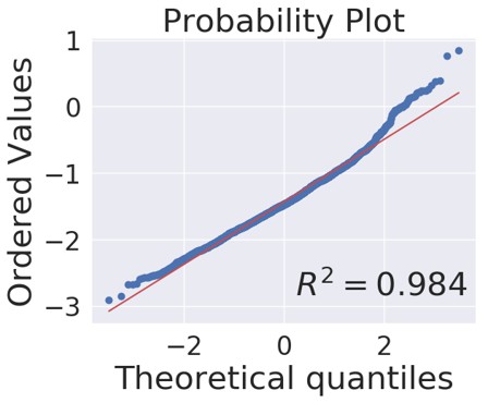
(a) SonyA7S2

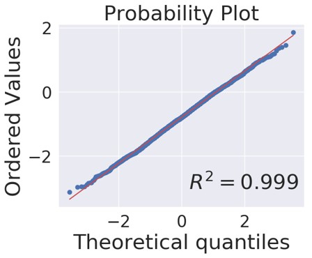
(b) NikonD850

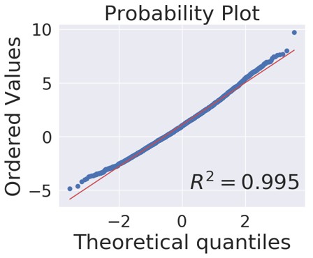
(c) CanonEOS70D

Figure 6: Normal probability plots of row noise data for three cameras. The resulting image looks close to a straight line if the data are approximately normally distributed.

Estimate $\mu_{c}$ for color bias.  Given a bias frame, the DC noise component can be examined by averaging all pixel values within each color channel of the bias frame. If the noise distribution is zero-centered without DC component, the resulting color-wise values should almost equal to the black level (per channel) recorded in the metadata of raw images. However, we find these values are severely biased from the recorded black level, which cannot be explained as random fluctuations caused by other zero-mean noise - this discloses the existence of DC noise component. Figure 4 shows the density histogram of these biases $\mu_{c}$ for each color channel calculated from a number of bias frames. Obvious differences on histogram can be observed among color channels, which demonstrate the varied statistics of DC noise component over color channels.

Note this observation and the new model are very important to extreme low-light denoising, since small bias could lead to severe color shift in extreme low light due to the large digital gain (e.g., $\times$100) applied to signal as well as noise. It challenges the commonly used zero-mean noise assumption, and significantly improves the low-light denoising performance (see Section 4.2).

To exclude the influence of DC noise in the following evaluation of other noise components, the mean values of each color channel are subtracted from the bias frames.

Estimate $\sigma_{r}$ for row noise.  The banding pattern noise can be tested via performing discrete Fourier transform on the bias frame. In Figure 5, the highlighted vertical pattern in the centralized Fourier spectrum reveals the existence of row noise component. To analyze the distribution of row noise, we extract the mean values of each row from raw data. These values, therefore, serve as good estimates to the underlying row noise intensities, given the zero-mean nature of other remaining noise sources. A normal probability plot [73] is drawn in Figure 6, to compare the empirical distribution of row noise with a normal distribution. The normality of the row noise data is also tested by a Shapiro-Wilk test [74]: the resulting $p$-value is higher than $0.05$, suggesting the null hypothesis that the data are normally distributed cannot be rejected. The related scale parameter $\sigma_{r}$ can be easily estimated by maximizing the log-likelihood. The estimated row noise are then removed from the bias frames for the following calibration process.

​​​ SonyA7S2 ​​​​​	​​​	​​​
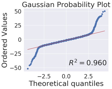
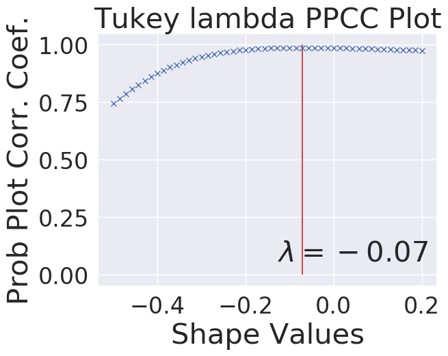
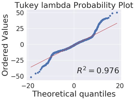
​​​ NikonD850 ​​​​​	​​​	​​​
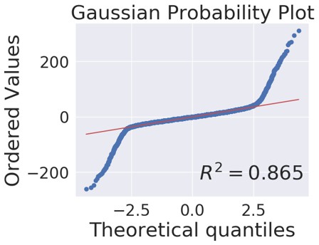
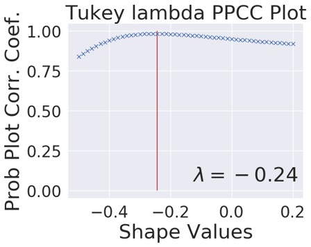
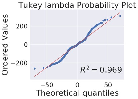
​​​ CanonEOS70D ​​​​​	​​​	​​​

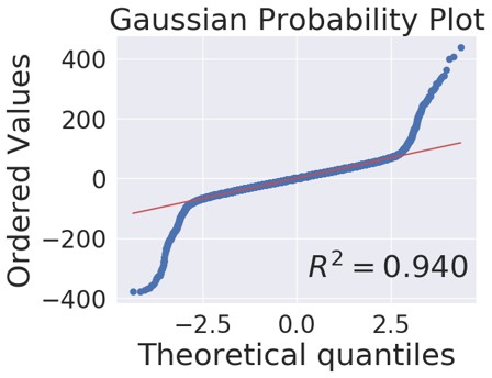
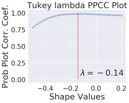
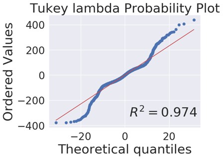
Figure 7: Distribution fitting of read noise for three cameras. Left: probability plot against the Gaussian distribution. Middle: Tukey lambda PPCC plot that determines the optimal $\lambda$ (shown in red line). Right: probability plot against the Tukey Lambda distribution. A higher $R^{2}$ indicates a better fit.

Estimate $\lambda$ and $\sigma_{TL}$ for read noise.  Statistical models can be used to fit the empirical distribution of the residual read noise. A preliminary diagnosis (Figure 7 Left) shows the main body of the data may follow a Gaussian distribution, but it also unveils the long-tail nature of the underlying distribution. In contrast to regarding extreme values as outliers, we observe an appropriate long-tail statistical distribution can characterize the noise data better.

We generate a probability plot correlation coefficient (PPCC) plot [75] to identify a statistical model from a Tukey lambda distributional family [70] that best describes the data. The Tukey lambda distribution is a family of distributions that can approximate many distributions by varying its shape parameter $\lambda$. It can approximate a Gaussian distribution if $\lambda=0.14$, or derive a heavy-tailed distribution if $\lambda<0.14$. The PPCC plot (Figure 7 Middle) is used to find a good value of $\lambda$. The probability plot [73] (Figure 7 Right) is then employed to estimate the scale parameter $\sigma_{TL}$. The goodness-of-fit can be evaluated by $R^{2}$ – the coefficient of determination w.r.t. the resulting probability plot [76]. The $R^{2}$ of the fitted Tukey Lambda distribution is much higher than the Gaussian distribution (e.g., $0.972$ vs. $0.886$), indicating a much better fit to the empirical data.

It should be noted the Poisson mixture model was used in [77] for heavy tail modeling, which utilized two Poisson components to capture the long-tailed behavior of sensor noise. It implicitly imposes a signal/light-dependent nature on noise due to the Poisson model. However, as we found in Figure 7, the long-tailed characteristics is virtually a feature of read noise, which is the noise present at bias frames captured under lightless conditions. It violates the underlying assumption of Poisson mixture model. Consequently, we still adopt the Tukey lambda distribution for long-tailed read noise modeling.

Although we use a unified noise model for different cameras, the noise parameters estimated from different cameras are highly diverse. Figure 7 shows the selected optimal shape parameter $\lambda$ differs camera by camera, implying distributions with varying degree of heavy tails across cameras. The visual comparisons of real and simulated bias frames are presented in Figure 8. Our model is capable of synthesizing realistic noise across various cameras, which outperforms the Gaussian noise model both in terms of the goodness-of-fit measure (i.e., $R^{2}$) and the visual similarity to real noise.

	Real Bias Frame	Gaussian Model	Ours
SonyA7S2
	($R^{2}$)	(0.961)	(0.978)
NikonD850
	($R^{2}$)	(0.880)	(0.972)
CanonEOS70D
	($R^{2}$)	(0.915)	(0.962)

Figure 8: Simulated and real bias frames of three cameras; A higher $R^{2}$ indicates a better fit. (Best viewed with zoom)

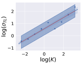
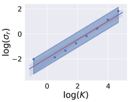
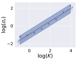
(a) SonyA7S2	(b) NikonD850	(c) CanonEOS70D

Figure 9: Linear least-square fitting from estimated noise parameter samples (blue dots) from three cameras. Upper and lower figures show the joint distributions of $(K,\sigma_{TL})$ and $(K,\sigma_{r})$ respectively, where we sample the noise parameters from the blue shadow regions.

3.2.2 Modeling Joint Parameter Distributions

To choose noise parameters for our noise formation model at various ISO settings, we need to model joint parameter distributions such that the noise parameters can be sampled in a coupled way. Note the system overall gain $K$ is closely related to the ISO setting, so it’s rational to model the joint distributions of $K$ and other noise parameters. As shown in Figure 9, we model the joint distributions of ($K$, $\sigma_{TL}$) and ($K$, $\sigma_{r}$) using the linear least squares method to find the line of best fit for two sets of log-scaled measurements. Our noise parameter sampling procedure is

$$\log\left(K\right)\sim U\left(\log(\hat{K}_{min}),\log(\hat{K}_{max})\right),$$

$$\log\left(\sigma_{TL}\right)|\log\left(K\right)\sim\mathcal{N}\left(a_{TL}\log(K)+b_{TL},\hat{\sigma}_{TL}\right),$$ (12)

$$\log\left(\sigma_{r}\right)|\log\left(K\right)\sim\mathcal{N}\left(a_{r}\log(K)+b_{r},\hat{\sigma}_{r}\right),$$

where $U(\cdot,\cdot)$ denotes a uniform distribution and $\mathcal{N}(\mu,\sigma)$ denotes a Gaussian distribution with mean $\mu$ and standard deviation $\sigma$. $\hat{K}_{min}$ and $\hat{K}_{max}$ are the estimated overall system gains at the minimum and maximum ISO of a camera respectively. $a$ and $b$ indicate the fitted line’s slope and intercept respectively. $\hat{\sigma}$ is an unbiased estimator of standard deviation of the linear regression under the Gaussian error assumption. For shape parameter $\lambda$ and color bias $\mu_{c}$, we simply sample them from the empirical distribution of the estimated parameter samples as we do not observe any clear statistical relationship to $K$ (as well as ISO).

3.2.3 Noisy Image Synthesis

To synthesize noisy images, clean images are chosen and divided by low light factors sampled uniformly from $[100,300]$ to simulate low photon count in the dark. Noise is then generated and added to the scaled clean samples, according to Equation (8) (12). The created noisy images are finally normalized by multiplying the same low light factors to expose bright but excessively noisy contents.

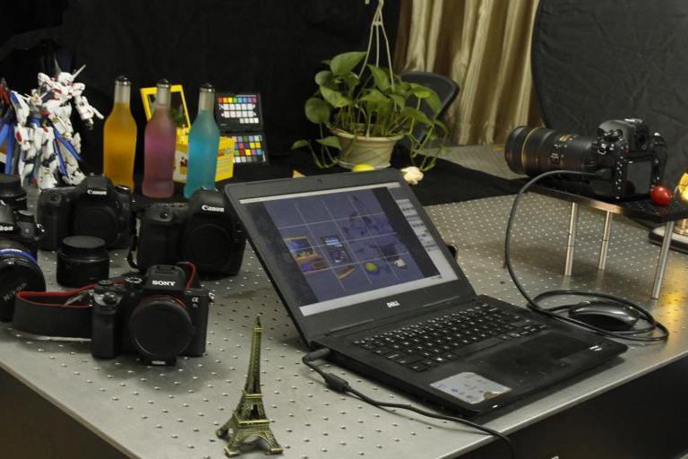
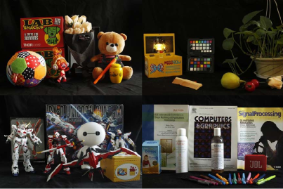
(a) Image capture setup	(b) Sample images

Figure 10: Image capture setup and some sample images from our ELD dataset.

3.3 Extreme Low-light Denoising Dataset (ELD)

To systematically study the generality of the proposed noise formation model, we collect an extreme low-light dataset that covers 10 indoor scenes and 4 camera devices from multiple brands (i.e., SonyA7S2, NikonD850, CanonEOS70D, CanonEOS700D) for benchmarking. We also record bias and flat-field frames for each camera to calibrate our noise model. The data capture setup is shown in Figure 10. The camera is mounted on a sturdy optical table and controlled by a remote software to avoid misalignments caused by camera motion, and the scene is illuminated by natural or direct current light sources to avoid flickering effect of alternating current lights [48, 78]. For each scene of a given camera, a reference image at the base ISO was firstly taken, followed by noisy images whose exposure time was deliberately decreased by low light factors $f$ to simulate extreme low light conditions. Another reference image then was taken akin to the first one, to ensure no accidental errors (e.g., drastic illumination change or accidental camera/scene motion) occurred. The detailed procedures are presented in Algorithm 1. We choose three ISO levels (800, 1600, and 3200) and two low light factors (100, 200) for noisy images to capture our dataset, resulting in 240 (3$\times$2$\times$10$\times$4) raw image pairs in total. The hardest example in our dataset resembles the image captured at a “pseudo” ISO up to 640000 (3200$\times$200).

Algorithm 1 Image capture protocol

0:  $g_{b}=100$; $g_{h}t^{*}=g_{b}t$;

1:  for Each Camera do

2:     for Each Scene do

3:        Meter the scene to find a exposure time $t$ that well exposes the image at the base ISO $g_{b}$;

4:        for Each ISO $g_{h}$ for noisy images do

5:           Take a reference image at exposure setting ($g_{b}$, $t$);

6:           for Each low light factor $f$ do

7:              Capture a noisy image at ($g_{h}$, $t^{*}/f$);

8:           end for

9:           Take another reference image at ($g_{b}$, $t$);

10:        end for

11:     end for

12:  end for

4 Experiments

In this section, we first present the experimental setting including both implementation details and competing methods. Then we conduct comprehensive ablation studies for an in-depth analysis of the noise models and compare our method against prior art. Both quantitative and visual results on various datasets including the new ELD dataset are presented. Finally, we test our approach on low-light videography and several downstream vision tasks (depth estimation, optical flow estimation, object detection/recognition) in the dark.

4.1 Experimental Setting

4.1.1 Implementation Details

To substantiate the effectiveness of our noise formation model, a deep neural network scheme is constructed to perform low-light raw denoising. We utilize the same U-Net architecture [30] as [22]. Raw Bayer images from SID Sony training set are used to create training data. We pack the raw Bayer images into four channels, and crop non-overlapped $512\times 512$ regions augmented by random flipping and rotation. Our approach only uses clean raw images, as the corresponding noisy images are generated by our proposed noise model on-the-fly. Besides, we also train networks based upon other training schemes as references, including training with paired real data (short exposure and long exposure counterpart) and training with paired real noisy images (i.e., Noise2Noise [51]). The whole pipeline of our raw image denoising is depicted in Figure 11 (note the RGB2RGB and raw2RGB experiments in Section 4.5 will use slightly different pipelines).

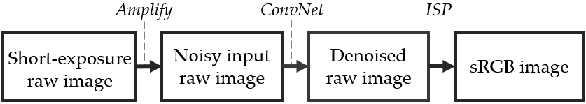
Figure 11: Our raw image denoising pipeline.

Our implementation is based on PyTorch. We train the models with 200 epoch using a simple $L_{1}$ loss and the Adam optimizer [80] with batch size 1. The base learning rate is set to $10^{-4}$ and halved at epoch 100, then reduced to $10^{-5}$ at epoch 180.

4.1.2 Competing Methods

To understand how accurate our proposed noise model would be, we compare our method with

1. the representative non-deep methods, i.e., BM3D [11] and Anscombe-BM3D (A-BM3D) [81];

2. the approaches that use real noisy data for training, i.e., Noise2Noise [51] and “paired real data” [22];

3. the state-of-the-art noise models, i.e., Noiseflow [54] and heteroscedastic Gaussian noise models (G+P) [29].

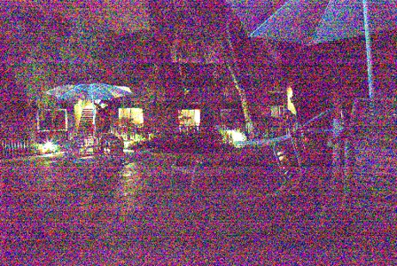
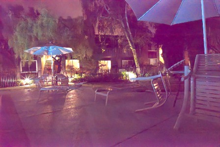
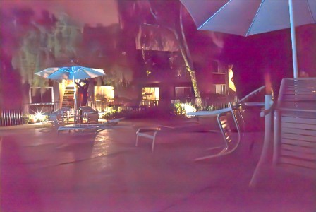
(a) Input	(b) Noise2Noise	(c) Noiseflow	(d) $G$	(e) $G$+$P$	(f) $G$+$P^{*}$
(16.95)	(27.67)	(27.15)	(27.99)	(28.01)	(28.30)
(g) $G^{*}$+$P^{*}$	(h) $G^{*}$+$P^{*}$+$B$	(i) $G^{*}$+$P^{*}$+$B$+$R$	(j) $G^{*}$+$P^{*}$+$B$+$R$+$U$	(k) Paired real data	(l) Reference
(28.41)	(32.03)	(32.20)	(32.25)	(31.81)	(PSNR)

Figure 12: Visual result comparison of different training schemes. Our full noise model ($G^{*}$+$P^{*}$+$B$+$R$+$U$) suppresses the color bias, residual bandings and chroma artifacts compared to other baselines. (Best viewed with zoom)

Input	BM3D	A-BM3D	Noise2Noise	Noiseflow	G+P	Paired real data	Ours
23.08	31.83	31.90	34.30	33.23	34.18	34.48	34.40
26.82	30.66	35.58	33.57	34.54	33.67	37.98	38.67
29.25	35.82	35.81	35.54	35.26	36.10	45.97	47.14
23.87	29.39	28.79	30.12	31.60	29.88	35.31	35.43

Figure 13: Raw image denoising results on both indoor and outdoor scenes from SID Sony dataset. The PSNR value of each resulting image is reported below; similarly hereinafter. (Best viewed on screen with zoom)

For non-deep methods, the noise level parameters required are provided by the off-the-shelf image noise level estimators [29, 82]. We note though there are other non-deep methods [12, 14, 15] that might achieve better results than BM3D, their computation cost is generally unaffordable for large-size images. As for Noiseflow, it requires paired real data to obtain noise data (by subtracting the ground truth images from the noisy ones) for training. We train the Noiseflow model on the SID Sony training dataset, then use the trained model to synthesize noisy dataset for training denoising networks.

4.2 Results on SID Sony Dataset

Single image raw denoising experiment is firstly conducted on SID Sony dataset. The numerical results are reported on whole SID Sony validation and test sets, instead of only indoor scenes in the preliminary version [32]. To account for the imprecisions of shutter speed and analog gain [48], a single scalar is calculated and multiplied into the reconstructed image to minimize the mean square error evaluated by the ground truth.

4.2.1 Ablation Study on Noise Models

To verify the efficacy of the proposed noise model, we compare the performance of networks trained with different noise models developed in Section 3.1. All noise parameters are calibrated using our ELD dataset, and sampled using Equation (12). The results of the other methods described in Section 4.1.2 are also presented as references.

TABLE II: Quantitative Results on Sony set of the SID dataset. $G$: the Gaussian model for read noise $N_{read}$; $G^{*}$: the tukey lambda model for $N_{read}$; $P$: the Gaussian approximation for photon shot noise $N_{p}$; $P^{*}$: the true Poisson model for $N_{p}$; $B$: the color-wise DC model for color bias; $R$: the Gaussian model for row noise $N_{r}$; $U$: the uniform distribution model for quantization noise $N_{q}$. The best and second-best results are indicated by red and blue, respectively.

	$\times 100$	$\times 250$	$\times 300$
Model	​PSNR / SSIM​	​PSNR / SSIM​	​PSNR / SSIM​
BM3D	38.49 / 0.875	34.48 / 0.821	30.98 / 0.766
A-BM3D	39.24 / 0.869	33.74 / 0.742	30.29 / 0.729
Noise2Noise	40.47 / 0.890	35.74 / 0.757	32.34 / 0.707
Noiseflow	41.11 / 0.926	36.97 / 0.838	32.38 / 0.759
Paired real data	42.76 / 0.948	40.59 / 0.935	36.48 / 0.919
$G$	39.47 / 0.866	34.83 / 0.726	31.80 / 0.685
$G$+$P$	40.44 / 0.894	35.67 / 0.773	32.26 / 0.716
$G$+$P^{*}$	41.26 / 0.925	37.27 / 0.849	33.68 / 0.800
$G^{*}$+$P^{*}$	41.64 / 0.936	38.20 / 0.891	34.56 / 0.844
$G^{*}$+$P^{*}$+$B$	42.55 / 0.948	40.44 / 0.930	36.29 / 0.912
$G^{*}$+$P^{*}$+$B$+$R$	42.62 / 0.948	40.55 / 0.930	36.33 / 0.913
$G^{*}$+$P^{*}$+$B$+$R$+$U$	42.75 / 0.949	40.60 / 0.932	36.46 / 0.916

TABLE III: Quantitative results of different methods on our ELD dataset which contains four representative cameras.

Camera	$f$	Index	Non-deep		Training with real data		Training with synthetic data
			​​BM3D [11]​​	​​A-BM3D [81]​​	​​Noise2Noise [51]​​	​​Paired data [22]​​	​​Noiseflow [54]​​	​​G+P [29]​​	​​Ours​​
SonyA7S2	$\times 100$	PSNR	$37.69$	$37.74$	$41.63$	$44.50$	$40.10$	$42.46$	$45.44$
		SSIM	$0.803$	$0.776$	$0.856$	$0.971$	$0.831$	$0.889$	$0.975$
	$\times 200$	PSNR	$34.06$	$35.26$	$37.98$	$42.45$	$37.19$	$38.88$	$43.42$
		SSIM	$0.696$	$0.721$	$0.775$	$0.945$	$0.757$	$0.812$	$0.954$
NikonD850	$\times 100$	PSNR	$33.97$	$36.60$	$40.47$	$41.28$	$40.62$	$40.29$	$42.27$
		SSIM	$0.725$	$0.779$	$0.848$	$0.938$	$0.870$	$0.845$	$0.936$
	$\times 200$	PSNR	$31.36$	$32.59$	$37.98$	$39.44$	$37.61$	$37.26$	$40.36$
		SSIM	$0.618$	$0.723$	$0.820$	$0.910$	$0.805$	$0.786$	$0.908$
CanonEOS70D	$\times 100$	PSNR	$30.79$	$31.88$	$38.21$	$40.10$	$36.69$	$40.94$	$41.20$
		SSIM	$0.589$	$0.692$	$0.826$	$0.931$	$0.787$	$0.934$	$0.949$
	$\times 200$	PSNR	$28.06$	$28.66$	$34.33$	$37.32$	$34.88$	$37.64$	$38.78$
		SSIM	$0.540$	$0.597$	$0.704$	$0.867$	$0.772$	$0.873$	$0.908$
CanonEOS700D	$\times 100$	PSNR	$29.70$	$30.13$	$38.29$	$39.05$	$37.79$	$40.08$	$40.49$
		SSIM	$0.556$	$0.640$	$0.859$	$0.906$	$0.861$	$0.897$	$0.938$
	$\times 200$	PSNR	$27.52$	$27.68$	$34.94$	$36.50$	$35.36$	$37.86$	$38.15$
		SSIM	$0.537$	$0.579$	$0.766$	$0.850$	$0.785$	$0.879$	$0.899$

Input	BM3D	A-BM3D	Noise2Noise	Noiseflow	G+P	Paired real data	Ours
27.95	35.45	35.46	38.81	36.12	40.25	44.53	45.58
28.48	35.73	35.02	41.71	37.40	44.49	46.57	49.51
20.71	29.07	29.02	33.44	33.66	32.93	35.82	37.07
26.57	33.55	36.31	38.31	40.13	38.14	41.89	42.65

Figure 14: Raw image denoising results on our ELD dataset, where we show the visual results on four evaluation scenes. (Best viewed on screen with zoom)

As shown in Table II, the domain gap is significant between the heteroscedastic Gaussian model ($G$+$P$) and the de facto noise model (characterized by the model trained with paired real data). This can be attributed to 1) the Gaussian approximation of Possion distribution is not justified under extreme low illuminance; 2) the long-tail nature of read noise is overlooked; 3) the color-wise DC noise component is not modeled; 4) the horizontal banding noise are not considered in the model. By taking all these factors into account, our final model, i.e., $G^{*}$+$P^{*}$+$B$+$R$+$U$ gives rise to a striking result: the result is comparable to or sometimes even better than the model trained with paired real data. A visual comparison of our final model and other baseline methods is shown in Figure 12, suggesting the effectiveness of our proposed noise formation model.

4.2.2 Method Comparison

The qualitative results of all competing methods on both indoor and outdoor scenes from SID Sony set are presented in Figure 13. It can be seen that the random noise can be suppressed by the model learned with heteroscedastic Gaussian noise (G+P) [29], but the resulting colors are distorted, the banding artifacts become conspicuous, and the image details are barely discernible. Training only with real low-light noisy data is not effective enough, due to the color-bias effect (that violates the zero-mean noise assumption) and the large variance of corruptions (that leads to a large variance of the Noise2Noise solution) [51]. Besides, the learning-based noise model - Noiseflow [54] cannot fully capture the low-light real noise structure, leading to color-shifted and over-smoothed results. By contrast, our model produces visually appealing results as if it had been trained with paired real data.

4.3 Results on our ELD Dataset

4.3.1 Method Comparisons

To see whether our noise model can be applicable to other camera devices as well, we assess model performance on our ELD dataset. Table III and Figure 14 summarize the results of all competing methods on ELD dataset. It can be seen that the non-deep denoising methods, i.e., BM3D and A-BM3D, fail to address the banding residuals, the color bias and the extreme values presented in the noisy input, whereas our model recovers vivid image details, which can be hardly detected from the noisy image by human observers. Moreover, our model trained with synthetic data even often outperforms the model trained with paired real data. We note the finding here conforms with the evaluation of sensor noise presented in Section 3.2, especially in Figure 7 and 8, where we show the underlying noise distribution varies camera by camera. Consequently, training with paired real data from SID Sony camera inevitably overfits to the noise pattern merely existed on the Sony camera, leading to suboptimal results on other types of cameras. In contrast, our model relies on a very flexible noise model and a noise calibration process, making it adapts to noise characteristics of other (calibrated) camera models as well. Additional evidence can be found in Figure 15, where we apply these two models to an image captured by a smartphone camera. Our reconstructed image is clearer and cleaner than what is restored by the model trained with paired real data.

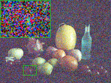
(a) Input

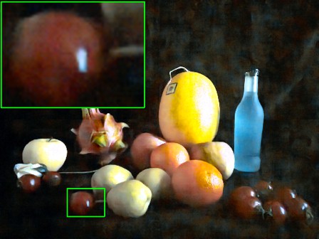
(b) Paired real data

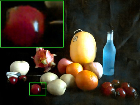
(c) Ours

Figure 15: The denoising results of a low-light image captured by a Huawei Honor 10 camera.

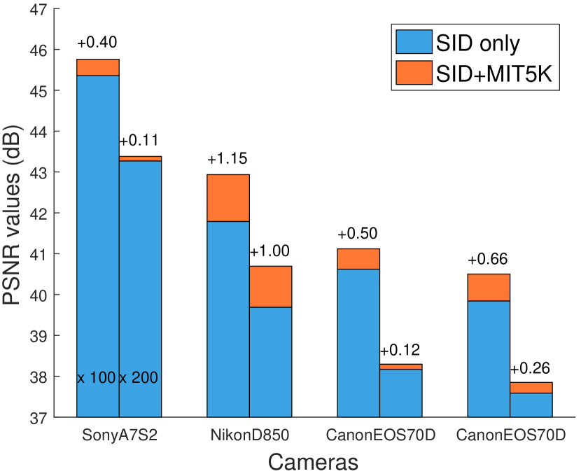
(a)

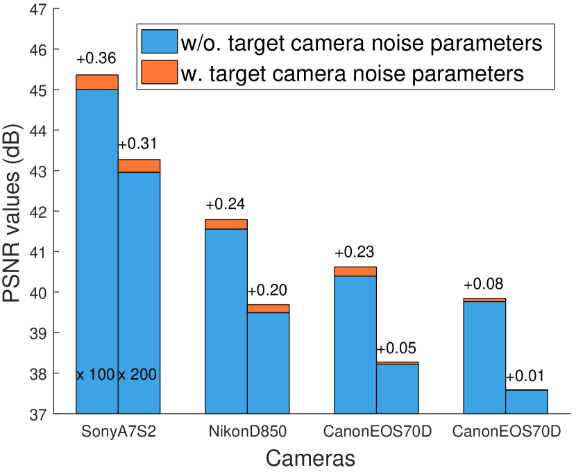
(b)

Figure 16: (a) Performance boost when training with more synthesized data. (b) Noise parameter sensitivity test.

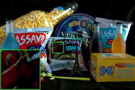
(a) SID only

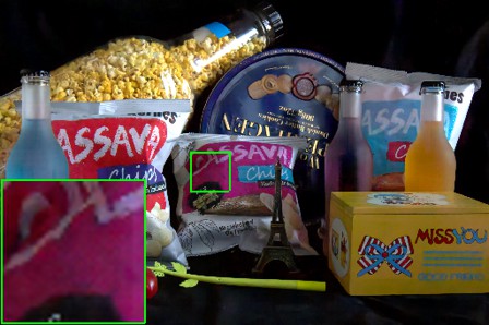
(b) SID + MIT5K

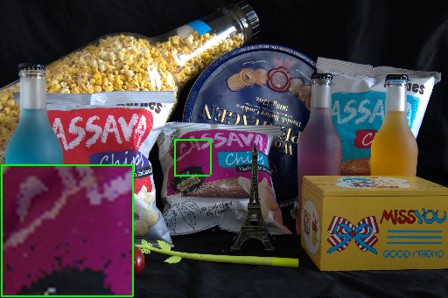
(c) Ground Truth

Figure 17: The recovery results of a low-light image captured by Nikon D850 camera.

4.3.2 Training with More Synthesized Data

A useful merit of our approach compared to training with paired real data, is that our model can be easily incorporated with more real clean samples to train. Figure 16(a) shows the relative improvements of our model when training with the dataset synthesized by additional clean raw images from MIT5K dataset [83]. We find the major improvements are owing to the more accurate color and brightness restoration, as shown in Figure 17. By training with more raw image samples from diverse cameras, the network learns to infer the appearances of pictures more naturally and precisely.

4.3.3 Sensitivity to Noise Calibration

Another benefit of our approach is we only need clean samples and a noise calibration process to adapt to a new camera, in contrast to capturing real noisy images accompanied with densely-labeled ground truth. Besides, the noise calibration process can be simplified once we already have a collection of parameter samples from various cameras. Figure 16(b) shows models can reach comparable performance on target cameras without noise calibration, by simply sampling parameters from other three calibrated cameras instead.

Input	BM3D	A-BM3D	Noise2Noise	G+P	Paired real data	Ours	Reference
29.54	35.54	30.06	35.06	34.53	36.68	36.46	$\infty$
13.50	25.85	27.83	35.70	29.52	36.79	37.65	$\infty$
24.62	31.95	32.87	33.44	32.42	38.50	38.74	$\infty$
25.05	32.27	33.99	32.73	32.24	37.50	37.10	$\infty$

Figure 18: Raw image denoising results on images from SID Fuji dataset. All images are converted from raw X-Trans space to sRGB for visualization. (Best viewed on screen with zoom)

4.4 Applicability to Non-Bayer Raw Data

In the previous sections, we have evaluated our noise formation model on sensor raw images with Bayer color filter array (CFA). Here, we show our noise formation model is also applicable to photosensors with different CFA, e.g., X-Trans used in Fuji cameras. We follow [22] to preprocess the X-Trans raw data by packing it into 9 channels, and create multiple training datasets for different training schemes, based upon the SID Fuji training dataset.

Table IV summarizes the quantitative results of different methods on the SID Fuji testing dataset. As we do not have bias/flat-field frames recorded by the Fuji camera, we simply sample the noise parameters required by noise models using the cameras in our ELD dataset. Even without accurate noise calibration, our final model still reaches a performance comparable to the model trained with paired real data (e.g., 38.33 v.s. 38.56 in $\times 250$). Figure 18 visually compares the results of different methods.

TABLE IV: Quantitative results on Fuji set of SID dataset. Note our results are obtained without noise calibration on the target Fuji camera.

	$\times 100$	$\times 250$	$\times 300$
Model	PSNR / SSIM	PSNR / SSIM	PSNR / SSIM
BM3D	37.26 / 0.889	33.16 / 0.804	30.59 / 0.739
A-BM3D	37.19 / 0.879	30.34 / 0.746	28.92 / 0.678
Noise2Noise	39.03 / 0.893	35.18 / 0.769	33.54 / 0.740
Paired real data	40.13 / 0.958	38.56 / 0.941	37.44 / 0.928
$G$+$P$	38.84 / 0.923	34.86 / 0.815	32.83 / 0.753
Ours	39.88 / 0.959	38.33 / 0.937	37.23 / 0.924

4.5 Applicability to sRGB Denoising

Given a known image processing pipeline (ISP), our noise formation model allows us to generate downstream noise on sRGB space as well, i.e., noisy raw images are firstly generated according to our noise formation model, then are post-processed by a pre-defined ISP to synthesize the final noisy color images. As a proof of concept, here, we assume the color images are finished by a simple ISP with typical functions, including white balance, color correction and a camera response function (CRF). Note that the major goal here is to corroborate the applicability of our noise model to color image denoising. In practice, it can be easily extended into real-world cases when more realistic ISP models for targeted camera devices are accessible (e.g., for camera vendors and/or ISP designers), but this is beyond the scope of this paper.

The necessary parameters to specify some of these operations including the per-channel gain for white balance and the camera-to-sRGB conversion matrix, are directly read from the camera raw files. The CRF is a non-linear mapping to compress a wide range of irradiance values within a fixed range of measurable image intensity values. It often serves as a key feature to distinguish different ISPs [84, 85]. Rather than assuming a standard gamma curve as CRF, we adopt a realistic CRF calibrated on a SonyA7S2 camera (the one used in SID dataset) using a PCA-based radiometric calibration method [85].

TABLE V: Color image (RGB2RGB) denoising results on SID Sony dataset. All the results are evaluated in sRGB space.

	$\times 100$	$\times 250$	$\times 300$
Model	PSNR / SSIM	PSNR / SSIM	PSNR / SSIM
Noise2Noise	19.67 / 0.479	15.11 / 0.332	14.48 / 0.321
Noiseflow	20.77 / 0.512	16.66 / 0.380	15.57 / 0.352
Paired real data	24.63 / 0.598	23.15 / 0.560	22.23 / 0.531
$G$+$P$	21.08 / 0.529	16.64 / 0.390	15.38 / 0.354
Ours	24.45 / 0.599	22.95 / 0.553	21.64 / 0.523

We retrain the networks for color image (i.e., RGB2RGB) denoising based on the same training policy described in Section 4.1.1, except the used raw data have been preprocessed by the pre-defined ISP to produce their color counterparts. As shown in Table V, the network trained with our proposed noise model still reaches a highly competitive performance compared to the network learned with paired real data, indicating the applicability of our model to color image denoising as well.

Moreover, by preparing datasets of both raw and RGB formats, we can train networks to play different roles in the whole low-light imaging pipeline, including raw space denoising as a kind of preprocessing (Raw2Raw), color space denoising as a kind of post-processing (RGB2RGB), and joint performing multiple tasks as a kind of ISP (Raw2RGB) – the networks are learned to do denoising, white balance, color correction and camera response (tone mapping, gamma correction) simultaneously. We compare these three approaches on the SID Sony dataset, using either paired real data or synthetic data generated by our noise model. The quantitative results are shown in Table VI. Interestingly, the approaches of Raw2Raw+ISP and Raw2RGB achieve comparable performance, and outperform the RGB2RGB approach. We note although the Raw2Raw setup is flexible to plug in different ISPs to render different styles of sRGB images, it requires non-blind white balance coefficients, which are often difficult to be deduced in very low light. By contrast, Raw2RGB can automatically infer color constancy from the noisy raw input itself.

TABLE VI: Performance comparison of learning models applied to different stages of the image processing pipeline. We test the same set of noisy images from SID Sony dataset to generate input data of both raw and RGB formats, in which the input RGB images are generated from their corresponding raw counterparts via a pre-defined ISP. The outputs of Raw2Raw are post-processed by the ISP with oracle white balance. All the results are evaluated on sRGB space.

	$\times 100$	$\times 250$	$\times 300$
Model	PSNR / SSIM	PSNR / SSIM	PSNR / SSIM
Paired data
Raw2Raw+ISP	25.37 / 0.600	23.49 / 0.554	22.13 / 0.523
RGB2RGB	24.63 / 0.598	23.15 / 0.560	22.23 / 0.531
Raw2RGB	24.92 / 0.612	23.33 / 0.571	22.69 / 0.547
Ours
Raw2Raw+ISP	24.95 / 0.608	23.60 / 0.560	22.13 / 0.533
RGB2RGB	24.45 / 0.599	22.95 / 0.553	21.64 / 0.523
Raw2RGB	24.65 / 0.605	23.50 / 0.561	22.53 / 0.542

4.6 Applicability to Extreme Low-light Videography

	Input	VBM4D	Noise2Noise	Noiseflow	$G$+$P$	Paired real data	Ours
Frame t
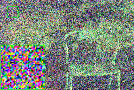
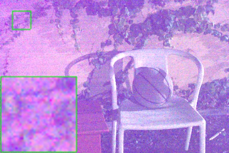
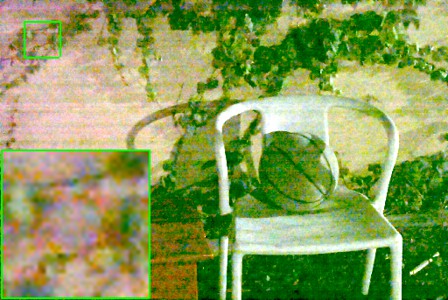
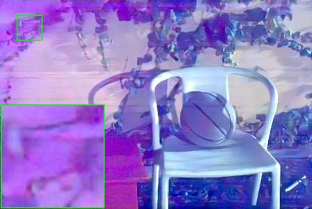
	10.84	21.26	28.11	26.69	30.08	30.97	30.95
t+1
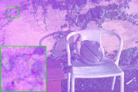
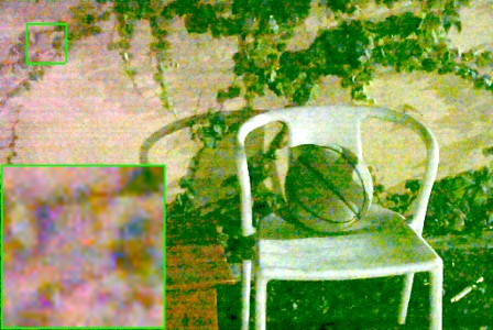
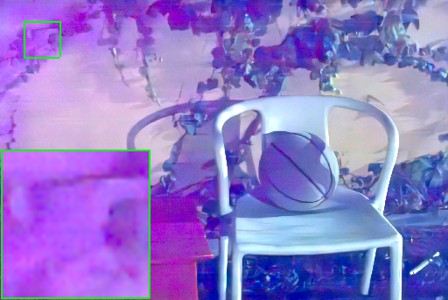
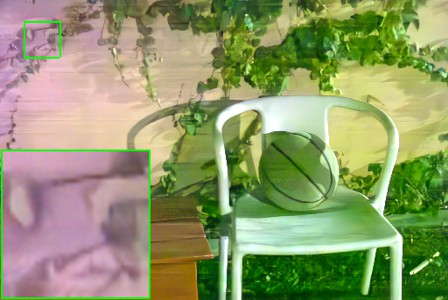
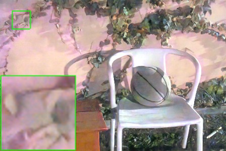
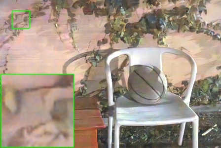
	10.86	21.24	28.20	26.67	30.23	31.20	31.17
t+2
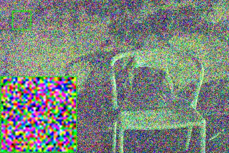
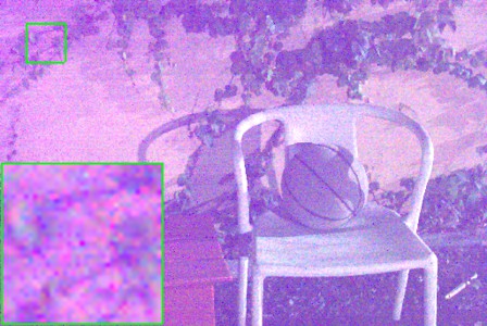
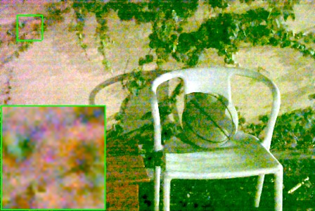
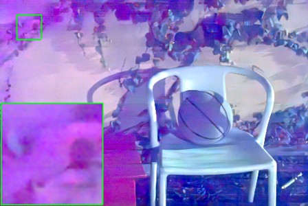
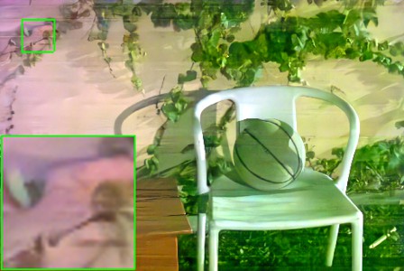
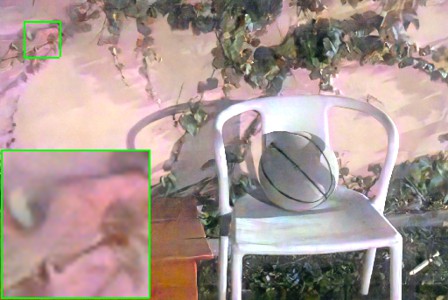
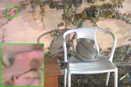
	10.85	21.20	28.14	26.77	30.20	31.01	31.13

Figure 19: Raw video denoising results on static frames from DRV dataset. (Best viewed on screen with zoom)

		Synthetic dynamic video frames			Real dynamic video frames
		Frame T	Frame T+1	Frame T+2	Frame T	Frame T+1	Frame T+2
	Input
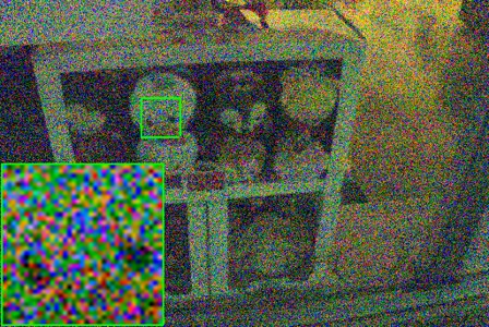
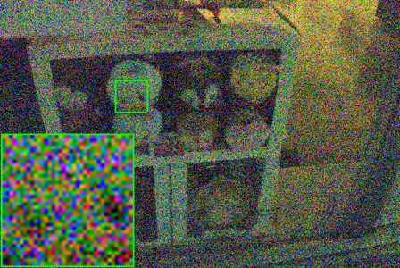
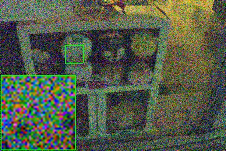
UNet (single-frame)	Paired data
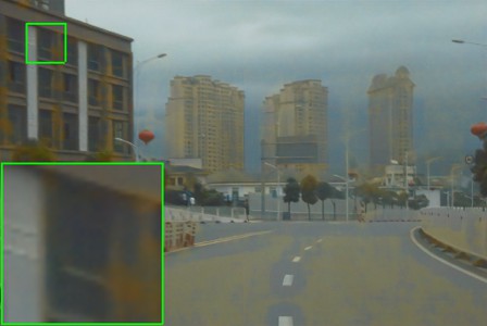
	Ours
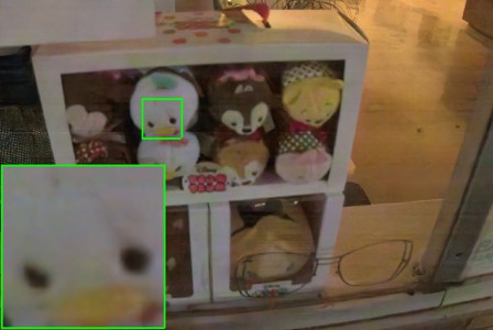
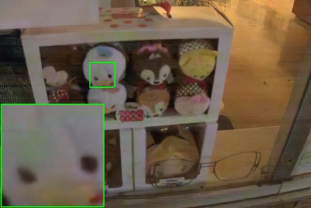
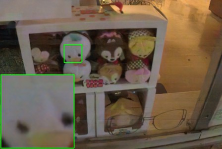
fastDVD (multi-frame)	Paired data (S)
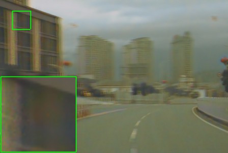
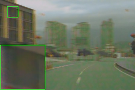
	Ours (S)
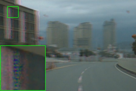
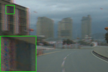
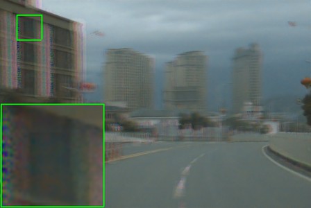
	Ours (D)

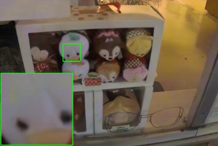
Figure 20: Raw video denoising results on synthetic and real dynamic frames from our dynamic video dataset and DRV dynamic video dataset respectively. “S” and “D” indicate the multi-frame networks are trained on static and dynamic video datasets respectively. (Best viewed on screen with zoom)

TABLE VII: Quantitative results on static video clips from DRV dataset.

Model	PSNR$\uparrow$	SSIM$\uparrow$	ST-RRED$\downarrow$
VBM4D [86]	33.29	0.804	1.568
Noise2Noise [51]	32.73	0.712	0.773
Noiseflow [54]	35.14	0.856	0.441
Paired real data [28]	37.24	0.903	0.369
$G$+$P$ [29]	34.38	0.816	0.467
Ours	36.61	0.896	0.407

TABLE VIII: Quantitative results on synthetic dynamic video clips from our collected dynamic video dataset. “S” and “D” indicate the multi-frame networks are trained on static and dynamic video clips respectively.

Model	PSNR$\uparrow$	SSIM$\uparrow$	ST-RRED$\downarrow$
UNet (single-frame)
Paired real data	33.66	0.925	0.482
Ours	36.40	0.930	0.230
fastDVD (multi-frame)
Paired real data (S)	28.66	0.870	5.746
Ours (S)	28.47	0.860	5.373
Ours (D)	37.48	0.940	0.224

Our approach can be naturally extended into the extreme low-light videography. In this section, we conduct raw video denoising experiment on the Dark Raw Video (DRV) dataset [28]. The DRV training set only contains static videos with corresponding long-exposure ground truth, since collecting paired noisy and noise-free dynamic videos simultaneously is usually impossible. The learning-based video processing pipeline built on [28] uses a sophisticated preprocessing (e.g., $2\times 2$ binning, VBM4D [86] denoising) followed by a U-Net to postprocess videos frame-by-frame. The network is trained on both the recovery loss to encourage the output to be close to the ground truth, as well as the self-consistency loss [28] to enforce the two output frames of the same scene to be similar.

To keep our setting simple, we discard the VBM4D preprocessing, and only use the U-Net with the same loss function as that in [28] to perform raw-to-raw video denoising in a frame-wise manner. The full experimental setting resembles the one used in raw-to-raw image denoising (See Section 4.1) except the extra self-consistency loss for temporal stability. We calibrate our noise model using a Sony RX100 VI camera, the same camera model capturing the DRV dataset. During training, our approach still only need clean raw frames, as we can synthesize arbitrary number of noisy frames to construct paired data. We also implement other training schemes (i.e., Noise2Noise [51], Noiseflow [54], paired real data [28], heteroscedastic Gaussian noise model $G$+$P$ [29]) as baselines based on DRV training dataset, and adopt the same U-Net architecture and loss function for learning.

For each static video, we assess the denoising performance by the averaged PSNR/SSIM over frames (5 continuous frames per video) as well as the Spatio-Temporal Reduced Reference Entropic Differences (ST-RRED) [88]. The ST-RRED is a high performing video quality assessment metrics, which takes both the spatial and temporal distortions into account. Lower ST-RRED score indicates better restoration accuracy. Table VII and Figure 19 display raw video denoising results on DRV testing dataset. It can be seen that our method still arrives at the performance comparable to the “paired real data” model, and produces temporal stable results with less chroma artifacts.

Input	BM3D	Noise2Noise	Noiseflow	G+P	Paired real data	Ours	Reference

Figure 21: Monocular depth estimation in the dark. (Best viewed on screen with zoom)

Input	BM3D	Noise2Noise	Noiseflow	G+P	Paired real data	Ours	Reference

Figure 22: Optical flow in the dark. (Best viewed on screen with zoom)

Input	BM3D	Noise2Noise	Noiseflow	G+P	Paired real data	Ours	Reference

Figure 23: Object detection in the dark. (Best viewed on screen with zoom)

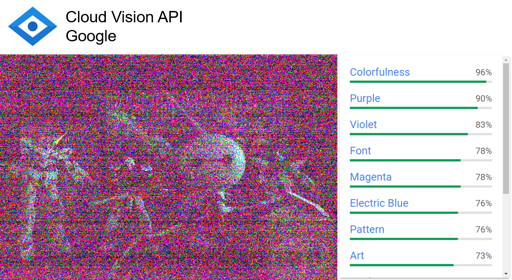
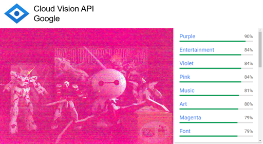
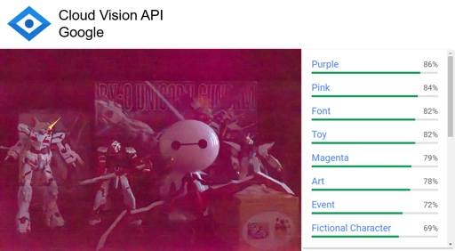
(a) Input	(b) BM3D	(c) Noise2Noise	(d) Noiseflow
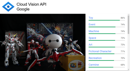
(e) G+P	(f) Paired real data	(g) Ours	(h) Reference

Figure 24: Low-light object recognition results on Google Vision API. (Best viewed on screen with zoom)

It is worthwhile to highlight that our synthetic pipeline allows us to create a paired dynamic video dataset via adding synthetic noise to clean dynamic video frames. This circumvents the difficulty of paired real dynamic video data collection, and makes learning multi-frame denoising networks feasible. To support this argument, we collect 100 clean raw dynamic video clips (5 to 10 frames per clip) using the Sony RX100 VI camera and randomly divide them into 95 clips for training and 5 clips for testing. Both single-frame (U-Net) and multi-frame approaches (FastDVDnet [89]) are compared on dynamic videos. These networks are trained either on paired real data or our synthetic data. Besides, either static video or dynamic video datasets are provided for training FastDVDnet.

Table VIII presents the numerical results on synthetic dynamic video clips, and the visual results on both synthetic and real low-light video frames can be found in Figure 20. It can be seen that the multi-frame network fastDVDnet trained on the static video data cannot generalize to dynamic video frames, since it is impossible to learn motion correspondence based upon only static videos. As a result, it only averages and merges frames, which leads to highly blurry results on dynamic videos. In contrast, the fastDVDnet trained on our synthetic dynamic video dataset performs quite well on dynamic videos, which surpasses the single-frame approaches owing to its additional capability to exploit the temporal correlation over frames.

4.7 Application to Downstream Vision Tasks

We have demonstrated the advantages of our noise model on both low-light photography and videography. Here, we show our approach could also be useful for downstream computer vision applications, e.g., depth estimation in the dark, optical flow in the dark as well as object detection/recognition in the dark. For all these tasks, we follow the same pipeline (Figure 11) to process images, i.e., 1) acquiring an image on RAW format; 2) performing denoising on it; 3) converting it into sRGB domain; 4) executing off-the-shelf vision algorithms on the processed sRGB image. We note in practice, this whole process can be seamlessly integrated into a hardware ISP system executed silently on a chip, such that users do not need to directly interact with RAW formatted images.

State-of-the-art/representative methods are adopted to carry out vision tasks under very limited luminance, including MiDaS [90] for depth estimation, RAFT [91] for optical flow estimation as well as YOLOv5 [92] for object detection. We also test a commercial black-box object recognition solution provided by Google Vision API, which represents a wild uncontrolled task setting. Both visual and numerical results are shown in Figure 21-24 and Table IX respectively, which collectively demonstrate that our low-light denoising algorithm significantly improves the performance of downstream vision applications under extreme low-light settings.

TABLE IX: Quantitative results of downstream vision applications on SID Sony set (depth/detection) and our collected moved scenes (flow). We report the root-mean-square error (RMSE), endpoint error (EPE) and the average number of objects recognized per image (# of Objects) for these three tasks respectively, using the results of long-exposure references as ground truth.

Model​	​Depth​	​Flow​	​Detection​
	(RMSE)	(EPE)	(# of Objects)
Input	0.175	22.44	1.550
BM3D	0.121	15.52	2.496
Noise2Noise	0.120	11.97	3.047
Noiseflow	0.124	11.32	2.837
$G$+$P$	0.122	14.60	3.171
Paired real data	0.091	10.36	3.233
Ours	0.086	8.49	3.434
Reference	0.000	0.00	4.225

5 Discussion of Applicability Scope

Our principal approach can be applied on a variety of real-world application scenarios, ranging from extreme low-light image/video processing to downstream computer vision applications at night. However, it should be clarified the applicability scope here is largely restricted to cases where the RAW images are available. As a result, our method is unfortunately unable to handle some practical situations, e.g., video surveillance from closed-circuit television data, or processing images from internet. Nevertheless, we note RAW image is accessible in many practical and important scenarios from both scientific and industrial domains, where our method is applicable and more desirable. For example, in many scientific imaging applications (e.g., microscopy [37], astronomy [35], remote sensing [36]), what we actually care is to faithfully record the physical world (i.e., the scene irradiance) to analyze and induce physical properties. In such cases, the ISP functionalities in those scientific imagers are either simplified (typically with demosaicking only) or fully disabled, resulting in RAW images that are linearly response to irradiance. Besides, from industrial perspective, our method is also useful for camera and ISP designers with full accessibility to camera RAW and ISP. In this regard, our method could not only facilitate developing scientific imaging solutions, but also help camera/smartphone vendors to enhance their ISP system by inserting our sensor-specific denoising algorithm. It has the potential to unlock the powerful low-light imaging capability on commodity/scientific imagers, which in turn has significant impacts on downstream consumers. Moreover, recent years have witnessed significant advancements on smartphone cameras. Nowadays, almost every mainstream smartphone camera (e.g., iPhone, Huawei, Samsung, etc.) has provided user interface of RAW image acquisition for non-professional users. We envision acquiring RAW images would be more and more convenient in future.

6 Conclusion and Future Work

We have presented a physics-based noise formation model together with a noise parameter calibration method to help resolve the difficulty of extreme low-light imaging. We revisit the electronic imaging pipeline and investigate the influential noise sources overlooked by existing noise models. This enables us to synthesize realistic noisy raw data that match the underlying physical process of noise formation better. We systematically study the efficacy of our noise formation model, by introducing a new dataset that covers four representative camera devices. By training only with our synthetic data, we demonstrate a convolutional neural network can compete with or sometimes even outperform the network trained with paired real data on real-world benchmarks.

Our approach opens a new door to real-world computational low-light imaging, which significantly alleviates the burden of capturing paired real training data from diverse camera devices. It’s highly flexible and enables rapid adaptation and deployment on a variety of consumer-level cameras. Nevertheless, to build a whole computational low-light imaging system, several challenges remain unresolved. For example, both auto-focus and auto-exposure modules would fail under very low light. Their failure will render user experience unfriendly, as taking desired photos with sharp appearance would be excessively difficult. Furthermore, preserving high dynamic range is very appealing for low-light photography. Finally, in many commodity cameras, e.g., smartphone cameras, the computation resource is often very limited. Thus it’s worth investigating light-weight deep architectures specially tailored for low-light image processing as well. We foresee future works to further tackle these challenges and push the boundaries of computational low-light photography.

Kaixuan Wei received the B.S. in Electronic Engineering and the M.S. degree in Computer Science from Beijing Institute of Technology in 2018 and 2021, respectively. His research interests include computer vision, computational photography and computational imaging. He serves as reviewer for major computer vision and machine learning conferences and journals including CVPR/ ICCV/ECCV/AAAI/NeurIPS/ICLR/TPAMI/TIP. He received the Outstanding Paper Award from ICML’20.

Ying Fu received the B.S. degree in Electronic Engineering from Xidian University in 2009, the M.S. degree in Automation from Tsinghua University in 2012, and the Ph.D. degree in information science and technology from the University of Tokyo in 2015. She is currently a professor with the School of Computer Science and Technology, Beijing Institute of Technology. Her research interests include physics-based vision, image and video processing, and computational photography. She received the Outstanding Paper Award from ICML’20.

Yinqiang Zheng received the bachelor’s degree from the Department of Automation, Tianjin University, Tianjin, China, in 2006, the master’s degree in engineering from Shanghai Jiao Tong University, Shanghai, China, in 2009, and the doctoral degree in engineering from the Department of Mechanical and Control Engineering, Tokyo Institute of Technology, Tokyo, Japan, in 2013. After working at National Institute of Informatics, Japan, for more than seven years, he is currently an Associate Professor with The University of Tokyo, Japan. His research interests include image processing, computer vision, and mathematical optimization.

Jiaolong Yang received the B.S. degree in Computer Science from Beijing Institute of Technology in 2010, and the dual Ph.D. degrees in Computer Science and Engineering from the Australian National University and Beijing Institute of Technology in 2016. He is currently a Senior Researcher in the Visual Computing Group at Microsoft Research Asia, Beijing. His research interests include 3D and low-level computer vision. He serves regularly as program committee member/reviewer for major computer vision conferences and journals including CVPR/ ICCV/ECCV/TPAMI/IJCV, and is an Area Chair for CVPR’21, ICCV’21 and CVPR’22. He received the outstanding PhD thesis award from China Society of Image and Graphics in 2017.

References

- [1] D. Dussault and P. Hoess, “Noise performance comparison of iccd with ccd and emccd cameras,” in Proceedings of SPIE - The International Society for Optical Engineering, vol. 5563, 2004, pp. 195–204.
- [2] M. R. Torr, D. Torr, R. Baum, and R. Spielmaker, “Intensified-ccd focal plane detector for space applications: a second generation,” Applied optics, vol. 25, no. 16, pp. 2768–2777, 1986.
- [3] F. Guerrieri, S. Tisa, and F. Zappa, “Fast single-photon imager acquires 1024 pixels at 100 kframe/s,” in Proceedings of SPIE - The International Society for Optical Engineering, vol. 7249, 2009, p. 72490U.
- [4] C. Bruschini, H. Homulle, I. M. Antolovic, S. Burri, and E. Charbon, “Single-photon avalanche diode imagers in biophotonics: review and outlook,” Light: Science & Applications, vol. 8, no. 1, pp. 1–28, 2019.
- [5] A. Kirmani, D. Venkatraman, D. Shin, A. Colaço, F. N. Wong, J. H. Shapiro, and V. K. Goyal, “First-photon imaging,” Science, vol. 343, no. 6166, pp. 58–61, 2014.
- [6] P. A. Morris, R. S. Aspden, J. E. Bell, R. W. Boyd, and M. J. Padgett, “Imaging with a small number of photons,” Nature communications, vol. 6, no. 1, pp. 1–6, 2015.
- [7] G. Gariepy, N. Krstajić, R. Henderson, C. Li, R. R. Thomson, G. S. Buller, B. Heshmat, R. Raskar, J. Leach, and D. Faccio, “Single-photon sensitive light-in-fight imaging,” Nature communications, vol. 6, no. 1, pp. 1–7, 2015.
- [8] D. Shin, F. Xu, D. Venkatraman, R. Lussana, F. Villa, F. Zappa, V. K. Goyal, F. N. Wong, and J. H. Shapiro, “Photon-efficient imaging with a single-photon camera,” Nature communications, vol. 7, no. 1, pp. 1–8, 2016.
- [9] F. Heide, S. Diamond, D. B. Lindell, and G. Wetzstein, “Sub-picosecond photon-efficient 3d imaging using single-photon sensors,” Scientific reports, vol. 8, no. 1, pp. 1–8, 2018.
- [10] M. O’Toole, F. Heide, D. B. Lindell, K. Zang, S. Diamond, and G. Wetzstein, “Reconstructing transient images from single-photon sensors,” in The IEEE Conference on Computer Vision and Pattern Recognition, 2017, pp. 2289–2297.
- [11] K. Dabov, A. Foi, V. Katkovnik, and K. Egiazarian, “Image denoising by sparse 3-d transform-domain collaborative filtering,” IEEE Transactions on Image Processing, vol. 16, no. 8, pp. 2080–2095, 2007.
- [12] S. Gu, Z. Lei, W. Zuo, and X. Feng, “Weighted nuclear norm minimization with application to image denoising,” in The IEEE Conference on Computer Vision and Pattern Recognition, 2014, pp. 2862–2869.
- [13] S. Gu, Y. Li, L. V. Gool, and R. Timofte, “Self-guided network for fast image denoising,” in The IEEE International Conference on Computer Vision, 2019, pp. 2511–2520.
- [14] J. Xu, L. Zhang, D. Zhang, and X. Feng, “Multi-channel weighted nuclear norm minimization for real color image denoising,” in The IEEE International Conference on Computer Vision, 2017, pp. 1105–1113.
- [15] J. Xu, L. Zhang, and D. Zhang, “A trilateral weighted sparse coding scheme for real-world image denoising,” in The European Conference on Computer Vision, 2018, pp. 20–36.
- [16] X. Mao, C. Shen, and Y.-B. Yang, “Image restoration using very deep convolutional encoder-decoder networks with symmetric skip connections,” in Advances in Neural Information Processing Systems, 2016, pp. 2802–2810.
- [17] K. Zhang, W. Zuo, Y. Chen, D. Meng, and L. Zhang, “Beyond a gaussian denoiser: Residual learning of deep cnn for image denoising,” IEEE Transactions on Image Processing, vol. 26, no. 7, pp. 3142–3155, 2017.
- [18] Y. Tai, J. Yang, X. Liu, and C. Xu, “Memnet: A persistent memory network for image restoration,” in The IEEE International Conference on Computer Vision, 2017, pp. 4549–4557.
- [19] C. Chen, Z. Xiong, X. Tian, and F. Wu, “Deep boosting for image denoising,” in The European Conference on Computer Vision, 2018, pp. 3–19.
- [20] S. Guo, Z. Yan, K. Zhang, W. Zuo, and L. Zhang, “Toward convolutional blind denoising of real photographs,” in The IEEE Conference on Computer Vision and Pattern Recognition, 2019, pp. 1712–1722.
- [21] S. Anwar and N. Barnes, “Real image denoising with feature attention,” in The IEEE International Conference on Computer Vision, 2019, pp. 3155–3164.
- [22] C. Chen, Q. Chen, J. Xu, and V. Koltun, “Learning to see in the dark,” in The IEEE Conference on Computer Vision and Pattern Recognition, 2018, pp. 3291–3300.
- [23] Z. Liu, Y. Lu, X. Tang, M. Uyttendaele, and S. Jian, “Fast burst images denoising,” ACM Transactions on Graphics, vol. 33, no. 6, pp. 1–9, 2014.
- [24] B. Mildenhall, J. T. Barron, J. Chen, D. Sharlet, R. Ng, and R. Carroll, “Burst denoising with kernel prediction networks,” in The IEEE Conference on Computer Vision and Pattern Recognition, 2018, pp. 2502–2510.
- [25] S. W. Hasinoff, D. Sharlet, R. Geiss, A. Adams, and M. Levoy, “Burst photography for high dynamic range and low-light imaging on mobile cameras,” ACM Transactions on Graphics, vol. 35, no. 6, p. 192, 2016.
- [26] O. Liba, K. Murthy, Y.-T. Tsai, T. Brooks, T. Xue, N. Karnad, Q. He, J. T. Barron, D. Sharlet, R. Geiss et al., “Handheld mobile photography in very low light,” ACM Transactions on Graphics, vol. 38, no. 6, pp. 1–16, 2019.
- [27] Z. Xia, F. Perazzi, M. Gharbi, K. Sunkavalli, and A. Chakrabarti, “Basis prediction networks for effective burst denoising with large kernels,” in The IEEE Conference on Computer Vision and Pattern Recognition, 2020, pp. 11 841–11 850.
- [28] C. Chen, Q. Chen, M. N. Do, and V. Koltun, “Seeing motion in the dark,” in The IEEE International Conference on Computer Vision, 2019, pp. 3184–3193.
- [29] A. Foi, M. Trimeche, V. Katkovnik, and K. Egiazarian, “Practical poissonian-gaussian noise modeling and fitting for single-image raw-data,” IEEE Transactions on Image Processing, vol. 17, no. 10, pp. 1737–1754, 2008.
- [30] O. Ronneberger, P. Fischer, and T. Brox, “U-net: Convolutional networks for biomedical image segmentation,” in International Conference on Medical image computing and computer-assisted intervention, 2015, pp. 234–241.
- [31] T. Brooks, B. Mildenhall, T. Xue, J. Chen, D. Sharlet, and J. T. Barron, “Unprocessing images for learned raw denoising,” in The IEEE Conference on Computer Vision and Pattern Recognition, 2019, pp. 11 028–11 037.
- [32] K. Wei, Y. Fu, J. Yang, and H. Huang, “A physics-based noise formation model for extreme low-light raw denoising,” in The IEEE Conference on Computer Vision and Pattern Recognition, 2020, pp. 2755–2764.
- [33] G. C. Holst, “Ccd arrays, cameras, and displays,” 1998.
- [34] P. Llull, X. Liao, X. Yuan, J. Yang, D. Kittle, L. Carin, G. Sapiro, and D. J. Brady, “Coded aperture compressive temporal imaging,” Optics express, vol. 21, no. 9, pp. 10 526–10 545, 2013.
- [35] I. S. McLean, Electronic imaging in astronomy: detectors and instrumentation. Springer Science and Business Media, 2008.
- [36] N. Levin, C. C. Kyba, Q. Zhang, A. S. de Miguel, M. O. Román, X. Li, B. A. Portnov, A. L. Molthan, A. Jechow, S. D. Miller et al., “Remote sensing of night lights: A review and an outlook for the future,” Remote Sensing of Environment, vol. 237, p. 111443, 2020.
- [37] M. S. Joens, C. Huynh, J. M. Kasuboski, D. Ferranti, Y. J. Sigal, F. Zeitvogel, M. Obst, C. J. Burkhardt, K. P. Curran, S. H. Chalasani et al., “Helium ion microscopy (him) for the imaging of biological samples at sub-nanometer resolution,” Scientific reports, vol. 3, p. 3514, 2013.
- [38] L. I. Rudin, S. Osher, and E. Fatemi, “Nonlinear total variation based noise removal algorithms,” Physica D Nonlinear Phenomena, vol. 60, no. 1–4, pp. 259–268, 1992.
- [39] S. Osher, M. Burger, D. Goldfarb, J. Xu, and W. Yin, “An iterative regularization method for total variation-based image restoration,” Multiscale Modeling and Simulation, vol. 4, no. 2, pp. 460–489, 2005.
- [40] M. Elad and M. Aharon, “Image denoising via sparse and redundant representations over learned dictionaries,” IEEE Transactions on Image Processing, vol. 15, no. 12, pp. 3736–3745, 2006.
- [41] W. Dong, X. Li, L. Zhang, and G. Shi, “Sparsity-based image denoising via dictionary learning and structural clustering,” in The IEEE Conference on Computer Vision and Pattern Recognition. IEEE, 2011, pp. 457–464.
- [42] J. Mairal, M. Elad, and G. Sapiro, “Sparse representation for color image restoration,” IEEE Transactions on Image Processing, vol. 17, no. 1, pp. 53–69, 2008.
- [43] A. Buades, B. Coll, and J.-M. Morel, “A non-local algorithm for image denoising,” in The IEEE Conference on Computer Vision and Pattern Recognition, 2005, pp. 60–65.
- [44] U. Schmidt and S. Roth, “Shrinkage fields for effective image restoration,” in The IEEE Conference on Computer Vision and Pattern Recognition, 2014, pp. 2774–2781.
- [45] Y. Chen, W. Yu, and T. Pock, “On learning optimized reaction diffusion processes for effective image restoration,” in The IEEE Conference on Computer Vision and Pattern Recognition, 2015, pp. 5261–5269.
- [46] M. Gharbi, G. Chaurasia, S. Paris, and F. Durand, “Deep joint demosaicking and denoising,” ACM Transactions on Graphics, vol. 35, no. 6, pp. 191:1–191:12, 2016.
- [47] T. Plotz and S. Roth, “Benchmarking denoising algorithms with real photographs,” in The IEEE Conference on Computer Vision and Pattern Recognition, 2017, pp. 2750–2759.
- [48] A. Abdelhamed, S. Lin, and M. S. Brown, “A high-quality denoising dataset for smartphone cameras,” in The IEEE Conference on Computer Vision and Pattern Recognition, 2018, pp. 1692–1700.
- [49] E. Schwartz, R. Giryes, and A. M. Bronstein, “Deepisp: Learning end-to-end image processing pipeline,” IEEE Transactions on Image Processing, vol. PP, no. 99, pp. 1–1, 2018.
- [50] H. Jiang and Y. Zheng, “Learning to see moving objects in the dark,” in The IEEE International Conference on Computer Vision, 2019, pp. 7323–7332.
- [51] J. Lehtinen, J. Munkberg, J. Hasselgren, S. Laine, T. Karras, M. Aittala, and T. Aila, “Noise2noise: Learning image restoration without clean data,” in International Conference on Machine Learning, 2018, pp. 2971–2980.
- [52] A. Krull, T.-O. Buchholz, and F. Jug, “Noise2void - learning denoising from single noisy images,” in The IEEE Conference on Computer Vision and Pattern Recognition, 2019, pp. 2124–2132.
- [53] W. Wang, X. Chen, C. Yang, X. Li, X. Hu, and T. Yue, “Enhancing low light videos by exploring high sensitivity camera noise,” in The IEEE International Conference on Computer Vision, 2019, pp. 4110–4118.
- [54] A. Abdelhamed, M. A. Brubaker, and M. S. Brown, “Noise flow: Noise modeling with conditional normalizing flows,” in The IEEE International Conference on Computer Vision, 2019, pp. 3165–3173.
- [55] K.-C. Chang, R. Wang, H.-J. Lin, Y.-L. Liu, C.-P. Chen, Y.-L. Chang, and H.-T. Chen, “Learning camera-aware noise models,” in The European Conference on Computer Vision, 2020, pp. 343–358.
- [56] M. V. Konnik and J. S. Welsh, “High-level numerical simulations of noise in ccd and cmos photosensors: review and tutorial.” arXiv preprint arXiv:1412.4031, 2014.
- [57] G. E. Healey and R. Kondepudy, “Radiometric ccd camera calibration and noise estimation,” IEEE Transactions on Pattern Analysis and Machine Intelligence, vol. 16, no. 3, pp. 267–276, 1994.
- [58] R. D. Gow, D. Renshaw, K. Findlater, L. Grant, S. J. Mcleod, J. Hart, and R. L. Nicol, “A comprehensive tool for modeling cmos image-sensor-noise performance,” IEEE Transactions on Electron Devices, vol. 54, no. 6, pp. 1321–1329, 2007.
- [59] R. L. Baer, “A model for dark current characterization and simulation,” vol. 6068, 2006, pp. 37–48.
- [60] A. El Gamal and H. Eltoukhy, “Cmos image sensors,” IEEE Circuits and Devices Magazine, vol. 21, no. 3, pp. 6–20, 2005.
- [61] J. Farrell, M. Okincha, and M. Parmar, “Sensor calibration and simulation,” in Proceedings of SPIE - The International Society for Optical Engineering, vol. 6817, 2008, pp. 249–257.
- [62] K. Irie, A. E. Mckinnon, K. Unsworth, and I. M. Woodhead, “A technique for evaluation of ccd video-camera noise,” IEEE Transactions on Circuits and Systems for Video Technology, vol. 18, no. 2, pp. 280–284, 2008.
- [63] R. A. Boie and I. J. Cox, “An analysis of camera noise,” IEEE Transactions on Pattern Analysis and Machine Intelligence, vol. 14, no. 6, pp. 671–674, 1992.
- [64] H. Wach and E. R. D. Jr, “Noise modeling for design and simulation of computational imaging systems,” vol. 5438, 2004, pp. 159–170.
- [65] R. Costantini and S. Susstrunk, “Virtual sensor design,” vol. 5301, 2004, pp. 408–419.
- [66] G. V. Research, “Image sensors market analysis,” 2016. [online].” http://www.grandviewresearch.com/industry-analysis/imagesensors-market, 2016.
- [67] E. R. Fossum and D. B. Hondongwa, “A review of the pinned photodiode for ccd and cmos image sensors,” IEEE Journal of the Electron Devices Society, vol. 2, no. 3, pp. 33–43, 2014.
- [68] W. Lin, G. Sung, and J. Lin, “High performance cmos light detector with dark current suppression in variable-temperature systems,” Sensors, vol. 17, no. 1, p. 15, 2016.
- [69] C. Leyris, A. Hoffmann, M. Valenza, J.-C. Vildeuil, and F. Roy, “Trap competition inducing r.t.s noise in saturation range in n-mosfets,” in Proceedings of SPIE - The International Society for Optical Engineering, vol. 5844, 2005, pp. 41–51.
- [70] B. L. Joiner and J. R. Rosenblatt, “Some properties of the range in samples from tukey’s symmetric lambda distributions,” Publications of the American Statistical Association, vol. 66, no. 334, pp. 394–399, 1971.
- [71] R. N. Clark, “On-sensor dark current suppression technology dark frames are no longer necessary,” https://clarkvision.com/articles/dark-current-suppression-technology/, 2016.
- [72] D. L. Gilblom, S. K. Yoo, and P. Ventura, “Real-time color imaging with a cmos sensor having stacked photodiodes,” in Ultrahigh-and High-Speed Photography, Photonics, and Videography, vol. 5210, 2004, pp. 105–115.
- [73] M. B. Wilk and R. Gnanadesikan, “Probability plotting methods for the analysis of data,” Biometrika, vol. 55, no. 1, pp. 1–17, 1968.
- [74] S. S. Shapiro and R. S. Francia, “An approximate analysis of variance test for normality,” Biometrika, vol. 67, no. 337, pp. 215–216, 1975.
- [75] J. J. Filliben, “The probability plot correlation coefficient test for normality,” Technometrics, vol. 17, no. 1, pp. 111–117, 1975.
- [76] E. C. Morgan, M. Lackner, R. M. Vogel, and L. G. Baise, “Probability distributions for offshore wind speeds,” Energy Conversion and Management, vol. 52, no. 1, pp. 15 – 26, 2011.
- [77] J. Zhang and K. Hirakawa, “Improved denoising via poisson mixture modeling of image sensor noise,” IEEE Transactions on Image Processing, vol. 26, no. 4, pp. 1565–1578, 2017.
- [78] M. Sheinin, Y. Y. Schechner, and K. N. Kutulakos, “Computational imaging on the electric grid,” in The IEEE Conference on Computer Vision and Pattern Recognition, 2017, pp. 2363–2372.
- [79] R. N. Clark, “Exposure and digital cameras, part 1: What is iso on a digital camera? when is a camera isoless? iso myths and digital cameras,” http://www.clarkvision.com/articles/iso/, 2012.
- [80] D. P. Kingma and J. Ba, “Adam: A method for stochastic optimization,” in International Conference on Learning Representations, 2015.
- [81] M. Makitalo and A. Foi, “Optimal inversion of the anscombe transformation in low-count poisson image denoising,” IEEE Transactions on Image Processing, vol. 20, no. 1, pp. 99–109, 2011.
- [82] G. Chen, F. Zhu, and P. Ann Heng, “An efficient statistical method for image noise level estimation,” in The IEEE International Conference on Computer Vision, 2015, pp. 477–485.
- [83] V. Bychkovsky, S. Paris, E. Chan, and F. Durand, “Learning photographic global tonal adjustment with a database of input / output image pairs,” in The IEEE Conference on Computer Vision and Pattern Recognition, 2011, pp. 97–104.
- [84] S. J. Kim, H. T. Lin, Z. Lu, S. Süsstrunk, S. Lin, and M. S. Brown, “A new in-camera imaging model for color computer vision and its application,” IEEE Transactions on Pattern Analysis and Machine Intelligence, vol. 34, no. 12, pp. 2289–2302, 2012.
- [85] M. D. Grossberg and S. K. Nayar, “Modeling the space of camera response functions,” IEEE Transactions on Pattern Analysis and Machine Intelligence, vol. 26, no. 10, pp. 1272–1282, 2004.
- [86] M. Maggioni, G. Boracchi, A. Foi, and K. Egiazarian, “Video denoising, deblocking, and enhancement through separable 4-d nonlocal spatiotemporal transforms,” IEEE Transactions on Image Processing, vol. 21, no. 9, pp. 3952–3966, 2012.
- [87] K. Simonyan and A. Zisserman, “Very deep convolutional networks for large-scale image recognition,” arXiv preprint arXiv:1409.1556, 2014.
- [88] R. Soundararajan and A. C. Bovik, “Video quality assessment by reduced reference spatio-temporal entropic differencing,” IEEE Transactions on Circuits and Systems for Video Technology, vol. 23, no. 4, pp. 684–694, 2012.
- [89] M. Tassano, J. Delon, and T. Veit, “Fastdvdnet: Towards real-time deep video denoising without flow estimation,” in The IEEE Conference on Computer Vision and Pattern Recognition, 2020, pp. 1351–1360.
- [90] R. Ranftl, K. Lasinger, D. Hafner, K. Schindler, and V. Koltun, “Towards robust monocular depth estimation: Mixing datasets for zero-shot cross-dataset transfer,” IEEE Transactions on Pattern Analysis and Machine Intelligence, 2020.
- [91] Z. Teed and J. Deng, “Raft: Recurrent all-pairs field transforms for optical flow,” in European Conference on Computer Vision, 2020, pp. 402–419.
- [92] G. Jocher, A. Stoken, and J. Borovec, “YOLOv5,” 2021. [Online]. Available: https://doi.org/10.5281/zenodo.4418161