Statistical Analysis of Wasserstein Distributionally Robust Estimators

Jose Blanchet Management Science & Engineering, Stanford University, CA 94305, jose.blanchet@stanford.edu Karthyek Murthy Singapore University of Technology and Design, Singapore 487372, karthyek_murthy@sutd.edu.sg Viet Anh Nguyen Management Science & Engineering, Stanford University, CA 94305 and VinAI Research, Vietnam, viet-anh.nguyen@stanford.edu

Blanchet, Murthy and Nguyen: Statistical Analysis of Wasserstein Distributionally Robust Estimators

We consider statistical methods which invoke a min-max distributionally robust formulation to extract good out-of-sample performance in data-driven optimization and learning problems. Acknowledging the distributional uncertainty in learning from limited samples, the min-max formulations introduce an adversarial inner player to explore unseen covariate data. The resulting Distributionally Robust Optimization (DRO) formulations, which include Wasserstein DRO formulations (our main focus), are specified using optimal transportation phenomena. Upon describing how these infinite-dimensional min-max problems can be approached via a finite-dimensional dual reformulation, the tutorial moves into its main component, namely, explaining a generic recipe for optimally selecting the size of the adversary’s budget. This is achieved by studying the limit behavior of an optimal transport projection formulation arising from an inquiry on the smallest confidence region that includes the unknown population risk minimizer. Incidentally, this systematic prescription coincides with those in specific examples in high-dimensional statistics and results in error bounds that are free from the curse of dimensions. Equipped with this prescription, we present a central limit theorem for the DRO estimator and provide a recipe for constructing compatible confidence regions that are useful for uncertainty quantification. The rest of the tutorial is devoted to insights into the nature of the optimizers selected by the min-max formulations and additional applications of optimal transport projections.

statistical estimators, Wasserstein distance, optimal transport, distributionally robust optimization

1 Introduction

Data-driven decision making has permeated virtually every aspect of operations research (OR) and management science (MS). This proliferation has been made possible thanks to our increased ability to collect a gigantic amount of data and the availability of computational resources which enable the solution of complex uncertainty-informed optimization problems. In many OR/MS tasks, decisions are chosen as prescriptions to improve future performance. Hence, it is imperative to recognize that the available evidence (often based on the limited data collected from previous experience or presumably similar environments) might deflect from the future environment in which the decision will be applied. This recognition ignites the field of decision making under uncertainty, and an emerging framework for robust decision making and statistical analysis is that of distributionally robust optimization (DRO).

While DRO formulations have received substantial attention in the OR/MS community during the last decades [5, 94, 82, 20, 89, 70, 71], recent years have witnessed a significant amount of interest in statistical properties of data-driven DRO-based decision rules and associated inference obtained by these of decisions. The main goal of this tutorial is to discuss some statistical properties enjoyed by decisions obtained from DRO formulations as well as the associated techniques that are used to analyze these types of decisions. Our focus is on DRO formulations for which the uncertainty region is described in terms of so-called optimal transport discrepancies (which include the Wasserstein distances as special cases).

The literature that connects optimal transport and data analytics has grown substantially in recent years. The text [69] provides many examples in which optimal transport is used in areas such as computer vision and machine learning, with an emphasis on computational methods. The Wasserstein distance plays a key role in the design of a popular generative artificial intelligence algorithm known as the Wasserstein Generative Adversarial Network [1]. Another popular application of optimal transport in machine learning relates to study of adversarial attacks [44, 85, 57]. Other applications include optimal transport and domain adaptation (i.e., transferring a model trained on one environment to another) [26]; optimal transport and missing data [60], optimal transport in the context of Bayesian computation [86, 6]; and optimal transport in deconvolution and denoising [74, 62], among others. In addition, there are burgeoning variants of the optimal transport distance, including the unbalanced optimal transport [23], subspace robust Wasserstein distance [68], sliced Wasserstein distance [50], tree-sliced Wasserstein distance [55], etc. While these applications and variants of the optimal transport distance are of great interest, there is also a rich statistical structure underlying the use of optimal transport in these settings. The focus of this tutorial is on data-driven DRO formulations which utilize the optimal transport theory to inform distributional shifts from the empirical distribution. We believe, however, that the techniques that we discuss, including the projection analysis in the Wasserstein geometry and the hypothesis testing tools, could be extended to provide statistical insights in many of the applications discussed above.

To facilitate our discussion of the statistical properties of Wasserstein-DRO estimators, we first discuss in Sections 1.1 and 1.2 some basic definitions.

1.1 Introductory elements

In order to quickly go to the heart of our technical discussion, let us introduce a generic expected loss minimization, which can be seen as an idealized decision making problem under full information. In particular, given the loss $\ell:\mathcal{X}\times\Theta\rightarrow\mathbb{R}$, suppose that we wish to solve

$$\inf_{\theta\in\Theta}E_{{P}_{\ast}}\left[\ell(X,\theta)\right],$$ (1)

where $X$ is a random vector taking values in $\mathcal{X}\subseteq\mathbb{R}^{m}$, $\Theta\subseteq\mathbb{R}^{d}$, and ${P}_{\ast}$ denotes the unknown distribution of $X$. The decision space in this case is $\Theta$. For ease of notation, let

$$\mathcal{R}({P},\theta)\coloneqq E_{{P}}\left[\ell(X,\theta)\right]$$

denote the expected loss (or risk) associated with the parameter/decision choice $\theta$ when evaluated under the distributional assumption $X\sim{P}$. Then (1) gets equivalently written as

$$\mathcal{R}_{\ast}(P_{\ast})\coloneqq\inf_{\theta\in\Theta}\mathcal{R}({P}_{\ast},\theta),$$

and $\mathcal{R}_{\ast}(P_{\ast})$ denotes the optimal risk.

Let $(X_{1},\ldots,X_{n})$ be an independent and identically distributed (i.i.d.) sample from the unknown distribution ${P}_{\ast}$ (to ease notation we will write ${E}[f(X_{1},...,X_{n})]$ for any $f$ with well defined expectation, that is, we will not write subscripts with the $n$-th fold product of ${P}_{\ast}$). A standard approach towards solving (1) entails minimizing the empirical risk,

$$\inf_{\theta\in\Theta}~{}\mathcal{R}({P}_{n},\theta),$$ (2)

where the empirical distribution ${P}_{n}\coloneqq\frac{1}{n}\sum_{i=1}^{n}\delta_{X_{i}}$ is plugged-in place of the unknown distribution ${P}_{\ast}$ in the population risk $\mathcal{R}({P}_{\ast},\theta)$ in (1). This is indeed natural as the sample average loss, $\mathcal{R}(P_{n},\theta)$, constitutes an unbiased (that is, ${E}[{\mathcal{R}}({P}_{n},\theta)]={\mathcal{R}}({P}_{\ast},\theta)$), minimum-variance estimator of $\mathcal{R}({P}_{\ast},\theta)$, for any $\theta\in\Theta$ (see, for example, [83, Chapter 5]).

For a solution to (2), namely $\hat{\theta}_{n}^{\,\textnormal{erm}}\in\text{arg}\,\text{min}_{\theta\in\Theta}\mathcal{R}(P_{n},\theta)$, we can however only assert the out-of-sample risk to be witnessed with the empirical optimum $\hat{\theta}_{n}^{\,\textnormal{erm}}$ always exceeds the expected in-sample risk: indeed,

$$\mathcal{R}\big{(}{P}_{\ast},{\hat{\theta}_{n}^{\,\textnormal{erm}}}\big{)}\geq\inf_{\theta\in\Theta}\mathcal{R}({P}_{\ast},\theta)=\inf_{\theta\in\Theta}E\left[\mathcal{R}({P}_{n},\theta)\right]\geq E\left[\inf_{\theta\in\Theta}\mathcal{R}\big{(}{P}_{n},\theta\big{)}\right]=E\left[\mathcal{R}\big{(}P_{n},\hat{\theta}_{n}^{\,\textnormal{erm}}\big{)}\right],$$

highlighting that the in-sample optimal risk suffers from an optimistic bias. The gap $\mathcal{R}\big{(}{P}_{\ast},\hat{\theta}_{n}^{\,\textnormal{erm}}\big{)}-\mathcal{R}\big{(}P_{n},\hat{\theta}_{n}^{\,\textnormal{erm}}\big{)}$, which quantifies the post-decision disappointment, can often be large, and remarkably so in high-dimensional settings. This phenomenon gets referred to as “optimizer’s curse” or “overfitting”, based on the context; see [51] and references therein for a more detailed discussion. We next explore the DRO approach for mitigating this difficulty.

1.2 Distributionally robust optimization formulations.

A recent approach which has gained prominence in mitigating optimistic bias and other considerations discussed earlier is a distributionally robust variant of (2) which accounts for the distributional uncertainty in utilizing the empirical measure ${P}_{n}$ as a proxy for ${P}_{\ast}$. The effect of this distributional uncertainty is incorporated by instead minimizing the worst-case risk,

$$\mathcal{R}_{\delta}({P}_{n},\theta)\ \coloneqq\sup_{{P}\,\in\,\mathcal{U}_{\delta}({P}_{n})}\mathcal{R}({P},\theta),$$ (3)

evaluated over a set $\mathcal{U}_{\delta}({P}_{n})$ of probability distributions which are plausible as a candidate for ${P}^{\ast}$ in the task of solving (1). The set $\mathcal{U}_{\delta}({P}_{n})$ is referred as the distributional ambiguity set. The resulting optimization problem,

$$\inf_{\theta\in\Theta}\mathcal{R}_{\delta}(P_{n},\theta)=\inf_{\theta\in\Theta}\sup_{{P}\,\in\,\mathcal{U}_{\delta}({P}_{n})}E_{{P}}\left[\ell(X,\theta)\right],$$ (4)

is referred as a DRO formulation for solving (1). One may view the inner supremum as the effect of an adversary free to explore the implications of varying the benchmark model, which is $P_{n}$ in this case, within the ambiguity set $\mathcal{U}_{\delta}(P_{n})$. The DRO formulation then seeks a choice, denoted by $\hat{\theta}_{n}^{\,\textnormal{dro}}\in\Theta$, which minimizes the worst-case expected cost in (4) induced by the adversary specified by the distributional ambiguity $\mathcal{U}_{\delta}(P_{n})$.

We now introduce the notion of optimal transport costs between probability distributions. Let $\mathcal{P}(\mathcal{X})$ denote the collection of probability measures defined on the Borel space of $\mathcal{X}$. The space $\mathcal{X}$ is assumed to be a complete separable metric space. For the purpose of this tutorial one might think of $\mathcal{X}$ as the Euclidean space. The reader is referred to [90, 91, 77] for an introduction to optimal transport theory.

Definition 1.1 (Optimal transport costs, Wasserstein distances)

Given a lower semicontinuous function $c:\mathcal{X}\times\mathcal{X}\rightarrow[0,\infty]$, the optimal transport cost $D_{c}(P,Q)$ between any two distributions $P,Q\in\mathcal{P}(\mathcal{X})$ is defined as

$$D_{c}(P,Q)=\min_{\pi\in\Pi(P,Q)}E_{\pi}\left[c(X,X^{\prime})\right]$$

where $\Pi(P,Q)$ denotes the set of all joint distributions of the random vector $(X,X^{\prime})$ with marginal distributions $P$ and $Q$, respectively. If we specifically take $c(x,x^{\prime})=\|x-x^{\prime}\|^{r}$, for $r\in[1,\infty)$, we obtain a Wasserstein distance of type $r$ by letting $W_{r}(P,Q)=\left\{D_{c}(P,Q)\right\}^{1/r}$.

The quantity $D_{c}(P_{n},P)$ may be interpreted as the cheapest way to transport mass from the distribution $P_{n}$ to the mass of another probability distribution $P$, while measuring the cost of transportation from location $x\in\mathcal{X}$ to location $y\in\mathcal{X}$ in terms of the transportation cost $c(x,y)$. Equipped with a notion of distance between probability distributions, a natural formulation of the distributional ambiguity is given by

$$\mathcal{U}_{\delta}({P}_{n})=\left\{{P}:D_{c}({P}_{n},{P})\leq\delta\right\},$$ (5)

for a suitable radius (or) budget of ambiguity, captured by the parameter $\delta>0$. The Wasserstein distances $W_{r}(\cdot)$ serve as the canonical choice for informing the distance $D_{c}$ in (5). The resulting ambiguity set, as we shall see, includes all feasible random perturbations of the form $\{X_{i}+\Delta_{i}:i=1,\ldots,n\}$ to the training samples such that the perturbations are constrained in the $L^{r}$ norm. The goal of the Wasserstein distanced based DRO procedure is choosing a decision that also hedges against these adversarial perturbations, thus introducing adversarial robustness into settings where the quality of optimal solutions is sensitive to incorrect model assumptions. As argued in [51], the DRO formulation of the type (4) can be motivated from an axiomatic approach; see [29] and [40]. The Wasserstein-DRO formulation clearly explores the impact of out-of-sample scenarios as explained in [58]; other forms of uncertainty sets include divergence measures [5, 3] and moment-based constraints [28, 41]. The work [73] provides a comprehensive review of DRO methods with a special emphasis on optimization techniques and results. Our focus here is on statistical output analysis tasks encompassing optimal selection of the uncertainty size $\delta$ and characterizing associated asymptotic normality and confidence regions.

We also note that a modeler may choose to depart from the choice $c(x,x^{\prime})=\|x-x^{\prime}\|^{r}$ in problems with differing geometries. Though we shall be restricting attention to this canonical choice in most examples here for the sake of simplicity, one may view the transportation cost $c(\cdot)$ as a powerful modeling tool in exploring the impact of distributional uncertainty. The examples in [8, 11] serve to illustrate the improved out-of-sample performances one may obtain by suitably incorporating the geometry of the problem in informing the optimal transport costs.

1.3 Organization

The rest of the tutorial is organized as follows. In Section 2 we briefly review some duality results and examples which are used to motivate statistical properties of Wasserstein-DRO estimators. We then move on to discuss how to optimally select the size of the ambiguity set in Wasserstein-DRO estimators using a certain hypothesis testing criterion which is connected to projection techniques. This is done in Section 3. We provide a discussion of alternative methods, including cross validation and finite sample guarantees. The optimal ambiguity set size is further studied from a confidence region perspective together with asymptotic normality under the optimal choice and finite sample guarantees are discussed in Section 4. Final considerations and conclusions are given in our last section, namely, Section 5.

2 Dual reformulation and examples

Solving the DRO formulation (4) naturally requires evaluating the worst-case risk $\mathcal{R}_{\delta}(P_{n},\theta)$ for any $\theta\in\Theta$. From Definition 1.1 and from the formulation of $\mathcal{U}_{\delta}(P_{n})$ in (3), we have

$$\mathcal{R}_{\delta}(P_{n},\theta)=\sup\left\{E_{\pi}\left[\ell(X^{\prime},\theta)\right]:\pi\in\Pi({P}_{n},{P}),\ E_{\pi}\left[c(X,X^{\prime})\right]\leq\delta\right\}.$$ (6)

Observe that the joint measure $\pi\in\Pi(P_{n},P)$ can be written in terms of marginal constraints of the form $\pi(A\times\mathcal{X})={P}_{n}(A)$ or $\pi(\mathcal{X}\times A)={P}(A)$, for Borel subsets $A$. Though infinitely many, these constraints are linear over the measure $\pi$. Thus the objective and the constraints in the evaluation of $\mathcal{R}_{\delta}(P_{n},\theta)$ are linear in the variable $\pi$. Thanks to this linear programming structure, one can reformulate this infinite-dimensional maximization problem using duality theory [58, 12, 35, 98].

Theorem 2.1 (Strong duality)

Suppose the transportation cost $c:\mathcal{X}\times\mathcal{X}\rightarrow[0,\infty]$ satisfies $c(x,x)=0$ for all $x\in\mathcal{X}$. Then for any reference probability distribution ${P}_{\mathnormal{ref}}$ and upper semicontinuous $f:\mathcal{X}\rightarrow\mathbb{R}$ satisfying $E_{{P}_{\mathnormal{ref}}}|f(X)|<\infty$, we have

$$\sup_{{P}:D_{c}({P}_{\mathnormal{ref}},{P})\leq\delta}E_{{P}}\left[f(X)\right]=\inf_{\lambda\geq 0}\ \ \lambda\delta+E_{{P}_{\mathnormal{ref}}}\left[f_{\lambda}(X)\right],$$ (7)

where $f_{\lambda}(x)\coloneqq\sup_{z\in\mathcal{X}}\left\{f(z)-\lambda c(x,z)\right\}$.

Notice that Theorem 2.1 holds for any reference measure $P_{ref}$, which also includes the case of interest in this tutorial of the empirical measure $P_{n}$. Moreover, the restriction of $c(x,x)=0$ and integrability can be further relaxed; see [49].

It is instructive to verify the duality in the case of $\mathcal{X}$ being a finite set. Suppose that $\mathcal{X}=\{x_{1},\ldots,x_{k}\}$ and ${P}_{\mathnormal{ref}}(X=x_{i})=p_{i}$ for $i=1,\ldots,k$; then

$$\sup_{{P}:D_{c}({P}_{\mathnormal{ref}},{P})\leq\delta}E_{{P}}\left[f(X)\right]=\left\{\begin{array}[]{cl}\max&\sum_{j}f(x_{j})\pi_{i,j}\\ \mathrm{s.t.}&\pi\in\mathbb{R}_{+}^{k\times k}\\ &\sum_{j=1}^{k}\pi_{i,j}=p_{i}\quad\forall i=1,\ldots,k\\ &\sum_{i,j=1}^{k}c(x_{i},x_{j})\pi_{i,j}\leq\delta\end{array}\right.$$

is a finite-dimensional linear program. In this case, the dual linear program is expressly written as

$$\min\left\{\lambda\delta+\sum_{i=1}^{k}p_{i}\nu_{i}:\lambda\geq 0,\nu_{i}\geq f(x_{j})-\lambda c(x_{i},x_{j})~{}~{}\forall(i,j)\in\{1,\ldots,k\}^{2}\right\},$$

which equals the RHS in (7).

Corollary 2.2

Suppose that $\ell(x,\theta)$ is upper semicontinuous in $x$, for any $\theta\in\Theta$. Then for the transportation cost $c(x,x^{\prime})=\|x-x^{\prime}\|^{r}$, where $r\in[1,\infty)$, we have for any $\theta\in\Theta$

$$\mathcal{R}_{\delta}(P_{n},\theta)=\inf_{\lambda\geq 0}\ \ \lambda\delta+\frac{1}{n}\sum_{i=1}^{n}\sup_{\Delta:X_{i}+\Delta\in\mathcal{X}}\big{\{}\ell(x_{i}+\Delta,\theta)-\lambda\|\Delta\|^{r}\big{\}}.$$

Remark 2.3 (Structure of the adversarial distribution attaining the sup in (7))

An optimal coupling $\pi^{\ast}$ that attains the maximum in (6), if it exists, can be written as the joint law of $(X,X_{\mathnormal{adv}})$ satisfying

$$X_{\mathnormal{adv}}\in\arg\max_{z\in\mathcal{X}}\left\{\ell(z,\theta)-\lambda c(x,X)\right\}\text{ a.s.},$$

$$E_{\pi^{\ast}}[c(X,X_{\mathnormal{adv}})]=\delta,\text{ and }$$

$$E_{\pi^{\ast}}[f(X_{\mathnormal{adv}})]=\sup_{{P}:D_{c}({P}_{\mathnormal{ref}},{P})\leq\delta}E_{{P}}\left[f(X)\right],$$

where the minimization in its respective dual reformulation is attained at some $\lambda>0$ (see [12, Theorem 1]). Further discussion regarding the existence and the structure of the optimal coupling $\pi^{\ast}$ can be found in [97]. In addition, for certain loss functions $\ell$ and for $P_{\mathnormal{ref}}=P_{n}$ being the empirical distribution, the locations of the atoms of $\pi^{\ast}$ are also known explicitly. This fact has been exploited to reformulate the distributionally robust chance-constraints [19, 95, 46] and to estimate the nonparametric likelihood [63].

The strong duality result in Theorem 2.1 leads to tractable reformulations for various Wasserstein DRO problems. Next, we explore how this result can be applied specifically in the context of robust mean-variance portfolio allocation [8].

Example 2.4 (Worst-case expected portfolio return)

Given $n$ independent samples of asset returns $\{X_{i}\}_{i=1}^{n}$, suppose that we wish to characterize the portfolio weights with worst-case return exceeding a target return $t;$ in other words, we aim to identify the set

$$\Theta_{\delta,t}=\left\{\theta\in\mathbb{R}^{d}:\theta^{\intercal}1=1,\min_{{P}\in\,\mathcal{U}_{\delta}(P_{n})}E_{{P}}\left[\theta^{\intercal}X\right]\geq t\right\}.$$

Taking $\ell(x,\theta)=-\theta^{\intercal}x$ and the transportation cost $c(x,x^{\prime})=\|x-x^{\prime}\|_{q}^{2}$, for some $q\in[1,\infty)$, we evaluate the resulting worst-case risk to be

$$-\min_{{P}\in\mathcal{U}_{\delta}(P_{n})}E_{{P}}\left[\theta^{\intercal}X\right] =\mathcal{R}_{\delta}(P_{n},\theta)=\inf_{\lambda\geq 0}~{}\lambda\delta+\frac{1}{n}\sum_{i=1}^{n}\sup_{\Delta}\left\{-\theta^{\intercal}(X_{i}+\Delta)-\lambda\|\Delta\|_{q}^{2}\right\}$$

as a consequence of Corollary 2.2. Due to Hölder’s inequality,

$$-\theta^{\intercal}\Delta-\lambda\|\Delta\|_{q}^{2}\leq\|\theta\|_{p}\|\Delta\|_{q}-\lambda\|\Delta\|_{q}^{2},\qquad\Delta\in\mathbb{R}^{d},$$

with equality attained at the choice $\Delta=\|\theta\|_{p}^{1-p/q}\mathnormal{sgn}(\theta)|\theta|^{p/q}$, with $p\in[1,\infty)$, is such that $1/p+1/q=1$. Here, the sign function $\mathnormal{sgn}(\theta)$, the absolute value $|\theta|$, and the exponentiation $|\theta|^{p/q}$ are applied component-wise. Therefore,

$$\mathcal{R}_{\delta}(P_{n},\theta) =-\frac{1}{n}\sum_{i=1}^{n}\theta^{\intercal}X_{i}+\inf_{\lambda>0}\lambda\delta+\frac{1}{n}\sum_{i=1}^{n}\sup_{\|\Delta\|_{q}}\left\{\|\theta\|_{p}\|\Delta\|_{q}-\lambda\|\Delta\|_{q}^{2}\right\}$$

$$=-\theta^{\intercal}E_{{P}_{n}}[X]+\inf_{\lambda\geq 0}\lambda\delta+\frac{\|\theta\|_{p}^{2}}{4\lambda}$$

$$=-\theta^{\intercal}E_{{P}_{n}}[X]+\delta^{1/2}\|\theta\|_{p}.$$

Thus the set of portfolio weights meeting a target return is characterized by the convex set

$$\Theta_{\delta,t}=\{\theta\in\mathbb{R}^{d}:\theta^{\intercal}1=1,~{}\theta^{\intercal}E_{{P}_{n}}[X]\geq t+\delta^{1/2}\|\theta\|_{p}\}.$$

Example 2.5 (Worst-case variance of return)

Let $\mathrm{Cov}_{P}(X)$ be the covariance matrix of the random vector $X$ under $P$. In a similar setting as in Example 2.4, let $\mathcal{R}({P},\theta)=\theta^{\intercal}\mathrm{Cov}_{P}(X)\theta$ be the variance of returns associated with a portfolio allocation $\theta$. If the ground transportation cost is likewise taken to be $c(x,x^{\prime})=\|x-x^{\prime}\|_{q}^{2}$, then the worst-case variance becomes

$$\mathcal{R}_{\delta}(P_{n},\theta)=\left[\mathcal{R}(P_{n},\theta)^{1/2}+\delta^{1/2}\|\theta\|_{p}\right]^{2}.$$

A portfolio manager can combine the worst-case mean and variance characterizations in Examples 2.4 and 2.5 to form a distributionally robust mean-variance portfolio [8, Theorem 1] as below.

Example 2.6 (Robust mean-variance portfolio allocation)

Suppose that we wish to construct a portfolio of risky assets with minimum worst-case variance, while at the same time requiring a baseline return to be met regardless of the probability distribution in $\mathcal{U}_{\delta}({P}_{n})$. This results in the following distributionally robust mean-variance problem

$$\begin{array}[]{cl}\min&\sup\limits_{P\in\mathcal{U}_{\delta}(P_{n})}~{}\theta^{\intercal}\mathrm{Cov}_{P}(X)\theta\\ \mathrm{s.t.}&\theta\in\mathbb{R}^{d},~{}\theta^{\intercal}1=1,~{}\min\limits_{{P}\in\,\mathcal{U}_{\delta}(P_{n})}E_{{P}}\left[\theta^{\intercal}X\right]\geq t,\end{array}$$

for a specified minimum return level $t$. Then, the aforementioned distributionally robust mean-variance problem is equivalent to a conic optimization problem,

$$\begin{array}[]{cl}\min&\left[\mathcal{R}(P_{n},\theta)^{1/2}+\delta^{1/2}\|\theta\|_{p}\right]^{2}\\ \mathrm{s.t.}&\theta\in\mathbb{R}^{d},~{}\theta^{\intercal}1=1,~{}\theta^{\intercal}E_{{P}_{n}}[X]\geq t+\delta^{1/2}\|\theta\|_{p}.\end{array}$$

Further details about the efficacy of this distributionally robust mean-variance allocation formulation can be found in [8].

Example 2.7 (Distributionally robust linear regression)

Given predictor-response  pairs $\left\{(X_{i},Y_{i})\right\}_{i=1}^{n}\subset\mathbb{R}^{d}\times\mathbb{R}$, consider the example of performing linear regression with the square loss $\ell(x,y,\theta)=(y-\theta^{\intercal}x)^{2}$. Taking the transportation cost as

$$c\big{(}(x,y),(x^{\prime},y^{\prime})\big{)}=\|x-x^{\prime}\|_{q}^{2}+a|y-y^{\prime}|^{2},$$ (8)

for some constant $a\in(0,\infty]$, one may similarly obtain the corresponding worst-case loss as

$$\mathcal{R}_{\delta}(P_{n},\theta) =\inf_{\lambda\geq 0}\lambda\delta+\frac{1}{n}\sum_{i=1}^{n}\sup_{\Delta_{x},\Delta_{y}}\big{\{}(Y_{i}-\theta^{\intercal}X_{i}+\Delta_{y}-\theta^{\intercal}\Delta_{x})^{2}-\lambda\|\Delta_{x}\|_{q}^{2}-\lambda a\Delta_{y}^{2}\big{\}}$$

$$=E_{{P}_{n}}\left[(Y-\theta^{\intercal}X)^{2}\right]+\inf_{\lambda>0}\ \lambda\delta+\frac{E_{P_{n}}\left[(Y-\theta^{\intercal}X)^{2}\right]}{\big{(}\lambda\{\|\theta\|_{p}^{p}+a^{-p/2}\}^{-2/p}-1\big{)}^{+}}$$

by using Hölder’s inequality in a similar manner as in Example 2.4. Solving the minimization over $\lambda$ results in

$$\mathcal{R}_{\delta}(P_{n},\theta)=\left[E_{P_{n}}\big{(}Y-\theta^{\intercal}X\big{)}^{2}+\delta^{1/2}\big{\{}\|\theta\|_{p}^{p}+a^{-p/2}\big{\}}^{1/p}\right]^{2}.$$

For the instance where $a=+\infty$,

$$\arg\,\min\limits_{\theta\in\Theta}\ \mathcal{R}_{\delta}({P}_{n},\theta)=\arg\,\min\limits_{\theta\in\Theta}\left\{E_{P_{n}}\big{(}Y-\theta^{\intercal}X\big{)}^{2}+\delta^{1/2}\|\theta\|_{p}\right\},$$ (9)

thus we recover the well-known Square-Root Lasso estimator [4] as a consequence when $q=\infty$ (and subsequently $p=1$).

To contrast the qualitative behavior of the DRO estimator ${\hat{\theta}_{n}^{\,\textnormal{dro}}}\in\argmin_{\theta}~{}{\mathcal{R}_{\delta}}({P}_{n},\theta)$ from that of the ordinary least squares solution ${\hat{\theta}_{n}^{\,\textnormal{erm}}}$, we consider the following linear regression example from [13]. Figures 1 - 2 plot the realizations of ${\hat{\theta}_{n}^{\,\textnormal{erm}}},{\hat{\theta}_{n}^{\,\textnormal{dro}}}\in{\mathbb{R}}^{2}$ from training independently on 1000 datasets, each of size $n=100$, obtained by sampling from the linear regression model $Y=\theta_{\ast}^{\intercal}X+\varepsilon$. The specific parameter choices are as follows: $\varepsilon\sim\mathcal{N}(0,1)$, $X=(X_{1},X_{2})$ is normally distributed with ${E}[X_{i}]=0$, $\text{Var}[X_{i}]=1$, and $\text{Cov}(X_{1},X_{2})=\rho\in\{-0.95,0,0.95\}$. Figure 1 is obtained from the linear regression model with $\theta_{\ast}=(0.5,0.5)^{\intercal}$, and Figure 2 contains estimator realizations for samples from the instance $\theta_{\ast}=(1,0)^{\intercal}$. We notice that ${\hat{\theta}_{n}^{\,\textnormal{dro}}}$ realizations exhibit significantly lower variability when compared to the ${\hat{\theta}_{n}^{\,\textnormal{erm}}}$ realizations in the near-collinear instances where $|\rho|=0.95$. This stability comes, however, at the expense of a bias (shrinkage towards the origin) exhibited in the case of ${\hat{\theta}_{n}^{\,\textnormal{dro}}}$ realizations. Similar qualitative behavior is exhibited by DRO estimators in settings beyond linear regression as well, as we shall explain in terms of variation regularization in Theorem 4.1 and the asymptotic bias exhibited in the central limit theorem in Theorem 4.2.

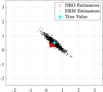
(a) $\rho=0.95$

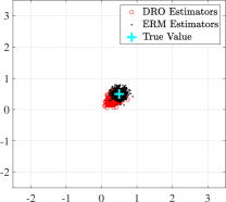
(b) $\rho=0$

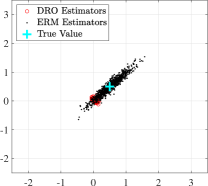
(c) $\rho=-0.95$

Figure 1: Scatter plots of ${\hat{\theta}_{n}^{\,\textnormal{erm}}}$ (black circles) and ${\hat{\theta}_{n}^{\,\textnormal{dro}}}$ (red circles) for $\theta_{\ast}=[0.5,0.5]^{\intercal}$.

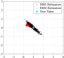
(a) $\rho=0.95$

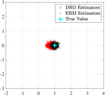
(b) $\rho=0$

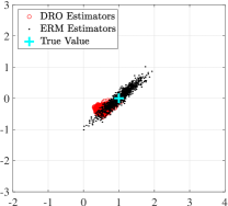
(c) $\rho=-0.95$

Figure 2: Scatter plots of ${\hat{\theta}_{n}^{\,\textnormal{erm}}}$ (black circles) and ${\hat{\theta}_{n}^{\,\textnormal{dro}}}$ (red circles) for $\theta_{\ast}=[1,0]^{\intercal}$.

Remark 2.8

Given the extensive coverage of the previous tutorial on Wasserstein DRO [51] and of other extensive surveys on DRO in general such as [73], we focus in this tutorial only on selected examples that we will use to connect to various statistical methodologies (including high-dimensional statistics and output analysis). However, DRO estimators have also been used in the context of non-parametric estimation (leading to the best known statistical rates) for instance, in the context of convex regression in which non-parametric functional regularization arises [9]. Other instances of regularization in the context of the 1-Wasserstein distance include support vector machines, norm-regularized logistic and quantile regression [78]. Shrinkage behaviors of statistical estimators can also be induced by the 2-Wasserstein DRO estimators; see, for example, [61]. At the other end of the spectrum, the $\infty$-Wasserstein distance can be used to formulate robust conditional expectation or quantile estimators [64] and tackle multistage problems [7].

3 Informing the ambiguity radius $\delta$ via Optimal Transport Projections

We next consider the question of selecting the ambiguity radius $\delta$ in (5) such that the resulting DRO formulation has desirable statistical properties. A possible approach towards this end is to select $\delta$ large enough so that the true data generating process belongs to a distributional ambiguity set with some prespecified confidence. This approach, which is often advocated in the literature in machine learning and robust control [79, 58, 66, 32, 96, 25, 21, 22, 17, 45, 16, 47], leads to a pessimistic selection of $\delta$ simply because this criterion is not informed at all by the loss function defining the decision problem. Indeed, the dimensional dependence in the the concentration inequalities used for this purpose is such that we will require an exponential amount in $m$ (the dimension of $X$) more samples to halve the error in the resulting DRO solution (see the discussion after Theorem 4.2 below).

Another approach involves the use of generalization bounds that are derived to obtain finite sample performance guarantees. While appealing, this method usually requires distributions with compact support or sub-Gaussian tail assumptions on the underlying distributions and some of these bounds, in turn, rely on the convergence rate of the empirical Wasserstein distance [34, 39]. Another complicating factor in their use is that the multiplicative constants involved in the bounds tend to be pessimistic or difficult to compute for the problem-in-hand.

The most popular approach used in practice is based on cross-validation (CV). Despite its popularity, CV is often used in a way which could lead to inconsistent estimation (i.e., the incorrect identification of the optimal decision). For example, holdout and leave-one-out CV does not guarantee consistency in multivariate regression estimation. The $k$-fold CV approach leads to consistent estimation, but it requires $k/n\rightarrow 1$ and $n-k\rightarrow\infty$ as $n\rightarrow\infty$ (see, for example, [81]). As a consequence, when applying $k$-fold cross validation one needs to solve $k$ optimization problems. Typically, $k$ is chosen as a small number such as $k=5$, but given the cautionary results in [81] it is unclear if these choices are always appropriate relative to a given sample size $n$.

In the specific context of the distributionally robust precision matrix estimation [61], the Wasserstein ambiguity size that minimizes the expected distance between the estimator and the true precision matrix scales linearly with the sample size as $n^{-1}$, where the proportionality constant is a function of the true covariance matrix that is known in closed form [15, Theorem 1]. The analysis in [15], however, depends on the analytical solution of the estimator and thus can only be generalized on a case-by-case basis.

Here we explain a generically applicable projection based statistical inference method called the Wasserstein Profile Function, introduced in [10], for optimally informing the ambiguity radius $\delta$ in (5). While the approach, as we shall see, enforces an optimality criterion at the level of decisions and not the value function, the methodology can be used to infer bounds on the optimal value as we shall discuss, see for example Theorem 4 in [10]. Intuitively, the Wasserstein Profile Function computes the projection, along with the corresponding distance, of the empirical distribution ${P}_{n}$ to a linear manifold of distributions which characterize the optimal decision. The use of these types of projection criteria to perform statistical inference is prevalent in statistics: [67] provides a comprehensive reference for projections, or profile functions, computed based on likelihood ratio metrics or the Kullback-Liebler divergence. The work of [54, 30, 52] connect these types of projections to DRO in the context of divergence measures.

Before giving the rationale behind the use of the Wasserstein Profile Function in the selection of $\delta$, we first develop an understanding of this projection based inference procedure in the elementary context of statistical hypothesis testing. The optimality of the prescription of $\delta$ and related statistical implications are explored in subsequent sections.

3.1 Statistical hypothesis testing with projection based profile inference.

Given independent samples $X_{1},\ldots,X_{n}$ from the unknown distribution $P_{\ast}$, we are interested in assessing if a given $\theta_{0}\in\Theta$ satisfies the equation $E_{{P}_{\ast}}[h(X,\theta_{0})]=0$. Towards this end, for each $\theta\in\Theta$, let

$$\mathcal{F}_{\theta}\coloneqq\left\{{P}\in\mathcal{P}(\mathcal{X}):E_{{P}}\left[h(X,\theta)\right]=0\right\}$$ (10)

denote the set of distributions of the random vector $X$ that satisfies the condition $E_{P}[h(X,\theta)]=0$. With this notation, our testing problem can be written as a statistical test with the hypotheses

$$\mathcal{H}_{0}:{P}_{\ast}\in\mathcal{F}_{\theta_{0}}\quad\text{ against }\quad\mathcal{H}_{1}:{P}_{\ast}\notin\mathcal{F}_{\theta_{0}}.$$

With the null hypothesis $\mathcal{H}_{0}$ stipulating the condition $E_{{P}_{\ast}}[h(X,\theta_{0})]=0$, the statistical test will detect the failure of the parameter choice $\theta_{0}$ in satisfying this condition with a pre-specified confidence. Equipped with the Wasserstein distance, testing the inclusion $P_{\ast}\in\mathcal{F}_{\theta_{0}}$ is equivalent to testing the distance from $P_{\ast}$ to the set $\mathcal{F}_{\theta_{0}}$ being zero. With this perspective, the hypotheses can be expressed as

$$\mathcal{H}_{0}:\inf_{P\in\mathcal{F}_{\theta_{0}}}D_{c}({P}_{\ast},P)=0\quad\text{ against }\quad\mathcal{H}_{1}:\inf_{P\in\mathcal{F}_{\theta_{0}}}D_{c}({P}_{\ast},P)>0.$$

To develop a suitable test statistic, we define the projection distance function of the empirical distribution ${P}_{n}=\frac{1}{n}\sum_{i=1}^{n}\delta_{X_{i}}$ onto $\mathcal{F}_{\theta}$ as

$$\mathcal{P}({P}_{n},\theta)\coloneqq\inf_{{P}\in\mathcal{F}_{\theta}}D_{c}({P}_{n},{P})=\left\{\begin{array}[]{cl}\inf&D_{c}({P}_{n},{P})\\ \mathrm{s.t.}&E_{{P}}\left[h(X,\theta)\right]=0.\end{array}\right.$$ (13)

We address the projection metric $\mathcal{P}(P_{n},\theta)$, viewed as a function of $\theta$, as the Wasserstein Profile Function. Equipped with the definition (13), the statistical test will proceed generically as follows: for a pre-specified significance level $\alpha\in(0,1)$,

reject $\mathcal{H}_{0}$ if $s_{n}>\eta_{{}_{1-\alpha}}$,

where $s_{n}$ is a test statistic that depends on the projection distance $\mathcal{P}(P_{n},\theta_{0})$, and $\eta_{{}_{1-\alpha}}$ is the $(1-\alpha)\times 100\%$ quantile of a limiting distribution obtained by studying the limit of $\mathcal{P}(P_{n},\theta_{0})$ as the number of samples $n$ tends to infinity. To operationalize this statistical test, we will now examine a dual reformulation of the projection distance $\mathcal{P}(P_{n},\theta_{0})$ and its limiting behavior as $n\rightarrow\infty$.

3.1.1 Dual reformulation for $\mathcal{P}(P_{n},\theta)$

Similar to the dual formulation of the worst-case risk $\mathcal{R}_{\delta}(P_{n},\theta)$ presented in Theorem 2.1, the projection distance $\mathcal{P}(P_{n},\theta)$ admits a dual reformulation due to the linear programming structure offered by the optimal transport costs. To state the dual reformulation, define $\tilde{\Theta}\subseteq\mathbb{R}^{d}$ as

$$\tilde{\Theta}\coloneqq\left\{\theta\in\Theta^{\circ}:0\in\textnormal{conv}\left[\{h(x,\theta):x\in\mathcal{X}\}\right]^{\circ}\right\},$$

where $\textnormal{conv}(S)$ denotes the convex hull of the set $S$, and $A^{\circ}$ indicates the interior of a set $A$. Since $\theta\notin\tilde{\Theta}$ cannot be a solution to $E_{{P}}[h(X,\theta)]=0$ unless ${P}$ is degenerate, it is sufficient to restrict the analysis to $\theta\in\tilde{\Theta}$.

Proposition 3.1 (Dual reformulation for $\mathcal{P}({P}_{n},\theta)$)

Let $h:\mathbb{R}^{m}\times\mathbb{R}^{d}\rightarrow\mathbb{R}^{k}$ be Borel measurable and $\{(x,x^{\prime})\in\mathcal{X}\times\mathcal{X}:c(x,x^{\prime})<+\infty\}$ be Borel measurable and nonempty. Then for any $\theta\in\tilde{\Theta}$,

$$\mathcal{P}({P}_{n},\theta)=-\sup_{\lambda\in\mathbb{R}^{k}}\frac{1}{n}\sum_{i=1}^{n}\sup_{x\in\mathcal{X}}\left\{\lambda^{\intercal}h(x,\theta)-c(X_{i},x)\right\}.$$

Verification of Proposition 3.1, as illustrated in [10, Appendix B], utilizes semi-infinite linear program duality. One may however quickly check the identity for the case where $\mathcal{X}$ is finite, as in the passage following Theorem 2.1.

3.1.2 The limiting behavior of $\mathcal{P}({P}_{n},\theta_{0})$ under $\mathcal{H}_{0}$

To see how we can obtain a test statistic from the projection $\mathcal{P}({P}_{n},\theta_{0})$, we next consider a suitably scaled version of $\mathcal{P}({P}_{n},\theta_{0})$ and obtain its limiting distribution when the data-generating ${P}_{\ast}\in\mathcal{F}_{\theta_{0}}$. Taking the special case $\mathcal{X}=\mathbb{R}^{m}$ and $c(x,x^{\prime})=\|x-x^{\prime}\|_{q}^{2}$, we rewrite the dual reformulation in Proposition 3.1 as

$$n\times\mathcal{P}({P}_{n},\theta_{0})$$

$$\qquad=\sup_{\lambda\in\mathbb{R}^{k}}\left\{n^{1/2}\lambda^{\intercal}H_{n}-\frac{1}{n}\sum_{i=1}^{n}\sup_{x\in\mathbb{R}^{m}}\left\{n\lambda^{\intercal}\big{[}h(X_{i}+n^{-1/2}\Delta,\theta_{0})-h(X_{i},\theta_{0})\big{]}-\|\Delta\|_{q}^{2}\right\}\right\}$$ (14)

$$\qquad\approx\sup_{\xi\in\mathbb{R}^{k}}\left\{\xi^{\intercal}H_{n}-\Phi_{n}(\xi,\theta_{0})\right\},$$

where

$$H_{n}\coloneqq n^{-1/2}\sum_{i=1}^{n}h(X_{i},\theta_{0})\quad\text{ and }\quad\Phi_{n}(\xi,\theta)\coloneqq\frac{1}{n}\sum_{i=1}^{n}\sup_{\Delta\in\mathbb{R}^{m}}\left\{\xi^{\intercal}D_{x}h(X_{i},\theta)\Delta-\|\Delta\|_{q}^{2}\right\},$$

and $D_{x}$ denotes the partial derivative with respect to the variable $x$. The latter expression is obtained by changing variables from $\lambda$ to $\xi=\lambda n^{1/2}$, the variable $x$ inside the respective supremum as in $x=X_{i}+n^{-1/2}\Delta$, and using a first-order approximation for the difference $h(X_{i}+n^{-1/2}\Delta,\theta_{0})-h(X_{i},\theta_{0})$. A precise treatment of this term using the fundamental theorem of calculus can be found in [10, Appendix A].

The most important part of the derivation is the intuition provided by the scaling. The re-scaling involving $n^{-1/2}\Delta$ indicates that the optimal projection involves an optimal transport displacement of order $O(n^{-1/2})$, which is consistent with the Central Limit Theorem, but at a local level (meaning for each $X_{i}$).

Next, due to a similar application of Hölder’s inequality as in Example 2.4, the suprema in the definition of $\Phi_{n}(\xi,\theta)$ can be simplified to result in $\Phi_{n}(\xi,\theta)=\frac{1}{4n}\sum_{i=1}^{n}\|\xi^{\intercal}D_{x}h(X_{i},\theta)\|_{p}^{2}$. For the sake of brevity, define

$$\varphi(\xi,\theta)\coloneqq\frac{1}{4}E_{{P}_{\ast}}\|\xi^{\intercal}D_{x}h(X_{i},\theta)\|_{p}^{2}\quad\text{ and }\quad\varphi^{\ast}(z,\theta)\coloneqq\sup_{\xi}~{}\{\xi^{\intercal}z-\varphi(\xi,\theta)\}.$$ (15)

Notice that $\varphi$ is a convex function in $\xi$, and $\varphi^{*}$ is the convex conjugate of $\varphi$ with respect to the $\xi$ component. Then as a consequence of the law of large numbers and uniform locally Lipschitz conditions we have

$$\Phi_{n}(\xi,\theta)\rightarrow\varphi(\xi,\theta)\quad\text{ as }n\rightarrow\infty$$

uniformly over compact subsets of $\xi\in\mathbb{R}^{k}$ and $\theta\in\Theta$. As a result,

$$n\times\mathcal{P}(P_{n},\theta_{0})=\varphi^{\ast}(H_{n},\theta_{0})(1+o(1))$$

as the number of samples $n\rightarrow\infty$. If $\theta_{0}$ indeed satisfies $E_{{P}^{\ast}}[h(X,\theta_{0})]=0$, then the sequence $\{H_{n}\}_{n\geq 1}$ converges in distribution (due to the Central Limit Theorem) and we obtain the limiting result as a consequence. In the following, we use $\overset{dist.}{\longrightarrow}$ to denote convergence in distribution.

Theorem 3.2 (Limit theorem for $\mathcal{P}({P}_{n},\theta)$)

Suppose the function $h(\cdot,\theta_{0})$ is continuously differentiable and $E_{{P}_{\ast}}[D_{x}h(X,\theta_{0})D_{x}h(X,\theta_{0})^{\intercal}]\succ 0$. Then under the null hypothesis $\mathcal{H}_{0}$,

$$n\times\mathcal{P}(P_{n},\theta_{0})\overset{dist.}{\longrightarrow}\varphi^{\ast}(H,\theta_{0})\quad\text{ as }n\rightarrow\infty,$$

where $H\sim\mathcal{N}(0,\mathrm{Cov}_{P_{\ast}}[h(X,\theta_{0})])$.

Remark 3.3

Recall that $c(x,x^{\prime})=\|x-x^{\prime}\|_{q}^{2}$, so in terms of the Wasserstein distance of order 2 (i.e., $r=2$) the projection converges to zero under the null hypothesis at rate $O(n^{-1/2})$. The proof of this result, along with extensions for the case $r\geq 1$, is given in [10] assuming that $(X_{1},...,X_{n})$ is an i.i.d. collection. As one can see from the discussion leading to Theorem 3.2, the key ingredients really are a functional law of large numbers for $\mathcal{P}(P_{n},\theta)$ over compact sets and a Central Limit Theorem for $H_{n}$, both of which hold well beyond the i.i.d. assumptions imposed here and in [10]. The work [8] discusses non-i.i.d. extensions which are relevant in financial applications, in particular, the mean-variance portfolio allocation problem.

Conceptually, Theorem 3.2 reveals that $s_{n}=n\times\mathcal{P}({P}_{n},\theta_{0})$ serves as a test statistic to reject the null hypothesis $\mathcal{H}_{0}$. In particular, for a pre-specified significance level $\alpha\in(0,1)$, let $\eta_{{}_{1-\alpha}}$ denote the $(1-\alpha)\times 100\%$ quantile of the limiting distribution given by the law of $\varphi^{\ast}(H,\theta_{0})$. Then rejecting $\mathcal{H}_{0}$ if $s_{n}>\eta_{{}_{1-\alpha}}$ results in a statistical test with Type-I error probability $\alpha$. The test distribution is determined by $\text{Cov}_{{P}_{\ast}}[h(X,\theta_{0})]$. The test distribution is unaffected by using any consistent plug-in estimator of the covariance matrix if it is unknown.

We now dive into an application of the proposed hypothesis test for fair classification [88].

Example 3.4 (Test for probabilistic fair classifier)

Consider the joint random vector $(X,A,Y)$ consisting of a feature vector $X\in{\mathbb{R}}^{d}$, a sensitive attribute $A\in\{0,1\}$ and a class label $Y\in\{0,1\}$. A logistic classifier aims to predict the class label $Y$ for any feature input $X$. A logistic classifier can be represented by the conditional distribution function $h_{\theta}$ of $Y$ given $X$ of the sigmoid form

$$h_{\theta}(x)=\frac{1}{1+\exp(-\theta^{\top}x)}.$$

Following the definition in [72], we say that a probabilistic classifier $h_{\theta}$ satisfies the probabilistic equal opportunity criterion relative to a distribution ${P}$ if

$$E_{{P}}[h_{\theta}(X)|A=1,Y=1]=E_{{P}}[h_{\theta}(X)|A=0,Y=1].$$

As a consequence, the manifold of distributions that renders $h_{\theta}$ a fair classifier is defined specifically as

$$\mathcal{F}_{\theta}=\left\{Q\in\mathcal{P}({\mathbb{R}}^{d}\times\{0,1\}\times\{0,1\}):E_{Q}[h_{\theta}(X)|A=1,Y=1]=E_{Q}[h_{\theta}(X)|A=0,Y=1]\right\}.$$

Suppose that $(X_{i},A_{i},Y_{i})$ are i.i.d. samples from $P_{\ast}$ and that the ground transport cost is of the form $c\big{(}(x^{\prime},a^{\prime},y^{\prime}),(x,a,y)\big{)}=\|x-x^{\prime}\|_{q}^{2}+\infty|a-a^{\prime}|+\infty|y-y^{\prime}|$. Under the null hypothesis $\mathcal{H}_{0}:~{}P_{\ast}\in\mathcal{F}_{\theta}$, we have the following limit distribution

$$n\times\mathcal{P}({P}_{n},\theta){\overset{dist.}{\longrightarrow}}\beta\chi_{1}^{2},$$

where $\chi_{1}^{2}$ is a chi-square distribution with 1 degree of freedom,

$$\beta=\left(E_{P_{\ast}}\left[\left\|\nabla h_{\theta}(X)\left(\frac{\mathbb{I}_{(1,1)}(A,Y)}{p_{11}}-\frac{\mathbb{I}_{(0,1)}(A,Y)}{p_{01}}\right)\right\|_{p}^{2}\right]\right)^{-1}\frac{\sigma^{2}}{p_{01}^{2}p_{11}^{2}}$$

with $\sigma^{2}=\mathrm{Cov}(Z)$, $p_{a1}={P}_{\ast}(A=a,Y=1)$, $\mathbb{I}$ is the indicator function and $Z$ is the univariate random variable

$$Z =h_{\theta}(X)\left(p_{01}\mathbb{I}_{(1,1)}(A,Y)-p_{11}\mathbb{I}_{(0,1)}(A,Y)\right)$$

$$\qquad+\mathbb{I}_{(0,1)}(A,Y)E_{P_{\ast}}[\mathbb{I}_{(1,1)}(A,Y)h_{\theta}(X)]-\mathbb{I}_{(1,1)}(A,Y)E_{P_{\ast}}[\mathbb{I}_{(0,1)}(A,Y)h_{\theta}(X)].$$

Given a logistic classifier parametrized by $\theta$, the decision to reject the probabilistic fairness of this classifier now relies on computing the projection distance $\mathcal{P}(P_{n},\theta)$ and on computing the empirical quantile estimate of $\beta\chi_{1}^{2}$ [88].

The limit result in Theorem 3.2 relies on the assumption that $h$ is continuously differentiable. The extension of the limiting distribution when $h$ is non-differentiable, or even when $h$ is discontinuous, can be found in [84]. The machinery of the Wasserstein Profile Function is also applied for model selection of graphical Lasso [24]. It is important to notice that the hypothesis testing framework outlined in this section is fundamentally different from the robust hypothesis test with Wasserstein ambiguity set proposed in [38]. Therein, the test is constructed to minimize the worst-case error, measured by the maximum of the type-I and type-II errors, uniformly over all perturbations of the empirical distribution in the ambiguity set.

The next section explains how this hypothesis testing procedure can guide us to choose the ambiguity radius $\delta$ optimally in a certain statistical sense.

3.2 Informing DRO ambiguity radius $\delta$ from the projection $\mathcal{P}(P_{n},\theta)$

Going back to the DRO formulation (4), assume $\ell(x,\cdot)$ is convex for every $x\in\mathcal{X}$ and let

$$h(x,\theta)\coloneqq D_{\theta}\ell(x,\theta)$$

denote the partial derivative of the loss function $\ell$. Fix an arbitrary distribution ${P}$ in the ambiguity set $\mathcal{U}_{\delta}({P}_{n})$ and suppose that $E_{{P}}[h(X,\theta)]=0$ specifies the necessary and sufficient condition for minimizing the risk $\mathcal{R}({P},\theta)$ over the feasible parameters $\theta\in\Theta$. In this case, the set $\{\theta\in\Theta:{P}\in\mathcal{F}_{\theta}\}$ (recall the definition of $\mathcal{F}_{\theta}$ in (10)) contains all parameter choices that are optimal from the decision maker’s point of view. Consequently, by taking unions over all $P\in\mathcal{U}_{\delta}({P}_{n})$, the set

$$\Lambda_{\delta}({P}_{n}) \coloneqq\left\{\theta\in\Theta:\mathcal{F}_{\theta}\cap\,\mathcal{U}_{\delta}({P}_{n})\neq\varnothing\right\}$$ (16)

$$=\left\{\theta\in\Theta:\mathcal{R}({P},\theta)=\mathcal{R}_{\ast}({P})\right\}$$

includes all the parameter choices that are collected by the decision maker as optimal for some distribution in the distributional uncertainty set $\mathcal{U}_{\delta}({P}_{n})$. This leads to the following notion of compatible confidence regions.

3.2.1 Confidence regions compatible with the DRO formulation (4).

If $\mathcal{U}_{\delta}({P}_{n})$ represents a family of plausible representations of uncertainty around $P_{n}$, then $\Lambda_{\delta}({P}_{n})$ in (16) represents a family of plausible decisions. One can therefore think of $\Lambda_{\delta}({P}_{n})$ as the projection of $\mathcal{U}_{\delta}({P}_{n})$ onto the decision space (which is finite-dimensional and informed by the optimization problem of interest). In that sense, one can view $\Lambda_{\delta}({P}_{n})$ as a set of decisions $\theta\in\Theta$ that are compatible with the distributional uncertainty $\mathcal{U}_{\delta}({P}_{n}).$ If we can guarantee that the set $\Lambda_{\delta}({P}_{n})$ contains an optimal $\theta_{\ast}$ solving (1) with probability $1-\alpha,$ then $\Lambda_{\delta}({P}_{n})$ becomes a compatible confidence region for a correct decision for the problem (1).

Since the family of sets $\{\Lambda_{\delta}({P}_{n}):\delta>0\}$ is increasing in $\delta$ it is clear that a minimizer of (1) will be a member of $\Lambda_{\delta}({P}_{n})$ for a sufficiently large choice of $\delta$. Indeed, this holds true when ${P}_{\ast}\in\mathcal{U}_{\delta}({P}_{n})$, or more explicitly, when $\delta$ is chosen such that $D_{c}({P}_{n},{P}_{\ast})\leq\delta$. Based on these considerations, since solving (1) is our primary objective, this leads to the following natural enquiry:

In other words, we seek to identify

$$\delta_{\ast}\coloneqq\inf\big{\{}\delta>0:\Lambda_{\delta}({P}_{n})\text{ contains a minimizer of \eqref{prm} with }(1-\alpha)\text{-confidence}\big{\}}.$$ (17)

The desire to identify the smallest $\delta$ (satisfying this criterion) is motivated by the need to drive down the conservativeness of the resulting DRO formulation (4).

3.2.2 Identifying the optimal radius $\delta_{\ast}$ from the projection profile $\mathcal{P}({P}_{n},\theta).$

The above question leads to a data-driven choice of the ambiguity size $\delta$ that is explicitly linked to the statistician’s decision problem and can be answered with the projection-based profile function $\mathcal{{P}}({P}_{n},\theta)$ introduced in Section 3.1 for testing the hypothesis ${P}_{\ast}\in\mathcal{F}_{\theta}$. To see the link between these apparently different exercises, suppose that any solution $\theta_{\ast}\in\text{arg}\,\text{min}_{\theta\in\Theta}E_{{P}_{\ast}}\left[\ell(X,\theta)\right]$ satisfies the optimality condition

$$E_{{P}_{\ast}}\left[h(X,\theta_{\ast})\right]=0.$$

Then the minimal radius $\delta_{\ast}$ in (17) can be re-expressed as

$$\delta_{\ast} =\inf\left\{\delta>0:\exists\theta\in\Lambda_{\delta}({P}_{n})\text{ such that }{P}_{\ast}\in\mathcal{F}_{\theta}\text{ with }(1-\alpha)\text{-confidence}\right\}$$

$$\overset{(a)}{=}\inf\left\{\delta>0:\exists({P},\theta)\in\mathcal{U}_{\delta}({P}_{n})\times\Theta\text{ such that }{P}\in\mathcal{F}_{\theta},{P}_{\ast}\in\mathcal{F}_{\theta}\text{ with }(1-\alpha)\text{-confidence}\right\}$$

$$\overset{(b)}{=}\inf\left\{\delta>0:\exists\theta\in\Theta\text{ such that }\mathcal{P}({P}_{n},\theta)\leq\delta,\ {P}_{\ast}\in\mathcal{F}_{\theta}\text{ with }(1-\alpha)\text{-confidence}\right\}$$

$$\overset{(c)}{=}\inf\left\{\delta>0:\exists\theta\in\Theta\text{ such that }\mathcal{P}({P}_{n},\theta)\leq\delta,\ n\mathcal{P}({P}_{n},\theta)\leq\eta_{{}_{1-\alpha}}(1+o(1))\right\}$$

$$=n^{-1}\times\eta_{{}_{1-\alpha}}(1+o(1)),$$

where (a) and (b) follow respectively from the definitions of $\Lambda_{\delta}({P}_{n})$ and of $\mathcal{P}({P}_{n},\theta)$, (c) from the statistical test developed in Section 3.1 for rejecting the null hypothesis $\mathcal{H}_{0}:{P}_{\ast}\in\mathcal{F}_{\theta}$ with $(1-\alpha)$-confidence, and the last equality holds if a solution $\theta_{\ast}$ to (1) satisfying ${P}_{\ast}\in\mathcal{F}_{\theta_{\ast}}$ exists.

Thus, instead of requiring $\delta>0$ to be large enough such that the data-generating ${P}_{\ast}\in\mathcal{U}_{\delta}({P}_{n})$, the projection based prescription merely requires existence of ${P}\in\mathcal{U}_{\delta}$ such that ${P}\in\mathcal{F}_{\theta}$ for some population risk minimizer $\theta_{\ast}\in\Theta$. While this choice results in $\delta\propto n^{-1}$ and the guarantee that $\Lambda_{\delta}({P}_{n})$ serves as a confidence region for the solutions to (1), the former prescription from concentration inequalities results in a pessimistic $\delta\propto n^{-2/m}$ under additionally restrictive assumptions, where $m$ is the ambient dimension of the space ${\mathcal{X}}$ in which the random vector $X$ takes values (see, for example, [93, 27, 31, 51]).

Algorithm 1 below provides a recipe for estimating $\delta$ in order to guarantee asymptotic optimality in the sense of ensuring the smallest choice which guarantees $1-\alpha$ coverage.

Algorithm 1 A recipe for DRO estimation (4) with optimal selection of the ambiguity radius $\delta$.

  Input: Training samples $X_{1},\ldots,X_{n}$ from an unknown distribution ${P}_{\ast}$.

  Outline of steps:

  1. Let $\hat{\Sigma}$ be the sample covariance of $\{h(X_{1},{\hat{\theta}_{n}^{\,\textnormal{erm}}}),\ldots,h(X_{n},{\hat{\theta}_{n}^{\,\textnormal{erm}}})\}$, where $h(X,\theta)=D_{\theta}\ell(X,\theta)$ and ${\hat{\theta}_{n}^{\,\textnormal{erm}}}\in\argmin_{\theta\in\Theta}~{}{E}_{{P}_{n}}[\ell(X,\theta)]$.

  2. Obtain independent samples $H_{1},\ldots,H_{k}$ from $\mathcal{N}(0,\hat{\Sigma})$. (Any choice of $k$ such that $k\rightarrow\infty$ as $n\rightarrow\infty$ is valid, for example, $k=\log(n)$.) Let $\hat{\eta}_{1-\alpha}$ be the $(1-\alpha)$-quantile of the sample collection $\{\hat{\varphi}^{\ast}(H_{i},{\hat{\theta}_{n}^{\,\textnormal{erm}}}):i=1,\ldots,k\}$, where $\hat{\varphi}^{\ast}$ is the convex conjugate of $\hat{\varphi}(\cdot)$ in (22). In the absence of the knowledge of the conjugate $\hat{\varphi}^{\ast}$, one may take $\hat{\eta}_{1-\alpha}$ of a tractable upper bound of $\varphi^{\ast}(\cdot)$, as illustrated in Example 3.6.

  3. Let ${\hat{\theta}_{n}^{\,\textnormal{dro}}}\in\argmin_{\theta\in\Theta}~{}{\mathcal{R}_{\delta}}({P}_{n},\theta)$ be a solution to the DRO estimation (4) obtained by letting $\delta=n^{-1}\times\eta_{1-\alpha}$.

  4. Return ${\hat{\theta}_{n}^{\,\textnormal{dro}}}$ as the distributionally robust solution.

3.2.3 Illustrative examples.

We illustrate the choice of $\delta$ prescribed in Algorithm 1 via some illustrative examples.

Example 3.5 (Identifying the radius $\delta=n^{-1}\eta_{1-\alpha}$ for linear regression example)

Continuing the discussion in Example 2, we see that $h(x,y,\theta)=D_{\theta}\ell(x,y,\theta)=(y-\theta^{\intercal}x)x$. Consider the linear regression model

$$Y=\theta_{\ast}^{\intercal}X+e,$$ (18)

where the unknown $\theta_{\ast}\in\mathbb{R}^{d}$ and the independent additive error $e$ has zero mean and variance $\sigma^{2}$. Letting ${P}_{\ast}$ be the distribution of $(X,Y)$, we have $E_{{P}_{\ast}}[h(X,Y,\theta_{\ast})]=E_{{P}_{\ast}}[eX]=0$. Then under the null hypothesis $\mathcal{H}_{0}:{P}_{\ast}\in\mathcal{F}_{\theta_{\ast}}$, we have from Theorem 3.2 that $n\mathcal{P}({P}_{n},\theta_{\ast})\overset{dist.}{\longrightarrow}\varphi^{\ast}(H,\theta_{\ast})$, where $H\sim\mathcal{N}(0,\sigma^{2}\Xi)$, $\Xi=E_{P_{\ast}}[XX^{\intercal}]$ and

$$\varphi^{\ast}(z,\theta_{\ast}) =\sup_{\xi}\left\{\xi^{\intercal}z-4^{-1}E_{{P}_{\ast}}\left\|e\xi-\xi^{\intercal}X\theta_{\ast}\right\|_{p}^{2}\right\}.$$

Taking $q=2$ in the transportation cost in (8) for ease of illustration, we see that

$$\varphi^{\ast}(z,\theta_{\ast}) =\sup_{\xi}\left\{\xi^{\intercal}z-4^{-1}\xi^{\intercal}\left(\sigma^{2}\mathbb{I}_{d}+\Xi\|\theta_{\ast}\|_{2}^{2}\right)\xi\right\}$$

$$=z^{\intercal}\left(\sigma^{2}\mathbb{I}_{d}+\Xi\|\theta_{\ast}\|_{2}^{2}\right)^{-1}z.$$

The limit $\varphi^{\ast}(H,\theta_{\ast})$ has a generalized chi-square distribution in this case. If ${E}_{{P}_{\ast}}[X]=0$ and $\Xi$ is invertible with eigen decomposition $\Xi=UDU^{\intercal}$, then we have that $N=D^{-1/2}U^{\intercal}H$ is a standard normal vector with mean 0 and covariance $\mathbb{I}_{d}$. As a result,

$$\varphi^{\ast}(H,\theta_{\ast})=\sum_{i=1}^{d}\frac{D_{ii}}{1+D_{ii}\|\theta_{\ast}\|_{2}^{2}/\sigma^{2}}N_{i}^{2},$$

where $D_{ii}$ is the $i$-th diagonal element of the matrix $D$. One may compute an estimate of the quantile $\hat{\eta}_{{}_{1-\alpha}}$ by plugging in any consistent estimators for $\theta_{\ast}$ and $\Xi$. The asymptotic validity of $\delta$ in terms of coverage and hypothesis testing remains unchanged by plugging in consistent estimators in this case because the limiting distribution function is continuous as a function of these parameters.

Example 3.6 (A prescription for $\delta$ in high-dimensional linear regression)

We now consider the linear regression model (18) in the high-dimensional setting where $d\gg n$. Choosing the transportation cost $c$ in (8) with $q=a=\infty$, the resulting DRO linear regression problem coincides with the square-root Lasso estimator in [4]. We now examine the prescription $\delta=n^{-1}\eta_{{}_{1-\alpha}}$ arising from the projection metric $\mathcal{P}({P}_{n},\theta)$. Since $d\rightarrow\infty$ as $n\rightarrow\infty$, the limiting characterization in Theorem 3.2 does not hold and therefore we take $\eta_{{}_{1-\alpha}}$ directly to be the $(1-\alpha)$-quantile of the pre-limit $n\mathcal{P}({P}_{n},\theta_{\ast})$. Resorting to (14) for this purpose, we see that $n\mathcal{P}({P}_{n},\theta_{\ast})$ is merely the convex conjugate of

$$\tilde{\Phi}_{n}(\xi) =\frac{1}{n}\sum_{i=1}^{n}\sup_{\Delta}\left\{n^{1/2}\xi^{\intercal}[Y_{i}-\theta_{\ast}^{\intercal}(X_{i}+n^{-1/2}\Delta)(X_{i}+n^{-1/2}\Delta)]-\|\Delta\|_{\infty}^{2}\right\}$$

$$=\frac{1}{n}\sum_{i=1}^{n}\sup_{\Delta}\left\{e_{i}\xi^{\intercal}\Delta-(\theta_{\ast}^{\intercal}\Delta)(\xi^{\intercal}X_{i})-\left[1+n^{-1/2}\frac{(\theta_{\ast}^{\intercal}\Delta)(\xi^{\intercal}\Delta)}{\|\Delta\|_{\infty}^{2}}\right]\|\Delta\|_{\infty}^{2}\right\},$$

evaluated at $H_{n}=n^{-1/2}\sum_{i=1}^{n}e_{i}X_{i}$. Bounding the inner-products involving $\Delta$ using Hölder’s inequality results in the following nonasymptotic bound for the inner suprema:

$$\tilde{\Phi}_{n}(\xi)\geq\Phi_{n}(\xi)\coloneqq\frac{1}{n}\sum_{i=1}^{n}\frac{\|e_{i}\xi-(\xi^{\intercal}X_{i})\theta_{\ast}\|_{1}^{2}}{1+n^{-1/2}\|\theta_{\ast}\|_{1}\|\xi\|_{1}}.$$

The convex conjugate of $\tilde{\Phi}_{n}(\cdot)$, denoted by $\Phi_{n}^{\ast}(\cdot)$, can be bounded as $\Phi_{n}^{\ast}(z)\leq\|z\|_{\infty}^{2}/\text{Var}_{n}|e|$ $(1+o(1))$. Here $\text{Var}_{n}|e|$ is the sample variance of the collection $\{|e_{i}|\}_{i=1}^{n}$. The intermediate steps involved in arriving at the upper bound of the convex conjugate is available in the proof of Theorem 7 in [10]. Since $n\mathcal{P}({P}_{n},\theta_{\ast})=\sup_{\xi}\{\xi^{\intercal}H_{n}-\tilde{\Phi}_{n}(\xi)\}$, the following upper bound for $n\mathcal{P}({P}_{n},\theta_{\ast})$ can be obtained from an upper bound for the convex conjugate of $\Phi_{n}(\cdot):$

$$n\mathcal{P}({P}_{n},\theta_{\ast})\leq\frac{\|H_{n}\|_{\infty}^{2}}{\text{Var}_{n}|e|}(1+o(1)),$$

as $n\rightarrow\infty$. Suppose that the additive noise $e$ is normally distributed and the observations $X_{i}=(X_{i1},...,X_{id})$ are normalized so that $n^{-1}\sum_{i=1}^{n}X_{ij}^{2}=1$, for $j=1,\ldots,d$. Then for any $\alpha<1/8,C>0,\varepsilon>0$, one can conclude the following from [4, Lemma 1(iii)]: Conditional on the observations $\{X_{i}:i=1,...,n\}$,

$$n\times\mathcal{P}({P}_{n},\theta_{\ast})\leq\eta_{{}_{1-\alpha}}\coloneqq\left[\frac{\pi}{\pi-2}\Phi^{-1}(1-\alpha/2d)\right]^{2},$$

with probability larger than $1-\alpha$, as $n\rightarrow\infty$, uniformly in $d$ such that $\log d\leq Cn^{1/2-\varepsilon}$. Here $\Phi^{-1}(1-\alpha)$ denotes the $(1-\alpha)$-quantile of the standard normal random variable. This results in the choice of ambiguity radius $\delta=n^{-1}\times\eta_{{}_{1-\alpha}}$. The respective regularization parameter in (9) is given by

$$\delta_{n}^{1/2}=n^{-1/2}\times\frac{\pi}{\pi-2}\Phi^{-1}(1-\alpha/2d),$$

which agrees with the prescription obtained independently in the statistics literature for recovering $\theta_{\ast}$ in high-dimensional settings when $d\gg n$; see, for example, [4, Corollary 1]. Another interesting aspect of this choice is its self-normalizing property that renders the selection independent of the error variance $\sigma^{2}$.

4 Statistical properties of DRO estimators and the optimality of $\delta=n^{-1}\eta_{{}_{1-\alpha}}$

For ease of illustrating the key ideas, we make the following simplifying assumptions throughout this section. A precise statement of results in more general settings can be found in the accompanying references.

The transportation cost $c(x,x^{\prime})=\|x-x^{\prime}\|_{q}^{2}$ for some $q\in(1,\infty]$.

The loss $\ell:\mathbb{R}^{m}\times\Theta\rightarrow\mathbb{R}$ is twice continuously differentiable with uniformly bounded second derivatives. For any $\theta\in\Theta$, $\{\ell(X,\theta):\theta\in\Theta\}$ has finite second moments.

4.1 Adaptive regularization induced by Wasserstein DRO formulations

We begin our analysis of the DRO estimation problem (4) with the series expansion of the DRO objective $\mathcal{R}_{\delta}({P}_{n},\theta)$ in Theorem 4.1 below. For $p$, $q$ satisfying $1/p+1/q=1$, let

$$\mathcal{V}^{2}_{p}({P},\theta)\coloneqq E_{{P}}\|D_{x}\ell(X,\theta)\|_{p}^{2}$$ (19)

denote the expected ‘squared variation’ in the loss or, in other words, the expected squared sensitivity of loss with respect to perturbations in the random vector $X$. Theorem 4.1 below asserts that the DRO estimation procedure (4) favours solutions which possess low sensitivity to perturbations, measured in terms of the regularizer $\mathcal{V}({P}_{n},\theta)$.

Theorem 4.1 (Variation regularization)

Under Assumptions 4 - 4, we have

$$\mathcal{R}_{\delta}({P}_{n},\theta)=E_{{P}_{n}}\left[\ell(X,\theta)\right]+\delta^{1/2}\mathcal{V}_{p}({P}_{n},\theta)+O_{p}(\delta),$$

for any choice of $\delta\rightarrow 0$ as $n\rightarrow\infty$. The convergence is uniform over $\theta$ in compact subsets of $\Theta$.

A precise characterization of the second-order error term, introduced by carefully incorporating the second-order terms in the Taylor expansion of $\ell$, is available in [13, Appendix A1]. A general version of the result, applicable for $c(x,x^{\prime})=\|x-x^{\prime}\|_{q}^{r}$ (with $r$ is not necessarily required to equal 2), is available in [37]. The limiting analysis in [13, 2] also characterizes the sensitivities of the optimizer as the radius of the Wasserstein ball is shrunk to zero.

For small values of the ambiguity radius $\delta$, Theorem 4.1 asserts that the DRO objective $\mathcal{R}_{\delta}({P}_{n},\theta)$ can be understood in terms of the empirical risk $\mathcal{R}({P}_{n},\theta)$ and a regularization term $\mathcal{V}({P}_{n},\theta)$ capturing the variation/sensitivity induced by the choice $\theta$. This connection with the empirical risk minimization objective allows the following interpretation: If there are several solutions with small empirical risk (which happens often in high-dimensional settings), the DRO estimation procedure (4) can be understood as favouring solutions which possess low sensitivity to perturbations, measured in terms of the regularizer $\mathcal{V}({P}_{n},\theta)$.

The conclusion in Corollary 2.2 serves as a good starting point to see why the expansion in Theorem 4.1 is plausible. Changing variables from $\lambda\delta^{1/2}$ to $\lambda$ and $\delta^{1/2}\Delta$ to $\Delta$ in the conclusion in Corollary 2.2,

$$\mathcal{R}_{\delta}({P}_{n},\theta)=\inf_{\lambda\geq 0}~{}\lambda\delta^{1/2}+\frac{1}{n}\sum_{i=1}^{n}\sup_{\Delta}\left\{\ell(X_{i}+\delta^{1/2}\Delta,\theta)-\lambda\delta^{1/2}\|\Delta\|_{q}^{2}\right\}.$$

Replacing the terms $\ell(X_{i}+\delta^{1/2}\Delta,\theta)$ by their respective first-order Taylor approximation, the inner suprema evaluate to

$$\sup_{\Delta}\left\{\ell(X_{i},\theta)+\delta^{1/2}D_{x}\ell(X_{i},\theta)^{\intercal}\Delta-\lambda\delta^{1/2}\|\Delta\|_{q}^{2}\right\}=\ell(X_{i},\theta)+\frac{\delta^{1/2}}{4\lambda}\|D_{x}\ell(X_{i},\theta)\|_{p}^{2}.$$

This leads to

$$\mathcal{R}_{\delta}({P}_{n},\theta) \approx E_{{P}_{n}}[\ell(X_{i},\theta)]+\delta^{1/2}\inf_{\lambda>0}~{}\left\{\lambda+\frac{E_{{P}_{n}}\|D_{x}\ell(X_{i},\theta)\|_{p}^{2}}{4\lambda}\right\}$$

$$=E_{{P}_{n}}[\ell(X_{i},\theta)]+\delta^{1/2}\mathcal{V}_{p}({P}_{n},\theta),$$

which heuristically justifies the conclusion in Theorem 4.1.

Unlike the exact regularization terms exhibited in specific instances in Examples 2.4 and 2, the asymptotic regularizing effect exhibited in Theorem 4.1 holds more broadly. More interesting is the observation that the regularization is adapted to the model informed by the loss $\ell$, such that the resulting sensitivity to perturbations in samples is small. Regularization terms involving this flavour have emerged useful in adversarial training in machine learning (see, for example, [44, 80, 92, 76]). A principled approach towards guaranteeing adversarial robustness in machine learning contexts using Wasserstein DRO solutions has been considered in [85].

4.2 Limiting behavior of the DRO estimator

The most common approach towards examining the statistical properties of an estimator is to study its limiting behavior as the number of samples grows to infinity. While based on our discussion in the previous section we know that $\gamma=1$ should be considered, here we examine the joint limiting behavior of the triplet

$$\big{(}\hat{\theta}_{n}^{\,\textnormal{erm}},\hat{\theta}_{n}^{\,\textnormal{dro}},\Lambda_{\delta}({P}_{n})\big{)}$$

for arbitrary $\gamma$. We must keep in mind that $\delta$ depends on $n$ but we omit this dependence to simplify the notation. While $\hat{\theta}_{n}^{\,\textnormal{erm}},\hat{\theta}_{n}^{\,\textnormal{dro}}$ are $\mathbb{R}^{d}$-valued, the third component in the triplet, namely, $\Lambda_{\delta}({P}_{n})\subseteq\mathbb{R}^{d}$, is the collection of optimizers compatible with the distributional ambiguity $\mathcal{U}_{\delta}({P}_{n})$. The limiting behavior of $\Lambda_{\delta}({P}_{n})$ will help us reinforce the optimality of the projection-based prescription $\delta=n^{-1}\times\eta_{{}_{1-\alpha}}$ and the construction of DRO-based confidence regions that are useful from the viewpoint of uncertainty quantification. To utilize the well-known machinery of set convergence (see, for example, [75, 59]) for this purpose, we consider the right-continuous version of $\Lambda_{\delta}({P}_{n})$, namely,

$$\Lambda_{\delta}^{+}({P}_{n})=\text{cl}\left(\cap_{\varepsilon>0}\Lambda_{\delta+\varepsilon}({P}_{n})\right),$$

that contains the compatible $\Lambda_{\delta}({P}_{n})$ and remains closed. We undertake this study of the limiting behavior assuming the existence of a unique minimizer $\theta_{\ast}$ for (1), as indicated in Assumption 4.2 below.

For each $x\in\mathbb{R}^{m}$, $\ell(x,\cdot)$ is convex. Letting $h(x,\theta)=D_{\theta}\ell(x,\theta)$, there exists $\theta_{\ast}\in\Theta^{\circ}$ satisfying the optimality conditions $E_{{P}_{\ast}}[h(X,\theta)]=0$, and $C\coloneqq E_{{P}_{\ast}}[D_{\theta}h(X,\theta_{\ast})]\succ 0$.

For $c>0$, define

$$b_{c}\coloneqq c^{1/2}C^{-1}D_{\theta}\mathcal{V}({P}_{\ast},\theta_{\ast})\quad\text{ and }\quad\Lambda_{c}\coloneqq\left\{u:\varphi^{\ast}(Cu,\theta_{\ast})\leq c\right\},$$

where $D_{\theta}$ is the derivative operator with respect to the parameter $\theta$. Ultimately, the following result will lead us to the optimal choice $c_{\ast}=\eta_{{}_{1-\alpha}}$.

Theorem 4.2 (Limit behavior)

Suppose that Assumptions 4 - 4.2 hold and the distribution ${P}_{\ast}$ is non-degenerate in the sense that ${P}_{\ast}(D_{x}\ell(X,\theta_{\ast})\neq 0)>0$ and that $E_{{P}_{\ast}}[D_{x}h(X,\theta_{\ast})D_{x}h(X,\theta_{\ast})^{\intercal}]\succ 0$. Let $Z=C^{-1}H$, where $H\sim\mathcal{N}(0,\Sigma)$ with covariance matrix $\Sigma\coloneqq\mathrm{Cov}_{{P}_{\ast}}[h(X,\theta_{\ast})]$. Then as $n\rightarrow\infty$, we have

• for $\delta=cn^{-1}$,

  $$\left(n^{1/2}[\hat{\theta}_{n}^{\,\textnormal{erm}}-\theta_{\ast}],\ n^{1/2}[\hat{\theta}_{n}^{\,\textnormal{dro}}-\theta_{\ast}],\ n^{1/2}[\Lambda_{\delta}^{+}({P}_{n})-\hat{\theta}_{n}^{\,\textnormal{erm}}]\right)\overset{dist.}{\longrightarrow}\big{(}Z,\ Z-b_{c},\ \Lambda_{c}\big{)};$$

• for $\delta=cn^{-\gamma}$ with $\gamma<1$,

  $$\left(n^{1/2}[\hat{\theta}_{n}^{\,\textnormal{erm}}-\theta_{\ast}],\ n^{\gamma/2}[\hat{\theta}_{n}^{\,\textnormal{dro}}-\theta_{\ast}],\ n^{1/2}[\Lambda_{\delta}^{+}({P}_{n})-\hat{\theta}_{n}^{\,\textnormal{erm}}]\right)\overset{dist.}{\longrightarrow}\big{(}Z,\ Z-b_{c},\ \mathbb{R}^{d}\big{)};$$

• and for $\delta=cn^{-\gamma}$ with $\gamma>1$,

  $$\left(n^{1/2}[\hat{\theta}_{n}^{\,\textnormal{erm}}-\theta_{\ast}],\ n^{1/2}[\hat{\theta}_{n}^{\,\textnormal{dro}}-\theta_{\ast}],\ n^{1/2}[\Lambda_{\delta}^{+}({P}_{n})-\hat{\theta}_{n}^{\,\textnormal{erm}}]\right)\overset{dist.}{\longrightarrow}\big{(}Z,\ Z,\ \{0\}\big{)}.$$

A proof of Theorem 4.2 is available in [13]. We focus on understanding its implications. The case where the radius of the Wasserstein ball is shrunk slower than the recommended rate $\delta\propto n^{-1}$ (the case where $\gamma<1$) results in

$$\|\hat{\theta}_{n}^{\,\textnormal{dro}}-\theta_{\ast}\|=O_{p}(n^{-\gamma/2}),$$

which is suboptimal in the large-sample regime, when compared with the benchmark set by empirical risk minimization. The rate is grossly inferior for the choice $\delta\propto n^{-2/d}$, recommended by the use of concentration inequalities. This characterization verifies the earlier assertion that halving the estimation error in the DRO solution will require $2^{d}$ more samples. The accompanying compatible optimal solution set $\Lambda_{\delta}^{+}({P}_{n})\approx\hat{\theta}_{n}^{\,\textnormal{erm}}+n^{-1/2}\mathbb{R}^{d}$, while including the true optimum $\theta_{\ast},$ is too large to be useful in any meaningful way.

When the radius of the Wasserstein ball is shrunk at the recommended $\delta\propto n^{-1}$, the characterization that

$$\hat{\theta}_{n}^{\,\textnormal{dro}} =\theta_{\ast}+n^{-1/2}(Z-b_{c})+o_{p}(n^{-1/2})$$

$$=\hat{\theta}_{n}^{\,\textnormal{erm}}-n^{-1/2}c^{1/2}C^{-1}D_{\theta}\mathcal{V}({P}_{n},\hat{\theta}_{n}^{\,\textnormal{erm}})+o_{p}(n^{-1/2}),$$

indicates the presence of an additional bias term $b_{c}=c^{1/2}C^{-1}D_{\theta}\mathcal{V}({P}_{\ast},\theta_{\ast})$. Since $\mathcal{V}(\cdot)$ in (19) can be understood as the measure of variation (or) sensitivity in the loss with respect to perturbations to realizations of $X$, the effect of the bias term can be understood as a “nudge” towards favouring solutions with lower sensitivity or variation measured by $\mathcal{V}({P}_{\ast},\theta)$. This is in line with the adaptive regularization interpretation developed in Section 4.1 for the DRO estimation (4).

On the other hand, for the case where the radius is shrunk faster than the recommended rate (that is, when $\gamma>1$),

$$\hat{\theta}_{n}^{\,\textnormal{dro}}=\hat{\theta}_{n}^{\,\textnormal{erm}}+o_{p}(n^{-1/2})\quad\text{ and }\quad\Lambda_{\delta}^{+}({P}_{n})=\{\hat{\theta}_{n}^{\,\textnormal{erm}}\}+o_{p}(n^{-1/2}),$$

revealing that there is no appreciable effect seen both in the DRO estimator $\hat{\theta}_{n}^{\,\textnormal{dro}}$ and the compatible set of optimal solutions.

While the above discussion justifies the rate of shrinking in $\delta=cn^{-1}$, for some $c>0$, the optimality of the particular prescription $c=\eta_{{}_{1-\alpha}}$ can be inferred from the limiting characterization as follows. Fix $\delta=cn^{-1}$. Then $\hat{\theta}_{n}^{\,\textnormal{erm}}-\theta_{\ast}=Z+o_{p}(n^{-1/2})$ and

$$\Lambda_{\delta}^{+}({P}_{n}) =\hat{\theta}_{n}^{\,\textnormal{erm}}+\Lambda_{c}+o_{p}(n^{-1/2})$$

$$=\theta_{\ast}+\{u+Z:\varphi^{\ast}(Cu,\theta_{\ast})\leq c\}+o_{p}(n^{-1/2}).$$

Therefore,

$$\theta_{\ast}\in\Lambda_{\delta}^{+}({P}_{n})\quad\text{ if and only if }\quad 0\in\left\{u:\varphi^{\ast}(C(u-Z),\theta_{\ast})\leq c\right\}+o_{p}(n^{-1/2}).$$

The optimal choice which ensures $\Lambda_{\delta}^{+}({P}_{n})$ is a $(1-\alpha)$-confidence region of $\theta_{\ast}$ is then given by,

$$c_{\ast} =\inf\{c>0:\theta_{\ast}\in\Lambda_{\delta}^{+}({P}_{n})\text{ with confidence }1-\alpha\}$$

$$=\inf\{c>0:\text{Pr}(\varphi^{\ast}(-CZ,\theta_{\ast})\leq c)\geq 1-\alpha\}$$

$$=\eta_{{}_{1-\alpha}},$$

since $\eta_{{}_{1-\alpha}}$ is defined in Section 3 as the $(1-\alpha)$-quantile of the limiting variable $\varphi^{\ast}(H,\theta_{\ast})$ and Law($H$) = Law($-CZ$).

4.3 Construction of DRO-compatible Confidence Regions.

To study the confidence regions for the purposes of uncertainty quantification, we further pursue the notion of compatible confidence regions introduced in Section 3.2.1. Recall that the set $\Lambda_{\delta}({P}_{n})$ serves as a projection of the distributional uncertainty $\mathcal{U}_{\delta}({P}_{n})$ onto the decision space and hence can be thought of as a confidence region compatible with the DRO formulation (4) when suitable statistical coverage is satisfied.

We begin this study with a Nash equilibrium characterization of the DRO estimator ${\hat{\theta}_{n}^{\,\textnormal{dro}}}.$ This can be achieved thanks to the following Theorem 4.3.

Theorem 4.3 (Inf-Sup interchange and Nash equilibrium)

Under Assumptions 4 and 4.2, we have

$$\inf_{\theta\in\Theta}\sup_{{P}\in\mathcal{U}_{\delta}({P}_{n})}E_{{P}}\left[\ell(X,\theta)\right]=\sup_{{P}\in\mathcal{U}_{\delta}({P}_{n})}\inf_{\theta\in\Theta}E_{{P}}\left[\ell(X,\theta)\right]$$

for any $\delta>0$. Further, there exists a distributionally robust optimal choice $\hat{\theta}_{n}^{\,\textnormal{dro}}\in\Lambda_{\delta}({P}_{n})$ and for a given $\varepsilon>0$, there exists a measure ${P}^{\ast}_{\varepsilon}\in\mathcal{U}_{\delta}({P}_{n})$ such that

$$\mathcal{R}({P},\hat{\theta}_{n}^{\,\textnormal{dro}})-\varepsilon\leq\mathcal{R}({P}^{\ast}_{\varepsilon},\hat{\theta}_{n}^{\,\textnormal{dro}})\leq\mathcal{R}({P}^{\ast}_{\varepsilon},\theta)+\varepsilon,$$

for all ${P}\in\mathcal{U}_{\delta}({P}_{n})$ and $\theta\in\Theta$.

Equipped with Theorem 4.3, one may view the DRO estimator $\hat{\theta}_{n}^{\,\textnormal{dro}}$ as the optimizer’s strategy in a Nash equilibrium-type behavior formed with the adversarial perturbations chosen by nature. More importantly, the conclusion that $\hat{\theta}_{n}^{\,\textnormal{dro}}\in\Lambda_{\delta}({P}_{n})$ allows us to view the set

$$\Lambda_{n^{-1}\eta_{1-\alpha}}^{+}({P}_{n})=\hat{\theta}_{n}^{\,\textnormal{erm}}+\Lambda_{\eta_{1-\alpha}}+o_{p}(n^{-1/2})$$ (20)

as a $(1-\alpha)$-confidence region simultaneously containing $\hat{\theta}_{n}^{\,\textnormal{dro}},\hat{\theta}_{n}^{\,\textnormal{erm}}$ and the unknown optimal $\theta_{\ast}$. A proof of Theorem 4.3 is available in [13, Appendix D].

The following characterization of the set $\Lambda_{\eta_{1-\alpha}}$, in terms of its support function, serves as a useful tool from an algorithmic viewpoint of constructing confidence regions. Let

$$\hat{\Lambda}=\bigcap_{u\in\mathbb{R}^{d}}\left\{\hat{\theta}_{n}^{\,\textnormal{erm}}+n^{-1/2}v:u^{\intercal}v\leq 2[\hat{\eta}_{{}_{1-\alpha}}\hat{\varphi}(\hat{C}^{-1}u,\hat{\theta})]^{1/2}\right\}$$ (21)

be defined in terms of any consistent estimator $\hat{\theta}$ for $\theta$, $\hat{C}$ for the Hessian $C$, quantile estimate $\hat{\eta}_{{}_{1-\alpha}}$ for $\eta_{{}_{1-\alpha}}$, and

$$\hat{\varphi}(\xi,\theta)\coloneqq 4^{-1}E_{{P}_{n}}\|\xi^{\intercal}D_{x}h(X,\theta)\|_{p}^{2}.$$ (22)

To see why replacing the true confidence region in the LHS of (20) by $\hat{\Lambda}$ in (21) still results in an asymptotically valid $(1-\alpha)$-confidence region, observe that the support function of the convex set $\Lambda_{c}\coloneqq\{u:\varphi^{\ast}(Cu,\theta_{\ast})\leq c\}$ is given by

$$h_{\Lambda_{c}}(v)\coloneqq 2\left[c\varphi(C^{-1}v)\right]^{1/2}.$$

Then it follows from the definition of the support function that $\Lambda_{c}=\cap_{u}\{v:u^{\intercal}v\leq h_{\Lambda_{c}}(u)\}$. See [13] for a more detailed explanation, examples, and a proof of Proposition 4.4 below.

Proposition 4.4 (Confidence region characterization)

Under the assumptions in Theorem 4.2, we have

$$\textnormal{Pr}\left(\{\theta_{\ast},\hat{\theta}_{n}^{\,\textnormal{erm}},\hat{\theta}_{n}^{\,\textnormal{dro}}\}\subset\hat{\Lambda}\right)\geq 1-\alpha+o(1)\quad\text{ as }n\rightarrow\infty.$$ (23)

Thus, collecting these observations, we arrive at the recipe in Algorithm 2 for statistical output analysis of the DRO estimation (4). Note that Algorithm  2 outputs a confidence region which is asymptotically tight for the the parameter of interest at the prescribed $1-\alpha$ confidence level. There are many confidence regions which can be chosen, just as there are many confidence intervals that are tight at a given confidence level in the one dimensional setting. Most of the time one selects a symmetric confidence interval around the parameter of interest. However, overestimation of a parameter of interest might be less desirable than underestimation. As a consequence, depending on the decision maker’s risk attitude, an optimal confidence interval may introduce non-symmetric features. The situation is more complex in a multi-dimensional setting. The confidence region which maximizes the likelihood (under mild assumptions) is the one that minimizes volume. Such region can be obtained by choosing a well-chosen squared Mahalanobis metric as the cost function in the Wasserstein DRO formulation, see [13]. However, the Wasserstein DRO formulation allows to capture different geometries which may better reflect the risk sensitivity to mis-estimation of the optimal decision. The Wasserstein DRO formulation itself informs the risk sensitivity of the modeler to such mis-estimation in connection to the loss. The confidence region obtained by Algorithm 2 is just a natural consequence of using the Wasserstein DRO formulation to measure the impact of decision mis-estimation; see [13] for an illustration of the geometry induced by different Wasserstein metrics in the various optimal confidence regions obtained.

Algorithm 2 A recipe for construction of a $(1-\alpha)$-confidence region satisfying (23).

  Input: Training samples $X_{1},\ldots,X_{n}$ from an unknown distribution ${P}_{\ast}$.

  Outline of steps:

  1. Execute Steps 1 - 2 of Algorithm 1.

  2. Let $\hat{C}$ be the sample covariance of the collection $\{D_{\theta}h(X_{i},{\hat{\theta}_{n}^{\,\textnormal{erm}}}):i=1,\ldots,n\}$.

  3. The set $\hat{\Lambda}=\{{\hat{\theta}_{n}^{\,\textnormal{erm}}}+n^{-1/2}v:\hat{\varphi}^{\ast}(\hat{C}v,{\hat{\theta}_{n}^{\,\textnormal{erm}}})\leq\hat{\eta}_{1-\alpha}\}$ constitutes an asymptotic $(1-\alpha)$-confidence region. In the absence of the knowledge of the conjugate $\hat{\varphi}^{\ast}(\cdot)$, we instead compute

$$\hat{\Lambda}^{(k)}=\bigcap_{i=1,\ldots,k}\left\{{\hat{\theta}_{n}^{\,\textnormal{erm}}}+n^{-1/2}v:u_{i}^{\intercal}v\leq 2[\hat{\eta}_{{}_{1-\alpha}}\hat{\varphi}(\hat{C}^{-1}u_{i},\hat{\theta})]^{1/2}\right\},$$ (24)

for some large $k$, where $\{u_{1},\ldots,u_{k}\}$ is a collection of points on ${\mathbb{R}}^{d}$ drawn randomly.

  4. Return the set $\hat{\Lambda}$ or $\hat{\Lambda}^{(k)}$ as a $(1-\alpha)$-confidence region satisfying (23).

Due to the equivalent characterization in (21), the confidence region $\hat{\Lambda}$ is contained in the set $\hat{\Lambda}^{(k)}$ in (24) for any $k\geq 1$. Hence, albeit being larger than $\hat{\Lambda},$ the set $\hat{\Lambda}^{(k)}$ also serves as a $(1-\alpha)$-confidence region whose diameter shrinks at the correct rate $O(n^{-1/2}).$ One may replace $\hat{\theta}_{n}^{\,\textnormal{erm}}$ with any consistent estimator for $\theta_{\ast}$ in the estimation in Steps 1 - 3 without affecting the rate of convergence.

Example 4.5 (Confidence region for distributionally robust linear regression)

Continuing the distributionally robust linear regression estimation in Examples 2 and 3.5, we have $\hat{\varphi}^{\ast}(z,\theta)=z^{\intercal}\big{(}\hat{\sigma}^{2}\mathbb{I}_{d}+\hat{\Xi}\|\theta\|_{2}^{2}\big{)}^{-1}z$ in the case $q=2$. Here $\hat{\sigma}$ and $\hat{\Xi}$, respectively, denote the estimates of the error variance $\sigma^{2}$ and the second moment $E[XX^{\intercal}]$. The quantile $\hat{\eta}_{1-\alpha}$ is estimated as the $(1-\alpha)$-quantile of $\hat{\varphi}^{\ast}(H,\hat{\theta}_{n}^{\,\textnormal{erm}})=H^{\intercal}\big{(}\hat{\sigma}^{2}\mathbb{I}_{d}+\hat{\Xi}\|\theta\|_{2}^{2}\big{)}^{-1}H$, where $H\sim\mathcal{N}(0,\hat{\Sigma})$ with $\hat{\Sigma}=\hat{\sigma}^{2}\hat{\Xi}$. In this case, we obtain $\hat{\theta}_{n}^{\,\textnormal{dro}}$ as a solution to (9) with $p=2$ and the elliptical confidence region

$$\hat{\Lambda} =\left\{\hat{\theta}_{n}^{\,\textnormal{erm}}+n^{-1/2}v:\hat{\varphi}^{\ast}(\hat{C}v,\hat{\theta}_{n}^{\,\textnormal{erm}})\leq\hat{\eta}_{{}_{1-\alpha}}\right\}$$

$$=\hat{\theta}_{n}^{\,\textnormal{erm}}+n^{-1/2}\left\{v:v^{\intercal}\hat{A}^{-1}v\leq\hat{\eta}_{{}_{1-\alpha}}\right\},$$

where $\hat{A}\coloneqq\hat{\sigma}^{2}\hat{C}^{-2}+\hat{C}^{-1}\hat{\Sigma}^{-1}\hat{C}^{-1}\|\hat{\theta}_{n}^{\,\textnormal{erm}}\|_{2}^{2}$.

4.4 Finite-sample error bounds

The goal of this subsection is to briefly discuss the elements involved in finite sample error bounds obtained in the literature. The literature considers the cases where the ambiguity radius $\delta$ is taken to be (i) non-vanishing with the sample size $n$, and (ii) when $\delta$ is decreased with nominal dependence on the ambient dimensions $m$.

The value in non-asymptotic bounds lies in the information provided in terms of various distributional parameters. This information could be helpful if there is a design parameter that can be used to mitigate a small sample size. For use of the formulation (4) where the ambiguity radius $\delta$ is non-vanishing with the sample size, we have the following result from [56, Theorem 2]. For stating the result, let $\mathcal{C}$ denote the Dudley entropy integral [87] for the function class $\{\ell(\cdot,\theta):\theta\in\Theta\}$.

Theorem 4.6 (Finite sample guarantee for non-vanishing $\delta$)

Suppose that ${\mathcal{X}}$ is a bounded subset of ${\mathbb{R}}^{m}$ and the collection of functions $\{\ell(\cdot,\theta):\theta\in\Theta\}$ are uniformly bounded and $L$-Lipschitz, that is, there exist positive constants $M$, $L$ such that $0\leq\ell(x,\theta)\leq M$ and $|\ell(x,\theta)-\ell(x^{\prime},\theta)|\leq L\|x-x^{\prime}\|$ for all $x$, $x^{\prime}\in\mathcal{X}$ and $\theta\in\Theta$. Then for the transportation cost $c(x,x^{\prime})=\|x-x^{\prime}\|^{r}$, $r\in[1,\infty)$, we have

$${\mathcal{R}_{\delta}}({P}_{\ast},{\hat{\theta}_{n}^{\,\textnormal{dro}}})-\inf_{\theta\in\Theta}{\mathcal{R}_{\delta}}({P}_{\ast},\theta)\leq n^{-1/2}\left[c_{0}+c_{1}\delta^{-1+1/r}+c_{3}\log(2/\varepsilon)\right],$$

with probability at least $1-\varepsilon$. With $\mathcal{C}$ denoting the Dudley entropy integral for the function class $\{\ell(\cdot,\theta):\theta\in\Theta\}$, the constants $c_{0}$, $c_{1}$ and $c_{2}$ are identified as follows:

$$c_{0}\coloneqq 48\mathcal{C},\quad c_{1}\coloneqq 48L\cdot\textnormal{diam}({\mathcal{X}})^{r},\quad\text{ and }\quad c_{3}\coloneqq 2^{-1/2}\times 3M.$$

The above finite sample bound is intended for use in settings such as domain adaptation (see [56] and references) where it is meaningful to consider non-vanishing radius $\delta$. However for instances where $\delta$ is taken to decrease with the sample size, the above finite sample bound is of relatively limited utility; for example, for the choice $\delta=O(1/n)$ exhibited in Section 4, we have the resulting finite sample error to be $O(1)$. Refined finite sample guarantees which are applicable for vanishing choices of ambiguity radius $\delta$ have been developed in [78, 18, 36]. Considering distributionally robust formulations of the form

$$\inf_{\theta\in\Theta}\sup_{{P}\in\mathcal{U}_{\delta}({P}_{n})}{E}_{{P}}\left[\ell(\theta^{\intercal}X,Y)\right]$$ (25)

motivated by supervised learning problems, [78] develops the following generalization bound. With $\{e_{i}:i=1,\ldots,m+1\}$ denoting the standard basis vectors in ${\mathbb{R}}^{m+1},$ let $M_{m,p}\coloneqq\max_{i\leq m+1}\|e_{i}\|_{p}$ for use in Theorem 4.7 below.

Theorem 4.7 (Finite sample guarantee with $\delta$ decreasing in sample size)

Let the ground transportation cost be of the form $c((x,y),(x^{\prime},y^{\prime}))=\|(x,y)-(x^{\prime},y^{\prime})\|_{q}$. Suppose $X$ is light-tailed in the sense there exist constants $a>1$, $A>0$ such that ${E}_{{P}_{\ast}}[\exp(a\|(X,Y)\|_{p})]\leq A$. For $p$ satisfying $1/p+1/q=1$, suppose the loss $\ell(\cdot)$ and the set $\Theta$ are such that either one of the following holds:

• $\ell(x,y)=L(\theta^{\intercal}x-y)$ for a Lipschitz $L:{\mathbb{R}}\rightarrow{\mathbb{R}}$ and $\inf_{\theta\in\Theta}\|(\theta,-1)\|_{p}\geq\underline{\Omega}$ if (25) is a regression problem; or

• $\ell(x,y)=L(y\theta^{\intercal}x)$ for a Lipschitz $L:{\mathbb{R}}\rightarrow{\mathbb{R}}$ and $\inf_{\theta\in\Theta}\|\theta\|_{p}\geq\underline{\Omega}$ if (25) is a classification problem.

Then there exist constants $c_{0}\geq 1$, $c_{1}>0$ depending only on $a$, $A$ such that for any $n\geq\max\{(16m/c_{1})^{2},16\log(c_{0}/\varepsilon)/c_{1})\}$ and the ambiguity radius choice

$$\delta\geq\frac{2\textnormal{diam}(\Theta)}{\sqrt{n}\underline{\Omega}}\left[mAM_{m,p}+\left[c_{1}^{-1}(m\log\sqrt{n}+\log(c_{0}\varepsilon^{-1}))\right]^{1/2}\right],$$

we have the following generalization bound holding with probability at least $1-\varepsilon:$

$$\sup_{\theta\in\Theta}~{}\left[{\mathcal{R}}({P}_{\ast},\theta)-{\mathcal{R}_{\delta}}({P},\theta)\right]\leq 0.$$

The choice of $\delta$ in the previous result almost matches (up to a logarithmic factor) the optimal choice based on the Wasserstein Profile Function, however, the guarantees are non-asymptotic (albeit, under stronger conditions). The finite sample error bounds in [36] do match the optimal decay rates and are available also for the squared cost choice $c(x,x^{\prime})=\|x-x^{\prime}\|^{2}$. However, the constants involved in the bound are not immediately computable in terms of the elements in the exposition here. The assumptions involve transportation inequalities (implying super-exponentially decaying tails) to be satisfied by the underlying distributions. We refer the readers to [36] for these refined finite sample guarantees. Additional finite sample guarantees with optimal convergence rates for regression problems (under bounded support) are derived in [18].

5 Conclusions and Final Considerations

Data-driven Wasserstein-DRO formulations have gained significant attention in recent years due to their intuitive appeal as a direct mechanism to improve out-of-sample performance and generalization. A key ingredient in these applications is the choice of the uncertainty size (the radius $\delta$ of the ambiguity set in our discussion). Most of the Wasserstein-DRO literature either advocates a choice of $\delta$ which either suffers from the curse of dimensionality (e.g., by enforcing the underlying data-generating distribution to be in the ambiguity set) or a choice with strong (non-asymptotic) guarantees in terms of generalization bounds at the expense of difficult-to-compute constants or strong assumptions in the underlying distributions. The main practical method for choosing $\delta$ is cross validation (CV), which can be safe if used properly (following the prescriptions of [81] at least in the linear regression setting). However, CV could be time consuming and very data intensive.

We have focused here on a method to choose $\delta$ that is based on the projection analysis in the Wasserstein geometry. This method provides easy-to-implement algorithmic procedures with solid statistical guarantees (including coverage and asymptotic normality). As a by-product, this method introduces a new hypothesis test with its test statistic being computed from the projection distance. The application of these types of methods in the study of optimal transport formulation for data-driven decisions is an area of research which remains to be explored. Of significant research interest, but outside of the scope of this tutorial, is the use of related optimal transport-related DRO formulations which would avoid the curse of dimensionality in the selection of $\delta$; these include, for example, the so-called sliced-Wasserstein distance [50], the smoothed Wasserstein distance [43, 42] among others.

Under regularity conditions, the optimality gap obtained by the empirical risk minimization solution, technically defined as the difference $\mathcal{R}\big{(}{P}_{\ast},{\hat{\theta}_{n}^{\,\textnormal{erm}}}\big{)}-\inf_{\theta\in\Theta}\mathcal{R}({P}_{\ast},\theta)$, is asymptotically optimal as the sample size increases in the second-order convex sense compared to a wide range of regularizations including the DRO-type formulations [53]. While this optimality property is remarkable, it is important to keep in perspective the assumptions imposed therein. For example, conditions such as the existence of a unique optimizer, twice differentiability at the optimum, and a fixed dimensionality environment appear key in the development of the asymptotic optimality result in [53]. Furthermore, in more complex decision making tasks, the notion of optimality gap may require refinements. For a concrete example, a portfolio allocation is usually based on historical data, and it is natural to evaluate the optimality gap of the portfolio selection conditional on the side information, for instance, based on market implied volatilities which reflect future market expectations. Several DRO formulations have been proposed recently to accommodate additional information; see, for example, [14, 33, 48, 65], and this remains an emerging future direction for research.

Acknowledgements. Material in this paper is based upon work supported by the Air Force Office of Scientific Research under award number FA9550-20-1-0397. Support from Singapore MOE-SUTD research grant SRG-ESD-2018-134 and MOE Academic Research Fund MOE2019-T2-2-163 are gratefully acknowledged. We also appreciate additional support from NSF grants 1915967, 1820942, 1838576.

References

- [1] Martin Arjovsky, Soumith Chintala, and Léon Bottou. Wasserstein generative adversarial networks. In Doina Precup and Yee Whye Teh, editors, Proceedings of the 34th International Conference on Machine Learning, Proceedings of Machine Learning Research, pages 214–223. PMLR, 06–11 Aug 2017.
- [2] Daniel Bartl, Samuel Drapeau, Jan Obloj, and Johannes Wiesel. Robust uncertainty sensitivity analysis. arXiv preprint arXiv:2006.12022, 2020.
- [3] Güzin Bayraksan and David K. Love. Data-Driven Stochastic Programming Using Phi-Divergences, chapter 1, pages 1–19. 2015.
- [4] A. Belloni, V. Chernozhukov, and L. Wang. Square-root lasso: Pivotal recovery of sparse signals via conic programming. Biometrika, 98(4):791–806, 2011.
- [5] Aharon Ben-Tal, Dick den Hertog, Anja De Waegenaere, Bertrand Melenberg, and Gijs Rennen. Robust solutions of optimization problems affected by uncertain probabilities. Management Science, 59(2):341–357, 2013.
- [6] Espen Bernton, Pierre E. Jacob, Mathieu Gerber, and Christian P. Robert. Approximate Bayesian computation with the Wasserstein distance. Journal of the Royal Statistical Society: Series B (Statistical Methodology), 81(2):235–269, 2019.
- [7] Dimitris Bertsimas, Shimrit Shtern, and Bradley Sturt. Technical note—two-stage sample robust optimization. Operations Research, 0(0):null, 0.
- [8] Jose Blanchet, Lin Chen, and Xun Yu Zhou. Distributionally robust mean-variance portfolio selection with Wasserstein distances. Management Science, to appear.
- [9] Jose Blanchet, Peter W Glynn, Jun Yan, and Zhengqing Zhou. Multivariate distributionally robust convex regression under absolute error loss. In H. Wallach, H. Larochelle, A. Beygelzimer, F. d'Alché-Buc, E. Fox, and R. Garnett, editors, Advances in Neural Information Processing Systems, volume 32, pages 11827–11836. Curran Associates, Inc., 2019.
- [10] Jose Blanchet, Yang Kang, and Karthyek Murthy. Robust Wasserstein profile inference and applications to machine learning. Journal of Applied Probability, 56(3):830–857, 2019.
- [11] Jose Blanchet, Yang Kang, Fan Zhang, and Karthyek Murthy. Data-driven optimal transport cost selection for distributionally robust optimization. In 2019 Winter Simulation Conference (WSC), pages 3740–3751, 2019.
- [12] Jose Blanchet and Karthyek Murthy. Quantifying distributional model risk via optimal transport. Mathematics of Operations Research, 44(2):565–600, 2019.
- [13] Jose Blanchet, Karthyek Murthy, and Nian Si. Confidence regions in Wasserstein distributionally robust estimation. Biometrika, to appear.
- [14] Jose Blanchet, Karthyek Murthy, and Fan Zhang. Optimal transport based distributionally robust optimization: Structural properties and iterative schemes. Mathematics of Operations Research, to appear.
- [15] Jose Blanchet and Nian Si. Optimal uncertainty size in distributionally robust inverse covariance estimation. Operations Research Letters, 47(6):618–621, 2019.
- [16] Dimitris Boskos, Jorge Cortés, and Sonia Martínez. High-confidence data-driven ambiguity sets for time-varying linear systems. arXiv preprint arXiv:2102.01142, 2021.
- [17] Dimitris Boskos, Jorge Cortés, and Sonia Martínez. Data-driven ambiguity sets with probabilistic guarantees for dynamic processes. IEEE Transactions on Automatic Control, 66(7):2991–3006, 2021.
- [18] Ruidi Chen and Ioannis C Paschalidis. A robust learning approach for regression models based on distributionally robust optimization. Journal of Machine Learning Research, 19(13):1–48, 2018.
- [19] Zhi Chen, Daniel Kuhn, and Wolfram Wiesemann. Data-driven chance constrained programs over Wasserstein balls. arXiv preprint arXiv:1809.00210, 2018.
- [20] Zhi Chen, Melvyn Sim, and Peng Xiong. Robust stochastic optimization made easy with RSOME. Management Science, 66(8):3329–3339, 2020.
- [21] Ashish Cherukuri and Jorge Cortés. Data-driven distributed optimization using Wasserstein ambiguity sets. In 2017 55th Annual Allerton Conference on Communication, Control, and Computing (Allerton), pages 38–44, 2017.
- [22] Ashish Cherukuri and Jorge Cortés. Cooperative data-driven distributionally robust optimization. IEEE Transactions on Automatic Control, 65(10):4400–4407, 2020.
- [23] Lénaïc Chizat, Gabriel Peyré, Bernhard Schmitzer, and Francois-Xavier Vialard. Unbalanced optimal transport: Dynamic and Kantorovich formulations. Journal of Functional Analysis, 274(11):3090–3123, 2018.
- [24] Pedro Cisneros-Velarde, Alexander Petersen, and Sang-Yun Oh. Distributionally robust formulation and model selection for the graphical lasso. In International Conference on Artificial Intelligence and Statistics, pages 756–765. PMLR, 2020.
- [25] Jeremy Coulson, John Lygeros, and Florian Dörfler. Distributionally robust chance constrained data-enabled predictive control. arXiv preprint arXiv:2006.01702, 2020.
- [26] Nicolas Courty, Rémi Flamary, Devis Tuia, and Alain Rakotomamonjy. Optimal transport for domain adaptation. IEEE Transactions on Pattern Analysis and Machine Intelligence, 39(9):1853–1865, 2017.
- [27] Eustasio del Barrio, Evarist Giné, and Carlos Matrán. Central Limit Theorems for the Wasserstein Distance Between the Empirical and the True Distributions. The Annals of Probability, 27(2):1009 – 1071, 1999.
- [28] E. Delage and Y. Ye. Distributionally robust optimization under moment uncertainty with application to data-driven problems. Operations Research, 58(3):595–612, 2010.
- [29] Erick Delage, Daniel Kuhn, and Wolfram Wiesemann. “Dice”-sion–making under uncertainty: When can a random decision reduce risk? Management Science, 65(7):3282–3301, 2019.
- [30] John C Duchi, Peter W Glynn, and Hongseok Namkoong. Statistics of robust optimization: A generalized empirical likelihood approach. Accepted to Mathematics of Operations Research, 2021.
- [31] R. M. Dudley. The speed of mean Glivenko-Cantelli convergence. The Annals of Mathematical Statistics, 40(1):40 – 50, 1969.
- [32] Peyman Mohajerin Esfahani, Soroosh Shafieezadeh-Abadeh, Grani A Hanasusanto, and Daniel Kuhn. Data-driven inverse optimization with imperfect information. Mathematical Programming, 167(1):191–234, 2018.
- [33] Adrián Esteban-Pérez and Juan M Morales. Distributionally robust stochastic programs with side information based on trimmings. arXiv preprint arXiv:2009.10592, 2020.
- [34] N. Fournier and A. Guillin. On the rate of convergence in Wasserstein distance of the empirical measure. Probability Theory and Related Fields, 162(3-4):707–738, 2015.
- [35] R. Gao and A. J. Kleywegt. Distributionally robust stochastic optimization with Wasserstein distance. arXiv preprint arXiv:1604.02199, 2016.
- [36] Rui Gao. Finite-sample guarantees for Wasserstein distributionally robust optimization: Breaking the curse of dimensionality. arXiv preprint arXiv:2009.04382, 2020.
- [37] Rui Gao, Xi Chen, and Anton J Kleywegt. Distributional robustness and regularization in statistical learning. arXiv preprint arXiv:1712.06050, 2017.
- [38] Rui Gao, Liyan Xie, Yao Xie, and Huan Xu. Robust hypothesis testing using Wasserstein uncertainty sets. In S. Bengio, H. Wallach, H. Larochelle, K. Grauman, N. Cesa-Bianchi, and R. Garnett, editors, Advances in Neural Information Processing Systems, volume 31, pages 7913–7923. Curran Associates, Inc., 2018.
- [39] Nicolás García Trillos and Dejan Slepčev. On the rate of convergence of empirical measures in -transportation distance. Canadian Journal of Mathematics, 67(6):1358–1383, 2015.
- [40] Itzhak Gilboa and David Schmeidler. Maxmin expected utility with non-unique prior. Journal of Mathematical Economics, 18(2):141–153, 1989.
- [41] Joel Goh and Melvyn Sim. Distributionally robust optimization and its tractable approximations. Operations Research, 58(4-part-1):902–917, 2010.
- [42] Ziv Goldfeld, Kristjan Greenewald, and Kengo Kato. Asymptotic guarantees for generative modeling based on the smooth Wasserstein distance. In H. Larochelle, M. Ranzato, R. Hadsell, M. F. Balcan, and H. Lin, editors, Advances in Neural Information Processing Systems, volume 33, pages 2527–2539. Curran Associates, Inc., 2020.
- [43] Ziv Goldfeld, Kristjan Greenewald, Jonathan Niles-Weed, and Yury Polyanskiy. Convergence of smoothed empirical measures with applications to entropy estimation. IEEE Transactions on Information Theory, 66(7):4368–4391, 2020.
- [44] Ian Goodfellow, Jonathon Shlens, and Christian Szegedy. Explaining and harnessing adversarial examples. In International Conference on Learning Representations, 2015.
- [45] Astghik Hakobyan and Insoon Yang. Wasserstein distributionally robust motion control for collision avoidance using conditional value-at-risk. arXiv preprint arXiv:2001.04727, 2020.
- [46] Ran Ji and Miguel A. Lejeune. Data-driven distributionally robust chance-constrained optimization with Wasserstein metric. Journal of Global Optimization, 79:779–811, 2021.
- [47] Ruiwei Jiang, Minseok Ryu, and Guanglin Xu. Data-driven distributionally robust appointment scheduling over Wasserstein balls. arXiv preprint arXiv:1907.03219, 2019.
- [48] Rohit Kannan, Güzin Bayraksan, and James R. Luedtke. Residuals-based distributionally robust optimization with covariate information. arXiv preprint arXiv:2012.01088, 2020.
- [49] Carson Kent, Jose Blanchet, and Peter Glynn. Frank-Wolfe methods in probability space. arXiv preprint arXiv:2105.05352, 2021.
- [50] Soheil Kolouri, Kimia Nadjahi, Umut Simsekli, Roland Badeau, and Gustavo Rohde. Generalized sliced Wasserstein distances. In H. Wallach, H. Larochelle, A. Beygelzimer, F. d'Alché-Buc, E. Fox, and R. Garnett, editors, Advances in Neural Information Processing Systems, volume 32, pages 261–272. Curran Associates, Inc., 2019.
- [51] Daniel Kuhn, Peyman Mohajerin Esfahani, Viet Anh Nguyen, and Soroosh Shafieezadeh-Abadeh. Wasserstein distributionally robust optimization: Theory and applications in machine learning. In Operations Research & Management Science in the Age of Analytics, pages 130–166. INFORMS, 2019.
- [52] Henry Lam. Recovering best statistical guarantees via the empirical divergence-based distributionally robust optimization. Operations Research, 67(4):1090–1105, 2019.
- [53] Henry Lam. On the impossibility of statistically improving empirical optimization: A second-order stochastic dominance perspective. arXiv preprint arXiv:2105.13419, 2021.
- [54] Henry Lam and Enlu Zhou. The empirical likelihood approach to quantifying uncertainty in sample average approximation. Operations Research Letters, 45(4):301–307, 2017.
- [55] Tam Le, Makoto Yamada, Kenji Fukumizu, and Marco Cuturi. Tree-sliced variants of Wasserstein distances. In H. Wallach, H. Larochelle, A. Beygelzimer, F. d'Alché-Buc, E. Fox, and R. Garnett, editors, Advances in Neural Information Processing Systems, volume 32. Curran Associates, Inc., 2019.
- [56] Jaeho Lee and Maxim Raginsky. Minimax statistical learning with Wasserstein distances. In S. Bengio, H. Wallach, H. Larochelle, K. Grauman, N. Cesa-Bianchi, and R. Garnett, editors, Advances in Neural Information Processing Systems, volume 31, pages 2692–2701. Curran Associates, Inc., 2018.
- [57] Aleksander Madry, Aleksandar Makelov, Ludwig Schmidt, Dimitris Tsipras, and Adrian Vladu. Towards deep learning models resistant to adversarial attacks. In Proceedings of the Sixth International Conference on Learning Representations, 2018.
- [58] P. Mohajerin Esfahani and D. Kuhn. Data-driven distributionally robust optimization using the Wasserstein metric: Performance guarantees and tractable reformulations. Mathematical Programming, 171(1-2):115–166, 2018.
- [59] Ilya S Molchanov. Theory of Random Sets. Springer, 2005.
- [60] Boris Muzellec, Julie Josse, Claire Boyer, and Marco Cuturi. Missing data imputation using optimal transport. In International Conference on Machine Learning, pages 7130–7140. PMLR, 2020.
- [61] Viet Anh Nguyen, Daniel Kuhn, and Peyman Mohajerin Esfahani. Distributionally robust inverse covariance estimation: The Wasserstein shrinkage estimator. Operations Research, to appear.
- [62] Viet Anh Nguyen, S. Shafieezadeh-Abadeh, D. Kuhn, and P. Mohajerin Esfahani. Bridging Bayesian and minimax mean square error estimation via Wasserstein distributionally robust optimization. Mathematics of Operations Research, to appear.
- [63] Viet Anh Nguyen, Soroosh Shafieezadeh-Abadeh, Man-Chung Yue, Daniel Kuhn, and Wolfram Wiesemann. Optimistic distributionally robust optimization for nonparametric likelihood approximation. In Advances in Neural Information Processing Systems 32, pages 15872–15882, 2019.
- [64] Viet Anh Nguyen, Fan Zhang, Jose Blanchet, Erick Delage, and Yinyu Ye. Distributionally robust local non-parametric conditional estimation. In H. Larochelle, M. Ranzato, R. Hadsell, M. F. Balcan, and H. Lin, editors, Advances in Neural Information Processing Systems, volume 33, pages 15232–15242. Curran Associates, Inc., 2020.
- [65] Viet Anh Nguyen, Fan Zhang, Jose Blanchet, Erick Delage, and Yinyu Ye. Robustifying conditional portfolio decisions via optimal transport. arXiv preprint arXiv:2103.16451, 2021.
- [66] Jan Obloj and Johannes Wiesel. Robust estimation of superhedging prices. The Annals of Statistics, 49(1):508 – 530, 2021.
- [67] Art B Owen. Empirical Likelihood. Chapman and Hall/CRC, 2001.
- [68] François-Pierre Paty and Marco Cuturi. Subspace robust Wasserstein distances. In Kamalika Chaudhuri and Ruslan Salakhutdinov, editors, Proceedings of the 36th International Conference on Machine Learning, volume 97 of Proceedings of Machine Learning Research, pages 5072–5081. PMLR, 09–15 Jun 2019.
- [69] G. Peyré and M. Cuturi. Computational optimal transport. Foundations and Trends® in Machine Learning, 11(5-6):355–607, 2019.
- [70] G. Pflug and D. Wozabal. Ambiguity in portfolio selection. Quantitative Finance, 7(4):435–442, 2007.
- [71] Georg Ch. Pflug, Alois Pichler, and David Wozabal. The investment strategy is optimal under high model ambiguity. Journal of Banking & Finance, 36(2):410–417, 2012.
- [72] Geoff Pleiss, Manish Raghavan, Felix Wu, Jon Kleinberg, and Kilian Q Weinberger. On fairness and calibration. In Advances in Neural Information Processing Systems, pages 5680–5689, 2017.
- [73] Hamed Rahimian and Sanjay Mehrotra. Distributionally robust optimization: A review. arXiv preprint arXiv:1908.05659, 2019.
- [74] Philippe Rigollet and Jonathan Weed. Entropic optimal transport is maximum-likelihood deconvolution. Comptes Rendus Mathematique, 356(11):1228–1235, 2018.
- [75] R Tyrrell Rockafellar and Roger J-B Wets. Variational Analysis, volume 317. Springer Science & Business Media, 2009.
- [76] Kevin Roth, Aurelien Lucchi, Sebastian Nowozin, and Thomas Hofmann. Stabilizing training of generative adversarial networks through regularization. In I. Guyon, U. V. Luxburg, S. Bengio, H. Wallach, R. Fergus, S. Vishwanathan, and R. Garnett, editors, Advances in Neural Information Processing Systems, volume 30, pages 2015–2025. Curran Associates, Inc., 2017.
- [77] Filippo Santambrogio. Optimal Transport for Applied Mathematicians: Calculus of Variations, PDEs and Modeling. Birkhäuser, 2015.
- [78] S. Shafieezadeh-Abadeh, P. Mohajerin Esfahani, and D. Kuhn. Regularization via mass transportation. Journal of Machine Learning Research, 20:1–68, 2019.
- [79] Soroosh Shafieezadeh-Abadeh, Peyman Mohajerin Esfahani, and Daniel Kuhn. Distributionally robust logistic regression. arXiv preprint arXiv:1509.09259, 2015.
- [80] Uri Shaham, Yutaro Yamada, and Sahand Negahban. Understanding adversarial training: Increasing local stability of supervised models through robust optimization. Neurocomputing, 307:195–204, 2018.
- [81] Jun Shao. Linear model selection by cross-validation. Journal of the American Statistical Association, 88(422):486–494, 1993.
- [82] Alexander Shapiro. Distributionally robust stochastic programming. SIAM Journal on Optimization, 27(4):2258–2275, 2017.
- [83] Alexander Shapiro, Darinka Dentcheva, and Andrzej Ruszczyński. Lectures on Stochastic Programming: Modeling and Theory. SIAM, 2014.
- [84] Nian Si, Karthyek Murthy, Jose Blanchet, and Viet Anh Nguyen. Testing group fairness via optimal transport projections. In Proceedings of the 38th International Conference on Machine Learning, 2021.
- [85] Aman Sinha, Hongseok Namkoong, and John Duchi. Certifiable distributional robustness with principled adversarial training. In International Conference on Learning Representations, 2018.
- [86] Sanvesh Srivastava, Volkan Cevher, Quoc Dinh, and David Dunson. WASP: Scalable Bayes via barycenters of subset posteriors. In Guy Lebanon and S. V. N. Vishwanathan, editors, Proceedings of the Eighteenth International Conference on Artificial Intelligence and Statistics, volume 38 of Proceedings of Machine Learning Research, pages 912–920, San Diego, California, USA, 09–12 May 2015. PMLR.
- [87] Michel Talagrand. Upper and lower bounds for stochastic processes: modern methods and classical problems, volume 60. Springer Science & Business Media, 2014.
- [88] Bahar Taskesen, Jose Blanchet, Daniel Kuhn, and Viet Anh Nguyen. A statistical test for probabilistic fairness. In ACM Conference on Fairness, Accountability, and Transparency, 2021.
- [89] Bart P. G. Van Parys, Peyman Mohajerin Esfahani, and Daniel Kuhn. From data to decisions: Distributionally robust optimization is optimal. Management Science, 2021.
- [90] Cédric Villani. Topics in Optimal Transportation. American Mathematical Society, 2003.
- [91] Cédric Villani. Optimal Transport: Old and New. Springer Science & Business Media, 2008.
- [92] Riccardo Volpi, Hongseok Namkoong, Ozan Sener, John C Duchi, Vittorio Murino, and Silvio Savarese. Generalizing to unseen domains via adversarial data augmentation. In S. Bengio, H. Wallach, H. Larochelle, K. Grauman, N. Cesa-Bianchi, and R. Garnett, editors, Advances in Neural Information Processing Systems, volume 31, pages 5339–5349. Curran Associates, Inc., 2018.
- [93] Jonathan Weed and Francis Bach. Sharp asymptotic and finite-sample rates of convergence of empirical measures in Wasserstein distance. Bernoulli, 25(4A):2620 – 2648, 2019.
- [94] Wolfram Wiesemann, Daniel Kuhn, and Melvyn Sim. Distributionally robust convex optimization. Operations Research, 62(6):1358–1376, 2014.
- [95] Weijun Xie. On distributionally robust chance constrained programs with Wasserstein distance. Mathematical Programming, 186:115–155, 2021.
- [96] Insoon Yang. Wasserstein distributionally robust stochastic control: A data-driven approach. IEEE Transactions on Automatic Control, pages 1–8, 2020.
- [97] Man-Chung Yue, Daniel Kuhn, and Wolfram Wiesemann. On linear optimization over Wasserstein balls. Mathematical Programming, 2021.
- [98] C. Zhao and Y. Guan. Data-driven risk-averse stochastic optimization with Wasserstein metric. Operations Research Letters, 46(2):262–267, 2018.