Hyperparameter-free and Explainable Whole Graph Embedding

Abstract

Graphs can be used to describe complex systems. Recently, whole graph embedding (graph representation learning) can compress a graph into a compact lower-dimension vector while preserving intrinsic properties, earning much attention. However, most graph embedding methods have problems such as tedious parameter tuning or poor explanation. This paper presents a simple and hyperparameter-free whole graph embedding method based on the DHC (Degree, H-index, and Coreness) theorem and Shannon Entropy (E), abbreviated as DHC-E. The DHC-E can provide a trade-off between simplicity and quality for supervised classification learning tasks involving molecular, social, and brain networks. Moreover, it performs well in lower-dimensional graph visualization. Overall, the DHC-E is simple, hyperparameter-free, and explainable for whole graph embedding with promising potential for exploring graph classification and lower-dimensional graph visualization.

1 Introduction

Graph (networks) can be used to describe the connections or associations between objects, which are ubiquitous in our daily lives. Examples include social networks, citation networks, knowledge graphs, brain networks, etc. Graph analysis helps explore hidden information in complex systems and implement link prediction, node classification, clustering Vasconcelos et al. (2021), visualization Janssens et al. (2022), and for understanding brain disorders. In graph analysis, it is observed that some large graphs are with small sparsity, where each node has only a few edges, resulting in a long nodal feature vector with many zeros Barabási (2009), thereby causing traditional graph analytic methods high computation cost. To address this issue, some graph embedding methods have been proposed Perozzi et al. (2014); Grover and Leskovec (2016), which learn and compress the node or whole graph features to a lower-dimensional vector and maximally preserve the intrinsic graph properties.

Before 2000, the main effort on network features learning was dimension reduction of higher-dimensional data. Traditional methods include principal component analysis (PCA), linear discriminant analysis (LDS), multiple dimensional scaling (MDS), etc. However, they are linear methods, which do not always perform well when there are nonlinear relationships within datasets. Subsequently, some other dimension reduction methods came about around 2000, among which popular ones were isometric mapping (IsoMap) Tenenbaum (2002) and Laplacian eigenmaps (LLE) Belkin and Niyogi (2003). Both IsoMap and LLE were manifold learning. From a more practical perspective, in 2013 word2vec Mikolov et al. (2013) was developed using the SkipGram model to learn lower-dimensional vector representations of words (word embedding). The excellent performance of word2vec promoted a wave of activities on embedding learning in scientific communities. Based on the output features, one may classify the current graph embedding methods into four categories: node embedding Cao et al. (2015), edge embedding Bordes et al. (2013), substructure embedding Yanardag and Vishwanathan (2015), and whole graph embedding Narayanan et al. (2017).

The current study focuses on whole graph embedding. Several whole graph embedding methods have been proposed. A typical one is the family of graph spectral distances (FGSD), which calculates the Moore-Penrose spectrum of the normalized Laplacian and uses the histogram of the spectral features as a whole graph representation Verma and Zhang (2017). Additionally, Graph2vec Narayanan et al. (2017) algorithm uses unsupervised methods to derive fixed-length task-agnostic embeddings of graphs and shows good performance in graph classification. Invariant graph embedding (IGE) computes a mixture of spectral and node embedding based features and pools node feature embedding to create graph descriptors Galland and Lelarge (2019). Graph and Line graph to vector (GL2vec) complements either the edge label information or the structural information which Graph2vec missed Chen and Koga (2019).

However, to date, the aforementioned advanced approaches are suffering some issues:

• Mathematically intractable, sophisticated, and challenging to inspire beginners.

• Costly hyperparameter tuning process oriented to different data sets, without definite interpretability.

• Moreover, these algorithms are lacking evaluation on biological systems like brain networks.

Thus, it is desirable to provide simple, hyperparameter-free, easy-to-understand methods to make the graph embedding applicable for interdisciplinary researches. Here, we present a network compression and representation method by integrating a generalized DHC theorem and the Shannon entropy (E), abbreviated as DHC-E. Specifically, the network’s intrinsic properties can be compressed into a one-dimensional entropy sequence, and each order of entropy represents the scale information carried by the corresponding DHC iteration at that order. As the DHC iterations gradually and automatically converge to coreness, the amount of information they correspond to is gradually reduced. Our main contributions are summarized as follows:

1. We present a simple and hyperparameter-free graph embedding method, abbreviated as DHC-E, bracing its generalization into more interdisciplinary researches.

2. We provide Python, MATLAB, and Julia codes of the DHC-E with detailed instructions in GitHub.

3. Overall, the DHC-E shows comprehensive advantages compared with three state-of-the-art whole graph embedding methods for network classification, stability and time consuming.

4. Furthermore, We apply the DHC-E to brain networks in distinguishing autism participants from typical controls, extending the experiment to brain systems and make the brain morphological network available as a candidate benchmark dataset for future researches.

Key Features DHC-E GL2vec IGE Graph2vec Simple model ✓ ✗ ✗ ✗ Hyperparameter-free ✓ ✗ ✗ ✗ Brain morphological network ✓ ✗ ✗ ✗ Classification performance 1st 2nd 3rd 4th Stability 2nd 3rd 1st 4th Time complexity 2nd 4th 3rd 1st

Table 1: Overall comparison between different models. ✓ indicates Yes; ✗ indicates No.

We examine its accuracy and effectiveness by comparing it with three state-of-the-art whole graph embedding methods, using modeled network, small molecules network, social network, brain network, and computer vision network, etc. Our DHC-E method shows a better trade-off between complexity and good performance than baseline methods on various benchmark datasets.

2 Preliminaries

In this section, some preliminaries are presented, preparing for the technical development of the paper.

2.1 Graph

A graph is denoted by $G=(V,E)$, where $V$ is the set of nodes and $E\subseteq(N\times N)$ is the set of edges. The edges of $G$ can be weighted or unweighted, and directed or undirected. This paper only considers unweighted and undirected graphs with no self-loops or multiple edges.

2.2 Degree, H-index and coreness

A node’s degree can measure its influence in the graph: the higher the degree is, the more nodes are connected with, so the more influence it has. A node’s H-index (short for Hirsch index) Hirsch (2005) is the maximum value $h$ such that it has at least $h$ neighbors with degree no less than $h$ Lü et al. (2016). A node’s coreness further takes its location in the graph into account, measuring its influence based on the $k$-core decomposition process Dorogovtsev et al. (2006), where a larger coreness indicates that a node locates more centrally in the graph. See Supporting Information (SI) Sec. A1 for details for the calculation of the three metrics.

2.3 Shannon entropy

Without loss of generality, for a random variable $X$, suppose it has $n$ possible values with probabilities $p_{i}$ $(i=1,2,...,n)$ correspondingly. The Shannon entropy Shannon (1948) of $X$ is measured by

$$H=-\sum_{i=1}^{n}p_{i}\log_{2}p_{i}.$$ (1)

2.4 Whole graph embedding

The whole graph embedding Zhang et al. (2018) of a graph is a vector derived from a mapping $\Phi:\mathcal{G}\to\mathbb{R}^{k}$, which compresses a graph $\mathcal{G}$ to the vector space $\mathbb{R}^{k}$ ($k$ is the vector dimension). For the classification of different graphs, such vectors are supposed to preserve graph properties as much as possible to distinguish graph categories.

3 Methods

Sec. 3.1 introduces DHC-entropy (DHC-E), and its performance on graph classification tasks are described in Sec. 3.2.

3.1 DHC-entropy (DHC-E)

Since the DHC theorem reveals nodal H-index sequences in the graph, we develop a whole graph embedding method, abbreviated as DHC-entropy (DHC-E), by combining these sequences as nodal features and the Shannon entropy, which is simple, hyperparameter-free, and explainable.

3.1.1 DHC theorem

Lü et al. Lü et al. (2016) revealed the relationship among degree, H-index and coreness, described as the DHC theorem: a node’s H-index is calculated based on the degree centrality of its neighbors by the process illustrated in Sec. 2.2. Following the same process, its H-index can be updated based on the previous H-indices of its neighbors. Such updating process continues iteratively, producing an H-index sequence of the node. However, the sequence will not be infinite because the DHC theorem proves its convergence to the node’s coreness.

More specifically, denote degree of node $i$ as $k_{i}$, and its neighbors’ degree as $k_{j_{1}},k_{j_{2}},...,k_{j_{k_{i}}}$. Let $\mathcal{H}$ denote the operation of calculating (updating) H-index of node $i$. Then, it becomes

$$h_{i}=\mathcal{H}(k_{j_{1}},k_{j_{2}},...,k_{j_{k_{i}}}).$$ (2)

Note that $k_{j_{1}},k_{j_{2}},...,k_{j_{k_{i}}}$ are sorted by descending order. Generally, it denotes node $i$’s zero-order H-index and first-order H-index as $k_{i}$ and $h_{i}$, respectively. Then, the calculation of its $n$th-order H-index ($n>0$) can be described as

$$h_{i}^{(n)}=\mathcal{H}\left(h_{j_{1}}^{(n-1)},h_{j_{2}}^{(n-1)},...,h_{j_{k_{i}}}^{(n-1)}\right),\,$$ (3)

$$\operatorname{where}\,h_{i}^{(0)}=k_{i},h_{i}^{(1)}=h_{i}.$$

The DHC theorem proves that node $i$’s H-index sequence $h_{i}^{(0)},h_{i}^{(1)},h_{i}^{(2)},...$ will converge to its coreness $c_{i}$, i.e.,

$$c_{i}=\lim_{n\to\infty}h_{i}^{(n)}.$$ (4)

The same is true for other nodes in the graph. See SI. Sec. A2 for details.

3.1.2 Combining Shannon entropy and DHC theorem

Inspired by the idea of Weisfeiler-Lehman kernel Shervashidze et al. (2011) representing a graph by integrating nodal labels in each iteration of a convergent updating process, our proposed DHC-E aims to employ the nodal H-index sequences illustrated in Sec. 3.1.1 to learn the graph embedding. To complete this, two essential issues must be addressed: (1) How to integrate the nodal H-index sequences; (2) The constructed whole graph embedding of different graphs is usually different in dimensions. How to automatically align them.

For the first point, suppose the DHC updating process on a graph $G=(V,E)$ with $n$ nodes (i.e., $|V|=n$) converges after $s$ iterations, producing $n$ H-index sequences $\{(h_{i}^{(0)},h_{i}^{(1)},...,h_{i}^{(s)})|i=1,2,...,n\}$, where $h_{1}^{(m)},h_{2}^{(m)},...,h_{n}^{(m)}$ $(0\leq m\leq s)$ implies $G$’s state in the $m$-th iteration. To represent the state $m$, DHC-E first calculates the probability distribution of $h_{1}^{(m)},h_{2}^{(m)},...,h_{n}^{(m)}$, and then puts it into Formula (1) in order to measure its Shannon entropy $H_{m}$, which quantifies the uncertainty of the graph at state $m$. See SI. Sec. A3-4 for details.

For the second issue, as the iterations of the above DHC updating process on different graphs are usually unequal in dimensions (see SI. Sec. A4), the resulting whole graph embeddings are consequently incompatible for some downstream machine learning tasks (like graph classification). To align them, DHC-E further takes the largest dimension of all produced embeddings as the baseline and any other with lower dimension will be replenished with its last element.

In this transductive process, the rationale behind DHC-E is better explainable compared with most hyperparameter tuning-based machine learning methods.

3.2 Performance evaluation

We evaluated DHC-E’s performance using three state-of-the-art methods as baselines, and performed plenty of graph classification tasks by K-nearest neighbor (KNN) algorithm.

3.2.1 Datasets

Several experimental datasets, including simulation datasets and real-world datasets (See SI. Sec. B for details), are employed to comprehensively evaluate the performance of DHC-E in different scenarios as following.

Datasets for binary classification. SW and BA were used to construct categorized datasets by simulation with distinctive complexity. For real-world datasets, TUDatasets Morris et al. (2020) about multiple domains are used to combine sub-categorized datasets from the real world. Brain morphological similarity networks Wu et al. (2018) were generated for 20 autism spectrum disorders (ASD) and 20 typical control (TC) participants (Figure. 1). The datasets were labelled B1-B8, see SI. Sec. B.1 for details.

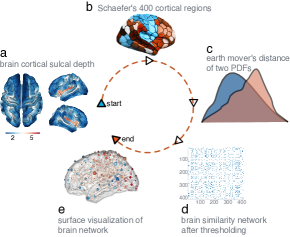
Figure 1: Flowchart of constructing the brain sulcal depth similarity network. a, First obtain the sulcal depth for each node in the brain surface space. b, Then, use the Schaefer 400 atlas to define the brain nodes. c, For each brain region, estimate their PDF of sulcal depth and calculate the earth mover’s distance between any paired brain regions, resulting in a $400\times 400$ similarity matrix with top 10% edges preserved (d), Convert the distance metric to similarity metric through sigmoid function. e, Surface plot of the brain sulcal depth similarity network.

Datasets for multi-class classification. To explore the ability of DHC-E in multi-class classification tasks, following the above strategies, datasets M1-M8 (See SI. Sec. B.2 for more details) were constructed.

3.2.2 Baseline Methods

We compared DHC-E with the three baselines:

• GL2vec Chen and Koga (2019): GL2vec: Graph Embedding Enriched by Line Graphs with Edge Features.

• IGE Galland and Lelarge (2019): Invariant Embedding for Graph Classification.

• Graph2vec Narayanan et al. (2017): Graph2vec: Learning Distributed Representations of Graphs.

3.2.3 Evaluation metrics

Accuracy (ACC) and F1 scores (F1) Riesen and Bunke (2010) are used to quantify the performance of graph classification results. The better the performance of graph classification is, the larger the values of ACC and F1 will be.

3.2.4 Graph classification

Given a graph set $\mathbb{G}=\{G_{1},G_{2},...,G_{n}\}$, where $G_{i}=(V_{i},E_{i},l_{i})$ with node set $V_{i}$, edge set $E_{i}$ and label $l_{i}$ denoting its category, implementing DHC-E on each $G_{i}$ in $\mathbb{G}$ produces $n$ whole graph embeddings as

$$\{(H_{i,1},...,H_{i,s_{i}})|i=1,2,..,n\},$$ (5)

where $H_{i,j}$ is the Shannon entropy of $G_{i}$ in the $j$-th iteration within the total $s_{i}$ convergence steps of the DHC updating process. Then, these embeddings are replenished with their last elements to align in dimension $s_{\operatorname{max}}$. Finally, an $n\times s_{\operatorname{max}}$ matrix is constructed as the input of KNN classifier. After comparing with other classifiers such as support vector machine (SVM), KNN performed more efficiently and still effectively. The pseudo code of DHC-E for graph classification is shown in Algorithm 1.

Algorithm 1. DHC-E for graph classification Input: A set of $n$ graphs $\mathbb{G}=\{G_{1},G_{2},...,G_{n}\},G_{i}=(V_{i},E_{i},l_{i})$. Output: the classification results $l_{1}^{\prime},l_{2}^{\prime},...,l_{n}^{\prime}$ of $\mathbb{G}$. 1  : DHC_EntropyMatrix = [ ]: 2  : for each $G_{i}=(V_{i},E_{i},l_{i})$ in $\mathbb{G}$: 3  :  Hi = [$d_{1},d_{2},...,d_{\operatorname{|V_{i}|}}$] 4  :  $H_{i,0}$ = ShannonEntopy(Hi) 5  :  j=1: 6  :  while true: 7  :   HiUpdated = DHC_UpdatingProcess (Hi) 8  :   if HiUpdated is equal to Hi: 9  :    break 10:   else: 11:    $H_{i,j}$ = ShannonEntropy(HiUpdated) 12:    Hi = HiUpdated 13:    $j=j+1$ 14:  add $[H_{i,0},H_{i,1},...]$ to DHC_EntropyMatrix by row 15: DHC_EntropyMatrix = DimensionAlignment(DHC_EntropyMatrix) 16: $l_{1}^{\prime},l_{2}^{\prime},...,l_{n}^{\prime}=$KNN(DHC_EntropyMatrix)

To ensure the fairness of performance comparison, the embeddings obtained from different models were taken as the input of a common KNN classifier with fixed hyperparameters for graph classification (see line 16 in Algorithm 1). For every model, its overall performance is averaged by 500 runs of the KNN classifier with 10-fold cross-validation.

4 Experimental results

The ACC and F1 results for DHC-E and baselines on binary and multi-class classification tasks are summarized in Figure. 2, Table. 2 and Table. 3, respectively, where the corresponding stability results are also shown. The time complexity results are presented in Table. 4.

Overall, DHC-E achieves the first rank across all the datasets based on the mean classification value and provides a better trade-off between the accuracy, stability, and time complexity. Additionally, an application of DHC-E on graph visualization is shown in Figure. 3.

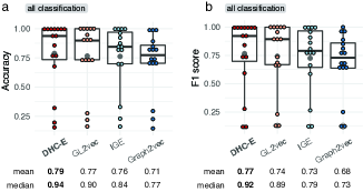
Figure 2: Classification performance of different graph embedding models. The plots were sorted by their mean values (in descending order). For all cases (B1-B8 and M1-M8), the accuracy and F1 score is presented in a and b, respectively. The black dots indicate the mean classification value of each model.

4.1 Results on binary graph classification

For binary graph classification, the ACC and F1 results for DHC-E and baselines are summarized in Table. 2, in which the eight datasets are classified into three different subtasks for binary graph classification (i.e., the subtasks based on categorized datasets by simulation, sub-categorized datasets from the real world, and categorized datasets), where the ACC and F1 results for evaluated models are averaged, respectively. The hyperparameter settings of baselines follow the default values in the python package, named karate club, as shown in SI. Sec. B.3. Each result is calculated by averaging over 500 runs on independently random split train-test sets. Clearly, DHC-E outperforms other models for all three subtasks of binary classification.

Specifically, in comparing the overall performance of DHC-E with the weakest baseline on the three subtasks, DHC-E outperforms Graph2vec on the first subtask (i.e., B1, B2, and B3) by 16.59% and 22.69% over ACC and F1, respectively. Regarding the second subtask (B4, B5, and B6), the ACC and F1 results of DHC-E are 6.64% and 7.62% higher than those of Graph2vec, respectively. Similarly, on the third task (i.e., B7 and B8) DHC-E outperforms GL2vec by 5.12% and 5.37% over ACC and F1, respectively. Clearly, the DHC-E has been demonstrated that even a simple model can achieve good classification performance, and in some cases even outperform complex models.

These results indicate that the difficulty of graph sets to be classified may be distinctive under specific scenarios. Thus, one should make a trade-off between accuracy and stability (see Tables. 2 and 3), and time consuming (see Table. 4), in order to select appropriate models for graph classification.

datasets DHC-E Graph2vec IGE GL2vec ACC F1 ACC F1 ACC F1 ACC F1 B1 1.000 (0.000) 1.000 (0.000) 1.000 (0.000) 1.000 (0.000) 0.850 (0.000) 0.807 (0.000) 0.740 (0.032) 0.674 (0.036) B2 1.000 (0.000) 1.000 (0.000) 0.740 (0.028) 0.634 (0.033) 1.000 (0.000) 1.000 (0.000) 1.000 (0.000) 1.000 (0.000) B3 1.000 (0.000) 1.000 (0.000) 0.833 (0.029) 0.811 (0.036) 0.962 (0.000) 0.958 (0.000) 1.000 (0.000) 1.000 (0.000) Avg. 1.000 (0.000) 1.000 (0.000) 0.858 (0.019) 0.815 (0.023) 0.937 (0.000) 0.922 (0.000) 0.913 (0.011) 0.891 (0.012) Imp. - - +16.59% +22.69% +6.67% +8.49% +9.48% +12.20% B4 0.857 (0.011) 0.841 (0.012) 0.704 (0.012) 0.692 (0.012) 0.875 (0.003) 0.862 (0.004) 0.745 (0.018) 0.736 (0.018) B5 0.755 (0.014) 0.733 (0.015) 0.704 (0.031) 0.668 (0.039) 0.701 (0.000) 0.663 (0.000) 0.717 (0.030) 0.686 (0.037) B6 0.677 (0.031) 0.593 (0.036) 0.738 (0.054) 0.653 (0.073) 0.694 (0.057) 0.587 (0.079) 0.740 (0.000) 0.654 (0.000) Avg. 0.763 (0.019) 0.722 (0.021) 0.715 (0.032) 0.671 (0.041) 0.757 (0.020) 0.704 (0.028) 0.734 (0.016) 0.692 (0.018) Imp. - - +6.64% +7.62% +0.80% +2.61% +3.93% +4.36% B7 1.000 (0.000) 1.000 (0.000) 0.977 (0.005) 0.976 (0.005) 1.000 (0.000) 1.000 (0.000) 0.903 (0.011) 0.898 (0.012) B8 1.000 (0.000) 1.000 (0.000) 0.975 (0.006) 0.949 (0.014) 1.000 (0.000) 1.000 (0.000) 1.000 (0.000) 1.000 (0.000) Avg. 1.000 (0.000) 1.000 (0.000) 0.976 (0.006) 0.962 (0.010) 1.000 (0.000) 1.000 (0.000) 0.951 (0.006) 0.949 (0.006) Imp. - - +2.46% +3.92% 0.00% 0.00% +5.12% +5.37%

Table 2: Results on binary graph classification tasks.

4.2 Results on multi-class graph classification

For multi-class graph classification tasks, the ACC and F1 results for DHC-E and baselines are summarized in Table. 3, in which the eight datasets are classified into three different subtasks for multi-class graph classification (i.e., the subtasks based on categorized datasets by simulation, sub-categorized datasets from the real world, and categorized datasets), where the ACC and F1 results for evaluated methods are averaged, respectively. The hyperparameter settings of baselines follow the default values in the python package, named karate club, as shown in SI. Sec. B.3. Each result is calculated by averaging over 500 runs with 10-fold cross validation. It shows that the overall advantages of DHC-E are still satisfactory on the three subtasks compared with that of baseline, but not as prominent as that on binary graph classification tasks.

Specifically, on the first subtask (i.e., M1, M2, and M3), although DHC-E is 1.32 % and 1.84% lower than GL2vec over ACC and F1, respectively, it still significantly outperforms IGE and Graph2vec, where the ACC and F1 results of DHC-E are 12.29% and 15.94% higher than those of IGE, and 23.34% and 30.28% higher than those of Graph2vec, respectively. As for the second subtask (i.e., M4, M5, and M6), DHC-E achieves the accuracy in the middle level among all models. On the third subtask (i.e., M7 and M8), DHC-E is slightly inferior in the evaluated models. Its ACC and F1 results are 3.83% and 6.19 % lower than that of the best-performed baseline (i.e., GL2vec), respectively.

Besides, the overall accuracy of all models on the second subtask (i.e., M4, M5, and M6) is much worse compared with that on the other two subtasks, as shown in Table. 3. This result reveals that the effective method for multi-class classification remains to be a great challenge today.

datasets DHC-E Graph2vec IGE GL2vec ACC F1 ACC F1 ACC F1 ACC F1 M1 1.000 (0.000) 1.000 (0.000) 0.820 (0.000) 0.775 (0.000) 0.827 (0.000) 0.771 (0.000) 1.000 (0.000) 1.000 (0.000) M2 0.950 (0.012) 0.932 (0.018) 0.704 (0.059) 0.640 (0.067) 0.923 (0.000) 0.909 (0.000) 1.000 (0.000) 1.000 (0.000) M3 0.925 (0.010) 0.913 (0.012) 0.807 (0.026) 0.768 (0.031) 0.810 (0.000) 0.774 (0.000) 0.913 (0.001) 0.898 (0.001) Avg. 0.958 (0.007) 0.948 (0.010) 0.777 (0.028) 0.728 (0.033) 0.853 (0.000) 0.818 (0.000) 0.971 (0.000) 0.966 (0.000) Imp. - - +23.34% +30.28% +12.29% +15.94% -1.32% -1.84% M4 0.321 (0.013) 0.278 (0.013) 0.295 (0.030) 0.251 (0.028) 0.330 (0.000) 0.265 (0.000) 0.276 (0.029) 0.231 (0.026) M5 0.155 (0.007) 0.119 (0.006) 0.146 (0.015) 0.114 (0.013) 0.162 (0.000) 0.120 (0.000) 0.163 (0.014) 0.124 (0.012) M6 0.196 (0.011) 0.119 (0.008) 0.226 (0.025) 0.136 (0.019) 0.230 (0.000) 0.128 (0.000) 0.219 (0.024) 0.136 (0.019) Avg. 0.224 (0.010) 0.172 (0.009) 0.222 (0.024) 0.167 (0.020) 0.241 (0.000) 0.171 (0.000) 0.219 (0.022) 0.164 (0.019) Imp. - - +0.71% +2.84% -7.16% +0.56% +2.03% +4.83% M7 0.991 (0.002) 0.991 (0.002) 0.892 (0.010) 0.888 (0.011) 0.994 (0.000) 0.994 (0.000) 0.894 (0.011) 0.889 (0.012) M8 0.780 (0.005) 0.740 (0.003) 0.847 (0.009) 0.851 (0.010) 0.839 (0.000) 0.773 (0.000) 0.947 (0.006) 0.956 (0.005) Avg. 0.885 (0.003) 0.866 (0.002) 0.870 (0.010) 0.870 (0.011) 0.916 (0.000) 0.883 (0.000) 0.921 (0.009) 0.923 (0.009) Imp. - - +1.84% -0.47% -3.38% -2.01% -3.83% -6.19%

Table 3: Results on multi-class graph classification tasks.

4.3 Stability analysis

Stability, as opposed to the deviation from the averaged performance of a model, is also an important metric for assessment, for it quantifies the potential of a model to reach its best performance compared to baselines, which determines the cost of experiments.

The corresponding standard deviations of the ACC and F1 results for DHC-E and baselines on datasets for both binary classification and multi-class classification are summarized in Tables. 2 and 3, which reveals the stability of different methods over 500 runs with split train-test sets. For a model, the lower the averaged standard deviations of ACC and F1 results, the higher the model’s stability. Tables. 2 and 3 show the overall averaged standard deviations of ACC results on IGE, DHC-E, GL2vec, and Graph2vec are 0.004, 0.007, 0.011, 0.021, respectively, and the standard deviations of F1-score results on the four models are 0.005, 0.008, 0.011, 0.025, respectively, indicating that DHC-E has satisfactory stability among the evaluated models.

4.4 Time complexity analysis

Here, we systemically investigate the time complexity of DHC-E and three baseline models to make a more comprehensive understanding of the trade-off between accuracy and time complexity.

The corresponding consuming time of DHC-E and baselines on different datasets is summarized in Table. 4, in which the time consumption, measured in seconds, is averaged from 500 separate runs. DHC-E achieves the second-best efficiency in overall time complexity among all of the four models, as shown in Table. 4, resulting in 69.23% higher time consumption than Graph2vec. However, DHC-E has 150.13% and 1520.47% lower time consumption than IGE and GL2vec, respectively.

The researcher can choose different models depending on the specific situation. It should be emphasized that our Python code of DHC-E is not explicitly optimized, and there is still some room for performance improvement. In addition, we also provide Julia and MATLAB code of DHC-E, both of which are fast and can complete the B6 task in 1.8s and 4s, separately, on a personal computer [MacBook Pro (Retina, 13-inch, Early 2015); Processor 2.7 GHz Dual-Core Intel Core i5].

datasets Time (DHC-E) Time (Graph2vec) Time (IGE) Time (GL2vec) B1 3.230 2.280 3.378 3.461 B2 5.812 2.668 7.317 69.491 B3 9.101 3.866 42.268 636.969 B4 5.365 6.518 13.048 10.688 B5 7.143 10.569 16.902 13.385 B6 20.399 3.351 50.065 495.777 B7 8.253 6.792 14.966 17.311 B8 22.100 7.940 67.482 473.768 M1 5.640 2.466 4.840 4.506 M2 6.868 3.359 10.619 191.478 M3 11.254 6.543 70.885 807.907 M4 6.608 11.068 18.957 9.934 M5 25.229 7.398 31.545 23.254 M6 6.401 10.825 17.899 10.081 M7 9.215 8.386 25.682 10.549 M8 46.286 23.503 101.683 444.753 Avg. 12.432 7.346 31.096 201.457

Table 4: Time complexity analysis.

4.5 Graphs visualization with DHC-E features

We conducted an exploratory analysis in graph visualization applications to verify whether the DHC-E embedding method can adequately express different graphs in a two-dimensional space. First, we generated 20 small-world networks, 20 BA networks, and 20 random networks. Then, we combined these 60 networks with 20 ASD brain networks into a new dataset. To that end, we performed the DHC-E analysis on these 80 graphs and obtained the whole graph embedding for each graph. Subsequently, we performed principal component analysis (PCA) on the obtained embedded features to further reduce the embedding features to two dimensions. We observed that the first two PCs explain about 99.6% of the total variability for the whole graph embedding. We found that it can cluster together graphs in the same category, which show the potential applications of DHC-E in lower-dimensional morphospace representation of graphs, as illustrated by Figure. 3 in details.

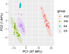
Figure 3: Lower-dimension morphospace representation of graph with DHC-E features, we use the PCA to reduce the DHC-E whole graph embedding features into a two-dimension space and find that the DHC-E features can cluster together graphs in the same category. ASD, autism spectrum disorders’ brain network; SW, small-world network; BA, scale-free network; ER, random network.

5 Conclusion and further consideration

In this study, we only consider the whole graph embedding rather than node or edge embeddings. We propose a simple, hyperparameter-free, and explainable graph embedding method and evaluate its performance on classification tasks using different datasets. We found that DHC-E is comparable but more straightforward than most sophisticated methods of graph embedding. By using DHC-E, we avoid problems such as tedious hyperparameters tuning and poor interpretability. As it stands, the DHC-E method shows good classification performance, stability and promising potential in lower-dimensional graph visualization. Additionally, DHC-E can be integrated with the current model to verify whether it can improve the classification performance and we built a brain network benchmark for further researches. Among researchers in interdisciplinary fields, a model that works out-of-the-box, has fewer parameters, and has moderately high performance may prove useful, and DHC-E may provide some guidance for future research into simple and effective whole graph embedding models.

6 Data and code available

Supporting Information, data and codes are available at https://github.com/HW-HaoWang/DHC-E

7 Acknowledgements

This work is supported by the National Natural Science Foundation of China (Nos. 61673150, 11622538), the Science Strength Promotion Program of the University of Electronic Science and Technology of China (No. Y030190261010020), and the China Scholarship Council (No. 201906070121).

References

- Barabási [2009] A. Barabási. Scale-free networks: A decade and beyond. Science, 325:412 – 413, 2009.
- Belkin and Niyogi [2003] Mikhail Belkin and P. Niyogi. Laplacian eigenmaps for dimensionality reduction and data representation. Neural Computation, 15:1373–1396, 2003.
- Bordes et al. [2013] Antoine Bordes, Nicolas Usunier, Alberto Garcia-Duran, Jason Weston, and Oksana Yakhnenko. Translating embeddings for modeling multi-relational data. In Advances in Neural Information Processing Systems, pages 2787–2795, 2013.
- Cao et al. [2015] Shaosheng Cao, Wei Lu, and Qiongkai Xu. Grarep: Learning graph representations with global structural information. In Proceedings of the 24th ACM International Conference on Information and Knowledge Management, pages 891–900, 2015.
- Chen and Koga [2019] Hong Chen and Hisashi Koga. Gl2vec: Graph embedding enriched by line graphs with edge features. In International Conference on Neural Information Processing, pages 3–14. Springer, 2019.
- Dorogovtsev et al. [2006] Sergey N Dorogovtsev, Alexander V Goltsev, and Jose Ferreira F Mendes. K-core organization of complex networks. Physical Review Letters, 96(4):040601, 2006.
- Galland and Lelarge [2019] Alexis Galland and Marc Lelarge. Invariant embedding for graph classification. In ICML 2019 Workshop on Learning and Reasoning with Graph-Structured Data, 2019.
- Grover and Leskovec [2016] Aditya Grover and Jure Leskovec. node2vec: Scalable feature learning for networks. In Proceedings of the 22nd ACM SIGKDD International Conference on Knowledge Discovery and Data Mining, pages 855–864, 2016.
- Hirsch [2005] Jorge E Hirsch. An index to quantify an individual’s scientific research output. Proceedings of the National academy of Sciences, 102(46):16569–16572, 2005.
- Janssens et al. [2022] Jasper Janssens, Sara Aibar, Ibrahim Ihsan Taskiran, Joy N. Ismail, Alicia Estacio Gomez, Gabriel N. Aughey, Katina I. Spanier, Florian V. De Rop, Carmen Bravo González-Blas, Marc S. Dionne, Krista Grimes, Xiao-Jiang Quan, Dafni Papasokrati, Gert Hulselmans, Samira Makhzami, Maxime de Waegeneer, Valerie Christiaens, Tony D. Southall, and Stein Aerts. Decoding gene regulation in the fly brain. Nature, 2022.
- Lü et al. [2016] Linyuan Lü, Tao Zhou, Qian-Ming Zhang, and H Eugene Stanley. The h-index of a network node and its relation to degree and coreness. Nature Communications, 7(1):1–7, 2016.
- Mikolov et al. [2013] Tomas Mikolov, Ilya Sutskever, Kai Chen, Greg S Corrado, and Jeff Dean. Distributed representations of words and phrases and their compositionality. In Advances in Neural Information Processing Systems, pages 3111–3119, 2013.
- Morris et al. [2020] Christopher Morris, Nils M. Kriege, Franka Bause, Kristian Kersting, Petra Mutzel, and Marion Neumann. Tudataset: A collection of benchmark datasets for learning with graphs. In ICML 2020 Workshop on Graph Representation Learning and Beyond (GRL+ 2020), 2020.
- Narayanan et al. [2017] Annamalai Narayanan, Mahinthan Chandramohan, Rajasekar Venkatesan, Lihui Chen, Yang Liu, and Shantanu Jaiswal. graph2vec: Learning distributed representations of graphs. arXiv preprint arXiv:1707.05005, 2017.
- Perozzi et al. [2014] Bryan Perozzi, Rami Al-Rfou, and Steven Skiena. Deepwalk: Online learning of social representations. In Proceedings of the 20th ACM SIGKDD International Conference on Knowledge Discovery and Data Mining, pages 701–710, 2014.
- Riesen and Bunke [2010] Kaspar Riesen and Horst Bunke. Graph classification and clustering based on vector space embedding, volume 77. World Scientific, 2010.
- Shannon [1948] Claude E Shannon. A mathematical theory of communication. The Bell System Technical Journal, 27(3):379–423, 1948.
- Shervashidze et al. [2011] Nino Shervashidze, Pascal Schweitzer, Erik Jan Van Leeuwen, Kurt Mehlhorn, and Karsten M Borgwardt. Weisfeiler-lehman graph kernels. Journal of Machine Learning Research, 12(9), 2011.
- Tenenbaum [2002] J. Tenenbaum. The isomap algorithm and topological stability. Science, 295:9 – 9, 2002.
- Vasconcelos et al. [2021] Vítor V Vasconcelos, Sara M Constantino, Astrid Dannenberg, Marcel Lumkowsky, Elke Weber, and Simon Levin. Segregation and clustering of preferences erode socially beneficial coordination. Proceedings of the National Academy of Sciences, 118(50), 2021.
- Verma and Zhang [2017] Saurabh Verma and Zhi-Li Zhang. Hunt for the unique, stable, sparse and fast feature learning on graphs. In Proceedings of the 31st International Conference on Neural Information Processing Systems, pages 87–97, 2017.
- Wu et al. [2018] Huijun Wu, Hao Wang, and Linyuan Lü. Individual t1-weighted/t2-weighted ratio brain networks: Small-worldness, hubs and modular organization. International Journal of Modern Physics C, 29(05):1840007, 2018.
- Yanardag and Vishwanathan [2015] Pinar Yanardag and SVN Vishwanathan. Deep graph kernels. In Proceedings of the 21th ACM SIGKDD International Conference on Knowledge Discovery and Data Mining, pages 1365–1374, 2015.
- Zhang et al. [2018] Daokun Zhang, Jie Yin, Xingquan Zhu, and Chengqi Zhang. Network representation learning: A survey. IEEE transactions on Big Data, 6(1):3–28, 2018.