Photometric variability of the pre-main sequence stars towards the Sh 2-190 region

Abstract

We present the results from our time-series imaging data taken with the 1.3m Devasthal fast optical telescope and 0.81m Tenagara telescope in $V$, $R_{c}$, $I_{c}$ bands covering an area of $\sim 18^{\prime}.4\times 18^{\prime}.4$ towards the star-forming region Sh 2-190. This photometric data helped us to explore the nature of the variability of pre-main sequence (PMS) stars. We have identified 85 PMS variables, i.e., 37 Class ii and 48 Class iii sources. Forty-five of the PMS variables are showing periodicity in their light curves. We show that the stars with thicker discs and envelopes rotate slower and exhibit larger photometric variations compared to their disc-less counterparts. This result suggests that rotation of the PMS stars is regulated by the presence of circumstellar discs. We also found that the period of the stars show a decreasing trend with increasing mass in the range of $\sim$0.5-2.5 M_⊙. Our result indicates that most of the variability in Class ii sources is ascribed to the presence of thick disc, while the presence of cool spots on the stellar surface causes the brightness variation in Class iii sources. X-ray activities in the PMS stars were found to be at the saturation level reported for the main sequence (MS) stars. The younger counterparts of the PMS variables are showing less X-ray activity hinting towards a less significant role of a stellar disc in X-ray generation.

1 Introduction

Circumstellar discs are an integral part of pre-main sequence (PMS) stars and are potential sites for planet formation (Hillenbrand, 2002). Depending on their evolutionary stages PMS stars are classified as Class i, Class ii and Class iii objects. Class i objects are deeply embedded protostars with in-falling material from the envelope and circumstellar discs through which material is accreted onto the growing star. Class ii objects possess thick circumstellar disc and residual envelope and are found to accrete material from the disc through magnetic channels connecting the disc and the stars, while the Class iii objects are yet to reach the main-sequence (MS) with depleted or no accretion discs (Greene et al., 1994; Carney et al., 2016). Based on their mass, PMS stars are also classified as T Tauri stars (TTSs) ($\lesssim$ 3 M_⊙) and Herbig Ae/Be stars (3-10 M_⊙). On the basis of the strength of H$\alpha$ emission, TTSs are further classified into classical TTSs (CTTSs; equivalent width (EW)$>$10Å) and weak-line TTSs (WTTSs; EW$\leq$10Å) (Herbig & Bell, 1988; Strom et al., 1989). CTTSs and WTTSs more or less resemble Class ii and Class iii objects, respectively. Brightness variability is one of the distinguishing features of stars in their TTS phase (Joy, 1945). These variations are attributed to a combination of physical processes operating at and near their surfaces (Cody et al., 2014). WTTSs tend to display periodic light curves (LCs) due to the presence of an asymmetric distribution of cool or dark spots which modulate the observed luminosity of the stars during its rotation (Grankin et al., 2008; Rodríguez-Ledesma et al., 2009). On the other hand CTTSs display more complex signatures of different time-scales categorized as stochastic events (e.g., Rucinski et al., 2008; Siwak et al., 2011), occasional fading/brightening (Cody & Hillenbrand, 2010; Guo et al., 2018) and periodic/semi-periodic (Herbst et al., 1994) variability. The first category is caused by time variable accretion from the circumstellar disc onto the surface of the star where the accretion zones or hot spots are non-uniformly distributed (Herbst et al., 2007; Cody et al., 2014). In addition, CTTSs occasionally exhibit short (1-5 days, called dippers) and/or long (weeks to years, called faders) term extinction events caused when the star is occulted by disc components at or near the disc truncation radius (Cody et al., 2014; Alencar et al., 2010; Bouvier et al., 2013; Loomis et al., 2017; Guo et al., 2018). Like WTTSs, CTTSs can also show periodic/semi-periodic brightness variation due to either presence of hot and/or cool spots on their surface or any disc wrap which periodically occults the central star (Bouvier et al., 2007; McGinnis et al., 2015). Most of the variability in Herbig Ae/Be stars, the intermediate-mass counterpart of CTTSs, are caused due to obscuration by circumstellar dust (Herbst et al., 2007; Semkov, 2011). Studying variability properties of PMS stars can lead to a better understanding of the physical processes happening in their evolution and imposing constraints on the stellar evolutionary models. Recent work on PMS variability can be found, e.g., in Fritzewski et al. (2016); Teixeira et al. (2018); Xue et al. (2019), but still we are not able to construct a complete paradigm for the stars and disc evolution.

In this study, we have identified PMS variables, both periodic and non-periodic, in the Sh 2-190 star-forming region and investigate the correlations between their physical properties (period, amplitude, age, mass, IR-excess, accretion rate, X-ray activities, etc.). Then we discuss the physical processes responsible for the early evolution of the central star and the disc. We organize this paper into six sections. Following the introduction section, we present an overview of the Sh 2-190 star-forming region in Section 2. We describe the observation and data reduction in Section 3. The identification of PMS variables and derivation of their physical parameters are presented in Section 4. Physical processes responsible for the PMS variability are discussed in Section 5. We conclude our results in Section 6.

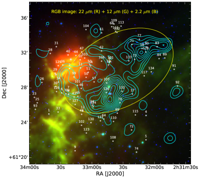
Figure 1: Color-composite image obtained by using the 2.2 $\mu$m $K_{s}$ (blue, 2MASS), 12 $\mu$m (green, $WISE$) and 22 $\mu$m (red, $WISE$) images of the $\sim 18^{\prime}.4\times 18^{\prime}.4$ FOV around the Sh 2-190 H ii region. The cyan contours represent the $K_{s}$ band stellar surface density distribution. The yellow ellipse represents the extent of the cluster IC 1805. Identified PMS variable stars are encircled along with their identification numbers (see text for details).

2 Overview of Sh 2-190

Sh 2-190 is a young (age $\sim$ 2.3 Myr, Panwar et al., 2017) star forming region located at a moderate distance (2.0 kpc, Straižys et al., 2013) consisting the central cluster IC 1805 ($\alpha_{2000}$ = 02^h32^m42^s, $\delta_{2000}$ = +61^∘27^m00^s) surrounded by the giant molecular cloud W4 in the Perseus spiral arm of the galaxy. There are nine O-type stars in IC 1805 cluster, which are considered to be the triggering source of star-formation activities in this region (Sung et al., 2017). The infrared color-composite image of the studied region of the Sh 2-190 is shown in Figure 1. Heated dust grains (22 $\micron$ emission, red) can be seen adjacent to the stellar overdensity region. This warm dust is also surrounded by 12 $\mu$m emission (green). $WISE$ 12 $\mu$m band covers the prominent PAH features at 11.3 $\mu$m, indicative of photon dominant region (PDR) under the influence of feedback from massive stars (see e.g., Peeters et al., 2004). This fact denotes that we are dealing with a site showing signatures of recent star-formation activities. Naturally, this region is also known to host many young stellar objects (YSOs) (e.g., Sung et al., 2017; Panwar et al., 2017). All of these features make this cluster an ideal site to look for PMS variable stars and to study their properties.

Table 1: Observation log for Sh 2-190 region.

Date of observation	Telescope	N$\times$Exp.(s)	Number of nights	Filter
30.09.2012-20.03.2013	0.81m Tenagara	230$\times$120, 240$\times$60, 246$\times$100	82, 81, 82	$I_{c}$,$R_{c}$,$V$
	Telescope
28.06.2018-16.03.2019	ZTF	107$\times$30, 107$\times$30	107, 107	$zg$,$zr$
06.12.2018	DFOT	05$\times$120, 05$\times$300	01	$I_{c}$ ,$V$
09.01.2019	DFOT	04$\times$120, 04$\times$300	01	$I_{c}$ ,$V$
01.02.2019	DFOT	01$\times$120, 01$\times$180	01	$I_{c}$,$R_{c}$
02.02.2019	DFOT	11$\times$120, 11$\times$180, 11$\times$300	01	$I_{c}$,$R_{c}$,$V$
03.02.2019	DFOT	09$\times$120, 09$\times$180, 09$\times$300	01	$I_{c}$,$R_{c}$,$V$
05.02.2019	DFOT	02$\times$120, 02$\times$180, 02$\times$300	01	$I_{c}$,$R_{c}$,$V$
09.03.2019	DFOT	03$\times$120, 03$\times$180, 01$\times$300	01	$I_{c}$,$R_{c}$,$V$
10.03.2019	DFOT	03$\times$120, 03$\times$180, 01$\times$300	01	$I_{c}$,$R_{c}$,$V$
26.10.2019	DFOT	05$\times$180, 05$\times$300	01	$R_{c}$,$V$
27.10.2019	DFOT	03$\times$180, 03$\times$300	01	$R_{c}$,$V$
28.10.2019	DFOT	08$\times$180, 08$\times$300	01	$R_{c}$,$V$
01.11.2019	DFOT	25$\times$120, 25$\times$180, 25$\times$300	01	$I_{c}$,$R_{c}$,$V$
01.12.2019	DFOT	27$\times$120, 27$\times$180, 27$\times$300	01	$I_{c}$,$R_{c}$,$V$
25.12.2019	DFOT	03$\times$120, 04$\times$180, 03$\times$300	01	$I_{c}$,$R_{c}$,$V$
18.02.2020	DFOT	04$\times$120, 04$\times$180, 04$\times$300	01	$I_{c}$,$R_{c}$,$V$

3 Observation and data reduction

3.1 Optical photometric data

Optical photometric observations of Sh 2-190 were taken in $V$, $R_{c}$, $I_{c}$ bands during September 2012 to March 2013 with 0.81 m Tenagara Automated Telescope (South Arizona) and from December 2018 to February 2020 using the 1.3 m Devasthal Fast Optical Telescope (DFOT, India). DFOT has a 2048 $\times$ 2048 pixel square CCD which covers $18^{\prime}.4\times 18^{\prime}.4$ field of view (FOV), whereas Tenagara telescope covers $14^{\prime}.6\times 14^{\prime}.6$ FOV with a 1024 $\times$ 1024 pixel square CCD. The FITS files of $18^{\prime}.4\times 18^{\prime}.4$ FOV in $zg$ and $zr$ bands were also downloaded from Zwicky Transient Facility (ZTF) archive (Masci et al., 2019) giving time-series images from June 2018 to March 2019. In total, the object was observed on 96, 94, 94, 107 and 107 nights in $V$, $R_{c}$, $I_{c}$, $zg$ and $zr$ bands, respectively, and we use 354, 344, 327, 107 and 107 frames of the five bands in the following analysis. Details of observation are given in Table 1. We have used standard data reduction procedures for the image cleaning, photometry and astrometry (for details, see Sinha et al., 2020). The photometric detection from different telescopes were cross-matched using their astrometry within a search radius of 1 arcsec. The instrumental magnitudes in $V$, $R_{c}$, $I_{c}$ bands were converted to standard $V$, $R_{c}$ and $I_{c}$ magnitudes, also $zg$ and $zr$ magnitudes were converted to standard $R_{c}$, $I_{c}$ magnitudes using the already published photometry of stars in the same region (Sung et al., 2017).

3.2 Archival Photometric data

For our analyses, we have also used the following archival data covering various wavelengths :

(i) NIR $JHKs$ photometric data were taken from the 2MASS All-Sky Point Source Catalog (Skrutskie et al., 2006; Cutri et al., 2003).

(ii) Spitzer-IRAC observations at 3.6, 4.5, 5.8 and 8.0 $\mu$m were taken from the GLIMPSE360 Catalog and Archive (Werner et al., 2004).

(iii) MIR data at 3.4, 4.6, 12 and 22 $\mu$m were taken from the Wide-field Infrared Survey Explorer (WISE) All-sky Survey Data release (Wright et al., 2010).

(iv) X-ray data were taken from ‘The massive Star-Forming Regions Omnibus X-ray Catalog’ (Townsley et al., 2014).

4 Results and Analysis

4.1 Structure of the cluster

To study the stellar surface density distribution of the Sh 2-190 region, we generated surface density contours for a sample of stars taken from the 2MASS All-Sky Point Source Catalog, covering $18^{\prime}.4\times 18^{\prime}.4$ FOV around this region (for details, see Sinha et al., 2020). These density contours are plotted in Figure 1 as cyan curves. The lowest contour is 1$\sigma$ above the mean stellar density (i.e., 9.4$\pm$2.8 stars/arcmin²) and the step size is equal to 1$\sigma$ (2.8 stars/arcmin²). Stellar density enhancements at ($\alpha_{2000}$, $\delta_{2000}$) $\sim$ ($02^{h}32^{m}37^{s}.2$, $+61^{\circ}30^{\prime}23^{\prime\prime}.7$) and $\sim$ ($02^{h}32^{m}22^{s}.5$, $+61^{\circ}31^{\prime}56^{\prime\prime}$) can easily be seen from the contours. With these two peaks the shape of the cluster looks like an ellipse (shown with a yellow ellipse in Figure 1) with a major and minor axis of 7 arcmin and 4.5 arcmin, respectively. On the basis of the radial density profile, Panwar et al. (2017) have estimated the cluster radius as 7 arcmin which is comparable with the present estimate.

Table 2: Sample of stars identified as members in the Sh 2-190. The complete table is available in the electronic form only.

ID	$\alpha_{(2000)}$	$\delta_{(2000)}$	$V$	$R_{c}$	$I_{c}$	$\mu_{\alpha}$	$\mu_{\delta}$	Parallax	Probability	$G$	$G_{BP}-G_{RP}$
	$(degrees)$	$(degrees)$	(mag)	(mag)	(mag)	(mas/yr)	(mas/yr)	(mas)	(%)	(mag)	(mag)
M1	38.300182	61.354942	15.046 $\pm$ 0.004	14.516 $\pm$ 0.008	13.968 $\pm$ 0.007	-0.66 $\pm$ 0.03	-0.85$\pm$ 0.05	0.39$\pm$ 0.03	97	14.744	1.182
M2	38.396862	61.390205	18.705 $\pm$ 0.001	17.689 $\pm$ 0.011	16.615 $\pm$ 0.001	-0.60 $\pm$ 0.15	-0.50$\pm$ 0.19	0.48$\pm$ 0.12	95	17.779	2.120
M3	38.112164	61.312714	19.969 $\pm$ 0.004	19.005 $\pm$ 0.005	18.074 $\pm$ 0.001	-1.12 $\pm$ 0.36	-0.49$\pm$ 0.46	0.34$\pm$ 0.30	84	19.218	1.683
M4	38.189682	61.441990	18.045 $\pm$ 0.037	16.868 $\pm$ 0.005	15.791 $\pm$ 0.010	-0.72 $\pm$ 0.09	-0.93$\pm$ 0.13	0.41$\pm$ 0.07	96	16.928	2.262

$V$, $R_{c}$ and $I_{c}$ data taken from Sung et al. (2017).

4.2 Membership

We have estimated the membership probability of stars for their association with Sh 2-190 using the method described in Balaguer-Núnez et al. (1998). This method has been extensively used recently (cf. Sinha et al., 2020; Sharma et al., 2020; Kaur et al., 2020; Pandey et al., 2020). For this, we have used $Gaia$ DR2 proper motion (PM) data of stars located within $18^{\prime}.4\times 18^{\prime}.4$ FOV in the Sh 2-190 region. We first construct the frequency distributions of cluster stars ($\phi^{\nu}_{c}$) and field stars ($\phi^{\nu}_{f}$) using the equations 3 and 4 of Balaguer-Núnez et al. (1998). The input parameters such as the center of Proper motion ($\mu_{\alpha}$cos($\delta$) = -0.75 mas yr^-1, $\mu_{\delta}$ = -0.70 mas yr^-1), its dispersion for the cluster stars ($\sigma_{c}$, $\sim$0.06 mas yr^-1) and field proper motion center ($\mu_{xf}$ = -0.003 mas yr^-1, $\mu_{yf}$ = -0.536 mas yr^-1), field intrinsic proper motion dispersion ($\sigma_{xf}$ = 3.35 mas yr^-1, $\sigma_{yf}$ = 3.21 mas yr^-1) are estimated similarly as have been discussed in our earlier work (Sinha et al., 2020). The membership probability (ratio of the distribution of cluster stars with all the stars) for the $i^{th}$ star is then estimated using the equation (1).

$$P_{\mu}(i)={{n_{c}\times\phi^{\nu}_{c}(i)}\over{n_{c}\times\phi^{\nu}_{c}(i)+n_{f}\times\phi^{\nu}_{f}(i)}}$$ (1)

where $n_{c}$ (=0.12) and $n_{f}$ (=0.88) are the normalized numbers of stars for the cluster and field regions ($n_{c}$+$n_{f}$ = 1), respectively.

The membership probability derived as above and parallax are plotted as a function of $G$ magnitude in the top and bottom panels of Figure 2. As can be seen a high membership probability (P${}_{\mu}\geqslant$ 80%) extends down to $G$ $\sim$ 20 mag. The bottom panel of Figure 2 displays the parallax of the same stars as a function of $G$ magnitude. Except few outliers, most of the stars with high membership probability (P${}_{\mu}\geqslant$ 80%) follow a tight distribution. We estimated the membership probability for 4551 stars and found 308 stars as cluster members (P${}_{\mu}\geqslant$ 80%). The details of these members are given in Table 2.

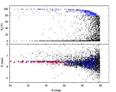
Figure 2: Membership probability (P_μ) and parallax ($\Pi$) as a function of $G$ magnitude for all the stars (black dots). The probable member stars (P${}_{\mu}\geq$ 80%) are shown by blue circles in both sub-panels. Red triangles indicate probable member stars with parallax errors better than 0.05 mas.

4.3 Distance and Reddening

We adopted the distances of the 64 identified member stars having parallax values with high accuracy (i.e. $error<0.05$ mas, shown as red triangles in the bottom panel of Figure 2) from Bailer-Jones et al. (2018). The average distance of these stars is $2.1\pm 0.2$ kpc, comparable to that obtained by Straižys et al. (2013) for IC 1805 (i.e., 2.0 kpc). We adopted the extinction value A${}_{V}=$ 2.46 mag for this cluster (Straižys et al., 2013).

Table 3: Sample of the identified PMS variables and their physical parameters as derived from CMD and/or SED. The complete table is available in the electronic form only.

ID	$\alpha_{(2000)}$	$\delta_{(2000)}$	$V$	$R_{c}$	$I_{c}$	Period	Amplitude	$\Delta(I_{c}-K_{s})$	$[3.6]-[4.5]$	Age$\dagger$
	(degrees)	(degrees)	(mag)	(mag)	(mag)	(days)	(mag)	(mag)	(mag)	(Myr)
V1	38.422897	61.417152	16.038$\pm$0.007	15.218$\pm$0.009	14.511$\pm$0.007	1.922$\pm$0.005	0.1$\pm$0.1	0.52$\pm$0.03	0.04$\pm$0.01	8.3$\pm$0.7
V2	38.340141	61.504135	16.342$\pm$0.012	15.312$\pm$0.006	14.419$\pm$0.010	1.123$\pm$0.002	0.1$\pm$0.1	0.05$\pm$0.02	0.05$\pm$0.01	1.0$\pm$0.2
V3	38.179836	61.516354	15.808$\pm$0.003	14.836$\pm$0.010	13.974$\pm$0.009	—	1.0$\pm$0.1	0.71$\pm$0.02	0.47$\pm$0.01	1.2$\pm$0.2
V4	38.033024	61.414288	16.102$\pm$0.002	15.211$\pm$0.008	14.358$\pm$0.010	—	1.3$\pm$0.1	1.38$\pm$0.02	0.41$\pm$0.01	2.8$\pm$0.6
ID	Mass$\dagger$	Data points*	$\chi^{2}*$	Age*	Mass*	Disc mass*	Disc accretion rate*	Log ($L_{X}/L_{bol}$)	Classification
	(M⊙)			(Myr)	(M⊙)	(M⊙)	(M⊙ $yr^{-1}$)
V1	1.8$\pm$0.0	10	6.8	5.5 $\pm$ 2.1	2.7 $\pm$ 0.6	4.7E-04 $\pm$ 3.7E-03	1.7E-10 $\pm$ 8.0E-10	-3.59	WTT
V2	2.5$\pm$0.1	10	3.6	2.1 $\pm$ 1.4	2.8 $\pm$ 0.4	2.0E-03 $\pm$ 7.7E-03	3.0E-09 $\pm$ 3.8E-08	-3.74	WTT
V3	3.0$\pm$0.1	14	12.4	1.8 $\pm$ 1.3	4.0 $\pm$ 1.3	1.9E-02 $\pm$ 3.3E-02	6.2E-08 $\pm$ 2.2E-07	-4.19	CTT
V4	2.4$\pm$0.1	14	14.1	3.8 $\pm$ 2.2	3.6 $\pm$ 0.8	1.1E-03 $\pm$ 6.7E-03	1.0E-08 $\pm$ 6.2E-08	-3.84	CTT

$\dagger$ : Parameters derived from CMD ; * Parameters derived from SED

4.4 Identification of variables

We performed differential photometry to identify variables in the $18^{\prime}.4\times 18^{\prime}.4$ FOV of the Sh 2-190 region (for details see Sinha et al., 2020). All the stars detected in our imaging survey (3461) are used in this analysis. Phase-folded LCs based on the period estimation from the Period software using the Lomb-Scargle (LS) periodogram (Lomb, 1976; Scargle, 1982) were used to identify the periodic variables (see for details, Sinha et al., 2020). The uncertainty in period estimation ($\delta$P) can be determined from the full width at half maximum (FWHM) of the main peak of the window function ($\nu_{FWHM}$), i.e, $\delta$P $=$ $\nu_{FWHM}\times$P² (see for details, Lamm et al., 2004). For the period range of 0.5d - 5d, the estimated errors are found to be in between $\sim$ 0.001d - 0.02d. To verify whether the peak corresponding to the estimated period in the LS power spectrum has significant signal, it has been related to a false alarm probability (FAP). FAP is a probability of finding a peak similar to the estimated period in a random data set (Rodríguez-Ledesma et al., 2009). To estimate this, we have reshuffled the original LC of the periodic variable and generated its LS power spectra. The maximum peak in this power spectra is then compared with the original one. This was repeated 1000 times for each of the peoriodic variables to extimate their FAP, i.e, for FAP = 1%, the power of 10 randomized LCs has exceeded the power of the original LC. All the periodic variables identified in this study have FAP $<$ 0.1%. As an example, we show the power spectra of the periodic variable V12 before and after shuffling its LC in the top-left and top-right panels of Figure 3, respectively. Clearly, there is no significant peak in the power spectra of the shuffled LC. The peak with maximum power is found at 2.3 days for this variable. The time-series and the phase-folded LCs of the star V12 are also shown in the bottom-left and bottom-right panels of Figure 3, respectively. We also used the NASA Exoplanet Archive Periodogram service and PERIOD04 (Lenz & Breger, 2005) to further verify the periods of these stars. Once the periodic variables were identified, the rest of the LCs were visually inspected to identify the non-periodic variables on the basis of their systematic variation larger than the scatter in the LC of the comparison star.

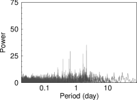
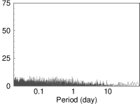
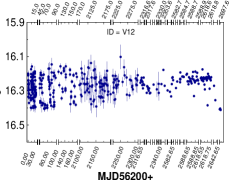
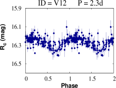
Figure 3: Top left panel : Lomb-Scargle power spectrum for the star V12. Top right panel : Power spectra of its shuffled LC. The highest peak at 2.3 days is taken as the estimated period. Bottom left panel : LC of the star V12. Data gaps are represented with vertical gaps along the axis. Bottom right panel : Phase-folded LC of the star V12 with the estimated period of 2.3 days.

In Figure 4 we show the RMS dispersion of all the target stars as a function of mean instrumental magnitude. The dispersion increases towards the fainter end due to the increase in photometric uncertainty. Identified variables are shown with blue open circles. Despite having a very high RMS value, some of the stars in Figure 4 are not designated as variables due to unusually high photometric errors (bad pixels, the bright background of the nearby star and residual from the cosmic corrections could be possible reasons) compared to the stars of the same magnitude bin. Once again these stars were visually checked to ascertain the variability.

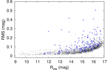
Figure 4: The RMS dispersion of instrumental magnitude as a function of mean instrumental magnitude of the stars in the Sh 2-190 region (black dots). Open circles are the identified variable stars.

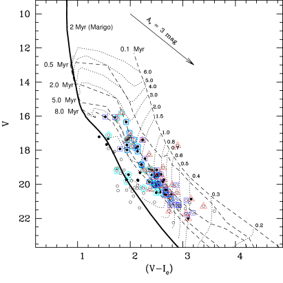
Figure 5: $V/(V-I_{c})$ CMD for the variable stars in the Sh 2-190 region. Filled and open circles represent periodic and non-periodic variables, respectively. Cyan pentagons represent variable stars with membership probability higher than 80% as derived from the PM data. Class ii and Class iii YSOs are plotted with red triangle and blue square symbols, respectively. The black thick curve shows the 2 Myr post-MS isochrone for the solar metallicity obtained from Marigo et al. (2008), while the black dashed and dotted curves represent the PMS isochrones for various ages and evolutionary tracks for various masses, respectively (Siess et al., 2000). All the isochrones and evolutionary tracks are corrected for the distance (2.1 kpc) and reddening (A${}_{V}=$ 2.46 mag). The arrow indicates the reddening vector.

By adopting the aforementioned procedure, we identified 134 variables (57 as periodic and 77 as non-periodic) from a sample of 3461 stars. Remaining stars are considered as non-variables in the present analysis. The period and amplitude of the variables range between 12 hrs-80 days and 0.1-2.2 mag, respectively. The catalogue by Panwar et al. (2017) has been used to cross-identify 85 variables as probable PMS stars. A 1-arcsec search radius was adopted for the cross identification. Thirty seven and forty eight PMS variables as per classification by Panwar et al. (2017) are found to be Class ii and Class iii sources, respectively. Almost half of the PMS variables (i.e., 45) are found to be periodic in nature and the rest have irregular brightness variation. The identification number, coordinates, period and other parameters of these PMS variables are listed in Table 3. The remaining 49 variables could be MS/field stars and their LC will be discussed in a separate study.

4.5 Determination of Physical Parameters of the variables

4.5.1 Through HR diagram

Figure 5 shows the $V/(V-I_{c})$ color-magnitude diagram (CMD) for all the identified variables along with the post-MS and PMS isochrones. We have detected variability down to a very deep magnitude limit of $V\sim 22$ mag. The Class  ii and Class  iii PMS variables are indicated by red triangle and blue square symbols, respectively. The location of the 36 variables identified as members of the Sh 2-190 region (cf. Section 4.2) are also shown with cyan pentagons in Figure 5. Clearly, almost all of the variables having counterparts in the published catalog of YSOs (Panwar et al., 2017) are located above the MS, as expected for PMS objects, on the CMD. With a few exceptions at fainter magnitudes where the parallax errors are high, a majority of the members also fall in the PMS phase. These confirm that our variables are in the PMS phase.

We have estimated the age and mass of each PMS variable from their position in the CMD (for details, cf. Chauhan et al., 2009; Sharma et al., 2017) and results are listed in the Table 3. Figure 6 shows the age and mass distribution of these PMS variables. The age distribution shows a peak around 3 Myr and an age spread of up to 6 Myr with some objects as old as 10 Myr. The average age and mass of the 85 PMS variables associated with Sh 2-190 are estimated to be $2.6\pm 1.5$ Myrs and $0.9\pm 0.6$ M_⊙, respectively.

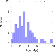
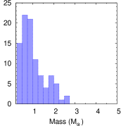
Figure 6: Age and mass frequency distribution for PMS variables.

4.5.2 Through Spectral energy distribution

To characterize and understand the physical nature of the PMS variables, we investigated their SEDs using the grid models and fitting tools of Whitney et al. (2003a, b, 2004) and Robitaille et al. (2006, 2007), respectively. This method has been widely used in our previous studies (e.g., Sinha et al., 2020; Sharma et al., 2020; Kaur et al., 2020; Pandey et al., 2020, and references therein). We fitted the SEDs of 84 PMS variables for which at least five band photometric data are available among the optical, NIR (2MASS) and MIR (WISE, $Spitzer$) data. The SED fitting tool fits each of the models to the data allowing the distance and extinction as free parameters. The input distance range of the IC 1805 region is taken as 1.9 - 2.3 kpc keeping in mind the error associated with distance estimation (see Section 4.3). As this region is highly nebulous, we varied the $A_{V}$ by putting foreground reddening of the IC 1805 region as a lower limit (2.5 mag). For the upper limit, we put a very large $A_{V}$ value, i.e., 30 mag, to accommodate embedded sources (See also, Sharma et al., 2017; Samal et al., 2012; Jose et al., 2013; Panwar et al., 2014). Instead of the formal errors in the catalog we set photometric uncertainties of 10% for the optical and 20% for both the NIR and MIR data to avoid any possible biases caused by underestimated flux uncertainties during fitting. We have used the relative probability distribution for the stages of all the ‘well-fit’ models to obtain the physical parameters of the PMS variables. The well-fit models for each source are defined by $\chi^{2}-\chi^{2}_{min}$ $\leq$ 2$N_{data}$, where $\chi^{2}_{min}$ is the goodness-of-fit parameter for the best-fit model and $N_{data}$ is the number of input data points.

In Figure 7, we show the sample SED for a PMS variable where the solid black curves represent the best fit and the grey curves are the subsequent good fits. From the well-fit models for each source derived from the SED fitting tool, we calculated the $\chi^{2}$ weighted model parameters such as mass, age, accretion rate, disc mass etc. of the PMS variables (see for details, Sinha et al., 2020) and are listed in Table 3. Here we would like to mention that the disc mass obtained from SED fitting may not account for all the mass of the circumstellar disc as we do not have photometric data that well covers all the disc extension emissions. Thus, this estimation could be a lower limit of the disc mass. The average age and mass of the 84 PMS variables are found to be $2.7\pm 1.6$ Myrs and $2.1\pm 1.2$ M_⊙, respectively. These parameters from the SEDs are comparable within errors to those obtained from the CMD ($2.6\pm 1.5$ Myrs and $0.9\pm 0.6$ M_⊙; cf. Section 4.5.1). These estimated physical parameters also indicate that the PMS variable are low mass T Tauri stars.

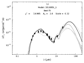
Figure 7: Sample SED of PMS variable created by the SED fitting tools of Robitaille et al. (2007). The black curve shows the best fit and the grey curves show the subsequent well fits. The filled circles with error bars denote the input flux values.

4.6 Disc indicators

We have used $\Delta(I_{c}-K_{s})$ and $([3.6]-[4.5])$ indices as disc indicators for the present study (for details, cf. Sinha et al., 2020). These color indices are sensitive to the inner and outer part of the stellar disc, respectively (Lada et al., 2000; Rodríguez-Ledesma et al., 2010). The index $\Delta(I_{c}-K_{s})$ is expressed as (cf. Hillenbrand et al., 1998):

$$\Delta(I_{c}-K_{s})=(I_{c}-K_{s})_{obs}-(A_{I_{c}}-A_{K_{s}})-(I_{c}-K_{s})_{0}$$ (2)

where $(I_{c}-K_{s})_{obs}$ is the observed color of the star, $(I_{c}-K_{s})_{0}$ is its intrinsic color and $A_{I_{c}}$ and $A_{K_{s}}$ are interstellar extinctions in the $I_{c}$ and $K_{s}$ bands, respectively. The extinction is normal towards this direction with A${}_{V}=$ 2.46 mag (Sagar & Yu, 1990; Hanson & Clayton, 1993; Joshi & Sagar, 1983; Straižys et al., 2013). The intrinsic color, $(I-K)_{0}$, were taken from the PMS isochrones of Siess et al. (2000).

4.7 X-ray luminosity

We converted the X-ray count rates provided in Townsley et al. (2014) of the identified PMS variables to the X-ray fluxes using the MEKAL model of PIMMS software. The required input parameters in this model are the temperature of the emitting coronal gas (kT), hydrogen column density ($N_{H}$) along the direction of the source and abundance of the PMS stars. We adopted a thermal plasma model with kT = 2.7keV and the abundance 0.4$\ast$Z_⊙, that are typical for PMS stars (Preibisch et al., 2005). The extinction value of A${}_{V}=$ 2.46 mag towards Sh 2-190 (cf. Section 4.3) yields a hydrogen column density $N_{H}$ = 5.48$\times$10²¹ cm^-2 (Güver & Özel, 2009). Finally, the PIMMS X-ray fluxes were corrected for a distance of 2.1 Kpc to get the $L_{X}$ of individual stars. The $L_{bol}$ of the PMS variables were taken from the PMS isochrones of Siess et al. (2000) according to their age and mass as derived by their CMD. The uncertainty in this approach could be due to potential differences in kT or A_V in individual stars.

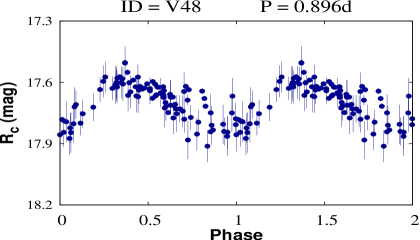
Figure 8: Phase folded LCs of 17 Class ii periodic variables. The identification numbers and periods (days) of the corresponding stars are given on the top of each panel. Complete set of LCs are provided in the electronic form only.

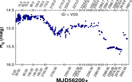
Figure 9: LCs of 20 Class ii non-periodic variables (CTTSs). When there are data gaps they are represented with vertical gaps along the axis. Corresponding identification numbers are given in each panel. A complete set of LCs are provided in the electronic form only.

5 Discussion

In this study, we will be focusing on the 85 identified PMS variables. We will discuss their LCs and the physical processes responsible for their variability in the ensuing sections.

5.1 Light curves of PMS variables

We will discuss and compare the LCs of 37 Class  ii and 48 Class  iii variables in the following sub-sections.

5.1.1 Class  ii variables

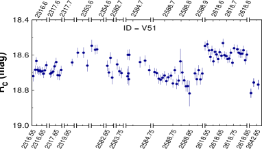
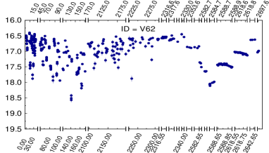
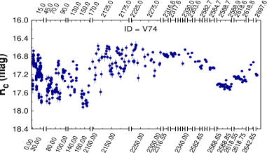
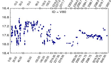
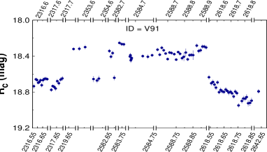
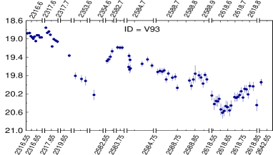
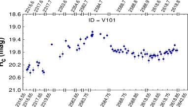
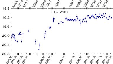
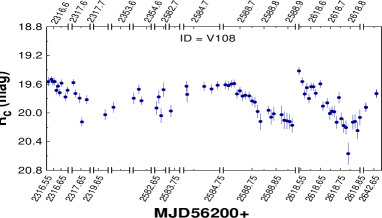
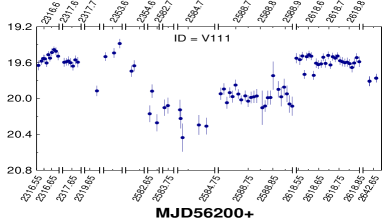
Figure 9: Contd.

The LCs of 17 Class ii periodic variables are shown in Figure 8. The period of these variables ranges from 0.9 days to 24 days with a median value of 3.1 days. Almost half of these variables have a period longer than 5 days. Longer periods are common in the stars with circumstellar disc (e.g., Edwards et al., 1993; Affer et al., 2013). The LCs of 20 non-periodic Class ii variables are shown in Figure 9. The amplitude of these variables ranges from 0.25 to 2.2 mag with a median value of 0.81 mag. Almost half of these variables have amplitude larger than 1 mag. In the LCs of V03 and V04, there are huge ($\sim$ 0.5-1.0 mag) dips indicative of occultation events that span for months. These occultation events are more sensitive at shorter wavelengths as can be seen in the Figure 10. Although there are large time gaps in some photometric bands, around MJD 2150+56200 and MJD 2588+56200 for V03 and around MJD 75+56200 and MJD 130+56200 days for V04, we note that as the star gets fainter their colors also become redder, which can be seen from both $V$-$I_{c}$ and $V$-$R_{c}$ colors. These events could be due to dust occultations. Apart from the occultation events, these LCs are mostly stable with some minute variations. In some other LCs (e.g., V08, V10, V62, V74 and V80) also, we see significant dips but due to lack of continuous data it is difficult to comment on their nature. In the cases of V62, V74 and V80, there are strong inter-day variations along with systematic increasing and decreasing trends at different epochs. The peak-to-trough amplitude of variations in these stars are $>$ 1.2 mag with V62 having 2.2 mag variation. V40, V51, V91 and V111 also show a daily variation of the “stochastic” nature, which may be caused by superposition of variable extinction and stochastic accretion (Cody et al., 2014). In contrast, V30, V31, V93, V101 and V107 show an increase or decrease in the brightness throughout or in some part of their LCs. The above mentioned characteristics are typical of CTTSs (e.g., Parks et al., 2014). These 20 Class ii non-periodic variables are thus further classified as CTTSs (see also, Bhardwaj et al., 2019). These classifications are given in Table 3.

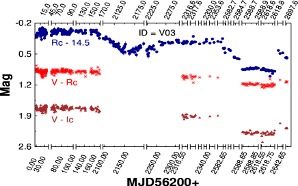
Figure 10: Color evolution of a few selected CTTSs variables. The R_c band LC, V-R_c and V-I_c color curves are shown with blue filled circle, red stars and brown triangles, respectively. When there are data gaps they are represented with vertical gaps along the axis. A complete set of LCs is provided in the electronic form only.

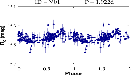
Figure 11: Phase folded LCs of 28 Class iii periodic variables (WTTSs). The identification numbers and periods (days) of the corresponding stars are given on the top of each panel. A complete set of LCs is provided in the electronic form only.

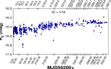
Figure 12: LCs of 20 Class iii non-periodic variables. When there are data gaps they are represented with vertical gaps along the axis. Corresponding identification numbers are given in each panel. A complete set of LCs are provided in the electronic form only.

5.1.2 Class  iii variables

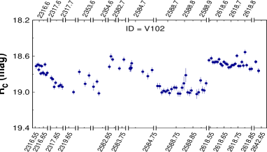
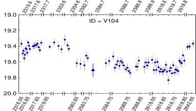
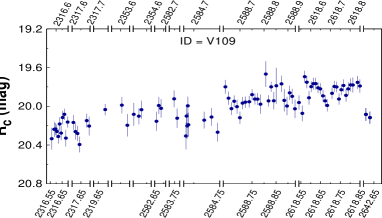
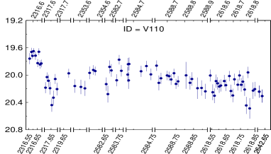
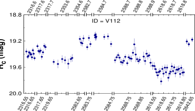
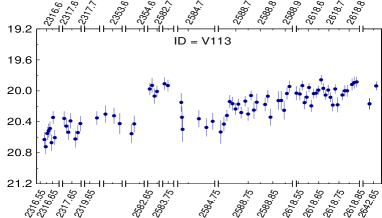
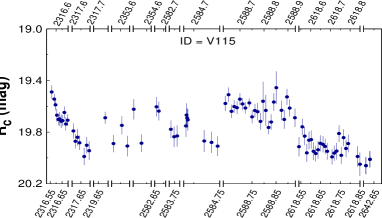
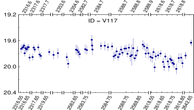
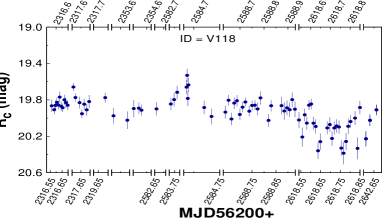
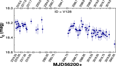
Figure 12: Contd.

The LCs of the 28 Class iii periodic variables are shown in the Figure 11. The period of these sources ranges between 0.5 days to 24 days with a median value of 1.6 days. Twenty one (75%) out of the twenty eight stars have period less than 5 days. The Class iii sources are showing amplitude variations in the range $\sim$0.1-0.7 mag and a majority of them (21 i.e., 75%) have amplitudes $<$ 0.4 mag. These characteristics are typical of WTTSs where variability is mostly caused by the irregular distribution of cool spots on the stellar surface. Hence, these 28 variables are further classified as WTTSs (see also, Bhardwaj et al., 2019). These classifications are given in Table 3. The LCs of the 20 non-periodic Class iii variables are shown in the Figure 12. Their amplitudes range from 0.26 to 1 mag with median value of 0.55 mag. More than 63% (i.e. 12) of these variables have amplitudes $\leq$ 0.7 mag.

5.1.3 Comparison between the light curves of Class  ii and Class  iii variables

From the previous sub-sections, it is evident that Class ii sources have in general a longer period as compared to the Class iii sources. Class iii sources are more evolved and have less disc material around these stars. According to the disc-locking model, this allows Class iii sources to spin-up freely without any regulation imposed by the disc (Koenigl, 1991; Shu et al., 1994).

The strength of the flux variation depends on the related physical mechanism. The flux variations in Class ii and Class iii objects are mostly governed by the disc phenomenon (accretion, extinction etc.) and spot modulation, respectively. In general, these different mechanisms cause the Class ii objects to vary with larger amplitude relative to the Class iii objects. In our sample, the amplitude in Class ii sources ranges from 0.18 to 2.2 mag with a median 0.58 mag while Class iii sources have amplitudes in the range 0.11 to 1.0 mag with a median amplitude 0.36 mag. To statistically verify whether the Class ii and Class iii objects differ in terms of their variability amplitude, we plotted the normalized cumulative amplitude distribution of these sources in Figure 13. The figure manifests that Class ii variables have larger amplitudes of variation as compared to the Class iii sources with 99% confidence level as calculated by the Kolmogorov-Smirnov test. Similar trends have been found previously for the variables identified in the IC 5070 (Bhardwaj et al., 2019) and Sh 2-170 (Sinha et al., 2020) star-forming regions. Also, the LCs of Class ii variables show more dynamic and different temporal features which include either a single or a combination of the phenomenon like short duration fadings, long term dippers induced by circumstellar extinctions, sharp increases in luminosity (bursters) and stochastic changes in brightness caused by variable accretion (Cody et al., 2014).

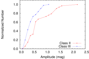
Figure 13: Normalized cumulative amplitude distribution of Class ii and Class iii variables.

5.2 Role of disc in stellar variability

Edwards et al. (1993) have found that stars with longer periods are surrounded by an accretion disc while the stars lacking accretion disc are predominantly fast rotators. This distribution can be explained if the stellar angular momentum is regulated during the disc accretion phase by a mechanism that balances the spin-up torque applied by the accretion of high angular momentum material from the disc. The magnetic star-disc interaction between the stellar magnetosphere and the circumstellar disc has been proposed to explain this effective removal of angular momentum from PMS stars during the first $\sim$ 10 Myr of their evolution (i.e., disc-locking, Koenigl, 1991; Shu et al., 1994; Najita, 1995; Ostriker & Shu, 1995).

The disc-locking mechanism can be verified from the bimodal distribution of variability period in young stars as the disc-locked slow rotators can explain the separate period distribution from the usual ones (Koenigl, 1991; Shu et al., 1994). However, there have been several conflicting pieces of evidence regarding this, for example, some authors (e.g., Herbst et al., 2002; Lamm et al., 2005; Sinha et al., 2020) have found the bimodal period distribution which favors the disc-locking mechanism, while others (Makidon et al., 2004) have found the unimodal period distribution. To further test this mechanism, in Figure 14, we show the period distribution for all 45 periodic PMS variables (with 17 Class iii and 28 Class iii sources presented separately on the right) identified in the Sh 2-190 region. Although the distribution looks unimodal for all the periodic PMS variables, we can see different period distributions for the Class ii and Class iii sources. While the Class iii sources show a peak period of around 1 day, the Class ii sources have a peak of around 3 days. Besides the small number of stars in the sample, we have performed Kolmogorov-Smirnov (KS) test to the period distribution of the Class ii and Class iii objects. It returned a $p$-value of 0.16 indicating that the probability of these objects representing different population is 84%. Longer periods for the younger objects hint towards the disc-locking mechanism. A statistically significant sample of objects is required to draw a definitive conclusion.

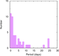
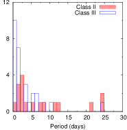
Figure 14: Left panel: Period distribution of all periodic PMS variables. Right panel: Period distribution of Class ii and Class iii variables.

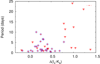
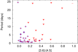
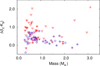
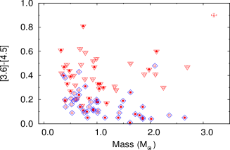
Figure 15: Upper panels : Period as a function of NIR excess $\Delta(I_{c}-K_{s})$ & MIR excess $[[3.6]-[4.5]]$ Lower panels : NIR excess $\Delta(I_{c}-K_{s})$ and MIR excess $[[3.6]-[4.5]]$ as a function of stellar mass. The Class ii and Class iii sources are represented with inverted triangles and diamonds, respectively. Filled and open circles represent periodic and non-periodic variables, respectively. Corresponding mean errors are shown with error bars.

The disc-locking mechanism can be further verified from the correlation between rotation period and size of the disc of PMS variables (Herbst et al., 2002). In Figure 15 (upper panels), we plot rotation periods as a function of the disc indicators $\Delta(I_{c}-K_{s})$ and $[[3.6]-[4.5]]$ (see Section 4.6). Although we do not see any clear trends in these plots but they roughly suggest that the mean rotational speed becomes less when there is a increase in NIR/MIR excess. The period versus $\Delta(I_{c}-K_{s})$ plot suggest that most of the slow rotators (having periods $>$ 10 days) are Class ii sources having higher value of $\Delta(I_{c}-K_{s})$ index ($>$ 0.75 mag), whereas Class iii sources with $\Delta(I_{c}-K_{s})$ $\sim$ 0.3 mag have periods $\leqslant$ 10 days. Similar results have also been found previously for different regions (e.g., Herbst et al., 2000, 2002; Lamm et al., 2005; Rebull et al., 2006; Sinha et al., 2020). Besides the small number of the periodic stars, these results suggest that the presence of a disc regulates stellar rotation in a way that the younger stars having a thicker disc are slow rotators. To check the mass dependence of $\Delta(I_{c}-K_{s})$ and $[[3.6]-[4.5]]$ indices, we plot these parameters in the lower panels of Figure 15. Although we need more data points to conclude, but it appears that the higher mass stars have relatively lesser IR excess than the lower mass stars.

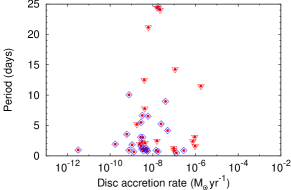
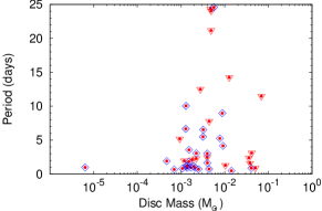
Figure 16: Period as a function of disc accretion rate and disc mass. The symbols are the same as in Figure 15.

Since, in PMS stellar evolution, mass accretion takes place from the circumstellar disc on to the star (Shu et al., 1994; Lamm et al., 2005), the rotation of stars with active accretion is likely to be more regulated by the disc and they have longer period as compared to disc-less stars where accretion is inactive. We plot period as a function of disc accretion rate and disc mass of the PMS variables in Figure 16. Though we do not see any dependence of rotation period on the disc mass or disc accretion rate a lager sample of PMS variables will be helpful to conclude on this. For a given rotation period, the value of disc mass and accretion rate spans over few orders of magnitude. Previous authors (for example, Fallscheer & Herbst, 2006; Venuti et al., 2017) have investigated any possible correlation between rotation period and accretion rate using the UV excess as an indicator of accretion and found that slowly rotating stars are more likely to have lager UV excess. Venuti et al. (2017) found that CTTSs with large UV excess are mostly slow rotators while WTTSs are distributed over the whole period range and have smaller UV excess. When comparing the accretion rate of the CTTSs with their rotation period they found a diverse range of accretion values corresponding to a rotation period and speculated that different sets of mechanisms are responsible for regulating stellar rotation and accretion rates. While the accretion rate is regulated by the small scale magnetic field structure near the stellar surface, star-disc coupling and angular momentum regulation is dominated by the large-scale magnetic field structure (Gregory et al., 2012).

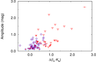
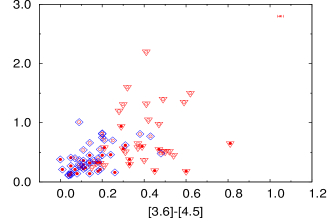
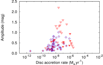
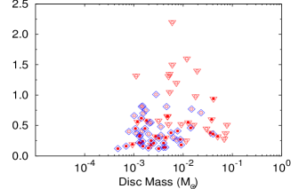
Figure 17: Amplitude of variation as a function of NIR excess $\Delta(I_{c}-K_{s})$ and MIR excess $[[3.6]-[4.5]]$ (upper panels) and as a function of disc accretion rate and disc mass (lower panels). The symbols are the same as in Figure 15.

As the variable accretion and extinction by circumstellar disc significantly enhance the brightness variation in PMS stars, the presence of thicker disc and active accretion are also expected to influence the amplitude of brightness variation. The amplitude of variation as a function of $\Delta(I_{c}-K_{s})$ and $[[3.6]-[4.5]]$ are plotted in the upper panels of Figure 17. Clearly, the amplitude of variation increases with disc indicators, which means the presence of thicker disc and envelop induces larger amplitude variations. The plots also show that the Class ii sources have active circumstellar discs as compared to Class iii sources. Lower panels of the Figure 17 suggest that the stars with higher disc accretion activity ($>10^{-8}$ M${}_{\odot}~{}yr^{-1}$) induces higher amplitude of variation. The amplitude of variation also seems to depends on the mass of the circumstellar disc in the sense that stars having discs with mass $\geqslant$ 2$\times 10^{-3}$ M_⊙ show larger amplitude of variation as compared to those with lower disc mass. Hence, it appears that the Class ii sources exhibit more active and dynamic variability because of their accretion activities. Herbst et al. (2002) have also reported a good correlation of RMS amplitude with $\Delta(I_{c}-K_{s})$ in Orion Nebula Cluster. Similar results were also found in our previous studies on Sh 2-170 (Sinha et al., 2020).

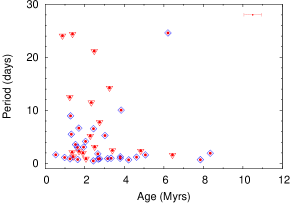
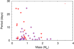
Figure 18: Period as a function of age and mass of PMS variables. Corresponding mean errors are shown with error bars in the top right corner of each panel. The symbols are the same as in Figure 15.

5.3 Dependence of stellar variability on the age and mass of stars

The age and mass of PMS stars are very important parameters that constrain the physical processes of the evolution of the central star and the circumstellar disc. The rate of the mass-accretion usually depends on the initial mass of the PMS stars. During the evolution, PMS stars also increase their mass through the accretion of material from the circumstellar disc. The disc subsequently dissipates resulting fewer activities related to accretion processes. To understand the role of age and mass on stellar variability, we plotted the period and amplitude of the PMS variables as a function of their age and mass in Figure 18 and Figure 19, respectively. The upper panel of Figure 18 indicates that stars with periods up to $\sim$4 days are uniformly distributed over the entire range of ages, whereas most of the PMS variables having periods $>$ 4 days are younger than $\sim$4 Myr. Lata et al. (2016) have also reported a similar result that PMS stars with age $\geqslant$ 3 Myr are relatively fast rotators.

The lower panel of Figure 18 displays the dependence of period on the stellar mass. Here also we can see a decreasing trend in the distribution, i.e, out of 12 rotators having period $>$ 6 days, 11 have mass $<$ 1.2 M_⊙, whereas all the stars more massive than $>$ 1.2 M_⊙ are fast rotators (period $<$ 6 days). Previously, Roquette et al. (2017) and Henderson & Stassun (2012) have found that the PMS stars with mass roughly below 0.5 M_⊙ rotate slower than their massive counterparts in their study related with CygOB2 and NGC 6530 regions, respectively. On the contrary, Littlefair et al. (2010) have found that the lower mass stars ($<$ 0.4 M_⊙) rotate relatively faster than the higher mass stars ($>$ 0.4 M_⊙) in the CepOB3 region. Venuti et al. (2017) have also found similar result in the case of NGC 2264. They divided the stars in three mass bins i.e., (i) M $<$ 0.4 M_⊙; (ii) 0.4 M_⊙ $\leq$ M $\leq$ 1 M_⊙; (iii) M $>$ 1 M_⊙, and found that lowest mass group consists a peak of fast rotators (P $=$ 1-2 days) while for higher mass groups an emerging peak around P $=$ 3-4 days are seen. Stars more massive than 1.4 M_⊙ rotate faster as they have largely radiative interiors unlike their less massive counterparts which spend long time along the convective track during their PMS evolution. Convection brakes the star by powering stellar winds that carry angular momentum. Massive stars lack this mechanism and experience different rotational evolution from less massive stars. To check whether this effect is present in NGC 2264, Venuti et al. (2017) further divided their 3rd mass group into below and above 1.4 M_⊙ and found that the latter rotate faster with a median period of 3 days while the stars in the former group are slow rotators with median period of 5 days. In the present study, we also observe that the higher mass stars (M $>$ 1.2 M_⊙) are fast rotators. Recently, Sinha et al. (2020) and Lata et al. (2012, 2016) have also found similar results. Herbst et al. (2000) and Littlefair et al. (2005) have also found strong correlation between stellar mass and rotation rate in the case of ONC and IC 348, respectively. Littlefair et al. (2005) concluded that the strong mass dependence of rotation period seen in ONC (Herbst et al., 2002) may well be a common feature of PMS populations.

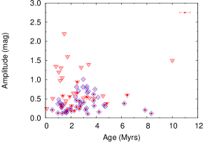
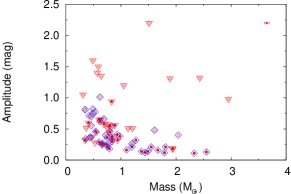
Figure 19: Amplitude of variations as a function of age and mass of PMS variables. The symbols are the same as in Figure 15. Corresponding mean errors are shown with error bars.

Since younger stars should have higher disc fraction, we may see a larger amplitude variation in the younger population. In the top panel of Figure 19, we can observe a decrease in the amplitude of the PMS variables with the increase in their age. The decreasing trend with age supports previous findings (Lata et al., 2011, 2012, 2016; Sinha et al., 2020) that a significant amount of disc is dissipated by $\sim$ 5 Myr. This is also in accordance with the result obtained by Haisch et al. (2001). The bottom panel shows amplitude as a function of stellar mass. Although the trend is not clear in the case of Class ii objects but it appears that the amplitude of variation decreases with increase in the mass of Class iii objects (blue diamonds). This result seems to indicate that relatively massive PMS stars have smaller spots on their surface. As the variability in Class iii sources (or WTTSs) sources are mostly regulated by cool spots on their photosphere the size of the spot is proportional to amplitude of variation. With increasing mass a star develops a larger radiative core and the convective envelope becomes thinner, causing less efficient dynamo mechanism, and consequently the spot size reduces (Thomas & Weiss, 2008; Strassmeier, 2009).

5.4 X-ray activities in PMS stars

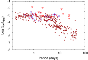
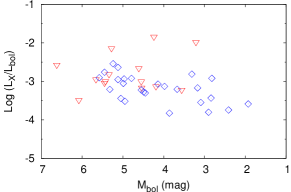
Figure 20: Fractional X-ray luminosity of the periodic PMS sources as a function of period (top panel) and bolometric magnitude (bottom panel). The brown square symbols in the upper panel represent the MS samples taken from Pizzolato et al. (2003). Other symbols are the same as in Figure 15.

.

Both accreting and non-accreting PMS stars exhibit strong X-ray emission produced mainly by magnetic activity in hot corona while an additional soft component is produced by accretion shock in the case of accreting stars. The magnetic activity is believed to be generated by a dynamo mechanism at the interface of the radiative and convective zones that is driven by rotational and convective motions ($\alpha~{}\Omega$ dynamo: Parker, 1955). For the MS stars, it is found that X-ray luminosity increases with increasing rotation speed until a star reaches a saturation level (log ($L_{X}/L_{bol}$) $\approx$ -3, Pizzolato et al., 2003). However, the period-magnetic activity relation in PMS stars is not well established. To explore this, we have plotted fractional X-ray luminosity, i.e., ($L_{X}/L_{bol}$), as a function of rotation period of PMS stars in the upper panel of Figure 20. The distribution is roughly flat at the saturation level, log ($L_{X}/L_{bol}$) = -3.05. This is comparable with the saturation value of the MS sample of Pizzolato et al. (2003) shown with brown square symbols in the plot. Alexander & Preibisch (2012) have found similar results in IC348 and concluded that more or less chaotic nature of convective dynamo is responsible for large scatter in magnetic activity among TTSs. The scatter of $L_{X}/L_{bol}$ in Figure 20 is similar to that of IC348 which shares a similar age with IC 1805 ($\approx$ 3 Myrs). On the other hand, Orion which is younger ($\approx$ 1 Myrs) shows a similar distribution with a larger scatter of $L_{X}/L_{bol}$ (see also, Alexander & Preibisch, 2012). In case of NGC 6530, Henderson & Stassun (2012) have found fractional X-ray luminosities of the stars are more or less flat with rotation period, approximately at the saturation level. However, the fastest rotators show lower X-ray luminosities, suggestive of the so-called “super-saturation” where X-ray luminosity decreases with increasing rotation speed.

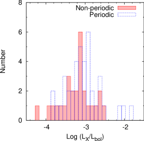
Figure 21: Distribution of log ($L_{X}/L_{bol}$) of periodic (blue bordered histogram) and non-periodic (red shaded histogram) PMS stars.

To check the dependence of X-ray activity on stellar mass we have plotted fractional X-ray luminosity as a function of bolometric magnitude ($M_{bol}$) in the lower panel of Figure 20. Although it is difficult to conclude from this small sample size, it appears that there is a weak anti-correlation for the Class iii objects in the sense that $L_{X}/L_{bol}$ decreases as the stars get brighter or massive. This suggests that lower mass stars, which are mostly convective, produce a larger fraction of X-ray in comparison to their massive counterparts. More studies on larger sample size are required to confirm this result.

We have also explored the possibility if there is any difference in the X-ray activity of PMS stars with (periodic) and without (non-periodic) rotation period. The distribution of log ($L_{X}/L_{bol}$) of the periodic and non-periodic PMS stars are shown with blue-bordered and red shaded histograms, respectively in Figure 21. The distribution of periodic PMS stars peaks at a larger value of $L_{X}/L_{bol}$ relative to non-periodic PMS stars. The average values of the fractional X-ray luminosity ($L_{X}/L_{bol}$) in periodic stars (0.17$\pm$0.28%) is almost double as compared to non-periodic (0.09$\pm$0.07%) stars. In our sample of WTTSs and CTTSs (cf. Section 5.1), the former (mean $L_{X}/L_{bol}$ = 0.09$\pm$0.07%) are also found to be more X-ray active than the latter (mean $L_{X}/L_{bol}$ = 0.04$\pm$0.03%). This may be due to the fact that the rapid stellar rotation in the later stage of stellar evolution produces a stronger magnetic field through an $\alpha~{}\Omega$ type dynamo (for stars with radiative core and convective envelope) or through a distributed turbulent dynamo (for fully convective stars) (Stassun et al., 2004).

6 Summary and conclusion

In this paper we have presented the results of the multi-epoch and deep imaging survey in $V$, $R_{c}$, $I_{c}$ bands to understand the characteristics of PMS variables in the Sh2-190 region. Following are the main results.

• We have identified 134 variables in this region. Eighty-five of them are found to be probable PMS stars, whereas the remaining stars could be MS/field population. Out of the 85 PMS variables, 37 and 48 are classified as Class ii and Class iii sources, respectively. LCs of 17 Class ii and 28 Class iii variables show periodicity.

• The majority of the PMS variables have mass and age in the range of 0.1 $\leq$ M/M_⊙ $\leq$ 4.0 and 0.3 - 2.0 Myrs, respectively, and hence should be TTSs. The rotation period of the PMS variables ranges from 12 hrs to 24 days, whereas the amplitude of variation spans from 0.1 mag to 2.2 mag. The amplitude is larger in Class ii sources (up to 2.2 mag) as compared to Class iii sources (upto $\sim$ 1.0 mag).

• In general,it appears that Class ii sources show longer period of variability as compared to Class iii sources. Also, the period distribution of Class ii sources peaks at $\sim$ 3 days, while Class iii sources peak at 1 day. Stars with smaller IR excess seem to rotate faster in comparison to stars with larger IR excess.

• The amplitude of variation in the PMS stars shows a increasing trend with increase in the disc indicators. This suggests that Class ii sources with circumstellar disc exhibit more active and dynamic activities as compared to Class iii sources. The amplitude of variability seems to be influenced by disc mass and disc accretion rate in the sense that the presence of massive discs ($\gtrsim$ 2 $\times 10^{-3}$ M_⊙) and higher disc accretion rate ($\gtrsim 10^{-8}$ M${}_{\odot}yr{{}^{-1}}$) induces higher amplitude of variation.

• The different period distribution of Class ii and Class iii sources and the dependence of rotation period on IR excess are compatible with the ‘disc-locking’ model. This model suggests that the rotation of PMS stars is regulated by the presence of circumstellar discs, that when a star is disc-locked, its rotation speed doesn’t change and that when the star is released from the locked-up disc, it can spin up with its contraction.

• With the increase in stellar mass in the range of $\sim$0.5-2.5 M_⊙ the period of PMS variables decreases. The amplitude of variation of the Class iii objects show a decreasing trend with increasing mass. This suggests that with increasing mass a star develops the radiative core quickly and convective envelope becomes thinner, which results in the reduction in spot size and causes lesser amplitude of variation in stars whose variability is regulated by spot modulation.

• These results favor the preposition that cool spots on WTTSs are mostly responsible for their variations, while hot spots on CTTSs caused by variable mass accretion from the inner disc and/or variable extinction events contribute to their larger amplitudes and more irregular behaviors.

• Fractional X-ray luminosity ($L_{X}/L_{bol}$) as a function of rotation period shows a flat distribution at log ($L_{X}/L_{bol}$) $\approx$ -3.0, which indicates that PMS stars in the Sh 2-190 region are at the saturation level reported for the MS stars. The log ($L_{X}/L_{bol}$) of younger Class  ii sources is generally less as compared to that of comparatively older Class  iii sources hinting towards a less significant role of the stellar disc-related mechanisms in X-ray generation.

1 Figures to be published in electronic form only

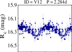
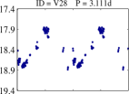
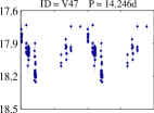
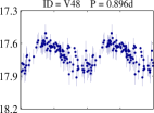
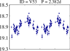
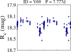
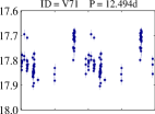
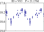
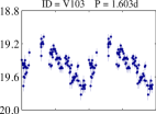
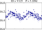
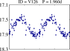
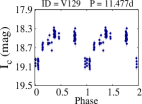
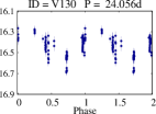
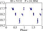
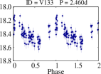
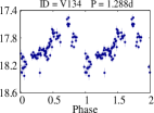
Figure 8: Phase folded LCs of 17 Class ii periodic variables. The identification numbers and periods (days) of the corresponding stars are given on the top of each panel.

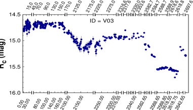
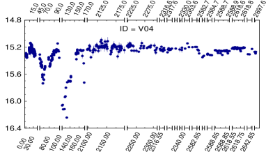
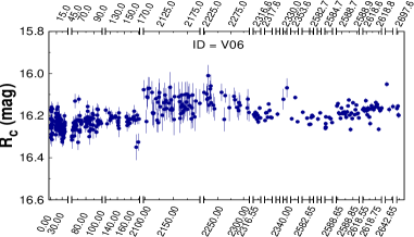
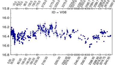
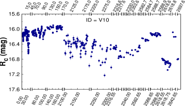
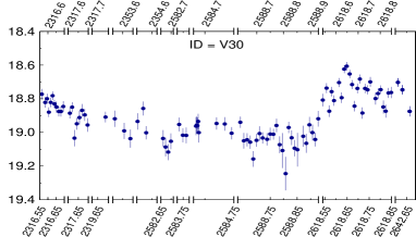
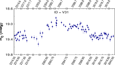
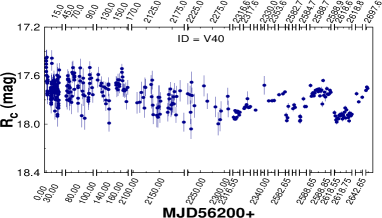
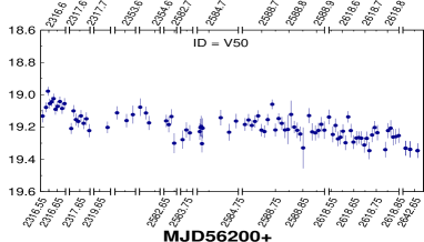
Figure 9: LCs of 20 Class ii non-periodic variables (CTTSs). When there are data gaps they are represented with vertical gaps along the axis. Corresponding identification numbers are given in each panel.

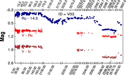
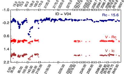
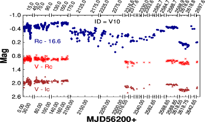
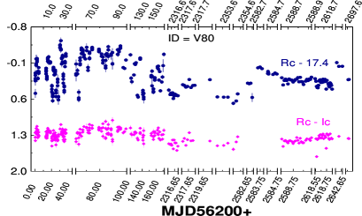
Figure 10: Color evolution of a few selected CTTSs variables. The R_c band LC, V-R_c, V-I_c and R_c-I_c color curves are shown with blue filled circle, red stars, brown triangles and magenta diamonds, respectively. When there are data gaps they are represented with vertical gaps along the axis.

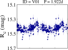
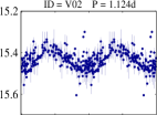
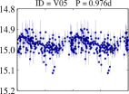
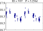
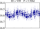
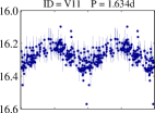
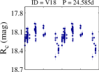
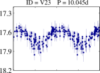
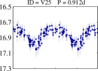
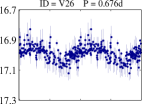
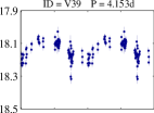
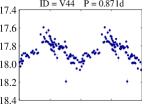
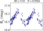
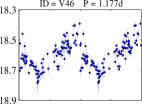
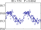
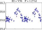
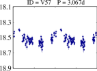
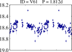
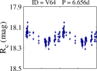
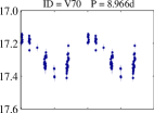
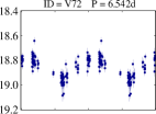
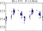
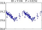
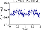
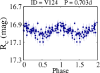
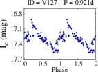
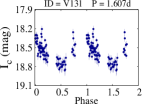
Figure 11: Phase folded LCs of 28 Class iii periodic variables (WTTSs). The identification numbers and periods (days) of the corresponding stars are given on the top of each panel.

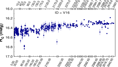
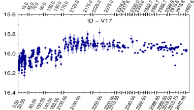
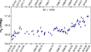
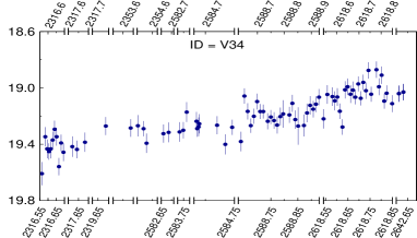
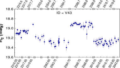
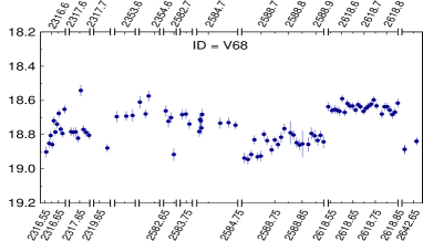
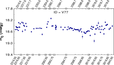
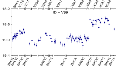
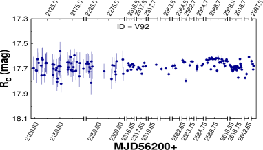
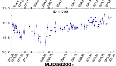
Figure 12: LCs of 20 Class iii non-periodic variables. When there are data gaps they are represented with vertical gaps along the axis. Corresponding identification numbers are given in each panel. A complete set of LCs are provided in the electronic form only.

References

- Affer et al. (2013) Affer, L., Micela, G., Favata, F., Flaccomio, E., & Bouvier, J. 2013, MNRAS, 430, 1433, doi: 10.1093/mnras/stt003
- Alencar et al. (2010) Alencar, S. H. P., Teixeira, P. S., Guimarães, M. M., et al. 2010, A&A, 519, A88, doi: 10.1051/0004-6361/201014184
- Alexander & Preibisch (2012) Alexander, F., & Preibisch, T. 2012, A&A, 539, A64, doi: 10.1051/0004-6361/201118100
- Bailer-Jones et al. (2018) Bailer-Jones, C. A. L., Rybizki, J., Fouesneau, M., Mantelet, G., & Andrae, R. 2018, AJ, 156, 58, doi: 10.3847/1538-3881/aacb21
- Balaguer-Núnez et al. (1998) Balaguer-Núnez, L., Tian, K. P., & Zhao, J. L. 1998, A&AS, 133, 387, doi: 10.1051/aas:1998324
- Banse et al. (1992) Banse, K., Grosbol, P., & Baade, D. 1992, in Astronomical Society of the Pacific Conference Series, Vol. 25, Astronomical Data Analysis Software and Systems I, ed. D. M. Worrall, C. Biemesderfer, & J. Barnes, 120
- Bhardwaj et al. (2019) Bhardwaj, A., Panwar, N., Herczeg, G. J., Chen, W. P., & Singh, H. P. 2019, A&A, 627, A135, doi: 10.1051/0004-6361/201935418
- Bouvier et al. (2013) Bouvier, J., Grankin, K., Ellerbroek, L. E., Bouy, H., & Barrado, D. 2013, A&A, 557, A77, doi: 10.1051/0004-6361/201321389
- Bouvier et al. (2007) Bouvier, J., Alencar, S. H. P., Boutelier, T., et al. 2007, A&A, 463, 1017, doi: 10.1051/0004-6361:20066021
- Carney et al. (2016) Carney, M. T., Yıldız, U. A., Mottram, J. C., et al. 2016, A&A, 586, A44, doi: 10.1051/0004-6361/201526308
- Chauhan et al. (2009) Chauhan, N., Pandey, A. K., Ogura, K., et al. 2009, MNRAS, 396, 964, doi: 10.1111/j.1365-2966.2009.14756.x
- Cody & Hillenbrand (2010) Cody, A. M., & Hillenbrand, L. A. 2010, ApJS, 191, 389, doi: 10.1088/0067-0049/191/2/389
- Cody et al. (2014) Cody, A. M., Stauffer, J., Baglin, A., et al. 2014, AJ, 147, 82, doi: 10.1088/0004-6256/147/4/82
- Cutri et al. (2003) Cutri, R. M., Skrutskie, M. F., van Dyk, S., et al. 2003, VizieR Online Data Catalog, 2246
- Edwards et al. (1993) Edwards, S., Strom, S. E., Hartigan, P., et al. 1993, AJ, 106, 372, doi: 10.1086/116646
- Fallscheer & Herbst (2006) Fallscheer, C., & Herbst, W. 2006, ApJ, 647, L155, doi: 10.1086/507525
- Fritzewski et al. (2016) Fritzewski, D. J., Kitze, M., Mugrauer, M., et al. 2016, MNRAS, 462, 2396, doi: 10.1093/mnras/stw1797
- Grankin et al. (2008) Grankin, K. N., Bouvier, J., Herbst, W., & Melnikov, S. Y. 2008, A&A, 479, 827, doi: 10.1051/0004-6361:20078476
- Greene et al. (1994) Greene, T. P., Wilking, B. A., Andre, P., Young, E. T., & Lada, C. J. 1994, ApJ, 434, 614, doi: 10.1086/174763
- Gregory et al. (2012) Gregory, S. G., Donati, J. F., Morin, J., et al. 2012, ApJ, 755, 97, doi: 10.1088/0004-637X/755/2/97
- Guo et al. (2018) Guo, Z., Herczeg, G. J., Jose, J., et al. 2018, ApJ, 852, 56, doi: 10.3847/1538-4357/aa9e52
- Güver & Özel (2009) Güver, T., & Özel, F. 2009, MNRAS, 400, 2050, doi: 10.1111/j.1365-2966.2009.15598.x
- Haisch et al. (2001) Haisch, Karl E., J., Lada, E. A., & Lada, C. J. 2001, ApJ, 553, L153, doi: 10.1086/320685
- Hanson & Clayton (1993) Hanson, M. M., & Clayton, G. C. 1993, AJ, 106, 1947, doi: 10.1086/116775
- Henderson & Stassun (2012) Henderson, C. B., & Stassun, K. G. 2012, ApJ, 747, 51, doi: 10.1088/0004-637X/747/1/51
- Herbig & Bell (1988) Herbig, G. H., & Bell, K. R. 1988, Third Catalog of Emission-Line Stars of the Orion Population : 3 : 1988
- Herbst et al. (2002) Herbst, W., Bailer-Jones, C. A. L., Mundt, R., Meisenheimer, K., & Wackermann, R. 2002, A&A, 396, 513, doi: 10.1051/0004-6361:20021362
- Herbst et al. (2007) Herbst, W., Eislöffel, J., Mundt, R., & Scholz, A. 2007, Protostars and Planets V, 297
- Herbst et al. (1994) Herbst, W., Herbst, D. K., Grossman, E. J., & Weinstein, D. 1994, AJ, 108, 1906, doi: 10.1086/117204
- Herbst et al. (2000) Herbst, W., Maley, J. A., & Williams, E. C. 2000, AJ, 120, 349, doi: 10.1086/301430
- Hillenbrand (2002) Hillenbrand, L. A. 2002, arXiv Astrophysics e-prints
- Hillenbrand et al. (1998) Hillenbrand, L. A., Strom, S. E., Calvet, N., et al. 1998, AJ, 116, 1816, doi: 10.1086/300536
- Jose et al. (2013) Jose, J., Pandey, A. K., Samal, M. R., et al. 2013, MNRAS, 432, 3445, doi: 10.1093/mnras/stt700
- Joshi & Sagar (1983) Joshi, U. C., & Sagar, R. 1983, JRASC, 77, 40
- Joy (1945) Joy, A. H. 1945, ApJ, 102, 168, doi: 10.1086/144749
- Kaur et al. (2020) Kaur, H., Sharma, S., Dewangan, L. K., et al. 2020, ApJ, 896, 29, doi: 10.3847/1538-4357/ab9122
- Koenigl (1991) Koenigl, A. 1991, ApJ, 370, L39, doi: 10.1086/185972
- Lada et al. (2000) Lada, C. J., Muench, A. A., Haisch, Jr., K. E., et al. 2000, AJ, 120, 3162, doi: 10.1086/316848
- Lamm et al. (2004) Lamm, M. H., Bailer-Jones, C. A. L., Mundt, R., Herbst, W., & Scholz, A. 2004, A&A, 417, 557, doi: 10.1051/0004-6361:20035588
- Lamm et al. (2005) Lamm, M. H., Mundt, R., Bailer-Jones, C. A. L., & Herbst, W. 2005, A&A, 430, 1005, doi: 10.1051/0004-6361:20040492
- Lata et al. (2012) Lata, S., Pandey, A. K., Chen, W. P., Maheswar, G., & Chauhan, N. 2012, MNRAS, 427, 1449, doi: 10.1111/j.1365-2966.2012.22070.x
- Lata et al. (2011) Lata, S., Pandey, A. K., Maheswar, G., Mondal, S., & Kumar, B. 2011, MNRAS, 418, 1346, doi: 10.1111/j.1365-2966.2011.19582.x
- Lata et al. (2016) Lata, S., Pandey, A. K., Panwar, N., et al. 2016, MNRAS, 456, 2505, doi: 10.1093/mnras/stv2800
- Lenz & Breger (2005) Lenz, P., & Breger, M. 2005, Communications in Asteroseismology, 146, 53, doi: 10.1553/cia146s53
- Littlefair et al. (2005) Littlefair, S. P., Naylor, T., Burningham, B., & Jeffries, R. D. 2005, MNRAS, 358, 341, doi: 10.1111/j.1365-2966.2005.08737.x
- Littlefair et al. (2010) Littlefair, S. P., Naylor, T., Mayne, N. J., Saunders, E. S., & Jeffries, R. D. 2010, MNRAS, 403, 545, doi: 10.1111/j.1365-2966.2010.16066.x
- Lomb (1976) Lomb, N. R. 1976, Ap&SS, 39, 447, doi: 10.1007/BF00648343
- Loomis et al. (2017) Loomis, R. A., Öberg, K. I., Andrews, S. M., & MacGregor, M. A. 2017, ApJ, 840, 23, doi: 10.3847/1538-4357/aa6c63
- Makidon et al. (2004) Makidon, R. B., Rebull, L. M., Strom, S. E., Adams, M. T., & Patten, B. M. 2004, AJ, 127, 2228, doi: 10.1086/382237
- Marigo et al. (2008) Marigo, P., Girardi, L., Bressan, A., et al. 2008, A&A, 482, 883, doi: 10.1051/0004-6361:20078467
- Masci et al. (2019) Masci, F. J., Laher, R. R., Rusholme, B., et al. 2019, PASP, 131, 018003, doi: 10.1088/1538-3873/aae8ac
- McGinnis et al. (2015) McGinnis, P. T., Alencar, S. H. P., Guimarães, M. M., et al. 2015, A&A, 577, A11, doi: 10.1051/0004-6361/201425475
- Najita (1995) Najita, J. 1995, in Revista Mexicana de Astronomia y Astrofisica Conference Series, Vol. 1, Revista Mexicana de Astronomia y Astrofisica Conference Series, ed. S. Lizano & J. M. Torrelles, 293
- Ostriker & Shu (1995) Ostriker, E. C., & Shu, F. H. 1995, ApJ, 447, 813, doi: 10.1086/175920
- Pandey et al. (2020) Pandey, R., Sharma, S., Panwar, N., et al. 2020, ApJ, 891, 81, doi: 10.3847/1538-4357/ab6dc7
- Panwar et al. (2014) Panwar, N., Chen, W. P., Pandey, A. K., et al. 2014, MNRAS, 443, 1614, doi: 10.1093/mnras/stu1244
- Panwar et al. (2017) Panwar, N., Samal, M. R., Pandey, A. K., et al. 2017, MNRAS, 468, 2684, doi: 10.1093/mnras/stx616
- Parker (1955) Parker, E. N. 1955, ApJ, 122, 293, doi: 10.1086/146087
- Parks et al. (2014) Parks, J. R., Plavchan, P., White, R. J., & Gee, A. H. 2014, ApJS, 211, 3, doi: 10.1088/0067-0049/211/1/3
- Peeters et al. (2004) Peeters, E., Spoon, H. W. W., & Tielens, A. G. G. M. 2004, ApJ, 613, 986, doi: 10.1086/423237
- Pizzolato et al. (2003) Pizzolato, N., Maggio, A., Micela, G., Sciortino, S., & Ventura, P. 2003, A&A, 397, 147, doi: 10.1051/0004-6361:20021560
- Preibisch et al. (2005) Preibisch, T., Kim, Y.-C., Favata, F., et al. 2005, ApJS, 160, 401, doi: 10.1086/432891
- Rebull et al. (2006) Rebull, L. M., Stauffer, J. R., Megeath, S. T., Hora, J. L., & Hartmann, L. 2006, ApJ, 646, 297, doi: 10.1086/504865
- Robitaille et al. (2007) Robitaille, T. P., Whitney, B. A., Indebetouw, R., & Wood, K. 2007, ApJS, 169, 328, doi: 10.1086/512039
- Robitaille et al. (2006) Robitaille, T. P., Whitney, B. A., Indebetouw, R., Wood, K., & Denzmore, P. 2006, ApJS, 167, 256, doi: 10.1086/508424
- Rodríguez-Ledesma et al. (2009) Rodríguez-Ledesma, M. V., Mundt, R., & Eislöffel, J. 2009, A&A, 502, 883, doi: 10.1051/0004-6361/200811427
- Rodríguez-Ledesma et al. (2010) Rodríguez-Ledesma, M. V., Mundt, R., & Eislöffel, J. 2010, A&A, 515, A13, doi: 10.1051/0004-6361/200913494
- Roquette et al. (2017) Roquette, J., Bouvier, J., Alencar, S. H. P., Vaz, L. P. R., & Guarcello, M. G. 2017, A&A, 603, A106, doi: 10.1051/0004-6361/201630337
- Rucinski et al. (2008) Rucinski, S. M., Matthews, J. M., Kuschnig, R., et al. 2008, MNRAS, 391, 1913, doi: 10.1111/j.1365-2966.2008.14014.x
- Sagar & Yu (1990) Sagar, R., & Yu, Q. Z. 1990, ApJ, 353, 174, doi: 10.1086/168604
- Samal et al. (2012) Samal, M. R., Pandey, A. K., Ojha, D. K., et al. 2012, ApJ, 755, 20, doi: 10.1088/0004-637X/755/1/20
- Scargle (1982) Scargle, J. D. 1982, ApJ, 263, 835, doi: 10.1086/160554
- Semkov (2011) Semkov, E. H. 2011, Bulgarian Astronomical Journal, 15, 65
- Sharma et al. (2017) Sharma, S., Pandey, A. K., Ojha, D. K., et al. 2017, MNRAS, 467, 2943, doi: 10.1093/mnras/stx014
- Sharma et al. (2020) Sharma, S., Ghosh, A., Ojha, D. K., et al. 2020, MNRAS, 498, 2309, doi: 10.1093/mnras/staa2412
- Shu et al. (1994) Shu, F. H., Najita, J., Ruden, S. P., & Lizano, S. 1994, ApJ, 429, 797, doi: 10.1086/174364
- Siess et al. (2000) Siess, L., Dufour, E., & Forestini, M. 2000, A&A, 358, 593
- Sinha et al. (2020) Sinha, T., Sharma, S., Pandey, A. K., et al. 2020, MNRAS, 493, 267, doi: 10.1093/mnras/staa206
- Siwak et al. (2011) Siwak, M., Rucinski, S. M., Matthews, J. M., et al. 2011, MNRAS, 410, 2725, doi: 10.1111/j.1365-2966.2010.17649.x
- Skrutskie et al. (2006) Skrutskie, M. F., Cutri, R. M., Stiening, R., et al. 2006, AJ, 131, 1163, doi: 10.1086/498708
- Stassun et al. (2004) Stassun, K. G., Ardila, D. R., Barsony, M., Basri, G., & Mathieu, R. D. 2004, AJ, 127, 3537, doi: 10.1086/420989
- Stetson (1987) Stetson, P. B. 1987, PASP, 99, 191, doi: 10.1086/131977
- Straižys et al. (2013) Straižys, V., Boyle, R. P., Janusz, R., Laugalys, V., & Kazlauskas, A. 2013, A&A, 554, A3, doi: 10.1051/0004-6361/201321029
- Strassmeier (2009) Strassmeier, K. G. 2009, A&A Rev., 17, 251, doi: 10.1007/s00159-009-0020-6
- Strom et al. (1989) Strom, K. M., Strom, S. E., Edwards, S., Cabrit, S., & Skrutskie, M. F. 1989, AJ, 97, 1451, doi: 10.1086/115085
- Sung et al. (2017) Sung, H., Bessell, M. S., Chun, M.-Y., et al. 2017, ApJS, 230, 3, doi: 10.3847/1538-4365/aa6d76
- Teixeira et al. (2018) Teixeira, G. D. C., Kumar, M. S. N., Smith, L., et al. 2018, A&A, 619, A41, doi: 10.1051/0004-6361/201833667
- Thomas & Weiss (2008) Thomas, J. H., & Weiss, N. O. 2008, Sunspots and Starspots
- Tody (1986) Tody, D. 1986, in Society of Photo-Optical Instrumentation Engineers (SPIE) Conference Series, Vol. 627, Instrumentation in astronomy VI, ed. D. L. Crawford, 733, doi: 10.1117/12.968154
- Tody (1993) Tody, D. 1993, in Astronomical Society of the Pacific Conference Series, Vol. 52, Astronomical Data Analysis Software and Systems II, ed. R. J. Hanisch, R. J. V. Brissenden, & J. Barnes, 173
- Townsley et al. (2014) Townsley, L. K., Broos, P. S., Garmire, G. P., et al. 2014, VizieR Online Data Catalog, J/ApJS/213/1
- Venuti et al. (2017) Venuti, L., Bouvier, J., Cody, A. M., et al. 2017, A&A, 599, A23, doi: 10.1051/0004-6361/201629537
- Werner et al. (2004) Werner, M. W., Roellig, T. L., Low, F. J., et al. 2004, ApJS, 154, 1, doi: 10.1086/422992
- Whitney et al. (2004) Whitney, B. A., Indebetouw, R., Bjorkman, J. E., & Wood, K. 2004, ApJ, 617, 1177, doi: 10.1086/425608
- Whitney et al. (2003a) Whitney, B. A., Wood, K., Bjorkman, J. E., & Cohen, M. 2003a, ApJ, 598, 1079, doi: 10.1086/379068
- Whitney et al. (2003b) Whitney, B. A., Wood, K., Bjorkman, J. E., & Wolff, M. J. 2003b, ApJ, 591, 1049, doi: 10.1086/375415
- Wright et al. (2010) Wright, E. L., Eisenhardt, P. R. M., Mainzer, A. K., et al. 2010, AJ, 140, 1868, doi: 10.1088/0004-6256/140/6/1868
- Xue et al. (2019) Xue, H.-F., Fu, J.-N., Mowlavi, N., et al. 2019, MNRAS, 482, 658, doi: 10.1093/mnras/sty2627