Extreme events and instantons in Lagrangian passive scalar turbulence models

Abstract

The advection and mixing of a scalar quantity by fluid flow is an important problem in engineering and natural sciences. If the fluid is turbulent, the statistics of the passive scalar exhibit complex behavior. This paper is concerned with two Lagrangian scalar turbulence models based on the recent fluid deformation model that can be shown to reproduce the statistics of passive scalar turbulence for a range of Reynolds numbers. For these models, we demonstrate how events of extreme passive scalar gradients can be recovered by computing the instanton, i.e., the saddle-point configuration of the associated stochastic field theory. It allows us to both reproduce the heavy-tailed statistics associated with passive scalar turbulence, and recover the most likely mechanism leading to such extreme events. We further demonstrate that events of large negative strain in these models undergo spontaneous symmetry breaking.

Keywords: passive scalar turbulence, recent fluid deformation model, reduced system, extreme events, instanton, spontaneous symmetry breaking

I Introduction

The 3D incompressible Navier-Stokes equations (NSE),

$$\partial_{t}u+u\cdot\nabla u+\nabla p-\nu\Delta u=0,\qquad\nabla\cdot u=0,$$ (1)

describe the evolution of a fluid in time. Here, $u\left(x,t\right)\in\mathbb{R}^{3}$ is the velocity field, $\nu$ denotes the kinematic viscosity, and $p(x,t)\in\mathds{R}$ is the scalar pressure field that enforces the incompressibility constraint. A passive scalar, such as a substance concentration (e.g., pollutant or temperature field without a back reaction), is advected by a turbulent flow exhibiting complex spatial and temporal scales of motions. The passive scalar equation (PSE) gives its time evolution,

$$\partial_{t}\theta+u\cdot\nabla\theta-\kappa\,\Delta\theta=0,$$ (2)

where $\kappa$ denotes the diffusivity coefficient of $\theta\left(x,t\right)\in\mathbb{R}$. Passive scalar turbulence is often taken as a testbed for understanding fluid turbulence Shraiman and Siggia (2000); Falkovich et al. (2001), but is also relevant in its own right to analyze, for example, advection processes in the atmosphere or ocean.

Understanding the statistical and geometrical properties of turbulent flow at small scales has been a long-standing challenge. At these scales of motion, the prolific activity of strain and vorticity triggers intense fluctuations, resulting in intermittency, as observed in the probability distribution functions (PDFs) of velocity gradients Frisch (1995). The velocity gradient not only dominates the smallest scales of motion, but it also embodies local rotation and deformation rate, making it an observable object of theoretical Vieillefosse (1982, 1984); Cantwell (1992); Meneveau (2011) and numerical/experimental studies Wallace (2009).

Aiming at obtaining the statistics of the small scales provided by the velocity gradients $A_{ij}=\partial u_{i}/\partial x_{j}$, a variety of low dimensional models has been proposed in the literature describing the evolution of $A_{ij}$ following a tracer particle (Lagrangian description). As the effect of pressure and viscosity renders the dynamical equation for $A_{ij}$ unclosed, one is forced to resort to some closure approximation to obtain a self-contained model Girimaji and Pope (1990). The restricted Euler (RE) equation Vieillefosse (1982), the tetrad model Chertkov et al. (1999), and the recent fluid deformation (RFD) Chevillard and Meneveau (2006) form a history of such models, where in particular the last has successfully regularized the finite time singularity of the nonlinear self-stretching term ($-\mathbb{A}^{2}$) observed in the RE model, using ideas from linear damping Girimaji and Pope (1990); Jeong and Girimaji (2003) and geometrical considerations of Chertkov et al. (1999). At the same time, it preserves the statistical features of the velocity gradient such as the left-skewness of its distribution, and the properties of the joint PDFs in the $Q$-$R$ plane, where $Q$ and $R$ are the first and second invariants of $\mathbb{A}$, respectively.

With similar arguments, the Lagrangian evolution of a passive scalar can be added. The resulting passive scalar RFD model (PS-RFD) proposed in Gonzalez (2009) retains the statistical properties of the scalar gradient ${\psi\coloneqq\nabla\theta}$, such as the stretched exponential PDFs of $\psi$ deviating from Gaussian at small scales, in excellent agreement with full direct numerical simulations of passive scalar turbulence Hater et al. (2011). Extreme values of the scalar gradient dominate the tails at certain scales that correspond to high Reynolds number regimes, resulting in heavy-tailed distributions. These outlier large gradients of the passive scalar, prevailing at the inertial scales (intermittency), can effectively be studied by means of instanton calculus due to their low probabilities, which forms the main contribution of this work.

As we will line out below, the instanton formalism Grafke et al. (2015a), and its more rigorous cousin, large deviation theory Freidlin and Wentzell (2012), rely on the fact that in stochastic systems rare events often occur in a rather predictable way: While common events usually have a multitude of possible histories, outlier events must rely on a very precise interplay of physical mechanisms and forcing realizations, leading to a prototypical system trajectory for the desired rare event. At its core lies the estimation of a stochastic (path-)integral by a saddle-point approximation, or equivalently by a (functional) Laplace method, that computes the most likely trajectory, called the instanton, as well as its probability, as the solution of a large optimization problem. Instanton calculus has been successfully applied to many stochastic systems, including in fluid dynamics Balkovsky et al. (1997); Grafke et al. (2014, 2015b); Laurie and Bouchet (2015) and waves Dematteis et al. (2019); Tong et al. (2021). These principles will be applied in this paper to analyze outlier events in passive scalar turbulence. More specifically, we will investigate extreme gradients of $\theta$ for PS-RFD models via the instanton formalism to find the most likely realization leading to outlier events, and compare the probability scaling predicted by the instanton to the observed heavy-tailed distribution of Monte Carlo simulations. This demonstrates how the instanton gives us direct access to the tail scaling of passive scalar turbulence.

This paper is structured as follows: Section II provides a brief overview of the RFD models of the flow velocity gradient and the passive scalar gradient. Following that, in section III, we introduce a reduced version, based on axial and reflection symmetry considerations that are obeyed statistically by the system. We will investigate the limitations of these symmetry assumptions and the symmetry breaking of large strain events in section III.2. Section IV is devoted to the instanton formalism as applied to the PS-RFD system, including its action/rate function and a system of instanton equations that solve the optimization problem. Section V then analyses heavy-tailed PDFs of the passive scalar gradient. Such heavy-tailed distributions, associated with non-convex rate-functions, pose a particular difficulty for the application of sample path large deviations; thus, we apply in section V.2 a revised formalism based on nonlinear convexification of extreme event instantons Alqahtani and Grafke (2021). Finally, we conclude in section VI.

II The recent fluid deformation models

In this section, we briefly recall the recent fluid deformation model Chevillard and Meneveau (2006) and its extension to the dynamics of passive scalar gradients Gonzalez (2009).

II.1 Lagrangian velocity gradient in the recent fluid deformation model

The Lagrangian time evolution of the velocity gradient tensor $\mathbb{A}$ is obtained by taking the gradient of the NSE (1):

$$\frac{dA_{ij}}{dt}=-A_{in}A_{nj}-\frac{\partial^{2}p}{\partial x_{i}\partial x_{j}}+\nu\frac{\partial^{2}A_{ij}}{\partial x_{n}\partial x_{n}},$$ (3)

where $d/dt=\partial/\partial t+u_{k}\,\partial/\partial x_{k}$ stands for the material derivative. Due to the incompressibility of the flow, $\mathbb{A}$ must be traceless, $\text{Tr}(\mathbb{A})=0$. As previously stated, equation (3) is not closed in terms of $\mathbb{A}$ at position $x$ and time $t$ because the anisotropic part of the pressure Hessian is highly non-local and the Laplacian of $\mathbb{A}$ in the viscous term is not easily expressed in terms of $\mathbb{A}$.

The RFD closure models these unclosed terms based on the hypotheses detailed in appendix .1. The RFD dynamics of the deformation that the Lagrangian particle undergoes along the flow, (3), is:

$$\frac{d\mathbb{A}}{dt}=-\mathbb{A}^{2}+\frac{\text{Tr}(\mathbb{A}^{2})}{\text{Tr}(\mathbb{C}^{-1})}\,\mathbb{C}^{-1}-\frac{\text{Tr}(\mathbb{C}^{-1})}{3T}\mathbb{A}+\sqrt{\varepsilon}\,\mathbb{W}\,,$$ (4)

where $\mathbb{C}$ approximates the Cauchy-Green tensor, and a tensorial stochastic force $\mathbb{W}\left(t\right)$ has been introduced to produce stationary statistics. Its strength is determined by a parameter $\varepsilon$. It is correlated as

$${\mathbb{E}\left[dW_{ij}(t)dW_{kl}(t)\right]=G_{ijkl}\,dt,}$$

where the fourth order tensor,

$${G_{ijkl}=2\delta_{ik}\delta_{jl}-\frac{1}{2}\delta_{il}\delta_{jk}-\frac{1}{2}\delta_{ij}\delta_{kl}},$$

is consistent with both the isotropy assumption and the fluid’s incompressibility.

For (4), the Reynolds number is defined by the ratio ${R\mspace{-2.0mu}e\sim(\tau/T)^{-2}}$ of the two time scales present in the system: the decorrelation time $\tau$, which is assumed to be the Kolmogorov time scale, and the integral time scale $T$. Suitably, we shall rephrase equation (4) in a non-dimensionalized form,

$$\frac{d\bar{\mathbb{A}}}{d\bar{t}}=-\bar{\mathbb{A}}^{2}+\frac{\text{Tr}(\bar{\mathbb{A}}^{2})}{\text{Tr}(\bar{\mathbb{C}}^{-1})}\,\bar{\mathbb{C}}^{-1}-\frac{\text{Tr}(\bar{\mathbb{C}}^{-1})}{3}\bar{\mathbb{A}}+\sqrt{\bar{\varepsilon}}\,\bar{\mathbb{W}}\,,$$ (5)

where the dimensionless variables are defined according to,

$$\bar{t}=\frac{t}{T}\,,\quad\bar{\mathbb{A}} =T\mathbb{A}\,,\quad\bar{\tau}=\frac{\tau}{T}\,,\quad\bar{\mathbb{C}}=\mathbb{C}\,,$$

$$\bar{\varepsilon} =T^{3}\varepsilon\,,\quad\bar{\mathbb{W}}=\sqrt{T}\,\mathbb{W}\,.$$ (6)

We highlight that, while the effect of the Reynolds number is not directly stated in (5), it resides in the Cauchy-Green tensor $\mathbb{C}$, which in dimensionless variables can be recast as

$$\bar{\mathbb{C}}=\exp\left(\frac{\bar{\mathbb{A}}}{\sqrt{R\mspace{-2.0mu}e}}\right)\exp\left(\frac{\bar{\mathbb{A}}^{\text{T}}}{\sqrt{R\mspace{-2.0mu}e}}\right)$$ (7)

(compare to its dimensional version (33)).

II.2 Passive scalar turbulence in the recent fluid deformation model

In a similar manner, taking the gradient of the PSE (2) yields

$$\frac{d\psi_{i}}{dt}=-A_{ji}\,\psi_{j}+\kappa\,\frac{\partial^{2}\psi_{i}}{\partial x_{j}\partial x_{j}};\quad\psi=\nabla\theta\in\mathbb{R}^{3}.$$ (8)

Following the same rationale of the previous section, the PS-RFD is derived from closing the diffusive Laplacian with the help of the short-time Cauchy-Green tensor and a diffusive integral time scale $T_{\theta}$, yielding

$$\frac{d\psi}{dt}=-\mathbb{A}^{\text{T}}\,\psi-\frac{\text{Tr}(\mathbb{C}^{-1})}{3T_{\theta}}\psi+\sqrt{\varepsilon}\,F\,,$$ (9)

where $F$ denotes a random force that is white in time with amplitude $\varepsilon$, whose correlation reads ${\mathbb{E}\left(dF_{i}(t)\,dF_{j}(t)\right)=\delta_{ij}\,dt}$. Hereafter, we assume that the noise strength is the same in both stochastic equations (4) and (9). Gonzalez (2009) investigates the statistical characteristics of the kinematics of the RFD passive gradient, whereas Hater et al. (2011) compares the PDFs from (9) and the DNS, revealing the presence of heavy tails.

In terms of dimensionless variables (II.1), the PS-RFD becomes,

$$\frac{d\bar{\psi}}{d\bar{t}}=-\bar{\mathbb{A}}^{\text{T}}\bar{\psi}-\frac{\text{Tr}(\bar{\mathbb{C}}^{-1})}{3\bar{T}_{\theta}}\bar{\psi}+\sqrt{\bar{\varepsilon}}\,\bar{F}\,,$$ (10)

where $\bar{\psi}=T\psi$, $\bar{F}=\sqrt{T}F$ are introduced as the dimensionless passive scalar gradient and random forcing, respectively, $\bar{T}_{\theta}$ is the dimensionless diffusive constant and $\bar{\mathbb{C}}$ is provided by (7). It is tempting to identify the dimensionless time scale with the Schmidt $Sc$ number as it measures the ratio $\nu/\kappa$. However, see Appendix .1, $Sc=\nu/\kappa\approx(T_{\theta}/T)((\partial X)^{2}/(\partial X_{\theta})^{2})$. The assumption made by the model considers $\partial X=\partial X_{\theta}$, that is, the smallest scales of turbulence are of the same order of the smallest scales of the diffusive process. It is known from the phenomenology of turbulence that these length scales are of the same order for $Sc$ near unity. As a result, the PS-RFD is limited to $Sc$ close to unity Gonzalez (2009). The role of $\bar{T}_{\theta}$ and $R\mspace{-2.0mu}e$ in the development of extreme events shall be discussed in section V. Subsequently, we will be working with the dimensionless RFD and PS-RFD with the bar suppressed for notational clarity.

III Reduced RFD and passive scalar RFD models

Conditioning on large strain values in the RFD model, and similarly on large passive scalar gradients in the PS-RFD system reveals a statistical tendency to respect axial and reflective symmetries around the axis prescribed by the dominant strain. This has been observed before for the RFD model Grigorio et al. (2017), and for PS-RFD Grigorio (2020), leading to a simplification of both RFD and PS-RFD models. This motivates us here to discuss some details of this dimensional reduction, in particular how spontaneous symmetry breaking at large strain values leads to a failure of the symmetry-based reduction.

III.1 Dimensional reduction of the RFD model

The RFD model (4) describes the evolution of a $3\times 3$ matrix $\mathbb{A}$, but in fact has only 5 independent variables: This is easily understood following the standard decomposition of the velocity gradient into symmetric and anti-symmetric parts, namely, $A_{ij}=S_{ij}+\Omega_{ij}$ where $S_{ij}=(A_{ij}+A_{ji})/2$ and $\Omega_{ij}=(A_{ij}-A_{ji})/2$ represent the rate of strain and rate of rotation tensors, respectively. By diagonalizing $S_{ij}$, only three of the six variables in $S_{ij}$ remain. The interpretation is that after diagonalization, the coordinate system is aligned with the principal axis of strain, from which only two are independent due to $\text{Tr}(\mathbb{A})=\text{Tr}(S)=0$. The rotation matrix’s three variables represent the rate of rotation with respect to each principal axis. Explicitly,

$$\mathbb{A}=\begin{bmatrix}a&0&0\\ 0&b&0\\ 0&0&c\end{bmatrix}+\frac{1}{2}\begin{bmatrix}0&-\omega_{c}&\omega_{b}\\ \omega_{c}&0&-\omega_{a}\\ -\omega_{b}&\omega_{a}&0\end{bmatrix}\,,$$ (11)

with $a$, $b$ and $c=-(a+b)$ are the three rates of strain, and $\omega_{a}$, $\omega_{b}$ and $\omega_{c}$ are the projections of the vorticity $\omega_{i}=\epsilon_{ijk}\Omega_{kj}$ along the principal axes.

Consider the case of conditioning on a large value for the first longitudinal component of the velocity gradient, e.g., $A_{11}(t_{f})$ takes a value $a$. It is clear that

$$A_{11}=\left(\Lambda(\alpha)\,\mathbb{A}\,\Lambda^{\text{T}}(\alpha)\right)_{11}\,,$$ (12)

where $\Lambda(\alpha)$ is the rotation matrix with respect to $x_{1}$ axis, namely,

$$\Lambda(\alpha)=\begin{bmatrix}1&0&0\\ 0&\cos\alpha&\sin\alpha\\ 0&-\sin\alpha&\cos\alpha\end{bmatrix}\,.$$ (13)

Equation (12) simply means that many different configurations of $\mathbb{A}$ lead to the same $A_{11}$, namely those obtained by rotating about the $x_{1}$ axis, which is a manifestation of the axial symmetry. Indeed, by arguments of isotropy, the probability obeys $P(\mathbb{A})=P(\Lambda(\alpha)\mathbb{A}\Lambda^{\text{T}}(\alpha))$.

We can, in addition, demand that $\mathbb{A}$ itself is axisymmetric. This corresponds to a situation where we assume that only the $x_{1}$-component of the strain is relevant, and we are free to ignore the others. In this case, the number of degrees of freedom can be reduced even more. Let an infinitesimal rotation about the $x_{1}$ axis given by $\Lambda_{ij}=\delta_{ij}+\alpha\ \epsilon_{1ij}+\mathcal{O}(\alpha^{2})$. After this transformation, the velocity gradient reads,

$$A^{\prime}_{ij}=A_{ij}+\alpha\ (\epsilon_{1ik}A_{kj}+\epsilon_{1jl}A_{il})\,.$$ (14)

With the hypothesis that $\mathbb{A}$ is invariant under rotations with respect to $x_{1}$, that is, $A^{\prime}_{ij}=A_{ij}$, it can be shown that $\mathbb{A}$ takes the form

$$\mathbb{A}=\begin{bmatrix}a&0&0\\ 0&-a/2&-\omega_{a}/2\\ 0&\omega_{a}/2&-a/2\end{bmatrix}\,.$$ (15)

As a result, the number of degrees of freedom was reduced from 5 to 2. One of them is related to the rate of strain, $a$, and the other is related to the vorticity. By invoking the reflection transformation over the $x_{2}$-$x_{3}$-plane (i.e., ${x_{1}\rightarrow-x_{1}}$) and admitting that $\mathbb{A}$ respects this symmetry as well, we have that $\omega_{a}=-\omega_{a}=0$, and only one degree of freedom remains.

In summary, diagonalizing the rate of strain tensor reduces the degrees of freedom from nine to five. Furthermore, assuming invariance of rotation about one the principal axis of strain (axial symmetry) implies that the vorticity lines up with the principal axis, so that a single component of the vorticity remains, decreasing the number of independent variables by two. Additionally, the same axial symmetry demands the two rates of strain to be the same, which implies two degrees of freedom left. Finally, the assumption that the velocity gradient respects reflection symmetry requires a zero vorticity; otherwise, the symmetry would be broken. As a result, only a single degree of freedom is left, corresponding to the axial rate of strain.

Based on these arguments, we can devise a simplified stochastic model that accounts for the same statistics of the longitudinal component of the RFD model (5), which we call reduced RFD Grigorio et al. (2017), given by

$$\frac{da}{dt}=v(a)+\sqrt{\varepsilon}\,\eta,$$ (16)

where $a$ corresponds to $A_{11}$ and

$$v(a)=-a^{2}+\frac{3}{2}a^{2}\frac{e^{-\frac{2a}{\sqrt{R\mspace{-2.0mu}e}}}}{{e^{-\frac{2a}{\sqrt{R\mspace{-2.0mu}e}}}}+2e^{\frac{a}{\sqrt{R\mspace{-2.0mu}e}}}}-\frac{a}{3}(e^{-\frac{2a}{\sqrt{R\mspace{-2.0mu}e}}}+2e^{\frac{a}{\sqrt{R\mspace{-2.0mu}e}}})\,.$$ (17)

The noise term $\eta(t)$ is a zero mean white scalar random variable.

One may ask whether the assumption of invariance under rotation of $\mathbb{A}$ is always valid. The answer is no. As it will be discussed in section III.2, there is a critical $R\mspace{-2.0mu}e$ above which the velocity gradient $\mathbb{A}$ fails to share same symmetry of the probability, and the system undergoes a spontaneous symmetry breaking. Hence, the dimensional reduction is no longer possible. Crucially, this critical $R\mspace{-2.0mu}e$ coincides with similar limitations of the original RFD model Chevillard and Meneveau (2006).

III.2 Numerical results for symmetry breaking of the RFD model

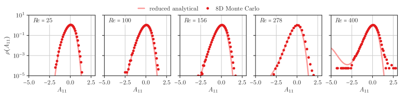
Figure 1: PDFs of the $A_{11}$ component of the velocity gradient tensor $A_{ij}=\partial u_{i}/\partial x_{j}$, for a range of Reynolds numbers. The red dots show a histogram of a DNS for the full RFD model (5), compared against the analytical prediction of the reduced RFD system (16) (solid line). It shows the emergence of another fixed point of the 1D reduced system at $A_{11}=-3.01$ for $R\mspace{-2.0mu}e=400$, which is an artifact of the model reduction.

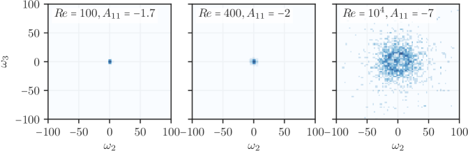
Figure 2: The joint PDF $\rho(\omega_{2},\omega_{3})$ of the perpendicular components of the vorticity, conditioned on relatively large negative strain values $A_{11}$, for different values of $R\mspace{-2.0mu}e$. As $R\mspace{-2.0mu}e$ increases, the originally very small variances around the most likely configuration $(\omega_{2},\omega_{3})=(0,0)$ grows in variance. At high $R\mspace{-2.0mu}e$, a zero perpendicular vorticity is no longer predominant. Instead, the most likely vorticity clusters on a ring, indicating a spontaneous symmetry breaking of the vorticity conditioned on large negative strain.

Here we give evidence for the validity of the dimensionally reduced model (16) for moderate $R\mspace{-2.0mu}e$, and the eventual symmetry breaking of the full 8D model (5). We recall that for the reduced RFD, an analytical PDF can be easily found by solving the corresponding Fokker-Planck equation Grigorio et al. (2017). Shown in figure 1 are the PDFs obtained via Monte Carlo (MC) simulations (red dots), in the range $R\mspace{-2.0mu}e\in[25,400]$, against the analytical PDFs of the reduced model (solid red lines). For the lowest $R\mspace{-2.0mu}e$ values up to $R\mspace{-2.0mu}e=156$, there is a reasonable agreement between the full 8D-RFD and the reduced 1D-RFD. For higher $R\mspace{-2.0mu}e$, a disagreement is seen in the right tail; note, though, that positive strain values are irrelevant for the development of large velocity gradients, as will be shown later. As $R\mspace{-2.0mu}e$ is increased further to $R\mspace{-2.0mu}e=400$ ($\tau/T=0.05$), at the very right of figure 1, the disagreement becomes more pronounced, including on the far left tail. Here, the 1D-RFD predicts a bimodal PDF with a new local minimum located at $A_{11}=-3.01$. By contrast, this bimodality is not observed in the 8D-RFD. The emergence of this bimodal profile remains for larger values of Reynolds number. Roughly $R\mspace{-2.0mu}e=400$ establishes the upper limit where the dimensional reduction can sensibly be applied.

The discrepancy between 8D-RFD and 1D-RFD demonstrates that for $R\mspace{-2.0mu}e\gtrsim 400$ the hypothesis of symmetries (axial and reflection) outlined in the previous section do not hold. As a consequence, other components of the velocity gradient start to play a role in the dynamics and may not be neglected. However, it remains true that the equation itself, and thus also the PDF, remains invariant under rotations and reflections for any value of the parameter $R\mspace{-2.0mu}e$. It is only individual sample trajectories that break the symmetry, while the statistics remain symmetric. Hence, it makes sense to borrow a terminology of condensed matter/high-energy physics, observing that the model undergoes spontaneous symmetry breaking, since the symmetry of the model is not realized by the individual states of the system $\mathbb{A}$, even though the PDF does observe it. The fact that this indeed happens can be shown numerically. Figure 2 shows the joint PDFs $\rho(\omega_{2},\omega_{3})$ of the perpendicular components of the vorticity $\omega_{i}=\epsilon_{ijk}\Omega_{kj}$, conditioned on relatively large negative $A_{11}$ at different $R\mspace{-2.0mu}e$. In other words, this shows the distribution of the vorticity vector in the presence of extreme strain, in the plane perpendicular to the strain axis. For moderate $R\mspace{-2.0mu}e=100$ and $400$ the distribution is concentrated around $0$, highlighting that the vorticity vector points along the strain axis (or is altogether zero). For very large $R\mspace{-2.0mu}e$, though, the perpendicular vorticity components prefer to occupy a ring away from $(0,0)$, indicating the breakdown of axisymmetry for the individual sample. At this $R\mspace{-2.0mu}e$, vorticity is more likely to be at an angle against the strain axis. Note that while we do not believe that the RFD model remains a valid description of 3D NSE turbulence in this regime, we remark that symmetry breaking has recently been observed for extreme strain events in full 3D Navier-Stokes Schorlepp et al. (2021).

It is worth mentioning that in same range of $R\mspace{-2.0mu}e$ where the symmetry breaking happens, the RFD model itself becomes problematic as well, as numerical instabilities start to appear, as reported by Chevillard and Meneveau (2006). Here, we shall briefly explain that by considering the high-$R\mspace{-2.0mu}e$ limit of (5). In the limit of infinite $R\mspace{-2.0mu}e$, the RFD model reduces to

$$\frac{d\mathbb{A}}{dt}=-\mathbb{A}^{2}+\frac{\text{Tr}(\mathbb{A}^{2})}{3}-\mathbb{A}+\sqrt{\varepsilon}\,\mathbb{W}\,.$$ (18)

Apart from the stochastic forcing, this equation corresponds to the linear damping closure proposed by Martín et al. (1998). It has been shown that the linear damping is not enough to counteract the strong non-linearities of the self-stretching and pressure Hessian terms, being subject to finite time singularities.

III.3 Dimensional reduction of the passive scalar RFD model

Following the same logic, one may derive a 2-dimensional reduced model for the PS-RFD by considering the statistics of only a single component of the passive scalar gradient, say $\psi_{1}=\nabla_{1}\theta$. More specifically, assuming now that both $\mathbb{A}$ and $\psi$ are invariant under rotation around the $x_{1}$ axis, the components $\psi_{2}$ and $\psi_{3}$ must vanish. As a result, the reduced version of the PS-RFD model (10) is defined as Grigorio (2020),

$$\frac{d\psi_{1}}{dt}=b(\psi_{1},a)+\sqrt{\varepsilon}\,\xi,$$ (19)

where

$$b(\psi_{1},a)=-\psi_{1}\,a-(e^{-\frac{2a}{\sqrt{R\mspace{-2.0mu}e}}}+2\,e^{\frac{a}{\sqrt{R\mspace{-2.0mu}e}}})\frac{\psi_{1}}{3\,T_{\theta}}\,,$$ (20)

and $\xi(t)$ is a white scalar noise that is independent of $\eta(t)$ in (16). The dynamics of $\psi_{1}(t)$ depend on the longitudinal velocity gradient $a(t)$. Thus, equation (19) has to be solved together with (16).

Being dependent on the RFD, it is clear that the dimensional reductions for PS-RFD will fail in the same range of $R\mspace{-2.0mu}e$ where RFD symmetry breaks down, but is in excellent agreement for $R\mspace{-2.0mu}e\lesssim 400$.

IV Instanton formalism and extreme events

In this section, we apply the instanton formalism to the PS-RFD model described in section II. Intuitively, the instanton formalism relies on the fact that in some limit (such as the small noise or extreme event limits) probabilities can be efficiently estimated through a prototypical “placeholder” event that observes the same scaling as the actual probability. A probability of an event is always a sum (or integral) over all possible ways the event can occur, weighted by its respective probability. In the limit, this integral can be approximated by a saddlepoint approximation or Laplace method, giving the leading order exponential contribution. For example, we are interested in the probability of observing events of extreme passive scalar gradients at final time, $P(\psi_{1}(t_{f})>z)$. Then, the instanton formalism postulates that the probability scales like an exponential,

$$P(\psi_{1}(t_{f})>z)\sim\exp\left(-\varepsilon^{-1}I(z)\right)\,.$$ (21)

The exponential scaling, given by the rate function $I(z)$, can be obtained by evaluating an action $S[\mathbb{A},\psi]$ at the instanton $(\mathbb{A}^{*},\psi^{*})$,

$$I(z)=S[\mathbb{A}^{*},\psi^{*}]=\inf_{\psi_{1}(t_{f})>z}S[\mathbb{A},\psi]\,,$$ (22)

where the instanton is the minimizer of the action. We will derive the action for the PS-RFD model in section IV.2. In our setup, the instanton formalism is equivalent to sample path large deviation theory Varadhan (1966); Dembo and Zeitouni (2010); Freidlin and Wentzell (2012).

IV.1 Related works

The action functional for the RFD model has first been determined in Moriconi et al. (2014). The instanton equations were linearized in this reference to derive an approximate analytical solution, with additional consideration of the fluctuations around the linearized instanton. As a result, to leading order in the perturbative expansion, the fluctuations yield an effective action with renormalized noise. That is, to first order, the fluctuations around the instanton can be taken into account by renormalizing the noise correlator. This approach was used to evaluate the PDFs of the velocity gradient and the joint PDF of the $R$ and $Q$ invariants.

By contrast, Grigorio et al. (2017) determines the instanton numerically by solving the corresponding highly non-linear RFD Hamilton’s equations with the Chernykh-Stepanov algorithm Chernykh and Stepanov (2001). Further, following the perturbation techniques outlined in Moriconi et al. (2014), a detailed analytical treatment of the RFD closure has been given by Apolinário et al. (2019), providing a hierarchical classification of several Feynman diagrams. In addition to the noise renormalization, Apolinário et al. (2019) also computes the propagator renormalization derived from linear instanton approximation. The resulting PDFs are compared with the ones from Grigorio et al. (2017) with good agreement.

More recently, Grigorio (2020) applies instanton arguments also to the PS-RFD model, proposing a parametric form of the Hamilton’s equation. Aside from that, a perturbation expansion has been carried out along the lines of Moriconi et al. (2014); Apolinário et al. (2019) to account for instanton path fluctuations.

Putting these results into perspective, all are capable of obtaining only mild non-Gaussian PDFs, that is, they work for a restricted range of $\tau$, namely, $\tau/T\geq 0.1$ ($R\mspace{-2.0mu}e\lesssim 100$). As $R\mspace{-2.0mu}e$ increases, and intermittency starts to play a role, the probability distributions develop heavy tails. Consequently, the corresponding rate function ceases to be convex, which prevents naive instanton approaches based on the Gärtner-Ellis theorem to remain well-posed. To overcome this, and apply the instanton formalism to more turbulent flows, here we introduce a nonlinear convexification to treat the heavy-tailed distribution, as discussed in section V.

IV.2 The action and instanton equations for the PS-RFD dynamics

In accordance with Grigorio (2020), the PS-RFD action reads Martin et al. (1973); Janssen (1976); de Dominicis (1976) ,

$$S[\mathbb{P},\mathbb{A},\Pi,\psi]=\int_{t_{i}}^{t_{f}}\text{d}t\, \left[\text{Tr}\left(\mathbb{P}^{\text{T}}(\dot{\mathbb{A}}-\mathbb{V}(\mathbb{A}))\right)-\frac{1}{2}P_{ij}G_{ijkl}P_{kl}\right.$$

$$\left.+\Pi^{\text{T}}(\dot{\psi}-M(\psi,\mathbb{A}))-\frac{1}{2}\Pi^{\text{T}}\Pi\right]\,,$$ (23)

where

$$M(\psi,\mathbb{A})=-\mathbb{A}^{\text{T}}\psi-\frac{\text{Tr}(\mathbb{C}^{-1})}{3T_{\theta}}\psi\,,$$ (24)

and

$$\mathbb{V}(\mathbb{A})=-\mathbb{A}^{2}+\frac{\mathbb{C}^{-1}\text{Tr}(\mathbb{A}^{2})}{\text{Tr}(\mathbb{C}^{-1})}-\frac{\text{Tr}(\mathbb{C}^{-1})}{3}\mathbb{A}\,,$$ (25)

stand for the drift terms of equations (10) and (5), respectively, and $\Pi\in\mathds{R}^{3}$ ($\mathbb{P}\in\mathds{R}^{3\times 3}$) is the conjugated momentum of $\psi$ ($\mathbb{A}$), closely related to the auxiliary variables of the Martin-Siggia-Rose-Janssen-de Dominicis formalism Martin et al. (1973); Janssen (1976); de Dominicis (1976).

The minimum of the action functional (IV.2) is achieved by the solutions of the following corresponding instanton equations of the fields $\mathbb{A},\psi$:

$$\begin{split}\frac{\delta S}{\delta P_{ij}}&=0,\ \Rightarrow\ \dot{A}_{ij}=V\left(\mathbb{A}\right)_{ij}+G_{ijkl}\,P_{kl},\\ \frac{\delta S}{\delta A_{ij}}&=0,\ \Rightarrow\ \dot{P}_{ij}=-P_{kl}\,\,\nabla_{A_{ij}}V\left(\mathbb{A}\right)_{kl}-\Pi_{k}\,\,\nabla_{A_{ij}}M\left(\psi,\mathbb{A}\right)_{k},\\ \frac{\delta S}{\delta\Pi_{k}}&=0,\ \Rightarrow\ \dot{\psi}_{k}=M\left(\psi,\mathbb{A}\right)_{k}+\Pi_{k},\\ \frac{\delta S}{\delta\psi_{k}}&=0,\ \Rightarrow\ \dot{\Pi}_{k}=-\Pi_{n}\,\,\nabla_{\psi_{k}}M\left(\psi,\mathbb{A}\right)_{n}\,,\end{split}$$ (26)

for $t\in[t_{i},t_{f}]$. The full formulas for these gradients are derived in appendix .2, where we expand the drifts up to second order Moriconi et al. (2014).

These four coupled equations (26) are solved simultaneously using the Chernykh-Stepanov (C-S) scheme Chernykh and Stepanov (2001); Grafke et al. (2013), which corresponds effectively to a gradient descent of the constrained optimization problem Grafke and Vanden-Eijnden (2019). The boundary conditions of (26) are specified by the choice of observable. Here, we are looking for events where one component $\psi_{j}$ of the passive scalar gradient exceeds a threshold $z$, which leads to

$$\mathbb{A}\left(t_{i}\right)=\textbf{0},\ \ \psi\left(t_{i}\right)=0,\ \ \mathbb{P}\left(t_{f}\right)=\textbf{0},\ \ \Pi_{j}\left(t_{f}\right)=\lambda\,\nabla F\left(\psi_{j}\left(t_{f}\right)\right),$$ (27)

where the initial values of the fields are their stable equilibrium points, the origin. The final time constraint on the gradient of passive scalar to attain $z=\psi_{j}\left(t_{f}\right)$ is implemented in (27) through a Lagrange multiplier $\lambda\in\mathds{R}$, Rindler (2018). The function $F:\mathds{R}\to\mathds{R}$ is a nonlinear reparametrization to ensure there is a unique $\lambda$ for every large passive scalar gradients of interest Alqahtani and Grafke (2021).

IV.3 Instantons for the reduced PS-RFD dynamics

The full instanton equations (26) correspond to the system (5), (10). However, when a final time constraint is imposed on a component of the passive scalar, such as $F\left(\psi_{1}\left(t_{f}\right)\right)$ (27), it exhibits symmetric behavior (with respect to axial and reflective symmetries) that reduce this 11-variables system to one with only two leading variables, $\psi_{1}\left(t\right)$ and $a\left(t\right)$. The same reduction applies to conditioning on other components of $\psi$. As discussed in section III, this reduction is valid for ${R\mspace{-2.0mu}e\lesssim 400}$.

For the reduced model (16), (19), the resulting 2D instanton equations are

$$\begin{split}&\dot{a}=v\left(a\right)+\,p,\\ &\dot{p}=-p\,\,\frac{\partial v\left(a\right)}{\partial a}-q\,\,\frac{\partial b\left(\psi_{1},a\right)}{\partial a},\\ &\dot{\psi}_{1}=b\left(\psi_{1},a\right)+q,\\ &\dot{q}=-q\,\,\ \frac{\partial b\left(\psi_{1},a\right)}{\partial\psi_{1}},\end{split}$$ (28)

where $p\left(t\right)=P_{11}\left(t\right)$ and $q\left(t\right)=\Pi_{1}\left(t\right)$. The drifts $v\left(a\right)$ and $b\left(\psi_{1},a\right)$ are derived in the reduced models’ section,  III, namely equations (17, 20).

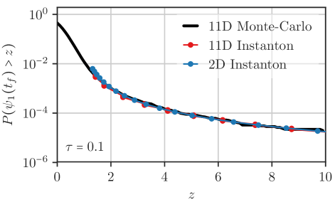
Figure 3: The complementary cumulative distribution functions of passive scalar gradients $P(\psi_{1}(t_{f})>z)$, (solid line) compared to the outcomes of both 11D and 2D instantons results (red and blue, respectively), with $R\mspace{-2.0mu}e=100$ and $T_{\theta}=1$. Both the full and the reduced instantons agree with MC simulations of the full system.

The difference between equations (26) and (28) is that the latter is more computationally efficient than the former due to the significant reduction of its dimensions, and we will use it in the following to estimate the tail probabilities of the passive scalar gradient. Figure 3 demonstrates numerically that this simplification is indeed justified for the instanton, as the predicted probabilities $P(\psi_{1}(t_{f})>z)$ of exceeding a passive scalar gradient $z$ at final time $t_{f}$ is in excellent agreement between MC sampling of the full RFD model, and the instanton estimates of both the full and the reduced models.

V Extreme gradient of the passive scalar

In this section we provide both analytical and numerical results for extreme passive scalar gradients in the PS-RFD. Starting from the model equations (7) and (10), which we rewrite here for convenience,

$$\frac{d\psi}{dt}=-\mathbb{A}^{\text{T}}\,\psi-\frac{\text{Tr}(\mathbb{C}^{-1})}{3T_{\theta}}\psi+\sqrt{\varepsilon}\,F\,;\quad\mathbb{C}=e^{\frac{\mathbb{A}}{\sqrt{R\mspace{-2.0mu}e}}}e^{\frac{\mathbb{A}^{\text{T}}}{\sqrt{R\mspace{-2.0mu}e}}}\,,$$ (29)

recall that the first term on the right hand side of this stochastic equation accounts for the advection, whereas the second term describes the effect of diffusion. We shall discuss the role played by parameters $T_{\theta}$ and $R\mspace{-2.0mu}e$. In the limit of high $R\mspace{-2.0mu}e$, the Cauchy-Green tensor $\mathbb{C}$ can be expanded to order $\mathcal{O}(R\mspace{-2.0mu}e^{-1})$,

$$\text{Tr}(\mathbb{C}^{-1}) =3+\frac{1}{2R\mspace{-2.0mu}e}\text{Tr}\left(\mathbb{A}^{2}+\mathbb{A}^{2\text{T}}+2\mathbb{A}^{\text{T}}\mathbb{A}\right)\,$$

$$=3+\frac{2}{R\mspace{-2.0mu}e}\text{Tr}\left(S^{2}\right)\,,$$ (30)

where, $S=(\mathbb{A}+\mathbb{A}^{\text{T}})/2$. Taking this into consideration equation (29) is rewritten as

$$\frac{d\psi}{dt}=-\mathbb{A}^{\text{T}}\,\psi-\frac{\psi}{T_{\theta}}-\frac{2\psi}{3T_{\theta}\,R\mspace{-2.0mu}e}\text{Tr}(S^{2})+\sqrt{\varepsilon}\,F\,.$$ (31)

From (31), it is clear that the second term on the right side is a linear damping for $\psi$, acting to decrease the size of fluctuations, with $T_{\theta}$ being the (dimensionless) characteristic time. The behavior of the third term, on the other hand, can be understood as follows: To leading order $\mathcal{O}(R\mspace{-2.0mu}e^{0})$, the variance of $\text{Tr}(S^{2})$ for the RFD depends on $\varepsilon$, with subleading correction of order $\mathcal{O}(R\mspace{-2.0mu}e^{-1})$ (Grigorio et al., 2017). Hence, we expect that as $R\mspace{-2.0mu}e$ increases while $T_{\theta}$ remains constant, the effect of the third term decreases on average.

Our claim is that, as $T_{\theta}$ or $R\mspace{-2.0mu}e$ is increased the damping effects are lowered in comparison to the advection term, which dominates the dynamics of the passive scalar gradient $\psi$. In turn, due to the minus sign accompanying the advection term, this transport term will drive an increase of a given component of $\psi$ as long as the eigenvalue of $\mathbb{A}$ along the same direction is negative, allowing for a growth of $\psi$ to extreme values.

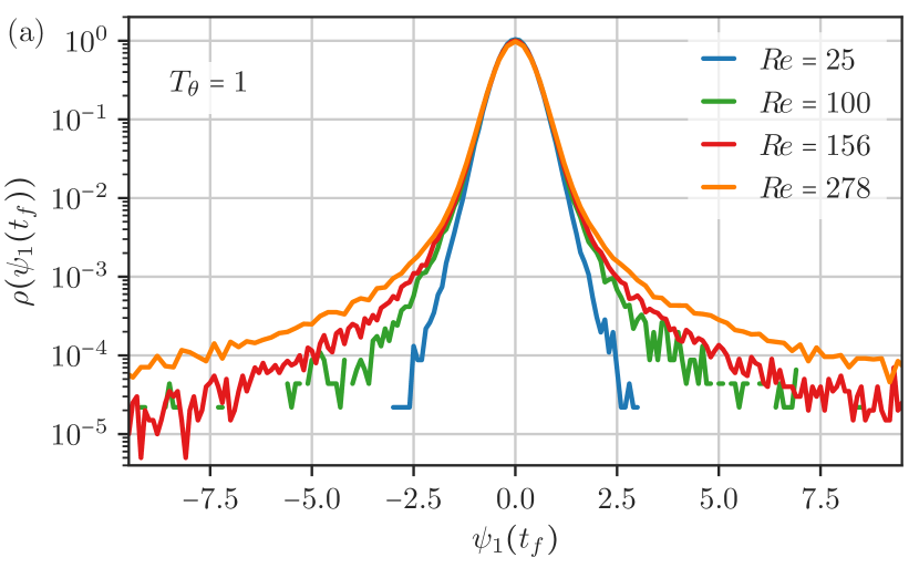
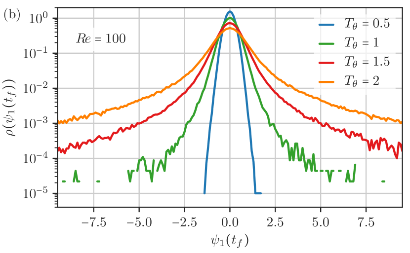
Figure 4: PDFs of the first component of passive scalar gradients, $\psi_{1}$, obtained from MC simulations of the PS-RFD system (5), (10) for various Reynolds numbers $R\mspace{-2.0mu}e$ and diffusive time scales $T_{\theta}$. Subfigure (a) exhibits heavier tails as $R\mspace{-2.0mu}e$ increases, where $T_{\theta}$ is set to unity, indicating significant turbulent mixing. Subfigure (b) shows that increasing $T_{\theta}$ at a moderate value of Reynolds number, $R\mspace{-2.0mu}e=100$, results in heavy-tailed gradient distributions, caused by a high transport rate.

V.1 High Reynolds number regime: Heavy tails and convexification

We are now equipped to investigate the probability to observe extreme passive scalar gradients for different $R\mspace{-2.0mu}e$ and $T_{\theta}$. Figure 4 displays the PDFs of the first component of passive scalar gradients, $\psi_{1}$, at the final time $t_{f}$, for various values of $R\mspace{-2.0mu}e$ in (a), and diffusive timescales $T_{\theta}$ in (b). They are obtained by MC simulations of the full 11D PS-RFD system (5,  10). It illustrates that indeed increasing both $R\mspace{-2.0mu}e$ and $T_{\theta}$ invokes heavy tails for the passive scalar gradient, due to strong turbulent mixing and high transport rates. We also remark that the fattening of the tails is more sensitive to the diffusive time scale $T_{\theta}$ than to the Reynolds number. This can be understood through equation (31), where it is evident that increasing $T_{\theta}$ leads to a decrease of two suppression terms for $\psi$, compared to only one for $R\mspace{-2.0mu}e$.

V.2 Extreme configurations of the passive scalar gradient

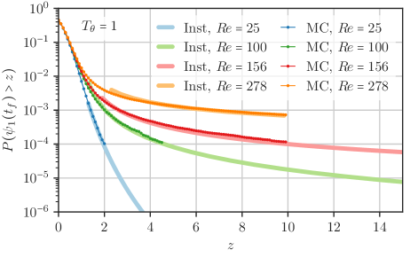
Figure 5: The complementary cumulative distribution functions of the passive scalar, $P(\psi_{1}(t_{f})>z)$. Compared are MC simulations (dotted lines) against 2D instantons estimates (solid lines) for different values of $R\mspace{-2.0mu}e$ ($T_{\theta}$ is set to unity). There is clear agreement between 11D MC and the 2D instanton estimate in particular when $\psi_{1}$ becomes large (far tails), in accordance with large deviations theory.

The probabilities obtained from MC sampling can be directly compared to predictions from the instanton formalism, obtained by solving the optimization problem (22). In practice, we do so by numerically solving the instanton equations (28). This comes of a significant performance benefit over computing the instanton for the full model (26), allowing us to compute the minimizer faster. For example the average speed-up factor for $R\mspace{-2.0mu}e=100$ and $z\in[2,10]$ is $54$. The benefit of solving equations (28) is even more significant for extreme events since this factor of improvement grows as $R\mspace{-2.0mu}e$ and/or $z$ increase. To overcome the problem of heavy tails, we convexify the rate function with a reparametrization of the observable according to the scheme presented in Alqahtani and Grafke (2021). Concretely, we choose ${F(z)=\mathrm{sign}(z)\log\log|z|}$, to be inserted as boundary condition into (27). We then use the C-S algorithm Chernykh and Stepanov (2001); Grafke et al. (2013) to obtain the instanton fields $\mathbb{A}$ and $\psi$ and its respective conjugate momenta $\mathbb{P}$ and $\Pi$. These allow us to (i) obtain the tail scaling of the passive scalar gradient PDF, by computing the action of the instanton, and (ii) identify the mechanism responsible for the formation of extreme passive scalar gradient events within the model.

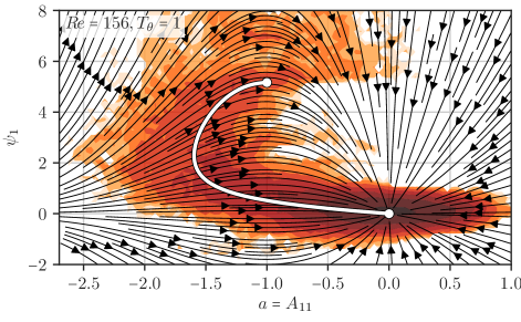
Figure 6: Events of extreme passive scalar gradient for the reduced model in the $a$-$\psi_{1}$-plane. The streamlines depict the deterministic drift of the reduced PS-RFD model. The line shows the instanton for realizing a final-time event of $\psi(t_{f})=5.16$, starting from the fixed point $(0,0)$ (white line). The density of trajectories of MC-simulations, conditioned on the same outcome, is shown as heatmap. Extreme outcomes of $\psi_{1}$ are commonly achieved by first transitioning into a region of negative strain, in which it is much easier to excite strong gradients. The instanton correctly predicts this mechanism.

Figure 5 presents the logarithmic probabilities of MC simulations of the passive scalar $\psi_{1}(t_{f})$ (dotted lines) against 2D instantons results (solid lines) for different values of $R\mspace{-2.0mu}e$, where $T_{\theta}$ is set to unity. It demonstrates an excellent agreement of the tail scaling between the 11D MC simulation and the instanton prediction, in particular when $\psi_{1}$ becomes large. Note that the instanton computation allows us to go extremely far into the tails, where MC becomes inefficient. Figure 6 depicts a set of realizations achieving an extreme passive scalar gradient, $\psi_{1}=5.16$, in the $a$-$\psi_{1}$ plane. Here, the shading indicates the density of trajectories that exhibit this large passive scalar gradient at the final time, while the solid line shows the instanton prediction for comparison. Clearly visible is the dominant mechanism for producing large passive scalar gradients: Fluctuations in the relevant strain component drives the system into a region of large negative strain, which deterministically amplifies the passive scalar gradient to large values. Note that the dominant reactive channel is nicely predicted by the instanton.

VI Conclusion

We investigate events of extreme passive scalar gradients in turbulent flows by using Lagrangian turbulence models extended to handle passive scalar advection. We demonstrate how a reduced two-dimensional model (one component of strain and passive scalar gradient each) captures the important mechanisms responsible for large passive scalar gradients. Notably, the symmetries necessary to apply the reduced model become broken for very extreme events or very large Reynolds numbers, which we can observe by direct sampling. We remark that the full RFD model also fails to describe fully developed Navier-Stokes turbulence in this regime, so that the reduced model remains a helpful simplification for our purposes.

We employ the instanton formalism to capture the scaling of very large outlier events in the tails of the PDF of passive scalar gradients. This most likely trajectory not only yields the correct tail scaling, even in the fat-tailed regime, but further allows us to investigate the mechanism responsible for the buildup of large gradients in the reduced model.

VII Appendix

.1 Statistical modeling of the fluid velocity gradient

The hypotheses that has been used to model both of the NSE and PSE, producing the RFD closure is summarized here, as follows;

• First, in Lagrangian coordinates $x\left(X,t\right)$ where $X$ is the initial position, the velocity is a function of time and initial position, making it feasible to visualize its history. Therefore, the main hypothesis of the RFD is that, due to the uncertainty of the deformation history resulting of the stochastic nature of turbulent flows, the history of the velocity gradient tensor $\mathbb{A}(t)$ has been forgotten, thus $\mathbb{A}$ depends only on its recent configuration, hence the name. In other words, the velocity gradient processes have been considered as Markov processes at which the future is independent of the past, given the current value.

• Based on the preceding hypothesis, the second assumption is that the Lagrangian pressure Hessian $\partial^{2}p/\left(\partial X_{m}\partial X_{l}\right)$ is an isotropic tensor, i.e., equals $a\,\delta_{ml}$, for any scalar $a$. This constant $a$ is selected in this model to be one-third of its trace, that is,

  $$\frac{\partial^{2}p}{\partial X_{m}\partial X_{l}}\approx\frac{1}{3}\frac{\partial^{2}p}{\partial X_{q}\partial X_{q}}\delta_{ml}.$$

  As a result, using the chain rule and neglecting higher order terms, the pressure term of equation (3) is modeled as:

  $$\frac{\partial^{2}p}{\partial x_{i}\partial x_{j}}\approx\frac{\partial X_{m}}{\partial x_{i}}\frac{\partial X_{l}}{\partial x_{j}}\frac{\partial^{2}p}{\partial X_{m}\partial X_{l}}\approx\frac{\partial X_{m}}{\partial x_{i}}\frac{\partial X_{l}}{\partial x_{j}}\frac{1}{3}\frac{\partial^{2}p}{\partial X_{q}\partial X_{q}}\delta_{ml}=-\frac{\text{Tr}(\mathbb{A}^{2})}{\text{Tr}(\mathbb{C}^{-1})}\,C_{ij}^{-1},$$ (32)

  where the last equality comes from utilizing the Poisson equation to express $p$ in terms of $\mathbb{A}$ (i.e. by taking the divergence of the NSE (1) and employing the divergence free property). The tensor

  $${C_{ij}=\frac{\partial x_{i}}{\partial X_{m}}\,\frac{\partial x_{j}}{\partial X_{l}}\,\delta_{ml}\approx\exp\left(\tau\mathbb{A}\right)\exp\left(\tau\mathbb{A}^{\text{T}}\right)},$$ (33)

  is a stationary Cauchy-Green tensor, where $\tau$ is the decorrelation time scale after which any correlation of $\mathbb{A}$ is neglected, based on the main hypothesis given earlier. This parameter $\tau$ is proportional to $R\mspace{-2.0mu}e^{-1/2}$. It therefore plays an essential role of the dynamics of this model, more discussion is in section V.1.

• The Lagrangian viscous Hessian of $\mathbb{A}$ has been treated as a classical linear damping term, i.e., ${\nu\ \mathbb{A}/(\partial X_{m}\partial X_{l})\approx-\nu\ \mathbb{A}/(3T)}$ where a dimensional argument used to write $\nu/\left(\partial X\right)^{2}\sim T^{-1}$, and $T$ is considered to be on the order of the integral time scale of the flow. Finally, the model of the viscous term of (3) becomes:

  $$\nu\ \frac{\partial^{2}\mathbb{A}}{\partial x_{n}\partial x_{n}}\approx\nu\ \frac{\partial X_{m}}{\partial x_{n}}\frac{\partial X_{l}}{\partial x_{n}}\frac{\partial^{2}\mathbb{A}}{\partial X_{m}\partial X_{l}}\approx-\frac{\text{Tr}(\mathbb{C}^{-1})}{3T}\mathbb{A}.$$ (34)

  Notice that the diffusivity term of equation (8) is modeled using the same assumptions of the viscosity term, yielding to

  $$\kappa\ \frac{\partial^{2}\psi}{\partial x_{j}\partial x_{j}}\approx-\frac{\text{Tr}(\mathbb{C}^{-1})}{3T_{\theta}}\psi,\ \ \ \ \ \ \ \ \kappa/\left(\partial X_{\theta}\right)^{2}\sim T_{\theta}^{-1}\,,$$ (35)

where $\partial X_{\theta}$ is related to the smallest scales structures of the passive scalar. Finally, substituting the foregoing closed terms (32,34) into the Lagrangian velocity gradient equation (3) produces the velocity gradient RFD model (4). In the same manner, replacing the closed diffusive term (35) of the Lagrangian passive scalar gradient equation (8) yields the RFD model of the passive scalar (9).

.2 The detailed derivations of the gradients of the drifts

To compute the gradient of the exponential terms of $V\left(\mathbb{A}\right)$ and $M\left(\psi,\mathbb{A}\right)$ with respect tensor $\mathbb{A}$, it needs to be extended. Up to the second order of $\tau$, the power series of the matrix exponential $e^{\textbf{X}}=\sum_{n=0}^{\infty}\frac{\textbf{X}^{n}}{n!}$ is used for the stationary Cauchy-Green tensor $\mathbb{C}^{-1}$. Notice that it still possesses the physical features of the full drifts of this model Moriconi et al. (2014). The expansion process is ordered in the following points:

• The power series of the matrix exponential to extend $\mathbb{C}^{-1}$ gives:

  $$\mathbb{C}^{-1} =\left(e^{\tau\mathbb{A}}\,\,e^{\tau\mathbb{A}^{\text{T}}}\right)^{-1}$$

  $$=\left(\sum_{n=0}^{\infty}\frac{\left(-\tau\mathbb{A}^{\text{T}}\right)^{n}}{n!}\right)\left(\sum_{n=0}^{\infty}\frac{\left(-\tau\mathbb{A}\right)^{n}}{n!}\right)$$

  $$=\mathbb{I}-\tau\,(\mathbb{A}+\mathbb{A}^{\text{T}})+\frac{\tau^{2}}{2}\left(\mathbb{A}^{2}+2\,\mathbb{A}^{\text{T}}\mathbb{A}+\left(\mathbb{A}^{\text{T}}\right)^{2}\right)+O\left(\tau^{3}\right).$$

  Then, the trace of $\mathbb{C}^{-1}$ after the truncation to the second order is

  $$\text{Tr}\left(\mathbb{C}^{-1}\right)=3+\tau^{2}\,\text{Tr}\left(\mathbb{A}^{2}\right)+\tau^{2}\,\text{Tr}\left(\mathbb{A}^{\text{T}}\mathbb{A}\right),$$ (36)

  where the linearity property of the trace operator and the fact that $\text{Tr}\left(\mathbb{A}\right)=\text{Tr}\left(\mathbb{A}^{\text{T}}\right)=0$ (due to incompressibility) and $\text{Tr}\left(\mathbb{A}^{2}\right)=\text{Tr}\left(\left(\mathbb{A}^{\text{T}}\right)^{2}\right)$ are used.

• Substituting the expanded version of $\mathbb{C}^{-1}$ and its trace in the drift term (25) gives:

  $$\begin{split}V\left(\mathbb{A}\right)&=-\mathbb{A}^{2}+\frac{\text{Tr}(\mathbb{A}^{2})}{3+\tau^{2}\,\text{Tr}\left(\mathbb{A}^{2}\right)+\tau^{2}\,\text{Tr}\left(\mathbb{A}^{\text{T}}\mathbb{A}\right)}\,\,\biggl{[}\mathbb{I}-\tau\,\left(\mathbb{A}+\mathbb{A}^{\text{T}}\right)+\\ &\,\,\,\,\,\,\,\frac{\tau^{2}}{2}\biggl{(}\mathbb{A}^{2}+2\,\mathbb{A}^{\text{T}}\mathbb{A}+\left(\mathbb{A}^{\text{T}}\right)^{2}\biggr{)}\biggr{]}-\frac{\mathbb{A}}{3}\ \biggl{[}3+\tau^{2}\,\text{Tr}\left(\mathbb{A}^{2}\right)+\tau^{2}\,\text{Tr}\left(\mathbb{A}^{\text{T}}\mathbb{A}\right)\biggr{]}.\end{split}$$ (37)

  The quantity $1/(3+\tau^{2}\,\text{Tr}\left(\mathbb{A}^{2}\right)+\tau^{2}\,\text{Tr}\left(\mathbb{A}^{\text{T}}\mathbb{A}\right))$ can be rewritten in terms of Maclaurin series as follows,

  $$\frac{1}{3\left(1-x\right)}=\frac{1}{3}\sum_{n=0}^{\infty}x^{n},\ \ \ \ \ x\coloneqq-\frac{1}{3}\biggl{(}\tau^{2}\,\text{Tr}\left(\mathbb{A}^{2}\right)+\tau^{2}\,\text{Tr}\left(\mathbb{A}^{\text{T}}\mathbb{A}\right)\biggr{)}.$$

  Thus,

  $$\frac{1}{3+\tau^{2}\,\text{Tr}\left(\mathbb{A}^{2}\right)+\tau^{2}\,\text{Tr}\left(\mathbb{A}^{\text{T}}\mathbb{A}\right)}=\frac{1}{3}-\frac{1}{9}\biggl{(}\tau^{2}\,\text{Tr}\left(\mathbb{A}^{2}\right)+\tau^{2}\,\text{Tr}\left(\mathbb{A}^{\text{T}}\mathbb{A}\right)\biggr{)}+O\left(\tau^{3}\right).$$

• Inserting the last equality into equation (37) and considering only the second order terms of $\tau$ yields the truncation formula of $V\left(\mathbb{A}\right)$ (25), Grigorio et al. (2017):

  $$V\left(\mathbb{A}\right)=\sum_{p=1}^{4}V_{p}\left(\mathbb{A}\right),$$ (38)

  where $V_{p}\left(\mathbb{A}\right)$ contains all the components of $O\left(\mathbb{A}^{p}\right)$, that is:

  $$V_{1}\left(\mathbb{A}\right)=-\mathbb{A},$$

  $$V_{2}\left(\mathbb{A}\right)=-\mathbb{A}^{2}+\frac{\mathbb{I}}{3}\text{Tr}(\mathbb{A}^{2}),$$

  $$V_{3}\left(\mathbb{A}\right)=-\frac{\tau}{3}\,\text{Tr}(\mathbb{A}^{2})\left(\mathbb{A}+\mathbb{A}^{\text{T}}\right)-\frac{\tau^{2}}{3}\,\mathbb{A}\,\left(\,\text{Tr}\left(\mathbb{A}^{2}\right)+\,\text{Tr}\left(\mathbb{A}^{\text{T}}\mathbb{A}\right)\right),$$

  $$\begin{split}V_{4}\left(\mathbb{A}\right)&=-\frac{\tau^{2}}{9}\,\text{Tr}(\mathbb{A}^{2})\,\mathbb{I}\,\left(\text{Tr}(\mathbb{A}^{2})+\text{Tr}(\mathbb{A}^{\text{T}}\mathbb{A})\right)\\ &\,\,\,\,\,\,\,\,+\frac{\tau^{2}}{6}\,\text{Tr}(\mathbb{A}^{2})\left(\mathbb{A}^{2}+2\,\mathbb{A}^{\text{T}}\,\mathbb{A}+\left(\mathbb{A}^{\text{T}}\right)^{2}\right).\end{split}$$

• Similarly, the extension version of $M\left(\psi,\mathbb{A}\right)$, resulting from substituting the truncated trace (36) into the drift of the PS-RFD (24), is

  $$M\left(\psi,\mathbb{A}\right)=-\mathbb{A}^{\text{T}}\,\psi-\frac{1}{3\,T_{\theta}}\biggl{(}3+\tau^{2}\,\text{Tr}\left(\mathbb{A}^{2}\right)+\tau^{2}\,\text{Tr}\left(\mathbb{A}^{\text{T}}\mathbb{A}\right)\biggr{)}\,\,\psi.$$ (39)

Now, obtaining the gradient tensors $\nabla_{A_{ij}}V\left(\mathbb{A}\right)_{kl}$, $\ \nabla_{A_{ij}}M\left(\psi,\mathbb{A}\right)_{k}$ and $\ \nabla_{\psi_{k}}M\left(\psi,\mathbb{A}\right)_{n}$ (required for instanton equations (26) ) from the truncated drifts (38, 39) is straightforward computations, as shown:

• The first gradient tensor is

  $$\begin{split}\left(\nabla_{\mathbb{A}}V\left(\mathbb{A}\right)\right)_{klij}=\nabla_{A_{ij}}V\left(\mathbb{A}\right)_{kl}=\sum_{p=1}^{4}\nabla_{A_{ij}}V_{p}\left(\mathbb{A}\right)_{kl},\end{split}$$ (40)

  where,

  $$\nabla_{A_{ij}}V_{1}\left(\mathbb{A}\right)_{kl}=-\frac{\partial A_{kl}}{\partial A_{ij}}=-\delta_{ki}\delta_{lj},$$

  $$\nabla_{A_{ij}}V_{2}\left(\mathbb{A}\right)_{kl} =\frac{\partial}{\partial A_{ij}}\left[-A_{kl}^{2}+\frac{1}{3}\,\delta_{kl}\,\text{Tr}(\mathbb{A}^{2})\right]$$

  $$=-\delta_{ki}\,A_{jl}-A_{ki}\,\delta_{lj}+\frac{2}{3}\,\delta_{kl}\,A_{ji},$$

  $$\begin{split}\nabla_{A_{ij}}V_{3}\left(\mathbb{A}\right)_{kl}&=-\frac{\tau}{3}\frac{\partial}{\partial A_{ij}}\biggl{[}\text{Tr}(\mathbb{A}^{2})\left(A_{kl}+A_{lk}\right)+\tau\,A_{kl}\left(\text{Tr}(\mathbb{A}^{2})+\text{Tr}(\mathbb{A}^{\text{T}}\mathbb{A})\,\right)\biggr{]}\\ &=-\frac{\tau}{3}\left(2\,A_{ji}\left(A_{kl}+A_{lk}\right)+\text{Tr}(\mathbb{A}^{2})\,\left(\delta_{ki}\,\delta_{lj}+\delta_{li}\,\delta_{kj}\right)\right)\\ &-\frac{\tau^{2}}{3}\left(\delta_{ki}\,\delta_{lj}\left(\text{Tr}(\mathbb{A}^{2})+\text{Tr}(\mathbb{A}^{\text{T}}\mathbb{A})\,\right)+2A_{kl}\left(\,A_{ji}+\,A_{ij}\right)\right),\end{split}$$

  $$\begin{split}\nabla_{A_{ij}}V_{4}\left(\mathbb{A}\right)_{kl}=\frac{\partial}{\partial A_{ij}}\biggl{[}&-\frac{\tau^{2}}{9}\,\text{Tr}(\mathbb{A}^{2})\,\delta_{kl}\,\left(\text{Tr}(\mathbb{A}^{2})+\text{Tr}(\mathbb{A}^{\text{T}}\,\mathbb{A})\right)\\ &+\frac{\tau^{2}}{6}\,\text{Tr}(\mathbb{A}^{2})\,\left(A^{2}_{kl}+2\,A_{mk}\,A_{ml}+A^{2}_{lk}\right)\biggr{]}\\ &=-\frac{2}{9}\,\tau^{2}\,\delta_{kl}\,\biggl{[}A_{ji}\,\left(2\,\text{Tr}(\mathbb{A}^{2})+\text{Tr}(\mathbb{A}^{\text{T}}\mathbb{A})\,\right)+\text{Tr}(\mathbb{A}^{2})\,A_{ij}\biggr{]}\\ &+\frac{\tau^{2}}{3}\biggl{[}A_{ji}\,\left(A^{2}_{kl}+2A_{mk}\,A_{ml}\,+A^{2}_{lk}\right)+\text{Tr}(\mathbb{A}^{2})\,\biggl{(}\,\delta_{kj}\,A_{il}\,+A_{ik}\,\delta_{lj}\\ &+\frac{1}{2}\left(\delta_{ki}\,A_{jl}+A_{ki}\,\delta_{lj}+\delta_{li}\,A_{jk}+A_{li}\,\delta_{kj}\right)\biggr{)}\biggr{]}.\end{split}$$

  The following relations are used:

  $$\frac{\partial A^{2}_{kl}}{\partial A_{ij}}=\delta_{ki}\,A_{jl}+A_{ki}\,\delta_{lj},\ \ \ \ \frac{\partial\,\text{Tr}(\mathbb{A}^{2})}{\partial A_{ij}}=A_{ji}+A_{ji}=2A_{ji},\ \ \ \ \frac{\partial\,\text{Tr}(\mathbb{A}^{\text{T}}\mathbb{A})}{\partial A_{ij}}=2A_{ij}.$$

• The second gradient tensor is

  $$\begin{split}\left(\nabla_{\mathbb{A}}M\left(\psi,\mathbb{A}\right)\right)_{kij}=\nabla_{A_{ij}}M\left(\psi,\mathbb{A}\right)_{k}&=\frac{\partial}{\partial A_{ij}}\biggl{[}-A_{mk}\,\psi_{m}\\ &-\frac{1}{3\,T_{\theta}}\biggl{(}3+\tau^{2}\,\text{Tr}(\mathbb{A}^{2})+\tau^{2}\,\text{Tr}(\mathbb{A}^{\text{T}}\mathbb{A})\biggr{)}\,\,\psi_{k}\biggr{]}\\ &=-\delta_{kj}\psi_{i}-\frac{2\,\tau^{2}}{3\,T_{\theta}}\left(A_{ji}+A_{ij}\right)\,\,\psi_{k}.\end{split}$$ (41)

• The third gradient tensor is

  $$\begin{split}\left(\nabla_{\psi}M\left(\psi,\mathbb{A}\right)\right)_{nk}=\nabla_{\psi_{k}}M\left(\psi,\mathbb{A}\right)_{n}&=\frac{\partial}{\partial\psi_{k}}\left[-A_{mn}\,\psi_{m}-\frac{1}{3\,T_{\theta}}\biggl{(}3+\tau^{2}\,\text{Tr}(\mathbb{A}^{2})+\tau^{2}\,\text{Tr}(\mathbb{A}^{\text{T}}\mathbb{A})\biggr{)}\,\,\psi_{k}\right]\\ &=-A_{kn}-\frac{1}{3\,T_{\theta}}\biggl{(}3+\tau^{2}\,\text{Tr}(\mathbb{A}^{2})+\tau^{2}\,\text{Tr}(\mathbb{A}^{\text{T}}\mathbb{A})\biggr{)}\,\,\delta_{nk}.\end{split}$$ (42)

References

- Shraiman and Siggia (2000) B. I. Shraiman and E. D. Siggia, Nature 405, 639 (2000).
- Falkovich et al. (2001) G. Falkovich, K. Gawedzki, and M. Vergassola, Reviews of Modern Physics 73, 913 (2001).
- Frisch (1995) U. Frisch, Turbulence (Cambridge University Press, Cambridge, 1995).
- Vieillefosse (1982) P. Vieillefosse, Journal de Physique 43, 837 (1982).
- Vieillefosse (1984) P. Vieillefosse, Physica A: Statistical Mechanics and its Applications 125, 150 (1984).
- Cantwell (1992) B. J. Cantwell, Physics of Fluids A: Fluid Dynamics 4, 782 (1992).
- Meneveau (2011) C. Meneveau, Annual Review of Fluid Mechanics 43, 219 (2011).
- Wallace (2009) J. M. Wallace, Physics of Fluids 21, 021301 (2009).
- Girimaji and Pope (1990) S. S. Girimaji and S. B. Pope, Physics of Fluids A: Fluid Dynamics 2, 242 (1990).
- Chertkov et al. (1999) M. Chertkov, A. Pumir, and B. I. Shraiman, Physics of fluids 11, 2394 (1999).
- Chevillard and Meneveau (2006) L. Chevillard and C. Meneveau, Physical Review Letters 97, 174501 (2006).
- Jeong and Girimaji (2003) E. Jeong and S. S. Girimaji, Theoretical and Computational Fluid Dynamics 16, 421 (2003).
- Gonzalez (2009) M. Gonzalez, Physics of Fluids 21, 055104 (2009).
- Hater et al. (2011) T. Hater, H. Homann, and R. Grauer, Physical Review E 83, 017302 (2011).
- Grafke et al. (2015a) T. Grafke, R. Grauer, and S. Schindel, Communications in Computational Physics 18, 577 (2015a).
- Freidlin and Wentzell (2012) M. I. Freidlin and A. D. Wentzell, Random perturbations of dynamical systems, Vol. 260 (Springer, 2012).
- Balkovsky et al. (1997) E. Balkovsky, G. Falkovich, I. Kolokolov, and V. Lebedev, Physical Review Letters 78, 1452 (1997).
- Grafke et al. (2014) T. Grafke, R. Grauer, T. Schäfer, and E. Vanden-Eijnden, Multiscale Modeling & Simulation 12, 566 (2014).
- Grafke et al. (2015b) T. Grafke, R. Grauer, and T. Schäfer, Journal of Physics A: Mathematical and Theoretical 48, 333001 (2015b).
- Laurie and Bouchet (2015) J. Laurie and F. Bouchet, New Journal of Physics 17, 015009 (2015).
- Dematteis et al. (2019) G. Dematteis, T. Grafke, M. Onorato, and E. Vanden-Eijnden, Physical Review X 9, 041057 (2019).
- Tong et al. (2021) S. Tong, E. Vanden-Eijnden, and G. Stadler, arXiv:2007.13930 [math.OC] (2021).
- Alqahtani and Grafke (2021) M. Alqahtani and T. Grafke, Journal of Physics A: Mathematical and Theoretical 54, 175001 (2021).
- Grigorio et al. (2017) L. S. Grigorio, F. Bouchet, R. M. Pereira, and L. Chevillard, Journal of Physics A: Mathematical and Theoretical 50, 055501 (2017).
- Grigorio (2020) L. S. Grigorio, Journal of Physics A: Mathematical and Theoretical 53, 445001 (2020).
- Schorlepp et al. (2021) T. Schorlepp, T. Grafke, S. May, and R. Grauer, arXiv:2107.06153 [physics] (2021).
- Martín et al. (1998) J. Martín, C. Dopazo, and L. Valiño, Physics of Fluids 10, 2012 (1998).
- Varadhan (1966) S. R. S. Varadhan, Communications on Pure and Applied Mathematics 19, 261 (1966).
- Dembo and Zeitouni (2010) A. Dembo and O. Zeitouni, Large deviations techniques and applications (Springer-Verlag, Berlin, 2010).
- Moriconi et al. (2014) L. Moriconi, R. M. Pereira, and L. S. Grigorio, Journal of Statistical Mechanics: Theory and Experiment 2014, P10015 (2014).
- Chernykh and Stepanov (2001) A. I. Chernykh and M. G. Stepanov, Physical Review E 64, 026306 (2001).
- Apolinário et al. (2019) G. B. Apolinário, L. Moriconi, and R. M. Pereira, Physical Review E 99, 033104 (2019).
- Martin et al. (1973) P. C. Martin, E. D. Siggia, and H. A. Rose, Physical Review A 8, 423 (1973).
- Janssen (1976) H.-K. Janssen, Zeitschrift für Physik B Condensed Matter 23, 377 (1976).
- de Dominicis (1976) C. de Dominicis, J. Phys. C 1, 247 (1976).
- Grafke et al. (2013) T. Grafke, R. Grauer, and T. Schäfer, Journal of Physics A: Mathematical and Theoretical 46, 062002 (2013).
- Grafke and Vanden-Eijnden (2019) T. Grafke and E. Vanden-Eijnden, Chaos: An Interdisciplinary Journal of Nonlinear Science 29, 063118 (2019).
- Rindler (2018) F. Rindler, Calculus of Variations (Springer, 2018).