Which Bridges Are Weak Ties? Algebraic Topological Insights on Network Structure and Tie Strength

Abstract

Bridging relationships between individuals situated in different parts of a social network are important conduits for information and resources in social and organizational settings. Dyadic tie strength has often been used as an indicator for whether a relationship is bridging, under the assumption that bridging ties are always weak ties. However, recent empirical evidence suggests that bridging ties are often strong, forcing us to rethink the relationship between social network structure and dyadic tie strength. Here, we provide an analysis based on algebraic topology which clarifies this relationship between network structure and dyadic tie strength. Rather than model the network as a graph, we use a simplicial complex which can explicitly encode group interactions between three or more individuals. First, we show theoretically and empirically that Edge PageRank, an algebraic topological measure originally defined as an extension of the classical PageRank measure, is a valid continuous measure of how well a relationship acts as a bridge. Second, we use the tool of Hodge Decomposition, which allows us to decompose any flow in a simplicial complex into three orthogonal components, to clarify the relationship between dyadic tie strength and network structure. We find that individuals invest less in relationships associated with topological holes in the network, replicating and explaining recent empirical results that bridging relationships spanning short network distances tend to be weak, whereas those spanning longer distances are strong. Our results are validated on 15 large scale datasets and suggest the value of algebraic topological methods in empirical network analysis.

1 Introduction

For over five decades, researchers across the social sciences have focused on determining which social connections provide the most valuable information to an individual (Aral 2016, Burt 2002, Gilbert and Karahalios 2009, Granovetter 1973, Mattie et al. 2018, Park et al. 2018, Smith 2005). Having advantageous social connections has been shown at length to positively impact outcomes including job placement (Smith 2005, Granovetter 1973), promotion (Burt 2000), creativity (Uzzi and Spiro 2005), innovation (Burt 2002), political success (Padgett and Ansell 1993), productivity (Aral et al. 2007, Reagans and Zuckerman 2001), and knowledge transfer in organizations (Hansen 1999, Aral and Dhillon 2022). A core finding in this literature is that bridging relationships, i.e. social ties between individuals situated in different parts of the social network, are uniquely valuable. Bridging relationships allow one access to novel information (Granovetter 1973), position one to have control over network resources (Burt 2000), and can enable one to find distinct leadership opportunities (Jackson 2020). As such, identifying bridging ties in social and organizational networks is critical in being able to optimally mobilize one’s social network (Rajkumar et al. 2022).

One of the foundational arguments which emphasizes the importance of bridging ties comes from Granovetter (1973)’s “The Strength of Weak Ties.” Tie strength refers to an attribute of a particular dyadic relationship which at minimum encodes “the amount of time spent interacting with someone, the level of intimacy, the level of emotional intensity, and the level of reciprocity” between two individuals (Granovetter 1973). Granovetter argues that bridging ties should always be weak, via an assumption he refers to as the absence of the “Forbidden Triad.” This assumption states that if individuals $A$ and $B$ share a strong tie, and $A$ and $C$ share a strong tie, then there must be at least some tie (whether strong or weak) between $B$ and $C$. It can be shown that bridging ties under this assumption are necessarily weak, except under the unlikely condition where one of the individuals in the bridge has no strong ties. Hence, Granovetter provides a simple yet powerful intuition: whereas close family and friends (strong ties) may have similar sources of information to an individual, acquaintances (weak ties) may have access to different resources altogether which could potentially expand the social reach of an agent.

However, recent evidence has shown that the relationship between the dyadic notion of tie strength and whether a relationship is bridging is more complex than Granovetter (1973)’s original argument suggests. When tie strength is viewed as a continuum, data from population-scale networks has shown that there is a “U”-shaped relationship between the tie strength of a dyad and the range of a tie, where range refers to the length of the second-shortest path between two nodes in a network (Park et al. 2018). That is, the ties which span the longest network distance are surprisingly strong, contradicting Granovetter’s original argument.

In this work, we use algebraic topology to clarify this complex relationship between bridging relationships and the dyadic notion of tie strength. First, we show that the Edge PageRank measure recently introduced by Schaub et al. (2020) can be interpreted as a valid measure of the extent to which a relationship is bridging or not. Specifically, whereas the measure was previously introduced as an algebraic topological extension of the standard PageRank measure for nodes, here we show that the stochastic process which underlies the Edge PageRank measure can be interpreted as an information exchange process which emphasizes ties that are well-positioned to be conduits for novel information. This allows us to treat Edge PageRank as a continuous measure of the extent to which a social tie acts as a bridge between communities, as opposed to previous combinatorial definitions. Second, we apply the tool of Hodge Decomposition to intuitively extend Granovetter (1973)’s “Forbidden Triad,” suggesting a novel theory relating social network structure do the dyadic notion of tie strength. For both sets of results, we provide evidence for our conclusions with experiments across fifteen large scale social network datasets.

The Algebraic Topological Approach

The core difference between the algebraic topological approach taken here and previous work is that we encode higher order interactions between three or more individuals into our analysis. Previous work relies on representing the interactions in the social network with a set of dyadic edges, such that only relationships between pairs of individuals can be modeled. However, social interactions often take place among groups larger than two, inherently limiting existing approaches, and much of the information collected on social networks goes beyond dyads (Benson et al. 2018). We incorporate the information from higher order interactions by modeling network information with a more general mathematical structure called a simplicial complex, as opposed to a graph. This allows us to explicitly distinguish between a group interaction among three people, and the case where only pairwise interactions exist. For simplicity, we assume that we have a dataset of interactions where each interaction is between two or three nodes (people in the social network). We call the interactions involving two nodes edges and those among three nodes triangles. For notation, we will assume we have $n$ nodes, $e$ edges, and $t$ triangles in the dataset.

Such a rich data representation allows us to use a larger set of tools and centrality measures, including the recently-developed Edge PageRank measure (Schaub et al. 2020). The Edge PageRank measure was developed as a mathematical extension of the node PageRank measure commonly used in network analysis (Page et al. 1999). Specifically, the node PageRank measure can be written as a function of the normalized graph Laplacian matrix denoted by $\mathcal{L}_{0}\in\mathbb{R}^{n\times n}$, and Schaub et al. (2020) showed that there exists a normalization for the graph Laplacian which operates on edges, which they refer to as a normalized Hodge Laplacian $\mathcal{L}_{1}\in\mathbb{R}^{e\times e}$. The normalized Hodge Laplacian can be used to define a personalized Edge PageRank vector for each edge in the simplicial complex, and the $2$-norm of this vector is referred to as the Edge PageRank score of an edge.

Here, we show that the Edge PageRank measure can be viewed as the outcome of a natural social process, similar to node PageRank and Katz centrality (Page et al. 1999, Katz 1953, Friedkin and Johnsen 1990). More specifically, we define a random, local interaction process, where each state is a directed communication from one node to another along an edge, and the possible transitions between states are dictated by the presence of both edges and triangles in the network. After the random process reaches a steady state, such that each possible directed communication is assigned a probability, the measure then takes a difference between the two probabilities corresponding to orientations of each edge. In this way, an edge receives a large value if there is asymmetric communication in the steady state of the random process, indicating that there is low communication bandwidth in one direction and suggesting the tie is weak (Aral and Van Alstyne 2011, Reagans and Zuckerman 2001). Based on how the presence of triangles affects the random process, the net result appropriately discounts the effect of triadic interactions, allowing the measure to reflect when an edge spans a topological hole in a network (Figure 1(c)). This discounting effect is consistent with the commonly accepted idea that information shared in triads likely to have redundancies, c.f. Aral and Van Alstyne (2011).

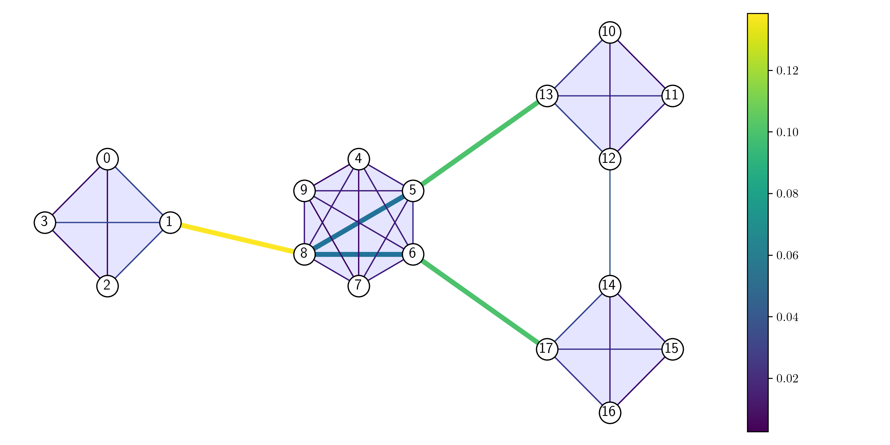
(a) Betweenness Centrality

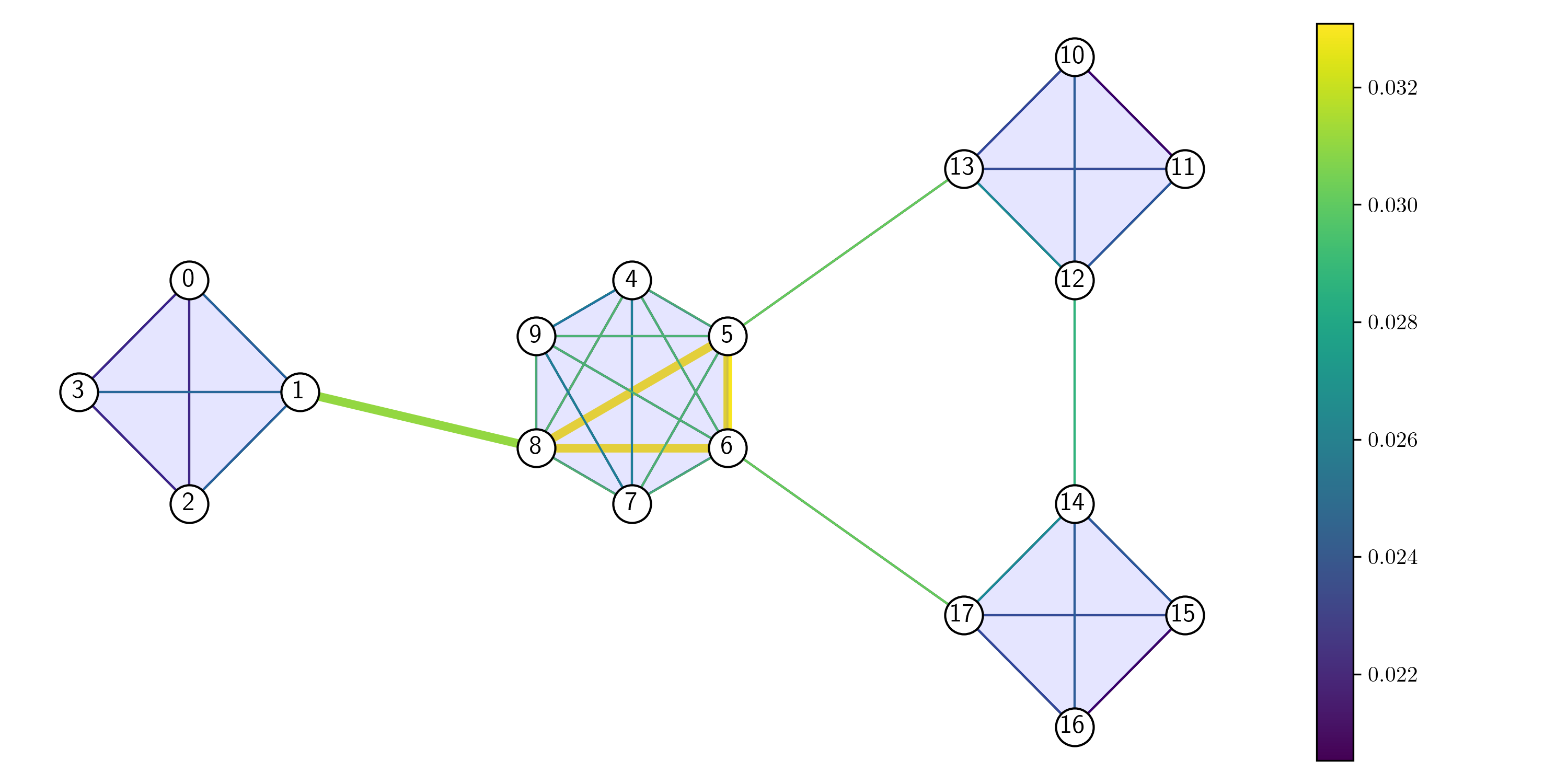
(b) PageRank on the Line Graph

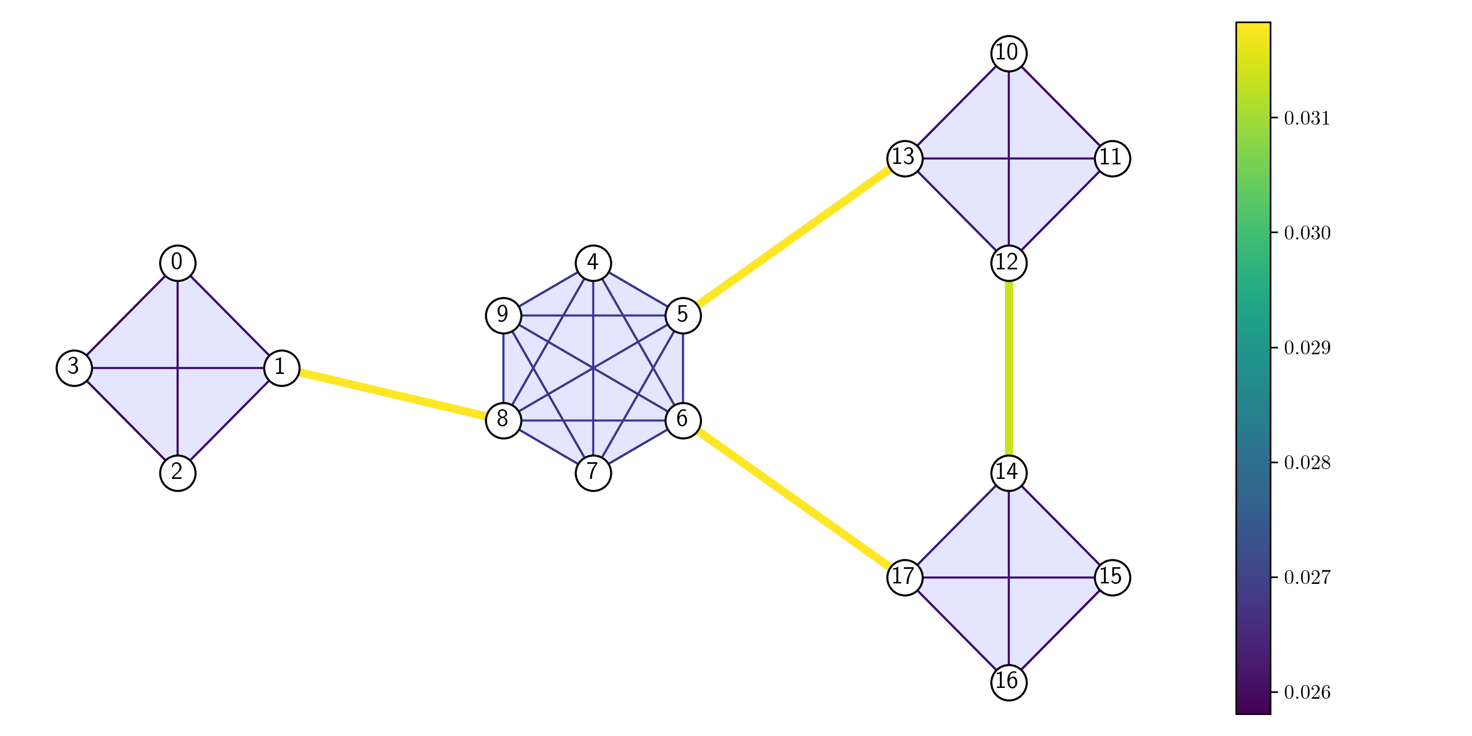
(c) Edge PageRank

Figure 1.1: Comparison of graph-based centrality measures (a–b) to the Edge PageRank measure (c). The top four edges of each centrality are bolded in the left plots (five in the case of betweenness centrality, due to a tie). (a) Betweenness centrality equally weights shortest paths across the entire network, such that $\{5,8\}$ is considered more bridging than $\{12,14\}$, even though the former is embedded in a clique and is unlikely to be between unlike individuals in practice. (b) The PageRank measure, a standard measure of importance in graphs, can be applied to the line graph transformation of the graph  to define a measure of importance on edges Easley and Kleinberg (2010). However, instead of measuring whether a tie is bridging, the measure is influenced by the size of the communities and transitive closure, resulting in edges such as $\{5,6\}$ considered weaker than $\{1,8\}$. (c) Edge PageRank centrality clearly identifies the bridges in the network, which are likely to be conduits for novel information and provide access to important network resources.

We conduct large-scale experiments on seven datasets that illuminate the role of higher-order interactions in identifying global and local bridges in a network, reflecting its ability to formalize and distinguish between different types of topological holes. Global bridges are edges whose removal will disconnect the network, whereas local bridges are edges whose end points have no common connections. This distinction between types of bridges, which can not be made by previous measures such as embeddedness (Granovetter 1985) or the network constraint measure (Burt 2002), is important in population-scale studies of social networks (Reagans and McEvily 2003, Park et al. 2018). We show that the Edge PageRank measure effectively finds and distinguishes between types of bridges in social networks when compared to existing measures, supporting its use as a measure of the extent to which a relationship acts as a bridge.

The second part of our approach uses the concept of Hodge Decomposition Hatcher (2002) to better understand the connection between dyadic tie strength and network structure. Hodge Decomposition enables the analysis of flows by decomposing any flow defined on the edges of a simplicial complex as the sum of three components: a curl component reflecting a “vorticity” of flow, a gradient component reflecting “disagreement” between nodes, and a harmonic component reflecting topological “obstructions” of the network. Roughly, the curl component of a flow is supported on edges which take part in triangles, the gradient component is the part of the flow which sums to zero around cycles, and the harmonic component is the remainder of the flow (see Section 2 for formal definitions). We show that this topological definition has the following sociologically relevant associations: that a high curl component can be associated with flows on edges which are incident to many triangles (i.e., those edges with a high edge degree), a high gradient component can be associated with flows that are supported on global bridges, and that the harmonic component can be associated with flows that are supported on local bridges. In regressing the curl, gradient, and harmonic components of Edge PageRank flows on proxies for tie strength, we find that the coefficients of curl and gradient components are larger than that of the harmonic component.

As a result, we are able to replicate and explain the “U”-shape relationship between tie strength and tie range observed by Park et al. (2018). Namely, for non-bridging ties, we show that the curl component of Edge PageRank is positively associated with dyadic tie strength, which is consistent with Granovetter’s “Forbidden Triad.” For bridging ties, we find that the gradient component of Edge PageRank is more positively associated with tie strength than the harmonic component, which recovers the “U”-shape noted by Park et al. (2018) as low span local bridges are more likely to be associated with the harmonic component of Edge PageRank and high span local bridges and global bridges are more likely to be associated with the gradient component of Edge PageRank. This ultimately suggests that individuals implicitly understand the value of a bridging tie with respect to the hole that it spans in network structure.

Our approach is evaluated on nine large-scale empirical datasets of diverse social interactions, including physical proximity contacts, emails, and text messages. Each dataset provides auxiliary information, such as the frequency of interactions, that we use to generate (approximately) continuous measures of tie strength for each edge. We find that Edge PageRank more effectively captures tie strength than dyadic measures such as embeddedness. Altogether, our results show that restricting to the graph-based representations of networks results in a loss of potentially critical information for identifying socially relevant features of a network. By incorporating higher-order information from group interactions, our approach provides a novel and empirically valuable methodology which captures the nuances of recent empirical work.

Organization

The rest of the paper is organized as follows. We begin with a discussion of preliminaries in Section 2 where we formally introduce the Edge PageRank measure as originally defined in Schaub et al. (2020) and the Hodge Decomposition. In Section 3 we make explicit the way in which the Edge PageRank measure identifies bridging relationships and describe how Hodge Decomposition can explain dyadic tie strength. In Section 4, we then discuss the empirical data and methodology used to support our results. Section 5 displays the results of our empirical analysis, where we discuss how Edge PageRank empirically identifies bridging relationships and how the Hodge Decomposition clarifies the relationship between bridging relationships and dyadic tie strength. We summarize our findings and contributions in Section 7.

2 Preliminaries

In this section we formally define relevant concepts from algebraic topology. First, we describe simplicial complexes, the primary data structure used to model our network data, and Hodge Laplacians, which are a key mathematical structure used to analyze simplicial complexes. We show how the Edge PageRank measure of Schaub et al. (2020) can be defined through a normalized Hodge Laplacian, and then introduce the tool of Hodge Decomposition. In this manuscript, we mainly focus on the case where the network data consists of group interactions with size at most three. In the Supplementary Information, we generalize these mathematics to allow for larger group interactions, and provide additional illustrative examples.

Simplicial Complexes

Most network models of social interaction make use of a graph $G=(V,E)$, where $V$ is a set of nodes representing individuals and $E\subseteq\binom{V}{2}$ is a set of pairwise interactions between individuals. Here, we will consider a simplicial complex $\mathcal{X}\subseteq 2^{V}$, where $V$ is again a set of nodes, but now $\mathcal{X}$ can model relationships of arbitrary size.

As an illustrative example of how a simplicial complex has more representational power than a graph, take the setting of co-authorship. Consider two scenarios: First, where authors $A$, $B$, and $C$ all coauthor a paper with one another, and second, where $A$ and $B$ coauthor one paper, $B$ and $C$ coauthor a different paper, and $A$ and $C$ coauthor a third separate paper. In both scenarios, a graph would model the network data as a clique between $A$, $B$, and $C$. However, a simplicial complex could distinguish between the first scenario and the second, as in the first we would have $\{A,B,C\}$ in the complex but in the second we would not.

A simplicial complex has the following structural property:

$$\sigma\in\mathcal{X}\implies x\in\mathcal{X}\,,\qquad\forall x\subseteq\sigma\,.$$

That is, for every simplex $\sigma$ which belongs to the simplicial complex $\mathcal{X}$, every subset of $\sigma$ (denoted $x$ in the equation above) must also be in the simplicial complex $\mathcal{X}$. In the context of this work, this property implies that for every triangle $\{u,v,w\}\in\mathcal{X}$, each associated edge ($\{u,v\}$, $\{u,w\}$, and $\{v,w\}$) is also in $\mathcal{X}$. This simple structural property is ultimately powerful as it leads to many important mathematical results on simplicial complexes (see, e.g. Hatcher (2002)) and allows us to formally define Hodge Laplacians.

Hodge Laplacians

Hodge Laplacians, also referred to as Eckmann Laplacians (Eckmann 1944), are a set of matrices which generalize the notion of the graph Laplacian, a core mathematical object in spectral graph theory (Chung 1997, Hatcher 2002). These matrices are defined using boundary operators, presented briefly here and discussed in full in the Supplementary Information.

Here, we focus on two types of boundary operators which are relevant to our data. The node-edge boundary operator $B_{1}\in\mathbb{R}^{n\times e}$ and the edge-triangle boundary operator $B_{2}\in\mathbb{R}^{e\times t}$ (recall that in our notation we have $n$ nodes, $e$ edges, and $t$ triangles in the data). For each edge $\{u,v\}$ in the complex, with $u<v$ without loss of generality, the operator $B_{1}$ has a $+1$ in the entry corresponding to the column for node $u$ and the row for edge $\{u,v\}$, and a $-1$ in the entry corresponding to the column for node $v$ and the row for edge $\{u,v\}$. Similarly, for each triangles $\{u,v,w\}$ in the complex, with $u<v<w$, the operator $B_{2}$ has three entries in the row corresponding to $\{u,v,w\}$: 2 entries which are $+1$ in the columns corresponding to $\{u,v\}$ and $\{v,w\}$, and a $-1$ in the column corresponding to $\{u,w\}$.

This choice for signs of entries in the above operators guarantees that $B_{1}B_{2}=0$, which reflects the idea that the boundary of a boundary is null. Equivalently, the condition states that the image of the operator $B_{2}$ is contained in the kernel of the operator $B_{1}$, which motivates the study of the $1$-Hodge Laplacian (Hatcher 2002).

Definition 1 ($1$-Hodge Laplacian).

The $1$-Hodge Laplacian is a matrix $L_{1}\in\mathbb{R}^{e\times e}$ defined:

$$L_{1}=B_{1}^{\top}B_{1}+B_{2}B_{2}^{\top}\,.$$

As discussed in the Supplementary Information, the definition above is a specific instantiation of the $k$-Hodge Laplacian $L_{k}=B_{k}^{\top}B_{k}+B_{k+1}B_{k+1}^{\top}$, where $B_{k}$ and $B_{k+1}$ represent arbitrary boundary operators. $L_{0}=0+B_{1}B_{1}^{\top}$ recovers the familiar graph Laplacian, so $L_{1}$ can be thought of as a natural extension of the graph Laplacian to define an operator on edges. Notably, while the dimension of the null space of $L_{0}$ corresponds to the number of connected components in a graph, the dimension of the null space of $L_{1}$ corresponds to the number of one-dimensional topological holes in a simplicial complex, i.e. cycles in the complex which are not filled with triangles.

Importantly, Schaub et al. (2020) showed that there is a way to normalize the $1$-Hodge Laplacian such that it can be associated with a stochastic process

Definition 2 (Normalized $1$-Hodge Laplacian (Schaub et al. 2020)).

The normalized $1$-Hodge Laplacian is a matrix $\mathcal{L}_{1}\in\mathbb{R}^{e\times e}$ defined

$$\mathcal{L}_{1}=D_{2}B_{1}^{\top}D_{1}^{-1}B_{1}+B_{2}D_{3}B_{2}D_{2}^{-1}\,,$$

where $D_{1}$, $D_{2}$, and $D_{3}$ are normalization matrices defined in the Supplementary Information.

Schaub et al. (2020) show that the normalized $1$-Hodge Laplacian corresponds to a random walk in a “lifted space.” Specifically, they show that the normalized $1$-Laplacian is related to a stochastic matrix $\widehat{P}\in\mathbb{R}^{2e\times 2e}$, where $\widehat{P}$ describes a walk on a lifted graph where each node corresponds to one of the orientations of each edge (e.g., for the edge $\{1,2\}$, the lifted graph has one node for $[1,2]$ and another for $[2,1]$). Formally, the relationship between $\mathcal{L}_{1}$ and $\widehat{P}$ is as follows:

$$-\frac{\mathcal{L}_{1}}{2}V^{\top}=V^{\top}\widehat{P}\,,$$ (1)

where $V=\begin{bmatrix}I_{e}\\ -I_{e}\end{bmatrix}$ is referred to as a lifting operator. Equivalently, by right multiplying each side of the inequality by $-V$, we can write $\mathcal{L}_{1}=-V^{\top}\widehat{P}V$, which implies that the operator $\mathcal{L}_{1}$ on a vector $x$ can be interpreted as a sequence of three operations:

1. First, $x$ is lifted into a $2e$ dimensional space, $Vx\in\mathbb{R}^{2e}$.

2. Then, $\widehat{P}$ acts on the lifted vector, $\widehat{P}Vx\in\mathbb{R}^{2e}$.

3. Finally, the operator $-V^{\top}$ projects this output back into the $e$-dimensional space, so $\mathcal{L}_{1}x=-V^{\top}\widehat{P}Vx\in\mathbb{R}^{e}$.

In Section 3, we provide more detail on how to interpret this random walk and lifting procedure as a way to identify bridging relationships.

Edge PageRank

The random walk in the lifted space associated with the normalized $1$-Hodge Laplacian can be used to generalize the standard notion of PageRank from Page et al. (1999) to a define PageRank on edges. Specifically, the random walk from the matrix $\widehat{P}$ discussed above is augmented with a teleportation step, where the random walker either follows the walk in $\widehat{P}$ with some probability $\alpha$ or teleports with a probability $1-\alpha$. The Edge PageRank vector can ultimately be defined as a function of the $1$-Hodge Laplacian, where $\beta=2/\alpha$.

Definition 3 (Edge PageRank (Schaub et al. 2020)).

Let $\mathcal{X}$ be a simplicial complex with normalized Hodge Laplacian $\mathbf{\mathcal{L}}_{1}$, $\mathbf{x}$ be a vector of the form $\mathbf{x}=\mathbf{V}^{\top}\mathbf{\mu}$ where $\mathbf{\mu}$ is a probability vector, and $\beta\in(2,\infty)$. The Edge PageRank vector $\boldsymbol{\pi}_{1}$ is defined as the solution to the linear system

$$(\beta\mathbf{I}+\mathbf{\mathcal{L}}_{1})\boldsymbol{\pi}_{1}=(\beta-2)\mathbf{x}\,.$$ (2)

In this work, we will consider personalized Edge PageRank vectors, where $\mathbf{x}$ in the definition above has one entry equal to 1 and the rest equal to 0. We restrict to this case for interpretability of results.

Hodge Decomposition

(a) Original Flow, $\mathbf{x}$

(b) Gradient Component. $\mathbf{x}^{g}$

(c) Curl Component, $\mathbf{x}^{c}$

(d) Harmonic Component, $\mathbf{x}^{h}$

Figure 2.1: Example of an (unnormalized) Hodge decomposition of a flow on a simplicial complex. Gradient flows sum to 0 around cycles: these flows are associated with global bridges in a network, as global bridges can not be a part of a cycle. Curl flows are non-zero around triangles and 0 elsewhere, and we associate these flows with strong ties as empirical data suggests strong ties tend to take part in triangles. Harmonic flows sum to 0 around triangles but are non-zero around longer cycles, and hence are associated with local bridges, which are always part of such longer cycles.

The normalized Hodge Laplacian can be used to decomposed any vector in $\mathbb{R}^{e}$ three orthogonal components. Here, we present the the unnormalized Hodge decomposition associated with $L_{1}$ and discuss the normalized Hodge Decomposition in the Supplementary Information. Because $B_{1}B_{2}$ = 0, we have that every vector $\mathbf{x}\in\mathbb{R}^{e}$ can be decomposed into orthogonal components as follows

$$\mathbf{x}=\mathbf{x}^{g}+\mathbf{x}^{c}+\mathbf{x}^{h}$$ (3)

where $\mathbf{x}^{g}$ is the projection of $\mathbf{x}$ onto im($\mathbf{B}_{1}^{\top}$), $\mathbf{x}^{c}$ is the projection of $\mathbf{x}$ into im($\mathbf{B}_{2})$, and $\mathbf{x}^{h}$ satisfies $\mathbf{L_{1}}\mathbf{x}^{h}=0$. The importance of the Hodge Decomposition is in its interpretability, as it allows for different components of a flow on edges to become more clear. The interpretation of this decomposition is as follows, and each component is illustrated in Figure 2.1.

• im($\mathbf{B}_{1}^{\top}$) is the cut space of the edges. This subspace can be seen as the linear combinations of simplices whose cyclic components are zero. In this sense, $\mathbf{x}^{g}$ is a gradient flow between two nodes, as it corresponds to flows that have a (weighted) sum of 0 around cycles.

• im($\mathbf{B}_{2})$ is made of the flows that can be described via local circulations along triangles. $\mathbf{x}^{c}$ is a circulation around a filled triangle in the graph and can be seen as a curl flow.

• $\ker(L_{1})$ can be seen as a space of flows which are orthogonal to those described above. Hence, such flows are locally consistent around $2$-simplices, but are globally inconsistent around longer cycles.

Ultimately, we are able to show that this set of mathematical tools has sociological relevance, as discussed in the following section.

3 Identifying Bridging Relationships with a Stochastic Process

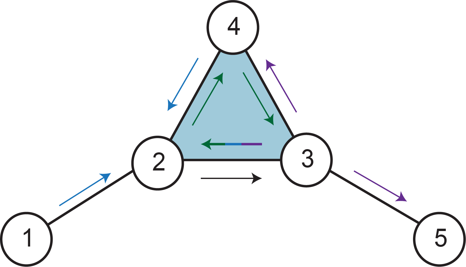
Figure 3.1: Illustration of the random process underlying Edge PageRank. Each state of the process corresponds to a directed edge, which we interpret as passed messages. If the state of the random walk is currently $[2,3]$ (black), i.e. $2$ has just sent a message to $3$, then there are 3 possible types of steps that can be taken next. The lower walk (purple) indicates that, after $3$ receives a message, then $3$ may send a message to one of its neighbors, including $2$. This walk is designed to be reversible (blue), to create a desirable symmetry for the Edge PageRank measure. The upper walk (green) represents the effect of higher order information in the process. Once $2$ sends a message to $3$, then $2$ can send a message to $4$, indicating that a message is being sent to both members of the simplex, or $4$ might send a message to $3$, indicating that after $4$ sees a message sent from $2$ to $3$, node $4$ may take the action to communicate with node $3$. In the third possible transition, the walk may teleport to a pre-determined seed message (not shown).

In this section, we describe Edge PageRank as a stochastic process contextualized in terms of information exchange whose equilibrium corresponds to the Edge PageRank scores. We note that this stochastic process naturally identifies bridging relationships, in the sense that ties with large scores are likely to span structural holes in the network.

The Information Exchange Process

Sociologists point out that any measure of centrality on a social network can be understood through an underlying social process (Friedkin and Johnsen 1990), and here we show this to be true for the Edge PageRank measure (Schaub et al. 2020). The “states” in our stochastic process are given by the two possible directions that information could flow along each edge. Formally, each edge between individuals $A$ and $B$ can result in two states for the process: $A$ sending a message to $B$, or $B$ sending a message to $A$, denoted $[A,B]$ and $[B,A]$, respectively. The process “walks” (transitions or moves) between these discrete states randomly. Hence, the random walk corresponds to a (random) series of messages being sent throughout the network, and Edge PageRank will be a function of the steady-state distribution of this random walk.

The transitions between states of the random walk are based on three possible types of transitions: a lower walk, an upper walk, and a teleportation maneuver (Figure 3.1). The lower walk represents a standard local information exchange in a graph, where after an individual receives a message, then they send a message to one of their neighbors. That is, if the state is $[A,B]$, the next state in the lower walk is of the form $[B,C]$ where $C$ is connected to $B$. For symmetry, the lower walk goes in both directions, so that if the state is $[B,C]$, the next state of the random walk can return to $[A,B]$.

The upper walk incorporates the higher order (group) information of the network. If $A$ has just sent a message to $B$, and $A,B,$ and $C$ are a part of a triangle, then the upper walk would allow two additional possible states for the next message. In the first, $A$ sends a message to $C$, emulating a group conversation in which $A$ has said something to both $B$ and $C$. In the second additional state, $C$ sends a message to $B$, indicating that due to the higher-order structure, $C$ has seen the message which has just passed from $A$ to $B$, and can act on this to communicate with $B$.

These higher order steps from the upper walk allow the property of simplicial closure, the generalization of triadic closure to group interactions (Benson et al. 2018), to manifest itself in the measure of tie strength. Edges which take part in triangles to have more communication flow through them in the opposite direction of the lower walk, as is explicit in Figure 3.1 where the steps of the upper walk are in direct opposition to those of the lower walk. This opposition represents a “vorticity” due to higher order information, and is a common observation in analyses of networks with higher order interactions (Lim 2020).

The final possible transition in the social process is a teleportation step. In this step, independent of the preceding state of the random walk, the state “teleports” to a pre-specified seed message from one particular node to another. Because the teleportation step requires a particular seed edge, we refer to the outcome of the process as personalized Edge PageRank, such that each Edge PageRank computation is specific to a particular choice of seed message.

This teleportation step is required for the stochastic process, due to the way in which the centrality measure takes differences between the two probabilities on each edge in order to define a centrality. Namely, because of the symmetry in the underlying stochastic process due to the reversibility of the lower walk and symmetry in the upper walk, without the teleportation step the differences along edges would become 0. This symmetry of the random walk also requires us to use personalized Edge PageRank, as opposed to the standard formulation of PageRank which uses a teleportation step which is uniform across all possibilities. If the process were to use a uniform teleportation step, then all messages in the random walk would have the same steady-state probability as the messages in the opposite direction, resulting in values on each edge which are identically 0. Taking differences in between the two probabilities on each edge is crucial to the sociological implications of the measure. Namely, taking differences aids the identification of bridging relationships because it highlights limitations in communication which are typical of bridging ties (Aral and Van Alstyne 2011, Reagans and McEvily 2003).

Once a steady-state distribution for the stochastic message passing process is computed and differences are taken across each edge, the final step in developing a centrality measure is to assign a value to each edge. To do so, we compute the total size of the vector by using the $2$-norm of each personalized Edge PageRank vector, which is intended to capture the diffusion of the Edge PageRank vector across the edges of the simplicial complex. For a specific choice of seed messages, this operation highlights the presence of edges along which there is asymmetry in the communication flow defined by the stochastic process, as larger asymmetries result in higher difference values and hence larger sizes of the Edge PageRank vector. Further, using the size of the vector allows the computed values to be independent of which orientation of the edge is used for the seed message, i.e. whether the seed is $[A,B]$ or $[B,A].$

Identification of Bridging Ties

The primary features which allow Edge PageRank to identify bridging ties are two-fold. First, the use of differences in summarizing the outcome of the stochastic process allows the measure to highlight ties along which messages flow in one direction but not the other. This inability for communication to flow easily along both directions is common to the study of bridging ties, as their position in the network makes communication particularly difficult (Aral and Van Alstyne 2011, Reagans and McEvily 2003). Roughly, because bridging ties are often between individuals with different backgrounds or who belong to different communities, communication is often limited when compared to strong ties (Aral and Van Alstyne 2011). In the defined stochastic process, this bandwidth limitation of bridging ties is reflected by the inability of communication in the stochastic process to easily pass through both orientations of an edge, causing an asymmetry.

Second, the transitions in the stochastic process make it such that the presence of triangles in the data results in more symmetric communication along edges which take part in triangles. As noted previously, this is explicit in Figure 3.1 as the green arrows of the upper walk are in opposing directions to the blue and purple arrows of the lower walk. In this sense, we say that the stochastic process discounts the effect of triadic interactions. That is, the upper walk allows triangles in social networks to manifest themselves by allowing more avenues for communication within the network, in such a way to reduce the asymmetries of communication flows. Hence, if the seed edge in the personalized Edge PageRank computation takes part in many triangles, we would expect communication to be more symmetric along the seed edge compared the case in which the seed edge bridges between communities.

Hodge Decomposition

One of the benefits of using the simplicial complexes as a model of networks is that we can utilize the result of the so-called Hodge decomposition. Empirically, we find that this decomposition provides valuable information for identifying the tie strength of a particular relationship. Whereas before we summarized personalized Edge PageRank for an edge in a single value, the $2$-norm of the Personalized Edge PageRank vector, the Hodge Decompsition allows us to obtain a refined picture of the role of an edge by taking the $2$-norm of the curl, gradient, and harmonic components of the Edge PageRank vector. By computing the size of each of these components, we get an additional triplet of information which provides a concise yet nuanced perspective on each edge in the network.

We first use the Hodge Decomposition to strengthen the argument that Edge PageRank can identify bridging ties. In the Supplementary Information, we provide mathematical justification which shows that the Hodge Decomposition can be used to identify both local and global bridges in a network. Global bridges refer to edges whose removal disconnects the graph and local bridges refer to edges whose removal increases the length of the path between the two nodes the local bridge was a part of by at least 3. Global bridges hence span across “holes” in a network in the sense that they bridge two connected components within a network. In this way, the distinction between global and local bridges reflects a difference in the shape of a topological hole. As we show in the Supplementary Information, the gradient component of the Hodge Decomposition can be associated with global bridges (Supplementary Information, Proposition 1), and the harmonic component of the Hodge Decomposition can be associated with local bridges (Supplementary Information, Proposition 2).

In Section 6, we will discuss how the empirical evidence of this work suggests that the Hodge Decomposition can be used to disentangle a tie’s place in network structure from the dyadic strength of the tie. We show that the harmonic component of the personalized Edge PageRank of a tie is undervalued relative to the curl and gradient components of the Edge PageRank measure, replicating and explaining the empirical result of Park et al. (2018).

A Note on Computation

Additional higher-order interaction data gives rise to an increase in computational demands. For a simplicial complex with $n$ nodes, $e$ edges, and $t$ triangles, in the worst case the simplicial complex may be constructed in time $O(e^{3/2})$, although many implementations are more efficient (Schaub et al. 2020). Once the simplicial complex is constructed, the Personalized Edge PageRank vector can be computed in time $O(n^{2}e+e^{2}t)$, and solution techniques which utilize matrix sparsity can be used to increase the efficiency of the implementation (Schaub et al. 2020). Ultimately, this results in algorithms which run in time that is polynomial in the input size $n+e+t$, which can efficiently be applied to identify tie strength and structural holes in social networks.

4 Empirical Setting

4.1 Data

Table 4.1: Summary statistics for datasets used in tie strength experiments

dataset	nodes	edges	triangles	edge density
contact-primary-school	242	8,317	5,139	2.85e-01
contact-high-school	327	5,818	2,370	1.09e-01
contact-university	692	79,530	436,298	3.32e-01
email-Enron	144	1,344	1,159	1.31e-01
email-Eu	986	16,064	27,655	3.31e-02
india-villages	1,774	294,626	314,768	1.87e-01
sms-a	30,278	42,882	1,581	9.36e-05
sms-c	11,714	17,050	1,114	2.49e-04
college-msg	1,899	13,838	5,403	7.68e-03

Table 4.2: Summary statistics of datasets used for bridge identification experiments.

dataset	nodes	edges	triangles	local bridges	global bridges	edge density
coauth-MAG-10	80,198	237,261	355,186	1,701	8,758	7.38e-05
coauth-ai-systems	27,488	86,994	100,902	952	2,310	2.30e-04
dbpedia-producer	32,383	93,342	184,694	2,749	9,421	1.78e-04
dbpedia-starring	61,727	668,459	2,885,569	5,392	2,959	3.51e-04
dbpedia-writer	65,165	335,125	1,385,303	581	5,241	1.58e-04
email-Eu	979	29,299	160,605	53	63	6.12e-02
genius-rap	47,167	128,808	215,049	6,057	16,471	1.16e-04

Our experiments use two categories of datasets: one set of datasets is used to validate that Edge PageRank identifies bridging relationships, and one set of datasets which are used for predicting the dyadic tie strength of particular relationships. The datasets used for tie strength prediction have some auxiliary proxy for tie strength, such as the frequency of interaction between two individuals (Granovetter 1973). We use this auxiliary information only for evaluation; the interaction data input to the method are given by the set of interactions without frequency information, i.e., an interaction between individuals is included if they interacted at least once. To validate that Edge PageRank identifies bridging relationships, we use the following social network datasets, where we validate that each network has at least 50 global bridges and at least 50 local bridges (see Table 4.2 for summary statistics).

• coauth-ai-systems, coauth-MAG-10. Nodes are computer science researchers and simplices correspond to multiple authors coauthoring a paper. The coauth-ai-systems dataset consists of articles from computer systems conferences (VLDB, SIGMOD) and machine learning conferences (AAAI, NeurIPS, ICML, IJCAI), from 2000 to 2016. The coauth-MAG-10 dataset is from ten large computer science conferences. Both datasets are based on the the Microsoft Academic Graph (Amburg et al. 2020, Sinha et al. 2015).

• email-Eu. Nodes are email addresses and a simplex is formed if individuals send or CC one another on emails within a week.

• genius-rap. Nodes are rap music artists and simplices are sets of rappers collaborating on songs (Benson et al. 2018).

• dbpedia-producer, dbpedia-writer, dbpedia-starring. Nodes are individuals, and simplices correspond to producer collaborations on creative works, coauthoring written works, and costarring in movies, respectively (Auer et al. 2007).

For tie strength experiments, we use the following networks (see Table 4.1 for summary statistics).

• contact-primary-school, contact-high-school, contact-university. Nodes are individuals, and simplices form when individuals are in proximity of one another within a short time period. Data comes from individuals at a primary school (Stehlé et al. 2011), a high school (Mastrandrea et al. 2015), and a university (Sapiezynski et al. 2019).

• email-Enron, email-Eu. Nodes are email addresses and a simplex is formed if individuals send or CC one another on emails within a week; the email-Eu dataset spans over 2 years of communication at a European research institute (Benson et al. 2018, Paranjape et al. 2017) (same as above), and the email-Enron dataset spans the lifetime of the American energy company Enron (Benson et al. 2018, Klimt and Yang 2004) .

• india-villages. Nodes are individuals in villages in India, and edges form between individuals based on survey data (Banerjee et al. 2013), and simplices correspond to individuals living in the same household.

• sms-a, sms-c, college-msg. Nodes are individuals, and a simplex forms between individuals if they all send a message to each other within a week (Wu et al. 2010, Panzarasa et al. 2009).

For all datasets except india-villages, tie strength is based on the number of times two individuals appeared in some interaction together. In other words, if two individuals are in contact frequently, then their tie is considered to be stronger. Since the distribution of frequency of contacts is heavy-tailed, we use the log of the frequency for tie strength in our experiments. For the india-villages dataset, tie strength is determined on a scale of 1 to 12 based on answers to a questionnaire take by each individual (Banerjee et al. 2013).

4.2 Methods

For experiments on bridges, we define the dependent variable $y_{e}$ categorically, as the edge is either a global bridge, a local bridge, or neither. For experiments, we take a sub-sample of the dataset to make sure each class of edges is equally represented. Then, using different sets of independent variables, we learn linear logistic regression model with a training set to generate a prediction $\widehat{y}_{e}$ based on different features of the edge based on network topology, as done for tie strength. For a test set $T$, accuracy is computed as $\frac{1}{|T|}\sum_{e\in T}\mathbf{1}(\widehat{y}_{e}=y_{e})$. The process is again repeated five times using $5$-fold cross validation, and the mean of the test accuracies and standard deviations are reported (see Table 5.1, Table B.3, and Table B.4).

For the experiments on tie strength, we denote the dependent variable as $s_{e}$, which is a real number which measures the tie strength of each edge, as defined in the previous section for each dataset. We then compute a set of independent variable for each edge based on the network topology, either using personalized Edge PageRank and/or its components, or baselines from the literature.

In all experiments, the teleportation parameter for Edge PageRank is set to $\alpha=2/2.5=0.8$ and for Node Pagerank baselines it is set to $\alpha=0.85$ to be consistent with previous literature (Page et al. 1999, Schaub et al. 2020). These independent variables are then used in a linear regression on a training set, which allows for estimates of tie strength $\widehat{s}_{e}$ to be computed for each edge. Then, on a test set of edges $T$, we compute $1-\frac{1}{|T|}\sum_{e\in T}(\widehat{s}_{e}-s_{e})^{2}$ as a measure of accuracy of the prediction. The process is repeated five times, where each time the training set consists of a disjoint set of edges comprising $1/5$ of the total dataset, i.e. we use $5$-fold cross validation. The mean of the test accuracies and standard deviations are reported (see Table 5.2 and Table B.1).

5 Results

Table 5.1: Accuracy in predicting if an edge is a global bridge, a local bridge, or neither. In all cases, Edge PageRank outperforms both betweenness and the network constraint measure Burt (2000) in the classification task.

Dataset Name	Edge PageRank	Betweenness	Network Constraint
cat-edge-MAG-10	0.83 ($\pm$0.007)	0.58 ($\pm$0.058)	0.71 ($\pm$0.014)
coauth-ai-systems	0.77 ($\pm$0.026)	0.51 ($\pm$0.097)	0.70 ($\pm$0.024)
dbpedia-producer	0.83 ($\pm$0.006)	0.45 ($\pm$0.081)	0.60 ($\pm$0.010)
dbpedia-starring	0.94 ($\pm$0.003)	0.58 ($\pm$0.018)	0.73 ($\pm$0.006)
dbpedia-writer	0.93 ($\pm$0.012)	0.58 ($\pm$0.014)	0.62 ($\pm$0.022)
email-Eu	0.92 ($\pm$0.015)	0.78 ($\pm$0.070)	0.86 ($\pm$0.050)
genius-rap	0.79 ($\pm$0.006)	0.55 ($\pm$0.076)	0.60 ($\pm$0.022)

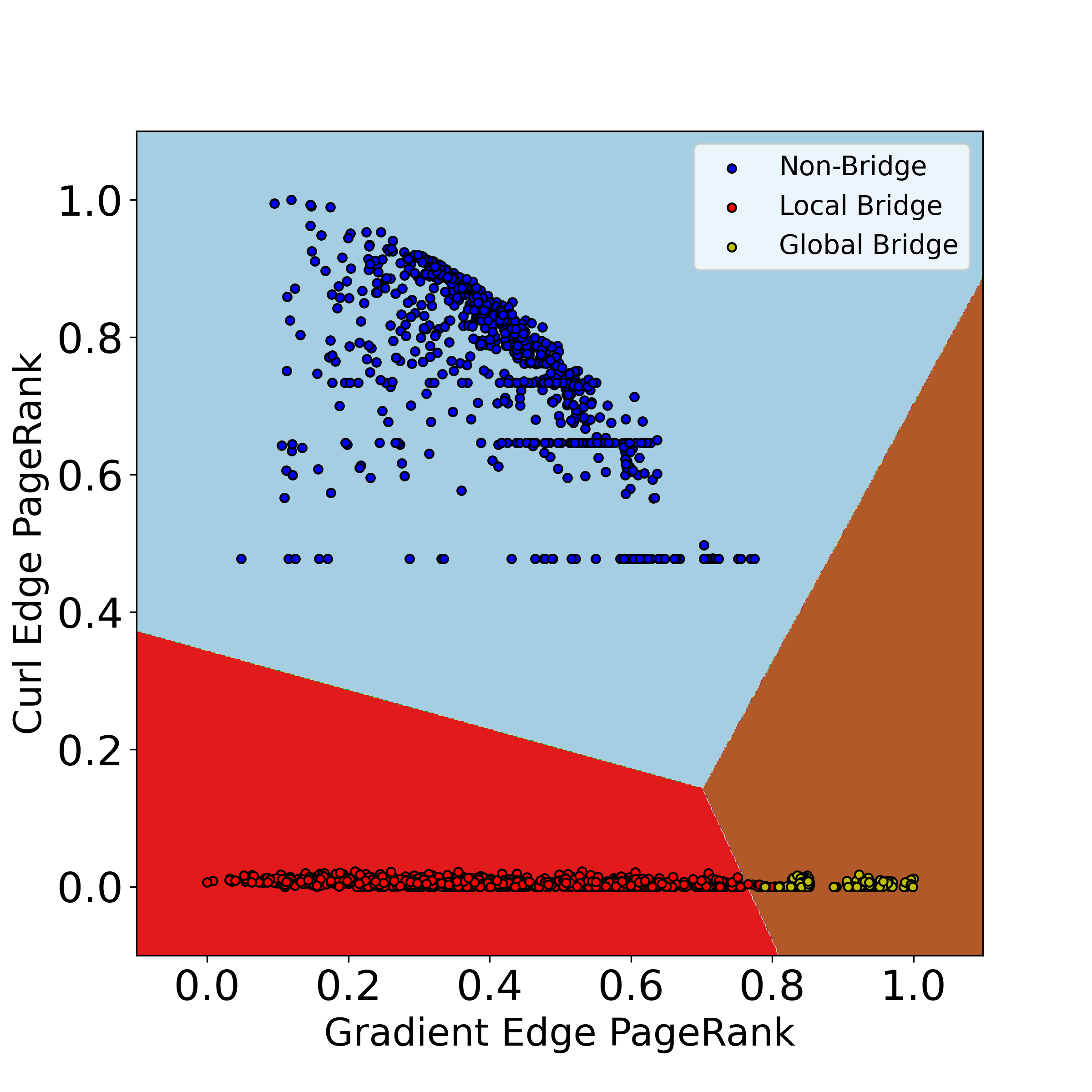
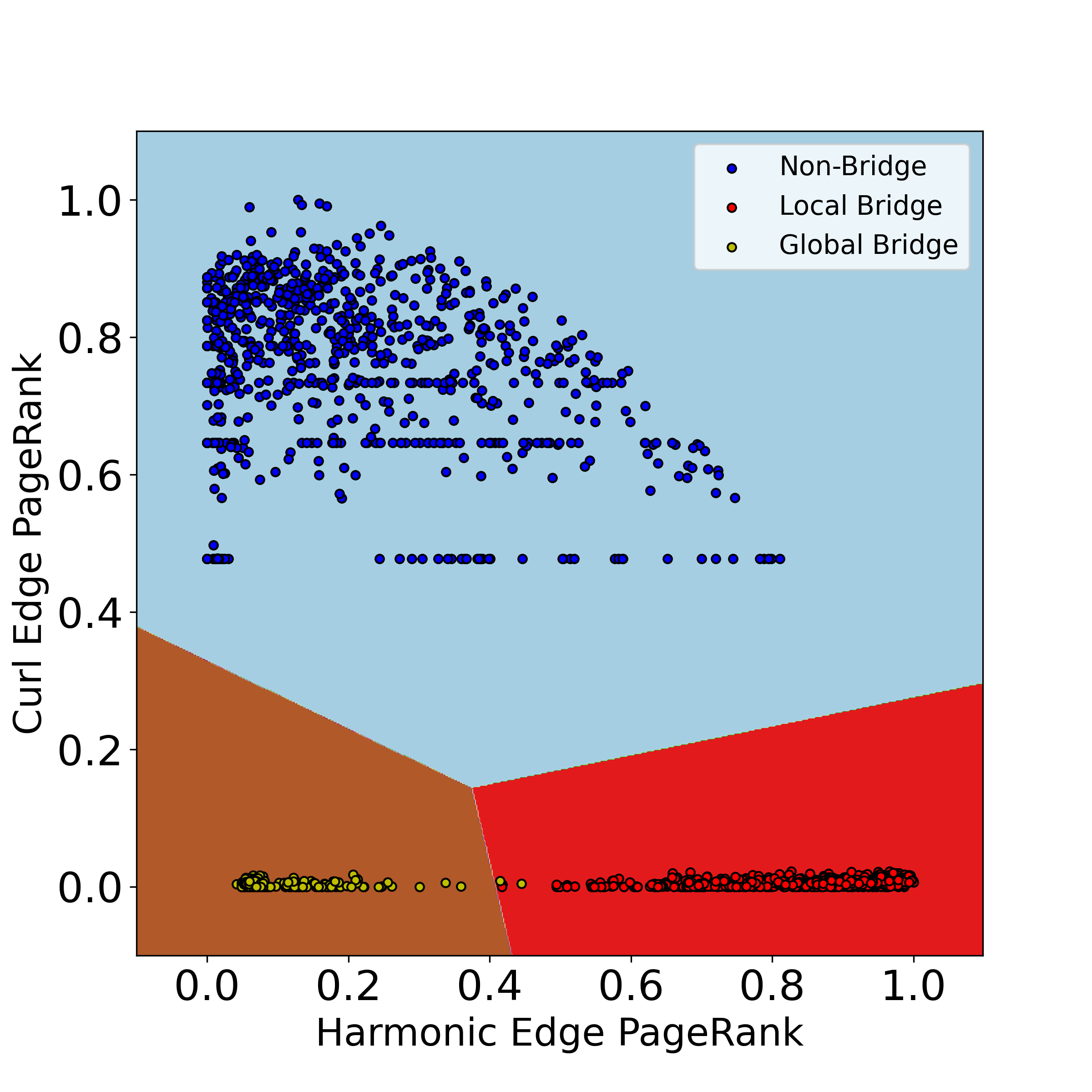
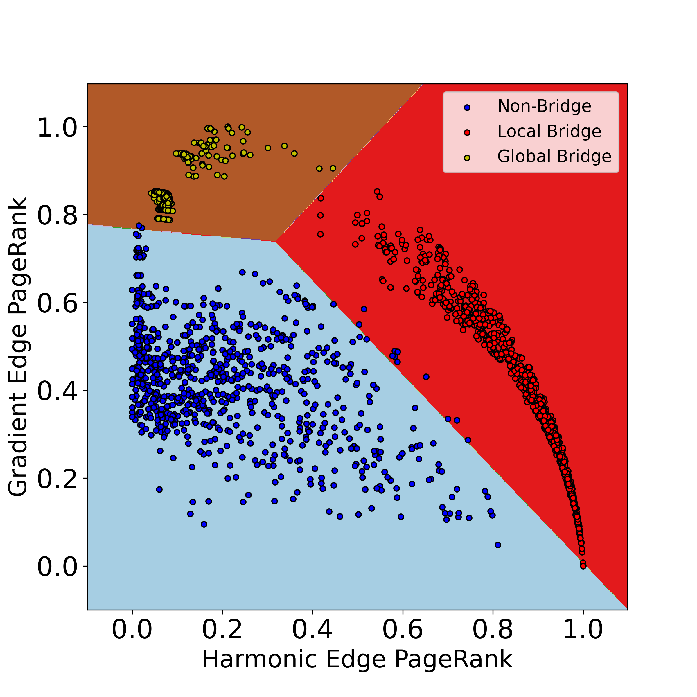
Figure 5.1: Decision boundaries of logistic regression using Edge PageRank components as regressors, illustrated for the couath-ai-systems dataset. In (a) and (b), the curl component of Edge PageRank determines if an edge is either type of bridge, and then the remaining component distinguishes between local and global bridges. In (c), we see a unique tradeoff between harmonic and gradient components of Edge PageRank in the decision process. In particular, these plots suggest that the local bridges with the lowest harmonic and highest gradient values correspond to the “most global” of the local bridges. This interpretation is supported by a $-0.55$ correlation between Harmonic Edge PageRank and tie range of local bridges, and a $0.56$ correlation between Gradient Edge PageRank and tie range of local bridges. Hence, empirically, the Edge PageRank components are able to identify the size of a structural hole, in the sense that they distinguish between edges based on their tie range.

5.1 Identifying Bridging Relationships with Higher Order Information

Local and global bridges satisfy a natural structural criteria for brokerage and are well known to facilitate the spread of novel information (Burt 2002). While bridges are not always weak ties in population-scale networks (Park et al. 2018), they are structurally important conduits for information. Organizational sociologists have found importance in distinguishing between global and local bridges, as local bridges in an organization can often be indicators of inefficient organizational practices, whereas global bridges better serve the role of providing novelty (Reagans and McEvily 2003). Identifying and distinguishing between local and global bridges helps to distinguish between different types of structural holes present in the social network.

In general, efficient algorithms for identifying local and global bridges are known, as global bridges can be found in time $O(n+e)$ and local bridges can be found in time $O(e^{3/2})$, where $n$ is the number of nodes in the network and $e$ is the number of edges. However, these definitions are combinatorial in nature in the sense that the only differentiation between types of local bridges are due to their tie range, which measures the length of the second shortest path between neighboring nodes (Park et al. 2018).

Hence, measures such as betweenness have been developed in order to better quantify the way in which edges act as a bridge between communities in a network (Girvan and Newman 2002). Similarly, the network constraint measure has been used to identify structural holes in a network, but can not distinguish between types of bridges as it only uses local information to determine the presence of a structural hole (Burt 2000).

Empirically, we find that Edge PageRank outperforms both betweenness and the network constraint measure in identifying and distinguishing between global and local bridges in the multi-class classification task (Table 5.1). Here, we use multi-class logistic regression to predict if an edge is a global bridge, a local bridge, or neither, using either the size of the Personalized Edge PageRank vector or betweenness as the feature for prediction. Accuracy is then reported using the $0/1$ classification loss (as discussed in Section 4). This result suggests that Edge PageRank may be a more appropriate measure for determining the extent to which an edge acts as a bridge, and reinforces that Edge PageRank provides a valuable way to identify and distinguish between structural holes.

The curl, gradient, and harmonic components are also particularly useful for this task, and in fact only two of the three components are required for near perfect classification (Supplementary Information, Table B.3). This is supported by the logistic regression decision boundary when two Edge PageRank components are used, as illustrated by the coauth-ai-systems dataset (Fig. 5.1). Moreover, we note that the decomposition on simpler vectors than the Edge PageRank vectors are also effective for bridge identification (Supplementary Information, Fig. B.1).

When using a single metric to identify and distinguish between types of bridges, as opposed to combinations individual Hodge components of the personalized PageRank vectors, we find that the $2$-norm of the Personalized Edge PageRank vector provides the best accuracy for the multi-class classification (Supplementary Information, Table B.4). As discussed previously, this ability of the personalized Edge PageRank vector is not unexpected, as its underlying stochastic process accentuates those edges who pass information from one community to another.

5.2 Higher Order Information Identifies Tie Strength

In this section, we first show that Edge PageRank and Hodge Decomposition can be used to identify tie strength with high accuracy, and can replicate the “U”-shape curve observed empirically by Park et al. (2018). In the following section, we interpret these results to show how these results suggest a simple revision to Granovetter (1973)’s idea of the Forbidden Triad to better explain the relationship between tie strength and network structure.

Table 5.2: Accuracy in predicting tie strength with different sets of regressor. Edge PageRank is consistently the most accurate, but the methods are more comparable for the messaging datasets.

Dataset Name	Edge PageRank Components	Embeddedness	Local Baseline	Node PageRank Variants
contact-primary-school	0.77 ($\pm$0.003)	0.39 ($\pm$0.007)	0.43 ($\pm$0.007)	0.16 ($\pm$0.008)
contact-high-school	0.61 ($\pm$0.004)	0.35 ($\pm$0.008)	0.37 ($\pm$0.009)	0.22 ($\pm$0.013)
contact-university	0.73 ($\pm$0.001)	0.42 ($\pm$0.002)	0.47 ($\pm$0.002)	0.36 ($\pm$0.003)
email-Enron	0.57 ($\pm$0.015)	0.36 ($\pm$0.016)	0.39 ($\pm$0.015)	0.28 ($\pm$0.016)
email-Eu	0.66 ($\pm$0.003)	0.54 ($\pm$0.005)	0.54 ($\pm$0.005)	0.46 ($\pm$0.007)
india-villages	0.52 ($\pm$0.001)	0.37 ($\pm$0.001)	0.34 ($\pm$0.000)	-0.01 ($\pm$0.001)
sms-a	0.73 ($\pm$0.001)	0.72 ($\pm$0.001)	0.72 ($\pm$0.001)	0.71 ($\pm$0.002)
sms-c	0.76 ($\pm$0.002)	0.75 ($\pm$0.003)	0.75 ($\pm$0.003)	0.75 ($\pm$0.003)
college-msg	0.57 ($\pm$0.004)	0.55 ($\pm$0.003)	0.55 ($\pm$0.003)	0.56 ($\pm$0.003)

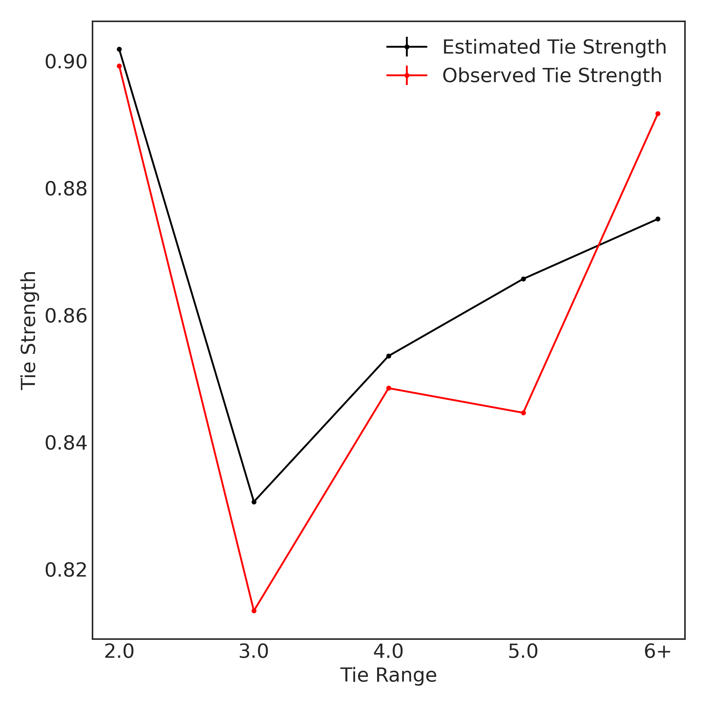
Figure 5.2: Estimated tie strength in the sms-c dataset as a function of tie range, when the Hodge Decomposition to predict tie strength. Here, tie range refers to the length of the second shortest path between two nodes. For the black line, we report the average predicted tie strength for all ties of a particular tie range, and standard deviation which is negligible. The red line reflects the same computation over the true values of tie strength as measured by the natural log of number of messages between two individuals. The strength of long ties noted in previous work (Park et al. 2018) is reflected in the data and captured by the Edge PageRank measure.

To assess the performance of Edge PageRank in identifying tie strength, we consider the following network-based baselines: embeddedness (i.e., number of common neighbors) (Gilbert and Karahalios 2009, Kossinets and Watts 2006, Marsden and Campbell 1984, Onnela et al. 2007), a set of three local measures identified by Mattie et al. as being predictive of tie strength (Mattie et al. 2018), and a set of regressors based on extending Node (standard) PageRank, namely the average of Node PageRank scores for each edge and Node PageRank scores on the line graph, and the same measures for $2$-norms of personalized Node PageRank vectors. These baselines are compared against using a combination of the three Hodge components of personalized Edge PageRank in order to predict tie strength. We use linear regression to predict tie strength using each set of features, and report the accuracy as $1-$ the mean squared error of the predictions compared to observed tie strength for each edge in dataset, as discussed in Section 4.

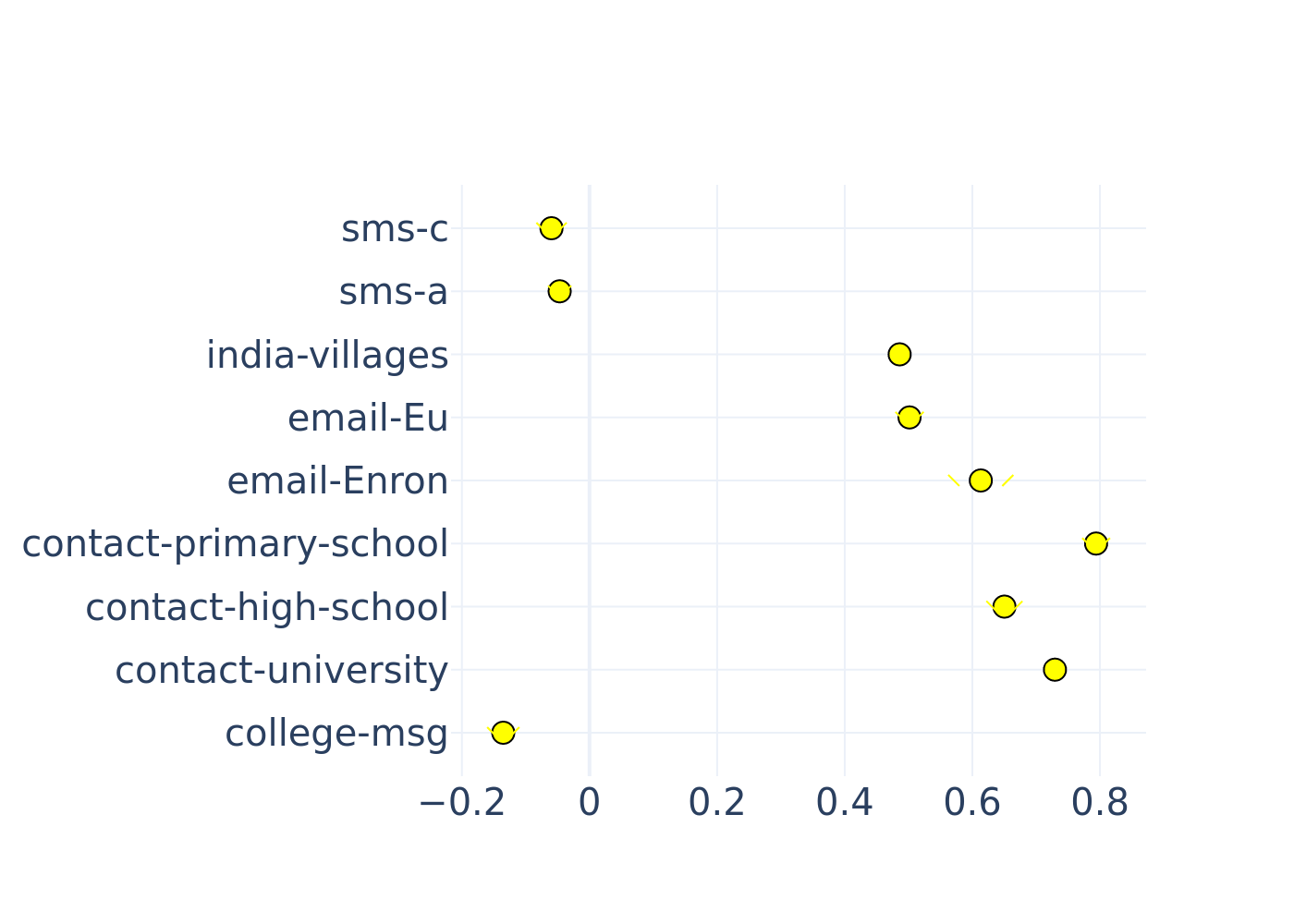
(a) Gradient Component

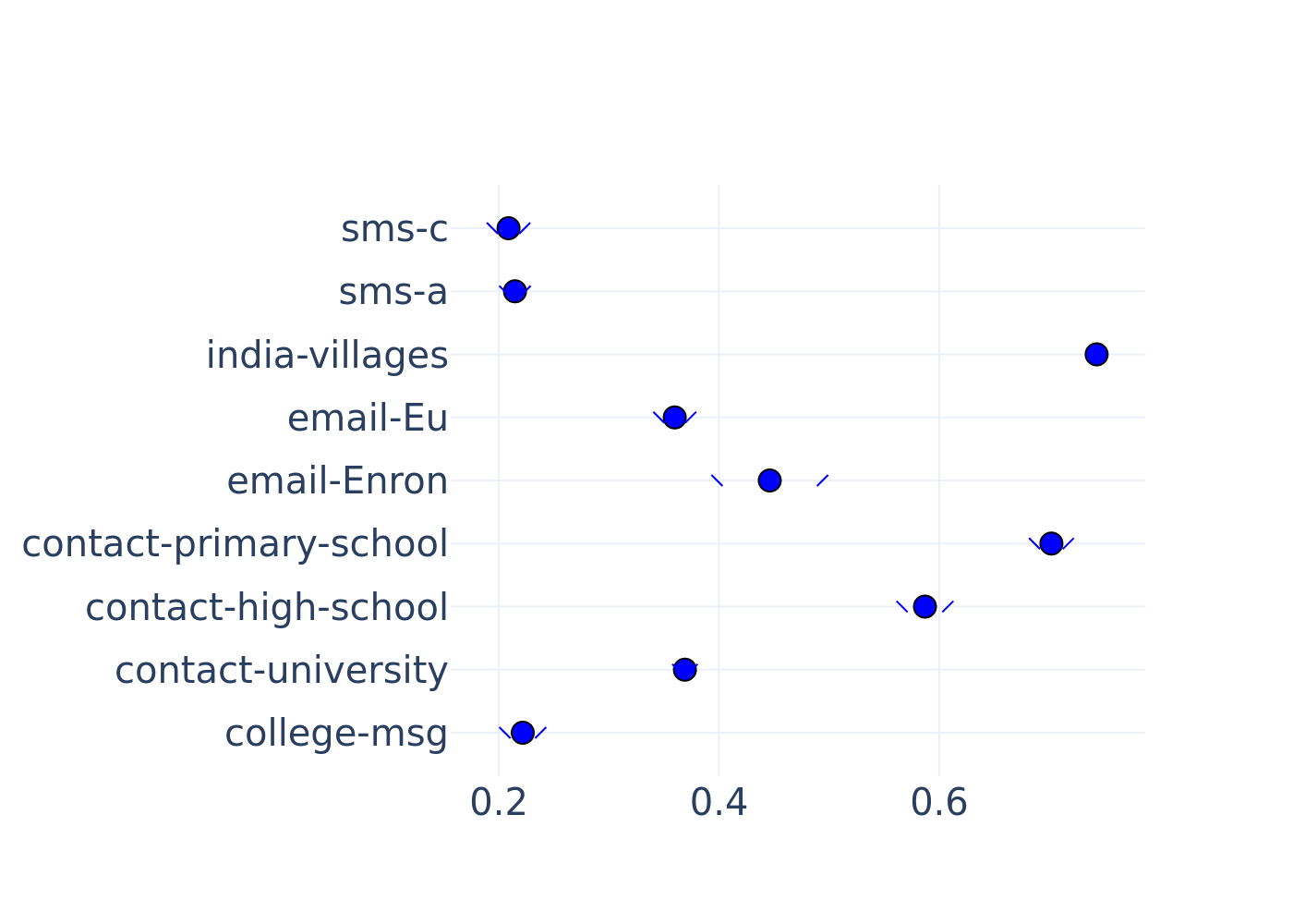
(b) Curl Component

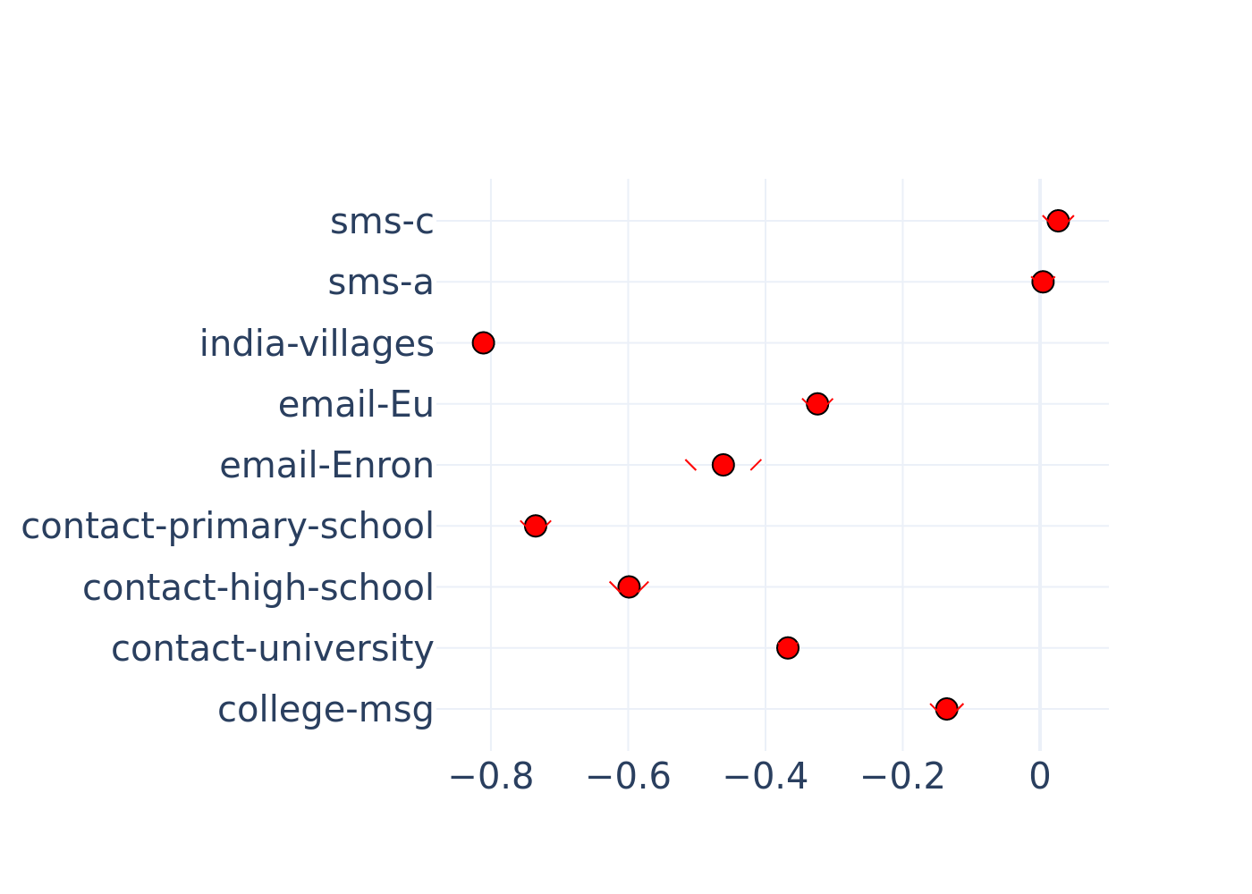
(c) Harmonic Component

Figure 5.3: Regression coefficients and 95% confidence intervals across datasets for individual components of Edge PageRank. A large harmonic component is indicative of weak ties, whereas large curl and gradient components are indicative of strong ties.

When restricting to a single measure for which to identify tie strength, we find that the size of the Personalized Edge PageRank vector, as opposed to the combination of individual Hodge components, appears to have the most consistent performance (Supplementary Information, Table B.1), outperforming network-based measures on datasets on the contact, email, and village datasets. The various methods have comparable accuracy on the messaging datasets.

We also measured the predictive power of each Edge PageRank component (curl, gradient, and harmonic) on tie strength. Through regressions on each individual component, we find that the harmonic component of Edge PageRank tends to be indicative of weak ties, whereas large curl and gradient components tend to indicate that a tie is strong (Figure 5.3).

Finally, part of the motivation for Edge PageRank was that the method can incorporate higher order interactions directly, under the assumption that higher order information should be informative. To support this, in the Supplementary Information, we report results from additional experiments on our datasets where higher order information is subsumed by pairwise information. That is, we fill in every triangle formed in the social network by pairwise interactions with a three-way higher order interaction. In this modified dataset, Edge PageRank is much less accurate in predicting tie strength (Supplementary Information, Table B.2), indicating that triads formed via higher-order interactions provide crucial data in identifying the strength of a tie.

6 Discussion

The results of the preceding sections suggest two important contributions to the literature: First, that the Edge PageRank measure is a valuable measure of the extent to which a relationship acts as a bridge, and second, the results on tie strength provide a formal (algebraic topological) explanation for Park et al. (2018)’s observation that tie strength has a “U”-shaped relationship with tie range. Namely, individuals in a social network seem to exhibit an aversion to topological obstructions, i.e. bridging ties that correspond to short non-contractible cycles do not exhibit as much strength compared to non-bridging ties or bridging ties that act as graph cut points.

Identifying Bridging Relationships

Theoretically, the evidence in Section 3 suggests that Edge PageRank identifies edges which are positioned as bridges in a social network using a continuous measure. The theoretical evidence can be viewed as a form of content validity for using Edge PageRank as a proxy for whether a relationship is bridging, as it provides an interpretation of the measure consistent with identifying bridging relationships. Empirically, Section 4 provides a form of face validity in that the Edge PageRank measure identifies global and local bridges, which are often between dissimilar individuals. Taken together, we see that Edge PageRank can be viewed as a novel measure of the extent to which a relationship can be seen as bridging. Importantly, the measure has the ability to distinguish between local and global bridges, which is of key importance in organizational settings (Reagans and McEvily 2003). Edge PageRank can distinguish between local and global bridges using a continuous scale, offering a refinement on the measure of tie range used in the literature.

What differentiates this approach from prior ways of identifying bridges is the way Edge PageRank makes use of its stochastic process. Traditionally, centrality measures in networks based on walks scale proportionally with the number of walks going through an edge (in the case of betweenness) or the amount of time a random walker spends on a particular state. Here, because Edge PageRank uses a projection that takes a difference between random walks, it scales inversely with the number of triangles incident to an edge, allowing it to identify bridging relationships. This unique postprocessing of the stochastic process, which is a mathematically natural consequence of using the Hodge Laplacian and shown here to be of empirical value, provides an interesting avenue for further research in the study of stochastic processes on networks.

When are Bridges Weak Ties?

Our results also suggest that Edge PageRank and the Hodge Decomposition are a useful measure of tie strength in their own right. We can understand the results of Section 5 as suggesting a new theory behind the relationship between social network structure and dyadic tie strength, based on the empirical evidence that using higher order information to estimate tie strength results in superior performance compared to graph-based methods. Theoretically, Figures 5.2 and 5.3 offer a revision to Granovetter (1973)’s suggested relationship between network structure and tie strength which is consistent with Park et al. (2018)’s recent empirical result. Specifically, Figure 5.2 makes it clear that our results are able to replicate the results of Park et al. (2018) in that tie strength and tie range have a “U”-shaped relationship. Figure 5.3 then helps us to understand the cause of this relationship, by suggesting that individuals undervalue the harmonic flow corresponding to a tie compared to the curl and gradient flows.

The curl component of a flow, which is associated with triadic interactions, is valued relatively highly, as would be suggested by Granovetter’s idea of the “Forbidden Triad.” In this sense, we see the results presented here as a simple extension of Granovetter’s original ideas about the relationship between network structure and tie strength, as non-bridging ties are likely to be strong.

The extension of the theory comes from the data surrounding bridging ties. Our results indicate that the harmonic flows are not as positively associated with tie strength as gradient flows. Because harmonic flows are associated with local bridges and gradient flows are associated with global bridges (see Section 3, and Propositions Proposition 1  and Proposition 2), the data suggests that individuals undervalue local bridges which have low tie range and value local bridges with higher tie range which appear “more global.” Intuitively, this is saying that individuals implicitly understand that global bridges are more likely to have novel information than low tie range local bridges, and hence they value the bridges which have high or infinite span. Stated another way, individuals are “hole-avoidant,” in the sense that information from low tie range local bridges is likely available from closer neighbors with whom one shares triadic interactions.

That is, we can view the curl component of Edge PageRank as capturing the social psychological motivations for a tie being strong (c.f. Krackhardt et al. (2003)), the gradient component of Edge PageRank as capturing the novelty of information which may come from an edge, which in turn motivates an individual to invest in the tie (c.f. Burt (2000), Jackson (2020)), and the harmonic component of Edge PageRank as an obstruction to both. As a result, the bridges which are weak ties are the ones which are most closely associated with topological obstructions from one-dimensional holes (i.e., local bridges with short span), whereas the bridges that are strong ties are the ones that are most similar to global bridges (local bridges with high span or true global bridges which would disconnect the graph upon removal.)

Hence, we ultimately find that the sociological theory suggested from the Hodge Decomposition results is aligned with Granovetter’s original idea that tie strength should be related to triadic substructures in networks, and augments this idea with an additional degree of freedom which distinguishes between low span local bridges (which are higher in harmonic flow) and high span local bridges/global bridges (which are higher in gradient flow)

7 Conclusions

While graph-based measures have historically been successful in analyzing social and organizational networks, here we show the value of an algebraic topological approach which encodes higher order information about group interactions. One one hand, this study shows the value of the Edge PageRank measure in itself, insofar as the measure can be seen as a continuous measure of whether a relationship is bridging. This allows the measure to identify important conduits for novel information and access to network resources. Theoretically, we showed this by explicitly stating how Edge PageRank uses higher order information to model the steady state of a dynamic information exchange process which emphasizes bridging ties. Empirically, we validated this interpretation by showing that Edge PageRank identifies and distinguishes between global and local bridges.

On the other hand, this study suggests a simple solution to resolve the tension between Granovetter (1973)’s original argument about the relationship between tie strength and network structure and Park et al. (2018)’s conflicting empirical evidence. Namely, Hodge Decomposition allows us to think of an individual’s investment into their relationships as a function of the curl, gradient, and harmonic components of the flows along each edge. Empirically, we see that individuals tend to undervalue the component of the edge which is harmonic, which replicates the result of Park et al. (2018). Moreover, this empirical result also offers an explanation which is a simple extension of Granovetter’s original argument. Like in Granovetter’s theory of the “Forbidden Triad,” individuals value the curl component of flow on an edge, i.e. strong ties are associated with triadic motifs in the network. However, here we extend Granovetter’s original argument with a single degree of freedom to say that individuals can distinguish between their bridging ties, such that they invest more in ties that appear as global bridges than they do ties that appear to be local.

The work presented here has important implications for our understanding of social and organizational networks. Our results ultimately indicate that higher order interactions carry information about important sociological features in networks, and suggest the use of higher order information more broadly for sociologically relevant tasks such as community detection, structural analysis, and understanding social dynamics.

Appendix A Technical Background on Simplicial Complexes and Edge PageRank

In many concrete problems, interactions between actors in a network are polyadic. This is the case for instance in communication networks, co-authorship networks, and even biological protein-interaction networks (Benson et al. 2018). Therefore, tools and methods from graph theory, which restrict to dyadic interactions, may not be sufficient to analyze such data. In this section, we introduce the modeling of networks by simplicial complexes, which provides a useful framework to account for higher order interactions in networks.

Simplicial complexes

Let $\mathcal{V}$ be a set of finite vertices. A $k$-simplex $\mathcal{S}^{k}$ is a subset of $\mathcal{V}$ with cardinality $k+1$, i.e. a collection with no repeated elements. A simplicial complex is then defined as follows.

Definition 4.

A simplicial complex $\mathcal{X}$ is a set of simplices such that if $\mathcal{S}\in\mathcal{X}$, then every subsets of ${S}$ is in $\mathcal{X}$.

We summarize some key terminology associated with simplicial complexes in Table A.1. One important aspect of simplicial complexes is the notion of orientation. For the tools of algebraic topology to be well defined, we require an orientation for each simplex. For the purpose of this work, we will index nodes with natural numbers and the lexicographic ordering to define orientations on simplices. This orientation is shown using arrows in Figure A.1, and we will denote the oriented simplices with braces, e.g. $[1,2]$ or $[3,4,5]$. Such orientation is important, for example, when we wish to define functions such as edge flows on simplicial complexes.

Table A.1: Simplicial Complex Terminology

Term	Definition	Example(s) from Figure A.1
Vertex Set	A set $\mathcal{V}$	$\{1,2,3,4,5\}$
$k$-Simplex	A subset of $\mathcal{V}$ of size $k+1$	$\{1\}$ is a 0-simplex,
		$\{1,2\}$ is a 1-simplex,
		$\{1,2,3\}$ is a 2-simplex
Face (of $\mathcal{S}^{k}$)	A $(k-1)$-simplex $\mathcal{S}^{k-1}\subset\mathcal{S}^{k}$	$\{1,2\}$ is a face of $\{1,2,3\}$
Co-Face (of $\mathcal{S}^{k}$)	A $(k+1)$-simplex such that $\mathcal{S}^{k}\subset\mathcal{S}^{k+1}$	$\{1,2,3\}$ is a co-face of $\{1,2\}$
Lower Adjacent	$k$-simplices which share a face	$\{3,4\}$ and $\{2,4\}$
Upper Adjacent	$k$-simplices which share a co-face	$\{1,3\}$ and $\{2,3\}$
$n_{k}$	The number of $k$-simplices in a simplicial complex	$n_{0}=5,n_{1}=7,n_{2}=2$

Figure A.1: An example of a simplicial complex $\mathcal{X}$. Because the $2$-simplex $\{1,2,3\}$ is in $\mathcal{X}$, then $\mathcal{X}$ also contains the $1$-simplices $\{1,2\},\{2,3\},\{1,3\}$ and the nodes ($0$-simplices) $\{1\},\{2\},\{3\}$. Arrows in the example represent the orientation of each simplex, which provide a convention for the direction of flow.

Functions on Simplicial Complexes

When defining measures on simplicial complexes, we must be careful to appropriately define notions of functions on simplices. In the case of graphs, functions on nodes are typically represented as vectors. For example, PageRank can be represented as a vector where each node’s PageRank score corresponds to an entry.

When moving beyond nodes, we require that functions defined on higher order simplices be alternating. For example, an alternating function $X$ on the set of edges $\mathcal{E}\subseteq\mathcal{X}$ must satisfy

$$X(i,j)=-X(j,i)\,,$$

if $\{i,j\}\in\mathcal{E}$, and $X(i,j)=0$ otherwise. More generally, a function is alternating if a permutation of its arguments results in a sign change corresponding to the parity of the permutation (Lim 2020). So, an alternating function on $2$-simplices $\Phi$ will satisfy

$$\Phi(i,j,k)=\Phi(j,k,i)=\Phi(k,i,j)=-\Phi(i,k,j)=-\Phi(k,j,i)=-\Phi(j,i,k)\,.$$

Boundary operators

In defining Edge PageRank, a measure on edges, we must describe the operators which allow relationships to form between simplices and their faces and co-faces. Much in the way PageRank defines a centrality using the co-faces (edges) of nodes, Edge PageRank will use both faces and co-faces to define a centrality on edges.

We define $\mathbf{B}_{1}\in\mathbb{R}^{n_{0}\times n_{1}}$ as the incidence matrix of the underlying graph of a simplicial complex. More explicitly, if $[i,j]$ is an (ordered) edge of the simplicial complex, i.e. $i<j$ and $\{i,j\}\in\mathcal{X}$, then $\mathbf{B}_{1}[i,[i,j]]=-1$ and $\mathbf{B}_{1}[j,[i,j]]=1$, and all other entries of the column corresponding to $[i,j]$ are 0 (Example 1). This careful definition of signs helps to preserve functions on edges as being alternating as defined above. The matrix $\mathbf{B}_{1}$ is thought of as the graph-theoretic analogue of the divergence operator in multivariate calculus, as it sums the flows coming in and out of each node in order to provide a value at each node. Similarly, the matrix $-\mathbf{B}_{1}^{\top}$ can be thought of as an analogue to the gradient operator in multivariate calculus, as it takes the difference between potentials of incident nodes to define a function on the edge between them (Lim 2020).

Similarly, when moving to higher order interactions, we can define $\mathbf{B}_{2}\in\mathbb{R}^{n_{1}\times n_{2}}$. For each $2$-simplex $[i,j,k]$, again ordered using natural ordering of nodes, $\mathbf{B}_{2}[[i,j],[i,j,k]]=\mathbf{B}_{2}[[j,k],[i,j,k]]=1$, $\mathbf{B}_{2}[[i,k],[i,j,k]]=-1$, and remaining entries of the column are 0, where again the choice of signs is for mathematical consistency. This definition allows $\mathbf{B}_{2}^{\top}$ to be thought of as the analogue of the curl operator in multivariate calculus, since it sums edge flows around triangles, and allows $\mathbf{B}_{2}$ itself to be considered as the adjoint of the curl operator (Lim 2020).

Example 1.

In Figure A.1, the boundary maps $\mathbf{B}_{1}$ and $\mathbf{B}_{2}$ are given by the following matrices.

$$\mathbf{B}_{1}=\bordermatrix{&[1,2]&[1,3]&[2,3]&[2,4]&[3,4]&[3,5]&[4,5]\cr 1&-1&-1&0&0&0&0&0\cr 2&1&0&-1&-1&0&0&0\cr 3&0&1&1&0&-1&-1&0\cr 4&0&0&0&0&1&0&-1\cr 5&0&0&0&0&0&1&1}$$

$$\mathbf{B}_{2}=\bordermatrix{&[1,2,3]&[3,4,5]\cr[1,2]&1&0\cr[1,3]&-1&0\cr[2,3]&1&0\cr[2,4]&0&0\cr[3,4]&0&1\cr[3,5]&0&-1\cr[4,5]&0&1}$$

The higher-order boundary maps enable us to generalize the graph Laplacian operator for graphs with higher-order interactions.

Hodge Laplacians

The Hodge Laplacian operators, also called Eckmann Laplacians (Eckmann 1944), are a generalization of the graph Laplacian for simplicial complexes which incorporate higher-order interactions. The $k$th order Hodge Laplacian is defined

$$\mathbf{L}_{k}=\mathbf{B}_{k}^{\top}\mathbf{B}_{k}+\mathbf{B}_{k+1}\mathbf{B}_{k+1}^{\top}\,.$$ (4)

The above definition can be seen as a generalization of the Graph Laplacian. Indeed, $\mathbf{L}_{0}$ corresponds precisely to the Laplacian matrix of the underlying graph of the simplicial complex. In the context of Edge PageRank, we focus on the first order Hodge Laplacian defined by the boundary operators, that is, we restrict to the case $k=1$, and refer the reader to Lim (2020), Schaub et al. (2020) for a more general presentation of Hodge Laplacians of order $k$. We may then define the normalized $1$-Hodge Laplacian

Definition 5 (Normalized $1$-Hodge Laplacian (Schaub et al. 2020)).

The normalized Hodge Laplacian for a simplicial complex with boundary operators $\mathbf{B}_{1}$ and $\mathbf{B}_{2}$ is defined

$$\mathbf{\mathcal{L}}_{1}=\mathbf{D}_{2}\mathbf{B}_{1}^{\top}\mathbf{D}_{1}^{-1}\mathbf{B}_{1}+\mathbf{B}_{2}\mathbf{D}_{3}\mathbf{B}_{2}\mathbf{D}_{2}^{-1}\,,$$ (5)

where $\mathbf{D}_{2}=\max(\operatorname{diag}(|\mathbf{B}_{2}|\mathbf{1},I))$ is a diagonal matrix of an adjusted upper degree of edges, $\mathbf{D}_{1}=2\cdot\operatorname{diag}(|\mathbf{B}_{1}|\mathbf{D}_{2}\mathbf{1})$ is a diagonal matrix of weighted degrees of the nodes, and $\mathbf{D}_{3}=\frac{1}{3}I$ places the same weight on each $2-$simplex.

We note here that the normalized $1$-Hodge Laplacian $\mathcal{L}_{1}$ has a form similar to the normalized Laplacian for a graph,

$$\mathcal{L}_{0}=\mathbf{B}_{1}\tilde{\mathbf{D}}_{0}\mathbf{B}_{1}^{\top}\tilde{\mathbf{D}}_{1}^{-1}\,,$$ (6)

where $\tilde{\mathbf{D}}_{0}=I$ is the diagonal matrix of the number of faces of each node (which is 1 by convention) and $\tilde{\mathbf{D}}_{1}$ is a diagonal matrix of the number of co-faces of each node, i.e. its degree. As nodes do not have lower adjacent connections, we see that the normalized graph Laplacian is defined by one matrix as opposed to the sum of two matrices.

Edge PageRank

Schaub et al. (2020) extend the notion of the PageRank centrality measure to edges. In the main text, we provided a more detailed analysis of the Edge PageRank measure from a social perspective; we include the definition here for exposition.

Definition 6 ((Schaub et al. 2020, Definition 6.1)).

Let $\mathcal{X}$ be a simplicial complex with normalized Hodge Laplacian $\mathbf{\mathcal{L}}_{1}$, $\mathbf{x}$ be a vector of the form $\mathbf{x}=\mathbf{V}^{\top}\mathbf{\mu}$ where $\mathbf{\mu}$ is a probability vector, and $\beta\in(2,\infty)$. The PageRank vector $\boldsymbol{\pi}_{1}$ of the edges is then defined as the solution to the linear system

$$(\beta\mathbf{I}+\mathbf{\mathcal{L}}_{1})\boldsymbol{\pi}_{1}=(\beta-2)\mathbf{x}$$ (7)

When applying this definition, we take $\mathbf{x}$ to be an indicator vector, whose $i$-th entry is non-zero. Otherwise, different orientations of the simplices in the simplicial complex may result in different vectors for the same underlying simplicial complex (Schaub et al. 2020). Instead, by using indicator vectors for $\mathbf{x}$, the entries of the Edge PageRank vector $\boldsymbol{\pi}_{1}$ differ only in sign when orientations are changed.

Hodge decomposition

Using the definition of the normalized Hodge Laplacian, it can be shown that the edge vector space $\mathbb{R}^{n_{1}}$ can be decomposed as the union of orthogonal subspaces. This decomposition is called the (normalized) Hodge decomposition (Schaub et al. 2020).

$$\mathbb{R}^{n_{1}}=\text{im}(\mathbf{B}_{2})\oplus_{\mathbf{D}_{2}^{-1}}\text{im}(\mathbf{D}_{2}\mathbf{B}_{1}^{\top})\oplus_{\mathbf{D}_{2}^{-1/2}}\ker(\mathbf{\mathcal{L}}_{1})$$ (8)

where $\oplus_{\mathbf{D}_{2}^{-1}}$ is the union of orthogonal subspaces with respect to the inner product $\langle\mathbf{u},\mathbf{v}\rangle_{\mathbf{D}_{2}^{-1}}=\mathbf{u}^{\top}\mathbf{D}_{2}^{-1}\mathbf{v}$,

The Hodge decomposition shows that every vector $\mathbf{x}\in\mathbb{R}^{n_{1}}$ can be decomposed as follows

$$\mathbf{x}=\mathbf{x}^{g}\oplus\mathbf{x}^{c}\oplus\mathbf{x}^{h}$$ (9)

where $\mathbf{x}^{g}$ is the projection of $\mathbf{x}$ onto im($\mathbf{D}_{2}^{-1/2}\mathbf{B}_{1}^{\top}$), $\mathbf{x}^{c}$ is the projection of $\mathbf{x}$ into im($\mathbf{D}_{2}^{-1/2}\mathbf{B}_{2})$, and $\mathbf{x}^{h}$ satisfies $\mathbf{\mathcal{L}}_{1}\mathbf{x}^{h}=0$. The importance of the (normalized) Hodge Decomposition is in its interpretability, as it allows for different components of a flow on edges to become more clear. The interpretation of this decomposition is as follows:

• im($\mathbf{D}_{2}\mathbf{B}_{1}^{\top}$) is the weighted cut space of the edges (Schaub et al. 2020). This subspace can be seen as the linear combinations of simplices whose cyclic components are zero. In this sense, $\mathbf{g}$ is a gradient flow between two nodes, as it corresponds to flows that have a (weighted) sum of 0 around cycles.

• im($\mathbf{B}_{2})$ is made of the flows that can be described via local circulations along $2$-simplices. $\mathbf{r}$ is a circulation around a filled triangle in the graph and can be seen as a curl flow.

• $\ker(\mathbf{\mathcal{L}}_{1})$ can be seen as a space of flows which are orthogonal to those described above. Hence, such flows are locally consistent around $2$-simplices, but are globally inconsistent around longer cycles.

Rather than use the weighted Hodge Decomposition above, it is sometimes convenient to use the symmetric normalized Hodge Laplacian,

$$\mathcal{L}_{1}^{s}=\mathbf{D}_{2}^{-1/2}\mathcal{L}_{1}\mathbf{D}_{2}^{1/2}\,,$$ (10)

which allows for the Hodge Decomposition to be defined with respect to the standard inner product, as opposed to the inner product weighted by $\mathbf{D}_{2}$.

Liftings of Edge Flows

One way in which the effects of the Laplacian operator of (5) may be understood is through the use of a higher-dimensional, lifted state space. In particular, for any flow $f\in\mathbb{R}^{n_{1}}$ defined on the edges of a simplicial complex, we may define a lifted version of the flow which corresponds to the two possible orientations of each edge. To do so, we first define the matrix

$$V=\begin{bmatrix}+I_{n_{1}}\\ -I_{n_{1}}\end{bmatrix}\,.$$ (11)

The lifting of a particular flow $f$, which we denote $\widehat{f}$, is then simply $\widehat{f}=Vf=(f^{\top},-f^{\top})^{\top}$. Importantly, the lifting operator $V$ is such that $V^{\top}V=2I_{n_{1}},$ so the Moore–Penrose pseudoinverse can be denoted $V^{\dagger}=\frac{1}{2}V^{\top}$. In particular, this implies that any flow in the lifted space, say $\widehat{g}$ can be projected to the lower-dimensional space of edges through the operation $V^{\dagger}\widehat{g}$.

These notions then allow us to define corresponding notions of the lifting of a matrix operator.

Definition 7 (Definition 3.1, (Schaub et al. 2020)).

A matrix $N\in\mathbb{R}^{2n_{1}\times 2n_{1}}$ is a lifting of a matrix $M\in\mathbb{R}^{n_{1}\times n_{1}}$ if

$$V^{\top}N=MV^{\top}\,.$$

In particular, if $M$ has a lifting $N$, then by multiplying each equation on the right with $V$, we see $M=V^{\dagger}NV$. In this sense, the multiplication $Mx$ can be interpreted in three steps: First, the matrix $x$ is lifted to become $Vx$. Then, the lifted operator $N$ is applied to create $NVx$. Finally, the $2n_{1}$ dimensional vector is projected to the space of vectors, resulting in the final vector $V^{\dagger}NVx=Mx$. The notion of lifting becomes particularly important in developing a conceptual understanding of Edge PageRank, as discussed in the main text.

With the appropriate terminology defined for analyzing higher order interactions, we now shift our attention to the application of the concepts above to empirical data.

Appendix B Edge PageRank as a Dynamical System

In the same ways in which PageRank may be as a dynamical system, so can Edge PageRank.

(Node) PageRank as a Dynamical System

We first recall the parameters necessary to define PageRank in a graph (Easley and Kleinberg 2010). PageRank requires three components on a given a directed graph $G=(\mathcal{V},\mathcal{E})$. First, a probability transition matrix $\mathbf{P}\in\mathbb{R}^{n_{0}\times n_{0}}$ such that $\mathbf{P}[i,j]$ is non-zero only if $(i,j)\in\mathcal{E}$ and $\mathbf{P}$ is a column-stochastic matrix. Second, a preference vector $\mathbf{v}\in\mathbb{R}^{n_{0}}$ representing a probability distribution on vertices of a graph. Third, PageRank requires a teleportation parameter $\alpha\in(0,1)$. Algebraically, the PageRank vector $\boldsymbol{\pi}$ is defined as the solution to the system of equations

$$(I-\alpha\mathbf{P})\boldsymbol{\pi}=(1-\alpha)\mathbf{v}\,.$$

In terms of the normalized Graph Laplacian (6), if $\mathbf{P}$ is a standard random walk on $G$, then the above may be written

$$((1-\alpha)I+\alpha\mathcal{L}_{0})\boldsymbol{\pi}=(1-\alpha)\mathbf{v}\,,$$

which parallels the form in (2). In particular, the solution vector $\boldsymbol{\pi}$ can be thought of in two different ways.

One interpretation of the vector $\boldsymbol{\pi}$ is as the equilibrium of a dynamical system, specifically the system

$$\boldsymbol{\pi}_{k+1}=\alpha P\boldsymbol{\pi}_{k}+(1-\alpha)\mathbf{v}\qquad\boldsymbol{\pi}_{0}=0\,.$$ (12)

Solving this system explicitly yields

$$\boldsymbol{\pi}_{k}=(1-\alpha)\sum_{j=0}^{k}(\alpha P)^{j}\mathbf{v}\,,$$ (13)

which converges to the PageRank vector. In this context, we can think of PageRank as arising from a social process by which a node’s centrality is caused by its own importance score according to the preference vector $\mathbf{v}$ as well as the importance of and their $k$-hop neighborhoods, where the importance of nodes at increasing distances is modulated by the parameter $\alpha$.

We can make a similar comparison for the Edge PageRank process, and show that Edge PageRank can be represented as the equilibrium point of a dynamical system as well as the stationary distribution of a random walk.

B.1 A Dynamical System Perspective

The Edge PageRank vector (2) may be represented as the outcome of the following dynamical system

$$\boldsymbol{\pi}_{k+1}=-\frac{\mathcal{L}_{1}}{\beta}\boldsymbol{\pi}_{k}+\frac{\mathbf{x}}{\beta}\qquad\boldsymbol{\pi}_{0}=0\,.$$ (14)

We note that, if $\beta>2$, the system above is stable since $\mathcal{L}_{1}$ will have eigenvalues bounded by 2 (Schaub et al. 2020). We also note that both the seed vector $\mathbf{x}$ and the iterates $\boldsymbol{\pi}$ may be written in terms of their normalized Hodge decomposition as in (3).

Explicitly solving (14) yields a closed form solution

$$\boldsymbol{\pi}_{k}=\sum_{j=0}^{k}\left(-\frac{\mathcal{L}_{1}}{\beta}\right)^{j}\frac{\mathbf{x}}{\beta}\,.$$ (15)

That is, much in the way $\alpha$ modulates the rate at which farther neighbors impact a node’s PageRank score, the parameter $\beta$ modulates the transience of the normalized $1$-Hodge Laplacian and discounts higher order powers of the operator.

Using the normalized Hodge decomposition provides further insight on the dynamics of the system (14).

$$\boldsymbol{\pi}_{k}=\underbrace{\frac{\mathbf{x}^{h}}{\beta}}_{\boldsymbol{\pi}_{k}^{h}}+\underbrace{\sum_{j=0}^{k}\left(-\frac{\mathbf{D}_{2}\mathbf{B}_{1}^{\top}\mathbf{D}_{1}^{-1}\mathbf{B}_{1}}{\beta}\right)^{j}\frac{\mathbf{x}^{g}}{\beta}}_{\boldsymbol{\pi}_{k}^{g}}+\underbrace{\sum_{j=0}^{k}\left(-\frac{\mathbf{B}_{2}\mathbf{D}_{3}\mathbf{B}_{2}\mathbf{D}_{2}^{-1}}{\beta}\right)^{j}\frac{\mathbf{x}^{c}}{\beta}}_{\boldsymbol{\pi}_{k}^{c}}\,.$$ (16)

As a result, much in the way PageRank can be thought of as arising from a dynamical system, we may think of Edge PageRank as three processes on the seed vector $\mathbf{x}$, one which preserves on the harmonic component of the seed vector, another which distorts the gradient component, and a third which acts on the curl component

In the form (16), we see that the harmonic component of $\boldsymbol{\pi}$ is undisturbed by the dynamical system. This is consistent with the fact that the dynamics are given by $\mathcal{L}_{1}$, so that any flow in the nullspace of $\mathcal{L}_{1}$ will not be affected.

The gradient component of the system is acted on by the matrix $\mathbf{D}_{2}\mathbf{B}_{1}^{\top}\mathbf{D}_{1}^{-1}\mathbf{B}_{1}$, where the successive operators are modulated by the parameter $\beta$. In particular, the action of this operator may be interpreted as a weighted gradient of divergence. That is, the operator takes in a flow in the gradient space, computes the divergence to produce node values, weights these node values, and then computes a weighted gradient from the node values.

Similarly, the curl component of the system is acted on by the matrix $\mathbf{B}_{2}\mathbf{D}_{3}\mathbf{B}_{2}\mathbf{D}_{2}^{-1}$. This matrix has a similar effect as that in the gradient space, applying a weighted curl operator on a flow in the curl space, and then normalizing this flow among the triangle and applying the adjoint curl operator as a means to average out the curl flow along the triangles.

Ultimately, the form (16) suggests that Personalized Edge PageRank unifies the components of Hodge Decomposition of the indicator vectors in a precise and interpretable fashion.

Relationship of Bridges to the Hodge Decomposition

Proposition 1 (Global Bridges and the Gradient Space).

Let $\mathcal{S}^{1}$ be a $1$-simplex (that is, an edge), and let $e_{\mathcal{S}^{1}}\in\mathbb{R}^{n_{1}}$ be the indicator vector which is supported on the index corresponding to $\mathcal{S}^{1}$. Then, the gradient component $e_{\mathcal{S}^{1}}^{g}=e_{\mathcal{S}^{1}}$ if and only if $\mathcal{S}^{1}$ is a global bridge.

Proof.

The backward direction follows from the fact that if $\mathcal{S}^{1}$ is a global bridge, then it is not part of any cycles. Hence, the indicator vector $e_{\mathcal{S}^{1}}$ trivially sums to 0 around any cycle in the network, and belongs to $\textrm{im}(\mathbf{D}_{2}\mathbf{B}_{1}^{\top})$. Therefore, the vector will not change upon projection.

To prove the forward direction, assume $\mathcal{S}^{1}$ is not a global bridge but $e_{\mathcal{S}^{1}}^{g}=e_{\mathcal{S}^{1}}$. Since $e_{\mathcal{S}^{1}}^{g}$ belongs to $\textrm{im}(\mathbf{D}_{2}\mathbf{B}_{1}^{\top})$, the (weighted) sum of $e_{\mathcal{S}^{1}}^{g}$ is 0 around any cycles. However, since $\mathcal{S}^{1}$ is not a global bridge, it must be a part of a cycle $C$, and $e_{\mathcal{S}^{1}}^{g}=e_{\mathcal{S}^{1}}$ can not have a weighted sum of $0$ around $C$ since it will sum to $1$ along the cycle. ∎

The above proof generalizes easily to the case where the normalized Hodge Decomposition is taken with respect to the symmetrized Hodge Laplacian (10). We also are able to show that local bridges are connected to the harmonic vector space, in the following proposition.

Proposition 2 (Local Bridges and the Harmonic Space).

Let $\mathcal{S}^{1}$ be a local bridge, and let $e_{\mathcal{S}^{1}}\in\mathbb{R}^{n_{1}}$ be the indicator vector which is supported on the index corresponding to $\mathcal{S}^{1}$. Then, the harmonic component of the indicator vector for the edge, denoted $e_{\mathcal{S}^{1}}^{h}$, satisfies $\|e_{\mathcal{S}^{1}}^{h}\|_{2}>0$.

Proof.

Suppose towards contradiction that $\|e_{\mathcal{S}^{1}}^{h}\|_{2}=0$, so $e_{\mathcal{S}^{1}}^{h}=0$. Then, since $e_{\mathcal{S}^{1}}=e_{\mathcal{S}^{1}}^{g}+e_{\mathcal{S}^{1}}^{c}+e_{\mathcal{S}^{1}}^{h}=0$,it follows that $e_{\mathcal{S}^{1}}=e_{\mathcal{S}^{1}}^{g}+e_{\mathcal{S}^{1}}^{c}$. That is, the indicator on the local bridge must be the sum of a gradient flow which has a weighted sum of 0 around cycles, and a curl flow which is supported on edges connected to $2$-simplices (triangles). Since $\mathcal{S}^{1}$ is a local bridge, it can not be part of any $2$-simplices, and $e_{\mathcal{S}^{1}}^{c}$ must be 0 on the edge $\mathcal{S}^{1}$ itself. Moreover, because $e_{\mathcal{S}^{1}}$ is an indicator vector, $[e_{\mathcal{S}^{1}}^{c}]_{i}=-[e_{\mathcal{S}^{1}}^{g}]_{i}$ on all edges $i$ other than $\mathcal{S}^{1}$ itself, and $[e_{\mathcal{S}^{1}}^{g}]_{i}=1$ on the index $i$ which corresponds to $\mathcal{S}^{1}$.

There are then two cases. If there is a triangle $T$ on which $e_{\mathcal{S}^{1}}^{c}$ has a non-zero entry, then $-e_{\mathcal{S}^{1}}^{g}$ will not sum to 0 around $T$, so $e_{\mathcal{S}^{1}}^{g}$ will not be a valid gradient flow, a contradiction. Otherwise, if $e_{\mathcal{S}^{1}}^{c}=0$, then it would have to be the case that $e_{\mathcal{S}^{1}}=e_{\mathcal{S}^{1}}^{g}+e_{\mathcal{S}^{1}}^{c}+e_{\mathcal{S}^{1}}^{h}=e_{\mathcal{S}^{1}}^{g}$. However, because $\mathcal{S}^{1}$ is a local bridge and not a global bridge, it is a part of at least one cycle. Therefore, the indicator on the edge is not a gradient flow, again resulting in a contradiction. ∎

Hence, we see that the concepts of local and global bridges are closely related to the Hodge Decomposition of their respective indicator vectors.

Comparison with Network Constraint Measure

The metrics above can be compared to the network constraint measure used by Burt (2002). The measure, for a node $i$ in a network, is defined as

$$C_{i}=\sum_{j}c_{ij}=\sum_{j}\left(p_{ij}+\sum_{q}p_{iq}p_{qj}\right)^{2}\,.$$

Here, $p_{ij}$ refers to the proportion of personal resources that node $i$ allocates to node $j$. That is, $\sum_{j}p_{ij}=1$. In Burt’s theory, a high network constraint measure $C_{i}$ is associated with redundancy in one’s social network. Low network constraint of an individual is then associated with better performance in professional settings (Burt 2002). Here, as a comparison, we look specifically at a variation of the network constraint measure defined on each edge $\{i,j\}$,

$$\tilde{c}_{ij}=\frac{c_{ij}+c_{ji}}{2}\,,$$ (17)

where $c_{ij}$ is defined as above, i.e $c_{ij}=\left(p_{ij}+\sum_{q}p_{iq}p_{qj}\right)^{2}.$ Since the networks used for experiments are not explicitly weighted, we assume that each node gives equal weight to each of its neighbors in computations.

Table B.1: Accuracy of Predicting Tie Strength with a Single Regressor. Each entry is the test accuracy of linear regression, computed using a 5 fold cross-validation. Bolded entries on the left three columns show the lowest error among the Edge PageRank components, and bolded entries on the right four columns compare the $2$-norm of the Personalized Edge vector to three baselines which each measure tie strength with a single measure.

dataset	harmonic	gradient	curl	Total Edge PageRank	embeddedness	unweighted overlap	dispersion	network constraint
contact-primary-school	0.61 ($\pm$0.002)	0.69 ($\pm$0.004)	0.57 ($\pm$0.003)	0.58 ($\pm$0.003)	0.39 ($\pm$0.007)	0.40 ($\pm$0.007)	0.15 ($\pm$0.008)	0.19 ($\pm$0.007)
contact-high-school	0.49 ($\pm$0.008)	0.54 ($\pm$0.004)	0.48 ($\pm$0.008)	0.51 ($\pm$0.008)	0.35 ($\pm$0.008)	0.35 ($\pm$0.008)	0.21 ($\pm$0.013)	0.21 ($\pm$0.013)
contact-copenhagen	0.44 ($\pm$0.002)	0.70 ($\pm$0.002)	0.44 ($\pm$0.002)	0.47 ($\pm$0.002)	0.42 ($\pm$0.002)	0.43 ($\pm$0.002)	0.35 ($\pm$0.003)	0.35 ($\pm$0.003)
email-Enron	0.39 ($\pm$0.014)	0.52 ($\pm$0.019)	0.38 ($\pm$0.013)	0.45 ($\pm$0.012)	0.36 ($\pm$0.016)	0.36 ($\pm$0.015)	0.23 ($\pm$0.022)	0.23 ($\pm$0.022)
email-Eu	0.51 ($\pm$0.006)	0.59 ($\pm$0.003)	0.53 ($\pm$0.006)	0.56 ($\pm$0.005)	0.54 ($\pm$0.005)	0.54 ($\pm$0.005)	0.46 ($\pm$0.006)	0.46 ($\pm$0.007)
india-villages	0.52 ($\pm$0.001)	-0.07 ($\pm$0.001)	0.37 ($\pm$0.001)	0.51 ($\pm$0.001)	0.37 ($\pm$0.001)	0.26 ($\pm$0.001)	-0.41 ($\pm$0.001)	-0.13 ($\pm$0.000)
sms-a	0.71 ($\pm$0.002)	0.71 ($\pm$0.001)	0.73 ($\pm$0.001)	0.71 ($\pm$0.002)	0.72 ($\pm$0.001)	0.72 ($\pm$0.001)	0.72 ($\pm$0.001)	0.71 ($\pm$0.001)
sms-c	0.75 ($\pm$0.003)	0.75 ($\pm$0.003)	0.76 ($\pm$0.002)	0.75 ($\pm$0.003)	0.75 ($\pm$0.003)	0.75 ($\pm$0.003)	0.75 ($\pm$0.003)	0.75 ($\pm$0.003)
college-msg	0.55 ($\pm$0.004)	0.55 ($\pm$0.003)	0.56 ($\pm$0.004)	0.54 ($\pm$0.004)	0.55 ($\pm$0.003)	0.55 ($\pm$0.003)	0.54 ($\pm$0.004)	0.55 ($\pm$0.004)

Table B.2: Comparison of Edge PageRank on the original datasets to Edge PageRank on modified datasets where all triangles in the underlying graph are filled. The same experimental setup as in previous experiments is used, presenting cross validation accuracy of linear regression using different features. The results show that the original data provides much more accurate information about tie strength, suggesting that the presence of triangles carries information about tie strength between individuals within the triangle.

dataset	Edge PageRank Components (Filled)	Edge PageRank Components	Total Edge PageRank (Filled)	Total Edge PageRank
contact-primary-school	0.49 ($\pm$0.007)	0.77 ($\pm$0.003)	0.35 ($\pm$0.006)	0.58 ($\pm$0.003)
contact-high-school	0.34 ($\pm$0.012)	0.61 ($\pm$0.004)	0.25 ($\pm$0.013)	0.51 ($\pm$0.008)
email-Enron	0.31 ($\pm$0.018)	0.57 ($\pm$0.015)	0.25 ($\pm$0.021)	0.45 ($\pm$0.012)
email-Eu	0.49 ($\pm$0.006)	0.66 ($\pm$0.003)	0.46 ($\pm$0.007)	0.56 ($\pm$0.005)
india-villages	0.31 ($\pm$0.001)	0.52 ($\pm$0.001)	0.14 ($\pm$0.001)	0.51 ($\pm$0.001)
sms-a	0.72 ($\pm$0.001)	0.73 ($\pm$0.001)	0.71 ($\pm$0.002)	0.71 ($\pm$0.002)
sms-c	0.75 ($\pm$0.003)	0.76 ($\pm$0.002)	0.75 ($\pm$0.003)	0.75 ($\pm$0.003)
college-msg	0.56 ($\pm$0.003)	0.57 ($\pm$0.004)	0.54 ($\pm$0.004)	0.54 ($\pm$0.004)

Table B.3: Using Hodge Decomposition of Edge PageRank ($\beta=2.5$) to identify local and global bridges, with comparison to Betweenness, denoted $b(e)$. Entries correspond to 5-fold cross validation test accuracy of a multiclass logistic regression with given regressors, with standard deviations in parentheses. Because bridges are uncommon in these networks, we down-sample prevalent classes to ensure non-bridges, local bridges, and global bridges have the same number of data points in train and test sets. Bolded entries indicate the highest performance with the given number of regressors. In most cases, any combination of two components of Edge PageRank results in over 95% accuracy in classification.

$b(e)$ $\|\boldsymbol{\pi}_{e}^{h}\|$ $\|\boldsymbol{\pi}_{e}^{g}\|$ $\|\boldsymbol{\pi}_{e}^{c}\|$ coauth- MAG-10 coauth- ai- systems dbpedia- producer dbpedia- starring dbpedia- writer email- Eu genius- rap $\checkmark$ 0.58 ($\pm$ 0.058) 0.51 ($\pm$ 0.097) 0.45 ($\pm$ 0.081) 0.58 ($\pm$ 0.018) 0.58 ($\pm$ 0.014) 0.78 ($\pm$ 0.07) 0.55 ($\pm$ 0.076) $\checkmark$ 0.77 ($\pm$ 0.007) 0.65 ($\pm$ 0.04) 0.66 ($\pm$ 0.008) 0.79 ($\pm$ 0.008) 0.7 ($\pm$ 0.021) 0.92 ($\pm$ 0.025) 0.56 ($\pm$ 0.048) $\checkmark$ 0.69 ($\pm$ 0.016) 0.68 ($\pm$ 0.04) 0.64 ($\pm$ 0.011) 0.66 ($\pm$ 0.016) 0.63 ($\pm$ 0.017) 0.71 ($\pm$ 0.023) 0.7 ($\pm$ 0.01) $\checkmark$ 0.78 ($\pm$ 0.016) 0.75 ($\pm$ 0.015) 0.78 ($\pm$ 0.004) 0.72 ($\pm$ 0.006) 0.71 ($\pm$ 0.031) 0.7 ($\pm$ 0.063) 0.72 ($\pm$ 0.007) $\checkmark$ $\checkmark$ 0.77 ($\pm$ 0.006) 0.76 ($\pm$ 0.109) 0.66 ($\pm$ 0.008) 0.87 ($\pm$ 0.008) 0.7 ($\pm$ 0.023) 0.92 ($\pm$ 0.016) 0.56 ($\pm$ 0.022) $\checkmark$ $\checkmark$ 0.82 ($\pm$ 0.022) 0.82 ($\pm$ 0.018) 0.68 ($\pm$ 0.016) 0.83 ($\pm$ 0.011) 0.85 ($\pm$ 0.018) 0.79 ($\pm$ 0.049) 0.73 ($\pm$ 0.011) $\checkmark$ $\checkmark$ 0.8 ($\pm$ 0.012) 0.82 ($\pm$ 0.02) 0.79 ($\pm$ 0.014) 0.79 ($\pm$ 0.019) 0.85 ($\pm$ 0.026) 0.92 ($\pm$ 0.025) 0.73 ($\pm$ 0.005) $\checkmark$ $\checkmark$ 0.98 ($\pm$ 0.003) 0.99 ($\pm$ 0.005) 0.92 ($\pm$ 0.008) 0.98 ($\pm$ 0.001) 0.98 ($\pm$ 0.004) 0.93 ($\pm$ 0.036) 0.93 ($\pm$ 0.002) $\checkmark$ $\checkmark$ 0.99 ($\pm$ 0.002) 0.99 ($\pm$ 0.003) 0.96 ($\pm$ 0.004) 0.98 ($\pm$ 0.003) 0.99 ($\pm$ 0.005) 0.94 ($\pm$ 0.023) 0.94 ($\pm$ 0.004) $\checkmark$ $\checkmark$ 0.99 ($\pm$ 0.004) 0.99 ($\pm$ 0.003) 0.9 ($\pm$ 0.009) 0.98 ($\pm$ 0.002) 0.98 ($\pm$ 0.007) 0.88 ($\pm$ 0.037) 0.94 ($\pm$ 0.003) $\checkmark$ $\checkmark$ $\checkmark$ 0.98 ($\pm$ 0.002) 0.99 ($\pm$ 0.003) 0.92 ($\pm$ 0.008) 0.98 ($\pm$ 0.002) 0.98 ($\pm$ 0.004) 0.94 ($\pm$ 0.029) 0.93 ($\pm$ 0.002) $\checkmark$ $\checkmark$ $\checkmark$ 0.99 ($\pm$ 0.002) 0.99 ($\pm$ 0.003) 0.96 ($\pm$ 0.004) 0.99 ($\pm$ 0.003) 0.99 ($\pm$ 0.006) 0.93 ($\pm$ 0.024) 0.94 ($\pm$ 0.004) $\checkmark$ $\checkmark$ $\checkmark$ 0.99 ($\pm$ 0.002) 0.99 ($\pm$ 0.002) 0.9 ($\pm$ 0.009) 0.99 ($\pm$ 0.002) 0.98 ($\pm$ 0.007) 0.93 ($\pm$ 0.024) 0.94 ($\pm$ 0.003) $\checkmark$ $\checkmark$ $\checkmark$ 0.99 ($\pm$ 0.003) 0.99 ($\pm$ 0.003) 0.96 ($\pm$ 0.004) 0.98 ($\pm$ 0.001) 0.99 ($\pm$ 0.005) 0.95 ($\pm$ 0.025) 0.94 ($\pm$ 0.003) $\checkmark$ $\checkmark$ $\checkmark$ $\checkmark$ 0.99 ($\pm$ 0.002) 1.0 ($\pm$ 0.002) 0.96 ($\pm$ 0.004) 0.99 ($\pm$ 0.003) 0.99 ($\pm$ 0.005) 0.94 ($\pm$ 0.02) 0.94 ($\pm$ 0.004)

Table B.4: Using a Single Regressor to determine Local and Global Bridges. Regressors correspond to betweenness, $2$-norm of Hodge Decomposition components of either the indicator vector of an edge or personalized Edge PageRank ($\beta=2.5$) of the edge, or the $2$-norm of the total Edge PageRank. Entries correspond to test accuracy of a 5-fold cross validation using the given regressor. Bolded entries indicate highest performance on a dataset.

Dataset Name	Curl Edge PageRank	Curl of Indicator	Gradient Edge PageRank	Gradient of Indicator	Harmonic Edge PageRank	Harmonic of Indicator	Personalized Edge PageRank
cat-edge-MAG-10	0.78 ($\pm$0.016)	0.66 ($\pm$0.009)	0.69 ($\pm$0.016)	0.68 ($\pm$0.016)	0.77 ($\pm$0.007)	0.77 ($\pm$0.007)	0.83 ($\pm$0.007)
coauth-ai-systems	0.75 ($\pm$0.015)	0.65 ($\pm$0.012)	0.68 ($\pm$0.040)	0.69 ($\pm$0.036)	0.65 ($\pm$0.040)	0.65 ($\pm$0.094)	0.77 ($\pm$0.026)
dbpedia-producer	0.78 ($\pm$0.004)	0.65 ($\pm$0.008)	0.64 ($\pm$0.011)	0.64 ($\pm$0.010)	0.66 ($\pm$0.008)	0.62 ($\pm$0.007)	0.83 ($\pm$0.006)
dbpedia-starring	0.72 ($\pm$0.006)	0.66 ($\pm$0.002)	0.66 ($\pm$0.016)	0.65 ($\pm$0.017)	0.79 ($\pm$0.008)	0.81 ($\pm$0.009)	0.94 ($\pm$0.003)
dbpedia-writer	0.71 ($\pm$0.031)	0.65 ($\pm$0.014)	0.63 ($\pm$0.017)	0.63 ($\pm$0.017)	0.70 ($\pm$0.021)	0.70 ($\pm$0.021)	0.93 ($\pm$0.012)
email-Eu	0.70 ($\pm$0.063)	0.57 ($\pm$0.024)	0.71 ($\pm$0.023)	0.71 ($\pm$0.029)	0.92 ($\pm$0.025)	0.87 ($\pm$0.061)	0.92 ($\pm$0.015)
genius-rap	0.72 ($\pm$0.007)	0.63 ($\pm$0.003)	0.70 ($\pm$0.010)	0.69 ($\pm$0.009)	0.56 ($\pm$0.048)	0.67 ($\pm$0.026)	0.79 ($\pm$0.006)

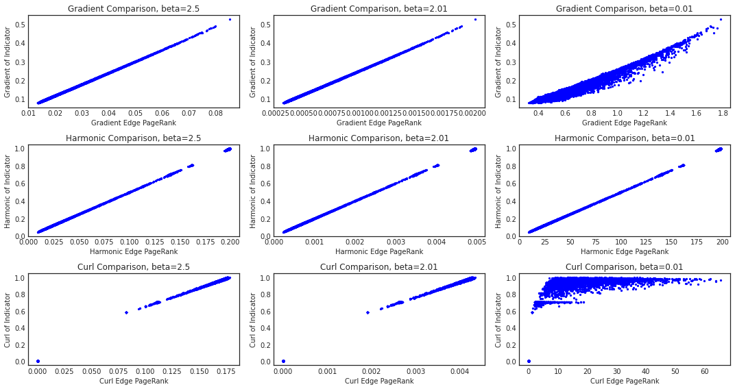
Figure B.1: Comparison of $2$-norm of Personalized Edge PageRank components to the $2$-norm of the Hodge Decomposition of the indicator on each edge, for all three components and different values of the $\beta$ parameter. Unless $\beta$ is taken to be small, the components tend to coincide with one another.

References

- Amburg et al. (2020) Amburg I, Veldt N, Benson AR (2020) Clustering in graphs and hypergraphs with categorical edge labels. Proceedings of the Web Conference.
- Aral (2016) Aral S (2016) The future of weak ties. American Journal of Sociology 121(6):1931–1939.
- Aral et al. (2007) Aral S, Brynjolfsson E, Van Alstyne MW (2007) Productivity effects of information diffusion in networks. Available at SSRN 987499 .
- Aral and Dhillon (2022) Aral S, Dhillon PS (2022) What (exactly) is novelty in networks? unpacking the vision advantages of brokers, bridges, and weak ties. Management Science .
- Aral and Van Alstyne (2011) Aral S, Van Alstyne M (2011) The diversity-bandwidth trade-off. American journal of sociology 117(1):90–171.
- Auer et al. (2007) Auer S, Bizer C, Kobilarov G, Lehmann J, Cyganiak R, Ives Z (2007) Dbpedia: A nucleus for a web of open data. The semantic web, 722–735 (Springer).
- Banerjee et al. (2013) Banerjee A, Chandrasekhar AG, Duflo E, Jackson MO (2013) The diffusion of microfinance. Science 341(6144).
- Benson et al. (2018) Benson AR, Abebe R, Schaub MT, Jadbabaie A, Kleinberg J (2018) Simplicial closure and higher-order link prediction. Proceedings of the National Academy of Sciences 115(48):E11221–E11230.
- Burt (2000) Burt RS (2000) The network structure of social capital. Research in organizational behavior 22:345–423.
- Burt (2002) Burt RS (2002) The social capital of structural holes. The new economic sociology: Developments in an emerging field 148(90):122.
- Chung (1997) Chung FR (1997) Spectral graph theory, volume 92 (American Mathematical Soc.).
- Easley and Kleinberg (2010) Easley D, Kleinberg J (2010) Networks, crowds, and markets, volume 8 (Cambridge university press Cambridge).
- Eckmann (1944) Eckmann B (1944) Harmonische funktionen und randwertaufgaben in einem komplex. Comment. Math. Helv. 17(1):240–255.
- Friedkin and Johnsen (1990) Friedkin NE, Johnsen EC (1990) Social influence and opinions. Journal of Mathematical Sociology 15(3-4):193–206.
- Gilbert and Karahalios (2009) Gilbert E, Karahalios K (2009) Predicting tie strength with social media. Proceedings of the SIGCHI conference on human factors in computing systems, 211–220.
- Girvan and Newman (2002) Girvan M, Newman ME (2002) Community structure in social and biological networks. Proceedings of the national academy of sciences 99(12):7821–7826.
- Granovetter (1985) Granovetter M (1985) Economic action and social structure: The problem of embeddedness. American Journal of Sociology .
- Granovetter (1973) Granovetter MS (1973) The strength of weak ties. American journal of sociology 78(6):1360–1380.
- Hansen (1999) Hansen MT (1999) The search-transfer problem: The role of weak ties in sharing knowledge across organization subunits. Administrative science quarterly 44(1):82–111.
- Hatcher (2002) Hatcher A (2002) Algebraic topology. Cambridge, UK .
- Jackson (2020) Jackson MO (2020) A typology of social capital and associated network measures. Social Choice and Welfare 54(2):311–336.
- Katz (1953) Katz L (1953) A new status index derived from sociometric analysis. Psychometrika 18(1):39–43.
- Klimt and Yang (2004) Klimt B, Yang Y (2004) The enron corpus: A new dataset for email classification research. European Conference on Machine Learning, 217–226 (Springer).
- Kossinets and Watts (2006) Kossinets G, Watts DJ (2006) Empirical analysis of an evolving social network. science 311(5757):88–90.
- Krackhardt et al. (2003) Krackhardt D, Nohria N, Eccles B (2003) The strength of strong ties. Networks in the knowledge economy 82.
- Lim (2020) Lim LH (2020) Hodge laplacians on graphs. SIAM Review 62(3):685–715.
- Marsden and Campbell (1984) Marsden PV, Campbell KE (1984) Measuring tie strength. Social forces 63(2):482–501.
- Mastrandrea et al. (2015) Mastrandrea R, Fournet J, Barrat A (2015) Contact patterns in a high school: a comparison between data collected using wearable sensors, contact diaries and friendship surveys. PloS one 10(9):e0136497.
- Mattie et al. (2018) Mattie H, Engø-Monsen K, Ling R, Onnela JP (2018) Understanding tie strength in social networks using a local “bow tie” framework. Scientific reports 8(1):1–9.
- Onnela et al. (2007) Onnela JP, Saramäki J, Hyvönen J, Szabó G, Lazer D, Kaski K, Kertész J, Barabási AL (2007) Structure and tie strengths in mobile communication networks. Proceedings of the national academy of sciences 104(18):7332–7336.
- Padgett and Ansell (1993) Padgett JF, Ansell CK (1993) Robust action and the rise of the medici, 1400-1434. American journal of sociology 98(6):1259–1319.
- Page et al. (1999) Page L, Brin S, Motwani R, Winograd T (1999) The pagerank citation ranking: Bringing order to the web. Technical report, Stanford InfoLab.
- Panzarasa et al. (2009) Panzarasa P, Opsahl T, Carley KM (2009) Patterns and dynamics of users’ behavior and interaction: Network analysis of an online community. Journal of the American Society for Information Science and Technology 60(5):911–932.
- Paranjape et al. (2017) Paranjape A, Benson AR, Leskovec J (2017) Motifs in temporal networks. Proceedings of the Tenth ACM International Conference on Web Search and Data Mining, 601–610.
- Park et al. (2018) Park PS, Blumenstock JE, Macy MW (2018) The strength of long-range ties in population-scale social networks. Science 362(6421):1410–1413.
- Rajkumar et al. (2022) Rajkumar K, Saint-Jacques G, Bojinov I, Brynjolfsson E, Aral S (2022) A causal test of the strength of weak ties. Science 377(6612):1304–1310.
- Reagans and McEvily (2003) Reagans R, McEvily B (2003) Network structure and knowledge transfer: The effects of cohesion and range. Administrative science quarterly 48(2):240–267.
- Reagans and Zuckerman (2001) Reagans R, Zuckerman EW (2001) Networks, diversity, and productivity: The social capital of corporate r&d teams. Organization science 12(4):502–517.
- Sapiezynski et al. (2019) Sapiezynski P, Stopczynski A, Lassen DD, Lehmann S (2019) Interaction data from the copenhagen networks study. Scientific Data 6(1):1–10.
- Schaub et al. (2020) Schaub MT, Benson AR, Horn P, Lippner G, Jadbabaie A (2020) Random walks on simplicial complexes and the normalized hodge 1-laplacian. SIAM Review 62(2):353–391.
- Sinha et al. (2015) Sinha A, Shen Z, Song Y, Ma H, Eide D, Hsu BJ, Wang K (2015) An overview of microsoft academic service (mas) and applications. Proceedings of the 24th international conference on world wide web, 243–246.
- Smith (2005) Smith SS (2005) “don’t put my name on it”: Social capital activation and job-finding assistance among the black urban poor. American journal of sociology 111(1):1–57.
- Stehlé et al. (2011) Stehlé J, Voirin N, Barrat A, Cattuto C, Isella L, Pinton JF, Quaggiotto M, Van den Broeck W, Régis C, Lina B, et al. (2011) High-resolution measurements of face-to-face contact patterns in a primary school. PloS one 6(8):e23176.
- Uzzi and Spiro (2005) Uzzi B, Spiro J (2005) Collaboration and creativity: The small world problem. American journal of sociology 111(2):447–504.
- Wu et al. (2010) Wu Y, Zhou C, Xiao J, Kurths J, Schellnhuber HJ (2010) Evidence for a bimodal distribution in human communication. Proceedings of the national academy of sciences 107(44):18803–18808.