gammaALPs: An open-source python package for computing photon-axion-like-particle oscillations in astrophysical environments

Abstract

Axions and axion-like particles (ALPs) are hypothetical particles that occur in extensions of the Standard Model and are candidates for cold dark matter. They could be detected through their oscillations into photons in the presence of external electromagnetic fields. gammaALPs is an open-source python framework that computes the oscillation probability between photons and axions/ALPs. In addition to solving the photon-ALP equations of motion, gammaALPs includes models for magnetic fields in different astrophysical environments such as jets of active galactic nuclei, intra-cluster and intergalactic media, and the Milky Way. Users are also able to easily incorporate their own custom magnetic-field models. We review the basic functionality and features of gammaALPs, which is heavily based on other open-source scientific packages such as numpy and scipy. Although focused on gamma-ray energies, gammaALPs can be easily extended to arbitrary photon energies.

1 Introduction

Several extension of the standard model predict the existence of axions and, more generally, axion-like particles (ALPs) [see, e.g., 1, for a review]. Such particles are candidates to explain the cold dark matter content in the Universe and the axion can resolve the strong CP problem of the strong interactions. Strategies to search for these particles often utilize their predicted coupling to photons in the presence of electromagnetic fields. The coupling is described through the Lagrangian [2],

$$\mathcal{L}_{a\gamma}=-\frac{1}{4}g_{a\gamma}F_{\mu\nu}\tilde{F}^{\mu\nu}a=g_{a\gamma}\mathbf{E}\cdot\mathbf{B}a,$$ (1)

where $F_{\mu\nu}$ is the electromagnetic field tensor for electric and magnetic fields $\mathbf{E}$ and $\mathbf{B}$, respectively, $\tilde{F}_{\mu\nu}$ is its dual, $a$ is the ALP field strength, and $g_{a\gamma}$ is the photon-ALP coupling constant. Hints for the existence of ALPs from the observations of active galactic nuclei (AGNs) at $\gamma$-ray energies spurred the interest in these particles in the astroparticle physics community, however, the evidence remains debated in the literature [see, e.g., 3, for a review]. Additionally, the absence of oscillation features in $\gamma$-ray (and X-ray) spectra has been used to constrain the coupling strength between ALPs and photons [see, e.g., 4, 5, 6].

Several authors have studied the oscillations between high-energy photons and ALPs in different astrophysical magnetic field environments [e.g., 7, 8, 9, 10, 11, 12, 13, 14]. Here, we present the gammaALPs package, an open-source code written in python which calculates numerically the photon-ALP oscillation probability in various astrophysical environments. It is based on numpy [15], scipy [16], and astropy [17] and uses numba [18] to speed up calculations. In addition to various models for magnetic fields along the line of sight to astrophysical sources, it is also possible to provide user-defined models. Although originally intended for the application in high-energy $\gamma$-ray astronomy, it can in principle be used for arbitrary photon energies.

The source code of gammaALPs is hosted on GitHub and is licensed under the 3-clause BSD license. Users can contribute to the code via pull requests. Bug reports and proposals for new functionality can be made through the GitHub issue tracking system. The full online documentation is available at https://gammaalps.readthedocs.io.

2 Installation

Up-to-date installation instructions can be found in the online documentation. In a nutshell, the latest release can be installed using the pip package management tool:

⬇

1pip install gammaalps

Support for an installation through the conda package manager is foreseen in the near future. A digital object identifier for the gammaALPs is provided through zenodo.org.

3 Solving the photon-ALP equations of motion

The gammaALPs code solves the equations of motion for photon-ALP oscillations using transfer matrices. A detailed solution is provided, e.g., in Refs. [19, 8] and we provide a summary below (following [10]) where we highlight important differences and newly implemented features. The equations of motion can be derived from the effective Lagrangian,

$$\mathcal{L}=\mathcal{L}_{a\gamma}+\mathcal{L}_{\mathrm{EH}}+\mathcal{L}_{a},$$ (2)

where the second term is the effective Euler-Heisenberg Lagrangian and the ALP mass and kinetic terms are $\mathcal{L}_{a}=\frac{1}{2}\partial_{\mu}a\partial^{\mu}a-\frac{1}{2}m^{2}_{a}a^{2}$. Without the loss of generality, in gammaALPs the propagation direction is assumed to be along the $x_{3}$ direction. ALPs only couple to photons in the presence of a transversal magnetic field $\mathbf{B}_{\perp}$ [2], i.e. the $B$-field component in the $\hat{x}_{1}$-$\hat{x}_{2}$ plane. We let $\psi$ denote the angle that $\mathbf{B}_{\perp}$ forms with the ${x}_{2}$ axis. Assuming for simplicity $\psi=0$, a monochromatic photon-ALP beam with energy $E$ and photon polarisation states $A_{1}$ and $A_{2}$ propagating in a cold plasma filled with a homogeneous magnetic field obeys the equation

$$\left(i\frac{\mathrm{d}}{\mathrm{d}x_{3}}+E+\mathcal{M}_{0}\right)\Psi(x_{3})=0,$$ (3)

with $\Psi(x_{3})=(A_{1}(x_{3}),A_{2}(x_{3}),a(x_{3}))^{T}$ and the mixing matrix $\mathcal{M}_{0}$,

$$\mathcal{M}_{0}=\begin{pmatrix}\Delta_{\perp}&0&0\\ 0&\Delta_{||}&\Delta_{a\gamma}\\ 0&\Delta_{a\gamma}&\Delta_{a}\end{pmatrix},$$ (4)

where Faraday rotation has been neglected. The momentum differences $\Delta_{||,\perp}$ arise due to the effects of the propagation of photons in a plasma, QED vacuum polarisation, photon-photon dispersion in background radiation fields [20], and possible photon absorption [e.g., 8], $\Delta_{\perp}=\Delta_{\mathrm{pl}}+2\Delta_{\mathrm{QED}}+\chi-i\Gamma/2$, and $\Delta_{||}=\Delta_{\mathrm{pl}}+7/2\Delta_{\mathrm{QED}}+\chi-i\Gamma/2$. The plasma term $\Delta_{\mathrm{pl}}=-\omega_{\mathrm{pl}}/(2E)$ depends on the electron density $n_{\mathrm{e}}$ through the plasma frequency $\omega_{\mathrm{pl}}^{2}=4\pi n_{e}e^{2}/m_{e}$, with the electric charge $e$ and electron mass $m_{e}$. The QED vacuum polarisation is given by $\Delta_{\mathrm{QED}}=\alpha E/(45\pi)(B/(B_{\mathrm{cr}}))^{2}$, with the fine-structure constant $\alpha$, and the critical magnetic field $B_{\mathrm{cr}}=m^{2}_{e}/|e|\sim 4.4\times 10^{13}\,$G. The photon dispersion term $\chi$ will depend on the energy density of the relevant background radiation fields. If only the cosmic microwave background (CMB) is of importance and the photons have energies far below the threshold of electron-positron pair production, it reads $\chi=44\alpha^{2}U_{\mathrm{CMB}}/(135m_{e}^{4})E$, where $U_{\mathrm{CMB}}$ is the total CMB energy density [20]. Photon absorption through, e.g., pair production, is given by the inverse mean free path (i.e., interaction rate) $\Gamma$. The kinetic term for the ALP is $\Delta_{a}=-m_{a}^{2}/(2E)$ and photon-ALP mixing is the result of the off-diagonal elements $\Delta_{a\gamma}=g_{a\gamma}B/2$. In gammaALPs, the $\Delta$ terms are calculated in units of $\mathrm{kpc}^{-1}$ and the energy is assumed to be in GeV. The ALP mass is stored in units of neV and the photon-ALP coupling in units of $10^{-11}\,\mathrm{GeV}^{-1}$.

For an unpolarised photon beam, Eq. (3) can be written in terms of the density matrix $\rho(x_{3})=\Psi(x_{3})\Psi(x_{3})^{\dagger}$ that obeys the von-Neumann-like commutator equation $i\frac{\mathrm{d}\rho}{\mathrm{d}x_{3}}=[\rho,\mathcal{M}_{0}]$. It is solved through $\rho(x_{3})=\mathcal{T}(x_{3},0;E)\rho(0)\mathcal{T}^{\dagger}(x_{3},0;E)$, with the transfer matrix $\mathcal{T}$ that solves Eq. (3) with $\Psi(x_{3})=\mathcal{T}(x_{3},0;E)\Psi(0)$ and initial condition $\mathcal{T}(0,0;E)=1$. For the general case where $\psi\neq 0$, the solutions have to be modified with a similarity transformation and, consequently, $\mathcal{M}$ and $\mathcal{T}$ will depend on $\psi$.

Several models for different astrophysical magnetic field environments are implemented in gammaALPs (see below) and the photon-ALP beam can traverse several of these environments from a source to the observer. For each environment $m$, we make the assumption that we can split the path into $N_{m}$ consecutive domains where in each domain the magnetic field, $\psi$, electron density, and dispersion terms $\chi$ are constant. The transfer matrix of each environment $m=1,\ldots,M$, where $m=1$ denotes the environment closest to the source, is then found through matrix multiplication and the final transfer matrix from source to observer is given by

$$\mathcal{T}_{\mathrm{tot}} = \mathcal{T}_{M}(x_{3,N_{M}},x_{3,N_{M-1}};E)\cdots\mathcal{T}_{1}(x_{3,N_{1}},x_{3,0};E)$$ (5)

$$= \prod\limits_{m=1}^{M}\prod\limits_{n=1}^{N_{m}}\mathcal{T}_{M-m+1}(x_{3,N_{M-m+1}-n+1},x_{3,N_{M-m+1}-n};E).$$

In the above equation, $x_{3,0}=0$, i.e. the coordinate closest to the source that produces a beam with initial polarization $\rho(0)$. The total photon survival probability is then given by

$$P_{\gamma\gamma}=\mathrm{Tr}\left((\rho_{11}+\rho_{22})\mathcal{T}_{\mathrm{tot}}\rho(0)\mathcal{T}_{\mathrm{tot}}^{\dagger}\right),$$ (6)

with $\rho_{11}=\mathrm{diag}(1,0,0)$, $\rho_{22}=\mathrm{diag}(0,1,0)$, and $\rho(0)=\mathrm{diag}(1/2,1/2,0)$ for an initially unpolarized beam. Note that the transfer matrices adjacent to $\rho(0)$ in Eq. (6) correspond to the domain closest to the source.

4 Implemented astrophysical environments

In Table 1, we provide a list of the astrophysical environments currently implemented in gammaALPs. From source to the observer they include (i) two models at different levels of sophistication for AGN jets in which the $\gamma$-ray emission is produced; (ii) two models for magnetic fields in galaxy clusters, one with a simple cell-like structure, the other one describes the $B$ field as a field with Gaussian turbulence; (iii) a simple cell-like model for the intergalactic magnetic field (IGMF), which evolves with redshift and includes $\gamma$-ray absorption on the extragalactic background light (EBL); (iv) the Galactic magnetic field of the Milky Way, where the user can choose between three different models provided in the literature, namely the ASS and BSS models in Ref. [22], the model of Ref. [23], or an updated version of the latter provided in Ref. [24]. Additionally, an environment with pure EBL absorption and no photon-ALP mixing is provided, as well as the possibility to use externally computed $B$ fields and electron densities. Further details on the individual environments are provided in the respective references given in the table. More information can also be found in the gammaALPs online documentation and tutorials.

Environment	Description	$B$-field	$n_{\mathrm{el}}$	Ref.
Name		Model	Model
Jet	Mixing in the toroidal magnetic field	Power law in distance	Power law in distance	[10, 13]
	of an AGN jet	from central black hole	from central black hole
JetHelicalTangled	Mixing in the helical and tangled	Power law in distance	Power law in distance	[14]
	magnetic fields of an AGN jet	from central black hole	from central black hole
ICMCell	Mixing in a galaxy cluster magnetic field	Constant in each cell		[9, 25]
	with a cell-like structure decreasing	with randomly varying $\psi$	(generalized) $\beta$ profile for
	with growing distance from	decreasing as	galaxy clusters
	cluster center following $n_{\mathrm{el}}(r)$	a function in $n_{\mathrm{el}}(r)$
ICMGaussTurb	Mixing in a galaxy cluster magnetic field			[10]
	with Gaussian turbulence decreasing	Field with Gaussian	(generalized) $\beta$ profile for
	with growing distance from	turbulence decreasing as	galaxy clusters
	cluster center following $n_{\mathrm{el}}(r)$	a function in $n_{\mathrm{el}}(r)$
IGMF	Mixing in the intergalactic magnetic field	Constant in each cell	constant	[8]
	with a cell-like structure,	with randomly varying $\psi$	(evolves with redshift)
	including EBL absorption
GMF	Mixing in the coherent component of	Models of Refs. [22, 23, 24]	constant	[9]
	the magnetic field of the Milky Way
EBL	No mixing, only	–	–	–
	photon absorption on EBL
File	Environment initialized	As provided in the file	As provided in the file	–
	from file
Array	Environment initialized	As provided in the array	As provided in the array	–
	from numpy array

Table 1: Implemented environments in the gammaALPs code. References that describe the models for the magnetic fields and the electron densities are given in the last column.

5 Workflow

The python code of a typical workflow example is shown below in Listing 1, which demonstrates the basic features of the API of gammaALPs. This particular example assumes as a source NGC 1275, the central AGN of the Perseus galaxy cluster, and calculates mixing in the intra-cluster field and the Milky Way. No mixing in the IGMF is assumed and only EBL absorption is used. The same parameters as in Ref. [5] are chosen for the cluster field. After the basic imports from the gammaALPs.core module, the user defines a $\gamma$-ray source with redshift and sky coordinates. The sky coordinates are necessary for $B$-field environments that depend on the sky position such as the Galactic magnetic field. Next, the user initializes the ALP class, which stores the ALP mass and coupling to be used throughout the calculation. After setting the desired energy range and initial polarization matrix $\rho(0)$, the user then initializes the ModuleList class which stores the different astrophysical environments. An environment is added with the add_propagation function which takes the name of the environment (as listed in Table 1), the positional index with respect to the source as inputs, and environment specific model parameters. The positional index 0 corresponds to the environment closest to the source. After the user has specified all desired environments, the conversion probability into the final polarization states is calculated by calling the run function.

⬇

1from gammaALPs.core import Source, ALP, ModuleList

2import numpy as np

3

4# define the source

5ngc1275 = Source(z=0.017559, ra=’03h19m48.1s’, dec=’+41d30m42s’)

6

7# define the ALP with mass in neV and coupling in 1e-11 GeV^-1

8m, g = 1.,1.

9alp = ALP(m,g)

10

11# define an energy range in GeV

12EGeV = np.logspace(1., 3.5, 250)

13

14# define the initial polarization

15pin = np.diag((1.,1.,0.)) * 0.5

16

17# initialize the module list

18ml = ModuleList(alp, ngc1275, pin=pin, EGeV=EGeV)

19# add propagation modules

20# first, mixing in Gaussian turbulent field

21ml.add_propagation("ICMGaussTurb",

22 0, # position of module counted from the source.

23 nsim=10, # number of random B-field realizations

24 B0=10., # rms of B field in muG

25 # parameters for electron density,

26 # see Churazov et al. 2003, Eq. 4

27 n0=3.9e-2,

28 n2=4.05e-3,

29 r_core=80.,

30 r_core2=280.,

31 beta=1.2,

32 beta2=0.58,

33 r_abell=500., # extension of the cluster in kpc

34 eta=0.5, # scaling of B-field with electron density

35 kL=0.18, # maximum turbulence scale in kpc^-1

36 kH=9., # minimum turbulence scale

37 q=-2.80, # turbulence spectral index

38 seed=0 # random seed for reproducability

39 )

40# EBL attenuation comes second, after beam has left cluster

41ml.add_propagation("EBL",1, eblmodel=’dominguez’)

42# finally, the beam enters the Milky Way Field

43ml.add_propagation("GMF",2, model=’jansson12’)

44

45# calculate the final polarization states

46# for photon polarization along x and y

47# and ALP polarization state

48px, py, pa = ml.run()

49

50# the total photon survival probability is

51# the sum of the final photon states

52pgg = px + py

Listing 1: Python code example of the gammaALPs workflow.

Before calling run, the user can also change the ALP parameters for which the mixing is calculated. For example, an ALP mass of 30 neV and coupling of $g_{a\gamma}=5\times 10^{-12}\,\mathrm{GeV}^{-1}$ is set by ml.alp.m = 30.; ml.alp.g = 0.5. Furthermore, run supports multiprocessing (using python’s built-in multiprocessing package). The actual calculation of the transfer matrices is sped up by using numba [18]. We show the assumed magnetic field and the electron density as well as the final $P_{\gamma\gamma}$ in Figure 1. On a MacBook Pro with a 2.7 GHz Intel Core i7 and 16GB RAM the calculation of $P_{\gamma\gamma}$ for this example (in total 4600 magnetic domains, 10 random realizations, 250 steps in energy) took $(17.7\pm 0.5)\,\mathrm{s}$.

It is also worth mentioning that each environment can take a two-dimensional spline interpolation function as a keyword chi for the photon-photon dispersion. For example, for the Galactic magnetic field, this could be an interpolated function for $\chi$ in terms of energy and distance traveled along the line of sight in the Milky Way, which describes the dispersion in the intestellar radiation fields (this was used, e.g., in Ref. [26]). Further examples for other environments are provided in the gammaALPs tutorials.

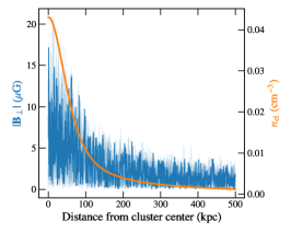
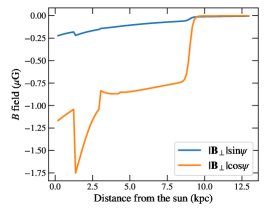
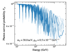
Figure 1: Example of gammaALPs environment models and final output. Left: 10 random realizations of the intra-cluster magnetic field as a function of the distance to the cluster center. The absolute value of the transversal magnetic field is shown with one realization highlighted as a solid blue line. The electron density is shown in orange (right $y$-axis). Center: The transversal components of the Galactic magnetic field towards NGC 1275 is shown as a function of the distance from the sun. Right: Resulting final photon survival probabilities for the 10 random $B$-field realizations. The same realization as in the left panel is highlighted with a solid blue line.

6 Conclusions

We have presented the open-source gammaALPs python package, which computes photon-ALP oscillations in various astrophysical environments. The code features several models for astrophysical magnetic fields and electron distributions but it is also possible to provide custom $B$-field and electron density models. As illustrated in these proceedings, with only a few lines of code it is possible to set up the models and run the calculation of the photon-ALP oscillation probability.

Beyond the calculation of the photon-ALP conversion probability, the code can also be used for other astrophysical applications. For example, the python implementations of the Galactic field models can be useful for cosmic-ray propagation studies. It is also possible to calculate the rotation measure from the Gaussian turbulent magnetic field.

In terms of future developments, it would be interesting to implement further models for astrophysical environments, such as a more realistic model for the IGMF, or dedicated models for the magnetic fields around magnetic white dwarfs and neutron stars. Also, further gains in terms of speed might be achieved through the efficient use of GPU programming.

References

- [1] I. G. Irastorza and J. Redondo, Progress in Particle and Nuclear Physics 102 (2018) 89–159, [1801.08127].
- [2] G. Raffelt and L. Stodolsky, Phys. Rev. D 37 (1988) 1237–1249.
- [3] M. Meyer, arXiv e-prints (2016) arXiv:1611.07784, [1611.07784].
- [4] A. Abramowski, F. Acero, F. Aharonian et al., Phys. Rev. D 88 (2013) 102003, [1311.3148].
- [5] M. Ajello, A. Albert, B. Anderson et al., Phys. Rev. Lett. 116 (2016) 161101, [1603.06978].
- [6] C. S. Reynolds, M. C. D. Marsh, H. R. Russell et al., ApJ 890 (2020) 59, [1907.05475].
- [7] C. Csáki, N. Kaloper, M. Peloso et al., J. Cosmology Astropart. Phys 2003 (2003) 005, [hep-ph/0302030].
- [8] A. de Angelis, G. Galanti and M. Roncadelli, Phys. Rev. D 84 (2011) 105030, [1106.1132].
- [9] D. Horns, L. Maccione, M. Meyer et al., Phys. Rev. D 86 (2012) 075024, [1207.0776].
- [10] M. Meyer, D. Montanino and J. Conrad, J. Cosmology Astropart. Phys 2014 (2014) 003, [1406.5972].
- [11] M. Simet, D. Hooper and P. D. Serpico, Phys. Rev. D 77 (2008) 063001, [0712.2825].
- [12] K. A. Hochmuth and G. Sigl, Phys. Rev. D 76 (2007) 123011, [0708.1144].
- [13] F. Tavecchio, M. Roncadelli and G. Galanti, Physics Letters B 744 (2015) 375–379, [1406.2303].
- [14] J. Davies, M. Meyer and G. Cotter, Phys. Rev. D 103 (2021) 023008, [2011.08123].
- [15] C. R. Harris, K. J. Millman, S. J. van der Walt et al., Nature 585 (2020) 357–362.
- [16] P. Virtanen, R. Gommers, T. E. Oliphant et al., Nature Methods 17 (2020) 261–272.
- [17] Astropy Collaboration, T. P. Robitaille, E. J. Tollerud et al., A&A 558 (2013) A33, [1307.6212].
- [18] S. K. Lam, A. Pitrou and S. Seibert, in Proceedings of the Second Workshop on the LLVM Compiler Infrastructure in HPC - LLVM '15, ACM Press, 2015, DOI.
- [19] N. Bassan, A. Mirizzi and M. Roncadelli, J. Cosmology Astropart. Phys 2010 (2010) 010, [1001.5267].
- [20] A. Dobrynina, A. Kartavtsev and G. Raffelt, Phys. Rev. D 91 (2015) 083003, [1412.4777].
- [21] R. Perna, W. C. G. Ho, L. Verde et al., ApJ 748 (2012) 116, [1201.5390].
- [22] M. S. Pshirkov, P. G. Tinyakov, P. P. Kronberg et al., ApJ 738 (2011) 192, [1103.0814].
- [23] R. Jansson and G. R. Farrar, ApJ 757 (2012) 14, [1204.3662].
- [24] Planck Collaboration, R. Adam, P. A. R. Ade et al., A&A 596 (2016) A103, [1601.00546].
- [25] M. Meyer, D. Horns and M. Raue, Phys. Rev. D 87 (2013) 035027, [1302.1208].
- [26] H. Vogel, R. Laha and M. Meyer, arXiv e-prints (2017) arXiv:1712.01839, [1712.01839].