Integrable spin chains and cellular automata with medium range interaction

Abstract

We study integrable spin chains and quantum and classical cellular automata with interaction range $\ell\geq 3$. This is a family of integrable models for which there was no general theory so far. We develop an algebraic framework for such models, generalizing known methods from nearest neighbor interacting chains. This leads to a new integrability condition for medium range Hamiltonians, which can be used to classify such models. A partial classification is performed in specific cases, including $U(1)$-symmetric three site interacting models, and Hamiltonians that are relevant for interaction-round-a-face models. We find a number of models which appear to be new. As an application we consider quantum brickwork circuits of various types, including those that can accommodate the classical elementary cellular automata on light cone lattices. In this family we find that the so-called Rule150 and Rule105 models are Yang-Baxter integrable with three site interactions. We present integrable quantum deformations of these models, and derive a set of local conserved charges for them. For the famous Rule54 model we find that it does not belong to the family of integrable three site models, but we can not exclude Yang-Baxter integrability with longer interaction ranges.

I Introduction

One dimensional quantum integrable models are special many body systems, which allow for exact solutions of their dynamics. Their study goes back to the solutions of the Heisenberg spin chain by H. Bethe in 1931 [1] and the exact treatment of the 2D classical Ising model by L. Onsager in 1944 [2]. It was understood in the 60’s and 70’s that a key element appearing in various types of quantum integrable models is the Yang-Baxter equation, independently discovered by C. N. Yang [3] and R. Baxter [4]. A common algebraic framework was afterwards developed by the L. Faddeev and the Leningrad group (see for example the historical review [5]). These elements of integrability connect seemingly different types of models, such as the 2D integrable statistical physical models (for example the six vertex and eight vertex models), the famous integrable spin chains such as the Heisenberg model or the Hubbard model, non-relativistic quantum gas models [6], and integrable Quantum Field Theories (iQFT) [7].

A re-occurring question over the decades has been the classification of (quantum) integrable models, together with an attempt to give a precise definition of what integrability actually is. It appears that there is no single definition encompassing all possible integrable models, but there are two very common elements appearing in integrable models: the existence of a large set of extra conservation laws, and a completely elastic and factorized scattering of the physical excitations [8]. Then the attempts for the classification can proceed along the lines of either the charges [8], or by finding all possible factorized $S$-matrices as in iQFT [7].

Focusing on quantum spin chains two big families of models have been studied extensively: those with nearest neighbor (n.n.) interactions, and some long range models. In the latter case spins at an arbitrary distance can interact, although with strongly decreasing coupling constants. The n.n. chains can be treated with the algebraic methods developed by the Leningrad group [9], which are routinely used today. On the other hand, the treatment of the long range chains is typically more involved. Examples are the Haldane-Shastry chain [10, 11] or the Inozemtsev chain [12] or long range version of the Hubbard model [13]. In such cases the construction of the exact eigenstates and also the charges is typically more complicated than in the n.n. chains, see for example [14, 15, 16].

Returning to the nearest neighbor chains, partial classifications have been achieved in certain specific cases. Integrable nearest neighbor Hamiltonians are intimately connected with so-called regular solutions of the Yang-Baxter (YB) equation. Thus a classification can proceed by finding all solutions of the YB equation; this is possible within restricted parameter spaces. For example it was understood very early that solutions can be found by assuming underlying group or quantum group symmetries [17, 18, 19, 20, 21]. However, the (quantum) group symmetric cases do not exhaust all possibilities, and it is also desirable to find the remaining models. It is not possible to list here all known integrable n.n. chains, therefore we just mention a few works that performed classifications with certain restrictions [22, 23, 24, 25, 26, 27]. More recently a systematic method was worked out in [28, 29, 30, 31, 32], based on well established ideas [33] but leading to more detailed classifications than in prior works.

Despite all of this progress there is a class of models which has so far received relatively little attention: Translationally invariant spin chains where the Hamiltonian has a finite interaction range $\ell\geq 3$. We call these models “medium range spin chains” to distinguish them both from the nearest neighbor and the long range cases. It is important that we are interested in models where the finite range Hamiltonian is the smallest dynamical charge, so we dismiss those cases when the Hamiltonian is chosen as a linear combination of some of the short range charges of a n.n. interacting chain. These cases can be interesting on their own right (see for example [34]), but we are looking for models with genuinely new interactions. We also exclude those models, where the Hilbert space is a constrained subspace of the usual tensor product space of the spin chains; an important example is the constrained XXZ model and its generalizations treated for example in [35, 36, 37, 38, 39, 40, 41] or the supersymmetric spin chains studied in [42, 43]. Such constraints are non-local, and we are looking for strictly local models with the usual tensor product Hilbert space.

There are various reasons why the medium range models can be interesting. First of all there is the obvious academic interest: If one was to uncover all possible integrable spin chains, then clearly one should consider these models as well. We can expect that as we increase the interaction range, more and more possibilities open up, and a full classification becomes less and less feasible in practice. Nevertheless it is desirable to develop a general theory for such models, and at least some key ideas for the classification, which can be applied in restricted parameter spaces. As a second motivation we can mention various recent research directions where medium range models were encountered.

I.1 Medium range spin chains in the literature

An early example for an interacting medium range spin chain is the Bariev-model, which has a three site Hamiltonian [44]. Generally the three site models can be pictured as a zig-zag spin ladders, and this was also used in the presentation of the Bariev model. In this work we stick to the translationally invariant representations. The algebraic explanation of the integrability of the Bariev model was given in [45, 46].

Recently there was interest in medium range chains which can be solved by free fermions of parafermions. A specific three-site model was found in [47] with generalizations studied later in [48, 49, 50]. In these models the fermions are “in disguise”, which means they are not obtained by the usual Jordan-Wigner transformation. A more general theory for such models was initiated in [51].

A specific medium range model called the “folded XXZ model” was investigated in the recent works [52, 53, 54, 55]. There are two formulations of the model, and the dynamical Hamiltonian is a four-site or three-site operator, depending on the formulation used. In the three-site formulation the model is seen as a special point of the Bariev model. It was shown in [54] that the model exhibits Hilbert space fragmentation, and it can be considered as a hard rod deformation of the XX model. Furthermore, its real time dynamics can be solved exactly in certain special quench problems, thus the model can be considered as one of the simplest interacting spin chains. It is remarkable that a spin chain with four site interactions has a simpler solution than the famous XXZ chains. This shows that it is worthwhile to explore the medium range chains.

In the recent work [56] a family of unitary transformations was studied which can generate a medium range chain starting from a nearest neighbor model. The techniques applied here originate in quantum information theory, and the transformations are members of the discrete Clifford group.

I.2 Integrable quantum circuits

We should also mention the recent interest in integrable quantum circuits and classical cellular automata. This is a topic closely connected to integrable Hamiltonians, and some of the models in the literature have medium range interactions.

The interest in quantum gate models is motivated in part by experimental advances, but also by surprising theoretical results. For example it was found that simple (non-integrable) models with random unitary gates can lead to exact solutions, see for example [57, 58, 59, 60, 61, 62, 63]. In the integrable setting there is interest for quantum circuits with unitary gates that span two, three of four sites (in the following we will often use the short term “unitary” instead of “unitary gate”).

First of all, a quantum circuit model with two-site unitaries was developed in [64]: the model serves as an integrable Trotterization (discrete time analog) of the XXZ spin chain. This idea goes back to the light cone regularization of integrable QFT’s [65, 66, 67]. More recently the same idea was also applied to dissipative systems [68]. The key observation in these works is that the so-called $R$-matrix itself can be used as a two-site quantum gate, and in certain cases this leads to discrete unitary time evolution with well defined integrability properties. The original integrable spin chains can be recovered in the continuous time limit of the quantum gate models.

An important family of quantum circuits falls outside the realm of nearest neighbor models. These are the elementary cellular automata on light cone lattices classified in [69], which can be considered quantum circuits with special three site unitaries. The most important example is the Rule54 model, which is often called the simplest interacting integrable model [70]. It is a very special model with soliton-like behaviour, which allows for exact solutions [71, 72, 73] and integrable quantum deformations [74] (see also [75]). However, the connection with the standard Yang-Baxter integrability remained unknown.

Very recently a new algebraic framework was proposed for these cellular automata [76], by making connection to the so-called Interaction Round-a-Face (IRF) models of statistical physics (see for example [77, 78, 79, 80]). In [76] new transfer matrices were developed for the classical cellular automata and certain quantum deformations of them, and it was conjectured that the new construction gives new quasi-local conserved charges in these models, thus proving their integrability. These IRF models are such that the three site quantum gates have two control bits on the two sides and one action bit in the middle. If these IRF models are indeed integrable, then they could serve as integrable Trotterization of some spin chains with three site Hamiltonians, likely having a very similar structure. However, such connections have not yet been found.

In the recent work [81] a cellular automaton was found with a four site update rule, such that it can be considered as an integrable Trotterization of the folded XXZ model mentioned above. However, the construction in [81] had some drawbacks: it did not have space reflection symmetry, and the integrability was only proven for a certain diagonal-to-diagonal transfer matrix, which is not adequate to treat the Cauchy problem. Nevertheless the results of [81] indicate that the cellular automata and medium range spin chains are indeed closely related, and can be treated with the usual algebraic methods of integrability.

We should also note that there exists a family of classical cellular automata, where the integrability properties are well understood: these are the so-called box ball systems [82, 83]. Here the update rules are non-local in the sense that they can not be formulated using a simultaneous action of local update rules; instead, they belong to the class of the so-called filter automata [84, 85, 86, 87]. The box-ball models are noteworthy, because they display solitonic behaviour, and they are connected to a number of question in representation theory of quantum groups, combinatorics, and classical integrability [83]. Recently the hydrodynamic behaviour of these models was also studied in [88]. In our paper we do not treat these models, because we are interested in strictly local systems.

I.3 The goals of this paper

Motivated by the findings discussed above, in this paper we strive towards a general theory for medium range integrable models. It is our goal to develop the common algebraic structures, which will be generalizations of the known methods applied for nearest neighbor models. We stress that up to now there has been no general framework for the medium range models, and even in those cases where the algebraic background was developed (see for example the Bariev model [45, 46]), it was based on ad hoc ideas lacking a general understanding. In contrast, in this work we establish the key relations for the medium range models, focusing in particular on the three site and four site interacting cases. A special emphasis will be put on the IRF models treated in [76]: we show that they can be embedded into our framework, and we disprove some of the conjectures made in [76]. In particular, we argue that the Rule54 model is not in the family of the three site interacting Yang-Baxter integrable models, but we do not exclude integrability with longer interaction ranges.

In Section II we set the stage for our computations: we introduce the main concepts and also explain and summarize some of our key results. The algebraic structures of integrability are then introduced in Section III, which also includes our main results about the medium range spin chains. Integrable quantum circuits of various types are constructed in Section IV. The special class of models related to the elementary cellular automata are considered in Section V. Here we also treat the results of [76]. In Section VI we study the four site interacting models. Open questions are discussed in VII, and we present some of the technical computations in the Appendices.

II Preliminaries

In this Section we introduce the key concepts regarding integrable spin chains, and we summarize our new results for the medium range cases. We also introduce the quantum circuits, which can be considered as the discrete time versions of the spin chain models. In this Section we avoid the algebraic treatment of the integrability properties, instead we focus on the overall physical properties of these models, most importantly on the set of conserved charges.

First we introduce some notations that we use throughout the work, and afterwards we discuss the spin chains and the quantum circuit models. The algebraic structures behind the integrability are presented later in Sections III and IV.

II.1 Notations

We consider homogeneous spin chains with translationally invariant Hamiltonians. The local Hilbert spaces are $V_{j}=\mathbb{C}^{d}$ with some fixed $d\geq 2$. The full Hilbert space of the model in finite volume $L$ is $\mathcal{H}=\otimes_{j=1}^{L}V_{j}$. The majority of our abstract results will not depend on the actual value of the local dimension $d$, but in the concrete examples we consider $d=2$.

We say that an operator $\mathcal{O}(j)$ is local if its support is restricted to a limited number of sites starting from $j$, such that the support does not grow with $L$ as we consider longer and longer chains. We use notation $|\mathcal{O}(j)|$ for the range of the local operator (which we also call length). This means that the support of $\mathcal{O}(j)$ with $|\mathcal{O}(j)|=\ell$ is the segment $[j,\dots,j+\ell-1]$.

If a local operator has a fixed small range $\ell$, we will also use an alternative notation where we spell out the sites on which it acts. For example for two-site operators we also write $\mathcal{O}_{j,j+1}$, for three site operators $\mathcal{O}_{j,j+1,j+2}$, and so on. We will switch between the two notations depending on which is more convenient for the actual computation.

In our concrete examples we will treat spin-1/2 chains. In these cases we use the standard basis of the up and down spins, but we will use the notations ${\left|\circ\right\rangle}={\left|0\right\rangle}$ (empty site) and ${\left|\bullet\right\rangle}={\left|1\right\rangle}$ (occupied site) for these basis states, respectively. We use the standard Pauli matrices $\sigma^{x,y,z}$ and also the standard ladder operators $\sigma^{\pm}$, together with the following projectors onto the basis states:

$$P^{\circ}=P^{0}=\frac{1+\sigma^{z}}{2},\qquad P^{\bullet}=P^{1}=\frac{1-\sigma^{z}}{2}.$$ (II.1)

An important operator that we will use often is the cyclic shift operator $\mathcal{U}$ that translates the finite chain of length $L$ to the right by one site.

II.2 Integrable spin chains with nearest neighbor interactions

In the literature there is no single definition for quantum integrability. However, it is generally accepted that one of the key properties of integrable models is the existence of a large set of additional conserved charges, which commute with each other. Then the integrable models can be classified according to the patterns of how these charges appear in the model [8].

In this paper we focus on local spin chains, where the Hamiltonian is given by a strictly local Hamiltonian density:

$$H=\sum_{j}h(j).$$ (II.2)

Here $h(j)$ is a local operator with some range $\ell$. Periodic boundary conditions are understood throughout this work.

The additional conserved charges are a set of operators $Q_{\alpha}$, where $\alpha$ is a label which we discuss below. We require that each charge should be extensive with a local density:

$$Q_{\alpha}=\sum_{j}q_{\alpha}(j).$$ (II.3)

In this work we restrict ourselves to these strictly local charges, even though it is known that in certain cases so-called quasi-local charges also play an important role [89, 90]. Furthermore, there are integrable models where the charges typically grow super-extensively with the volume, see for example the discussion of the Haldane-Shastry chain in [8]. Nevertheless, in this work we focus only on the extensive cases.

It is generally required that the conserved charges commute

$$[Q_{\alpha},Q_{\beta}]=0,$$ (II.4)

and the Hamiltonian should be a member of the set. The commutativity has to hold in every volume $L$ large enough so that both charges fit into the system.

If these requirements are met, then generally the label $\alpha$ can be chosen simply as the length of the charge density, therefore we will use the convention throughout this work

$$|q_{\alpha}(j)|=\alpha.$$ (II.5)

Within this class of models the most studied ones are nearest neighbor interacting ones, thus we can identify $H=Q_{2}$. In such cases the allowed values for $\alpha$ are the integers starting from 2. If there is also a global $U(1)$-symmetry then $\alpha=1$ is also allowed.

Within this class the most important cases are the spin-1/2 chains, for which a full classification (including non-Hermitian cases) was performed in [28, 29]. We do not treat the classification here, instead we just mention the most important examples.

Let us start with a generic (non-integrable) spin-1/2 chain and let us require space reflection invariance. Then it can be shown that the most general nearest neighbor Hamiltonian (apart from global $SU(2)$ rotations) is the XYZ model with magnetic fields:

$$H=\sum_{j}\left(J_{x}\sigma^{x}_{j}\sigma^{x}_{j+1}+J_{y}\sigma^{y}_{j}\sigma^{y}_{j+1}+J_{z}\sigma^{z}_{j}\sigma^{z}_{j+1}\right.+\\ +\left.h_{x}\sigma^{x}_{j}+h_{y}\sigma^{y}_{j}+h_{z}\sigma^{z}_{j}\right).$$ (II.6)

This model is not integrable except for special cases [91].

One integrable family is when $h_{x}=h_{y}=h_{z}=0$, and the couplings $J_{x,y,z}$ are arbitrary, this is known as the XYZ model. A special point with $U(1)$ symmetry is the XXZ chain with $J_{x}=J_{y}$, which allows for a non-zero $h_{z}$. A further special point is the $SU(2)$ invariant Heisenberg spin chain with equal couplings, which allows for arbitrary magnetic fields.

An other special integrable family within (II.6) are the so-called XYh models, where $J_{z}=0$ and $h_{x}=h_{y}=0$. A special model of this family is the quantum Ising chain where also $J_{y}=0$. The XYh family can be solved by free fermion techniques [92].

II.3 The Reshetikhin condition

A common property of the nearest neighbor models is that they satisfy the so-called Reshetikhin condition of integrability. There are multiple formulations of this condition, and now we review the most general one. The algebraic background is treated later in Section III.

First of all we quote a Conjecture that was presented in [33]. We put this in a slightly modified form:

Conjecture 1.

A nearest neighbor spin chain with a dynamical Hamiltonian $H$ is integrable iff there exists an extensive 3-site charge $Q_{3}$ which is functionally independent from $H$ and the possible one site charges of the model, and which commutes with $H$ for every volume $L\geq 3$.

As far as we know no counter-examples have been found so far, but the Conjecture has not yet been proven either. It is important that we added the condition that the Hamiltonian should be dynamical: If this condition is not satisfied, then simple counter examples can be found, see the discussion in Appendix A.

Now we also present the Reshetikhin condition in a rather general form:

Conjecture 2.

If there exists a conserved charge $Q_{3}$ commuting with the dynamical two-site Hamiltonian $H=\sum_{j}h(j)$, then it can be written as $Q_{3}=\sum_{j}q_{3}(j)$ with

$$q_{3}(j)=[h(j),h(j+1)]+\tilde{h}(j),$$ (II.7)

where $\tilde{h}(j)$ is also a two-site operator.

It might appear that the Conjecture allows for a lot of freedom due to the presence of $\tilde{h}(j)$, but the fact that this operator has to be a two-site operator is rather restrictive.

The conjecture can be proven backwards: If the spin chain is Yang-Baxter integrable, then the precise form of the density $q_{3}(j)$ follows from the underlying algebraic objects, and it has precisely the form (II.7). However, it is not known how to prove the Conjecture without assuming Yang-Baxter integrability. We put forward that $\tilde{h}(j)=0$ in models where the so-called $R$-matrix is of difference form; this corresponds to the original Reshetikhin condition treated in [33]. On the other hand, $\tilde{h}(j)\neq 0$ in other models such as the Hubbard model [93].

Conjecture 2 was used in the recent works [28, 29, 30, 31, 32] for the classification of integrable nearest neighbor chains in various circumstances. We will not review this classification here, instead we will focus on the generalization of the Reshetikhin condition to medium range spin chains.

II.4 Medium range spin chains

In this work we treat integrable spin chains and closely related quantum gate models where the interaction range is $\ell\geq 3$. We call these models “medium range chains”. We propose the following definition:

Definition 1.

A medium range integrable spin chain is a model which has an infinite set of commuting local charges $\{Q_{\alpha}\}$ where $\alpha\in\mathcal{S}$ with $\mathcal{S}\subset\mathbb{Z}^{+}$, such that the lowest dynamical charge (which is regarded as the Hamiltonian) has a range $\ell\geq 3$.

Once again it is important to add the requirement of having a dynamical charge as the Hamiltonian. A good example for the usefulness of this requirement is the so-called “folded XXZ model” treated in [52, 53, 54], where the first four charges are

$$\begin{split}Q_{1}&=\sum_{j=1}^{L}\sigma^{z}_{j},\qquad Q_{2}=\sum_{j=1}^{L}\sigma^{z}_{j}\sigma^{z}_{j+1},\\ Q_{3}&=\sum_{j}i(\sigma^{z}_{j}+\sigma^{z}_{j+3})(\sigma^{+}_{j+1}\sigma^{-}_{j+2}-\sigma^{-}_{j+1}\sigma^{+}_{j+2}),\\ Q_{4}&=\sum_{j=1}^{L}(1+\sigma^{z}_{j}\sigma^{z}_{j+3})(\sigma^{+}_{j+1}\sigma^{-}_{j+2}+\sigma^{-}_{j+1}\sigma^{+}_{j+2}).\end{split}$$ (II.8)

Based on the existence of the charge $Q_{2}$ one could regard this model as nearest neighbor interacting, but $Q_{2}$ does not generate dynamics. Instead, in this model $Q_{4}$ is regarded as the Hamiltonian, because $Q_{4}$ is the first parity symmetric dynamical charge of the model.

II.5 Three site models – general remarks

Figure 1: Graphical illustration of a zigzag spin ladder. It is natural to expect three site interactions for each plaquet.

Let us focus on the case with $\ell=3$. In this case we identify $H=Q_{3}$ and we also write

$$H=\sum_{j}h_{j,j+1,j+2},$$ (II.9)

where $h_{j,j+1,j+2}$ is the three site Hamiltonian density.

Such models can be interpreted very naturally as a zig-zag spin ladder. See figure 1. However, we will focus on the translationally invariant representation (II.9).

Our main results are finding the general algebraic structures behind the three site models, which lead to a generalization of the Reshetikhin condition. We formulate the following conjecture:

Conjecture 3.

A three site Hamiltonian is integrable, iff the charge $Q_{5}=\sum_{j}q_{5}(j)$ defined by

$$q_{5}(j)=[h_{j,j+1,j+2},h_{j+1,j+2,j+3}+h_{j+2,j+3,j+4}]+\\ +\tilde{h}_{j,j+1,j+2}$$ (II.10)

commutes with the Hamiltonian in every volume $L\geq 5$. Here $\tilde{h}_{j,j+1,j+2}$ is an other three-site operator.

Clearly, this is a generalization of Conjecture 2. The construction of $Q_{5}$ through (II.10) is one of our key results. Its derivation from an underlying algebraic theory is presented in Section III.3. We stress again that this result is very restrictive: it uses two three-site operators $h_{j,j+1,j+2}$ and $\tilde{h}_{j,j+1,j+2}$ to generate a five site charge.

Based on this result it is possible to perform a classification of integrable spin chains with 3-site interactions. This is rather analogous to the ideas used in [20, 21] and later in [28, 29, 30, 31, 32]. The idea is to make an Ansatz for $h_{j,j+1,j+2}$ and $\tilde{h}_{j,j+1,j+2}$, possibly including a number of free parameters, to construct $Q_{5}$ using (II.10) and to check the commutation relation $[H,Q_{5}]=0$ on spin chains with medium length. We implemented this strategy using the program Mathematica and performed partial classifications on spin 1/2 chains. The generic density $h_{j,j+1,j+2}$ has a total number of $8^{2}=64$ parameters, which is a too large parameter space for practical computations. Therefore we performed partial classifications along restricted subspaces which can bear physical relevance. The results are presented in Subsections III.4 and V.2.

II.6 Quantum gates and cellular automata

We also consider brickwork type quantum circuits, where the fundamental local unitaries have a support of $\ell$ sites. The interest in such models is manifold: On the one hand, they can be understood as integrable models in discrete time, or alternatively as integrable Trotterizations of the continuous time spin chain models. On the other hand, they are interesting because they can lead to classical cellular automata, thus presenting one more link between the worlds of quantum and classical integrability. Finally, they are also relevant to quantum computing and real world experiments.

Let us sketch the general schemes behind our quantum circuit models. First we present the abstract formulation of the update rules, and we give more concrete examples later. It is necessary to start with the most general form, because later in this work we consider multiple types of constructions.

We build systems with Floquet-type discrete time evolution, such that the equal time update rules are given by local unitaries. Let us fix an interaction range $\ell$, and consider a local unitary $U^{(\ell)}(j)$ which acts on the segment $[j,\dots,j+\ell-1]$ of the spin chain. Typically these unitaries will also depend on a continuous parameter $u$ (the spectral parameter) and on a small number of extra parameters characterizing a family of models. Then we construct a brickwork type update rule for the whole spin chain using the single unitaries. We build a Floquet-type cycle with time period $\tau$:

$$\mathcal{V}=\mathcal{V}_{\tau}\dots\mathcal{V}_{1},$$ (II.11)

such that each update step $\mathcal{V}_{j}$ with $j=1\dots\tau$ is a product of commuting local unitaries acting at the same time. We formalize it as

$$\mathcal{V}_{l}=\prod_{k}U^{(\ell)}(x_{k}+\Delta_{l}).$$ (II.12)

Here $x_{k}$ are coordinates that specify the placement of the local unitaries within a single time update, and $\Delta_{l}$ is a displacement which depends on the discrete time index $l$, signaling the position within the Floquet-type cycle.

The local unitaries within a given time step should commute with each other, such that the order of the product (II.12) does not matter. This requirement can be important for practical purposes (implementation of the quantum circuits in experiments), but also for theoretical reasons. In the most general case the commutativity holds if the supports are non-overlapping, i.e. $x_{k+1}\geq x_{k}+\ell$. Nevertheless the supports can have a non-zero overlap, if the commutativity is guaranteed by other means, for example if the local unitaries act diagonally on the overlapping sites.

The simplest example for the brickwork construction discussed above is the alternating circuit discussed for example in [64]. In this case $\tau=2$, we can choose $x_{k}=2k$, and $\Delta_{l}=l$ with $l=1,2$. For a graphical representation see Figure 8 later in Section IV. We can build similar structures with interaction range $\ell=3$, the most obvious choice is $\tau=3$, $x_{k}=3k$, and $\Delta_{l}=l$ with $l=1,2,3$ (see Figure 12). Such a brickwork circuit was introduced in [81]. Later we will also present other types of constructions.

As mentioned earlier, the local unitaries typically have a spectral parameter $u$ which can be tuned freely. This means that we can build families of quantum circuits. These families can have special points with very specific physical behaviour.

For example, in the most typical case the unitaries become equal to the identity at the special point $u=0$. Furthermore, the first order expansion in $u$ gives a local Hamiltonian $h$ with interaction range $\ell$. Assuming $u\in\mathbb{R}$ this is formalized as

$$U^{(\ell)}(u|j)=1+iuh_{j,\dots,j+\ell-1}+\mathcal{O}(u^{2}).$$ (II.13)

In such a case the Floquet circle $\mathcal{V}$ can act as a Trotterization of the global Hamiltonian $H$:

$$\mathcal{V}=1+iucH+\mathcal{O}(u^{2}),$$ (II.14)

where $c$ is a real number that depends on the details of the construction, such as the Floquet period $\tau$, the coordinate differences $x_{k+1}-x_{k}$ and the displacements $\Delta_{l}$ in (II.12).

We intend to construct quantum circuits with precisely such a behaviour, so that $H$ is one of our medium range integrable Hamiltonians. Furthermore we require that the quantum circuit itself should have certain integrability properties. These depend on the particular construction, and will be discussed in detail in IV; the local unitaries will be derived from the so-called Lax operators of the medium range model.

In some models the local unitaries become deterministic for a special value $u$ of the rapidity parameter. This means that $U^{(\ell)}(j)$ simply just permutes the states in the computational basis (possibly with some phases added), without creating any linear combinations. The states of the computational basis can be considered classical, because every spin has a fixed value; if the local unitaries are deterministic then classical states are mapped to classical states during time evolution. This means that the quantum circuit can be considered a classical cellular automaton at this special point $u$. An integrable example for such model was presented recently in [81]. An other important class for such models are the Interaction-Round-A-Face models treated in [76], which lead to the elementary cellular automata on light-cone lattices. In the Subsection below we discuss these models in detail.

II.7 Elementary cellular automata on light cone lattices

These are classical 2-state models where the variables are defined on a light cone lattice, see Fig. 2. The vertical dimension is interpreted as the direction of time. Each cell is updated depending on the state of its 3 neighbors (to the South-west, South, and south-East), and the update rules are homogeneous both in space and time. Accordingly, there are $2^{2^{3}}=256$ such models, and they have been studied and classified in the seminal works [94, 69]. The nomenclature for these models follows the original proposal of Wolfram [95] (see also [69]). Recently these cellular automata attracted considerable attention due to the integrability properties of some of its members: the Rule54, Rule150 and Rule201 models (see the review [70] and also [96, 97] ).

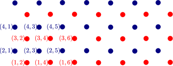
Figure 2: The light cone lattice for the elementary cellular automata. We assign coordinates $(t,x)$ to the sites, where $t$ is interpreted as a time variable. The $x$ coordinates are increased by steps of 2, and they take even (odd) values if the $t$ coordinate is odd (even), respectively. The update of the cellular automata proceeds in the time direction upwards, and each spin is given a new value using the state of 3 of its neighbors (to the directions South-West, South, and South-East). For example, the spin at position $(3,2)$ is given a value using the spins at $(2,1)$, $(1,2)$ and $(2,3)$.

As the update rules depend on 3 bits, it is tempting to look for a connection with our 3-site interacting Hamiltonians and quantum gate models. Therefore we provide here a formulation of the models which fits into the framework given above. Afterwards we provide a simple classification of the physically interesting models. Finally we summarize our main results, with the technical computation presented later in Section IV.

First we transform the light cone lattice into a regular rectangular lattice. The idea is to add new sites to the light cone lattice to the centers of the faces, see Fig. 3. Then on this rectangular lattice we formulate a Floquet-type update rule with period $\tau=2$, such that at each step the odd or even sites are updated, respectively. In this formulation the local update is performed by a three-site $U^{(3)}$ which is actually deterministic in the computational basis. Furthermore, it has a structure which was discussed already for the IRF type Hamiltonians above: The quantum gate acts diagonally on the first and last bits, whereas it has an action bit in the middle. In the particular case we have

$$U^{(3)}(j)=\sum_{a,b=0,1}P_{j}^{a}f^{ab}_{j+1}P^{b}_{j+2},$$ (II.15)

where $P^{a}_{j}$ is a projector to basis state $a$ acting on site $j$, and $f^{ab}_{j+1}$ is a collection of 4 matrices acting on site $j+1$. Then the full update rule is specified by

$$\mathcal{V}=\mathcal{V}_{2}\mathcal{V}_{1}$$ (II.16)

with

$$\mathcal{V}_{l}=\prod_{k=1}^{L/2}U^{(3)}(2k+l),\qquad l=1,2.$$ (II.17)

The neighboring three site unitaries overlap at one site, but they commute because they act diagonally on the boundary sites. Thus (II.17) is well defined without specifying the order of the action the quantum gates.

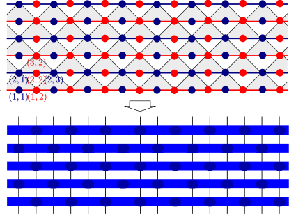
Figure 3: Two different representations for the cellular automata on the light cone lattices. – On the top we complement the original arrangement into a rectangular lattice, by adding new sites to the centers of the faces of the original lattice. The spins at the newly added sites are taken to be identical with those immediately below them, for example the state of the new site at $(2,2)$ is copied from the spin at $(1,2)$. This way we can formulate an update rule using three site unitaries on a rectangular lattice. For example the spin at $(3,2)$ is given a value using the three spins $(2,1)$, $(2,2)$ and $(2,3)$ from the previous row. The gray triangles show the direction of the update steps. – On the bottom we show a representation using quantum gates. Now the spin variables live on the vertices and three site unitaries update them. The unitary gates are placed so that the neighboring pairs overlap at a control bit, which are shown by the darker shaded circles.

Let us now discuss the classification of these models. We wish to have deterministic time evolution (without phases), and we also require time reversibility, which follows from the requirement of unitary. Therefore the only possibilities are

$$f^{ab}=1\quad\text{or}\quad f^{ab}=\sigma^{x}.$$ (II.18)

The choices (II.18) leave us with $2^{4}=16$ models. If we also require space reflection invariance we end up with $2^{3}=8$ models. Those two models where all $f^{ab}$ matrices are identical are completely trivial, which leaves us with 6 models. Out of these 6 models we can choose the following 4, which are not related to each other by overall spin reflection [76]:

$$\text{Rule54: }f^{00}=1,\quad f^{01}=f^{10}=f^{11}=\sigma^{x}$$ (II.19)

$$\text{Rule105: }f^{00}=f^{11}=\sigma^{x},\quad f^{01}=f^{10}=1$$ (II.20)

$$\text{Rule150: }f^{00}=f^{11}=1,\quad f^{01}=f^{10}=\sigma^{x}$$ (II.21)

$$\text{Rule201: }f^{00}=\sigma^{x},\quad f^{01}=f^{10}=f^{11}=1.$$ (II.22)

Additional two new models can be obtained by a complete spin reflection of the Rule54 and Rule201 models.

The Rule105 and Rule150 models are not completely independent either, because their $f$-matrices are obtained from each other by a multiplication with $\sigma^{x}$. This means that

$$\mathcal{V}_{k}^{(150)}=X_{k}\mathcal{V}_{k}^{(105)}=\mathcal{V}_{k}^{(105)}X_{k},\qquad k=1,2,$$ (II.23)

where we defined

$$X_{k}=\prod_{j=1}^{L/2}\sigma^{x}_{2j+k},\qquad k=1,2.$$ (II.24)

We can also observe the commutation relations

$$[\mathcal{V}_{1}^{(105)},X_{2}]=[\mathcal{V}_{2}^{(105)},X_{1}]=0,$$ (II.25)

and similarly for the operators of the Rule150 model. Altogether this implies that the combined Floquet steps are related as

$$\mathcal{V}^{(150)}=X\mathcal{V}^{(105)},$$ (II.26)

where $X$ is the global spin reflection operator given by

$$X=X_{2}X_{1}=\prod_{j=1}^{L}\sigma^{x}_{j}.$$ (II.27)

From these relations we can also derive

$$\left(\mathcal{V}^{(150)}\right)^{2}=\left(\mathcal{V}^{(105)}\right)^{2}.$$ (II.28)

Thus the physical behaviour of the two models could be considered the same, up to a staggered global spin reflection.

An important property of these models is that the two different possibilities for the Floquet time step are actually inverses of each other:

$$\mathcal{V}_{1}\mathcal{V}_{2}=\left(\mathcal{V}_{2}\mathcal{V}_{1}\right)^{-1}$$ (II.29)

which follows simply from

$$(\mathcal{V}_{1})^{2}=(\mathcal{V}_{2})^{2}=1.$$ (II.30)

As a result the two Floquet operators actually commute with each other:

$$[\mathcal{V}_{1}\mathcal{V}_{2},\mathcal{V}_{2}\mathcal{V}_{1}]=[\mathcal{V}_{1}\mathcal{V}_{2},\mathcal{U}^{-1}\mathcal{V}_{1}\mathcal{V}_{2}\mathcal{U}]=0.$$ (II.31)

The four models listed above have been studied in a number of works recently (see the review [70] for the Rule54 model and also [96, 97] for the Rule150 and Rule201 models), nevertheless the algebraic background for their observed integrability properties was not understood for a long time. Recently a new framework was introduced in [76] which claimed to solve this problem. We also treat these cellular automata; our main results are as follows.

We find that the Rule105 and Rule150 models can be embedded into our framework of three-site interacting models. We find a rapidity dependent family of commuting transfer matrices which includes the time evolution operator of the model as a particular case. This family of transfer matrices is regular, and we derive a set of local conserved charges that commute with the discrete time evolution operator of the cellular automata. Even though we use a different formalism, we show explicitly that our construction is identical to that one of [76] for these special class of models.

On the other hand, for the Rule54 and Rule201 we find that they are not in the family of three site interacting integrable models. In the case of the Rule54 model we also show that the transfer matrices of [76] are algebraically dependent on three known conserved charges of the model, therefore those transfer matrices do not yield new information; this is presented in Subsection V.4.

III Integrability structures

In this Section we present the integrability structures behind the spin chains under consideration. We start with a brief treatment of the nearest neighbor chains, and afterwards we turn to our new results.

III.1 Nearest neighbor interacting spin chains

We construct a transfer matrix which serves as a generating function for the conserved charges of the model under consideration. For an introduction into the methods we refer the reader to [9, 98].

First we construct the monodromy matrix as follows. We take an auxiliary space $\mathbb{C}^{d^{\prime}}$. The Lax operator $\mathcal{L}_{a,j}(u)$ acts on the tensor product of the auxiliary space (denoted by the index $a$) and a physical space with site index $j$. The variable $u$ is called spectral parameter. In those cases when the transfer matrix generates the Hamiltonian and the other charges we have $d^{\prime}=d$.

Figure 4: Graphical illustration of the operators $\check{R}_{1,2}$ and $R_{1,2}$; we suppressed the dependence on the rapidity parameters. On the left we show the usual notation which comes from the vertex models. On the right we depict the same operators as quantum gates. The two matrices differ in a permutation, and in this notation $\check{R}_{1,2}$ acts such that the two vector spaces are kept in place.

The monodromy matrix for a finite volume $L$ is defined as

$$M_{a}(u)=\mathcal{L}_{a,L}(u)\dots\mathcal{L}_{a,2}(u)\mathcal{L}_{a,1}(u),$$ (III.1)

and the transfer matrix is

$$t(u)=\text{Tr}_{a}\ M_{a}(u).$$ (III.2)

The transfer matrices form a commuting set of operators if the Lax operators satisfy the following exchange relations, where $a$ and $b$ denote two auxiliary spaces:

$$R_{b,a}(\nu,\mu)\mathcal{L}_{b,j}(\nu)\mathcal{L}_{a,j}(\mu)=\\ =\mathcal{L}_{a,j}(\mu)\mathcal{L}_{b,j}(\nu)R_{b,a}(\nu,\mu).$$ (III.3)

Here $R(u,v)$ is the so-called $R$-matrix which satisfies the Yang-Baxter relations

$$R_{12}(\lambda_{1},\lambda_{2})R_{13}(\lambda_{1},\lambda_{3})R_{23}(\lambda_{2},\lambda_{3})=\\ =R_{23}(\lambda_{2},\lambda_{3})R_{13}(\lambda_{1},\lambda_{3})R_{12}(\lambda_{1},\lambda_{2}).$$ (III.4)

The figure 4 shows the graphical presentation of the $R$-matrix. In the models of physical relevance the $R$-matrix also satisfies the so-called regularity property

$$R_{ab}(u,u)\sim\mathcal{P}_{ab},$$ (III.5)

where $\mathcal{P}_{ab}$ is the permutation operator acting on the tensor product space.

If the regularity condition holds then the following inversion can be established:

$$R_{12}(\lambda,\mu)R_{21}(\mu,\lambda)\sim 1,$$ (III.6)

where

$$R_{21}(\mu,\lambda)=\mathcal{P}R_{12}(\mu,\lambda)\mathcal{P}.$$ (III.7)

For the sake of completeness we present the derivation of (III.6) using the Yang-Baxter equations and (III.5) in Appendix C.

One can use the $R$-matrix itself as a Lax operator:

$$\mathcal{L}_{a,j}(\mu)=R_{a,j}(\mu,\xi_{0}),$$ (III.8)

where $\xi_{0}$ is a fixed parameter of the model. In such a case the YB relation is equivalent to the RLL relation and the transfer matrix reads as

$$t(u)=\mathrm{Tr}_{a}R_{a,L}(u,\xi_{0})\dots R_{a,2}(u,\xi_{0})R_{a,1}(u,\xi_{0}).$$ (III.9)

There is an alternative way to define a transfer matrix, where the ordering of the sites is the opposite, and the role of the auxiliary and physical spaces is exchanged:

$$\bar{t}(u)=\mathrm{Tr}_{a}R_{1,a}(\xi_{0},u)R_{2,a}(\xi_{0},u)\dots R_{L,a}(\xi_{0},u).$$ (III.10)

It can be proven using the Yang-Baxter relation that

$$[t(u),\bar{t}(v)]=0.$$ (III.11)

In some of our constructions below it will be more convenient to use (III.10) instead of (III.9). In figure 5 and 6 we can see the graphical presentations of these two transfer matrices.

Figure 5: Graphical illustration of transfer matrix (III.9). Here $a$ denotes the auxiliary space. The first representation is the usual from the literature, which shows the transfer matrix as a concatenation of Lax operators. The second picture shows the same object using a succession of quantum gates. The two representations are not very different, but generalizations of the second one will be more convenient in the more complicated cases that will follow.

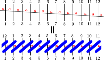
Figure 6: Graphical illustration of transfer matrix (III.10).

The regularity condition ensures that at the special point $\xi_{0}$ we have the initial conditions

$$t(\xi_{0})=\mathcal{U},\qquad\bar{t}(\xi_{0})=\mathcal{U}^{-1}$$ (III.12)

where $\mathcal{U}$ is the cyclic shift operator on the chain.

A commuting set of local charges is then constructed as

$$Q_{\alpha}\quad\sim\quad\left.(\partial_{u})^{\alpha-1}\log(t(u))\right|_{u=\xi_{0}}.$$ (III.13)

In many models the $R$-matrix is of difference form, which means

$$R(u,v)=R(u-v).$$ (III.14)

In such a case the parameter $\xi_{0}$ is irrelevant, and it is conventional to set it to $\xi_{0}=0$. However, we will consider the generic case where the $R$-matrix is not necessarily of difference form.

Let us investigate the first few charges in detail. Performing the first derivative of (III.13) we get the nearest neighbor Hamiltonian

$$H=Q_{2}=\sum h_{j,j+1}$$ (III.15)

with

$$h_{j,j+1}=\left.\partial_{u}\check{\mathcal{L}}_{j,j+1}(u)\right|_{u=\xi_{0}},$$ (III.16)

where

$$\check{\mathcal{L}}_{j,j+1}(u)=\mathcal{P}_{j,j+1}R_{j,j+1}(u,\xi_{0}).$$ (III.17)

For this operation it is crucial that the regularity condition is satisfied.

For the third charge we get the general expression

$$Q_{3}=\sum_{j}[h_{j,j+1},h_{j+1,j+2}]+\check{\mathcal{L}}^{\prime\prime}_{j,j+1}(\xi_{0})-h^{2}_{j,j+1}.$$ (III.18)

We can see that in addition to the commutator we have two-site operators, and altogether this expression takes the form (II.7) announced earlier.

Assuming that the $R$-matrix has difference form and setting $\xi_{0}=0$ then the following inversion relation holds:

$$\check{\mathcal{L}}(u)\check{\mathcal{L}}(-u)=1.$$ (III.19)

This implies that the last two terms in (III.18) cancel, which can be seen after taking the second derivatives of (III.19) with respect to $u$ and substituting $u=0$. In this case we end up with

$$Q_{3}=\sum_{j}[h_{j,j+1},h_{j+1,j+2}].$$ (III.20)

We can see that (III.20) follows from (III.6) if the $R$-matrix is of difference form. However, in other cases it does not hold generally. Perhaps the most famous example where it does not hold is the Hubbard model and its inhomogeneous versions [99].

The form (III.18) yields the original version of the Reshetikhin condition used for example in [33].

III.2 Three site interactions

Let us now consider a three site interacting model, defined by the Hamiltonian

$$H=\sum_{j}h_{j,j+1,j+2}.$$ (III.21)

Below we conjecture a generic form of the Lax operator for such models. We motivate our conjecture by some simple ideas. We do not assume the existence of a proper translationally invariant Lax operator from the start, instead we develop arguments that motivate its existence and its properties.

The key idea is to build a nearest neighbor chain out of our model by grouping together (or gluing) every two spins into blocks. Therefore we consider our spin chain in an even volume $L=2k$. We pair the spins, and label the pairs using the original coordinates, for example $(j,j+1)$. Then we obtain a new model with $k$ sites and local dimension $d^{2}$. The Hamiltonian for the new model can be written as

$$\tilde{H}=\sum_{j=1}^{L/2}\tilde{h}_{j,j+1},$$ (III.22)

where we can choose for example

$$\tilde{h}_{j,j+1}=h_{2j,2j+1,2j+2}+h_{2j+1,2j+2,2j+3}.$$ (III.23)

Similarly we can construct commuting higher charges for the glued model by using the charges of the original one, and thus we obtain a nearest neighbor integrable chain with local dimension $d^{2}$. In our arguments below we will switch back and forth between viewing the spin chains and the charges in the original and the glued representations. This will gives us crucial clues about the integrability structures.

First we look at the glued chain. It has a set of commuting local charges, thus we can assume that it is Yang-Baxter integrable in the usual way. Thus there should exist an auxiliary space $A$ and an $R$-matrix which generates the charges for this glued chain. The auxiliary space should have the same dimension as the physical spaces, which are now the tensor product spaces $(j,j+1)$. Therefore we construct the auxiliary space $V_{A}$ as $V_{a}\otimes V_{b}$ where the two spaces labeled $a$ and $b$ are isomorphic to the physical spaces of the original chain. This way we obtain a commuting set of transfer matrices

$$t(u)=\text{Tr}_{A}R_{A,(L-1,L)}(u,0)\dots R_{A,(3,4)}(u,0)R_{A,(1,2)}(u,0),$$ (III.24)

which generate the Hamiltonian and the charges of the glued chain. Here we used the same letter for the $R$-matrix as before; the distinction between the different $R$-matrices is made by denoting explicitly the indices of the spaces on which they act.

Above we set the inhomogeneity parameter of the $R$-matrix to $\xi_{0}=0$, which is just a choice for the zero point of the rapidity parameters. Generally we can consider families of models by varying $\xi_{0}$, see for example [99] for deformations of the Hubbard model. However, picking a particular model we are always free to set $\xi_{0}=0$ by a re-parametrization.

Since the glued chain is a nearest neighbor interacting model we can assume that the $R$-matrix is regular i.e.

$$R_{(a,b),(j,j+1)}(0,0)=\mathcal{P}_{(a,b),(j,j+1)}=\mathcal{P}_{a,j}\mathcal{P}_{b,j+1}.$$ (III.25)

Now let us return to the original spin chain. The transfer matrix constructed above can be understood as a non-local operator acting on the original Hilbert space. The Taylor expansion of $t(u)$ on the glued chain gives the glued charges, and if we view $t(u)$ as an operator acting on the original chain, then we see that it generates the charges of the original model. This is a crucial observation.

In the original spin chain all charges are translationally invariant, but the gluing procedure explicitly breaks this invariance. The transfer matrix (III.24) enjoys two-site invariance by construction:

$$t(u)=\mathcal{U}^{-2}t(u)\mathcal{U}^{2},$$ (III.26)

where $\mathcal{U}$ is the translation operator of the original chain, thus $\mathcal{U}^{2}$ describes a single site translation in the glued chain. However, the charges of the original chain are one site invariant, and they are the Taylor coefficients of $t(u)$ if viewed as an operator acting on the original chain. This leads to the conclusion that the transfer matrix should also be translationally invariant:

$$t(u)=\mathcal{U}^{-1}t(u)\mathcal{U}.$$ (III.27)

This is a very strong condition. It implies that the two different gluing procedures (where we group sites $(2j,2j+1)$ or $(2j+1,2j+2)$, respectively) should lead to the same global transfer matrix:

$$\text{Tr}_{a,b}R_{(a,b),(L-1,L)}(u,0)\dots R_{(a,b),(1,2)}(u,0)=\\ \text{Tr}_{a,b}R_{(a,b),(L,1)}(u,0)\dots R_{(a,b),(2,3)}(u,0).$$ (III.28)

This relation motivates the existence of a proper Lax operator for the original chain, so that we could bypass the gluing procedure. We expect that the only way that (III.28) can be satisfied is if the corresponding $R$-matrix factorizes into a product of Lax operators. We formulate the following:

Conjecture 4.

If the condition (III.28) holds in every even volume $L$ then the $R$-matrix of the glued chain factorizes as

$$R_{(a,b),(j,j+1)}(u,0)=\mathcal{L}_{a,b,j+1}(u)\mathcal{L}_{a,b,j}(u),$$ (III.29)

where $\mathcal{L}_{a,b,j}(u)$ is a proper Lax operator for the original chain which satisfies the following $RLL$ relation

$$R_{AB}(u,v)\mathcal{L}_{A,j}(u)\mathcal{L}_{B,j}(v)=\\ =\mathcal{L}_{B,j}(v)\mathcal{L}_{A,j}(u)R_{AB}(u,v),$$ (III.30)

where $A$ and $B$ stand for pairs of auxiliary spaces, and $j$ labels a physical space.

We did not find a proof for this Conjecture, but it is easy to see that the assumption (III.29) naturally satisfies (III.28).

It is a simple consequence of Conjecture 4. that if the glued $R$-matrix is regular then the Lax operator satisfies the three-site regularity condition

$$\mathcal{L}_{ab,j}(0)=\mathcal{P}_{a,j}\mathcal{P}_{b,j}.$$ (III.31)

This follows simply from the observation

$$R_{(1,2),(3,4)}(0,0)=\mathcal{P}_{2,4}P_{1,3}=\mathcal{P}_{2,4}\mathcal{P}_{1,2}\mathcal{P}_{1,2}\mathcal{P}_{1,3}=\\ =\left(\mathcal{P}_{1,4}\mathcal{P}_{2,4}\right)\left(\mathcal{P}_{1,3}\mathcal{P}_{2,3}\right)=\mathcal{L}_{1,2,4}(0)\mathcal{L}_{1,2,3}(0).$$ (III.32)

In general the RLL equations do not have unique solutions (up to normalization) if the R-matrix has gauge invariance

$$[R_{A,B}(u,v),G_{A}(u)G_{B}(v)]=0$$ (III.33)

where $G_{A}(u)$ is a spectral parameter dependent $d\times d$ matrix. Indeed, assuming the gauge invariance the following transformed Lax operator

$$G_{A}(u)\mathcal{L}_{A,j}(u)$$ (III.34)

is also a solution of the RLL equation (III.30). For the practical examples such symmetry of $R$-matrix is excluded and only global symmetry (spectral parameter independent symmetry) is allowed. In the following we concentrate on $R$-matrices with no gauge invariance.

Although we cannot prove Conjecture 4, we can prove the reverse statement:

Theorem 1.

Taking a regular $R$-matrix $R_{A,B}(u)$ with no gauge invariance and a Lax operator $\mathcal{L}_{A,j}(u)$ which satisfy the $RLL$ relation (III.30) and the regularity condition (III.31) then the $R$-matrix is factorized as (III.29).

The proof is presented in Appendix D.

Let us now consider the transfer matrix of the original three-site interacting case. We can now write it as

$$t(u)=\text{Tr}_{a,b}\mathcal{L}_{a,b,L}(u)\dots\mathcal{L}_{a,b,1}(u).$$ (III.35)

This representation of the transfer matrix is manifestly translationally invariant; the formula already appeared in [81].

The relation (III.31) leads to the initial condition

$$t(0)=\mathcal{U}^{2}.$$ (III.36)

Let us now define the operator $\check{\mathcal{L}}_{a,b,j}(u)$ through

$$\mathcal{L}_{a,b,j}(u)=\mathcal{P}_{a,j}\mathcal{P}_{b,j}\check{\mathcal{L}}_{a,b,j}(u).$$ (III.37)

The condition (III.31) leads to

$$\check{\mathcal{L}}_{a,b,j}(0)=1.$$ (III.38)

Computing the first logarithmic derivative of the transfer matrix as

$$H=t^{-1}(0)\left.\partial_{u}t(u)\right|_{u=0}$$ (III.39)

we obtain (III.21) with

$$h_{j,j+1,j+2}=\left.\partial_{u}\check{\mathcal{L}}_{j,j+1,j+2}(u)\right|_{u=0}.$$ (III.40)

Here we used

$$t^{-1}(0)=\mathcal{U}^{-2}.$$ (III.41)

Summarizing these findings we formulate the following:

Conjecture 5.

Every integrable three-site Hamiltonian (III.21) has a three-site Lax operator in the form

$$\mathcal{L}_{1,2,3}(u)=\mathcal{P}_{13}\mathcal{P}_{23}(1+uh_{123}+\mathcal{O}(u^{2})),$$ (III.42)

and there exists an $R$-matrix for which the $RLL$-relation is satisfied

$$R_{AB}(u,v)\mathcal{L}_{A,j}(u)\mathcal{L}_{B,j}(v)=\\ =\mathcal{L}_{B,j}(v)\mathcal{L}_{A,j}(u)R_{AB}(u,v),$$ (III.43)

such that the $R$-matrix factorizes as (III.29). In the RLL relation above $A$ and $B$ stand for pairs of auxiliary spaces.

Let us now also discuss two trivial solutions to the above relations, which bring us back to the nearest neighbor chains.

We can choose

$$\mathcal{L}_{a,b,j}(u)=\mathcal{L}_{a,j}(u)\mathcal{L}_{b,j}(u),$$ (III.44)

where $\mathcal{L}_{a,j}(u)$ is a Lax operator of a n.n. model. This choice satisfies all the requirements listed above. If we denote by $t^{(3)}(u)$ the transfer matrix constructed out of (III.44) using (III.35) and by $t^{(2)}(u)$ the simple transfer matrix constructed from $\mathcal{L}_{a,j}(u)$ according to (III.2) then we obtain the relation

$$t^{(3)}(u)=\left(t^{(2)}(u)\right)^{2}.$$ (III.45)

This implies that from $t^{(3)}(u)$ we would obtain the same nearest neighbor Hamiltonian as from $t^{(2)}(u)$, but multiplied with factor of 2.

An alternative trivial choice is

$$\mathcal{L}_{a,b,c}(u)=\mathcal{P}_{a,b}\mathcal{L}_{a,c}(u)$$ (III.46)

It can be seen that this leads to two decoupled spin chains that are placed on the odd and even sub-lattices of the original spin chain, such that we have nearest neighbor interactions within each sub-lattice.

These trivial examples bring us to an important conclusion: the real source of the three site interaction is a coupling of the auxiliary spaces which can not be factorized as in (III.44) or as in (III.46).

III.3 Conserved charges in the three-site interacting case

Let us now consider the higher conserved charges in the three-site interacting models, which are computed from the higher logarithmic derivatives of the transfer matrix. The next charge is computed from

$$(\partial_{u})^{2}\log(t(u))=t^{-1}(u)t^{\prime\prime}(u)-(t^{-1}(u)t^{\prime}(u))^{2}$$ (III.47)

after taking the derivatives and eventually substituting $u=0$. Taking into account the definition (III.35), the initial conditions (III.31) and also the inverse (III.41) we obtain a 5 site operator, which can be written as

$$Q_{5}=\sum_{j}[h_{j,j+1,j+2},h_{j+1,j+2,j+3}+h_{j+2,j+3,j+4}]-\\ -(h_{j,j+1,j+2})^{2}+\check{\mathcal{L}}_{j,j+1,j+2}^{\prime\prime}(0).$$ (III.48)

This is a generalization of formula (III.18) to the three site interacting case. We see that the density of $Q_{5}$ depends on a term which is completely determined by the Hamiltonian density, but it also includes an additional three-site operator, which was included in the equation (II.10) that we announced earlier.

The simplest cases are those when the following inversion relation holds:

$$\check{\mathcal{L}}_{a,b,j}(u)\check{\mathcal{L}}_{a,b,j}(-u)=1.$$ (III.49)

Taking second derivative in $u$ and substituting $u=0$ we obtain that the last two terms in (III.48) cancel.

At present it is not clear whether all three-site interacting models satisfy (III.49). In our classification we found that we can always choose conventions such that (III.49) holds. In the case of the $U(1)$-invariant models we actually allowed for an additional three-site operator in the density of $Q_{5}$, performed the classification using the condition $[H,Q_{5}]=0$ and did not find additional models. However, this might be a peculiarity of the $U(1)$-invariant models.

We also note a gauge freedom which does actually change the representation of the charge $Q_{5}$. Considering a Hamiltonian density $h_{1,2,3}$ we can construct a new one by

$$h^{\prime}_{1,2,3}=h_{1,2,3}+g_{1,2}-g_{2,3},$$ (III.50)

where $g_{1,2}$ is an arbitrary two-site operator. Clearly, the density $h^{\prime}_{1,2,3}$ leads to the same global Hamiltonian, because the additional terms add up telescopically to zero. However, the commutator in (III.48) will be a different operator. The dependence on $g_{1,2}$ does not drop out, whereas the global $Q_{5}$ charge can not change. This paradox is resolved by noting that the three-site operator in the second line of (III.48) also changes, because the Lax operator needs to be modified so that its first derivative can reproduce (III.50). Altogether this modification cancels the additional terms that appear from the commutator in (III.48), so that $Q_{5}$ does not change as expected. In our concrete examples we always found a gauge where (III.49) holds.

Let us now also consider the higher charges. Taking further derivatives we see that the range of the charges increases by two sites after every new derivative. This means that the allowed indices $\alpha$ for the charges $Q_{\alpha}$ are $3,5,7,\dots$ with $H=Q_{3}$. This is clearly different from the n.n. chains where typically all integers are allowed.

In specific cases it can happen that there is a one-site or a two-site charge commuting with the transfer matrix above; examples will be shown below. In all such cases we found that the smaller charges are not dynamical. If they are non-trivial then the model has to be nearest neighbor interacting.

III.4 Partial classification for three site interacting spin-1/2 chains

Our method is to make an Ansatz for $h_{j,j+1,j+2}$ and $\tilde{h}_{j,j+1,j+2}$, to compute $Q_{5}$ through (II.10), and finally to enforce the commutativity $[H,Q_{5}]=0$. We find that this relation indeed gives us a number of interesting new models. Afterwards we also look for the corresponding Lax operators and $R$-matrices. The idea for finding the Lax operator is rather simple: We are looking for a one-parameter family of three-site operators, within the specified Ansatz, and we enforce that the transfer matrix (III.35) commutes with the Hamiltonian. Afterwards we also check the initial condition (III.31) and the first derivative according to (III.40). Finally the $R$-matrices can be found simply from (III.3) which becomes a linear equation for them. The Yang-Baxter relation for the $R$-matrices can be checked afterwards.

It is important for the classification to exclude “trivial” solutions which would not lead to new physical behaviour. Such trivial cases include simply taking a nearest neighbor Hamiltonian density $h^{(nn)}_{j,j+1}$ and choosing either $h_{j,j+1,j+2}=h^{(nn)}_{j,j+1}$ or $h_{j,j+1,j+2}=h^{(nn)}_{j,j+2}$. The first choice simply just gives back the original two-site model, whereas the second choice gives two decoupled nearest neighbor chains living on the odd and even sub-lattices of the new model. We encountered both cases among the results of the classification, but we will not include them in the lists to be presented below.

Curiously we found that in some restricted parameter spaces $\tilde{h}_{j,j+1,j+2}=0$, for example this holds for all $U(1)$-invariant models. However, at present we can not exclude models in other classes with a non-zero $\tilde{h}_{j,j+1,j+2}$.

We performed the classification in three specific cases.

III.4.1 $SU(2)$ invariant models

It is relatively easy to impose $SU(2)$ invariance on the three-site Hamiltonian density $h_{j,j+1,j+2}$: we require that it has to be built as a sum of permutation operators that act on the three sites $j,j+1,j+2$. We do not impose space reflection invariance. With these conditions we found no non-trivial three site models. Trivial solutions include $h_{j,j+1,j+2}=\mathcal{P}_{j,j+1}$ which describes the Heisenberg spin chain, $h_{j,j+1,j+2}=\mathcal{P}_{j,j+2}$ which describes two independent Heisenberg chains on two sub-lattices, and $h_{j,j+1,j+2}=q_{3}(j)$ with $q_{3}(j)$ being the density of the third charge in the Heisenberg chain.

III.4.2 $U(1)$ invariant models with space reflection invariance

We investigated models where the Hamiltonian commutes with the charge $Q_{1}=S_{z}$, which generates a global $U(1)$ group. We also required space reflection invariance, but allowing for a gauge freedom of the type (III.50).

We found two families of models.

The Bariev model. It is given by the Hamiltonian

$$H=\sum_{j}\left[\sigma^{-}_{j}\sigma^{+}_{j+2}+\sigma^{+}_{j}\sigma^{-}_{j+2}\right]\frac{1-U\sigma^{z}_{j+1}}{2},$$ (III.51)

where $U$ is a coupling constant. The model was first proposed in [44] as a zig-zag spin ladder. Special points of the model are $U=\pm 1$ where it becomes identical to the folded XXZ model in the bond picture [52, 53, 54]. We investigated the fundamental Lax and $R$-matrices of the model given in [45] and found that they satisfy the equations derived above, including the initial condition (III.31) and the factorization (III.29) (for the Lax operators see also [46, 100]). To obtain the desired formulas we just applied certain permutations on the basis vectors so that (III.31) and (III.29) would hold in the form given above.

The hard rod deformed XXZ model. It is given by

$$H=\sum_{j}\left[\sigma^{-}_{j}P^{\bullet}_{j+1}\sigma^{+}_{j+2}+\sigma^{+}_{j}P^{\bullet}_{j+1}\sigma^{-}_{j+2}\right.\\ \left.-\Delta(P^{\circ}_{j}P^{\bullet}_{j+1}P^{\bullet}_{j+2}+P^{\bullet}_{j}P^{\bullet}_{j+1}P^{\circ}_{j+2})\right].$$ (III.52)

Here $\Delta$ is a coupling constant. Up to our best knowledge this is a new model, but it is closely related to the so-called constrained XXZ model treated earlier in [35, 38, 39, 40, 41]. The complete solution of the new model and the discussion of its special physical properties will be discussed in an upcoming publication. We note that at the special point $\Delta=0$ this model also becomes equal to the folded XXZ model in the bond picture. Thus these two families of models intersect at the points $\Delta=0$ and $U=1$.

III.4.3 Hamiltonians of the IRF type

A further special class of models are those when the three-site operator $h_{j,j+1,j+2}$ acts diagonally on the first and the last sites. This means that the spins at site $j$ and $j+2$ can be considered as control bits that influence the action on the site $j+1$. The most general form for such an operator is

$$h_{j,j+1,j+2}=\sum_{a,b=0,1}P^{a}_{j}h^{ab}_{j+1}P^{b}_{j+2},$$ (III.53)

where now $h^{ab}$ stands for a collection of four Hermitian matrices corresponding to the indices $a,b=0,1$.

The search for such Hamiltonians is motivated by recent studies on quantum gates and cellular automata, which we discussed in Section II.7. In particular, such Hamiltonians can be considered as continuous time version of the IRF models treated in [76].

We treat these models separately in Section V.2.

IV Integrable quantum circuits

In this Section we present our results for the brickwork type quantum circuits. We introduce a number of closely related constructions, with different types of integrability properties.

Let us recall the general formulas for the brickwork circuits as explained in II.6. We are building Floquet-type cycles with time period $\tau$:

$$\mathcal{V}=\mathcal{V}_{\tau}\dots\mathcal{V}_{1}$$ (IV.1)

with the update steps being

$$\mathcal{V}_{l}=\prod_{k}U^{(\ell)}(x_{k}+\Delta_{l}).$$ (IV.2)

Here $x_{k}$ are coordinates for the unitaries and $\Delta_{l}$ are the displacements that distinguish the different single step updates within the Floquet cycle.

IV.1 Integrable Trotterization for nearest neighbor interacting chains

Here we review the construction of [64], which can be applied for integrable nearest neighbor chains; the key ideas go back to the light cone regularization of the Quantum Field Theories, see for example [65, 66, 67].

We build a brickwork quantum circuit using two-site unitaries ($\ell=2$) with Floquet period $\tau=2$. Correspondingly, the coordinates for the unitaries are $x_{k}=2k$ and the shift is $\Delta_{l}=l$, see Figure 8.

The starting point is the $R$-matrix $R(u,v)$ which is supposed to be a regular solution of the YB equations (III.4). We do not assume that the $R$-matrix is of difference form.

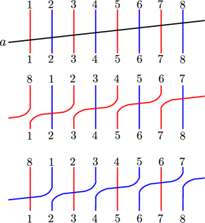
Figure 7: Graphical illustration of transfer matrices $t(u)$, $t(\mu)$ and $t(\nu)$. The corresponding spectral parameters of black, red and blue lines are $u$, $\mu$ and $\nu$, respectively. The line avoidings are a result of the regularity condition (III.5).

On a chain of length $L=2k$ we build an inhomogeneous transfer matrix with alternating inhomogeneities $\mu,\nu$ as

$$t(u)=\text{Tr}_{a}\Big{[}R_{a,L}(u,\nu)R_{a,L-1}(u,\mu)\dots{\\ }\dots R_{a,2}(u,\nu)R_{a,1}(u,\mu)\Big{]}.$$ (IV.3)

Using the regularity condition (III.5) we obtain two special points for the transfer matrix, where it becomes a product of distinct quantum gates multiplied by an overall translation (see figure 7)

$$t(\mu) =\mathcal{U}\check{R}_{L-1,L}(\mu,\nu)\dots\check{R}_{1,2}(\mu,\nu),$$ (IV.4)

$$t(\nu) =\mathcal{U}\check{R}_{L,1}(\nu,\mu)\dots\check{R}_{2,3}(\nu,\mu).$$ (IV.5)

Let us assume that the inversion relation (III.6) holds without scalar factors

$$\check{R}_{1,2}(u,v)\check{R}_{1,2}(v,u)=1.$$ (IV.6)

Then we obtain

$$(t(\nu))^{-1}=\check{R}_{L,1}(\mu,\nu)\dots\check{R}_{2,3}(\mu,\nu)\mathcal{U}^{-1}.$$ (IV.7)

Finally we see that the operator product

$$(t(\nu))^{-1}t(\mu)$$ (IV.8)

can be interpreted as a period-2 Floquet cycle of the form (II.11) with a two-site gate

$$U^{(2)}(j)=\check{R}_{j,j+1}(\mu,\nu),$$ (IV.9)

see figure 8.

The requirement of unitarity puts constraints on the $R$-matrix and the spectral parameters $\mu,\nu$. However, in the typical cases there are simple choices which fulfill unitarity, which depend on the real analyticity of the $R$-matrix. It follows from (IV.6) that the $R$-matrix is unitary for a pair $\mu,\nu$ if

$$\left(\check{R}_{1,2}(\mu,\nu)\right)^{\dagger}=\check{R}_{1,2}(\nu,\mu).$$ (IV.10)

In the simple case of the XXZ spin chain with $\Delta=\cosh(\eta)$ we can choose the following representation of the $R$-matrix:

$$\check{R}(\mu,\nu)=\begin{pmatrix}1&&&\\ &c(\mu-\nu)&b(\mu-\nu)&\\ &b(\mu-\nu)&c(\mu-\nu)&\\ &&&1\\ \end{pmatrix}$$ (IV.11)

with

$$c(u)=\frac{\sinh(\eta)}{\sinh(u+\eta)},\qquad b(u)=\frac{\sinh(u)}{\sinh(u+\eta)}.$$ (IV.12)

It can be seen that $\check{R}(\mu,\nu)$ is unitary if either $\eta$ is real ($\Delta>1$) and $\mu-\nu$ is purely imaginary, or if $\eta$ is purely imaginary ($\Delta<1$) and $\mu-\nu$ is real.

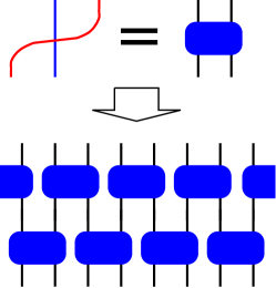
Figure 8: Graphical illustration of the period-2 Floquet cycle $(t(\nu))^{-1}t(\mu)$.

IV.2 Integrable quantum circuits for three-site models – Construction 1

Now we construct quantum circuits for the three site interacting models, which can be applied for every model which fits into our framework laid out in Section III. The specific case of the IRF type models is treated later in V.1, where we present a different type of quantum circuit adapted to the special form of those Lax operators.

We present two different Floquet circles for the three site models. In the first case we generalize the results from the previous Subsection to the present case: this is a rather straightforward construction from a technical point of view, but it leads to brickwork circuits with “untouched” sites. An alternative construction is presented in the next Subsection. That one leads to a tightly packed brickwork circuit, but its integrability structure is more involved.

In the first case we use the glued chain, where we group together pairs of sites of the original chain, see the derivations in Section III.2. Then the idea is to generalize the definition (IV.3) to the present case with the grouped sites. This way we obtain a quantum circuit with 4-site unitaries, because the $R$-matrix of the glued chain acts on pairs of sites. However, at special points we can make use of the factorization (III.29) in order to obtain the three site unitaries.

We take a chain of length $L=4k$ and construct an inhomogeneous transfer matrix for the grouped sites with alternating inhomogeneities $\mu,\nu$:

$$t(u)=\text{Tr}_{ab}\big{[}R_{(a,b)(4k-1,4k)}(u,\nu)\dots{\\ }\dots R_{(a,b)(3,4)}(u,\nu)R_{(a,b)(1,2)}(u,\mu)\big{]}$$ (IV.13)

Here $a,b$ stand for the two auxiliary spaces of the model. This family of transfer matrices is commuting. Special points are $u=\mu,\nu$ with

$$\begin{split}t(\mu)&=\mathcal{U}^{2}\check{R}_{(4k-3,4k-2)(4k-1,4k)}(\mu,\nu)\dots\check{R}_{(1,2)(3,4)}(\mu,\nu),\\ t(\nu)&=\mathcal{U}^{2}\check{R}_{(4k-1,4k)(1,2)}(\nu,\mu)\dots\check{R}_{(3,4)(5,6)}(\nu,\mu).\\ \end{split}$$ (IV.14)

Note the appearance of $\mathcal{U}^{2}$, the translation operator by two sites.

Similar to the nearest neighbor case, we take now the inverse of $t(\mu)$, which becomes

$$t^{-1}(\nu)=\check{R}_{(4k-1,4k)(1,2)}(\mu,\nu)\dots\check{R}_{(3,4)(5,6)}(\mu,\nu)\mathcal{U}^{-2}.$$ (IV.15)

Finally we define the Floquet cycle as

$$\mathcal{V}=t^{-1}(\nu)t(\mu)=\\ =\check{R}_{(4k-1,4k)(1,2)}(\mu,\nu)\dots\check{R}_{(3,4)(5,6)}(\mu,\nu)\times\\ \times\check{R}_{(4k-3,4k-2)(4k,4k-1)}(\mu,\nu)\dots\check{R}_{(1,2)(3,4)}(\mu,\nu).$$ (IV.16)

This can be understood as a cycle with period $\tau=2$ and with the four site gates

$$U^{(4)}(j)=\check{R}_{(j,j+1)(j+2,j+3)}(\mu,\nu).$$ (IV.17)

The coordinates of the gates are $x_{k}=4k$ and the displacements are $\Delta_{l}=2l$ with $l=1,2$. Similar to the nearest neighbor cases we need to impose restrictions on $\mu,\nu$ to obtain a gate which is unitary. This restriction depends on the model.

A quantum circuit with three site gates is obtained by substituting $\nu=0$. Then we use the factorization

$$\check{R}_{(j,j+1),(j+2,j+3)}(\mu,0)=\check{\mathcal{L}}_{j+1,j+2,j+3}(\mu)\check{\mathcal{L}}_{j,j+1,j+2}(\mu).$$ (IV.18)

which follows from (III.29). For a graphical interpretation of this relation see Figure 10.

Figure 9: Graphical illustration of operators $\check{\mathcal{L}}_{123}$ and $\mathcal{L}_{123}$.

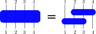
Figure 10: Graphical illustration of eq. (IV.18).

Substituting this factorization into (IV.16) we obtain a Floquet cycle with period $\tau=4$, three-site gates

$$U^{(3)}(j)=\check{\mathcal{L}}_{j,j+1,j+2}(\mu),$$ (IV.19)

coordinates $x_{k}=4k$ and displacements $\Delta_{l}=l$ with $l=1,2,3,4$. For a graphical interpretation of this quantum circuit see Figure 11.

Figure 11: In the top of the figure we can see the period 2 Floquet cycle for the glued chain. We changed the $R$-matrices from Fig. 8 to $\check{R}_{(12),(34)}(\mu,\nu)$. In the bottom we substitute $\nu=0$ and use the factorization property (IV.18). Thus we get a period 4 Floquet cycle with 3-site gates so that every fourth spin is untouched at every step.

Disadvantages of this construction are that the quantum circuit does not have left-right symmetry, and that the three-site unitaries are not tightly packed: every fourth spin is left untouched at every time step.

IV.3 Integrable quantum circuits for three-site models – Construction 2

Now we also present a quantum circuit which is tightly packed. We take three site gates defined by (IV.19) and construct a circuit with period $\tau=3$, coordinates $x_{k}=3k$ and displacements $\Delta_{l}=l$ with $l=1,2,3$. For a graphical interpretation see Fig. 12.

Figure 12: A tightly packed quantum circuit with three site gates. This network has periodicity 3 in both the space and time directions. Accordingly, we can prove the existence of commuting transfer matrices built from three rows.

Figure 13: Graphical interpretation of diagonal to diagonal transfer matrices, which are identical to those defined in (III.35), but drawn simply in a different arrangement, compare also with Fig. 5. This transfer matrix can also be used to build the circuit shown in 12, this was first worked out in [81].

Such a circuit was already introduced in [81], however, the integrability was only shown for the diagonal-to-diagonal transfer matrices, which are identical to the ones defined by (III.35) (for a pictorial interpretation see Fig. 13). Now we also develop the commuting row-to-row transfer matrices for this quantum circuit.

We start with the three site Lax operator $\check{\mathcal{L}}(u)$ and the associated $R$-matrix $\check{R}_{ab,(j,j+1)}(u,v)$. We construct an operator acting on 5 spaces

$$\check{\mathcal{R}}_{1,2,3,4,5}(\theta,u) =\check{\mathcal{L}}^{-1}_{1,2,3}(u)\check{R}_{2,3,4,5}(\theta,u)\check{\mathcal{L}}_{1,2,3}(\theta)$$

$$=\check{\mathcal{L}}_{3,4,5}(\theta)\check{R}_{1,2,3,4}(\theta,u)\check{\mathcal{L}}^{-1}_{3,4,5}(u).$$ (IV.20)

For the transfer matrices we will also need an operator which acts on one more space with a permutation, therefore we define

$$\mathcal{R}_{(1,2,3),(4,5,6)}(\theta,u)=\mathcal{P}_{1,4}\mathcal{P}_{2,5}\mathcal{P}_{3,6}\check{\mathcal{R}}_{1,2,3,4,5}(\theta,u).$$ (IV.21)

This matrix satisfies the YB equation

$$\mathcal{R}_{(1,2,3),A}(\theta,u)\mathcal{R}_{(1,2,3),B}(\theta,v)\mathcal{R}_{A,B}(u,v)=\\ \mathcal{R}_{A,B}(u,v)\mathcal{R}_{(1,2,3),B}(\theta,v)\mathcal{R}_{(1,2,3),A}(\theta,u),$$ (IV.22)

where $A=(4,5,6)$ and $B=(7,8,9)$ stand for additional two triplets of auxiliary spaces. Relation (IV.22) can be checked by direct substitution of the definitions above, and making use of the RLL relations (III.3) and YB relations (III.4) applied to the $R$-matrix in question.

Then we a construct a transfer matrix for our chain after grouping together triplets of physical spaces. The precise formula with auxiliary space $A=(a,b,c)$ reads

$$t(u)=\mathrm{tr}_{A}\bigl{[}\mathcal{R}_{(1,2,3),A}(\theta,u)\mathcal{R}_{(4,5,6),A}(\theta,u)\dots{\\ }\mathcal{R}_{(L-5,L-4,L-3),A}(\theta,u)\mathcal{R}_{(L-2,L-1,L),A}(\theta,u)\bigr{]}.$$ (IV.23)

Note that the relative ordering of the physical triplets is such that we proceed backwards on the chain, as in (III.10). This is due to certain technical details, so that in the end we can obtain the desired quantum circuit.

These transfer matrices commute, if we regard $\theta$ as a fixed parameter. The special point $u=\theta$ gives the translation operator by three sites:

$$t(\theta)=\mathcal{U}^{-3}.$$ (IV.24)

The other special point is obtained by setting $u=0$. In this case we get

$$t(\theta)^{-1}t(0)=\mathcal{V}_{3}\mathcal{V}_{2}\mathcal{V}_{1}.$$ (IV.25)

where the equal time update steps $\mathcal{V}_{j}$ are defined by

$$\mathcal{V}_{j}=\prod_{k}U^{(3)}(3k+j),\quad U^{(3}(j)=\check{\mathcal{L}}_{j,j+1,j+2}(\theta).$$ (IV.26)

For the proof of the initial condition (IV.25) we need to use the factorization condition (III.29) which eventually leads to

$$\check{\mathcal{R}}_{1,2,3,4,5}(\theta,0)=\check{\mathcal{L}}_{3,4,5}(\theta)\check{\mathcal{L}}_{2,3,4}(\theta)\check{\mathcal{L}}_{1,2,3}(\theta),$$ (IV.27)

where we also used the initial condition $\check{\mathcal{L}}_{1,2,3}(0)=1$. A graphical interpretation of this equation (applied for the six-site object $\mathcal{R}_{1,2,3,4,5,6}$) is given in Fig 14. Multiplying the operators thus obtained, together with the permutations introduced in (IV.21) will eventually lead to (IV.25). A graphical proof is shown on Fig. 15.

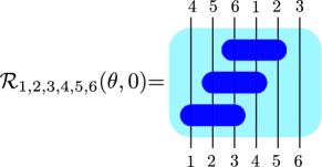
Figure 14: Graphical representation for the factorization of $\mathcal{R}_{1,2,3,4,5,6}(\theta,0)$ into the three site gates given by $\mathcal{L}(\theta)$. Note that the last vector space is also involved in the permutations, which is necessary in order to build the desired transfer matrix.

Figure 15: Graphical proof of eq. (IV.25). The labels $(a,b,c)$ stand for the triplet of auxiliary spaces which are present in the definition (IV.23). The big lightly shaded rectangles stand for the action of the $\mathcal{R}$ operators. Within each big rectangle we denoted the factorization into the product of $\mathcal{L}$ operators, as shown in Fig. 14. Then the quantum circuit of Fig. 12 is obtained by “straightening out” the angles of the three site gates, noticing that they perfectly fit together to build the tightly packed circuit. Notice that this circuit also inlcudes a translation by 3 sites, which is canceled by $t^{-1}(\theta)=\mathcal{U}^{3}$ in (IV.25).

V Interaction-round-a-face type models

In this Section we study the IRF type models. Our motivations come from recent results in the literature about elementary cellular automata, see the discussion in Section II.7. It is our goal to embed these models into the algebraic framework of medium range models. We will see that the special structure of these models leads to unique constructions for the quantum circuits, and also to the discovery of new algebraic structures that are connected to the “face weight formulation” of the Yang-Baxter relation.

We are looking for three site integrable models where the Lax operator has the special form

$$\check{\mathcal{L}}_{j,j+1,j+2}(u)=\sum_{a,b=0,1}P_{j}^{a}f^{ab}_{j+1}(u)P^{b}_{j+2},$$ (V.1)

where $f^{ab}(u)$ is a collection of four $u$-dependent matrices. Such Lax operators will be used to build quantum circuits: they will play the role of the three-site unitaries $U^{(3)}(j)$. The assumption (V.1) leads to unique algebraic constructions and quantum circuits, which would be meaningless without the special structure of the Lax operator.

Later in Subsection V.2 we perform a classification of such models, and in V.3 we also discuss the concrete cases that eventually lead to the elementary cellular automata.

V.1 Integrability structures and quantum circuits

In general we have $R$- and Lax-matrices which satisfy the $RLL$ relation which we now write in the form

$$\check{R}_{23,45}(u,v)\check{\mathcal{L}}_{123}(u)\check{\mathcal{L}}_{345}(v)=\\ =\check{\mathcal{L}}_{123}(v)\check{\mathcal{L}}_{345}(u)\check{R}_{12,34}(u,v).$$ (V.2)

It follows from (V.1) that now the Lax-operators satisfy an extra condition

$$[\check{\mathcal{L}}_{123}(u),\check{\mathcal{L}}_{345}(v)]=0.$$ (V.3)

Using this requirement the $RLL$ relation reads as

$$\check{\mathcal{L}}_{345}(u)^{-1}\check{R}_{23,45}(u,v)\check{\mathcal{L}}_{345}(v)=\\ \check{\mathcal{L}}_{123}(v)\check{R}_{12,34}(u,v)\check{\mathcal{L}}_{123}(u)^{-1}.$$ (V.4)

We can see that the l.h.s. and the r.h.s. act trivially on the spaces $1$ and $5$ respectively, therefore they have to be equal to a three-site operator which we denote as $\check{\mathcal{G}}_{234}$. Thus we find

$$\check{\mathcal{G}}_{234}(u,v) =\check{\mathcal{L}}_{345}(u)^{-1}\check{R}_{23,45}(u,v)\check{\mathcal{L}}_{345}(v),$$ (V.5)

$$\check{\mathcal{G}}_{234}(u,v) =\check{\mathcal{L}}_{123}(v)\check{R}_{12,34}(u,v)\check{\mathcal{L}}_{123}(u)^{-1}.$$ (V.6)

We can express the $R$-matrices with $\mathcal{G}$ and $\mathcal{L}$ in two ways:

$$\check{R}_{12,34}(u,v) =\check{\mathcal{L}}_{123}(v)^{-1}\check{\mathcal{G}}_{234}(u,v)\check{\mathcal{L}}_{123}(u),$$ (V.7)

$$\check{R}_{23,45}(u,v) =\check{\mathcal{L}}_{345}(u)\check{\mathcal{G}}_{234}(u,v)\check{\mathcal{L}}_{345}(v)^{-1},$$ (V.8)

or equivalently

$$\check{R}_{12,34}(u,v)=\check{\mathcal{L}}_{234}(u)\check{\mathcal{G}}_{123}(u,v)\check{\mathcal{L}}_{234}(v)^{-1}.$$ (V.9)

The consistency of the two expressions for the $R$-matrix leads to the equation

$$\check{\mathcal{G}}_{234}(u,v)\check{\mathcal{L}}_{123}(u)\check{\mathcal{L}}_{234}(v)=\\ =\check{\mathcal{L}}_{123}(v)\check{\mathcal{L}}_{234}(u)\check{\mathcal{G}}_{123}(u,v).$$ (V.10)

This relation is similar to eq. (V.2), but there are important differences: Here the supports for the Lax operators overlap at two spaces at both the l.h.s. and the r.h.s., whereas in (V.2) they overlap only at a single space. We call this equation the GLL relation. Below we show that it is equivalent to the “face weight” formulation of the RLL relation.

We can easily calculate this $G$-operator at special values of spectral parameters. Using the regularity of the $R$-matrix and eq. (V.5) we get

$$\check{\mathcal{G}}_{123}(v,v)=1.$$ (V.11)

Using the factorization of the $R$-matrix and eqs. (V.9) and (V.7) we obtain that

$$\check{\mathcal{G}}_{123}(u,0) =\check{\mathcal{L}}_{123}(u),$$ (V.12)

$$\check{\mathcal{G}}_{123}(0,v) =\check{\mathcal{L}}_{123}(v)^{-1}.$$ (V.13)

From (V.5) we can also derive the inversion property of the $G$-operator

$$\check{\mathcal{G}}_{123}(u,v)\check{\mathcal{G}}_{123}(v,u)=1.$$ (V.14)

The equations (V.9),(V.7),(V.5) and (V.6) imply that the $R$- and $G$-operators act diagonally on the first and last sites.

We also know that the $R$-matrix satisfies the YB equation

$$\check{R}_{34,56}(u_{1},u_{2})\check{R}_{12,34}(u_{1},u_{3})\check{R}_{34,56}(u_{2},u_{3})=\\ \check{R}_{12,34}(u_{2},u_{3})\check{R}_{34,56}(u_{1},u_{3})\check{R}_{12,34}(u_{1},u_{2}).$$ (V.15)

Substituting (V.9),(V.7) we can easily show that the $G$-operator also satisfies a YB type equation

$$\check{\mathcal{G}}_{234}(u_{1},u_{2})\check{\mathcal{G}}_{123}(u_{1},u_{3})\check{\mathcal{G}}_{234}(u_{2},u_{3})=\\ \check{\mathcal{G}}_{123}(u_{2},u_{3})\check{\mathcal{G}}_{234}(u_{1},u_{3})\check{\mathcal{G}}_{123}(u_{1},u_{2}).$$ (V.16)

Below we show that this is equivalent to the “face weight” formulation of the Yang-Baxter relation.

To see this we introduce a new notation for the Lax operator, by making use of its special form:

$$\check{\mathcal{L}}(u)=\sum_{i,j,k,l}M_{kj}^{il}(u)P_{i}\otimes E_{\>k}^{l}\otimes P_{j}.$$ (V.17)

Assuming that the $G$-operator has a similar form we write it as

$$\check{\mathcal{G}}(u,v)=\sum_{a,b,c,d}(g_{bc})_{d}^{a}(u,v)P_{a}\otimes E_{\>b}^{c}\otimes P_{d}.$$ (V.18)

Then the GLL relation is expressed as

$$\sum_{s}(g_{bs})_{r}^{i}(u,v)M_{sj}^{il}(u)M_{rq}^{sj}(v)=\\ \sum_{s}M_{bs}^{il}(v)M_{rq}^{bs}(u)(g_{sj})_{q}^{l}(u,v),$$ (V.19)

which is a relation used in [76]. This connection will be discussed further in Section V.4.

Let us now focus on the quantum circuits. We intend to build brickwork circuits which can accommodate the elementary cellular automata. It is clear that the constructions discussed in Section IV are not appropriate for this purpose, because there the local unitaries are too far away from each other. Instead, we need to build “tightly packed” quantum circuits where every pair of neighboring quantum gates is overlapping at the common control bit. This will enable us to treat some of the elementary cellular automata discussed in Section II.7.

Motivated by the discussion in Section II.7 we build a Floquet-type time evolution operator as

$$\mathcal{V}=\mathcal{V}_{2}\mathcal{V}_{1},$$ (V.20)

where the operators $\mathcal{V}_{1,2}$ are built from three site unitaries that we choose as

$$U^{(3)}(j)=\check{\mathcal{L}}_{j,j+1,j+2}(\theta)$$ (V.21)

The number $\theta$ will be a fixed parameter of the quantum circuit.

The update steps are then given by

$$\begin{split}\mathcal{V}_{1}&=\check{\mathcal{L}}_{1,2,3}(\theta)\check{\mathcal{L}}_{3,4,5}(\theta)\dots\check{\mathcal{L}}_{L-3,L-2,L-1}(\theta)\check{\mathcal{L}}_{L-1,L,1}(\theta)\\ \mathcal{V}_{2}&=\check{\mathcal{L}}_{2,3,4}(\theta)\check{\mathcal{L}}_{4,5,6}(\theta)\dots\check{\mathcal{L}}_{L-2,L-1,L}(\theta)\check{\mathcal{L}}_{L,1,2}(\theta).\end{split}$$ (V.22)

Notice that every pair of neighboring Lax operators overlaps at a common site. For a graphical interpretation see see Fig. 16.

The complete Floquet time step can be expressed alternatively as

$$\mathcal{V}=\mathcal{U}^{2}\mathrm{tr}_{ab}\bigl{[}\mathcal{L}_{1,2,b}\mathcal{L}_{1,2,a}\mathcal{L}_{3,4,b}\mathcal{L}_{3,4,a}\dots{\\ }\mathcal{L}_{L-3,L-2,b}\mathcal{L}_{L-3,L-2,a}\mathcal{L}_{L-1,L,b}\mathcal{L}_{L-1,L,a}\bigr{]}.$$ (V.23)

For simplicity we suppressed the dependence on $\theta$. For a graphical proof of the rewriting see Fig. 17.

Figure 16: Lax representation of the time evaluation operator $\mathcal{V}_{2}$.

Figure 17: Lax representation of the time evaluation operator $\mathcal{V}_{2}\mathcal{V}_{1}$.

We can now use the factorization of the $R$-matrix, which we write in the form

$$R_{(12),(34)}(\theta,0)=\mathcal{L}_{1,2,4}(\theta)\mathcal{L}_{1,2,3}(\theta).$$ (V.24)

Using this relation we can express the Floquet update step as

$$\mathcal{V}=\mathcal{U}^{2}\mathrm{tr}_{A}\bigl{[}R_{(1,2),A}(\theta,0)R_{(3,4),A}(\theta,0)\dots{\\ }R_{(L-3,L-2),A}(\theta,0)R_{(L-1,L),A}(\theta,0)\bigr{]},$$ (V.25)

where $A=(a,b)$ stands for a pair of auxiliary spaces. Defining the transfer matrix

$$t(u)=\mathrm{tr}_{A}\bigl{[}R_{(1,2),A}(\theta,u)R_{(3,4),A}(\theta,u)\dots{\\ }R_{(L-3,L-2),A}(\theta,u)R_{(L-1,L),A}(\theta,u)\bigr{]}$$ (V.26)

we obtain that

$$\mathcal{V}=t(\theta)^{-1}t(0),$$ (V.27)

where we used that

$$t(\theta)=\mathcal{U}^{-2}.$$ (V.28)

The transfer matrices (V.26) form a commuting family:

$$[t(u),t(v)]=0.$$ (V.29)

The variable $\theta$ plays the role of an inhomogeneity parameter for this commuting family. Note that (V.26) is a generalization of (III.10), and not of (III.9).

We can also define the rapidity dependent update rule

$$\mathcal{V}(u)=t(\theta)^{-1}t(u).$$ (V.30)

Clearly, these operators commute with each other, and thus they commute also with the “physical” update step which is obtained at $u=0$.

The operators $\mathcal{V}(u)$ are non-local for generic $u$. However, similar to the case of a standard transfer matrix they lead to extensive and local charges. The initial condition $\mathcal{V}(\theta)=1$ and the definition of the transfer matrix $t(u)$ lead to the extensive four-site operator

$$Q^{\prime}_{4}=\left.\partial_{u}\mathcal{V}(u)\right|_{u=\theta}.$$ (V.31)

The transfer matrix is only two-site invariant, which is inherited by $Q_{4}^{\prime}$. Therefore $Q_{4}^{\prime}$ is not translationally invariant, similar to the update rule $\mathcal{V}$ which is not translationally invariant either.

Higher charges could be obtained from the derivative of the logarithm of the transfer matrix, or with the boost operator method [93] applied to transfer matrix (V.26).

Figure 18: Graphical illustration of the transfer matrix (V.26). The blue, red and green boxes are the operators $\check{\mathcal{L}}(\theta)$, $\check{\mathcal{G}}(\theta,u)$ and $\check{\mathcal{L}}(u)^{-1}$, respectively. We use the commutativity (V.3) to separate the action of the upper (blue) layer of gates. However, the lower layer can not be simplified further, because there the consecutive operators overlap at two sites each.

Simplified formulas for the transfer matrix can be obtained using the $\check{\mathcal{G}}$ operators introduced above. We substitute the expression

$$\check{R}_{12,34}(\theta,u)=\check{\mathcal{L}}_{234}(\theta)\check{\mathcal{G}}_{123}(\theta,u)\check{\mathcal{L}}_{234}(u)^{-1}$$ (V.32)

into the definition (V.26). This substitution is depicted pictorially in the top of the figure 18. We can see here that the transfer matrix can be written as

$$t(u)=\mathcal{V}_{2}\tilde{t}(u),$$ (V.33)

where

$$\tilde{t}(u)=\\ \mathrm{tr}_{a,b}\bigl{[}\mathcal{G}_{1,a,b}(\theta,u)\mathcal{L}_{2,a,b}(u)^{-1}\mathcal{G}_{3,a,b}(\theta,u)\mathcal{L}_{4,a,b}(u)^{-1}\dots{\\ }\mathcal{G}_{L-1,a,b}(\theta,u)\mathcal{L}_{L,a,b}(u)^{-1}\bigr{]}.$$ (V.34)

For this rewriting we used again the fact that the $\check{\mathcal{L}}$ operators commute if they share a control bit.

The operator $\tilde{t}(u)$ is completely identical with the transfer matrices defined in [76], which can be seen after proper identifications are made. To this order we need to use the representations (V.17) and (V.18) for the $\check{\mathcal{L}}$ and $\check{\mathcal{G}}$ matrices. After substitution we obtain a formula identical to the one presented in [76], see eq. (V.66) below.

Our derivation in this Subsection assumed the regularity condition for the $R$-matrix, which leads to the factorization (V.24). However, an alternative derivation is also possible, without this assumption. We could start with the definition (V.26) for a proper $R$-matrix, and we then could still derive the alternative form (V.33). In concrete cases it could be shown that this transfer matrix is related to cellular automata. Such a derivation would completely bypass the requirement of the regularity. However, in this work we are interested in cases which yield local conserved charges. Furthermore we found that if the regularity condition does not hold then the concrete models do not have more conserved charges at all, see the example of the Rule54 model in V.4. Therefore we do not discuss solutions without the regularity condition.

V.2 Partial classification

Here we perform a partial classification of three site models, where the Lax operators have the special structure (V.1). The methods for the classification are essentially the same as in Section III. We are looking for Lax operators satisfying the RLL relations, and we perform a classification based on the Hamiltonian densities that are derived from the Lax operators: we apply the generalized Reshetikhin condition to find the integrable cases.

It is important the Hamiltonians that we find this way don’t commute with the transfer matrices defined in the previous Subsection, because the transfer matrices involve the inhomogeneities as well. The Hamiltonians only commute with homogeneous transfer matrices as defined in (III.24). However, we can also regard the Hamiltonians we find below as new integrable models on their own right.

It follows from the Ansatz (V.1) and the derivation rule (III.40) that the Hamiltonians in question have the structure given by (III.53) with the action matrices being

$$h^{ab}=\left.\partial_{u}f^{ab}(u)\right|_{u=0}.$$ (V.35)

Therefore we need to classify three-site Hamiltonians with the particular structure given by (III.53), where the outer two spins act as control bits, and the middle spin is an action bit. For this special class of models we assume that the inversion relation (III.19) holds, therefore we exclude the possibility of having a non-zero $\tilde{h}_{j,j+1,j+2}$ in the construction of $Q_{5}$, see (II.10).

The Ansatz (III.53) has a total number of 16 real parameters, because there are 4 $g$-matrices which are Hermitian. Subtracting the identity component and performing a $U(1)$ rotation the number of parameters could be narrowed down to 14. However, we found this parameter space to be too big for a first classification attempt. Instead, we selected an even more restricted Ansatz given explicitly by

$$h_{123}=A\sigma^{x}_{2}+B\sigma^{z}_{2}+C\sigma^{z}_{1}\sigma^{x}_{2}+D\sigma^{x}_{2}\sigma^{z}_{3}+\\ +E\sigma^{z}_{1}\sigma^{z}_{2}\sigma^{z}_{3}+F\sigma^{z}_{1}\sigma^{x}_{2}\sigma^{z}_{3}+G\sigma^{z}_{1}\sigma^{z}_{3}.$$ (V.36)

Apart from an overall multiplicative normalization this Ansatz has 6 free parameters, which makes the classification of integrable cases relatively easy. A Hermitian operator is obtained if all parameters are real, and in this case all matrix elements are real in the computational basis.

Within this parameter space we found three non-trivial integrable models. Now we list these models together with a brief discussion of their main properties. Their application as quantum gate models and classical cellular automata is discussed later in Subsection V.3; here we focus on their properties as integrable Hamiltonians.

We put forward that two of the models can be related to nearest neighbor chains by a bond-site transformation. This transformation was used recently in [54, 81] and it is explained in detail in Appendix B.

V.2.1 The bond-site transformed XYZ model

In this case the Hamiltonian density is written in the compact form

$$h_{123}=J_{x}\sigma^{x}_{2}-J_{y}\sigma^{z}_{1}\sigma^{x}_{2}\sigma^{z}_{3}+J_{z}\sigma^{z}_{1}\sigma^{z}_{3}.$$ (V.37)

This model can be seen as the bond-site transformed version of the XYZ model (we suggest to call it the bXYZ model). The Hamiltonian satisfies the requirements of the bond-site transformation discussed in Appendix B: it is spin reflection invariant and the first and last bits are control bits. Using the formulas (B.2) for the transformation of the operators we see immediately that in the bond picture the model becomes identical to the XYZ model with the couplings as given above. Thus it describes interacting dynamics of Domain Walls, where the creation and annihilation of pairs of DW’s is also allowed.

A special point of the model is when $J_{x}=J_{y}$, which becomes the bond-site transformation of the XXZ model. In this case the Hamiltonian commutes with the $U(1)$-charge

$$Q_{2}=\sum_{j}\sigma^{z}_{j}\sigma^{z}_{j+1},$$ (V.38)

which is interpreted as the Domain Wall number, which is conserved. This model was already presented in [101, 56].

An other special case is when $J_{y}=0$. In this case the model describes two decoupled quantum Ising chains on the even and odd sub-lattices, such that the parameter $J_{x}$ can be interpreted as a magnetic field. Switching on $J_{y}\neq 0$ we obtain a Bariev-type coupling between the two sub-lattices, therefore we could also call this system the Bariev-Ising model.

The Lax operator is found using the known solution for the XYZ model and the bond-site transformation:

$$\check{\mathcal{L}}_{1,2,3}(u)=\frac{1}{2}\frac{\mathrm{sn}(\eta)+\mathrm{sn}(u)\sigma_{2}^{x}}{\mathrm{sn}(\eta)+\mathrm{sn}(u)}(1-\sigma_{1}^{z}\sigma_{3}^{z})+\\ \frac{1}{2}\frac{\mathrm{sn}(u+\eta)+k\mathrm{sn}(\eta)\mathrm{sn}(u)\mathrm{sn}(u+\eta)\sigma_{2}^{x}}{\mathrm{sn}(\eta)+\mathrm{sn}(u)}(1+\sigma_{1}^{z}\sigma_{3}^{z}),$$ (V.39)

where $\mathrm{sn}(u)=\mathrm{sn}(u;k)$ and

$$\frac{J_{y}}{J_{x}}=\frac{1-k\mathrm{sn}^{2}(\eta)}{1+k\mathrm{sn}^{2}(\eta)}\qquad\frac{J_{z}}{J_{x}}=\frac{\mathrm{cn}(\eta)\mathrm{dn}(\eta)}{1+k\mathrm{sn}^{2}(\eta)}.$$ (V.40)

This Lax operator satisfies the inversion relation (III.49)

$$\check{\mathcal{L}}_{1,2,3}(u)\check{\mathcal{L}}_{1,2,3}(-u)=1.$$ (V.41)

In this model the $G$-operator can be obtained from the Lax operator in a very natural way

$$\check{\mathcal{G}}_{123}(u,v)=\check{\mathcal{L}}_{123}(u-v).$$ (V.42)

Taking $k\to 0$ we obtain the XXZ limit of the model

$$\check{\mathcal{L}}_{1,2,3}(u)=(P_{1}^{\circ}P_{3}^{\circ}+P_{1}^{\bullet}P_{3}^{\bullet})\frac{\sin(u+\eta)}{\sin(u)+\sin(\eta)}+\\ +(P_{1}^{\circ}P_{3}^{\bullet}+P_{1}^{\bullet}P_{3}^{\circ})\frac{\sin(u)\sigma^{x}_{2}+\sin(\eta)}{\sin(u)+\sin(\eta)}.$$ (V.43)

We can also take the XXX limit as $\eta\to 0$ and $u=\eta v$. We obtain the following Lax matrix

$$\check{\mathcal{L}}_{1,2,3}(v)=(P_{1}^{\circ}P_{3}^{\circ}+P_{1}^{\bullet}P_{3}^{\bullet})+\\ +(P_{1}^{\circ}P_{3}^{\bullet}+P_{1}^{\bullet}P_{3}^{\circ})\frac{v\sigma^{x}_{2}+1}{v+1}.$$ (V.44)

V.2.2 Twisted XX model with n.n.n. coupling

In this model the Hamiltonian density is

$$h_{123}=\sigma^{z}_{1}\sigma^{x}_{2}+\kappa\sigma^{x}_{2}\sigma^{z}_{3}+G\sigma^{z}_{1}\sigma^{z}_{3}.$$ (V.45)

These are actually two different models depending on the sign $\kappa=\pm 1$; the real parameter $G$ is a coupling constant. The form of the Hamiltonian density respects the Ansatz (V.36), but perhaps a more familiar way of writing the global Hamiltonian is

$$H=\sum_{j}\sigma^{x}_{j}\sigma^{y}_{j+1}\pm\sigma^{y}_{j}\sigma^{x}_{j+1}+G\sigma^{x}_{j}\sigma^{x}_{j+2}.$$ (V.46)

Here we performed a rotation such that the Pauli matrices are cyclically exchanged as $\sigma^{x}\to\sigma^{y}\to\sigma^{z}$. In the case of a minus sign we can further express this as

$$H=\sum_{j}2i(\sigma^{+}_{j}\sigma^{-}_{j+1}-\sigma^{-}_{j}\sigma^{+}_{j+1})+G\sigma^{x}_{j}\sigma^{x}_{j+2},$$ (V.47)

which can be interpreted as a twisted XX model with a next-to-nearest neighbor interaction term.

In the case of a plus sign in (V.45) we do not get such an interpretation.

An alternative interpretation of the model is found by performing a bond-site transformation. First we perform a transformation $\sigma^{x}\leftrightarrow\sigma^{y}$ so that the Hamiltonian density becomes

$$h_{123}=\sigma^{z}_{1}\sigma^{y}_{2}+\kappa\sigma^{y}_{2}\sigma^{z}_{3}+G\sigma^{z}_{1}\sigma^{z}_{3}.$$ (V.48)

This operator is spin flip invariant therefore we can apply the bond-site transformation discussed in Section B. Then we obtain a two site interacting model with Hamiltonian density

$$h_{12}=\sigma^{y}_{1}\sigma^{x}_{2}+\kappa\sigma^{x}_{1}\sigma^{y}_{2}+G\sigma^{z}_{1}\sigma^{z}_{2}.$$ (V.49)

If $\kappa=-1$, then the original Hamiltonian commutes with the $U(1)$-charge given by (V.38), and the model defined by (V.49) commutes with the global $S^{z}$ operator. In fact, this case can be interpreted as the XXZ model with a homogeneous twist, where the kinetic term is the Dzyaloshinskii–Moriya interaction term. Thus the model describes the interacting dynamics of the Domain Walls, with a twisted kinetic term.

For the model with $\kappa=1$ we did not find a translationally invariant $U(1)$-charge, and the kinetic term describes the creation and annihilation of pairs of Domain Walls.

We found the Lax operator for both models. It is given by

$$\check{\mathcal{L}}_{123}(u)=G\frac{e^{2u}-1}{(e^{u}-1)^{2}-4G^{2}}\times\\ \left(\frac{2G\kappa}{e^{u}-1}+\left(\sigma^{z}_{1}\sigma^{x}_{2}+\kappa\sigma^{x}_{2}\sigma^{z}_{3}\right)+\frac{e^{u}-1+2G^{2}}{G(e^{u}+1)}\sigma^{z}_{1}\sigma^{z}_{3}\right).$$ (V.50)

Relation (III.49) holds with this parametrization. This operator is unitary if $u$ is purely imaginary.

The $G$-operator (which immediately gives the $R$-matrix as well) reads as

$$\check{\mathcal{G}}_{123}(u,v)=\kappa\frac{(4G^{2}-1)e^{v}-e^{u}+e^{u}e^{v}+1}{2G(e^{u}-e^{v})}+\\ \left(\sigma^{z}_{1}\sigma^{x}_{2}+\kappa\sigma^{x}_{2}\sigma^{z}_{3}\right)+G\frac{(4G^{2}-3)e^{v}+e^{u}+e^{u}e^{v}+1}{(2G^{2}-1)(e^{u}+e^{v})+e^{u}e^{v}+1}\sigma^{z}_{1}\sigma^{z}_{3}.$$ (V.51)

Substituting the special point $G=1$ we get

$$\check{\mathcal{L}}_{123}(u)=\frac{e^{u}-1}{e^{u}-3}\times\\ \left(\frac{2\kappa}{e^{u}-1}+\left(\sigma^{z}_{1}\sigma^{x}_{2}+\kappa\sigma^{x}_{2}\sigma^{z}_{3}\right)+\sigma^{z}_{1}\sigma^{z}_{3}\right),$$ (V.52)

A special point is $u=i\pi$, at which the unitary operator becomes deterministic; this will lead to an elementary cellular automata, see Section V.3 below.

V.2.3 Integrable deformation of the PXP model

This model has no free parameters, just a sign $\kappa=\pm 1$:

$$h_{123}=\sigma^{x}_{2}+\kappa(\sigma^{z}_{1}\sigma^{x}_{2}+\sigma^{x}_{2}\sigma^{z}_{3})+\sqrt{2}\sigma^{z}_{1}\sigma^{z}_{2}\sigma^{z}_{3}-\sigma^{z}_{1}\sigma^{x}_{2}\sigma^{z}_{3}.$$ (V.53)

In the case of $\kappa=1$ the Hamiltonian density can be expressed as

$$h_{123}=-4P^{\bullet}_{1}\sigma^{x}_{2}P^{\bullet}_{3}+2\sigma^{x}_{2}+\sqrt{2}\sigma^{z}_{1}\sigma^{z}_{2}\sigma^{z}_{3},$$ (V.54)

while for $\kappa=-1$ we would obtain a similar model with $P^{\bullet}$ replaced by $P^{\circ}$. These models can be seen as an integrable deformation of the PXP model [102]. However, if we remain in the parameter space of our Ansatz, then there is no free parameter, so we can not tune the “operator distance” from the PXP Hamiltonian.

It is likely that the models (V.53) are just particular cases of a continuous family of models which stretches outside our Ansatz. We leave the exploration of the bigger parameter space to future works.

For this model we find the Lax operator

$$\check{\mathcal{L}}_{123}(u)=\frac{1+uh_{123}}{1+\sqrt{6}u}.$$ (V.55)

Simple computation shows that

$$(h_{123})^{2}=6.$$ (V.56)

This implies that (III.49) is satisfied. In this case a unitary gate is obtained for $u$ being purely imaginary.

For this specific model we did not find a bond-site transformation, which would make it locally equivalent to a n.n. chain.

V.3 Elementary cellular automata

The construction of Subsection V.1 can be applied for every IRF type 3-site model treated in Section V.2: this way we obtain families of quantum cellular automata with varying numbers of free parameters. All of these models are Yang-Baxter integrable. Now we are looking for specific cases that can accommodate the elementary cellular automata discussed in Section II.7.

First we consider the bXYZ model (V.37) at the special point $J_{x}=J_{y}=J_{z}$, in which case the Lax operator is given by (V.44). Taking the $v\to\infty$ limit we obtain the three site unitary

$$U^{(3)}(1)=(P^{\bullet}_{1}P^{\circ}_{3}+P^{\circ}_{1}P^{\bullet}_{3})\sigma^{x}_{2}+P^{\bullet}_{1}P^{\bullet}_{3}+P^{\circ}_{1}P^{\circ}_{3}.$$ (V.57)

We recognize that this is the update rule for the classical Rule150 model given by (II.21). Thus we obtained a Yang-Baxter integrable three parameter family of quantum cellular automata (with the parameters being $J_{y}/J_{x}$, $J_{z}/J_{x}$ and $v$, or alternatively $k$, $\eta$ and $v$), which includes the Rule150 model at special points. At this special point the first non-trivial local conserved charge is

$$Q^{\prime}_{4}=\sum_{j}\sigma_{2j}^{x}\sigma_{2j+1}^{x}+\sigma_{2j-1}^{z}\sigma_{2j}^{y}\sigma_{2j+1}^{y}\sigma_{2j+2}^{z}+\\ +\sigma_{2j-1}^{z}\sigma_{2j}^{z}\sigma_{2j+1}^{z}\sigma_{2j+2}^{z}.$$ (V.58)

Let us now perform the bond-site transformation of Appendix B directly on the quantum cellular automata. In the bond picture we obtain two-site gates that are given directly by the $R$-matrices of the XXX, XXZ and XYZ models. In the XXZ case the two-site gate is given by (IV.11), unitary time evolution is obtained if $\eta\in\mathbb{R}$ and $v\in i\mathbb{R}$ or vice versa. The classical Rule150 model is obtained after taking the special limits $\eta\to 0$ and $v\to\infty$, in which case the $R$-matrix (IV.11) becomes a permutation operator (swap gate). This implies that the Rule150 model describes free movement of Domain Walls. The XXZ version can be seen as an interacting deformation where the total number of DW’s is conserved. Finally the XYZ case is the most general model in this family, where Domain Walls can be created or annihilated in pairs.

Let us also consider the Model of Section V.2.2 with the sign $\kappa=1$ and the coupling constant $G=1$, for which the Lax operator and thus the three-site unitary is given by (V.52). Further substituting $u=i\pi$ we obtain

$$U^{(3)}(1)=\frac{1}{2}\left(-1+\sigma^{z}_{1}\sigma^{x}_{2}+\sigma^{x}_{2}\sigma^{z}_{3}+\sigma^{z}_{1}\sigma^{z}_{3}\right),$$ (V.59)

This is also a deterministic quantum gate, which gives the $f$ matrices

$$f^{00}=-f^{11}=\sigma^{x},\quad f^{01}=f^{10}=-1.$$ (V.60)

We can see that apart from simple signs these $f$-matrices are equal to those of the Rule105 model given by (II.20). As already argued in [81], if the quantum gates are deterministic, then the phases are irrelevant for the simulation of a classical cellular automata. Thus the two-parameter family of quantum gates (V.52) can be considered as a deformation of the actual Rule105 model, which is included at the special point $G=1$ and $u=i\pi$.

For this model and the specific values $G=1$ and $u=i\pi$ the definition (V.31) gives the local conserved charge

$$Q^{\prime}_{4}=\sum_{j}\sigma_{2j}^{y}\sigma_{2j+1}^{y}+\sigma_{2j-1}^{z}\sigma_{2j}^{x}\sigma_{2j+1}^{x}\sigma_{2j+2}^{z}+\\ +\sigma_{2j-1}^{z}\sigma_{2j}^{z}\sigma_{2j+1}^{z}\sigma_{2j+2}^{z}.$$ (V.61)

Performing the transformation $\sigma^{x}\leftrightarrow\sigma^{y}$ mentioned above we obtain the same charge as in (V.58).

The charges (V.58) and (V.61) commute with the time evolution of the update rules given by (II.21) and (V.60), respectively. The update rules are deterministic, therefore if we choose a “classical” initial state (an element of the computational basis) then it will stay classical. This also means that for the classical time evolution we can disregard the the $\sigma^{x}$ and $\sigma^{y}$ operators, because their mean values in the classical states are zero. This leads to the following classical charge for the Rule105 and Rule150 models:

$$Q^{(cl)}_{4}=\sum_{j}\sigma_{2j-1}^{z}\sigma_{2j}^{z}\sigma_{2j+1}^{z}\sigma_{2j+2}^{z}.$$ (V.62)

This charge is conserved by both classical cellular automata. Taking further derivatives of the logarithm of the transfer matrix we could obtain further quantum and classical charges for these models. If we consider the quantum models then the relative signs in (V.60) have to be taken into account. So far we have not yet found a quantum model which would describe the Rule105 model without these signs, but this could be just a limitation of our Ansatz (V.36).

Regarding the Rule54 and Rule201 models we did not find any three-site Hamiltonian, which would lead to Lax operators and transfer matrices that would actually accommodate these classical cellular automata. This is in accordance with the findings of [76]. Regarding the Rule54 model it was claimed in [76] that there are no translationally invariant local charges up to interaction range $\ell=5$. This clearly shows that for the Rule54 model we can not have a Lax operator acting on three sites, because it would give a translationally invariant charge $Q_{4}^{\prime}$ with range $\ell=4$. The alerted reader might object that our $Q_{4}^{\prime}$ derived in (V.31) is invariant with respect to a two site shift only. However, in the case of these cellular automata we also have the inversion relations (II.29) which implies that the two-site invariant charge $Q_{4}^{\prime}$ commuting with $\mathcal{V}_{2}\mathcal{V}_{1}$ has to commute with $\mathcal{V}_{1}\mathcal{V}_{2}$ as well, leading eventually to a translationally invariant version of $Q_{4}^{\prime}$ commuting with both $\mathcal{V}_{2}\mathcal{V}_{1}$ and $\mathcal{V}_{1}\mathcal{V}_{2}$. Altogether we reach the Conclusion that the Rule54 model is not Yang-Baxter integrable with three site interactions.

In Subsection V.4 below we also analyze the recent construction of [76] for these models, and we reach the same conclusion: the transfer matrices built in [76] only have a diagonal dressing using a known charge and thus do not lead to extra conserved charges.

However, it is known that there is a local conserved charge for the Rule54 model with interaction range $\ell=6$: it is the Hamiltonian derived in [74]. This suggests that perhaps the true algebraic background for the model lies within the family of 6-site interacting models. We return to this question in the Discussions (Section VII).

V.4 Discussion of the results of [76] for the IRF models

Recently an algebraic framework for the integrability of the Rule54 and related models was proposed in [76]. Here we review this construction, we point out connections with our results, and we also disprove some of the conjectures made in [76].

Let us start with a brief discussion of integrable 2D statistical physical models. There are three different sorts of commonly used models: spin models, vertex models, and interaction round a face (IRF) models. Accordingly, there are three different types of Yang-Baxter equations, one for each family. The different formulations can always be transformed into each other, although this might not be convenient and it can lead to an increase in the local dimensions. For a summary of the different formulations see the introductory Sections of [103, 104].

Nowadays the most commonly used formulation is the one based on vertex models; this is also what was used throughout the present work. It was a new idea of [76] to construct transfer matrices for the classical cellular automata (and for certain deformations thereof) using the IRF language.

Now we review the construction of [76], by focusing on the Rule54 model without deformation. We will show that the transfer matrices of [76] have an identical structure as in our quantum circuits discussed above.

The time evolution operator of [76] is built exactly in the same way as in (II.16)-(II.17) with the three site gates having the structure given by (II.15). Afterwards a commuting family of transfer matrices is built using two matrices $L^{j_{1},j_{2}}_{i_{1},i_{2}}(\lambda)$ and $M^{j_{1},j_{2}}_{i_{1},i_{2}}(\lambda)$ which describe face weights in the IRF language. Both matrices have four indices ranging from 1 to 2, and they can be represented most easily as $4\times 4$ matrices using the conventions for the tensor product:

$$L=\left(\begin{array}[]{cccc}L_{0,0}^{0,0}&L_{0,0}^{0,1}&L_{0,0}^{1,0}&L_{0,0}^{1,1}\\ L_{0,1}^{0,0}&L_{0,1}^{0,1}&L_{0,1}^{1,0}&L_{0,1}^{1,1}\\ L_{1,0}^{0,0}&L_{1,0}^{0,1}&L_{1,0}^{1,0}&L_{1,0}^{1,1}\\ L_{1,1}^{0,0}&L_{1,1}^{0,1}&L_{1,1}^{1,0}&L_{1,1}^{1,1}\end{array}\right).$$ (V.63)

The number $\lambda$ is interpreted again as a spectral parameter. The explicit form of the $L$ and $M$ matrices is given by

$$L(\lambda)=\begin{pmatrix}1&&1&\\ 1&&1&\\ &\lambda^{2}&&\lambda\\ &\lambda&&1\\ \end{pmatrix},$$ (V.64)

$$M(\lambda)=\begin{pmatrix}1&&1&\\ &1/\lambda&&1/\lambda\\ &1&1/\lambda&\\ 1&&1/\lambda&\\ \end{pmatrix}.$$ (V.65)

The transfer matrices $\mathcal{I}(\lambda)$ are defined component-wise as

$$\mathcal{I}^{j_{1},j_{2},\dots,L}_{i_{1},i_{2},\dots,i_{L}}(\lambda)=\prod_{x=1}^{L/2}M^{j_{2x-1},j_{2x}}_{i_{2x-1},i_{2x}}(\lambda)L^{j_{2x},j_{2x+1}}_{i_{2x},i_{2x+1}}(\lambda).$$ (V.66)

There is no summation over repeated indices.

It is then proven in [76] that the transfer matrices commute with each other and also with the time evolution operator:

$$[\mathcal{I}(\lambda),\mathcal{V}]=0.$$ (V.67)

This is shown using the “face weight” formulation of the Yang-Baxter relation discussed above.

This construction of [76] is completely identical with our quantum circuits of Section V.1 after proper identifications are made. It was already shown in Section V.1 that our GLL and GGG relations are identical to the “face weight” formulation of the Yang-Baxter relation given by eq. (V.19). Furthermore, we recognize the structural similarity between the transfer matrices (V.34) and (V.66). This leads to the following correspondences:

$$\check{\mathcal{L}}_{123}(\theta) \equiv f$$ (V.68)

$$\check{\mathcal{L}}_{123}(u) \equiv M$$ (V.69)

$$\check{\mathcal{G}}_{234}(\theta,u) \equiv L$$ (V.70)

$$\check{\mathcal{G}}_{123}(u_{1},u_{2}) \equiv g,$$ (V.71)

where on the l.h.s. we listed our operators, and the r.h.s. contains the objects defined in [76]. For the identification of the indices see eqs. (V.17) and (V.18).

Let us now show that in the particular case of the Rule54 model the transfer matrix (V.66) does not yield new conserved charges.

First of all we consider two known conserved operators in this model: the translation operator $\mathcal{U}$ and the particle current defined as

$$\mathcal{J}=\sum_{x=1}^{L/2}\big{(}\sigma^{z}_{2x-1}\sigma^{z}_{2x}-\sigma^{z}_{2x}\sigma^{z}_{2x+1}\big{)}.$$ (V.72)

This operator anti-commutes with both the shift and the single step update operators:

$$\{\mathcal{J},\mathcal{U}\}=\{\mathcal{J},\mathcal{V}_{1}\}=\{\mathcal{J},\mathcal{V}_{2}\}=0$$ (V.73)

It follows that it commutes with the Floquet-cycle operator $\mathcal{V}=\mathcal{V}_{2}\mathcal{V}_{1}$:

$$[\mathcal{J},\mathcal{V}]=0.$$ (V.74)

The translation operator intertwines the two update steps:

$$\mathcal{V}_{1}\mathcal{U}=\mathcal{U}\mathcal{V}_{2},$$ (V.75)

Strictly speaking $\mathcal{U}$ is not conserved by the Floquet cycle $\mathcal{V}$, because it interchanges the odd and even sites. On the other hand, $\mathcal{U}^{2}$ is conserved.

It was conjectured in [76] that new quasi-local charges can be obtained from the transfer matrix (V.66). On the contrary, we show here that $\mathcal{I}(\lambda)$ is functionally dependent on the time evolution operator and the two conserved operators $\mathcal{U}$ and $\mathcal{J}$.

First we note that the matrix $L^{j_{1},j_{2}}_{i_{1},i_{2}}(\lambda)$ is diagonal in the indices $j_{2}\leftrightarrow i_{1}$, and it can be factorized as

$$L^{j_{1},j_{2}}_{i_{1},i_{2}}(\lambda)=\delta_{i_{1},j_{2}}\lambda^{A^{j_{1}}_{i_{1}}+B^{j_{2}}_{i_{2}}},$$ (V.76)

where

$$A^{j_{1}}_{i_{1}}=\delta_{j_{1},0}\delta_{i_{1},1},\qquad B^{j_{2}}_{i_{2}}=\delta_{j_{2},1}\delta_{i_{2},0}.$$ (V.77)

The factorization above means that the $\lambda$-dependence can be separated into index pairs to the left and to the right. It follows that the transfer matrix (V.66) can be written as

$$\mathcal{I}^{j_{1},j_{2},\dots,j_{L}}_{i_{1},i_{2},\dots,i_{L}}(\lambda)=\prod_{x=1}^{L/2}\tilde{M}^{j_{2x-1},j_{2x}}_{i_{2x-1},i_{2x}}(\lambda)\delta_{i_{2x},j_{2x+1}},$$ (V.78)

where

$$\tilde{M}^{j_{1},j_{2}}_{i_{1},i_{2}}(\lambda)=\lambda^{B^{j_{1}}_{i_{1}}}M^{j_{1},j_{2}}_{i_{1},i_{2}}(\lambda)\lambda^{A^{j_{2}}_{i_{2}}}.$$ (V.79)

Once again there is no summation over repeated indices.

Furthermore, the same operator can be written as $\mathcal{I}(\lambda)=\mathcal{U}\tilde{\mathcal{I}}(\lambda)$, where now the components of $\tilde{\mathcal{I}}(\lambda)$ are

$$\tilde{\mathcal{I}}^{j_{1},j_{2},\dots,L}_{i_{1},i_{2},\dots,i_{L}}(\lambda)=\prod_{x=1}^{L/2}\tilde{M}^{j_{2x-2},j_{2x-1}}_{i_{2x-1},i_{2x}}(\lambda)\delta_{i_{2x},j_{2x}}.$$ (V.80)

We can see that this operator acts as the identity on the even sites, which become control bits for the action on the odd sites. To be more precise, the same operator can be written as a product of commuting three-site unitaries

$$\tilde{\mathcal{I}}(\lambda)=\prod_{x=1}^{L/2}U^{(3)}(2x|\lambda),$$ (V.81)

where $U^{(3)}(2x|\lambda)$ has the form of (II.15) with the $\lambda$-dependent $f$-matrices given through the matrix elements

$$\big{(}f^{ab}(\lambda)\big{)}_{i}^{j}=\tilde{M}^{aj}_{ib}(\lambda).$$ (V.82)

Considering the concrete components of $\tilde{M}$ we can write the individual $f$-matrices as

$$f^{11}=\sigma^{x},\quad f^{00}=1$$ (V.83)

and

$$f^{10}=\begin{pmatrix}\lambda&\\ &1/\lambda\end{pmatrix}\sigma^{x},\quad f^{01}=\begin{pmatrix}1/\lambda&\\ &\lambda\end{pmatrix}\sigma^{x}.$$ (V.84)

Comparing to (II.19) we see that these are $\lambda$-deformed versions of the original $f$-matrices of the model. Thus we can write

$$\tilde{\mathcal{I}}(1)=\mathcal{V}_{2},$$ (V.85)

where $\mathcal{V}_{1,2}$ are the two operators that define the update rules, see (II.16)-(II.17).

Collecting the factors of $\lambda$ as we multiply the equal time quantum gates we obtain

$$\tilde{\mathcal{I}}(\lambda)=\lambda^{\mathcal{J}/2}\ \mathcal{V}_{2},$$ (V.86)

where $\mathcal{J}$ is the particle current operator defined in (V.72). Going back to the actual transfer matrix we get

$$\mathcal{I}(\lambda)=\mathcal{U}\ \lambda^{\mathcal{J}/2}\ \mathcal{V}_{2}.$$ (V.87)

This formula means that the transfer matrix $\mathcal{I}(\lambda)$ is functionally dependent on three known operators: the cyclic shift, the conserved particle current, and the single step update rule. From this formula it follows that $\mathcal{I}(\lambda)$ is unitary if $|\lambda|=1$; this was an unexplained observation of [76]. Finally, for the product of two transfer matrices we obtain

$$\mathcal{I}(\lambda_{2})\mathcal{I}(\lambda_{1})=\mathcal{U}^{2}(\lambda_{1}\lambda_{2})^{-\mathcal{J}}\mathcal{V}.$$ (V.88)

Here we used the anti-commutation relations (V.73) and the definition of the Floquet cycle $\mathcal{V}$. This proves the commutativity of the transfer matrices. Furthermore, choosing $\lambda_{1}=\lambda_{2}$ we find that the squared transfer matrix is simply just a combination of the two-site translation, the conserved particle current, and the Floquet update rule.

We interpret this result as follows: Even though the Rule54 model seems integrable, the construction of [76] can not be considered as a proof of it, because [76] fails to introduce new charges on top of the existing ones. The same conclusion can be reached for the deformed Rule54 model, where the $M$-matrices are modified but the $L$-matrices are kept the same [76], so that the key steps of our computation here can be applied in the same way.

VI Four site interactions

It is relatively straightforward to generalize the results of the previous Sections to models with four site interactions. In Section III.2 the key ideas were obtained after we constructed a nearest neighbor chain by gluing pair of sites together. In the case of four site interactions we need to group together triplets of spins, thus obtaining a nearest neighbor chain for the glued sites. This n.n. chain is integrable, therefore we expect that it has a regular $R$-matrix. We have glued together three sites, therefore the auxiliary space for this $R$-matrix has to be a tensor product of three auxiliary spaces $a,b,c$. We can then construct transfer matrices in an analogous way as in (III.24) but now with $R_{(a,b,c),(j,j+1,j+2)}(u,0)$ which acts on the triplets of physical sites and auxiliary spaces.

Going further, we need to satisfy the condition that the charges of the original chain are translationally invariant, and as an effect we expect that the transfer matrix will also be translationally invariant. This condition leads to the factorization of the $R$-matrix as

$$R_{(a,b,c),(j,j+1,j+2)}(u,0)=\\ =\mathcal{L}_{a,b,c,j+2}(u)\mathcal{L}_{a,b,c,j+1}(u)\mathcal{L}_{a,b,c,j}(u).$$ (VI.1)

Here $\mathcal{L}_{a,b,c,j}(u)$ is the Lax operator acting on three auxiliary spaces and a single physical space.

The transfer matrix is then constructed as

$$t(u)=\text{Tr}_{a,b,c}\mathcal{L}_{a,b,c,L}(u)\dots\mathcal{L}_{a,b,c,1}(u).$$ (VI.2)

The regularity condition for the $R$-matrix implies the initial condition

$$\mathcal{L}_{a,b,c,j}(0)=\mathcal{P}_{a,j}\mathcal{P}_{b,j}\mathcal{P}_{c,j},$$ (VI.3)

which leads to

$$t(0)=\mathcal{U}^{3}.$$ (VI.4)

Writing the Lax operator as

$$\mathcal{L}_{a,b,c,j}(u)=\mathcal{P}_{a,j}\mathcal{P}_{b,j}\mathcal{P}_{c,j}\check{\mathcal{L}}_{a,b,c,j}(u)$$ (VI.5)

we compute the four site Hamiltonian density as

$$h_{1,2,3,4}=\left.\partial_{u}\check{\mathcal{L}}_{1,2,3,4}(u)\right|_{u=0}.$$ (VI.6)

For the Lax operator we expect the inversion relation

$$\check{\mathcal{L}}_{a,b,c,j}(u)\check{\mathcal{L}}_{a,b,c,j}(-u)=1.$$ (VI.7)

From this we can compute the next conserved charge from the transfer matrix. It will be a 7-site operator

$$Q_{7}=\sum_{j}q_{7}(j)$$ (VI.8)

with

$$q_{7}(1)=\left[h_{1,2,3,4},\sum_{k=1}^{3}h_{1+k,2+k,3+k,4+k}\right].$$ (VI.9)

The commutativity of $H$ and $Q_{7}$ can be used as an integrability criterion, which can serve as a starting point for classifying four site interacting models.

As an initial step in this direction we classified all $SU(2)$ invariant models with space reflection symmetry. Sorting out the trivial cases we found only one new model, with the Hamiltonian density being

$$h_{1,2,3,4}=2\left(\mathcal{P}_{1,4}-1\right)\left(\mathcal{P}_{2,3}-1\right)-\mathcal{P}_{1,3}-\mathcal{P}_{2,4}.$$ (VI.10)

Given the huge literature of integrable models we can not be entirely certain that the model has not yet appeared in the literature, possibly in some other form. In any case it appears to be new.

Going further in the classification, an obvious next step is to consider the $U(1)$-invariant models. This opens up a bigger parameter space, and we leave its exploration to future works. We note that the folded XXZ model treated in [52, 53, 54] belongs to this class, and its Hamiltonian is the four-site charge $Q_{4}$ of (II.8). In the next Subsection we derive an integrable quantum circuit for this particular model.

Finally we stress that (in parallel with the three site interacting case) we were not able to prove the factorization (VI.1), therefore we regard it as a conjecture. Furthermore, it is not clear whether all integrable solutions can be put in a form which satisfies the inversion relation (VI.7). We leave these problems to future research.

VI.1 Integrable quantum circuit for the folded XXZ model

A brickwork type quantum circuit for the folded XXZ model was introduced in [81]. The idea is to build a Floquet cycle of length $\tau=3$, with four site unitaries $U^{(4)}$ placed at coordinates $x_{k}=3k$ and with the displacements $\Delta_{l}=l$ (see Section II.6 for the explanation notations). The four-site unitaries are given by the Lax operator, which reads [81]

$$U^{(4)}(j|u)=\check{\mathcal{L}}_{1,2,3,4}(u)=P^{\bullet}_{j}P^{\circ}_{j+3}+P^{\circ}_{j}P^{\bullet}_{j+3}+\\ +\left(P^{\bullet}_{j}P^{\bullet}_{j+3}+P^{\circ}_{j}P^{\circ}_{j+3}\right)U^{(2)}_{j+1,j+2}(u),$$ (VI.11)

where $U^{(2)}_{j+1,j+2}(u)$ is a two site unitary given by the explicit matrix representation

$$U^{(2)}(u)=\begin{pmatrix}1&0&0&0\\ 0&\text{sech}(u)&i\tanh(u)&0\\ 0&i\tanh(u)&\text{sech}(u)&0\\ 0&0&0&1\\ \end{pmatrix}.$$ (VI.12)

This matrix is obtained simply from the known $R$-matrix of the XX model. Note that (VI.11) has the same structure as the corresponding charge $Q_{4}$: it has two control bits and two action bits. As an effect, the unitaries commute even if they overlap at the control bits. This enables us to build a Floquet cycle which has periodicity 3 both in the temporal and the spatial directions. With this we have completely specified the quantum circuit. For a graphical interpretation see the upper graph in Fig. 19.

In [81] the integrability of this circuit was established in the bond picture (after performing the bond-site transformation discussed in B), where the building blocks are three site unitaries. In [81] diagonal-to-diagonal transfer matrices were constructed, in the same way as in Section IV.2.

Now we show that there exists a commuting family of row-to-row transfer matrices in the original picture of this model. This complements the results of [81].

First we start with the discussion of the integrability properties of the special class of four site models, where the Lax operators satisfies an additional condition

$$[\check{\mathcal{L}}_{1234}(u),\check{\mathcal{L}}_{4567}(v)]=0,$$ (VI.13)

i.e. the first and the last sites are control bits. The consequence of this property is that there exists an five site operator $\check{\mathcal{G}}$ for which the $R$-matrix factorizes as

$$\check{R}_{123456}(u,v)= \check{\mathcal{L}}_{1234}(v)^{-1}\check{\mathcal{G}}_{23456}(u,v)\check{\mathcal{L}}_{1234}(u)=$$

$$= \check{\mathcal{L}}_{3456}(u)\check{\mathcal{G}}_{12345}(u,v)\check{\mathcal{L}}_{3456}(v)^{-1}.$$ (VI.14)

The consistency of these factorizations requires the GLL relation

$$\check{\mathcal{G}}_{23456}(u,v)\check{\mathcal{L}}_{1234}(u)\check{\mathcal{L}}_{3456}(v)=\\ \check{\mathcal{L}}_{1234}(v)\check{\mathcal{L}}_{3456}(u)\check{\mathcal{G}}_{12345}(u,v).$$ (VI.15)

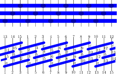
Figure 19: Time step operator and its transfer matrix representation. This construction applies to models with four site interactions where the outer two spins are control bits. These control bits are depicted as shaded circles in the figure above. An example is the folded XXZ model.

Let us now construct the single step update rule as

$$\mathcal{V}_{1}=\check{\mathcal{L}}_{1,2,3,4}(\theta)\check{\mathcal{L}}_{4,5,6,7}(\theta)\dots\check{\mathcal{L}}_{L-2,L-1,L,1}(\theta),$$ (VI.16)

where $\theta$ will be a fixed parameter of the quantum circuit. For the Floquet cycle we obtain

$$\mathcal{V}=\mathcal{V}_{3}\mathcal{V}_{2}\mathcal{V}_{1}=\mathcal{U}^{3}\times\\ \mathrm{tr}_{abc}\bigl{[}\mathcal{L}_{1,2,3,c}(\theta)\mathcal{L}_{1,2,3,b}(\theta)\mathcal{L}_{1,2,3,a}(\theta)\\ \mathcal{L}_{4,5,6,c}(\theta)\mathcal{L}_{4,5,6,b}(\theta)\mathcal{L}_{4,5,6,a}(\theta)\dots{\\ }\mathcal{L}_{L-2,L-1,L,c}(\theta)\mathcal{L}_{L-2,L-1,L,b}(\theta)\mathcal{L}_{L-2,L-1,L,a}(\theta)\bigr{]}.$$ (VI.17)

Applying the factorization formula

$$\check{R}_{123456}(\theta,0)=\check{\mathcal{L}}_{3456}(\theta)\check{\mathcal{L}}_{2345}(\theta)\check{\mathcal{L}}_{1234}(\theta)$$ (VI.18)

we can define a transfer matrix (with auxiliary space $A=(a,b,c)$)

$$t(u)=\mathrm{tr}_{A}\bigl{[}R_{(1,2,3),A}(\theta,u)R_{(4,5,6),A}(\theta,u)\dots{\\ }R_{(L-5,L-4,L-3),A}(\theta,u)R_{(L-2,L-1,L),A}(\theta,u)\bigr{]},$$ (VI.19)

which generates the time step as

$$\mathcal{V}=t^{-1}(\theta)t(0).$$ (VI.20)

These transfer matrices commute:

$$[t(u),t(v)]=0.$$ (VI.21)

With this we have established a commuting family of transfer matrices that includes the update rule of the quantum circuit at the special point $u=0$.

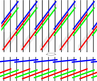
Figure 20: Transfer matrix with the operator $\check{\mathcal{G}}$.

The transfer matrix can be rewritten using the factorization (VI.1). We find

$$t(u)=\mathcal{V}_{3}\tilde{t}(u),$$ (VI.22)

where

$$\tilde{t}(u)=\\ \mathrm{tr}_{a,b,c}\bigl{[}\mathcal{G}_{1,2,a,b,c}(\theta,u)\mathcal{L}_{3,a,b,c}(-u)\mathcal{G}_{4,5,a,b,c}(\theta,u)\mathcal{L}_{6,a,b}(-u)\\ \dots\mathcal{G}_{L-2,L-1,a,b,c}(\theta,u)\mathcal{L}_{L,a,b,c}(-u)\bigr{]},$$ (VI.23)

where

$$\mathcal{G}_{1,2,3,4,5}(\theta,u)=\mathcal{P}_{1,5}\mathcal{P}_{2,5}\mathcal{P}_{3,5}\mathcal{P}_{1,4}\mathcal{P}_{2,4}\mathcal{P}_{3,4}\check{\mathcal{G}}_{1,2,3,4,5}(\theta,u).$$ (VI.24)

VII Discussion

In this paper we treated integrable spin chains with medium range interaction, focusing on cases with three-site and four site interactions. We presented a new algebraic framework which can lead to a classification of such models, and to the construction of new quantum and classical cellular automata. As it was explained in the Introduction, one of the most general problems in the field of integrability is the classification of all integrable models, and clarifying the essential features of integrability. Our results can be seen as a contribution to this multi decade endeavor. In the paper we treated the three site and four site interacting models in detail, but the generalization to longer interaction ranges is rather straightforward.

We presented partial classifications for the three site and four site spin-1/2 models, and we found a number of new models. Given the enormous literature of integrable models it is always difficult to know whether a model is indeed new; we did our best in the search of the literature and our models appear to be new. We recall that our models are translationally invariant, and in the three site interacting case they can be pictured as zig-zag spin ladders. To our best knowledge the only translationally invariant integrable three site chain the literature is the Bariev model [44]; other constructions naturally involve a staggering of some of the parameters (see for example [105, 106, 107, 108]) and thus they are not in the category of models that we are investigating.

In the family of $SU(2)$-invariant spin chains with reflection symmetry we did not find a non-trivial three site model, and we found only one new four site model given by (VI.10). In the family of $U(1)$-invariant three site chains (again with space reflection symmetry) we found two families: the Bariev model and the hard rod deformed XXZ model given by (III.52). The latter will be analyzed in detail in an upcoming publication.

A further interesting family of models is that of the IRF type Hamiltonians and quantum gates. These theories are very similar to known Restricted Solid on Solid (RSOS) models [77, 78], their Hamiltonians have the same structure, see for example [80]. However, in the case of the RSOS theories the Hilbert space is restricted (it consists of certain paths), while in our case it is simply the tensor product space of the spin chains.

For these models we also used the same formulation of our algebraic methods, as opposed to the “face weight” formulation of the Yang-Baxter relations typically used in the RSOS (or IRF) framework. However, in Section V.1 we showed that the two formulations are indeed identical in these special cases. This also implies that our models are solutions to the “face weight” formulation of the Yang-Baxter relation. We believe that the connection between the RSOS models and our new Hamiltonians deserves further study.

The family of the IRF type Hamiltonians accommodates some of the elementary cellular automata that have been studied recently [70, 76]. We found that out of the classical cellular automata treated in [76] the Rule150 and Rule105 models are Yang-Baxter integrable, and they can be deformed into quantum cellular automata. We also gave a recipe for computing extensive local charges for these quantum and classical cellular automata, and we derived the concrete formulas for the first charge of the Rule150 and Rule105 models. Putting everything together, our construction can be seen as a remarkable link between classical and quantum integrable models.

In contrast, we did not find such three site structures for the famous Rule54 model. We pointed out that the construction of [76] does not yield new conserved charges on top of the known ones, and the transfer matrices derived there are functionally dependent on the known charges. Thus the problem of the integrability of the Rule54 model is still open. A very important piece of the puzzle was presented in [74], where a six site interacting Hamiltonian was constructed, which commutes with the Floquet update rule of the Rule54 model. This suggest that the model could lie in the family of six site interacting models. Preliminary computations show that this is indeed the case: we found a new local extensive charge with interaction range $\ell=10$ using the proper generalization of our methods. We will present this result in a future work.

It would be interesting to continue the partial classification of medium range models, extending our results to more complicated three site or four site interacting cases or to higher dimensional local spaces. In both cases a much larges parameter space opens up, and a clear physical motivation is needed to formulate the restrictions for the Hamiltonians. Symmetries can be chosen as guiding principles, together with special assumptions on the structure of the Hamiltonian. A known four site interacting model is the folded XXZ model treated in [52, 53, 54]. This Hamiltonian has a particular structure: it has two control bits and two action bits, and its algebraic treatment leads to a Yang-Baxter integrable classical cellular automaton (see [81] and Section VI.1). It would be interesting to classify models with a similar structure, potentially leading to new cellular automata with four site update rules.

An other interesting question is whether our constructions exhaust all possibilities for integrable quantum circuits. The IRF type circuits show very clearly that if the Lax operators have a special structure, then this allows the construction of special brickwork circuits, which would be meaningless for other types of Lax operators. Therefore it can not be excluded, that some other sorts of special circuits can be built if we impose some other special structure on the building blocks.

In this regard let us return to the so-called box-ball systems mentioned in the Introduction [82, 83]. These are classical cellular automata with a less local update procedure, which is performed by acting with a certain transfer matrix which does not factorize into commuting local unitary operators. Theses systems are special cases of so-called filter automata [84, 85, 86, 87]. The crucial ingredient of such a construction is a Lax operator which becomes deterministic at some special points, but the regularity condition (that would lead to strictly local update rules) is not required. Our solutions for the integrable Lax operators could also be used to construct such filter automata.

In this paper we discussed the physical properties of our models only in passing. We explained that the bond-site transformed XYZ model of Section V.2 describes interacting dynamics of Domain Walls, with or without Domain Wall number conservation. And we will publish a paper dealing specifically with the hard rod deformed XXZ model found in Section III.4. We believe that the other new spin chain and quantum gate models also deserve further attention.

Finally let us mention that our methods could be relevant for also the AdS/CFT conjecture. It is known that in the planar limit the dilatation operator of the gauge theory is essentially an integrable Hamiltonian with long range interaction [109, 110]. The spectrum of this Hamiltonian is now understood using the so-called quantum spectral curve method [111, 112, 113], but there is no clear understanding of the actual Hamiltonian on the operator level. It is known that it is a long range deformation of an integrable nearest neighbor chain, but it is not clear how to perform the long range deformation in a finite volume [114]. Our methods could give a recipe for this problem: perhaps there is a truncation scheme where we could gradually increase the interaction range of the chains while still using our present methods at each step. This appears to be a promising direction for future work.

Appendix A Counter-example to the original conjecture of [33]

Here we discuss a counter-example to the original conjecture of [33] regarding the integrability of nearest neighbor spin chains. In [33] it was claimed that a sufficient condition of integrability is the existence of a three-site charge which commutes with the Hamiltonian. However, it was not stressed in [33] that the Hamiltonian has to be dynamical.

For example consider the family of models defined by the two charges

$$\begin{split}Q_{2}&=\sum_{j}\sigma^{z}_{j}\sigma^{z}_{j+1},\\ Q_{3}&=\sum_{j}(1-\sigma^{z}_{j}\sigma^{z}_{j+2})(\sigma^{x}_{j+1}+\kappa\sigma^{z}_{j+1}).\end{split}$$ (A.1)

Here $\kappa\in\mathbb{R}$ is a coupling constant. Direct computation shows that $[Q_{3},Q_{2}]=0$ for every $\kappa$. The model is integrable for $\kappa=0$, it is a special point of the bond-site transformed XYZ model considered in Section V.2. However, a non-zero $\kappa$ introduces a term which our classification found to be non-integrable. To confirm that the model is indeed non-integrable, we investigated the level spacing distribution for $\kappa=1$ and confirmed the Wigner-Dyson statistics characteristic for chaotic models. This computation was performed by Dávid Szász-Schagrin and we are thankful to him.

This example shows, that if the nearest neighbor charge $Q_{2}$ is not dynamical, then the existence of a commuting charge $Q_{3}$ is not enough to ensure integrability of the model.

Appendix B Bond-site transformation

A number of models that we encountered in this work together with the folded XXZ model treated in [52, 53, 54] allow for an alternative description after performing a bond-site transformation. This is a non-local transformation, and in the models of interest it leads to Hamiltonians with shorter interaction range. The bond-site transformation is a special case of the more general Clifford transformations treated recently in [56]; here we just treat this simple case.

The first observation is that in some models the dynamical Hamiltonian (be it a three-site or four-site operator) commutes with the non-dynamical charge

$$Q_{2}=\sum_{j}\frac{1-\sigma^{z}_{j}\sigma^{z}_{j+1}}{2}.$$ (B.1)

Here we chose the conventions such that $Q_{2}$ has zero eigenvalue on ferromagnetic states in the computational basis. Then the non-zero contributions to $Q_{2}$ originate from nearest neighbors where the two spins are different. Such a situation can be interpreted as a Domain Wall (DW), and then $Q_{2}$ is seen as the total DW number which is conserved. It is then natural to expect that the Hamiltonian can be interpreted as an operator that generates dynamics for the DW’s.

This is seen explicitly by performing a bond-site transformation, either in finite volume with open boundary conditions, or directly in infinite volume. The idea is to put spin-1/2 variables on the bonds between lattice sites, and to perform a change of basis starting from the original computational basis. For each bond we write down a $\circ$ (up spin) if the two neighboring spins are identical, and a $\bullet$ (down spin) if they are different. This is a highly non-local transformation, which can be inverted (up to simple complications at the boundaries). Then we also obtain a new Hamiltonian in the new basis.

Such a transformation can be performed for any spin chain with interaction range $\ell$. The new Hamiltonian will be local if the original one respects spin reflection invariance. Nevertheless, the new interaction will generally have range $\ell+1$ in the bond picture. It is important that the bond-site transformation can be performed even if $Q_{2}$ is not conserved: in this case Domain Walls can be created or annihilated. The only requirement for the locality of the transformation is the spin-flip invariance in a given basis.

The utility of the transformation shows itself if the new model has a smaller interaction range. A range of $\ell-1$ can be obtained if a further special condition holds: The original Hamiltonian density should be such that it does not change the spins at the first and the last sites of its support. Then only the bonds within the support of length $\ell$ are modified, which means that in the bond basis the interaction range will be $\ell-1$.

A concrete example for the site-bond transformation was presented in [54] in the case of the folded XXZ model. There the first few charges are given by (II.8). The charge $Q_{4}$ indeed preserves the first and last spins, and the domain wall number given by $Q_{2}$ is also conserved. After the bond-site transformation the charge $Q_{4}$ becomes identical to the three-site Hamiltonian (III.52) with $\Delta=0$, which is interpreted as the hard rod deformation of the XX model.

Further examples for the bond-site transformation are presented in Section (V.2). In those cases the original Hamiltonian is a three-site operator, which preserves the first and the last spins, acting non-trivially on the middle spin. In certain cases these models can be transformed into a nearest neighbor chain. In these three site interacting cases the transformation rules for a subset of the allowed operators are found to be

$$1\otimes\sigma^{x}\otimes 1 \leftrightarrow\sigma^{x}\otimes\sigma^{x},$$ (B.2)

$$-\sigma^{z}\otimes\sigma^{x}\otimes\sigma^{z} \leftrightarrow\sigma^{y}\otimes\sigma^{y},$$ (B.3)

$$\sigma^{z}\otimes 1\otimes\sigma^{z} \leftrightarrow\sigma^{z}\otimes\sigma^{z},$$ (B.4)

$$\sigma^{z}\otimes\sigma^{y}\otimes 1 \leftrightarrow\sigma^{y}\otimes\sigma^{x},$$ (B.5)

$$1\otimes\sigma^{y}\otimes\sigma^{z} \leftrightarrow\sigma^{x}\otimes\sigma^{y}.$$ (B.6)

On the l.h.s. above we listed the three site interacting operators allowed by the requirements, which are transformed into the two site operators on the r.h.s.

Appendix C Inversion relation for the $R$-matrices

Here we show that the regularity property (III.5) of the $R$-matrix and its inversion relation (III.6) are not independent properties.

Substituting $\lambda_{1}=\lambda_{3}$ to the $YB$ equation (III.4) we get

$$R_{12}(\lambda_{1},\lambda_{2})R_{13}(\lambda_{1},\lambda_{1})R_{23}(\lambda_{2},\lambda_{1})=\\ =R_{23}(\lambda_{2},\lambda_{1})R_{13}(\lambda_{1},\lambda_{1})R_{12}(\lambda_{1},\lambda_{2}).$$ (C.1)

Using the regularity property (III.5) we obtain that

$$R_{12}(\lambda_{1},\lambda_{2})R_{21}(\lambda_{2},\lambda_{1})=\\ =R_{23}(\lambda_{2},\lambda_{1})R_{32}(\lambda_{1},\lambda_{2}).$$ (C.2)

We can see that the left and the right hand sides act trivially on $3$ and $1$ spaces, respectively. Therefore they have to be equal to an operator $X_{2}$ acting only on the second space. Writing out the rapidity dependence we get

$$R_{12}(\lambda_{1},\lambda_{2})R_{21}(\lambda_{2},\lambda_{1}) =X_{2}(\lambda_{1},\lambda_{2})$$ (C.3)

$$R_{23}(\lambda_{2},\lambda_{1})R_{32}(\lambda_{1},\lambda_{2}) =X_{2}(\lambda_{1},\lambda_{2}).$$ (C.4)

The second equation can be rewritten as

$$R_{12}(\lambda_{2},\lambda_{1})R_{21}(\lambda_{1},\lambda_{2})=X_{1}(\lambda_{1},\lambda_{2}).$$ (C.5)

Substituting back to (C.3) we obtain that

$$X_{1}(\lambda_{2},\lambda_{1})=X_{2}(\lambda_{1},\lambda_{2}).$$ (C.6)

Since the l.h.s. and the r.h.s. act on different spaces the operator $X$ should be proportional to the identity, i.e.

$$R_{12}(\lambda,\mu)R_{21}(\mu,\lambda)\sim 1.$$ (C.7)

Appendix D Factorization property of the $R$-matrix

Here we prove Theorem 1.

Substitute $v=0$ to the $RLL$ relation we get

$$R_{A,(12)}(u,0)\mathcal{L}_{A,3}(u)\mathcal{L}_{(12),3}(0)=\\ \mathcal{L}_{(12),3}(0)\mathcal{L}_{A,3}(u)R_{A,(12)}(u,0).$$ (D.1)

Now let us use the regularity of the Lax operator to obtain

$$R_{A,(12)}(u,0)\mathcal{L}_{A,3}(u)=\mathcal{L}_{A,2}(u)\tilde{R}_{A,(31)}(u,0).$$ (D.2)

After a simple rearrangement we get

$$\mathcal{L}_{A,2}(u)^{-1}R_{A,(12)}(u,0)=R_{A,(31)}(u,0)\mathcal{L}_{A,3}(u)^{-1}.$$ (D.3)

We can see that the l.h.s. and the r.h.s. act trivially on the spaces $3$ and $2$, respectively, therefore they have to be equal to an operator that acts only on space $1$:

$$\mathcal{L}_{A,2}(u)^{-1}R_{A,(12)}(u,0) =X_{A,1}(u),$$ (D.4)

$$R_{A,(31)}(u,0)\mathcal{L}_{A,3}(u)^{-1} =X_{A,1}(u).$$ (D.5)

The second equation can be written as

$$R_{A,(12)}(u,0)=X_{A,2}\mathcal{L}_{A,1}(u).$$ (D.6)

Substituting back to (D.4) we obtain that

$$X_{A,2}(u)\mathcal{L}_{A,1}(u)=\mathcal{L}_{A,2}(u)X_{A,1}(u),$$ (D.7)

therefore

$$\mathcal{L}_{A,2}(u)^{-1}X_{A,2}(u)=X_{A,1}(u)\mathcal{L}_{A,1}(u)^{-1}.$$ (D.8)

Since the l.h.s. and the r.h.s. act trivially on spaces $1$ and $2$ they have to be equal to an operator acting only on the auxiliary space $A$:

$$\mathcal{L}_{A,2}(u)^{-1}X_{A,2}(u) =Y_{A}(u),$$ (D.9)

$$X_{A,1}(u)\mathcal{L}_{A,1}(u)^{-1} =Y_{A}(u).$$ (D.10)

From the first equation we obtain

$$X_{A,1}(u)=\mathcal{L}_{A,1}(u)Y_{A}(u).$$ (D.11)

Substituting back to (D.10) we obtain that

$$[\mathcal{L}_{A,1}(u),Y_{A}(u)]=0.$$ (D.12)

Substituting back to (D.6) the $R$-matrix reads as

$$R_{A,(12)}(u,0)=\mathcal{L}_{A,2}(u)\mathcal{L}_{A,1}(u)Y_{A}(u).$$ (D.13)

We are almost ready. The only remaining thing is to prove that the operator $Y_{A}(u)$ has to proportional to the identity.

We also know that the $R$-matrix is regular i.e.

$$R_{A,(12)}(0,0)=P_{A,(12)},$$ (D.14)

therefore

$$Y_{A}(0)\sim 1.$$ (D.15)

Let us substitute $\lambda_{1}=u$, $\lambda_{2}=v$ and $\lambda_{3}=0$ to the YB equation.

$$R_{A,B}(u,v)R_{A,(12)}(u,0)R_{B,(12)}(v,0)=\\ R_{B,(12)}(v,0)R_{A,(12)}(u,0)R_{A,B}(u,v).$$ (D.16)

Using (D.13) we obtain that

$$R_{A,B}(u,v)\mathcal{L}_{A,2}(u)\mathcal{L}_{B,2}(v)\mathcal{L}_{A,1}(u)\mathcal{L}_{B,1}(v)Y_{A}(u)Y_{B}(v)=\\ \mathcal{L}_{B,2}(v)\mathcal{L}_{A,2}(u)\mathcal{L}_{B,1}(v)\mathcal{L}_{A,1}(u)Y_{A}(u)Y_{B}(v)R_{A,B}(u,v).$$ (D.17)

Using the RLL relation on the l.h.s. we obtain that

$$R_{A,B}(u,v)\mathcal{L}_{A,2}(u)\mathcal{L}_{B,2}(v)\mathcal{L}_{A,1}(u)\mathcal{L}_{B,1}(v)Y_{A}(u)Y_{B}(v)=\\ \mathcal{L}_{B,2}(v)\mathcal{L}_{A,2}(u)\mathcal{L}_{B,1}(v)\mathcal{L}_{A,1}(u)R_{A,B}(u,v)Y_{A}(u)Y_{B}(v).$$ (D.18)

Substituting back to (D.17) we obtain that

$$[R_{A,B}(u,v),Y_{A}(u)Y_{B}(v)]=0.$$ (D.19)

The operator $Y_{A}(u)$ can only be non-trivial if the $R$-matrix has gauge symmetry (spectral parameter dependent symmetry).We assumed that such symmetry is excluded therefore

$$Y_{A}(u)=Y_{A}$$ (D.20)

Using the equation (D.15) we can see that the operator $Y_{A}$ has to proportional to the identity.

References

- Bethe [1931] H. Bethe, Zur theorie der metalle, Zeitschrift für Physik A71, 205 (1931).
- Onsager [1944] L. Onsager, Crystal statistics. i. a two-dimensional model with an order-disorder transition, Phys. Rev. 65, 117 (1944).
- Yang [1967] C. N. Yang, Some exact results for the many-body problem in one dimension with repulsive delta-function interaction, Phys. Rev. Lett. 19, 1312 (1967).
- Baxter [1982] R. J. Baxter, Exactly solved models in statistical mechanics (London: Academic Press Inc, 1982).
- Faddeev [1995] L. Faddeev, Instructive history of the quantum inverse scattering method, Acta Appl. Math. 39, 69 (1995).
- Lieb and Liniger [1963] E. H. Lieb and W. Liniger, Exact analysis of an interacting bose gas. i. the general solution and the ground state, Phys. Rev. 130, 1605 (1963).
- Mussardo [1992] G. Mussardo, Off-critical statistical models: Factorized scattering theories and bootstrap program, Phys. Rept. 218, 215 (1992).
- Caux and Mossel [2011] J.-S. Caux and J. Mossel, Remarks on the notion of quantum integrability, J. Stat. Mech. 2011, 02023 (2011), arXiv:1012.3587 [cond-mat.str-el] .
- Faddeev [1996] L. D. Faddeev, How Algebraic Bethe Ansatz works for integrable model, arXiv e-prints (1996), arXiv:hep-th/9605187 [hep-th] .
- Haldane [1988] F. D. M. Haldane, Exact jastrow-gutzwiller resonating-valence-bond ground state of the spin- antiferromagnetic heisenberg chain with 1/ exchange, Phys. Rev. Lett. 60, 635 (1988).
- Shastry [1988] B. S. Shastry, Exact solution of an s=1/2 heisenberg antiferromagnetic chain with long-ranged interactions, Phys. Rev. Lett. 60, 639 (1988).
- Inozemtsev [1990] V. I. Inozemtsev, On the connection between the one-dimensional s=1/2 heisenberg chain and haldane-shastry model, J. Stat. Phys. 59, 1143 (1990).
- Essler et al. [2005] F. H. L. Essler, H. Frahm, F. Göhmann, A. Klümper, and V. E. Korepin, The One-Dimensional Hubbard Model (Cambridge University Press, Cambridge, 2005).
- Talstra and Haldane [1995] J. C. Talstra and F. D. M. Haldane, Integrals of motion of the haldane-shastry model, J. Phys. A 28, 2369–2377 (1995), arXiv:cond-mat/9411065 [cond-mat] .
- Bernard et al. [1993] D. Bernard, M. Gaudin, F. D. M. Haldane, and V. Pasquier, Yang-Baxter equation in spin chains with long range interactions, arXiv e-prints (1993), arXiv:hep-th/9301084 [cond-mat] .
- Inozemtsev [2003] V. I. Inozemtsev, Integrable Heisenberg-van Vleck chains with variable range exchange, Phys. Part. Nucl. 34, 166 (2003), arXiv:hep-th/0201001 .
- Kulish and Sklyanin [1982] P. Kulish and E. Sklyanin, Solutions of the yang-baxter equation., J. Sov. Math. 19, 1596 (1982).
- Kulish et al. [1981] P. P. Kulish, N. Y. Reshetikhin, and E. K. Sklyanin, Yang-baxter equation and representation theory: I, Lett. Math. Phys. 5, 393 (1981).
- Jimbo [1985] M. Jimbo, A q difference analog of U(g) and the Yang-Baxter equation, Lett. Math. Phys. 10, 63 (1985).
- Kennedy [1992] T. Kennedy, Solutions of the Yang-Baxter equation for isotropic quantum spin chains, J. Phys. A 25, 2809 (1992).
- Mutter and Schmitt [1995] K.-H. Mutter and A. Schmitt, Solvable spin-1 models in one dimension, J. Phys. A 28, 2265 (1995).
- Sogo et al. [1982] K. Sogo, M. Uchinami, Y. Akutsu, and M. Wadati, Classification of Exactly Solvable Two-Component Models, Prog. Theor. Phys. 68, 508 (1982).
- Hietarinta [1993] J. Hietarinta, Solving the two-dimensional constant quantum Yang-Baxter equation, J. Math. Phys. 34, 1725 (1993).
- Khachatryan and Sedrakyan [2013] S. Khachatryan and A. Sedrakyan, On the Solutions of the Yang-Baxter Equations with General Inhomogeneous Eight-Vertex R-Matrix: Relations with Zamolodchikov’s Tetrahedral Algebra, J. Stat. Phys. 150, 130 (2013), arXiv:1208.4339 [math-ph] .
- Dye [2003] H. A. Dye, Unitary Solutions to the Yang-Baxter Equation in Dimension Four, Quant. Inf. Proc. 2, 117 (2003), arXiv:quant-ph/0211050 [quant-ph] .
- Pourkia [2018] A. Pourkia, Solutions to the constant Yang-Baxter equation in all dimensions, arXiv e-prints (2018), arXiv:1806.08400 [quant-ph] .
- Vieira [2018] R. S. Vieira, Solving and classifying the solutions of the Yang-Baxter equation through a differential approach. Two-state systems, JHEP 10, 110, arXiv:1712.02341 [nlin.SI] .
- de Leeuw et al. [2019] M. de Leeuw, A. Pribytok, and P. Ryan, Classifying two-dimensional integrable spin chains, J. Phys. A 52, 505201 (2019), arXiv:1904.12005 [math-ph] .
- de Leeuw et al. [2020a] M. de Leeuw, C. Paletta, A. Pribytok, A. L. Retore, and P. Ryan, Classifying Nearest-Neighbor Interactions and Deformations of AdS, Phys. Rev. Lett. 125, 031604 (2020a), arXiv:2003.04332 [hep-th] .
- de Leeuw et al. [2020b] M. de Leeuw, A. Pribytok, A. L. Retore, and P. Ryan, New integrable 1D models of superconductivity, J. Phys. A 53, 385201 (2020b), arXiv:1911.01439 [math-ph] .
- de Leeuw et al. [2020c] M. de Leeuw, C. Paletta, A. Pribytok, A. L. Retore, and P. Ryan, Yang-Baxter and the Boost: splitting the difference, arXiv e-prints (2020c), arXiv:2010.11231 [math-ph] .
- de Leeuw et al. [2021] M. de Leeuw, C. Paletta, and B. Pozsgay, Constructing Integrable Lindblad Superoperators, Phys. Rev. Lett. 126, 240403 (2021), arXiv:2101.08279 [cond-mat.stat-mech] .
- Grabowski and Mathieu [1995] M. P. Grabowski and P. Mathieu, Integrability test for spin chains, J. Phys. A 28, 4777 (1995), arXiv:hep-th/9412039 [hep-th] .
- Klümper and Sakai [2002] A. Klümper and K. Sakai, The thermal conductivity of the spin- 1/2 XXZ chain at arbitrary temperature, J. Phys. A 35, 2173 (2002), arXiv:cond-mat/0112444 .
- Alcaraz and Bariev [1999a] F. C. Alcaraz and R. Z. Bariev, An Exactly Solvable Constrained XXZ Chain, arXiv e-prints (1999a), arXiv:cond-mat/9904042 [cond-mat.stat-mech] .
- Alcaraz and Bariev [1999b] F. C. Alcaraz and R. Z. Bariev, Integrable models of strongly correlated particles with correlated hopping, Phys. Rev. B 59, 3373 (1999b), arXiv:cond-mat/9904129 [cond-mat.stat-mech] .
- Alcaraz and Bariev [1999c] F. C. Alcaraz and R. Z. Bariev, Exact solution of the asymmetric exclusion model with particles of arbitrary size, Phys. Rev. E 60, 79 (1999c), arXiv:cond-mat/9904130 [cond-mat.stat-mech] .
- Karnaukhov and Ovchinnikov [2002] I. N. Karnaukhov and A. A. Ovchinnikov, One-dimensional strongly interacting Luttinger liquid of lattice spinless fermions, Europhys. Lett. 57, 540 (2002), arXiv:cond-mat/0110289 [cond-mat.str-el] .
- Alcaraz and Lazo [2007] F. C. Alcaraz and M. J. Lazo, Exactly solvable interacting vertex models, J. Stat. Mech. 2007, 08008 (2007), arXiv:0706.2178 [cond-mat.stat-mech] .
- Abarenkova and Pronko [2002] N. Abarenkova and A. Pronko, Temperature correlation function in the absolutely anisotropic xxz heisenberg magnet, Theor. Math. Phys. 131, 690–703 (2002).
- Trippe et al. [2010] C. Trippe, F. Göhmann, and A. Klümper, Thermodynamics and short-range correlations of the XXZ chain close to its triple point, J. Stat. Mech. 2010, 01021 (2010), arXiv:0912.1739 [cond-mat.stat-mech] .
- Fendley et al. [2003a] P. Fendley, K. Schoutens, and J. de Boer, Lattice Models with N=2 Supersymmetry, Phys. Rev. Lett. 90, 120402 (2003a), arXiv:hep-th/0210161 [hep-th] .
- Fendley et al. [2003b] P. Fendley, B. Nienhuis, and K. Schoutens, Lattice fermion models with supersymmetry, J. Phys. A 36, 12399 (2003b), arXiv:cond-mat/0307338 [cond-mat.str-el] .
- Bariev [1991] R. Z. Bariev, Integrable spin chain with two- and three-particle interactions, J. Phys. A 24, L549 (1991).
- Zhou [1996] H.-Q. Zhou, Quantum integrability for the one-dimensional Bariev chain, Phys. Lett. A 221, 104 (1996).
- Shiroishi and Wadati [1997] M. Shiroishi and M. Wadati, Integrability of the one-dimensional bariev model, J. Phys. A 30, 1115 (1997).
- Fendley [2019] P. Fendley, Free fermions in disguise, Journal of Physics A Mathematical General 52, 335002 (2019), arXiv:1901.08078 [cond-mat.stat-mech] .
- Alcaraz and Pimenta [2020a] F. C. Alcaraz and R. A. Pimenta, Free fermionic and parafermionic quantum spin chains with multispin interactions, Phys. Rev. B 102, 121101 (2020a), arXiv:2005.14622 [cond-mat.stat-mech] .
- Alcaraz and Pimenta [2020b] F. C. Alcaraz and R. A. Pimenta, Integrable quantum spin chains with free fermionic and parafermionic spectrum, arXiv e-prints (2020b), arXiv:2010.01116 [cond-mat.stat-mech] .
- Alcaraz and Pimenta [2021] F. C. Alcaraz and R. A. Pimenta, Free parafermionic Z(N) and free fermionic XY quantum chains, arXiv e-prints (2021), arXiv:2108.04372 [cond-mat.stat-mech] .
- Elman et al. [2020] S. J. Elman, A. Chapman, and S. T. Flammia, Free fermions behind the disguise, arXiv e-prints (2020), arXiv:2012.07857 [quant-ph] .
- Zadnik and Fagotti [2021] L. Zadnik and M. Fagotti, The Folded Spin-1/2 XXZ Model: I. Diagonalisation, Jamming, and Ground State Properties, SciPost Phys. Core 4, 10 (2021), arXiv:2009.04995 [cond-mat.stat-mech] .
- Zadnik et al. [2021] L. Zadnik, K. Bidzhiev, and M. Fagotti, The Folded Spin-1/2 XXZ model: II. Thermodynamics and hydrodynamics with a minimal set of charges, SciPost Phys. 10, 99 (2021), arXiv:2011.01159 [cond-mat.stat-mech] .
- Pozsgay et al. [2021] B. Pozsgay, T. Gombor, A. Hutsalyuk, Y. Jiang, L. Pristyák, and E. Vernier, An integrable spin chain with Hilbert space fragmentation and solvable real time dynamics, arXiv e-prints (2021), arXiv:2105.02252 [cond-mat.stat-mech] .
- Bidzhiev et al. [2021] K. Bidzhiev, M. Fagotti, and L. Zadnik, Macroscopic effects of localised measurements in jammed states of quantum spin chains, arXiv e-prints (2021), arXiv:2108.03230 [cond-mat.stat-mech] .
- Jones and Linden [2021] N. G. Jones and N. Linden, Integrable spin chains and the Clifford group, arXiv e-prints (2021), arXiv:2107.02184 [math-ph] .
- Chandran and Laumann [2015] A. Chandran and C. R. Laumann, Semiclassical limit for the many-body localization transition, Phys. Rev. B 92, 024301 (2015), arXiv:1501.01971 [cond-mat.dis-nn] .
- Nahum et al. [2017] A. Nahum, J. Ruhman, S. Vijay, and J. Haah, Quantum Entanglement Growth under Random Unitary Dynamics, Phys. Rev. X 7, 031016 (2017), arXiv:1608.06950 [cond-mat.stat-mech] .
- Nahum et al. [2018] A. Nahum, S. Vijay, and J. Haah, Operator Spreading in Random Unitary Circuits, Phys. Rev. X 8, 021014 (2018), arXiv:1705.08975 [cond-mat.str-el] .
- von Keyserlingk et al. [2018] C. W. von Keyserlingk, T. Rakovszky, F. Pollmann, and S. L. Sondhi, Operator Hydrodynamics, OTOCs, and Entanglement Growth in Systems without Conservation Laws, Phys. Rev. X 8, 021013 (2018), arXiv:1705.08910 [cond-mat.str-el] .
- Rakovszky et al. [2018] T. Rakovszky, F. Pollmann, and C. W. von Keyserlingk, Diffusive Hydrodynamics of Out-of-Time-Ordered Correlators with Charge Conservation, Phys. Rev. X 8, 031058 (2018), arXiv:1710.09827 [cond-mat.stat-mech] .
- Khemani et al. [2018] V. Khemani, A. Vishwanath, and D. A. Huse, Operator Spreading and the Emergence of Dissipative Hydrodynamics under Unitary Evolution with Conservation Laws, Phys. Rev. X 8, 031057 (2018), arXiv:1710.09835 [cond-mat.stat-mech] .
- Chan et al. [2018] A. Chan, A. De Luca, and J. T. Chalker, Solution of a Minimal Model for Many-Body Quantum Chaos, Phys. Rev. X 8, 041019 (2018), arXiv:1712.06836 [cond-mat.stat-mech] .
- Vanicat et al. [2018] M. Vanicat, L. Zadnik, and T. Prosen, Integrable Trotterization: Local Conservation Laws and Boundary Driving, Phys. Rev. Lett. 121, 030606 (2018), arXiv:1712.00431 [cond-mat.stat-mech] .
- Destri and De Vega [1987] C. Destri and H. De Vega, Light-cone lattice approach to fermionic theories in 2d: The massive thirring model, Nucl. Phys. B 290, 363 (1987).
- Volkov [1992] A. Y. Volkov, Quantum Volterra model, Phys. Lett. A 167, 345 (1992).
- Faddeev and Volkov [1994] L. D. Faddeev and A. Y. Volkov, Hirota equation as an example of integrable symplectic map, Lett. Math. Phys. 32, 125 (1994), arXiv:hep-th/9405087 .
- Sá et al. [2021] L. Sá, P. Ribeiro, and T. Prosen, Integrable Non-unitary Open Quantum Circuits, Phys. Rev. B 103, 115132 (2021), arXiv:2011.06565 [cond-mat.stat-mech] .
- Bobenko et al. [1993] A. Bobenko, M. Bordemann, C. Gunn, and U. Pinkall, On two integrable cellular automata, Comm. Math. Phys. 158, 127 (1993).
- Buča et al. [2021] B. Buča, K. Klobas, and T. Prosen, Rule 54: Exactly solvable model of nonequilibrium statistical mechanics, J. Stat. Mech. 2021, 074001 (2021), arXiv:2103.16543 [cond-mat.stat-mech] .
- Klobas et al. [2021] K. Klobas, B. Bertini, and L. Piroli, Exact thermalization dynamics in the “rule 54” quantum cellular automaton, Phys. Rev. Lett. 126, 160602 (2021), arXiv:2012.12256 [cond-mat.stat-mech] .
- Klobas and Bertini [2021] K. Klobas and B. Bertini, Exact relaxation to Gibbs and non-equilibrium steady states in the quantum cellular automaton Rule 54, arXiv e-prints (2021), arXiv:2104.04511 [cond-mat.stat-mech] .
- Klobas and Bertini [2021] K. Klobas and B. Bertini, Entanglement dynamics in Rule 54: exact results and quasiparticle picture, arXiv e-prints (2021), arXiv:2104.04513 [cond-mat.stat-mech] .
- Friedman et al. [2019] A. J. Friedman, S. Gopalakrishnan, and R. Vasseur, Integrable many-body quantum floquet-thouless pumps, Phys. Rev. Lett. 123, 170603 (2019), arXiv:1905.03265 [cond-mat.stat-mech] .
- Gopalakrishnan [2018] S. Gopalakrishnan, Operator growth and eigenstate entanglement in an interacting integrable Floquet system, Phys. Rev. B 98, 060302 (2018), arXiv:1806.04156 [cond-mat.stat-mech] .
- Prosen [2021] T. Prosen, Reversible Cellular Automata as Integrable Interactions Round-a-Face: Deterministic, Stochastic, and Quantized, arXiv e-prints (2021), arXiv:2106.01292 [cond-mat.stat-mech] .
- Andrews et al. [1984] G. E. Andrews, R. J. Baxter, and P. J. Forrester, Eight-vertex sos model and generalized rogers-ramanujan-type identities, J. Stat. Phys. 35, 193 (1984).
- Baxter and Forrester [1985] R. J. Baxter and P. J. Forrester, Further exact solutions of the eight-vertex sos model and generalizations of the rogers-ramanujan identities, J. Stat. Phys. 38, 435 (1985).
- Pasquier [1988] V. Pasquier, Etiology of IRF models, Comm. Math. Phys. 118, 355 (1988).
- Bianchini et al. [2015] D. Bianchini, E. Ercolessi, P. A. Pearce, and F. Ravanini, Rsos quantum chains associated with off-critical minimal models and parafermions, J. Stat. Mech. 2015, 03010 (2015), arXiv:1412.4942 [hep-th] .
- Pozsgay [2021] B. Pozsgay, A Yang-Baxter integrable cellular automaton with a four site update rule, J. Phys. A 10.1088/1751-8121/ac1dbf (2021), arXiv:2106.00696 [cond-mat.stat-mech] .
- Takahashi and Satsuma [1990] D. Takahashi and J. Satsuma, A soliton cellular automaton, J. Phys. Soc. Jap. 59, 3514 (1990).
- Inoue et al. [2012] R. Inoue, A. Kuniba, and T. Takagi, Integrable structure of box-ball systems: crystal, Bethe ansatz, ultradiscretization and tropical geometry, J. Phys. A 45, 073001 (2012), arXiv:1109.5349 [math-ph] .
- Park et al. [1986] J. K. Park, K. Steiglitz, and W. P. Thurston, Soliton-like behavior in automata, Phys. D 19, 423 (1986).
- Fokas et al. [1990] A. Fokas, E. Papadopoulou, and Y. Saridakis, Soliton cellular automata, Phys. D 41, 297 (1990).
- Bruschi et al. [1992] M. Bruschi, P. Santini, and O. Ragnisco, Integrable cellular automata, Phys. Lett. A 169, 151 (1992).
- Jiang [1992] Z. Jiang, An energy-conserved solitonic cellular automaton, J. Phys. A 25, 3369 (1992).
- Kuniba et al. [2020] A. Kuniba, G. Misguich, and V. Pasquier, Generalized hydrodynamics in box-ball system, J. Phys. A 53, 404001 (2020), arXiv:2004.01569 [math-ph] .
- Ilievski et al. [2015] E. Ilievski, J. De Nardis, B. Wouters, J.-S. Caux, F. H. L. Essler, and T. Prosen, Complete Generalized Gibbs Ensembles in an Interacting Theory, Phys. Rev. Lett. 115, 157201 (2015), arXiv:1507.02993 [quant-ph] .
- Ilievski et al. [2016] E. Ilievski, M. Medenjak, T. Prosen, and L. Zadnik, Quasilocal charges in integrable lattice systems, J. Stat. Mech. 6, 064008 (2016), arXiv:1603.00440 [cond-mat.stat-mech] .
- Shiraishi [2019] N. Shiraishi, Proof of the absence of local conserved quantities in the XYZ chain with a magnetic field, Europhys. Lett. 128, 17002 (2019), arXiv:1803.02637 [cond-mat.stat-mech] .
- Fan and Wu [1969] C. Fan and F. Y. Wu, Ising model with second-neighbor interaction. i. some exact results and an approximate solution, Phys. Rev. 179, 560 (1969).
- Links et al. [2001] J. Links, H.-Q. Zhou, R. H. McKenzie, and M. D. Gould, Ladder Operator for the One-Dimensional Hubbard Model, Phys. Rev. Lett. 86, 5096 (2001), arXiv:cond-mat/0011368 [cond-mat.str-el] .
- Takesue [1987] S. Takesue, Reversible cellular automata and statistical mechanics, Phys. Rev. Lett. 59, 2499 (1987).
- Wolfram [1983] S. Wolfram, Statistical mechanics of cellular automata, Rev. Mod. Phys. 55, 601 (1983).
- Causer et al. [2020] L. Causer, I. Lesanovsky, M. C. Bañuls, and J. P. Garrahan, Dynamics and large deviation transitions of the XOR-Fredrickson-Andersen kinetically constrained model, Phys. Rev. E 102, 052132 (2020), arXiv:2006.08673 [cond-mat.stat-mech] .
- Wilkinson et al. [2020] J. W. P. Wilkinson, K. Klobas, T. Prosen, and J. P. Garrahan, Exact solution of the Floquet-PXP cellular automaton, Phys. Rev. E 102, 062107 (2020), arXiv:2006.06556 [cond-mat.stat-mech] .
- Korepin et al. [1993] V. Korepin, N. Bogoliubov, and A. Izergin, Quantum inverse scattering method and correlation functions (Cambridge University Press, 1993).
- Murakami [1998] S. Murakami, New integrable extension of the hubbard chain with variable range hopping, J. Phys. A 31, 6367–6384 (1998), arXiv:cond-mat/9802066 [cond-mat.stat-mech] .
- Delius et al. [1995] G. W. Delius, M. D. Gould, J. R. Links, and Y. Z. Zhang, Solutions of the yang-baxter equation with extra nonadditive parameters. II. uq(gl(m/n)), J. Phys. A 28, 6203 (1995).
- Verresen et al. [2019] R. Verresen, A. Vishwanath, and F. Pollmann, Stable Luttinger liquids and emergent symmetry in constrained quantum chains, arXiv e-prints (2019), arXiv:1903.09179 [cond-mat.str-el] .
- Turner et al. [2018] C. J. Turner, A. A. Michailidis, D. A. Abanin, M. Serbyn, and Z. Papić, Quantum scarred eigenstates in a Rydberg atom chain: Entanglement, breakdown of thermalization, and stability to perturbations, Phys. Rev. B 98, 155134 (2018), arXiv:1806.10933 [cond-mat.quant-gas] .
- Au-Yang and Perk [1989] H. Au-Yang and J. H. H. Perk, Onsager’s star-triangle equation: Master key to integrability, Adv. Stud. Pure Math. 19, 57 (1989).
- Pokrovsky and Bashilov [1982] S. V. Pokrovsky and Y. A. Bashilov, Star-triangle relations in the exactly solvable statistical models, Comm. Math. Phys. 84, 103 (1982).
- Popkov and Zvyagin [1993] V. Popkov and A. Zvyagin, “antichiral” exactly solvable effectively two-dimensional quantum spin model, Phys. Lett. A 175, 295 (1993).
- Frahm and Rödenbeck [1996] H. Frahm and C. Rödenbeck, Integrable models of coupled Heisenberg chains, Europhys. Lett. 33, 47 (1996), arXiv:cond-mat/9502090 [cond-mat] .
- Zvyagin [2001] A. A. Zvyagin, Bethe ansatz solvable multi-chain quantum systems, J. Phys. A 34, R21 (2001).
- Ambjorn et al. [2001] J. Ambjorn, D. Arnaudon, A. Sedrakyan, T. Sedrakyan, and P. Sorba, Integrable ladder t-J model with staggered shift of the spectral parameter, J. Phys. A 34, 5887 (2001), arXiv:hep-th/0006243 [hep-th] .
- Beisert et al. [2003] N. Beisert, C. Kristjansen, and M. Staudacher, The dilatation operator of conformal N=4 super-Yang-Mills theory, Nucl. Phys. B 664, 131 (2003), arXiv:hep-th/0303060 [hep-th] .
- Beisert [2004] N. Beisert, The Dilatation operator of N=4 super Yang-Mills theory and integrability, Phys. Rept. 405, 1 (2004), arXiv:hep-th/0407277 [hep-th] .
- Gromov et al. [2014] N. Gromov, V. Kazakov, S. Leurent, and D. Volin, Quantum Spectral Curve for Planar Super-Yang-Mills Theory, Phys. Rev. Lett. 112, 011602 (2014), arXiv:1305.1939 [hep-th] .
- Gromov et al. [2015] N. Gromov, V. Kazakov, S. Leurent, and D. Volin, Quantum spectral curve for arbitrary state/operator in AdS5/CFT4, JHEP 09, 187, arXiv:1405.4857 [hep-th] .
- Gromov [2017] N. Gromov, Introduction to the spectrum of n=4 sym and the quantum spectral curve, arXiv e-prints (2017), arXiv:1708.03648 [hep-th] .
- Bargheer et al. [2009] T. Bargheer, N. Beisert, and F. Loebbert, Long-range deformations for integrable spin chains, J. Phys. A 42, 285205 (2009), arXiv:0902.0956 [hep-th] .