The next generation: Impact of high-order analytical information on effective one body waveform models for noncircularized, spin-aligned black hole binaries.

Abstract

We explore the performance of an updated effective-one-body (EOB) model for spin-aligned coalescing black hole binaries designed to deal with any orbital configuration. The model stems from previous work involving the TEOBResumS waveform model, but incorporates recently computed analytical information up to fifth post-Newtonian (PN) order in the EOB potentials. The dynamics is then informed by Numerical Relativity (NR) quasi-circular simulations (incorporating also recently computed 4PN spin-spin and, optionally, 4.5PN spin-orbit terms). The so-constructed model(s) are then compared to various kind of NR simulations, covering either quasi-circular inspirals, eccentric inspirals and scattering configurations. For quasi-circular (534 datasets) and eccentric (28 datasets) inspirals up to coalescence, the EOB/NR unfaithfulness is well below $1\%$ except for a few outliers in the high, positive, spin corner of the parameter space, where however it does not exceed the $3\%$ level. The EOB values of the scattering angle are found to agree ($\lesssim 1\%$) with the NR predictions for most configurations, with the largest disagreement of only $\sim 4\%$ for the most relativistic one. The inclusion of some high-order analytical information in the orbital sector is useful to improve the EOB/NR agreement with respect to previous work, although the use of NR-informed functions is still crucial to accurately describe the strong-field dynamics and waveform.

I Introduction

There is an ongoing effort in building up accurate waveform model for noncircularized coalescing black-hole binaries Chiaramello and Nagar (2020); Nagar et al. (2021a); Islam et al. (2021); Nagar et al. (2021b); Albanesi et al. (2021); Liu et al. (2021); Khalil et al. (2021). In particular, the generalization of the quasicircular models TEOBResumS Nagar et al. (2020); Riemenschneider et al. (2021) to nonquasicircular configurations Chiaramello and Nagar (2020); Nagar et al. (2021a, b) has allowed the construction of the first, and currently only, effective-one-body waveform model for spin-aligned black hole binaries that is able to accurately deal with both hyperbolic captures East et al. (2013); Gold and Brügmann (2013); Nagar et al. (2021a, b) and eccentric inspirals Chiaramello and Nagar (2020); Nagar et al. (2021b) (see also Cao and Han (2017); Liu et al. (2019, 2021); Yun et al. (2021) for a different EOB-based construction limited to eccentric inspiral). In particular, the model of Ref. Chiaramello and Nagar (2020); Nagar et al. (2021b) has been used to analyze the GW source GW190521 Abbott et al. (2020a, b) under the hypothesis that it is the result of an hyperbolic capture Gamba et al. (2021). However, the most recent results of Ref. Nagar et al. (2021b) should be further improved, since the quasicircular limit of the model is considerably less accurate (EOB/NR unfaithfulness $\simeq 1\%$) than the native quasi-circular model TEOBResumS Nagar et al. (2020); Riemenschneider et al. (2021) (EOB/NR unfaithfulness $\simeq 0.1\%$). The purpose of this paper is to show that certain modifications to the underlying analytical structure of the EOB dynamics allow to do so and thus obtain a waveform model that: (i) is highly NR faithful for quasicircular coalescing BBHs; (ii) improves the EOB/NR agreement for the limited number of eccentric NR inspiral waveforms currently publicly available; (iii) it similarly allows for an improved agreement between EOB and NR scattering angles. Technically, this is accomplished using the model of Ref. Nagar et al. (2021b) where some of the analytical building blocks of the Hamiltonian are modified. In particular: (i) we implement recently computed 5PN-accurate information Bini et al. (2019, 2020) in the EOB potentials $(D,Q)$; (ii) the potentials $(A,D)$ are resummed using diagonal ($P^{3}_{3}$ for $A$) and near diagonal ($P^{3}_{2}$ for $D$) Padé approximant instead of the $P^{1}_{5}$ and $P^{0}_{3}$ approximants that have been shared by all realizations of TEOBResumS up to now. In addition, we also explore the impact of new analytical information in the spin sector. In particular, for what concerns spin-spin interaction, we incorporate all available information up to 4PN (NNLO) Levi and Steinhoff (2016a, b), following the EOB implementation of Ref. Nagar et al. (2019a). Similarly, for the spin-orbit sector we also investigate the effect of the next-to-next-to-next-to-leading order (N³LO) contribution recently obtained in Refs. Antonelli et al. (2020a, b).

The paper is organized as follows. In Sec. II we review the analytical elements of the EOB waveform model we are introducing here, in particular highlighting the differences with previous works. Section III illustrates the quasi-circular limit of the model, how it is informed by NR simulations and how it performs on the SXS waveform catalog. Similarly, Sec. IV reports EOB/NR comparisons for eccentric inspirals, while Sec. V focuses on the scattering angle. The paper is ended by concluding remarks in Sec. VI, while Appendix A presents some updates and corrections to the findings of Ref. Nagar et al. (2021b). If not otherwise specified, we use units with $c=G=1$.

II EOB dynamics with 5PN terms

II.1 The EOB potentials

The structure of the dynamics and waveform of the EOB eccentric model discussed here is the same as Ref. Nagar et al. (2021b) except for the PN accuracy of the potentials $(A,D,Q)$ and their resummed representation. Before giving details about them, let us recall the basic notation adopted. We use mass-reduced phase-space variables $(r,\varphi,p_{\varphi},p_{r_{*}})$, related to the physical ones by $r=R/M$ (relative separation), $p_{r_{*}}=P_{R_{*}}/\mu$ (radial momentum), $\varphi$ (orbital phase), $p_{\varphi}=P_{\varphi}/(\mu M)$ (angular momentum) and $t=T/M$ (time), where $\mu\equiv m_{1}m_{2}/M$ and $M\equiv m_{1}+m_{2}$. The radial momentum is $p_{r_{*}}\equiv(A/B)^{1/2}p_{r}$, where $A$ and $B$ are the EOB potentials (with included spin-spin interactions, see below Damour and Nagar (2014)) and $D=AB$ (for nonspinning systems). The EOB Hamiltonian is $\hat{H}_{\rm EOB}\equiv H_{\rm EOB}/\mu=\nu^{-1}\sqrt{1+2\nu(\hat{H}_{\rm eff}-1)}$, with $\nu\equiv\mu/M$ and $\hat{H}_{\rm eff}=\tilde{G}p_{\varphi}+\hat{H}^{\rm orb}_{\rm eff}$, where $\tilde{G}p_{\varphi}$ incorporates odd-in-spin (spin-orbit) effects while $\hat{H}^{\rm orb}_{\rm eff}$ takes into account even-in-spin effects through the use of the centrifugal radius $r_{c}$ Nagar et al. (2018), that we discuss below. The orbital Hamiltonian for non-spinning systems reads

$$\hat{H}_{\rm orb}=\sqrt{A(u)(1+p_{\varphi}u^{2})+p_{r_{*}}^{2}+Q(u,p_{r_{*}})},$$ (1)

where $u\equiv 1/r$. The Taylor expanded expressions of the $(A,D)$ potential up to 5PN accuracy read

$$A_{\rm 5PN}(u) =1-2u+2\nu\,u^{3}+\nu\left(\frac{94}{3}-\frac{41\pi^{2}}{32}\right)u^{4}+$$

$$\quad+\left[\left(\frac{2275\pi^{2}}{512}-\frac{4237}{60}+\frac{128}{5}{\gamma_{\textrm{E}}}+\frac{256}{5}\ln(2)\right)\nu+\left(\frac{41\pi^{2}}{32}-\frac{221}{6}\right)\nu^{2}+\frac{64}{5}\nu\,\ln(u)\right]u^{5}+$$

$$\quad+\nu\left[a_{6}^{c}+\left(-\frac{7004}{105}-\frac{144}{5}\nu\right)\,\ln(u)\right]u^{6},$$ (2)

$$D_{\rm 5PN}(u) =1-6\nu\,u^{2}-\left(52\nu-6\nu^{2}\right)u^{3}+$$

$$\quad+\left[\left(\frac{533}{45}+\frac{23761\pi^{2}}{1536}-\frac{1184}{15}{\gamma_{\textrm{E}}}+\frac{6496}{15}\ln(2)-\frac{2916}{5}\ln(3)\right)\nu+\left(-\frac{123\pi^{2}}{16}+296\right)\nu^{2}-\frac{592}{15}\nu\ln(u)\right]u^{4}+$$

$$\quad+\Bigg{[}\left(-\frac{294464}{175}+\frac{63707\pi^{2}}{512}+\frac{2840}{7}{\gamma_{\textrm{E}}}-\frac{120648}{35}\ln(2)+\frac{19683}{7}\ln(3)\right)\nu+$$

$$\quad\quad\quad+\left(-d_{5}^{\nu^{2}}-\frac{2216}{105}+\frac{6784}{15}{\gamma_{\textrm{E}}}+\frac{326656}{21}\ln(2)-\frac{58320}{7}\ln(3)\right)\nu^{2}+$$

$$\quad\quad\quad+\left(-\frac{1285}{3}+\frac{205\pi^{2}}{16}\right)\nu^{3}+\left(\frac{1420}{7}\nu+\frac{3392}{15}\nu^{2}\right)\ln(u)\Bigg{]}u^{5},$$ (3)

where $\gamma_{E}=0.577216\dots$ and we kept implicit the coefficient $a_{6}^{c}(\nu)$. Its analytically known expression reads Bini and Damour (2013); Damour et al. (2014a, 2015, 2016)

$$a_{\rm 6\,anlyt}^{c}(\nu)=-\frac{1066621}{1575}+\frac{246367\pi^{2}}{3072}$$

$$-\frac{14008}{105}{\gamma_{\textrm{E}}}-\frac{31736}{105}\ln(2)+\frac{243}{7}\ln(3)$$ (4)

$$+\left(\frac{64}{5}-\frac{288}{5}{\gamma_{\textrm{E}}}+\frac{928}{35}\ln(2)-\frac{972}{7}\ln(3)+a_{6}^{\nu^{2}}\right)\nu+4\nu^{2}.$$

Note that both Eq. (II.1) and (II.1) present two yet undetermined analytical coefficients, $(a_{6}^{\nu^{2}},d_{5}^{\nu^{2}})$. For simplicity, in this work we impose $d_{5}^{\nu^{2}}=0$. By contrast, following previous works, we will not use the analytical expression $a_{\rm 6\,anlyt}^{c}(\nu)$, but rather consider $a_{6}^{c}(\nu)$ as an undetermined function of $\nu$ that is informed using NR simulations. The differences between the resulting NR-informed $A$ function and the one that uses $a_{\rm 6\,anlyt}^{c}(\nu)$ will be discussed below. The $Q$ function at 5PN accuracy was obtained in Ref. Bini et al. (2020). For simplicity, here we only consider the local part of $Q$ at 5PN. Once $p_{r}$ is rewritten in terms of $p_{r_{*}}$, the function reads

$$Q_{\rm 5PNloc}(u,p_{r_{*}}) =2(4-3\nu)\nu\,u^{2}p_{r_{*}}^{4}+\left[\left(-\frac{4348}{15}+\frac{496256}{45}\ln(2)-\frac{33048}{5}\ln(3)\right)\nu-131\nu^{2}+10\nu^{3}\right]u^{3}p_{r_{*}}^{4}$$

$$\quad+\left[\left(-\frac{827}{3}-\frac{2358912}{25}\ln(2)+\frac{1399437}{50}\ln(3)+\frac{390625}{18}\ln(5)\right)\nu-\frac{27}{5}\nu^{2}+6\nu^{3}\right]u^{2}\,p_{r_{*}}^{6}+$$

$$\quad+\left[\left(-\frac{32957}{10}-\frac{28306944}{25}\ln(2)+\frac{8396622}{25}\ln(3)+\frac{781250}{3}\ln(5)\right)\nu-\frac{393}{5}\nu^{2}+188\nu^{3}-14\nu^{4}\right]u^{3}p_{r_{*}}^{6}+$$

$$\quad+\Bigg{[}\left(-\frac{6328799}{3150}-\frac{93031\pi^{2}}{1536}+\frac{3970048}{45}\ln(2)-\frac{264384}{5}\ln(3)\right)\nu+\left(-\frac{5075}{3}+\frac{31633\pi^{2}}{512}\right)\nu^{2}$$

$$\quad\quad\quad+\left(792-\frac{615\pi^{2}}{32}\right)\nu^{3}\Bigg{]}u^{4}p_{r_{*}}^{4}+\left(\frac{6}{7}\nu+\frac{18}{7}\nu^{2}+\frac{24}{7}\nu^{3}-6\nu^{4}\right)u^{2}p_{r_{*}}^{8}.$$ (5)

Here we will keep the function $Q$ in its PN-expanded form. By contrast, both the $(A,D)$ functions will be resummed using Padé approximants, although with different choices with respect to previous work. Within the TEOBResumS models, the formal 5PN-accurate $A$ function is always resummed via a $(1,5)$ Padé approximant. As we will illustrate below, this approximant develops a spurious pole when $a_{6}^{c}=a_{\rm 6anlyt}^{c}$. Since we also want to get a handle on the performance of the pure analytical information, we are forced to change the resummation choice. To do so, we follow the most straightforward approach and use the diagonal Padé approximant, that is

$$A(u,\nu;a_{6}^{c})=P^{3}_{3}[A_{\rm 5PN}(u,\nu;a_{6}^{c})],$$ (6)

where it is intended that the $\ln(u)$ terms are treated as numerical constants when computing the Padé.

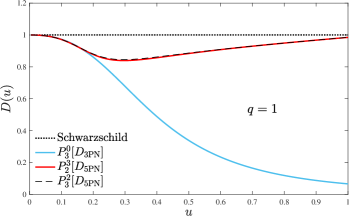
Figure 1: Comparison between different realizations of the $D$ function for $q=1$: the $P^{0}_{3}[D_{\rm 3PN}]$ used in the standard implementation of TEOBResumS (blue online). Since the $P^{0}_{5}[D_{\rm 5PN}]$ develops a spurious pole for $0<u<1$, we plot instead $P^{3}_{2}[D_{\rm 5PN}]$ and $P^{2}_{3}[D_{\rm 5PN}]$, that are almost identical. However, the latter develops a spurious pole well outside the domain (around $u\sim 8$). Note that both approximants are quantitatively consistent with the Schwarzschild potential, $D=1$ (dotted line). We choose the $P^{3}_{2}[D_{\rm 5PN}]$ Padé approximant to represent the $D$ function.

The 3PN-accurate $D$ function, that in TEOBResumS, is resummed using a $(0,3)$ approximant. When the same is attempted with the 5PN-accurate function (with $d_{5}^{\nu^{2}}=0$), spurious poles again show up for any value of $\nu$. By contrast, the quasi-diagonal Padé approximants $P^{3}_{2}$ and $P^{2}_{3}$ stabilize the series: they are very similar to each other and generally consistent with the Schwarzschild value, $D_{\rm Schw}=1$ . Figure 1 highlights these facts for the case $q=1$. Eventually, we choose to resum $D$ as

$$D =P^{3}_{2}[D_{\rm 5PN}],$$ (7)

because the $P^{2}_{3}$ develops a spurious pole for large (even though unphysical, $u\sim 8$) values of $\nu$. By contrast, for simplicity we use $Q$ in its PN-expanded form-

II.2 The spin sector

When taking into account spinning bodies, the radial variable $r$ is replaced, within $\hat{H}_{\rm eff}^{\rm orb}$, by the centrifugal radius $r_{c}$ that is used to incorporate spin-spin terms Damour and Nagar (2014). Its explicit expression, that includes spin-spin terms up to NNLO, will be described in detail in Sec. II.2.3 below. Here, let us just recall that we define $u_{c}\equiv r_{c}^{-1}$ and that the $D$ function in the spinning case is defined as

$$D\equiv\dfrac{r^{2}}{r_{c}^{2}}D_{\rm orb}(u_{c}),$$ (8)

where

$$D_{\rm orb}=P^{3}_{2}[D_{\rm 5PN}(u_{c})],$$ (9)

using $D_{\rm 5PN}$ from Eq. (II.1). As mentioned above, the effective Hamiltonian with spin-orbit couplings is written as

$$\hat{H}_{\rm eff}=\hat{H}_{\rm eff}^{\rm orb}+\tilde{G}p_{\varphi},$$ (10)

with

$$\tilde{G}\equiv\left(G_{S}\hat{S}+G_{S_{*}}\hat{S}_{*}\right),$$ (11)

where we are using

$$\hat{S} \equiv(S_{1}+S_{2})M^{-2},$$ (12)

$$\hat{S}_{*} \equiv\left(\dfrac{m_{2}}{m_{1}}S_{1}+\dfrac{m_{1}}{m_{2}}S_{2}\right)M^{-2},$$ (13)

and the gyro-gravitomagnetic functions are factorized as

$$G_{S} =G_{S}^{0}\hat{G}_{S},$$ (14)

$$G_{S_{*}} =G_{S_{*}}^{0}\hat{G}_{S_{*}}.$$ (15)

Here, the leading-order contributions read

$$G_{S}^{0} =2uu_{c}^{2}\ ,$$ (16)

$$G_{S_{*}}^{0} =\frac{3}{2}u_{c}^{2}\ ,$$ (17)

while the higher PN corrections are formally including up to N³LO, corresponding to 4.5PN order in the following resummed form

$$\hat{G}_{S} =(1+c_{10}u_{c}+c_{20}u_{c}^{2}+c_{30}u_{c}^{3}+c_{40}u_{c}^{4}+c_{02}p_{r^{*}}^{2}+c_{12}u_{c}p_{r^{*}}^{2}+c_{04}p_{r^{*}}^{4}+c_{22}p_{r_{*}}^{2}u_{c}^{2}+c_{14}u_{c}p_{r_{*}}^{4}+c_{06}p_{r_{*}}^{6})^{-1},$$ (18)

$$\hat{G}_{S_{*}} =(1+c^{*}_{10}u_{c}+c^{*}_{20}u_{c}^{2}+c^{*}_{30}u_{c}^{3}+c^{*}_{40}u_{c}^{4}+c^{*}_{02}p_{r^{*}}^{2}+c^{*}_{12}u_{c}p_{r^{*}}^{2}+c^{*}_{04}p_{r^{*}}^{4}+c_{22}^{*}p_{r_{*}}^{2}u_{c}^{2}+c_{14}^{*}u_{c}p_{r_{*}}^{4}+c_{06}^{*}p_{r_{*}}^{6})^{-1},$$ (19)

where however we also have included two coefficients $(c_{40},c^{*}_{40})$ that belong to the next-to-next-to-next-to-next-to-leading (N⁴LO) order. Following previous work, we fix $c_{40}=0$ and $c^{*}_{40}=2835/256$. The second value comes from the expansion of the Hamiltonian of a spinning particle around a spinning black hole Damour and Nagar (2014). Within this gauge, specifying the N³LO spin-orbit contribution is equivalent to specifying $8$ numerical coefficients. Here we consider two separate options: (i) on the one hand, we use a N³LO parametrization that is tuned to NR simulations, following the usual procedure adopted within the TEOBResumS model; (ii) on the other hand, we also consider an analytical version of the N³LO contribution that has been recently obtained with a mixture of several analytical techniques Antonelli et al. (2020a, b).

II.2.1 NR-informed spin-orbit description

Following previous work Damour and Nagar (2014), at N³LO order we only consider

$$c_{30} =\nu c_{3},$$ (20)

$$c^{*}_{30} =\nu c_{3}+\frac{135}{32},$$ (21)

where $c_{3}$ is the NR-informed tunable parameter, while all other N³LO coefficients are fixed to zero $c_{22}=c_{14}=c_{06}=c_{22}^{*}=c_{04}^{*}=c_{06}^{*}=0$. The NR-informed expression of $c_{3}$, that will be found to be a function of $\nu$ and of the spins, will be discussed in Sec. III.1 below.

II.2.2 Fully analytical spin-orbit description

Recently, Refs. Antonelli et al. (2020a, b) used first-order self-force (linear-in-mass-ratio) results to obtain arbitrary-mass-ratio results for the N³LO correction to the spin-orbit sector of the Hamiltonian. The N³LO contribution is given by Eqs.(8) and (9) of Ref. Antonelli et al. (2020a). Once incorporated within the expression of $(G_{S},G_{S_{*}})$ of Eqs. (18)-(19) above, the explicit expressions of the N³LO coefficients read

$$c_{30} =\left(\dfrac{80399}{2304}-\dfrac{241}{384}\pi^{2}\right)\nu-\dfrac{31}{16}\nu^{2}+\dfrac{397}{4096}\nu^{3},$$ (22)

$$c_{22} =\dfrac{10563}{128}\nu-\dfrac{2273}{64}\nu^{2}-\dfrac{2999}{4096}\nu^{3},$$ (23)

$$c_{14} =-\dfrac{1421}{256}\nu+\dfrac{1257}{128}\nu^{2}-\dfrac{2201}{4096}\nu^{3},$$ (24)

$$c_{06} =-\dfrac{7}{256}\nu-\dfrac{9}{128}\nu^{2}+\dfrac{83}{4096}\nu^{3},$$ (25)

$$c^{*}_{30} =\dfrac{135}{32}+\left(\dfrac{5501}{144}-\dfrac{41}{48}\pi^{2}\right)\nu-\dfrac{5}{32}\nu^{2}+\dfrac{5}{16}\nu^{3},$$ (26)

$$c^{*}_{22} =\dfrac{773}{64}+\dfrac{2313}{32}\nu-\dfrac{245}{8}\nu^{2}-2\nu^{3},$$ (27)

$$c^{*}_{14} =\dfrac{35}{48}+\dfrac{115}{6}\nu+\dfrac{395}{96}\nu^{2}-\dfrac{9}{16}\nu^{3},$$ (28)

$$c^{*}_{06} =-\dfrac{5}{96}+\dfrac{5}{16}\nu+\dfrac{37}{32}\nu^{2}-\dfrac{\nu^{3}}{16}\ .$$ (29)

II.2.3 Spin-spin effects: NNLO accuracy

The spin-spin sector incorporates NNLO information Levi and Steinhoff (2016a, b) within the centrifugal radius $r_{c}$, according to the usual scheme typical of the TEOBResumS Hamiltonian Damour and Nagar (2014). In particular, we use here the analytical expressions obtained in Ref. Nagar et al. (2019a) once specified to the BBH case. However, to robustly incorporate NNLO information in strong field, it is necessary to implement it in resummed form. To start with, we formally factorized the centrifugal radius as

$$r_{c}^{2}=(r^{\rm LO}_{c})^{2}\hat{r}_{c}^{2},$$ (30)

where the $(r^{\rm LO}_{c})^{2}$ is the LO contribution, $\hat{r}_{c}^{2}$ the PN corrections up to NNLO. Concretely, we have

$$(r_{c}^{\rm LO})^{2}=r^{2}+\tilde{a}_{0}^{2}\left(1+\dfrac{2}{r}\right)\ ,$$ (31)

where

$$\tilde{a}_{0}=X_{1}\chi_{1}+X_{2}\chi_{2}$$ (32)

with $\chi_{i}\equiv S_{i}/m_{i}^{2}$, with $i=1,2$, and $X_{i}\equiv m_{i}/M$ (with $X_{1}\geq X_{2}$), while $\hat{r}_{c}^{2}$ explicitly reads

$$\hat{r}_{c}^{2}=1+\dfrac{\delta a^{2}_{\rm NLO}}{r(r_{c}^{\rm LO})^{2}}+\dfrac{\delta a^{2}_{\rm NNLO}}{r^{2}(r_{c}^{\rm LO})^{2}},$$ (33)

where we have [see Eqs. (19) and (20) of Ref. Nagar et al. (2019a)]

$$\delta a^{2}_{\rm NLO} =-\dfrac{9}{8}\tilde{a}_{0}^{2}-\dfrac{1}{8}(1+4\nu)\tilde{a}_{12}^{2}+\dfrac{5}{4}X_{12}\tilde{a}_{0}\tilde{a}_{12},$$ (34)

$$\delta a^{2}_{\rm NNLO} =-\left(\dfrac{189}{32}+\dfrac{417}{32}\nu\right)\tilde{a}_{0}^{2}$$

$$+\left(\dfrac{11}{32}-\dfrac{127}{32}\nu+\dfrac{3}{8}\nu^{2}\right)\tilde{a}_{12}^{2}$$

$$+\left(\dfrac{89}{16}-\dfrac{21}{8}\nu\right)X_{12}\tilde{a}_{0}\tilde{a}_{12}\ ,$$ (35)

where $X_{12}\equiv X_{1}-X_{2}$ and $\tilde{a}_{12}\equiv\tilde{a}_{1}-\tilde{a}_{2}$. Direct inspection of the Taylor-expanded expression of $r_{c}^{2}$ shows its oscillatory behavior when moving from LO to NNLO. This suggests that to fruitfully incorporate the NNLO term, some resummation procedure should be implemented. To do so, we simply note that $\hat{r}_{c}^{2}$ given by Eq. (33) has the structure $1+c_{\rm NLO}\epsilon+c_{\rm NNLO}\epsilon^{2}$, where $\epsilon$ is a formal PN ordering parameter, and it can be robustly resummed taking a $P^{0}_{2}$ approximant in $\epsilon$. From now on, it is thus intended that we will work with the Padé resummed quantity $P^{0}_{2}[\hat{r}_{c}^{2},\epsilon]$ instead of $\hat{r}_{c}^{2}$ in Taylor-expanded form.

II.3 Radiation reaction and waveform

The prescription for the radiation reaction force we are using follows Ref. Nagar et al. (2021b) (see also Albanesi et al. (2021)), although minimal details about the structure of $\hat{{\cal F}}_{\varphi}$ were explicitly reported there. We complement here the discussion of Nagar et al. (2021b) for clarity and completeness. The global structure of $\hat{F}_{\varphi}$ is that of the quasi-circular version of TEOBResumS, as discussed in Ref. Damour and Nagar (2014). In particular, its formal expression reads

$$\hat{{\cal F}}_{\varphi}=-\dfrac{32}{5}\nu\,r_{\omega}^{4}\,\Omega^{5}\hat{f}(\Omega),$$ (36)

where $r_{\omega}$ is given by Eq. (70) of Ref. Damour and Nagar (2014), $\Omega=\dot{\varphi}$ is the orbital frequency and $\hat{f}(\Omega)$ is the Newton-normalized flux function. For the quasi-circular model $\hat{f}(\Omega)$ is the circular flux function given by the sum of several modes $\hat{f}_{\ell m}$ where the hat indicates that each $(\ell,m)$ multipole is normalized by the $\ell=m=2$ Newtonian flux $F_{22}^{\rm Newt}=32/5\,\nu\,\Omega^{10/3}$. Each circularized multipole is then factorized and resummed according to Ref. Nagar et al. (2020). In the most general case of motion along noncircular orbits, each Newton-normalized multipoles acquires a noncircular factor, so that the flux can be formally written as

$$\hat{f}(\Omega)=\sum_{\ell=2}^{8}\sum_{m=-\ell}^{\ell}\hat{f}_{\ell m}\hat{f}_{\ell m}^{\rm non-circular}.$$ (37)

Here we will consider only $\hat{f}_{22}^{\rm non-circular}\neq 0$ and use it in its Newtonian approximation, see Ref. Chiaramello and Nagar (2020). The Newtonian noncircular factor reads

$$\hat{f}_{22}^{\rm non-circular}=\hat{f}_{22}^{\rm{Newt}_{nc}}=1+\dfrac{3}{4}\dfrac{\ddot{r}^{2}}{r^{2}\Omega^{4}}-\dfrac{\ddot{\Omega}}{4\Omega^{3}}+\dfrac{3\dot{r}\dot{\Omega}}{r\Omega^{3}}$$

$$+\dfrac{4\dot{r}^{2}}{r^{2}\Omega^{2}}+\dfrac{\ddot{\Omega}\dot{r}^{2}}{8r^{2}\Omega^{5}}+\dfrac{3}{4}\dfrac{\dot{r}^{3}\dot{\Omega}}{r^{3}\Omega^{5}}+\dfrac{3}{4}\dfrac{\dot{r}^{4}}{r^{4}\Omega^{4}}+\dfrac{3}{4}\dfrac{\dot{\Omega}^{2}}{\Omega^{4}}$$ (38)

$$-\dddot{r}\left(\dfrac{\dot{r}}{2r^{2}\Omega^{4}}+\dfrac{\dot{\Omega}}{8r\Omega^{5}}\right)+\ddot{r}\left(-\dfrac{2}{r\Omega^{2}}+\dfrac{\ddot{\Omega}}{8r\Omega^{5}}+\dfrac{3}{8}\dfrac{\dot{r}\dot{\Omega}}{r^{2}\Omega^{5}}\right).$$

For what concerns the $\ell=m=2$ waveform, everything follows Ref. Nagar et al. (2020) except for a change in one of the functions that determine the next-to-quasi-circular (NQC) correction to the amplitude. In particular, it turns out that the function $n_{2}^{22}=\underline{\ddot{r}}^{(0)}/(r\Omega^{2})$, where $\underline{\ddot{r}}^{(0)}$ is an approximation to the second derivative of the radial separation, given by Eq. (3.37) of Ref. Nagar et al. (2019b), is not robust in strong field in conjunction with the new EOB potentials. As an alternative, we use instead

$$n^{22}_{2}=n^{22}_{1}(p_{r_{*}})^{2}\ ,$$ (39)

where

$$n_{1}^{22}=\left(\dfrac{p_{r_{*}}}{r\Omega}\right)^{2}.$$ (40)

These choices ensure the construction of the NR-informed amplitude around merger that is robust, although it might sometimes slightly overestimate (by a few percents) the corresponding NR one.

III Quasi-circular configurations

III.1 Effective one body dynamics informed by NR simulations

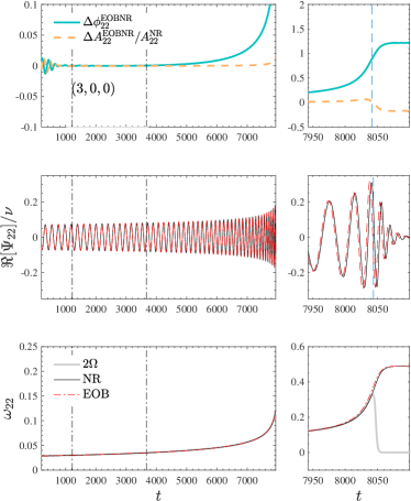
Figure 2: Example of acceptable EOB/NR phasing agreement obtained suitably selecting the value of $a_{6}^{c}$ for $(q,\chi_{1},\chi_{2})=(3,0,0)$. The NR dataset used here is SXS:BBH:1221.

We now proceed in determining new analytical representations of $(a_{6}^{c},c_{3})$. The procedure is the same as the one discussed in Ref. Nagar et al. (2021b): one first determines the best $a_{6}^{c}$ and then the best $c_{3}$ by analyzing EOB/NR phasing comparisons. Figure 2 displays an example of what we consider an acceptable choice of the parameter, $a_{6}^{c}=-78$, informed by the inspection of the EOB/NR phase difference $\Delta\phi_{22}^{\rm EOBNR}$. When the two waveforms are aligned during the early inspiral (the alignment region is indicated by the dashed-dot vertical lines), the phase difference starts practically flat and then grows monotonically through plunge and merger until it ends up constant during ringdown. We have $\Delta\phi_{22}^{\rm EOBNR}\sim 1$ rad at merger, that is larger than the numerical uncertainty ($\sim 0.1$ rad), but it is small enough to yield values ($<1\%$) of the EOB/NR unfaithfulness (see below). In addition, the phase difference accumulated up to merger is still larger than the one for the quasi-circular TEOBResumS model, as shown in Fig. 3. However, we explored the flexibility of the model varying $a_{6}^{c}$ and we eventually concluded that within the current analytical setup it is not possible to further flatten $\Delta\phi_{22}^{\rm EOBNR}$ and get it close to the quasi-circular case. The dotted gray line in Fig. 3 refers to $a_{6}^{c}=-71$ and gives an idea of the flexibility of the model when $a_{6}^{c}$ is varied. Increasing $a_{6}^{c}$ goes in the direction of reducing the accumulated phase difference; however, this parameter alone is unable to flatten the phase difference at the same level of the quasi-circular case (see in particular left panel of Fig. 3). Moreover, the fact that the phasing is at $~{}\sim 0.1$ level during the ringdown but it is larger up to merger may eventually result in suboptimal values of the EOB/NR unfaithfulness. This can also be understood by looking at the EOB/NR phase difference when the waves are aligned around merger and not during the inspiral. Although we could not overcome this problem, we realized that this is related to structure of ${\cal F}_{r}$, that is given by Eq. (6) of Ref. Nagar et al. (2021b), and in particular to the leading order factor given by $p_{r_{*}}u^{4}$, as obtained Ref. Bini and Damour (2012). Some alternative analytical expression at leading order might be worth exploring, although we postpone this investigation to future work. In conclusion, when tuning $a_{6}^{c}$ with NR data we were careful to obtain phase differences that are always monotonic versus time, in order to reproduce the qualitative structure of the $a_{6}^{c}=-78$ phase difference in Fig. 3.

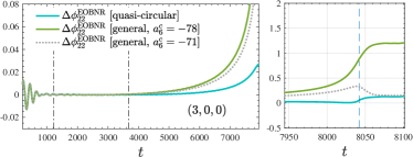
Figure 3: Comparing phasings for different EOB models or values of $a_{6}^{c}$ for $(q,\chi_{1},\chi_{2})=(3,0,0)$, SXS:BBH:1221. The EOB/NR phase agreement of the general model (for various values of $a_{6}^{c}$, see text) up to merger is acceptable, but is significantly worse than for the simple quasi-circular model.

Table 1: Informing the nonspinning sector of the model. From left to right the columns report: the dataset number, the SXS identification number; the mass ratio $q$; the symmetric mass ratio $\nu$; the first guess value of $a_{6}^{c}$ and the fitted value from Eq. (41).

$\#$	SXS	$q$	$\nu$	$a_{6}^{c}$	$a_{6}^{c}(\nu)$
1	SXS:BBH:0180	1	0.25	$-93$	$-93.0372$
2	SXS:BBH:1221	3	0.204	$-78$	$-77.969$
3	SXS:BBH:0056	6	0.139	$-58$	$-57.308$
4	SXS:BBH:0063	8	0.0988	$-47$	$-48.525$
5	SXS:BBH:0303	10	0.0826	$-43$	$-42.161$

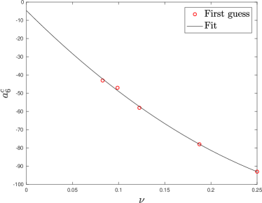
Figure 4: First-guess values of $a_{6}^{c}$ from Table 1. Note the rather simple functional behavior of $a_{6}^{c}(\nu)$ with respect to Ref. Nagar et al. (2021b), see in particular Eq. (14) therein. This fact suggests that the new analytical building blocks have simplified the impact of NR information in the completion of the model.

Table 2: Informing the spinning sector of the model. From left to right the columns report: the dataset number, the SXS identification number; the mass ratio and the individual dimensionless spins $(q,\chi_{1},\chi_{2})$; the first-guess values of $c_{3}$ used to inform the global interpolating fit given in Eq. (III.1), and the corresponding $c_{3}^{\rm fit}$ values.

$\#$	ID	$(q,\chi_{1},\chi_{2})$	$c_{3}^{\rm first\;guess}$	$c_{3}^{\rm fit}$
1	SXS:BBH:0156	$(1,-0.95,-0.95)$	89	88.822
2	SXS:BBH:0159	$(1,-0.90,-0.90)$	86.5	86.538
3	SXS:BBH:0154	$(1,-0.80,-0.80)$	81	81.508
4	SXS:BBH:0215	$(1,-0.60,-0.60)$	70.5	70.144
5	SXS:BBH:0150	$(1,+0.20,+0.20)$	26.5	26.677
6	SXS:BBH:0228	$(1,+0.60,+0.60)$	16.0	15.765
7	SXS:BBH:0230	$(1,+0.80,+0.80)$	13.0	12.920
8	SXS:BBH:0153	$(1,+0.85,+0.85)$	12.0	12.278
9	SXS:BBH:0160	$(1,+0.90,+0.90)$	11.5	11.595
10	SXS:BBH:0157	$(1,+0.95,+0.95)$	11.0	10.827
11	SXS:BBH:0004	$(1,-0.50,0)$	54.5	46.723
12	SXS:BBH:0231	$(1,+0.90,0)$	24.0	23.008
13	SXS:BBH:0232	$(1,+0.90,+0.50)$	15.8	16.082
14	SXS:BBH:0005	$(1,+0.50,0)$	34.3	27.136
15	SXS:BBH:0016	$(1.5,-0.50,0)$	57.0	49.654
16	SXS:BBH:0016	$(1.5,+0.95,+0.95)$	13.0	11.720
17	SXS:BBH:0255	$(2,+0.60,0)$	29.0	23.147
18	SXS:BBH:0256	$(2,+0.60,+0.60)$	20.8	17.37
19	SXS:BBH:0257	$(2,+0.85,+0.85)$	14.7	14.56
20	SXS:BBH:0036	$(3,-0.50,0)$	60.0	53.095
21	SXS:BBH:0267	$(3,-0.50,-0.50)$	69.5	60.37
22	SXS:BBH:0174	$(3,+0.50,0)$	30.0	24.210
23	SXS:BBH:0291	$(3,+0.60,+0.60)$	23.4	19.635
24	SXS:BBH:0293	$(3,+0.85,+0.85)$	16.2	17.759
25	SXS:BBH:1434	$(4.368,+0.80,+0.80)$	20.3	20.715
26	SXS:BBH:0060	$(5,-0.50,0)$	62.0	55.385
27	SXS:BBH:0110	$(5,+0.50,0)$	31.0	24.488
28	SXS:BBH:1375	$(8,-0.90,0)$	64.0	71.91
29	SXS:BBH:0064	$(8,-0.50,0)$	57.0	55.385
30	SXS:BBH:0065	$(8,+0.50,0)$	28.5	24.306

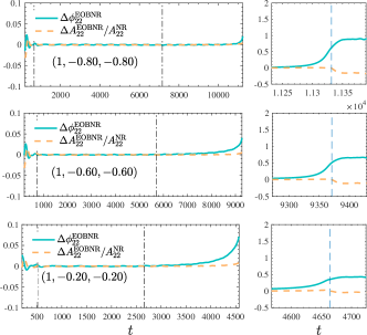
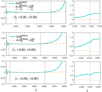
Figure 5: EOB/NR time-domain phase difference $\Delta\phi_{22}^{\rm EOBNR}$ and relative amplitude difference, $\Delta A^{\rm EOBNR}_{22}/A^{\rm NR}_{22}$ for a sample of equal-mass, equal-spin configurations. The model uses here the $c_{3}$ parameter from Eq. (III.1). The dash-dotted vertical lines indicate the alignment region, while the dashed line indicates the merger location. Note that $\bar{F}_{\rm EOBNR}^{\rm max}\lesssim 1\%$ even if the accumulated phase difference $\sim 1$ rad at merger for some configurations.

We determined $a_{6}^{c}$ separately for different 5 datasets, listed in Table 1: the fifth column of the table reports our best choices. When plotted versus $\nu$, one finds a rather simple behavior, see Fig. 4, that is fitted as

$$a_{6}^{c}(\nu)=599.96\nu^{2}-503.57\nu-4.6416.$$ (41)

The fit is very accurate, as shown by the sixth column of Table 1. In this respect, it is interesting to note that, although the physics that the model describes is the same of the model of Ref. Nagar et al. (2021b), the differences in the analytical content and in the resummations yield a very simple behavior of $a_{6}^{c}(\nu)$. This is in striking contrast with Ref. Nagar et al. (2021b), where it was needed an exponential function to fit (at a lower accuracy level) the single values of $a_{6}^{c}$.

The new functional form of $a_{6}^{c}(\nu)$ given by Eq. (41) calls for a similarly new determination of the effective spin-orbit parameter $c_{3}$. We do so using a set of NR data that is slightly different from the one used in Ref. Nagar et al. (2020) so to improve the robustness of the model in certain corners of the parameter space. The NR datasets used are listed in Table 2. Following Ref. Nagar et al. (2020), for each dataset we report the value of $c_{3}^{\rm first\;guess}$ obtained by comparing EOB and NR phasing so that the accumulated phase difference is of the order of the NR uncertainty (and/or so that consistency between NR and EOB frequencies around merger is achieved as much as possible). Similarly to the case of $a_{6}^{c}$, the robustness of the model allows us to efficiently do this by hand without any automatized procedure. The $c_{3}^{\rm first\;guess}$ values of Table 2 are fitted with a global function of the spin variables $\tilde{a}_{i}\equiv S_{i}/(m_{i}M)$ with $i=1,2$ of the form

$$c_{3}(\tilde{a}_{1},\tilde{a}_{2},\nu)=p_{0}\dfrac{1+n_{1}\tilde{a}_{0}+n_{2}\tilde{a}_{0}^{2}+n_{3}\tilde{a}_{0}^{3}+n_{4}\tilde{a}_{0}^{4}}{1+d_{1}\tilde{a}_{0}}$$

$$+p_{1}\tilde{a}_{0}\nu\sqrt{1-4\nu}+p_{2}\left(\tilde{a}_{1}-\tilde{a}_{2}\right)\nu^{2}+p_{3}\tilde{a}_{0}\nu^{2}\sqrt{1-4\nu},$$ (42)

where $\tilde{a}_{0}\equiv\tilde{a}_{1}+\tilde{a}_{2}$ and the functional form is the same of previous works. This term helps in improving the fit flexibility as the mass ratio increases. The fitting coefficients read

$$p_{0} =35.482253,$$ (43)

$$n_{1} =-1.730483,$$ (44)

$$n_{2} =1.144438,$$ (45)

$$n_{3} =0.098420,$$ (46)

$$n_{4} =-0.329288,$$ (47)

$$d_{1} =-0.345207,$$ (48)

$$p_{1} =244.505,$$ (49)

$$p_{2} =148.184,$$ (50)

$$p_{3} =-1085.35.$$ (51)

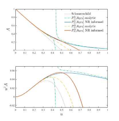
Figure 6: Comparison between different $A$ functions (top panel) and effective photon potentials, $u^{2}A$ (bottom panel) for $q=1$. The picture highlights that the commonly used $P^{1}_{5}[A]$ approximant develops an unphysical pole when $a_{6}^{c}=a_{6\rm anlyt}^{c}$ from Eq. (II.1). One also notices the consistency between the two NR-informed $A$ functions up to the effective light-ring, i.e. the peak of the function $u^{2}A$. Note however that the difference between the potentials around $u\simeq 0.4$ is $\sim 10^{-2}$, so that they do actually yield different EOB dynamics.

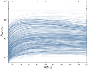
Figure 7: Unfaithfulness $\bar{F}_{\rm EOB/NR}(M)$ between the quasi-circular limit of the general TEOBResumS model and the complete SXS catalog of non-eccentric and non-precessing (spin-aligned) waveforms. These results are obtained using the NR-tuned N³LO spin-orbit contribution. The horizontal dotted lines mark the $0.01$ (black) and $0.03$ (blue) values.

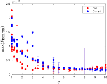
Figure 8: Complement to Fig. 7: $\bar{F}^{\rm max}_{\rm EOB/NR}$ values for all SXS nonspinning configurations. The current iteration of TEOBResumS is compared to the quasi-circular model of Ref. Nagar et al. (2020), with errorbars that represent the values of $\bar{F}^{\rm max}_{\rm NR/NR}$ cited therein (see Tables XVIII-XIX). Note that SXS datasets with the same $q$ have different NR accuracies. The EOB/NR agreement for this subset of data is largely improved with respect to Fig. 3 of Ref. Nagar et al. (2021b) and mostly consistent with the result of the quasi-circular model.

III.1.1 Consistency between EOB potentials

Now that we have determined the new expression of $a_{6}^{c}(\nu)$ it is instructive to compare different realization of the potential. The top panel of Fig. 6 shows together different curves for the case $q=1$: (i) The $P^{3}_{3}[A]$ potential with the NR-informed $a_{6}^{c}(\nu)$ given by Eq. (41) above; (ii) the $P^{1}_{5}[A]$ potential of TEOBResumS, where the NR-informed function is given by Eq. (33) of Ref. Nagar et al. (2020); (iii) the $P^{1}_{5}[A]$ function with $a_{6}^{c}=a^{c}_{6\rm anlyt}$; (iv) the $P^{3}_{3}[A]$ function with $a_{6}^{c}=a^{c}_{6\rm anlyt}$. In the bottom panel of the figure we show the effective photon potential $u^{2}A$. The most interesting outcome is the visual consistency between the two NR-informed potentials up to $u\simeq 0.4$. This reflects in two close dynamics, that eventually yield highly faithful EOB/NR phasing for the nonspinning case, as we will see below. The fact is remarkable because both the radiation reaction and the $(D,Q)$ potentials are different in the two cases. One should note, however, that the fact that the two potentials are consistent up to $u=0.4$ does not mean that they are equivalent and that the conservative dynamics coincide. In fact, it is known Damour et al. (2013) that two $A$ potentials are equivalent when their difference is of the order of $10^{-4}$. The two NR-informed potentials differ by just $10^{-2}$, so that even if they look close, they are meaningfully different. A similar visual consistency shows up also for the $P^{1}_{5}[A]$ analytical function, despite the presence of the spurious pole. By contrast the fully analytical $P^{3}_{3}[A]$ is significantly separated from the others. In practical terms, when used in the EOB dynamics, the $P^{3}_{3}[A]$ analytical potential will accelerate the inspiral with respect to the NR-informed ones, eventually yielding unacceptably large phase differences at merger. If one wished to incorporate this specific resummation, some other element of the model (e.g. radiation reaction or the $(D,Q)$ functions) should be modified to balance its attractive effect. This gives a pedagogical example of the fact that the accessibility of high-order PN information does not necessarily simplify or help the construction of waveform models and it is pragmatically more efficient to resort to NR-informed functions.

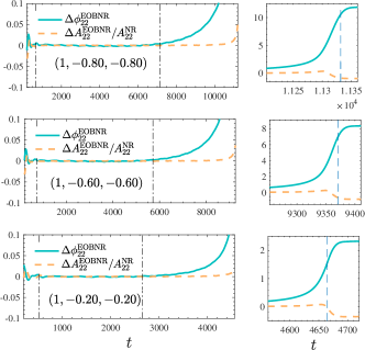
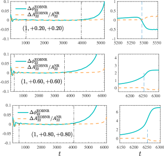
Figure 9: EOB/NR time-domain phase difference $\Delta\phi_{22}^{\rm EOBNR}$ and relative amplitude difference, $\Delta A^{\rm EOBNR}_{22}/A^{\rm NR}_{22}$ for a sample of equal-mass, equal-spin configurations. The model uses here the analytical description of N³LO spin-orbit effect, with $c_{4}=0$. The dash-dotted vertical lines indicate the alignment region, while the dashed line indicates the merger location. The large values of $\Delta\phi_{22}^{\rm EOBNR}$ at merger eventually end up with values of $\bar{F}_{\rm EOBNR}^{\rm max}$ even above the $3\%$ level, see Fig. 10 below.

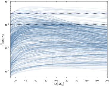
Figure 10: Unfaithfulness $\bar{F}_{\rm EOB/NR}(M)$ between TEOBResumS and the complete SXS catalog of non-eccentric non-precessing waveforms obtained using the analytical N³LO spin-orbit contribution. The horizontal dotted lines mark the $0.01$ (black) and $0.03$ (blue) values.

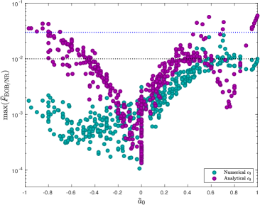
Figure 11: Global picture of the maximum EOB/NR unfaithfulness from Fig. 7 and Fig. 10 using the NR-informed and the analytical N³LO spin-orbit contribution respectively. The black and blue dotted lines mark the $0.01$ and $0.03$ values respectively. The use of the analytical spin-orbit contribution delivers a NR-faithful model only in a rather limited range of $\tilde{a}_{0}$.

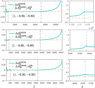
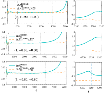
Figure 12: EOB/NR time-domain phase difference $\Delta\phi_{22}^{\rm EOBNR}$ and relative amplitude difference, $\Delta A^{\rm EOBNR}_{22}/A^{\rm NR}_{22}$ for a sample of equal-mass, equal-spin configurations. The model uses here the analytical description of N³LO spin-orbit effect augmented by a NR-tuned coefficient $c_{4}$ at N⁴LO, as given by Eq. (53). The dash-dotted vertical lines indicate the alignment region, while the dashed line indicates the merger location. The phase difference at merger is reduced with respect to the $c_{4}=0$ case of Fig. 9, although it is still slightly less good (especially for negative spins) than the simple NR-tuned $c_{3}$ case of Fig. 5.

III.1.2 Validating the model

To evaluate the quality of the EOB waveform we computed the EOB/NR unfaithfulness weighted by the Advanced LIGO noise over all available spin-aligned SXS configurations. Considering two waveforms $(h_{1},h_{2})$, the unfaithfulness is a function of the total mass $M$ of the binary and is defined as

$$\bar{F}(M)\equiv 1-F=1-\max_{t_{0},\phi_{0}}\dfrac{\langle h_{1},h_{2}\rangle}{||h_{1}||||h_{2}||},$$ (52)

where $(t_{0},\phi_{0})$ are the initial time and phase. We used $||h||\equiv\sqrt{\langle h,h\rangle}$, and the inner product between two waveforms is defined as $\langle h_{1},h_{2}\rangle\equiv 4\Re\int_{f_{\rm min}^{\rm NR}(M)}^{\infty}\tilde{h}_{1}(f)\tilde{h}_{2}^{*}(f)/S_{n}(f)\,df$, where $\tilde{h}(f)$ denotes the Fourier transform of $h(t)$, $S_{n}(f)$ is the zero-detuned, high-power noise spectral density of Advanced LIGO aLI and $f_{\rm min}^{\rm NR}(M)=\hat{f}^{\rm NR}_{\rm min}/M$ is the initial frequency of the NR waveform at highest resolution, i.e. the frequency measured after the junk-radiation initial transient. Waveforms are tapered in the time-domain so as to reduce high-frequency oscillations in the corresponding Fourier transforms. The EOB/NR unfaithfulness is addressed as $\bar{F}_{\rm EOB/NR}$. The result of this computation is shown in Fig. 7. We can see that the maximum unfaithfulness is mostly below $0.01$ and always below $0.03$. We will highlight in Fig. 11 below that the higher $\bar{F}_{\rm EOB/NR}$ correspond to configuration with large spin values, aligned with the orbital angular momentum.

Before doing so, it is instructive also to show separately the $\bar{F}_{\rm EOB/NR}^{\rm max}$ restricted to the nonspinning case. The chosen NR waveforms are listed in Tables XVIII-XIX of Ref. Nagar et al. (2020), with the exclusion of the 3 BAM Husa et al. (2016) ones and 6 precessing configurations that were erroneously included there . To better appreciate the improvement with respect to Ref. Nagar et al. (2021b), Fig. 8 compares the current (nonspinning) $\bar{F}_{\rm EOB/NR}^{\rm max}$ values with those of TEOBResumS obtained in Ref. Nagar et al. (2020). There is an excellent consistency between the two dataset, although the current model is performing slightly less well up to $q=4$. This is expected in view of the discussion around Fig. 3.

III.2 Fully analytical effective one body spin-orbit dynamics at N³LO and beyond

Table 3: Informing the N⁴LO spin-orbit effective contribution. From left to right the columns report: the dataset number, the SXS identification number; the mass ratio and the individual dimensionless spins $(q,\chi_{1},\chi_{2})$; the first-guess values of $c_{4}$ used to inform the global interpolating fit given in Eq. (III.1), and the corresponding $c_{4}^{\rm fit}$ values.

$\#$	ID	$(q,\chi_{1},\chi_{2})$	$\tilde{a}_{0}$	$c_{4}^{\rm first\;guess}$	$c_{4}^{\rm fit}$
1	SXS:BBH:0156	$(1,-0.95,-0.95)$	$-0.95$	230	235.99
2	SXS:BBH:0154	$(1,-0.80,-0.80)$	$-0.80$	210	204.38
3	SXS:BBH:0215	$(1,-0.60,-0.60)$	$-0.60$	163	164.98
4	SXS:BBH:	$(1,-0.20,-0.20)$	$-0.20$	107.5	95.66
4	SXS:BBH:0150	$(1,+0.20,+0.20)$	$+0.20$	28	38.95
5	SXS:BBH:0228	$(1,+0.60,+0.60)$	$+0.60$	$-8$	$-5.14$
6	SXS:BBH:0230	$(1,+0.80,+0.80)$	$+0.80$	$-21$	$-22.45$
10	SXS:BBH:0157	$(1,+0.95,+0.95)$	$+0.95$	$-30.5$	$-33.36$

Table 4: SXS simulations with eccentricity analyzed in this work. From left to right: the ID of the simulation; the mass ratio $q\equiv m_{1}/m_{2}\geq 1$ and the individual dimensionless spins $(\chi_{1},\chi_{2})$; the time-domain NR phasing uncertainty at merger $\delta\phi^{\rm NR}_{\rm mrg}$; the estimated NR eccentricity at first apastron $e_{\omega_{a}}^{\rm NR}$; the NR frequency of first apastron $\omega_{a}^{\rm NR}$; the initial EOB eccentricity $e^{\rm EOB}_{\omega_{a}}$ and apastron frequency $\omega_{a}^{\rm EOB}$ used to start the EOB evolution; the maximal NR unfaithfulness uncertainty, $\bar{F}^{\rm max}_{\rm NR/NR}$ and the maximal EOB/NR unfaithfulness, $\bar{F}_{\rm EOB/NR}^{\rm max}$.

$\#$	id	$(q,\chi_{1},\chi_{2})$	$\delta\phi^{\rm NR}_{\rm mrg}$[rad]	$e^{\rm NR}_{\omega_{a}}$	$\omega_{a}^{\rm NR}$	$e^{\rm EOB}_{\omega_{a}}$	$\omega_{a}^{\rm EOB}$	$\bar{F}_{\rm NR/NR}^{\rm max}[\%]$	$\bar{F}_{\rm EOB/NR}^{\rm max}[\%]$
1	SXS:BBH:1355	$(1,0,0)$	$+0.92$	0.0620	0.03278728	0.0888	0.02805750	0.012	0.13
2	SXS:BBH:1356	$(1,0,0)$	$+0.95$	0.1000	0.02482006	0.15038	0.019077	0.0077	0.17
3	SXS:BBH:1358	$(1,0,0)$	$+0.25$	0.1023	0.03108936	0.18078	0.021238	0.016	0.17
4	SXS:BBH:1359	$(1,0,0)$	$+0.25$	0.1125	0.03708305	0.18240	0.02139	0.0024	0.13
5	SXS:BBH:1357	$(1,0,0)$	$-0.44$	0.1096	0.03990101	0.19201	0.01960	0.028	0.11
6	SXS:BBH:1361	$(1,0,0)$	+0.39	0.1634	0.03269520	0.23557	0.0210	0.057	0.38
7	SXS:BBH:1360	$(1,0,0)$	$-0.22$	0.1604	0.03138220	0.2440	0.01953	0.0094	0.31
8	SXS:BBH:1362	$(1,0,0)$	$-0.09$	0.1999	0.05624375	0.3019	0.01914	0.0098	0.13
9	SXS:BBH:1363	$(1,0,0)$	$+0.58$	0.2048	0.05778104	0.30479	0.01908	0.07	0.25
10	SXS:BBH:1364	$(2,0,0)$	$-0.91$	0.0518	0.03265995	0.08464	0.025231	0.049	0.12
11	SXS:BBH:1365	$(2,0,0)$	$-0.90$	0.0650	0.03305974	0.11015	0.023987	0.027	0.096
12	SXS:BBH:1366	$(2,0,0)$	$-6\times 10^{-4}$	0.1109	0.03089493	0.1496	0.02580	0.017	0.30
13	SXS:BBH:1367	$(2,0,0)$	$+0.60$	0.1102	0.02975257	0.15065	0.026025	0.0076	0.18
14	SXS:BBH:1368	$(2,0,0)$	$-0.71$	0.1043	0.02930360	0.14951	0.02527	0.026	0.34
15	SXS:BBH:1369	$(2,0,0)$	$-0.06$	0.2053	0.04263738	0.3134	0.01735	0.011	0.21
16	SXS:BBH:1370	$(2,0,0)$	$+0.12$	0.1854	0.02422231	0.3149	0.01688	0.07	0.46
17	SXS:BBH:1371	$(3,0,0)$	$+0.92$	0.0628	0.03263026	0.0912	0.029058	0.12	0.17
18	SXS:BBH:1372	$(3,0,0)$	$+0.01$	0.1035	0.03273944	0.14915	0.026070	0.06	0.07
19	SXS:BBH:1373	$(3,0,0)$	$-0.41$	0.1028	0.03666911	0.15035	0.0253	0.0034	0.17
20	SXS:BBH:1374	$(3,0,0)$	$+0.98$	0.1956	0.02702594	0.314	0.016938	0.067	0.08
21	SXS:BBH:89	$(1,-0.50,0)$	$\dots$	0.0469	0.02516870	0.07199	0.01779	$\dots$	0.14
22	SXS:BBH:1136	$(1,-0.75,-0.75)$	$-1.90$	0.0777	0.04288969	0.12105	0.02728	0.074	0.10
23	SXS:BBH:321	$(1.22,+0.33,-0.44)$	$+1.47$	0.0527	0.03239001	0.07621	0.02694	0.015	0.21
24	SXS:BBH:322	$(1.22,+0.33,-0.44)$	$-2.02$	0.0658	0.03396319	0.0984	0.026895	0.016	0.20
25	SXS:BBH:323	$(1.22,+0.33,-0.44)$	$-1.41$	0.1033	0.03498377	0.1438	0.02584	0.019	0.15
26	SXS:BBH:324	$(1.22,+0.33,-0.44)$	$-0.04$	0.2018	0.02464165	0.29421	0.01894	0.098	0.24
27	SXS:BBH:1149	$(3,+0.70,+0.60)$	$+3.00$	0.0371	0.03535964	$0.0621$	$0.02664$	0.025	0.96
28	SXS:BBH:1169	$(3,-0.70,-0.60)$	$+3.01$	0.0364	0.02759632	$0.04895$	$0.024285$	0.033	0.10

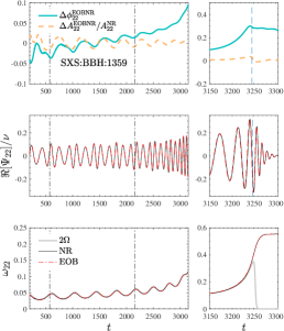
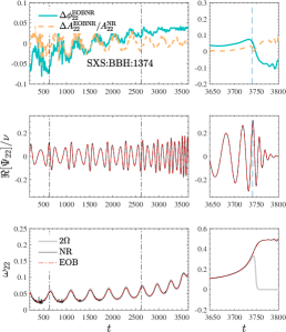
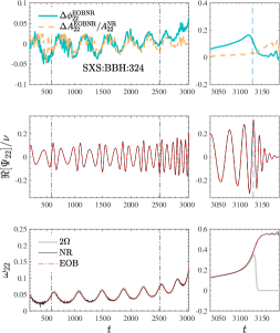
Figure 13: EOB/NR time-domain phasing comparison three meaningful configurations SXS:BBH:1359, SXS:BBH:1374 and SXS:BBH:324. The phasing agreement is largely improved with respect to the corresponding ones shown in Fig. 10 of Ref. Nagar et al. (2021b). The vertical dash-dotted lines in the left panels indicate the alignment interval, while the merger location is marked by a dashed vertical line in the right panels.

Let us finally evaluate the EOB/NR performance using the fully analytical expression for the N³LO spin-orbit contribution. First of all, Fig. 9 displays time-domain phasing comparisons for the same $q=1$ configurations considered above. The phase differences at merger are rather larger, especially for large values of the individual spins. The EOB/NR unfaithfulness computation is reported in Fig. 10: one finds that there are many configuration even above the fiducial threshold of $3\%$. To have a simple understanding of the inaccurate configurations it is helpful to plot $\bar{F}_{\rm EOB/NR}^{\rm max}$ versus the effective spin $\tilde{a}_{0}$, Fig. 11. One sees that the EOB/NR agreement degrades progressively as the effective spin increases or decreases. In practice, the analytical model can be considered robustly faithful ($<1\%$) only for mild values of the effective spin. Note however that there is a region where $\bar{F}^{\rm max}_{\rm EOB/NR}<1\%$ also for large, positive spins. This corresponds roughly to simulations where $0.6\lesssim\tilde{a}_{0}\lesssim 0.8$ and $q<5$. For completeness, the same plot also reports (with green markers) the values of $\bar{F}^{\rm max}_{\rm EOB/NR}$ for the NR-informed value of $c_{3}$, so to give complementary information to the one of Fig. 7. To conclude, what is striking in this comparison is that, similarly to the case of $a_{6}^{c}$ mentioned above a suitably NR-tuned effective function is pragmatically more efficient than the outcome of a high-order analytical calculation.

In this respect, we recall that in our definitions of $(G_{S},G_{S_{*}})$ we introduced two formal N⁴LO terms, where $c_{40}^{*}=2835/256$, fixed to the spinning test-mass value. However, analogously to the case of $c_{3}$, we can flex these two coefficients as $c_{40}=\nu c_{4}u_{c}^{4}$ and $c_{40}^{*}=\nu c_{4}+2835/256$ introducing an effective N⁴LO parameter that can be tuned to NR simulations analogously to $c_{3}$. We show this here explicitly by determining $c_{4}$ for the specific case of equal-mass, equal spin binaries and evaluating the resulting performance in terms of phasing.

Let us start by inspecting Fig. 9. The EOB/NR phase difference is always positive. However, the physical meaning of this observation is different whether the spins are aligned or anti-aligned with the orbital angular momentum. Let us start with the case $(1,+0.60,+0.60)$, middle right panel of Fig. 9. The fact that the sign is positive indicates that the transition from inspiral to plunge and merger occurs faster than the NR prediction, so to yield an accumulated phase difference of 1.5 rad at merger. Within the EOB Hamiltonian, this effect is interpreted as an underestimation of the spin-orbit interaction with respect to the NR case. To contrast this fact, one should reduce the phase acceleration, or, in other words, increase the spin-orbit interaction so that its repulsive character (because spins are aligned with the orbital angular momentum) becomes larger. Similarly, for the case $(1,-0.60,-0.60)$ with $c_{4}=0$ one again finds that the EOB plunge phase is more accelerated than the corresponding NR one, but now the motivation is different: the spin-orbit interaction is now too large and it should be reduced. To probe that $c_{4}$ can be tuned the same way as $c_{3}$, we consider a small set of equal-mass, equal-spin configurations, see Table 3. The table lists the first-guess values of $c_{4}$ that are found to yield an acceptable ($\lesssim 1$ rad) phase difference at merger time. The interesting fact is that, analogously to the $c_{3}$ case, the magnitude of the effective parameter increases as the spins become large and negative. These $c_{4}$ data can be fitted by a quadratic function of $\tilde{a}_{0}$, yielding the following function

$$c_{4}=39.43\tilde{a}_{0}^{2}-141.77\tilde{a}_{0}+65.73.$$ (53)

The corresponding time-domain comparison (either phase difference and amplitude difference) are shown in Fig. 12. The phase difference at merger is notably reduced with respect to the $c_{4}=0$ case of Fig. 9, although it is still slightly less good than the simple NR-tuned $c_{3}$ case of Fig. 5. It seems thus that the use of the complete analytical N³LO spin-orbit information within the current model just moves the need of a NR-tuned parameter at the N⁴LO order with slightly less accuracy and with no real advantage. This suggests that, within the current model, it is more efficient to simply adopt the NR-tuned $c_{3}$ parameter.

IV Eccentric inspiral configurations

Let us move now to discussing eccentric inspirals. To do so, we precisely repeat here the analysis of Ref. Nagar et al. (2021b), see Secs. IIIC and IIID therein. The initial conditions are slightly fine tuned with respect to Ref. Nagar et al. (2021b), so that Table 4 is an updated version of Table III of Ref. Nagar et al. (2021b). All NR quantities are evidently the same. The EOB quantities are coming with updated computations with the model discussed here, in particular one notices: (i) new initial conditions $(e_{\omega_{a}}^{\rm EOB},\omega_{a}^{\rm EOB})$ and (ii) new values of the maximum of the EOB/NR unfaithfulness $\bar{F}^{\rm max}_{\rm EOB/NR}$. To start with, Fig. 13 reports the $\ell=m=2$ time-domain phasing comparison for SXS:BBH:1359, SXS:BBH:1374 and SXS:BBH:324. For each configuration, (i) at the top we have the phase difference and the relative amplitude difference; (ii) in the middle we compare the real parts of the waveform; (iii) in the bottom panel we compare the EOB and NR GW frequency, together with twice the orbital frequency $\Omega$. The phasing agreement is largely improved with respect to what shown in Fig. 10 and Fig. 14 of Ref. Nagar et al. (2021b): the EOB/NR phase difference is rather low and does not vary much during the inspiral and remains of the order of $0.1-0.2$ rad up to merger as well.

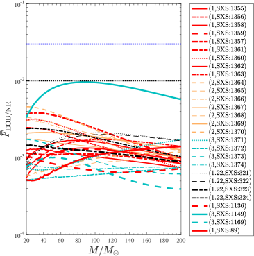
Figure 14: EOB/NR unfaithfulness for the $\ell=m=2$ mode computed over the eccentric SXS simulations publicly available, Table 4. The horizontal lines mark the 0.03 and 0.01 values. All configurations are well below the $1\%$ except for SXS:BBH:1149, corresponding to $(3,+0.70,+0.60)$ with $e_{\omega_{a}}^{\rm NR}=0.037$, that is grazing this value. This is consistent with the slight degradation of the model performance for large positive spins, as found in the quasi-circular limit.

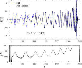
Figure 15: Illustrative example of the tapering procedure for SXS:BBH:1362. Note that the junk radiation in the NR dataset is practically absent.

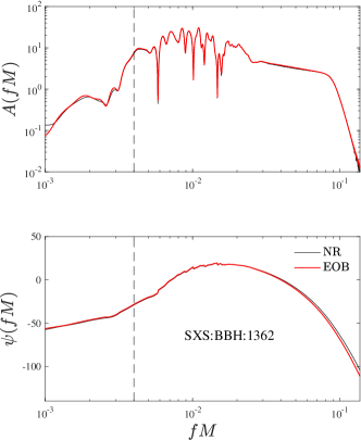
Figure 16: Comparing the NR (black) and EOB (red online) Fourier transforms for the SXS:BBH:1362 configuration: amplitude ( $A(fM)$, top panel) and phase ($\psi(fM)$, bottom panel). The vertical dashed line indicates the lowest boundary of integration to be used to compute the unfaithfulness from Eq. (52). Note that to accurately capture the oscillatory behavior of $A(fM)$ the time-domain vectors are padded with zeros before doing the Fourier transform. The part before the maximum of the amplitude (say $fM\lesssim 6\times 10^{-3}$, approximately corresponding to a kink in $\psi(Mf)$) has little influence on $\bar{F}_{\rm EOB/NR}$ so that the initial frequency can be augmented up to this value without relevant consequences. See text for additional discussion.

The global vision of the model performance is given by Fig. 14, that highlights the EOB/NR unfaithfulness versus the total mass of the system. We find that all configurations are well below $1\%$ except for SXS:BBH:1149, that is grazing this value. This is not surprising since SXS:BBH:1149 has parameter $(3,+0.7,+0.6)$, that give $\tilde{a}_{0}=0.675$, a value that belongs to the region of $\tilde{a}_{0}$ where it is not possible to obtain a highly NR-faithful modelization already in the quasi-circular case. Despite this, the improvements in the quasi-circular sector reflect all over the $\bar{F}_{\rm EOB/NR}$ behavior of Fig. 14, either for small or for large eccentricities. This is in particular the case for the $q=1$ configurations, where $\bar{F}_{\rm EOB/NR}$ gets down to $\sim 10^{-3}$. This is a remarkable improvement with respect to the results of Ref. Nagar et al. (2021b), where $\bar{F}_{\rm EOB/NR}$ was grazing the $1\%$ threshold for these configurations (see Fig. 11 therein). In this respect, in redoing the $\bar{F}_{\rm EOB/NR}$ calculation for the current model, we realized that Ref. Nagar et al. (2021b), overlooked the importance of the resolution employed in the calculation of the Fourier transforms and its eventual impact on the results. We thus revised and updated also the $\bar{F}_{\rm EOB/NR}$ calculation of Ref. Nagar et al. (2021b), that is now discussed in Appendix A. Entering the details, let us first recall that the NR signal is tapered before doing the Fourier transform so as to reduce high-frequency spurious oscillations. Figure 15 illustrates this procedure (obtained multiplying the waveform by an hyperbolic tangent function) on the NR dataset SXS:BBH:1362. When one then takes the Fourier transform, we found it necessary (as already mentioned in Ref. Hinder et al. (2017)) to pad the time-domain vectors with zeros in order to increase the frequency resolution and capture all the details at low frequency. The Fourier transform of the NR signal is shown in Fig. 16 together with the one of the corresponding EOB waveform (red online). The top-panel reports the amplitude $A(fM)$ and the bottom panel the phase $\psi(fM)$ [we assumed that $\tilde{h}=A(fM)e^{i\psi(fM)}$]. To accurately capture all the oscillatory behavior of the modulus, and also to avoid unphysical features in the phase, we use here frequency resolutions $M\delta f\sim 10^{-4}$. For each NR dataset we have been careful to progressively increase the resolution until the calculation of $\psi(fM)$ becomes robust. The same is done also for the EOB waveform, with the distinction that the corresponding tapering should be chosen so to match as much as possible the behavior of the corresponding NR waveform. Figure 16 refers to the SXS:BBH:1362 dataset, although the behavior is however typical for all other configurations. The vertical line, located at $fM=0.004$, indicates the lower integration boundary, $Mf_{\rm min}$ in the unfaithfulness computation for this configuration. From Fig. 15 this value is close to the minimal frequency reached at the first apastron. Clearly, the value of $Mf_{\rm min}$ may vary from one dataset to the other, although it is chosen to be always lower than the maximum of $A(fM)$. In any case, the part of the signal up to the amplitude maximum (say up to $fM\sim 0.006$ in this case) has negligible influence on the total result. In obtaining the $\bar{F}_{\rm EOB/NR}$ results displayed in Fig. 14 we have been careful to obtain EOB/NR visual agreement between the Fourier transforms of each dataset analogous to the one shown in Fig. 16 for the SXS:BBH:1362 dataset.

Given the exploratory character of the current study, we have just briefly looked at higher modes. The NR-accurate behavior of all waveform modes during the inspiral is comparable to what discussed in Ref. Nagar et al. (2021b). By contrast, for what concerns merger and ringdown, although the modes with $m=\ell$ usually (though not always) look generally sane, those with $m\neq\ell$ may develop unphysical behaviors due to the action of NQC corrections, as already noted in Ref. Nagar et al. (2021b). This problem, that has always been present within TEOBResumS Nagar et al. (2018), is now even amplified because of the existence of an effective horizon corresponding to the fact that the $A$ function has a zero at a finite value of $u$. The issue of robustly determining NQC corrections for any multipole will require more dedicated investigations, that we will postpone to future work. We only anticipate that it is likely that a deeper understanding of NQC corrections (especially in relation with the dynamics) in the test-mass limit Albanesi et al. (2021) will be required to overcome what currently seems to be the most evident Achilles’ heel of TEOBResumS-based waveform models.

V Hyperbolic encounters and scattering angle

Table 5: Comparison between EOB and NR scattering angle. From left to right the columns report: the ordering number; the EOB impact parameter $r_{\rm min}$; the NR and EOB radiated energies, $(\Delta E^{\rm NR}/M,\Delta E^{\rm EOB}/M)$; the NR and EOB radiated angular momentum, $(\Delta J^{\rm NR}/M^{2},\Delta J^{\rm EOB}/M^{2})$; the NR and EOB scattering angles $(\chi^{\rm NR},\chi^{\rm EOB})$ and their fractional difference $\hat{\Delta}\chi^{\rm NREOB}\equiv|\chi^{\rm NR}-\chi^{\rm EOB}|/\chi^{\rm NR}$.

$\#$	$r_{\rm min}$	$\Delta E^{\rm NR}/M$	$\Delta E^{\rm EOB}/M$	$\Delta J^{\rm NR}/M^{2}$	$\Delta J^{\rm EOB}/M^{2}$	$\chi^{\rm NR}$ [deg]	$\chi^{\rm EOB}$[deg]	$\hat{\Delta}\chi^{\rm NREOB}[\%]$
1	3.512	0.01946(17)	0.018785	0.17007(89)	0.159229	305.8(2.6)	317.349057	3.7767
2	3.79	0.01407(10)	0.012886	0.1380(14)	0.119728	253.0(1.4)	257.702771	1.8588
3	4.09	0.010734(75)	0.009449	0.1164(14)	0.095350	222.9(1.7)	224.412595	0.6786
4	4.89	0.005644(38)	0.004612	0.076920(80)	0.057402	172.0(1.4)	171.283157	0.4168
5	5.37	0.003995(27)	0.003175	0.06163(53)	0.044473	152.0(1.3)	151.118180	0.5801
6	6.52	0.001980(13)	0.001524	0.04022(53)	0.027313	120.7(1.5)	119.931396	0.6368
7	7.61	0.0011337(90)	0.000867	0.029533(53)	0.018971	101.6(1.7)	101.066199	0.5254
8	8.68	0.007108(77)	0.000547	0.02325(47)	0.014158	88.3(1.8)	87.965443	0.3789
9	9.74	0.0004753(75)	0.000371	0.01914(76)	0.011084	78.4(1.8)	78.168216	0.2956
10	10.79	0.0003338(77)	0.000265	0.0162(11)	0.008982	70.7(1.9)	70.477124	0.3152

To conclude, we present a new calculation of the EOB scattering angle from hyperbolic encounters and compare it with the few NR simulations available, updating the results of Ref. Nagar et al. (2021a, b). The changes in the conservative part of the dynamics will impact quantitatively on the scattering angle computation of Ref. Nagar et al. (2021a, b), although the phenomenology remains unchanged. We repeat here the EOB calculation of the scattering angle $\chi$ for the 10 configurations simulated in NR Damour et al. (2014b) and that are discussed in Table I of Nagar et al. (2021a). The EOB outcome, together with the original NR values, $(\chi^{\rm EOB},\chi^{\rm NR})$ is listed in Table 5. The table also reports the GW energy, $\Delta E$, and angular momentum, $\Delta J$, losses for both the NR simulations and the EOB dynamics . It is evident the remarkable improvement with respect to the results of Ref. Nagar et al. (2021b). In particular, the strong-field configuration $\#1$, shows an EOB/NR disagreement of only about $4\%$, four times smaller than the one Ref. Nagar et al. (2021b). On top of validating the model for extreme orbital configurations, this finding is also a reliable cross check of the consistency and robustness of our procedure to obtain $a_{6}^{c}(\nu)$: although the function was determined using quasi-circular configurations, its impact looks to be essentially correct also for scattering configuration. This makes us confident that our NR-informed analytical choices do represent a reliable, though certainly effective, representation of the strong-field dynamics of two nonspinning black holes.

VI Conclusions

We have explored the performance of a new EOB model for spin-aligned binaries for three types of binary configurations: (i) quasi-circular inspiral; (ii) eccentric inspiral; (iii) hyperbolic scattering. The novelty of this model is that it uses (or attempts to use) recently computed high-order PN information in both the orbital and spin sector. Our findings are as follows:

1. In the nonspinning case, the best resummation option to incorporate (some of) the currently available 5PN information in the EOB potentials $(A,D,Q)$ consists in using diagonal and near diagonal Padé approximants. In this case, the performance of the model in the quasi-circular limit is essentially equivalent to the standard quasi-circular version of TEOBResumS Nagar et al. (2020). The current model is thus a step forward with respect to the quasi-circular nonspinning limit of the model of Ref. Nagar et al. (2021b), although it is still relying on a single function, $a_{6}^{c}(\nu)$ that is informed by NR simulations. In particular, the successful construction of a NR faithful waveform model illustrates the synergy between different building blocks that incorporate missing physics, and eventually yields a reduced, or at least simpler, impact of the NR-informed functions. This is in particular evident seen the current analytical simplicity of the effective function $a_{6}^{c}(\nu)$, that is representable using the quadratic function of $\nu$ given by Eq. (41).

2. Results in the spinning case are globally more faceted. First of all, differently from previous work, we incorporate spin-spin effects up to NNLO, where the centrifugal radius is now written in a straightforward factorized and resummed form. Within this paradigm, we have explored two options for the spin-orbit sector: (i) on the one hand, we follow the usual TEOBResumS paradigm and include an effective N³LO spin-orbit correction through a parameter $c_{3}$ that is informed by NR simulations; (ii) on the other hand, we exploit recent analytical results Antonelli et al. (2020a) that provided the complete analytical expression for this contribution. This latter can be additionally modified through the inclusion of a N⁴LO effective spin-orbit term. In the case of the NR-informed $c_{3}$ it is possible to obtain a model that is NR faithful in the usual sense, with $\bar{F}_{\rm max}\lesssim 3\%$. One should note however that the performance worsens specifically when the mass ratio and the spins are large and positive. This is related to the fact that the dynamics is very sensitive to tiny variations of $c_{3}$ (e.g, of order unity) and slight imperfections in the global fit of $c_{3}$ when $a_{0}\gtrsim 0.5$ may end up in relevant phase differences around merger that show up as worsening of $\bar{F}_{\rm EOB/NR}$.

   By contrast, when the analytically known N³LO spin-orbit information is implemented, the model remains acceptably faithful in a more limited range of $-0.4\lesssim\tilde{a}_{0}\lesssim+0.4$, although the EOB/NR phase difference at merger can be as large as several radians. For the special equal-mass, equal-spin case, we have also shown that the N³LO-accurate analytical spin-orbit sector can be flexed and improved using an effective N⁴LO function $c_{4}$ that can be tuned to NR simulations likewise $c_{3}$. This allows to achieve an EOB/NR phasing agreement that is comparable to, although slightly less good than, the one obtained with the NR-tuned $c_{3}$ alone. This result suggests that, at least within the current analytical paradigm, pushing the spin-orbit information to the currently completely know analytical level doesn’t seem to be essential. It is possible, however, that with a different choice for the functional form of the Hamiltonian, notably the one that uses a different gauge and incorporates the full Hamiltonian of a spinning particle Rettegno et al. (2019), high-order terms might make a difference. We hope to tackle this kind of study in detail in future work.

3. The improvement in the quasi-circular sector of the model also reflects on the modelization of eccentric inspirals. We performed a EOB/NR waveform comparison analogous to the one of Ref. Nagar et al. (2021b) and we found that a rather small EOB/NR phase difference is maintained up to merger, especially for the nonspinning datasets considered. This entails EOB/NR unfaithfulness $\bar{F}_{\rm EOB/NR}(M)$ that are always below $1\%$ and actually the $\lesssim 0.3\%$ for most configurations. This finding mirrors the improvement achieved in the model in the description of the late-inspiral and plunge phase with respect to Ref. Nagar et al. (2021b).

4. For the hyperbolic scattering case, we repeat the EOB/NR comparison of the scattering angle performed in previous work Damour et al. (2014b); Nagar et al. (2021a, b). Remarkably, the joint action of the increased PN information, new Padé resummation and NR-informed $a_{6}^{c}(\nu)$ (notably, to quasi-circular NR simulations) allows for a further improvement of the EOB/NR agreement of the scattering angles discussed in Ref. Nagar et al. (2021b). This amounts to a EOB/NR disagreement of only $\sim 4\%$ for the dataset with the smallest impact parameter, a factor of $4$ smaller than the result of Ref. Nagar et al. (2021b). This consistency between the various configurations seems to suggest that, at least in the nonspinning case, the combination of the various analytical ingredients entering the model can offer a reliable and robust representation of the general BBH dynamics. In particular, the model presented here can be used to provide improved analyses of GW190521 under the hypothesis of having been generated by the hyperbolic capture of two black holes Gamba et al. (2021).

Appendix A A fresher view at the results of Ref. Nagar et al. (2021b)

A.1 Eccentric inspirals

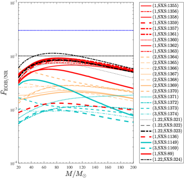
Figure 17: EOB/NR unfaithfulness for the $\ell=m=2$ mode computed over the eccentric SXS simulations publicly available using the model of Ref. Nagar et al. (2021b) with a more accurate computation of the Fourier transforms of both the EOB and NR waveforms. Comparing with Fig. 11 of Ref. Nagar et al. (2021b) one generally finds a better EOB/NR agreement for $M\lesssim 80M_{\odot}$.

Table 6: Maximum values $\bar{F}_{\rm EOB/NR}^{\rm max}$ of the unfaithfulness shown in Fig. 17. The third column of the table reports the lowest frequency used for integration, that approximately corresponds to the one of the second apastron of the NR waveform, so to cut the impact of the junk radiation.

$\#$	ID	$Mf_{\rm min}$	$\bar{F}_{\rm EOB/NR}^{\rm max}[\%]$
1	SXS:BBH:1355	0.0055	0.92
2	SXS:BBH:1356	0.0057	0.84
3	SXS:BBH:1358	0.006	0.91
4	SXS:BBH:1359	0.0055	0.82
5	SXS:BBH:1357	0.0055	0.82
6	SXS:BBH:1361	0.0055	0.90
7	SXS:BBH:1360	0.0055	0.86
8	SXS:BBH:1362	0.006	0.68
9	SXS:BBH:1363	0.006	0.75
10	SXS:BBH:1364	0.0055	0.3
11	SXS:BBH:1365	0.0055	0.28
12	SXS:BBH:1366	0.0055	0.28
13	SXS:BBH:1367	0.0055	0.23
14	SXS:BBH:1368	0.0058	0.32
15	SXS:BBH:1369	0.0056	0.21
16	SXS:BBH:1370	0.0055	0.58
17	SXS:BBH:1371	0.0054	0.19
18	SXS:BBH:1372	0.0055	0.11
19	SXS:BBH:1373	0.0055	0.17
20	SXS:BBH:1374	0.0055	0.10
21	SXS:BBH:89	0.00465	0.56
22	SXS:BBH:1136	0.0055	0.13
23	SXS:BBH:321	0.0055	0.73
24	SXS:BBH:322	0.0055	0.86
25	SXS:BBH:323	0.0055	0.83
26	SXS:BBH:324	0.0058	1.12
27	SXS:BBH:1149	0.0054	0.36
28	SXS:BBH:1169	0.004	0.099

As pointed out in Section IV of the main text, the EOB/NR unfaithfulness computation for eccentric inspirals is sensitive to the resolution of the Fourier transforms, that should be high enough to correctly resolve the low-frequency part of the (frequency-domain, FD) waveform. A FD resolution that is too low may eventually fictitiously worsen the $\bar{F}_{\rm EOB/NR}$ values for small mass binaries (say $M\simeq 60M_{\odot}$) binaries. This fact was unfortunately overlooked in previous works Chiaramello and Nagar (2020); Nagar et al. (2021b), and it now corrected in this Appendix.

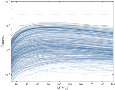
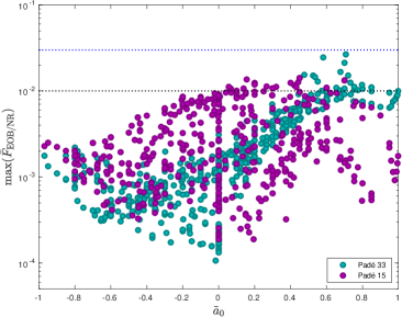
Figure 18: Left panel: unfaithfulness $\bar{F}_{\rm EOB/NR}(M)$ between the quasi-circular limit of the model presented in Ref. Nagar et al. (2021b) and the complete SXS catalog of noneccentric and nonprecessing (spin-aligned) waveforms. Roight panel: global picture of the maximum EOB/NR unfaithfulness using the best model presented in this paper (Padé 33, Fig. 7) and the one proposed in Ref. Nagar et al. (2021b) (Padé 15, corresponding to the left panel of this figure). The black and blue dotted lines mark the $0.01$ and $0.03$ values respectively. The model of Ref. Nagar et al. (2021b) is globally less NR faithful, but with a weak dependence on the effective spin parameter $\tilde{a}_{0}$. By contrast, the model used in this paper entails a very recognizable dependence on $\tilde{a}_{0}$.

We focus then on the, more advanced, model of Ref. Nagar et al. (2021b) and recomputed the $\bar{F}_{\rm EOB/NR}$ quantity by: (i) increasing the resolution of the Fourier transforms, obtained by suitably padding with zeros both the EOB and NR time-domain waveform; (ii) being careful to taper the EOB waveform so to have it visually consistent with the NR one and starting at approximately the same frequency, like the case shown in Fig. 16. Figure 17 is the updated version of Fig. 11 of Ref. Nagar et al. (2021b). Qualitatively, the two results are largely consistent with the old ones, although the more accurate calculation of the Fourier transforms generally determines and improved EOB/NR agreement for low values of $M$. In particular, it is interesting to note that for $M\sim 30M_{\odot}$ one has $3\times 10^{-3}\lesssim\bar{F}_{\rm EOB/NR}\lesssim 5\times 10^{-3}$ for $q=1$ nonspinning binaries (with any initial eccentricity), that is about half the corresponding values reported in Fig. 11 of Ref. Nagar et al. (2021b). A similar improvement is found for all other datasets, with the $\bar{F}_{\rm EOB/NR}$ curves that always mirror the improvement in resolving the FD inspiral part of the waveform. However, Fig. 17 also shows that BBH:SXS:324 remains somewhat an outlier, with the corresponding $\bar{F}_{\rm EOB/NR}$ value slightly above the $1\%$ level. Some complementary information is also found in Table 6, that reports the values of the maximal unfaithfulness $\bar{F}^{\rm max}_{\rm EOB/NR}$ together with the minimum values of the frequency $Mf_{\rm min}$ used in the calculation. For each dataset, these values approximately correspond to the frequency of the second apastron of the NR waveform and are always smaller than the frequency corresponding to the maximum of the amplitude of the Fourier transform, as typically illustrated in Fig. 16 for the SXS:BBH:1362 dataset.

A.2 Quasi-circular inspirals

In the spirit of providing a clear comparison between the results of Ref. Nagar et al. (2021b) and those discussed here, we also provide a new computation of $\bar{F}_{\rm EOB/NR}$ over the full SXS catalog of spin-aligned quasi-circular NR simulations using the model of. Nagar et al. (2021b) , analogously to what shown in Figs. 7 and 10 in the main text. The result is shown in the left panel of Fig. 18, where we can see that the $\bar{F}^{\rm max}_{\rm EOB/NR}$ is mostly below $10^{-2}$, with only a few some outliers that are in any case well below $0.03$. This results complements and updates the left panel of Fig. 3 of Ref. Nagar et al. (2021b) that was considering, for simplicity, only a reduced, though significant, sample of the full SXS catalog of 534 spin-aligned waveforms. A clearer comparison with the model proposed in this paper, in particular Fig. 7, is shown in the right panel of Fig. 7, that contrasts the two values of $\bar{F}^{\rm max}_{\rm EOB/NR}$ versus the effective spin $\tilde{a}_{0}$ for all datasets available.

References

- Chiaramello and Nagar (2020) D. Chiaramello and A. Nagar, Phys. Rev. D 101, 101501 (2020), eprint 2001.11736.
- Nagar et al. (2021a) A. Nagar, P. Rettegno, R. Gamba, and S. Bernuzzi, Phys. Rev. D 103, 064013 (2021a), eprint 2009.12857.
- Islam et al. (2021) T. Islam, V. Varma, J. Lodman, S. E. Field, G. Khanna, M. A. Scheel, H. P. Pfeiffer, D. Gerosa, and L. E. Kidder (2021), eprint 2101.11798.
- Nagar et al. (2021b) A. Nagar, A. Bonino, and P. Rettegno, Phys. Rev. D 103, 104021 (2021b), eprint 2101.08624.
- Albanesi et al. (2021) S. Albanesi, A. Nagar, and S. Bernuzzi, Phys. Rev. D 104, 024067 (2021), eprint 2104.10559.
- Liu et al. (2021) X. Liu, Z. Cao, and Z.-H. Zhu (2021), eprint 2102.08614.
- Khalil et al. (2021) M. Khalil, A. Buonanno, J. Steinhoff, and J. Vines, Phys. Rev. D 104, 024046 (2021), eprint 2104.11705.
- Nagar et al. (2020) A. Nagar, G. Riemenschneider, G. Pratten, P. Rettegno, and F. Messina, Phys. Rev. D 102, 024077 (2020), eprint 2001.09082.
- Riemenschneider et al. (2021) G. Riemenschneider, P. Rettegno, M. Breschi, A. Albertini, R. Gamba, S. Bernuzzi, and A. Nagar (2021), eprint 2104.07533.
- East et al. (2013) W. E. East, S. T. McWilliams, J. Levin, and F. Pretorius, Phys. Rev. D87, 043004 (2013), eprint 1212.0837.
- Gold and Brügmann (2013) R. Gold and B. Brügmann, Phys. Rev. D88, 064051 (2013), eprint 1209.4085.
- Cao and Han (2017) Z. Cao and W.-B. Han, Phys. Rev. D96, 044028 (2017), eprint 1708.00166.
- Liu et al. (2019) X. Liu, Z. Cao, and L. Shao (2019), eprint 1910.00784.
- Yun et al. (2021) Q. Yun, W.-B. Han, X. Zhong, and C. A. Benavides-Gallego, Phys. Rev. D 103, 124053 (2021), eprint 2104.03789.
- Abbott et al. (2020a) R. Abbott et al. (LIGO Scientific, Virgo), Phys. Rev. Lett. 125, 101102 (2020a), eprint 2009.01075.
- Abbott et al. (2020b) R. Abbott et al. (LIGO Scientific, Virgo), Astrophys. J. Lett. 900, L13 (2020b), eprint 2009.01190.
- Gamba et al. (2021) R. Gamba, M. Breschi, G. Carullo, P. Rettegno, S. Albanesi, S. Bernuzzi, and A. Nagar (2021), eprint 2106.05575.
- Bini et al. (2019) D. Bini, T. Damour, and A. Geralico, Phys. Rev. Lett. 123, 231104 (2019), eprint 1909.02375.
- Bini et al. (2020) D. Bini, T. Damour, and A. Geralico, Phys. Rev. D 102, 024062 (2020), eprint 2003.11891.
- Levi and Steinhoff (2016a) M. Levi and J. Steinhoff, JCAP 1601, 008 (2016a), eprint 1506.05794.
- Levi and Steinhoff (2016b) M. Levi and J. Steinhoff (2016b), eprint 1607.04252.
- Nagar et al. (2019a) A. Nagar, F. Messina, P. Rettegno, D. Bini, T. Damour, A. Geralico, S. Akcay, and S. Bernuzzi, Phys. Rev. D99, 044007 (2019a), eprint 1812.07923.
- Antonelli et al. (2020a) A. Antonelli, C. Kavanagh, M. Khalil, J. Steinhoff, and J. Vines, Phys. Rev. Lett. 125, 011103 (2020a), eprint 2003.11391.
- Antonelli et al. (2020b) A. Antonelli, C. Kavanagh, M. Khalil, J. Steinhoff, and J. Vines, Phys. Rev. D 102, 124024 (2020b), eprint 2010.02018.
- Damour and Nagar (2014) T. Damour and A. Nagar, Phys.Rev. D90, 044018 (2014), eprint 1406.6913.
- Nagar et al. (2018) A. Nagar et al., Phys. Rev. D98, 104052 (2018), eprint 1806.01772.
- Bini and Damour (2013) D. Bini and T. Damour, Phys.Rev. D87, 121501 (2013), eprint 1305.4884.
- Damour et al. (2014a) T. Damour, P. Jaranowski, and G. Schäfer, Phys. Rev. D89, 064058 (2014a), eprint 1401.4548.
- Damour et al. (2015) T. Damour, P. Jaranowski, and G. Schäfer, Phys. Rev. D91, 084024 (2015), eprint 1502.07245.
- Damour et al. (2016) T. Damour, P. Jaranowski, and G. Schäfer, Phys. Rev. D93, 084014 (2016), eprint 1601.01283.
- Nagar et al. (2019b) A. Nagar, G. Pratten, G. Riemenschneider, and R. Gamba (2019b), eprint 1904.09550.
- Bini and Damour (2012) D. Bini and T. Damour, Phys.Rev. D86, 124012 (2012), eprint 1210.2834.
- Damour et al. (2013) T. Damour, A. Nagar, and S. Bernuzzi, Phys.Rev. D87, 084035 (2013), eprint 1212.4357.
- (34) Updated Advanced LIGO sensitivity design curve, https://dcc.ligo.org/LIGO-T1800044/public.
- Husa et al. (2016) S. Husa, S. Khan, M. Hannam, M. Pürrer, F. Ohme, X. Jiménez Forteza, and A. Bohé, Phys. Rev. D93, 044006 (2016), eprint 1508.07250.
- Hinder et al. (2017) I. Hinder, L. E. Kidder, and H. P. Pfeiffer (2017), eprint 1709.02007.
- Damour et al. (2014b) T. Damour, F. Guercilena, I. Hinder, S. Hopper, A. Nagar, et al. (2014b), eprint 1402.7307.
- Rettegno et al. (2019) P. Rettegno, F. Martinetti, A. Nagar, D. Bini, G. Riemenschneider, and T. Damour (2019), eprint 1911.10818.