An estimate of approximation
of an analytic function of a matrix
by a rational function

Abstract.

Let $A$ be a square complex matrix; $z_{1}$, …, $z_{N}\in\mathbb{C}$ be arbitrary (possibly repetitive) points of interpolation; $f$ be an analytic function defined on a neighborhood of the convex hull of the union of the spectrum $\sigma(A)$ of the matrix $A$ and the points $z_{1}$, …, $z_{N}$; and the rational function $r=\frac{u}{v}$ (with the degree of the numerator $u$ less than $N$) interpolates $f$ at these points (counted according to their multiplicities). Under these assumptions estimates of the kind

$$\bigl{\lVert}f(A)-r(A)\bigr{\rVert}\leq\max_{\begin{subarray}{c}t\in[0,1]\\ \mu\in\operatorname{co}\{z_{1},z_{2},\dots,z_{N}\}\end{subarray}}\biggl{\lVert}\Omega(A)[v(A)]^{-1}\frac{\bigl{(}vf\bigr{)}^{{(N)}}\bigl{(}(1-t)\mu\mathbf{1}+tA\bigr{)}}{N!}\biggr{\rVert},$$

where $\Omega(z)=\prod_{k=1}^{N}(z-z_{k})$, are proposed. As an example illustrating the accuracy of such estimates, an approximation of the impulse response of a dynamic system obtained using the reduced-order Arnoldi method is considered, the actual accuracy of the approximation is compared with the estimate based on this paper.

Introduction

It is well-known [21, ch. IV, § 5] that the solution of the initial value problem $x^{\prime}(t)=Ax(t)$, $x(0)=x_{0}$, where $A$ is a square matrix, can be represented in the form $x(t)=e^{At}x_{0}$. Here $e^{At}$ is the result of the substitution of the matrix $A$ into the analytic function $\exp_{t}(\lambda)=e^{\lambda t}$. Some other analytic matrix functions arise in other applications [3, 7, 8, 9, 16, 22, 24, 26, 32].

As a rule, an analytic function of a matrix can be calculated only approximately. The usual way to approximately calculate an analytic function $f$ of a matrix $A$ is based on replacing $f$ with a polynomial or a rational function. The approximation by a rational function possesses some additional capabilities compared to a polynomial one: it can be more accurate and can approximate an analytic function on an unbounded set. In this paper, we propose estimates (Theorem 11 and its corollaries) of $f(A)-r(A)$, where $r$ is a rational function that interpolates $f$. Similar estimates for polynomial approximation were described in [27, 30].

As an application of these estimates, we consider the estimate of the accuracy of approximation of the impulse response of a dynamical system (9) using the Arnoldi reduced-order method (Theorems 22 and 24). The rational (Sections 6 and 7) reduced-order Arnoldi method is equivalent (Propostions 21 and 23) to the approximation of the analytic function $\exp_{t}(\lambda)=e^{\lambda t}$ by a rational function $r_{t}$. However, the function $r_{t}$ is not calculated explicitly.

In Section 8 we illustrate (Examples 1 and 2) our estimates of the Arnoldi reduced-order approximation using the properties of the numerical range. In Section 9, we describe a numerical experiment that shows the difference between our estimate and the actual approximation of the impulse response of a dynamical system obtained by means of the Arnoldi method.

In Sections 2 and 3, we recall some facts connected with polynomial and rational interpolation. Section 1 contains general notation. In Section 5, we recall the general properties of reduced-order methods.

1. Notation and other preliminaries

Let $n,m\in\mathbb{N}$. We denote by $\mathbb{C}^{n\times m}$ the space of all complex $n\times m$-matrices. We denote the identity matrix by the symbol $\mathbf{1}$ or $\mathbf{1}_{n\times n}$. The symbol $A^{H}$ means the conjugate transpose of $A\in\mathbb{C}^{n\times m}$. We represent elements $x\in\mathbb{C}^{n}$ as columns; thus the products $Ax$ and $y^{H}A$ make sense for $A\in\mathbb{C}^{n\times m}$, $x\in\mathbb{C}^{m}$, and $y\in\mathbb{C}^{n}$. Usually, we identify a matrix $A\in\mathbb{C}^{n\times m}$ and the operator $x\mapsto Ax$ from $\mathbb{C}^{m}$ to $\mathbb{C}^{n}$ induced by $A$. In particular, by the image of a matrix we mean the image of the operator induced by it.

We assume that the domains of analytic functions under consideration are open (maybe disconnected) subsets of $\mathbb{C}$.

Let $A\in\mathbb{C}^{n\times n}$. The spectrum of $A$ is the set $\sigma(A)=\{\lambda_{1},\lambda_{2},\dots,\lambda_{m}\}$ of all its eigenvalues. By the algebraic multiplicity of $\lambda_{j}$ we mean the multiplicity of $\lambda_{j}$ as the root of the characteristic polynomial.

Let the domain of an analytic function $f$ contain the spectrum of a matrix $A\in\mathbb{C}^{n\times n}$. The function $f$ applied to the matrix $A$ is the matrix

$$f(A)=\frac{1}{2\pi i}\int_{\Gamma}f(\lambda)R_{\lambda}\,d\lambda,$$

where the contour $\Gamma$ encloses the spectrum of $A$ and

$$R_{\lambda}=(\lambda\mathbf{1}-A)^{-1}$$

is the resolvent of $A$. The function

$$\exp_{t}(\lambda)=e^{\lambda t}$$

is the most important example of the function $f$ from the point of view of applications.

We denote by $\operatorname{co}M$ the convex hull of a set $M\subset\mathbb{C}$.

2. Polynomial interpolation

Let $z_{1},z_{2},\dots,z_{m}\in\mathbb{C}$ be given distinct points called points (or nodes) of interpolation and $n_{1},n_{2},\dots,n_{m}\in\mathbb{N}$ be their multiplicities. We set

$$N=\sum_{k=1}^{m}n_{k}.$$

Let $f$ be a function analytic in a neighborhood of the points of interpolation. The problem of polynomial interpolation is [15, 25, 36] is to find a polynomial $p$ of degree $\leq N-1$ satisfying the conditions

$$p^{(j)}(z_{k})=f^{(j)}(z_{k}),\qquad k=1,\dots,m;\;j=0,1,\dots,n_{k}-1.$$ (1)

Proposition 1 ([36, § 3.1, Theorem 2]).

Interpolation problem (1) has a unique solution.

Theorem 2 ([22, p. 5]).

Let $A\in\mathbb{C}^{n\times n}$. Let the spectrum $\sigma(A)$ of $A$ consists of the points $\lambda_{1},\lambda_{2},\dots,\lambda_{m}$, and let $w_{1},w_{2},\dots,w_{m}$ be their algebraic multiplicities. Let the functions $f$ and $p$ be analytic in a neighborhood of $\sigma(A)$. Let the functions $f$ and $p$ and their derivatives coincide at $\lambda_{i}$ up to the order $w_{i}-1$:

$$p^{(j)}(\lambda_{k})=f^{(j)}(\lambda_{k}),\qquad k=1,2,\dots,m;\;j=0,1,\dots,w_{m}-1.$$

Then $f(A)=p(A)$.

Theorem 3 ([36, § 3.1]).

Let $p$ be the interpolation polynomial satisfying (1) and a contour $\Gamma$ encloses the interpolation points $z_{1}$, $z_{2}$, …, $z_{m}$. Then at all points $z$ lying inside the contour $\Gamma$ one has

$$p(z) =\frac{1}{2\pi i}\int_{\Gamma}\frac{\Omega(\lambda)-\Omega(z)}{\Omega(\lambda)(\lambda-z)}f(\lambda)\,d\lambda,$$ (2)

$$f(z)-p(z) =\Omega(z)\frac{1}{2\pi i}\int_{\Gamma}\frac{f(\lambda)\,d\lambda}{\Omega(\lambda)(\lambda-z)},$$ (3)

where

$$\Omega(z)=\prod_{k=1}^{m}(z-z_{k})^{n_{k}}.$$

Sometimes it is convenient to specify the multiplicities of points of interpolation implicitly. Let $z_{1},z_{2},\dots,z_{N}\in\mathbb{C}$ be a list of points of interpolation (some of them may be repeated). We define the multiplicities of the points $z_{1}$, $z_{2}$, …, $z_{N}$ as the number of their repetition in this list.

Let a complex-valued function $f$ be defined and analytic in a neighborhood of the points $z_{1}$, $z_{2}$, …, $z_{N}$. The divided differences of the function $f$ with respect to the points $z_{1}$, $z_{2}$, …, $z_{N}$ are defined [12, 15, 25] by the recurrent relations

$$\begin{split}f[z_{i}]&=f(z_{i}),\qquad\qquad\qquad\qquad\qquad\qquad\qquad 1\leq i\leq N,\\ f[z_{i},z_{i+1}])&=\frac{f[z_{i+1}]-f[z_{i}]}{z_{i+1}-z_{i}},\qquad\qquad\qquad\qquad\qquad 1\leq i\leq N-1,\\ f[z_{i},\dots,z_{i+m}]&=\frac{f[z_{i+1},\dots,z_{i+m}]-f[z_{i},\dots,z_{i+m-1}]}{z_{i+m}-z_{i}},\quad 1\leq i\leq N-m.\end{split}$$ (4)

In these formulae, if the denominator vanishes, then the quotient is understood as the limit as $z_{i+m}-z_{i}\to 0$; the limit always exists and coincides with the derivative with respect to one of the arguments of the previous divided difference.

Proposition 4 ([12, formula (52)]).

Let a function $f$ be analytic in a neighborhood of the convex hull of the points $z_{1}$, $z_{2}$, …, $z_{N}$ (not necessarily different). Then

$$f[z_{1},z_{2},\dots,z_{N}]=\int_{0}^{1}\int_{0}^{t_{1}}\dots\int_{0}^{t_{N-2}}f^{{(N-1)}}\bigl{(}z_{1}+(z_{2}-z_{1})t_{1}+\dots{\\ }\dots+(z_{N-1}-z_{N-2})t_{N-2}+(z_{N}-z_{N-1})t_{N-1}\bigr{)}\,dt_{N-1}\dots dt_{1}.$$

Theorem 5 ([12, formula (51)], [14, formula (54)]).

Let a contour $\Gamma$ enclose the interpolation points $z_{1}$, $z_{2}$, …, $z_{N}$ (counted according to their multiplicities) and the function $f$ be analytic in a neighborhood of the domain surrounded by $\Gamma$. Then

$$f[z_{1},z_{2},\dots,z_{N}]=\frac{1}{2\pi i}\int_{\Gamma}\frac{f(\lambda)}{\Omega(\lambda)}\,d\lambda,$$

where

$$\Omega(z)=\prod_{i=1}^{N}(z-z_{i}).$$

Proposition 6 ([14, formula (52)]).

Let $f$ be an analytic function defined on an open set containing the interpolation points $z_{1}$, $z_{2}$, …, $z_{N}$ (counted according to their multiplicities). Let a polynomial $p$ of degree $\leq N-1$ satisfy interpolation conditions (1). Then for all $z$ from the domain of definition of $f$ one has

$$f(z)-p(z)=\Omega(z)\,f[z_{1},z_{2},\dots,z_{N},z].$$

Proof.

The proof follows from Theorems 3 and 5. ∎

3. Rational interpolation

A rational function is a function $r$ of a complex variable that can be represented in the form

$$r(z)=\frac{u(z)}{v(z)}=\frac{a_{0}+a_{1}z+\dots+a_{L}z^{L}}{b_{0}+b_{1}z+\dots+b_{M}z^{M}},$$

where $u$ and $v$ are polynomials. We call the pair $[L/M]$ the degree of $r$.

Let $z_{1},z_{2},\dots,z_{m}\in\mathbb{C}$ be given distinct points called points (or nodes) of interpolation and $n_{1},n_{2},\dots,n_{m}\in\mathbb{N}$ be their multiplicities. Let $f$ be an analytic function defined on a neighbourhood of the points of interpolation. The problem of rational interpolation is [4, 36] the problem of finding a rational function $r$ of degree $[L/M]$ or less satisfying the conditions

$$r^{(j)}(z_{k})=f^{(j)}(z_{k}),\qquad k=1,\dots,m;\;j=0,1,\dots,n_{k}-1.$$ (5)

Thus (5) consists of

$$N=\sum_{k=1}^{m}n_{k}$$

conditions. Usually it is assumed that $L+M\leq N-1$. It is also often assumed that the denominator $v$ is given. In the latter case, it is reasonable to assume that $L\leq N-1$. If $v(z)\equiv 1$, the problem of the rational interpolation is reduced to the polynomial one.

Proposition 7.

Let the points of interpolation $z_{1}$, $z_{2}$, …, $z_{m}$ have multiplicities $n_{1}$ $n_{2}$, …, $n_{m}$. Let $u$, $v$, and $f$ be analytic functions defined on a neighborhood of the points $z_{1}$, $z_{2}$, …, $z_{m}$; $v(z_{k})\neq 0$, $k=1,2,\dots,m$. Then the interpolation conditions

$$\Bigl{(}\frac{u}{v}\Bigr{)}^{(j)}(z_{k})=f^{(j)}(z_{k}),\qquad k=1,\dots,m;\;j=0,1,\dots,n_{k}-1,$$ (6)

are equivalent to the interpolation conditions

$$u^{(j)}(z_{k})=(vf)^{(j)}(z_{k}),\qquad k=1,\dots,m;\;j=0,1,\dots,n_{k}-1.$$ (7)

Proof.

Let conditions (6) be satisfied. Then for all $m=0,1,\dots,n_{k}-1$ we have (the argument $z_{k}$ is omitted for brevity)

$$u^{(m)}=\Bigl{(}\frac{u}{v}\cdot v\Bigr{)}^{(m)}=\sum_{j=0}^{m}\binom{m}{j}\Bigl{(}\dfrac{u}{v}\Bigr{)}^{(j)}v^{(m-j)}=\sum_{j=0}^{m}\binom{m}{j}(f)^{(j)}v^{(m-j)}=(vf)^{(m)}.$$

Conversely, let conditions (7) be satisfied. Then for all $m=0,1,\dots,n_{k}-1$ we have (the argument $z_{k}$ is again omitted for brevity)

$$\Bigl{(}\frac{u}{v}\Bigr{)}^{(m)} =(uv^{-1})^{(m)}=\sum_{j=0}^{m}\binom{m}{j}u^{(j)}(v^{-1})^{(m-j)}=\sum_{j=0}^{m}\binom{m}{j}(vf)^{(j)}(v^{-1})^{(m-j)}$$

$$=\bigl{[}(vf)v^{-1}\bigr{]}^{(m)}=f^{(m)}.\qed$$

Corollary 8.

Let the points of interpolation $z_{1}$, $z_{2}$, …, $z_{m}$ have multiplicities $n_{1}$ $n_{2}$, …, $n_{m}$. Let $N=\sum_{k=1}^{m}n_{k}$. Let $f$ be an analytic function defined on a neighborhood of the points $z_{1}$, $z_{2}$, …, $z_{m}$. Let $v$ be a given polynomial such that $v(z_{k})\neq 0$, $k=1,2,\dots,m$. Then there exists a unique polynomial $u$ of degree $L\leq N-1$ such that the rational function $r=\frac{u}{v}$ satisfies interpolation conditions (5).

Proof.

By Proposition 7, it is enough to show that there exists a polynomial $u$ that interpolates the function $vf$. By Proposition 1, this problem has a unique solution. ∎

Proposition 9.

Let $f$ be an analytic function defined on an open set $U$ containing the points of interpolation $z_{1}$, $z_{2}$, …, $z_{N}$ (not necessarily different). Let a rational function $r=\frac{u}{v}$ of degree $[L/M]$ satisfy interpolation conditions (5), $L\leq N-1$, and $v(z_{k})\neq 0$, $k=1,2,\dots,N$. Then for all $z\in U$ such that $v(z)\neq 0$ one has

$$f(z)-r(z)=\frac{\Omega(z)}{v(z)}\,\bigl{(}vf\bigr{)}[z_{1},z_{2},\dots,z_{N},z],$$

where

$$\Omega(z)=\prod_{k=1}^{N}(z-z_{k}).$$

Proof.

By Proposition 7, the polynomial $u$ interpolates the function $vf$. Therefore, by Proposition 6,

$$v(z)f(z)-u(z)=\Omega(z)\bigl{(}vf\bigr{)}[z,z_{1},z_{2},\dots,z_{N},z].$$

Hence

$$f(z)-\frac{u(z)}{v(z)}=\frac{\Omega(z)}{v(z)}\bigl{(}vf\bigr{)}[z,z_{1},z_{2},\dots,z_{N},z].\qed$$

4. The estimate

In this section, we present our estimate and its variants.

Theorem 10.

Let $A\in\mathbb{C}^{n\times n}$; $z_{1}$, $z_{2}$, …, $z_{N}\in\mathbb{C}$ be arbitrary (possibly repetitive) points of interpolation; $f$ be an analytic function defined on a neighborhood of the convex hull of the union of the spectrum $\sigma(A)$ of the matrix $A$ and the points $z_{1}$, $z_{2}$, …, $z_{N}$; a rational function $r=\frac{u}{v}$ of degree $[L/M]$ satisfy interpolation conditions (5); $L\leq N-1$; $v(z_{k})\neq 0$, $k=1,2,\dots,N$, and $v(\lambda)\neq 0$ for $\lambda\in\sigma(A)$. Then

$$f(A)-r(A)=\Omega(A)[v(A)]^{-1}\int_{0}^{1}\int_{0}^{t_{1}}\dots\int_{0}^{t_{N-1}}\bigl{(}vf\bigr{)}^{{(N)}}\bigl{(}(1-t_{1})z_{1}\mathbf{1}\\ +(t_{1}-t_{2})z_{2}\mathbf{1}+\dots+(t_{N-1}-t_{N})z_{N}\mathbf{1}+t_{N}A\bigr{)}\,dt_{N}dt_{N-1}\dots dt_{1},$$

where

$$\Omega(z)=\prod_{k=1}^{N}(z-z_{k}).$$

Proof.

By Proposition 9,

$$f(z)-r(z)=\frac{\Omega(z)}{v(z)}\,\bigl{(}vf\bigr{)}[z_{1},z_{2},\dots,z_{N},z].$$

On the other hand, by Proposition 4,

$$\bigl{(}vf\bigr{)}[z_{1},z_{2},\dots,z_{N},z]=\int_{0}^{1}\int_{0}^{t_{1}}\dots\int_{0}^{t_{N-1}}\bigl{(}vf\bigr{)}^{{(N)}}\bigl{(}z_{1}+(z_{2}-z_{1})t_{1}+\dots{\\ }+(z_{N}-z_{N-1})t_{N-1}+(z-z_{N})t_{N}\bigr{)}\,dt_{N}dt_{N-1}\dots dt_{1}.$$

Or

$$\bigl{(}vf\bigr{)}[z_{1},z_{2},\dots,z_{N},z]=\int_{0}^{1}\int_{0}^{t_{1}}\dots\int_{0}^{t_{N-1}}\bigl{(}vf\bigr{)}^{{(N)}}\bigl{(}(1-t_{1})z_{1}\\ +(t_{1}-t_{2})z_{2}+\dots+(t_{N-1}-t_{N})z_{N}+t_{N}z\bigr{)}\,dt_{N}dt_{N-1}\dots dt_{1}.$$

Therefore

$$f(A)-r(A)=\Omega(A)[v(A)]^{-1}\int_{0}^{1}\int_{0}^{t_{1}}\dots\int_{0}^{t_{N-1}}\bigl{(}vf\bigr{)}^{{(N)}}\bigl{(}(1-t_{1})z_{1}\mathbf{1}\\ +(t_{1}-t_{2})z_{2}\mathbf{1}+\dots+(t_{N-1}-t_{N})z_{N}\mathbf{1}+t_{N}A\bigr{)}\,dt_{N}dt_{N-1}\dots dt_{1}.\qed$$

Theorem 11.

Under assumptions of Theorem 10 for any linear functional $\xi$ on the linear space $\mathbb{C}^{n\times n}$ of matrices, one has

$$\bigl{|}\xi\bigl{[}f(A)-r(A)\bigr{]}\bigr{|}\leq\max_{\begin{subarray}{c}t\in[0,1]\\ \mu\in\operatorname{co}\{z_{1},z_{2},\dots,z_{N}\}\end{subarray}}\biggl{|}\xi\biggl{[}\Omega(A)[v(A)]^{-1}\frac{\bigl{(}vf\bigr{)}^{{(N)}}\bigl{(}(1-t)\mu\mathbf{1}+tA\bigr{)}}{N!}\biggr{]}\biggr{|}.\qed$$

Remark 1.

The matrix $v(A)$ (as any other polynomial of a matrix) is often badly conditioned. Therefore, a direct calculation of $[v(A)]^{-1}$ can be numerically unstable. To overcome this problem, one can first calculate the partial fraction decomposition of $\lambda\mapsto\Omega(\lambda)/v(\lambda)$ and then substitute $A$ in it.

Proof.

From Theorem 10 it follows that

$$\begin{split}\bigl{|}\xi\bigl{[}f(A)&-r(A)\bigr{]}\bigr{|}=\biggl{|}\xi\biggl{(}\int_{0}^{1}\int_{0}^{t_{1}}\dots\int_{0}^{t_{N-1}}\Omega(A)[v(A)]^{-1}\bigl{(}vf\bigr{)}^{{(N)}}\bigl{(}(1-t_{1})z_{1}\mathbf{1}+\dots\\ &+(t_{N-1}-t_{N})z_{N}\mathbf{1}+t_{N}A\bigr{)}\,dt_{N}dt_{N-1}\dots dt_{1}\biggr{)}\biggr{|}\\ &=\biggl{|}\int_{0}^{1}\int_{0}^{t_{1}}\dots\int_{0}^{t_{N-1}}\xi\bigl{[}\Omega(A)[v(A)]^{-1}\bigl{(}vf\bigr{)}^{{(N)}}\bigl{(}(1-t_{1})z_{1}\mathbf{1}+\dots\\ &+(t_{N-1}-t_{N})z_{N}\mathbf{1}+t_{N}A\bigr{)}\bigr{]}\,dt_{N}dt_{N-1}\dots dt_{1}\biggr{|}\\ &\leq\int_{0}^{1}\int_{0}^{t_{1}}\dots\int_{0}^{t_{N-1}}\max_{t_{1},\dots,t_{N}}\Bigl{|}\xi\Bigl{[}\Omega(A)[v(A)]^{-1}\bigl{(}vf\bigr{)}^{{(N)}}\bigl{(}(1-t_{1})z_{1}\mathbf{1}+\dots\\ &+(t_{N-1}-t_{N})z_{N}\mathbf{1}+t_{N}A\bigr{)}\Bigr{]}\Bigr{|}\,dt_{N}dt_{N-1}\dots dt_{1}.\end{split}$$ (8)

It is easy to see that the complex number

$$\frac{1}{1-t_{N}}\bigl{(}(1-t_{1})z_{1}+(t_{1}-t_{2})z_{2}+\dots+(t_{N-1}-t_{N})z_{N}\bigr{)}$$

runs over the convex hull $\operatorname{co}\{z_{1},z_{2},\dots,z_{N}\}$, and

$$\int_{0}^{1}\int_{0}^{t_{1}}\dots\int_{0}^{t_{N-1}}\,dt_{N}\dots dt_{1}=\frac{1}{N!}.$$

Therefore estimate (8) implies that

$$\bigl{|}\xi\bigl{[}f(A)-r(A)\bigr{]}\bigr{|}\leq\max_{\begin{subarray}{c}t\in[0,1]\\ \mu\in\operatorname{co}\{z_{1},z_{2},\dots,z_{N}\}\end{subarray}}\biggl{|}\xi\biggl{[}\Omega(A)[v(A)]^{-1}\frac{\bigl{(}vf\bigr{)}^{{(N)}}\bigl{(}(1-t)\mu\mathbf{1}+tA\bigr{)}}{N!}\biggr{]}\biggr{|}.\qed$$

Corollary 12.

Under assumptions of Theorem 10 for any $b,d\in\mathbb{C}^{n}$,

$$\bigl{|}d^{H}(f(A)-r(A))b\bigr{|}\\ \leq\max_{\begin{subarray}{c}t\in[0,1]\\ \mu\in\operatorname{co}\{z_{1},z_{2},\dots,z_{N}\}\end{subarray}}\biggl{|}d^{H}\biggl{[}\Omega(A)[v(A)]^{-1}\frac{\bigl{(}vf\bigr{)}^{{(N)}}\bigl{(}(1-t)\mu\mathbf{1}+tA\bigr{)}}{N!}\biggr{]}b\biggr{|}.$$

Proof.

It suffices to observe that the rule $A\mapsto d^{H}Ab$ is a linear functional on the space of matrices and refer to Theorem 11. ∎

Corollary 13.

Under assumptions of Theorem 10 for any $b\in\mathbb{C}^{n}$ (and the Euclidian norm $\lVert\cdot\rVert_{2}$ on $\mathbb{C}^{n}$),

$$\bigl{\lVert}\bigl{(}f(A)-r(A)\bigr{)}b\bigr{\rVert}_{2}\leq\max_{\begin{subarray}{c}t\in[0,1]\\ \mu\in\operatorname{co}\{z_{1},z_{2},\dots,z_{N}\}\end{subarray}}\biggl{\lVert}\Omega(A)[v(A)]^{-1}\frac{\bigl{(}vf\bigr{)}^{{(N)}}\bigl{(}(1-t)\mu\mathbf{1}+tA\bigr{)}}{N!}b\biggr{\rVert}_{2}.$$

Proof.

If $\bigl{(}f(A)-r(A)\bigr{)}b=0$ the proof is evident. If $\bigl{(}f(A)-r(A)\bigr{)}b\neq 0$, we set $d=\bigl{(}f(A)-r(A)\bigr{)}b\big{/}\lVert\bigl{(}f(A)-r(A)\bigr{)}b\rVert_{2}$. After that we refer to Corollary 12. ∎

Corollary 14.

Under assumptions of Theorem 10 (for any norm on the space of matrices),

$$\bigl{\lVert}f(A)-r(A)\bigr{\rVert}\leq\max_{\begin{subarray}{c}t\in[0,1]\\ \mu\in\operatorname{co}\{z_{1},z_{2},\dots,z_{N}\}\end{subarray}}\biggl{\lVert}\Omega(A)[v(A)]^{-1}\frac{\bigl{(}vf\bigr{)}^{{(N)}}\bigl{(}(1-t)\mu\mathbf{1}+tA\bigr{)}}{N!}\biggr{\rVert}.$$

Proof.

Let $\xi$ be a linear functional on the space of matrices (equipped by an arbitrary norm) such that $\lVert\xi\rVert=1$ and

$$\lVert f(A)-r(A)\rVert=\xi\bigl{(}f(A)-r(A)\bigr{)}.$$

Such a functional exists by the Hahn–Banach theorem [23, Theorem 2.7.4]. Then from Theorem 11 we have

$$\lVert f(A) -r(A)\rVert=\xi\bigl{[}f(A)-r(A)\bigr{]}=\bigl{|}\xi\bigl{[}f(A)-r(A)\bigr{]}\bigr{|}$$

$$\leq\max_{\begin{subarray}{c}t\in[0,1]\\ \mu\in\operatorname{co}\{z_{1},z_{2},\dots,z_{N}\}\end{subarray}}\Bigl{|}\xi\bigl{[}\Omega(A)[v(A)]^{-1}\frac{\bigl{(}vf\bigr{)}^{{(N)}}\bigl{(}(1-t)\mu\mathbf{1}+tA\bigr{)}}{N!}\bigr{]}\Bigr{|}$$

$$\leq\max_{\begin{subarray}{c}t\in[0,1]\\ \mu\in\operatorname{co}\{z_{1},z_{2},\dots,z_{N}\}\end{subarray}}\Bigl{\lVert}\Omega(A)[v(A)]^{-1}\frac{\bigl{(}vf\bigr{)}^{{(N)}}\bigl{(}(1-t)\mu\mathbf{1}+tA\bigr{)}}{N!}\Bigr{\rVert}.\qed$$

Corollary 15.

Let a function $f$ be analytic on an open circle of radius $r$ centered at a point $z_{0}$ and the spectrum of a square matrix $A$ be contained in this circle. Then the difference between the exact value $f(A)$ and the Padé approximant $r=\frac{u}{v}$ of degree $[L/M]$ of the function $f$ at the point $z_{0}$ applied to $A$ admits the estimate

$$\bigl{\|}f(A)-r(A)\bigr{\|}\leq\max_{t\in[0,1]}\Bigl{\lVert}(A-z_{0}\mathbf{1})^{N}[v(A)]^{-1}\frac{\bigl{(}vf\bigr{)}^{(N)}\bigl{(}(1-t)z_{0}\mathbf{1}+tA\bigr{)}}{N!}\Bigr{\rVert},$$

where $N=L+M+1$. It is assumed that $v(\lambda)\neq 0$ for $\lambda\in\sigma(A)$.

Proof.

It suffices to recall that the Padé approximant is an interpolation rational function that corresponds to a single interpolation point $z_{0}$ of multiplicity $N$. ∎

An analogue of Corollary 15 for approximation by the Taylor polynomials is established in [30].

5. Reduced-order methods

In this Section, we describe an application of Corollary 12 for accuracy of approximation of the impulse response of a single-input, single-output dynamical system [1] based on the Arnoldi type method of order reduction.

We consider a dynamical system [1, 31] with the input $u$ and the output $y$ governed by the equations

$$\begin{split}x^{\prime}(t)&=Ax(t)+bu(t),\\ y(t)&=d^{H}x(t),\end{split}$$ (9)

where $A\in\mathbb{C}^{n\times n}$ and $b,d\in\mathbb{C}^{n}$ are given matrices. The following fact is well known.

Theorem 16 ([1, p. 65], [38, p. 46]).

The solution of problem (9) satisfying the initial condition

$$x(t_{0})=x_{0}$$

can be represented as

$$y(t)=d^{H}\biggl{(}\exp_{t-t_{0}}(A)x_{0}+\int_{t_{0}}^{t}\exp_{t-r}(A)bu(r)\,dr\biggr{)},\qquad t\geq t_{0},$$

where $\exp_{t}(\lambda)=e^{\lambda t}$.

This formula shows that the principal part of solving the problem (9) consists in finding the function $t\mapsto d^{H}\exp_{t}(A)b$. We call the function $t\mapsto d^{H}\exp_{t}(A)b$ the (scalar) impulse response and we call the function $t\mapsto\exp_{t}(A)b$ the (vector) impulse response.

A system of reduced order with respect to (9) is [1, 17, 34] the system governed by the equations

$$\begin{split}\hat{x}^{\prime}(t)&=\widehat{A}\hat{x}(t)+\hat{b}u(t),\\ \hat{y}(t)&=\hat{d}^{H}\hat{x}(t),\end{split}$$ (10)

in which the order $\hat{n}$ of the matrix $\widehat{A}$ is substantially less than the order $n$ of the matrix $A$, but the output $\hat{y}$ is close to the output $y$ of problem (9).

We say that problem (10) is constructed by a projection method if the coefficients $\widehat{A},\hat{b},\hat{d}$ in (10) are expressed in terms of the coefficients of initial problem (9) by the formulae

$$\widehat{A}=\Lambda AV,\qquad\hat{b}=\Lambda b,\qquad\hat{d}=Vd,$$ (11)

where $V\in\mathbb{C}^{n\times\hat{n}}$ and $\Lambda\in\mathbb{C}^{\hat{n}\times n}$ are some matrices.

We will always assume that the following normalizing assumption is fulfilled:

$$\begin{split}\Lambda V&=\mathbf{1}_{\hat{n}\times\hat{n}},\end{split}$$ (12)

where $\mathbf{1}_{\hat{n}\times\hat{n}}$ is the identity matrix of the size $\hat{n}\times\hat{n}$. Moreover, usually we will assume that condition (14) from the following proposition is fulfilled.

Proposition 17.

Let $S\in\mathbb{C}^{\hat{n}\times\hat{n}}$ be an arbitrary invertible matrix. We set $V_{1}=VS$, $\Lambda_{1}=S^{-1}\Lambda$,

$$\widehat{A}_{1}=\Lambda_{1}AV_{1},\qquad\hat{b}_{1}=\Lambda_{1}b,\qquad\hat{d}^{H}_{1}=d^{H}V_{1}.$$

Then the solution $\hat{y}$ of the problem

$$\begin{split}{\hat{x}}_{1}^{\prime}&=\widehat{A}_{1}{\hat{x}}_{1}+\hat{b}_{1}u(t),\\ \hat{y}(t)&=\hat{d}^{H}_{1}{\hat{x}}(t)\end{split}$$ (13)

coincides with the solution $\hat{y}$ of problem (10).

Proof.

We make the change ${\hat{x}}=S{\hat{x}}_{1}$ in problem (10):

$$\begin{split}S{\hat{x}}_{1}^{\prime}(t)&=\Lambda AVS{\hat{x}}_{1}(t)+\hat{b}u(t),\\ \hat{y}(t)&=\hat{d}^{H}S{\hat{x}}_{1}(t).\end{split}$$

We multiply the differential equation by $S^{-1}$ and use the equality $S^{-1}S=\mathbf{1}$:

$$\begin{split}{\hat{x}}_{1}^{\prime}(t)&=S^{-1}\Lambda AVS{\hat{x}}_{1}(t)+S^{-1}\hat{b}u(t),\\ \hat{y}(t)&=\hat{d}^{H}S{\hat{x}}_{1}(t).\end{split}$$

We rewrite these equations as

$$\begin{split}{\hat{x}}_{1}^{\prime}(t)&=\Lambda_{1}AV_{1}{\hat{x}}_{1}(t)+S^{-1}\Lambda bu(t),\\ \hat{y}(t)&=d^{H}VS{\hat{x}}_{1}(t),\end{split}$$

We have arrived at system (13). ∎

In connection with Proposition 17, the columns of the matrix $V$ and the rows of the matrix $\Lambda$ are usually taken orthonormal. This leads to the fact that calculations by the formula $\widehat{A}=\Lambda AV$ result in minimal round-off errors.

Proposition 18.

Let the columns of the matrix $V$ be orthonormalized and the matrix $\Lambda$ be defined by the formula

$$\Lambda=V^{H}.$$ (14)

Then assumption (12) is fulfilled, and the matrix $V\Lambda\in\mathbb{C}^{n\times n}$ defines an orthogonal projector $P$ onto the linear span of the columns of the matrix $V$.

Proof.

By (14), the matrix $\Lambda V$ is the Gram matrix of the columns of the matrix $V$. This observation implies the first statement.

We extend the set consisting of $\hat{n}$ columns of the matrix $V$ to an orthonormal basis of $\mathbb{C}^{n}$. We take an arbitrary vector $x\in\mathbb{C}^{n}$. By (14), the vector $\Lambda x$ consists of the first $n$ coordinates of $x$ in this basis. Therefore, the vector $V(\Lambda x)\in\mathbb{C}^{n}$ coincides with the projection of $x$ onto the linear span of the first $\hat{n}$ basis vectors. ∎

Corollary 19.

Under assumptions of Proposition 18 $AV-V\widehat{A}=(\mathbf{1}-P)AV$.

Proof.

Indeed, $AV-V\widehat{A}=AV-V\Lambda AV=(\mathbf{1}-P)AV$. ∎

It is clear that the fundamental part in the construction of reduced-order model (11) is the choice of matrices $V$ and $\Lambda$. Proposition 20 below shows that the solution $\hat{y}$ of the reduced-order problem (12) is determined by the linear span of the columns of the matrices $V$ and $\Lambda^{H}$.

6. Two-sided rational Arnoldi

We consider two variants of the Arnoldi method [1, 17, 22, 28, 33, 34, 35] of order reduction. We always assume that assumption (14) is fulfilled.

Let $\varkappa_{0}$ and $\chi_{0}$ be given nonnegative integers called multiplicities. Let the image of the operator $V$ contains the vectors

$$b,Ab,A^{2}b,\dots,A^{\varkappa_{0}-1}b,$$ (15)

and the image of the operator $\Lambda^{H}$ contains the vectors

$$d,A^{H}d,(A^{H})^{2}d,\dots,(A^{H})^{\chi_{0}-1}d.$$ (16)

Further, let $\lambda_{1},\lambda_{2},\dots,\lambda_{m}\in\mathbb{C}$ be points not lying in the spectrum of $A$, and $\varkappa_{1},\dots,\varkappa_{m}$ and $\chi_{1},\dots,\chi_{m}$ be nonnegative integers. We additionally assume that the image of the operator $V$ contains the vectors

$$\begin{split}(\lambda_{1}I-A)^{-1}b,\;&(\lambda_{1}I-A)^{-2}b,\;\dots,\;(\lambda_{1}I-A)^{-\varkappa_{1}}b,\\ \dots\dots\dots\dots\dots&\dots\dots\dots\dots\dots\dots\dots\dots\dots\dots\dots{\\ }(\lambda_{m}I-A)^{-1}b,\;&(\lambda_{m}I-A)^{-2}b,\;\dots,\;(\lambda_{m}I-A)^{-\varkappa_{m}}b\end{split}$$ (17)

and the image of the operator $\Lambda^{H}$ contains the vectors

$$\begin{split}(\bar{\lambda}_{1}I-A^{H})^{-1}d,\;&(\bar{\lambda}_{1}I-A^{H})^{-2}d,\;\dots,\;(\bar{\lambda}_{1}I-A^{H})^{-\chi_{1}}d,\\ \dots\dots\dots\dots\dots&\dots\dots\dots\dots\dots\dots\dots\dots\dots\dots\dots\dots{\\ }(\bar{\lambda}_{m}I-A^{H})^{-1}d,\;&(\bar{\lambda}_{m}I-A^{H})^{-2}d,\;\dots,\;(\bar{\lambda}_{m}I-A^{H})^{-\chi_{m}}d.\end{split}$$ (18)

It is convenient to interpret vectors (15) and (16) as analogues of vectors (17) and (18) corresponding to the point $\lambda_{0}=\infty$.

In two-sided Arnoldi methods, it is assumed that the image of $V=\Lambda^{H}$ is defined as the linear span of vectors (15)–(18). In one-sided Arnoldi methods, it is assumed that the image of $V=\Lambda^{H}$ is defined as the linear span of vectors (15) and (17) only. We assume that these vectors are linear independent. It is convenient to combine the verification of the linear independence with the orthonormal process. The columns of the matrix $V=\Lambda^{H}$ are usually taken orthonormal.

By Proposition 17, reduced-order system (10) is defined by the points $\lambda_{0}=\infty$, $\lambda_{1},\dots,\lambda_{m}\in\mathbb{C}$ and their multiplicities $\varkappa_{k}$ and $\chi_{k}$, $k=0,\dots,m$. The quality of approximation of system (9) by system (10) depends only of these parameters.

Proposition 20 ([13, Lemma 3.1], [19, Lemma 3.1]).

• Let $V\in\mathbb{C}^{n\times\hat{n}}$ and $\Lambda\in\mathbb{C}^{\hat{n}\times n}$ satisfy assumption (12). Let the image of the matrix $V$ contain vectors (15) and (17), and the image of the matrix $\Lambda^{H}$ contain vectors (16) and (18). We consider matrices (11). Let points $\lambda_{1}$, …, $\lambda_{m}\in\mathbb{C}$ be not both in the spectrum of $A$ and the spectrum of $\widehat{A}$. Then for any rational function $r$ of the form

  $$r(\lambda)=\sum_{k=1}^{m}\sum_{j=1}^{\varkappa_{k}+\chi_{k}}\frac{g_{jk}}{{(\lambda_{k}-\lambda)^{j}}}+\sum_{j=0}^{\varkappa_{0}+\chi_{0}-1}g_{j0}\lambda^{j}$$

  one has

  $$d^{H}r(A)\,b=\hat{d}^{H}r(\widehat{A})\,\hat{b}.$$

• Let $V\in\mathbb{C}^{n\times\hat{n}}$ satisfy assumption $V^{H}V=\mathbf{1}_{\hat{n}\times\hat{n}}$. Let the image of the matrix $V$ contain vectors (15) and (17). We consider matrices (11) with $\Lambda=V^{H}$. Let points $\lambda_{1}$, …, $\lambda_{m}\in\mathbb{C}$ be not both in the spectrum of $A$ and the spectrum of $\widehat{A}$. Then for any rational function $r$ of the form

  $$r(\lambda)=\sum_{k=1}^{m}\sum_{j=1}^{\varkappa_{k}}\frac{g_{jk}}{{(\lambda_{k}-\lambda)^{j}}}+\sum_{j=0}^{\varkappa_{0}-1}g_{j0}\lambda^{j}$$

  one has

  $$r(A)b=Vr(\widehat{A})\hat{b}.$$

Proposition 21 ([6]).

Let the image of the matrix $V$ contain vectors (15) and (17) and the image of the matrix $\Lambda^{H}$ contain vectors (16) and (18). Let $V\in\mathbb{C}^{n\times\hat{n}}$ and $\Lambda\in\mathbb{C}^{\hat{n}\times n}$ satisfy assumption (12). We consider matrices (11). Let $\sigma(\widehat{A})$ consist of the points $\hat{\mu}_{1},\dots,\hat{\mu}_{\hat{m}}\in\mathbb{C}$, and let $\hat{w}_{1},\dots,\hat{w}_{\hat{m}}$ be their algebraic multiplicities.

Let the points $\lambda_{1}$, …, $\lambda_{m}\in\mathbb{C}$ be not both in the spectrum of $A$ and the spectrum of $\widehat{A}$. Let a rational function $r_{t}$ of the form

$$r_{t}(\lambda)=\sum_{k=1}^{m}\sum_{j=1}^{\varkappa_{k}+\chi_{k}}\frac{g_{jk}(t)}{{(\lambda_{k}-\lambda)^{j}}}+\sum_{j=0}^{\varkappa_{0}+\chi_{0}-1}g_{j0}(t)\lambda^{j}$$ (19)

satisfy the following interpolation assumptions: the function $r_{t}$ coincides with the function $\exp_{t}(\lambda)=e^{\lambda t}$ at the points $\hat{\mu}_{1},\dots,\hat{\mu}_{\hat{m}}$ with the derivatives up to the orders $\hat{w}_{1}-1,\dots,\hat{w}_{\hat{m}}-1$:

$$r_{t}^{(j)}(\hat{\mu}_{k})=\exp_{t}^{(j)}(\hat{\mu}_{k}),\qquad k=1,2,\dots,\hat{m};\;j=0,1,\dots,w_{\hat{m}}-1.$$

Then one has

$$d^{H}r_{t}(A)b=\hat{d}^{H}\exp_{t}(\widehat{A})\hat{b},\qquad t\in\mathbb{R}.$$

Proof.

Since the function $r_{t}$ satisfies the interpolation conditions, by Theorem 2, we have $\exp_{t}(\widehat{A})=r_{t}(\widehat{A})$. Now from Proposition 20(a) it follows that $d^{H}r_{t}(A)b=\hat{d}^{H}r_{t}(\widehat{A})\hat{b}$. ∎

Theorem 22.

Let vectors (15), (16), (17), and (18) form a basis in the image of the matrix $V$, and let $V^{H}V=\mathbf{1}_{\hat{n}\times\hat{n}}$. Consider matrices (11) with $\Lambda=V^{H}$. Let $\sigma(\widehat{A})$ consists of the points $\hat{\mu}_{1},\dots,\hat{\mu}_{\hat{m}}\in\mathbb{C}$, and let $\hat{w}_{1},\dots,\hat{w}_{\hat{m}}$ be their algebraic multiplicities.

Let the points $\lambda_{1}$, …, $\lambda_{m}\in\mathbb{C}$ be not both in $\sigma(A)$ and in $\sigma(\widehat{A})$. Let the reduced-order system be defined by (10). Then the difference between scalar impulse responses of initial (9) and reduced-order (10) systems admits the estimate

$$\bigl{|}d^{H}\exp_{t}(A)b-\hat{d}^{H}\exp_{t}(\widehat{A})\hat{b}\bigr{|}\leq\\ \leq\max_{\begin{subarray}{c}s\in[0,1]\\ \mu\in\operatorname{co}\{\hat{\mu}_{1},\dots,\hat{\mu}_{\hat{m}}\}\end{subarray}}\biggl{|}d^{H}\Bigl{[}\Omega(A)[v(A)]^{-1}\frac{\bigl{(}v\exp_{t}\bigr{)}^{{(\hat{n})}}\bigl{(}(1-s)\mu\mathbf{1}+sA\bigr{)}}{\hat{n}!}\Bigr{]}b\biggr{|},$$

where

$$v(\lambda) =\sum_{k=1}^{m}(\lambda-\lambda_{k})^{\varkappa_{k}+\chi_{k}},$$

$$\Omega(\lambda) =\sum_{k=1}^{\hat{m}}(\lambda-\hat{\mu}_{k})^{\hat{\omega}_{k}}.$$

We note that under assumptions of Theorem 22

$$\hat{n}=\sum_{k=0}^{m}\varkappa_{k}+\chi_{k}=\sum_{k=1}^{\hat{m}}\hat{w}_{k}.$$

Proof.

By Proposition 21,

$$d^{H}\exp_{t}(A)\,b-\hat{d}^{H}\exp_{t}(\widehat{A})\,\hat{b}=d^{H}\bigl{(}\exp_{t}(A)-r_{t}(A)\bigr{)}\,b,$$

where $r_{t}$ is a function of the form (19) that interpolates the function $\exp_{t}(\lambda)=e^{\lambda t}$ at the points $\hat{\mu}_{1},\dots,\hat{\mu}_{\hat{m}}$ with multiplicities $\hat{w}_{1},\dots,\hat{w}_{\hat{m}}$.

It remains to apply Corollary 12, see also Theorem 10. The degree $L$ of the numerator of function (19) is less than or equal to $-1+\sum_{k=0}^{m}\varkappa_{k}+\chi_{k}$. Since the vectors (15), (16), (17), and (18) form a basis, the order $\hat{n}$ of the matrix $\widehat{A}$ (this order determines the number of interpolation conditions) equals $\sum_{k=0}^{m}\varkappa_{k}+\chi_{k}$. Therefore the assumption $L\leq\hat{n}-1$ from Theorem 10 is fulfilled. Furthermore, the denominator $v(\lambda)=\prod_{k=1}^{m}(\lambda-\lambda_{k})^{\varkappa_{k}+\chi_{k}}$ of function (19), by assumptions of Theorem 22, does not vanish both at the points of interpolation $\hat{\mu}_{k}$ and on $\sigma(A)$. Thus, all assumptions of Theorem 10 are fulfilled. ∎

7. One-sided rational Arnoldi

Theorem 24 below is an analogue of Theorem 22 for the approximation $t\mapsto Ve^{\widehat{A}t}\hat{b}$ of the vector impulse response $t\mapsto e^{At}b$. It corresponds to the one-sided Arnoldi method that allows one to calculate approximately the whole vector $e^{At}b$.

Proposition 23 ([19, Theorem 3.3]).

Let the image of the matrix $V$ contain vectors (15) and (17), and let $V^{H}V=\mathbf{1}_{\hat{n}\times\hat{n}}$. We consider matrices (11) with $\Lambda=V^{H}$. Let $\sigma(\widehat{A})$ consists of the points $\hat{\mu}_{1},\dots,\hat{\mu}_{\hat{m}}\in\mathbb{C}$, and let $\hat{w}_{1},\dots,\hat{w}_{\hat{m}}$ be their algebraic multiplicities.

Let the points $\lambda_{1}$, …, $\lambda_{m}\in\mathbb{C}$ be not both in $\sigma(A)$ and in $\sigma(\widehat{A})$. Let $f$ be an analytic function defined on a neighborhood of the union of $\sigma(A)$ and $\sigma(\widehat{A})$.

Let a rational function $r_{t}$ of the form

$$r_{t}(\lambda)=\sum_{k=1}^{m}\sum_{j=1}^{\varkappa_{k}}\frac{g_{jk}(t)}{{(\lambda_{k}-\lambda)^{j}}}+\sum_{j=0}^{\varkappa_{0}-1}g_{j0}(t)\lambda^{j}$$ (20)

satisfy the following interpolation assumptions: the function $r_{t}$ coincides with the function $\exp_{t}$ at all points $\hat{\mu}_{1},\dots,\hat{\mu}_{\hat{m}}$ of $\sigma(\widehat{A})$ with the derivatives up to the order $\hat{w}_{1}-1,\dots,\hat{w}_{\hat{m}}-1$:

$$r_{t}^{(j)}(\hat{\mu}_{k})=\exp_{t}^{(j)}(\hat{\mu}_{k}),\qquad k=1,2,\dots,\hat{m};\;j=0,1,\dots,\hat{w}_{\hat{m}}-1.$$

Then one has

$$r_{t}(A)\,b=V\exp_{t}(\widehat{A})\,\hat{b}.$$

Proof.

The proof is similar to that of Proposition 21. ∎

Theorem 24.

Let vectors (15) and (17) form a basis in the image of the matrix $V$, and $V^{H}V=\mathbf{1}_{\hat{n}\times\hat{n}}$. Consider matrices (11) with $\Lambda=V^{H}$. Let $\sigma(\widehat{A})$ consist of the points $\hat{\mu}_{1},\dots,\hat{\mu}_{\hat{m}}\in\mathbb{C}$, and let $\hat{w}_{1},\dots,\hat{w}_{\hat{m}}$ be their algebraic multiplicities.

Let the points $\lambda_{1}$, …, $\lambda_{m}\in\mathbb{C}$ be not both in $\sigma(A)$ and in $\sigma(\widehat{A})$. Let $f$ be an analytic function defined on a neighbourhood of the union of $\sigma(A)$ and $\sigma(\widehat{A})$. Then the difference between vector impulse responses of initial (9) and reduced-order (10) systems admits the estimate

$$\bigl{\lVert}\exp_{t}(A)b-V\exp_{t}(\widehat{A})\,\hat{b}\bigr{\rVert}\\ \leq\max_{\begin{subarray}{c}s\in[0,1]\\ \mu\in\operatorname{co}\{\hat{\mu}_{1},\dots,\hat{\mu}_{\hat{m}}\}\end{subarray}}\biggl{\lVert}\Omega(A)[v(A)]^{-1}\frac{\bigl{(}v\exp_{t}\bigr{)}^{{(\hat{n})}}\bigl{(}(1-s)\mu\mathbf{1}+sA\bigr{)}}{\hat{n}!}b\biggr{\rVert},$$ (21)

where

$$v(\lambda) =\sum_{k=1}^{m}(\lambda-\lambda_{k})^{\varkappa_{k}},$$

$$\Omega(\lambda) =\sum_{k=1}^{\hat{m}}(\lambda-\hat{\mu}_{k})^{\hat{\omega}_{k}}.$$

We note that under assumptions of Theorem 24

$$\hat{n}=\sum_{k=0}^{m}\varkappa_{k}=\sum_{k=1}^{\hat{m}}\hat{w}_{k}.$$

Proof.

The proof is similar to that of Theorem 22. By Proposition 23,

$$\exp_{t}(A)b-V\exp_{t}(\widehat{A})\hat{b}=\exp_{t}(A)b-r_{t}(A)\,b.$$

It remains to apply Corollary 13. ∎

8. Numerical range

In this section we describe (Examples 1 and 2) two cases when estimate (21) can be used effectively.

The numerical range of a matrix $A\in\mathbb{C}^{n\times n}$ is [18] the set

$$w(A)=\{\,\langle Az,z\rangle:\,\lVert z\rVert_{2}=1\,\}.$$

It is known [18, p. 4] that $w(A)$ is a closed convex subset of $\mathbb{C}$. The numerical range $w(A)$ of a normal matrix $A$ coincides [18, p. 16] with the convex hall of $\sigma(A)$.

Proposition 25.

The numerical range $w(A)$ possesses the following properties:

• $w(A)$ is a compact set;

• $w(A)$ is contained in the ball of radius $\lVert A\rVert_{2\to 2}$ centered at zero;

• $w(A)$ contains $\sigma(A)$;

• $w(\alpha A)=\alpha w(A)$, $\alpha\in\mathbb{C}$.

Proof.

Evident. ∎

Proposition 26.

Let the columns of the matrix $V\in\mathbb{C}^{n\times\hat{n}}$ be orthonormalized and assumption (14) be fulfilled. Then the numerical range $w(\widehat{A})$ and (consequently) the spectrum $\sigma(\widehat{A})$ of the matrix $\widehat{A}=\Lambda AV$ are contained in the numerical range $w(A)$ of the matrix $A$.

Proof.

First, we notice that under the assumptions of the proposition $\lVert V\varphi\rVert=\lVert\varphi\rVert$ for any $\varphi\in\mathbb{C}^{n}$. In fact, by (12) and Proposition 18,

$$\lVert V\varphi\rVert=\sqrt{\langle V\varphi,V\varphi\rangle}=\sqrt{\langle\Lambda V\varphi,\varphi\rangle}=\sqrt{\langle\varphi,\varphi\rangle}=\lVert\varphi\rVert.$$

Let $\varphi\in\mathbb{C}^{n}$ be an arbitrary vector such that $\lVert\varphi\rVert=1$. Then

$$\langle\widehat{A}\varphi,\varphi\rangle=\langle\Lambda AV\varphi,\varphi\rangle=\langle AV\varphi,V\varphi\rangle\in w(A),$$

because $\lVert V\varphi\rVert=1$. ∎

Example 1.

Let a matrix $A$ be self-adjoint and its spectrum be contained in a segment $[a,b]$. Hence, by Propositions 25 and 26, $\sigma(\widehat{A})\subseteq w(\widehat{A})\subseteq w(A)\subseteq[a,b]$. We recall that since a function $f(A)$ of a self-adjoint matrix $A$ is normal, the norm $\lVert f(A)\rVert$ coincides with the maximum of $|f(\lambda)|$ on the spectrum of $A$. Therefore the right-hand side of (21) can be estimated by

$$\max_{\begin{subarray}{c}s\in[0,1]\\ \lambda,\mu\in[a,b]\end{subarray}}\biggl{|}\Omega(\lambda)[v(\lambda)]^{-1}\frac{\bigl{(}v\exp_{t}\bigr{)}^{{(\hat{n})}}\bigl{(}(1-s)\mu+s\lambda\bigr{)}}{\hat{n}!}\biggr{|}\cdot\lVert b\rVert\\ =\max_{\lambda\in[a,b]}\biggl{|}\Omega(\lambda)[v(\lambda)]^{-1}\frac{\bigl{(}v\exp_{t}\bigr{)}^{{(\hat{n})}}(\lambda)}{\hat{n}!}\biggr{|}\cdot\lVert b\rVert.$$

We set [11, p. 11], [20, Theorem 10.5], [29] (clearly, the matrix $A+A^{H}$ is self-adjoint)

$$\mu(A)=\max\Bigl{\{}\lambda:\,\lambda\in\sigma\Bigl{(}\frac{A+A^{H}}{2}\Bigr{)}\Bigr{\}}.$$

The number $\mu(A)$ is called the logarithmic norm of $A$.

Proposition 27.

For any matrix $A\in\mathbb{C}^{n\times n}$ one has

$$\mu(A)=\max\{\,\operatorname{Re}\lambda:\,\lambda\in w(A)\,\}.$$

Proof.

Indeed,

$$\max\{\,\operatorname{Re}\lambda:\,\lambda\in w(A)\,\}=\max\{\,\operatorname{Re}\langle Az,z\rangle:\,\lVert z\rVert_{2}=1\,\}=\\ =\max\biggl{\{}\,\operatorname{Re}\Bigl{(}\Bigl{\langle}\frac{A+A^{H}}{2}z,z\Bigr{\rangle}+\Bigl{\langle}\frac{A-A^{H}}{2}z,z\Bigr{\rangle}\Bigr{)}:\,\lVert z\rVert_{2}=1\,\biggr{\}}=\\ =\max\biggl{\{}\,\operatorname{Re}\Bigl{\langle}\frac{A+A^{H}}{2}z,z\Bigr{\rangle}:\,\lVert z\rVert_{2}=1\,\biggr{\}}=\\ =\max\biggl{\{}\,\Bigl{\langle}\frac{A+A^{H}}{2}z,z\Bigr{\rangle}:\,\lVert z\rVert_{2}=1\,\biggr{\}}=\mu(A).\qed$$

Remark 2.

We recall [18, p. 137] the algorithm for approximate calculation (more precisely, estimation from without) of the numerical range $w(A)$ of $A$. We denote by $q_{\max}(A)$ the largest eigenvalue of the (self-adjoint) matrix $\frac{A+A^{H}}{2}$, and we denote by $q_{\min}(A)$ the smallest eigenvalue of the matrix $\frac{A+A^{H}}{2}$. We recall that $q_{\min}(A)$ and $q_{\max}(A)$ can be calculated by standard tools [37]. By definition,

$$\mu(A)=q_{\max}(A).$$

Hence, by Proposition 27,

$$q_{\max}(A)=\max\{\,\operatorname{Re}\lambda:\,\lambda\in w(A)\,\}.$$

Therefore,

$$w(A)\subseteq\{\,\lambda\in\mathbb{C}:\,\operatorname{Re}\lambda\leq q_{\max}(A)\,\}.$$

Applying this inclusion to $-A$ we arrive at

$$w(A)\subseteq\{\,\lambda\in\mathbb{C}:\,q_{\min}(A)\leq\operatorname{Re}\lambda\leq q_{\max}(A)\,\}.$$

Further, we take an arbitrary $\varphi\in\mathbb{R}$ and consider the matrix $A_{\varphi}=e^{-i\varphi}A$. By Proposition 25(d),

$$w(A)=e^{i\varphi}w(A_{\varphi}).$$

Therefore,

$$w(A)\subseteq e^{i\varphi}\{\,\lambda\in\mathbb{C}:\,q_{\min}(A_{\varphi})\leq\operatorname{Re}\lambda\leq q_{\max}(A_{\varphi})\,\}.$$

Taking several $\varphi$, we construct the intersection of the corresponding strips that contain $w(A)$. In fact, already two angles, 0 and $-\pi/2$, give a rectangle that contains $w(A)$.

The following theorem shows that an analytic function of a matrix can be effectively estimated via the values of the function on the numerical range.

Theorem 28 (see [2, 5, 10] and references therein).

Let a function $f$ be defined and analytic in a neighborhood of the numerical range $w(A)$ of a square matrix $A$. Then

$$\lVert f(A)\rVert\leq C\,\max_{\lambda\in w(A)}|f(\lambda)|,$$

where $C=11.08$. If the neighborhood is an ellipse, then $C=3.16$. If the neighborhood is an disc, then $C=2$.

Example 2.

We give another example when the right-hand side of (21) can be estimated effectively. Let the numerical range $w(A)$ be contained in a closed convex subset $\Psi\subseteq\mathbb{C}$. As the simplest examples, one can take for $\Psi$ the ball of radius $\lVert A\rVert$ centered at zero. Or one can take for $\Psi$ (according to Remark 2) the rectangle $[q_{\min}(A),q_{\max}(A)]\times[iq_{\min}(-iA),iq_{\max}(-iA)]$. By Theorem 28, the right-hand side of (21) can be estimated by

$$11.08\cdot\max_{\begin{subarray}{c}s\in[0,1]\\ \lambda,\mu\in\Psi\end{subarray}}\biggl{|}\Omega(\lambda)[v(\lambda)]^{-1}\frac{\bigl{(}v\exp_{t}\bigr{)}^{{(\hat{n})}}\bigl{(}(1-s)\mu+s\lambda\bigr{)}}{\hat{n}!}\biggr{|}\cdot\lVert b\rVert\\ =11.08\cdot\max_{\lambda\in\Psi}\biggl{|}\Omega(\lambda)[v(\lambda)]^{-1}\frac{\bigl{(}v\exp_{t}\bigr{)}^{{(\hat{n})}}(\lambda)}{\hat{n}!}\biggr{|}\cdot\lVert b\rVert.$$

9. Numerical experiment

In this section, we present a numerical experiment that shows the gap between the left-hand and right-hand sides of (21). We carry out our numerical experiments using ‘Mathematica’ [37].

For $f$ we take the function $f(\lambda)=e^{\lambda}$, i.e. $f=\exp_{t}$ with $t=1$. We consider matrices $A$ with spectrum lying in the rectangle $[-1,0]+[-i\pi,i\pi]$. We use the Euclidian norm $\lVert\cdot\rVert_{2}$ for vectors from $\mathbb{C}^{n}$.

We points $\lambda_{k}$, $k=1,\dots,8$, are determined by the rectangle $[-1,0]+[-i\pi,i\pi]$ in the following way. We take 18 points $0$, $\pm i\pi/4$, $\pm i\pi/2$, $\pm i3\pi/4$, $\pm i\pi$, and $-1$, $-1\pm i\pi/4$, $-1\pm i\pi/2$, $-1\pm i3\pi/4$, $-1\pm i\pi$ on the boundary of this rectangle. On the left Fig. 1, these points are marked by medium black dots. Then we calculate (by formulae from [4]) a rational function $q$ of degree $[9/8]$ that interpolates the function $f(\lambda)=e^{\lambda}$ at these 18 points. We take the poles $\lambda_{k}$, $k=1,\dots,8$, of the function $q$ as the zeroes of the function $v$ from (21); thus, implicitly, $\lambda_{k}$, $k=1,\dots,8$, are the poles of the function $r_{t}$ from (20). On the left Fig. 1, these points are marked by the sign $\oplus$.

We put $N=1024$. We take complex numbers $\nu_{i}$, $i=1,\dots,N$, uniformly distributed in the rectangle $[-1,0]+[-i\pi,i\pi]$. We consider the diagonal matrix $D$ of the size $N\times N$ with the diagonal entries $\nu_{i}$. We create a matrix $S$, whose entries are random numbers uniformly distributed in $[-1,1]+[-i,i]$. Then, we consider the matrix $A=SDS^{-1}$. Clearly, $\sigma(A)$ consists of the numbers $\nu_{i}$. We interpret $A$ as a random matrix whose spectrum is contained in the rectangle $[-1,0]+[-i\pi,i\pi]$. On the right Fig. 1, we show an example of the spectrum of such a matrix.

We calculate the exact matrix $e^{A}$ by the formula

$$e^{A}=SES^{-1},$$

where $E$ is the diagonal matrix with the diagonal entries $e^{\nu_{i}}$.

We take a random vector $b\in\mathbb{C}^{1024}$ with $\lVert v\rVert_{2}=1$. We construct the matrix $V\in\mathbb{C}^{1024\times 9}$ with orthonormal columns whose image coincides with the linear span of the vectors

$$b,\;(\lambda_{1}I-A)^{-1}b,\;\dots,\;(\lambda_{8}I-A)^{-1}b.$$

We put $\Lambda=V^{H}$, consider $\widehat{A}=V^{H}AV\in\mathbb{C}^{n\times n}$, and calculate (by a standard tool) the spectrum $\sigma(\widehat{A})=\{\hat{\mu}_{1},\dots,\hat{\mu}_{9}\}$ of the matrix $\widehat{A}$. On the right Fig. 1, the points $\hat{\mu}_{k}$ are marked by large black dots.

Then we calculate $e^{\widehat{A}}$ (again by a standard tool). Next we calculate the left-hand size of (21) (and denote it by $e_{0}$):

$$e_{0}=\bigl{\lVert}f(A)b-Vf(\widehat{A})\,\hat{b}\bigr{\rVert}=\bigl{\lVert}e^{A}b-Ve^{\widehat{A}}\,\hat{b}\bigr{\rVert}_{2}.$$

We draw the boundary of the convex hall of $\sigma(\widehat{A})$; it is a broken line shown in the right Fig. 1. According to the Maximum modulus principle for analytic functions, we replace the maximum over $\mu\in\operatorname{co}\{\hat{\mu}_{1},\dots,\hat{\mu}_{9}\}$ by the maximum over the boundary.

We calculate $\Omega(A)[v(A)]^{-1}\frac{(vf)^{{(9)}}((1-s)\mu\mathbf{1}+sA)}{9!}b$ by the rule

$$\Omega(A)[v(A)]^{-1}\frac{\bigl{(}vf\bigr{)}^{{(9)}}\bigl{(}(1-s)\mu\mathbf{1}+sA\bigr{)}}{9!}b=SHS^{-1}b,$$

where $H$ is a diagonal matrix with the diagonal entries

$$h_{i}=\Omega(\nu_{i})[v(\nu_{i})]^{-1}\frac{\bigl{(}vf\bigr{)}^{{(9)}}\bigl{(}(1-s)\mu\mathbf{1}+s\nu_{i}\bigr{)}}{9!}.$$

After that, we calculate

$$\biggl{\lVert}\Omega(A)[v(A)]^{-1}\frac{\bigl{(}vf\bigr{)}^{{(9)}}\bigl{(}(1-s)\mu\mathbf{1}+sA\bigr{)}}{9!}b\biggr{\rVert}_{2\to 2}$$

for a discrete family of $\mu$’s and $s$’s. More precisely, we mark approximately 50 uniformly distributed points on the boundary; we denote them by $\mu_{k}$ (they are marked at the right-hand side of (21) by small black stars). Next, we take 11 points $s_{l}=l/10$, $l=0,\dots,10$, in the segment $[0,1]$. We take for $\mu$ only the points $\mu_{k}$, and we take for $s$ only the points $s_{l}$. Finally, we take the maximum over all the points. Thus, we obtain the right-hand side of (21). We denote it by $e_{1}$.

We repeated the described experiment 100 times. After each repetition, we saved 3 numbers: the value $e_{0}$ of the left-hand size of (21), the value $e_{1}$ of the right-hand size, and the ratio $e_{1}/e_{0}$. Then we calculated the average values. They are as follows: the mean value of $e_{0}$ is $8.2\cdot 10^{-7}$ with the standard deviation $8.1\cdot 10^{-7}$, the mean value of $e_{1}$ is $2.9\cdot 10^{-6}$ with the standard deviation $1.1\cdot 10^{-5}$, the mean value of $e_{1}/e_{0}$ is $1.8$ with the standard deviation $2.1$.

The mean value $1.8$ of $e_{1}/e_{0}$ shows that the estimate is rather close to the real accuracy.

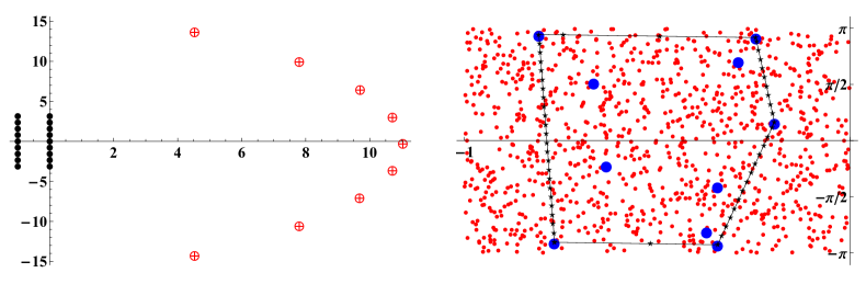
Figure 1. Left: the poles $\lambda_{k}$, $k=1,\dots,9$; right: the spectra of $A$ and $\widehat{A}$

References

- [1] A. C. Antoulas, Approximation of large-scale dynamical systems, Advances in Design and Control, vol. 6, Society for Industrial and Applied Mathematics (SIAM), Philadelphia, PA, 2005. MR 2155615
- [2] C. Badea, M. Crouzeix, and B. Delyon, Convex domains and -spectral sets, Math. Z. 252 (2006), no. 2, 345–365. MR 2207801
- [3] Zh. Bai and J. Demmel, Using the matrix sign function to compute invariant subspaces, SIAM J. Matrix Anal. Appl. 19 (1998), no. 1, 205–225. MR 1609964
- [4] G. A. Baker Jr. and P. Graves-Morris, Padé approximants, second ed., Encyclopedia of Mathematics and its Applications, vol. 59, Cambridge University Press, Cambridge, 1996. MR 1383091
- [5] B. Beckermann and M. Crouzeix, Operators with numerical range in a conic domain, Arch. Math. (Basel) 88 (2007), no. 6, 547–559. MR 2325887
- [6] B. Beckermann and L. Reichel, Error estimates and evaluation of matrix functions via the Faber transform, SIAM J. Numer. Anal. 47 (2009), no. 5, 3849–3883. MR 2576523
- [7] K. Burrage, N. Hale, and D. Kay, An efficient implicit FEM scheme for fractional-in-space reaction-diffusion equations, SIAM J. Sci. Comput. 34 (2012), no. 4, A2145–A2172. MR 2970400
- [8] R. Byers, Ch. He, and V. Mehrmann, The matrix sign function method and the computation of invariant subspaces, SIAM J. Matrix Anal. Appl. 18 (1997), no. 3, 615–632.
- [9] J. R. Cardoso and A. Sadeghi, Computation of matrix gamma function, BIT 59 (2019), no. 2, 343–370. MR 3974043
- [10] M. Crouzeix, Numerical range and functional calculus in Hilbert space, J. Funct. Anal. 244 (2007), no. 2, 668–690. MR 2297040
- [11] G. Dahlquist, Stability and error bounds in the numerical integration of ordinary differential equations, Inaugural dissertation, University of Stockholm, Almqvist & Wiksells Boktryckeri AB, Uppsala, 1958. MR 0100966
- [12] C. de Boor, Divided differences, Surv. Approx. Theory 1 (2005), 46–69.
- [13] V. Druskin, L. Knizhnerman, and M. Zaslavsky, Solution of large scale evolutionary problems using rational Krylov subspaces with optimized shifts, SIAM J. Sci. Comput. 31 (2009), no. 5, 3760–3780. MR 2556561
- [14] A. O. Gel′fond, Calculus of finite differences, second ed., GIFML, Moscow, 1959, (in Russian); translated by Hindustan Publishing Corp., Delhi, in series International Monographs on Advanced Mathematics and Physics, 1971. MR 0342890
- [15] by same author, Calculus of finite differences, International Monographs on Advanced Mathematics and Physics, Hindustan Publishing Corp., Delhi, 1971, Translation of the third Russian edition. MR 0342890
- [16] V. Grimm and M. Hochbruck, Rational approximation to trigonometric operators, BIT 48 (2008), no. 2, 215–229. MR 2430617
- [17] E. J. Grimme, Krylov projection methods for model reduction, Ph.D. thesis, University of Illinois at Urbana-Champaign, Urbana, Illinois, 1997.
- [18] K. E. Gustafson and D. K. M. Rao, Numerical range: the field of values of linear operators and matrices, Universitext, Springer-Verlag, New York, 1997. MR 1417493
- [19] S. Güttel, Rational Krylov approximation of matrix functions: numerical methods and optimal pole selection, GAMM-Mitt. 36 (2013), no. 1, 8–31. MR 3095912
- [20] E. Hairer, S. P. Nørsett, and G. Wanner, Solving ordinary differential equations. I. Nonstiff problems, second ed., Springer Series in Computational Mathematics, vol. 8, Springer-Verlag, Berlin, 1993. MR 1227985
- [21] Ph. Hartman, Ordinary differential equations, S. M. Hartman, Baltimore, Md., 1973, Corrected reprint. MR 0344555
- [22] N. J. Higham, Functions of matrices: theory and computation, Society for Industrial and Applied Mathematics (SIAM), Philadelphia, PA, 2008. MR 2396439
- [23] E. Hille and R. S. Phillips, Functional analysis and semi-groups, American Mathematical Society Colloquium Publications, vol. 31, Amer. Math. Soc., Providence, RI, 1957. MR 0089373
- [24] E. Jarlebring and T. Damm, The Lambert function and the spectrum of some multidimensional time-delay systems, Automatica 43 (2007), no. 12, 2124–2128. MR 2571740
- [25] Ch. Jordan, Calculus of finite differences, third ed., Chelsea Publishing Co., New York, 1965. MR 0183987
- [26] C. S. Kenney and A. J. Laub, The matrix sign function, IEEE Trans. Automat. Control 40 (1995), no. 8, 1330–1348. MR 1343800
- [27] V. G. Kurbatov and I. V. Kurbatova, An estimate of approximation of a matrix-valued function by an interpolation polynomial, Eurasian Math. J. 11 (2020), no. 1, 86–94. MR 4157279
- [28] Herng-Jer Lee, Chia-Chi Chu, and Wu-Shiung Feng, An adaptive-order rational Arnoldi method for model-order reductions of linear time-invariant systems, Linear Algebra Appl. 415 (2006), no. 2-3, 235–261. MR 2227774
- [29] S. M. Lozinskiĭ, Error estimate for numerical integration of ordinary differential equations. I, Izv. Vysš. Učebn. Zaved. Matematika (1958), no. 5, 52–90, (in Russian). MR 0145662
- [30] R. Mathias, Approximation of matrix-valued functions, SIAM J. Matrix Anal. Appl. 14 (1993), no. 4, 1061–1063. MR 1238920
- [31] J. W. Polderman and J. C. Willems, Introduction to mathematical systems theory. A behavioral approach, Texts in Applied Mathematics, vol. 26, Springer-Verlag, New York, 1998. MR 1480665
- [32] Th. Schmelzer and L. N. Trefethen, Computing the gamma function using contour integrals and rational approximations, SIAM J. Numer. Anal. 45 (2007), no. 2, 558–571. MR 2300287
- [33] V. Simoncini and D. B. Szyld, Recent computational developments in Krylov subspace methods for linear systems, Numer. Linear Algebra Appl. 14 (2007), no. 1, 1–59. MR 2289520
- [34] H. A. van der Vorst, Iterative Krylov methods for large linear systems, Cambridge Monographs on Applied and Computational Mathematics, vol. 13, Cambridge University Press, Cambridge, 2003. MR 1990752
- [35] V. V. Voevodin and Yu. A. Kuznetsov, Matritsy i vychisleniya [Matrices and computations], “Nauka”, Moscow, 1984, (in Russian). MR 758446
- [36] J. L. Walsh, Interpolation and approximation by rational functions in the complex domain, third ed., American Mathematical Society Colloquium Publications, vol. XX, American Mathematical Society, Providence, R.I., 1960. MR 0218587
- [37] S. Wolfram, The Mathematica book, fifth ed., Wolfram Media, New York, 2003.
- [38] K. Zhou, J. C. Doyle, and K. Glover, Robust and optimal control, vol. 40, Prentice-Hall, New Jersey, 1996.