Generic Neural Architecture Search via Regression

Abstract

Most existing neural architecture search (NAS) algorithms are dedicated to and evaluated by the downstream tasks, e.g., image classification in computer vision. However, extensive experiments have shown that, prominent neural architectures, such as ResNet in computer vision and LSTM in natural language processing, are generally good at extracting patterns from the input data and perform well on different downstream tasks. In this paper, we attempt to answer two fundamental questions related to NAS. (1) Is it necessary to use the performance of specific downstream tasks to evaluate and search for good neural architectures? (2) Can we perform NAS effectively and efficiently while being agnostic to the downstream tasks? To answer these questions, we propose a novel and generic NAS framework, termed Generic NAS (GenNAS). GenNAS does not use task-specific labels but instead adopts regression on a set of manually designed synthetic signal bases for architecture evaluation. Such a self-supervised regression task can effectively evaluate the intrinsic power of an architecture to capture and transform the input signal patterns, and allow more sufficient usage of training samples. Extensive experiments across 13 CNN search spaces and one NLP space demonstrate the remarkable efficiency of GenNAS using regression, in terms of both evaluating the neural architectures (quantified by the ranking correlation Spearman’s $\rho$ between the approximated performances and the downstream task performances) and the convergence speed for training (within a few seconds). For example, on NAS-Bench-101, GenNAS achieves 0.85 $\rho$ while the existing efficient methods only achieve 0.38. We then propose an automatic task search to optimize the combination of synthetic signals using limited downstream-task-specific labels, further improving the performance of GenNAS. We also thoroughly evaluate GenNAS’s generality and end-to-end NAS performance on all search spaces, which outperforms almost all existing works with significant speedup. For example, on NASBench-201, GenNAS can find near-optimal architectures within 0.3 GPU hour. Our code has been made available at: https://github.com/leeyeehoo/GenNAS

1 Introduction

Most existing neural architecture search (NAS) approaches aim to find top-performing architectures on a specific downstream task, such as image classification real2019regularized ; zoph2016neural ; liu2018darts ; cai2018proxylessnas ; su2021vision , semantic segmentation liu2019auto ; nekrasov2019fast ; shaw2019squeezenas , neural machine translation li2021bossnas ; wang2020hat ; so2019evolved or more complex tasks like hardware-software co-design hao2018deep ; hao2019fpga ; zhang2019skynet ; lin2020mcunet ; lin2021mcunetv2 . They either directly search on the target task using the target dataset (e.g., classification on CIFAR-10 zoph2016neural ; real2017large ), or search on a proxy dataset and then transfer to the target one (e.g. CIFAR-10 to ImageNet) zoph2018learning ; liu2018darts . However, extensive experiments show that prominent neural architectures are generally good at extracting patterns from the input data and perform well to different downstream tasks. For example, ResNet he2016deep being a prevailing architecture in computer vision, shows outstanding performance across various datasets and tasks chen2018encoder ; marsden2017resnetcrowd ; raghu2019transfusion , because of its advantageous architecture, the residual blocks. This observation motivates us to ask the first question: Is there a generic way to search for and evaluate neural architectures without using the specific knowledge of downstream tasks?

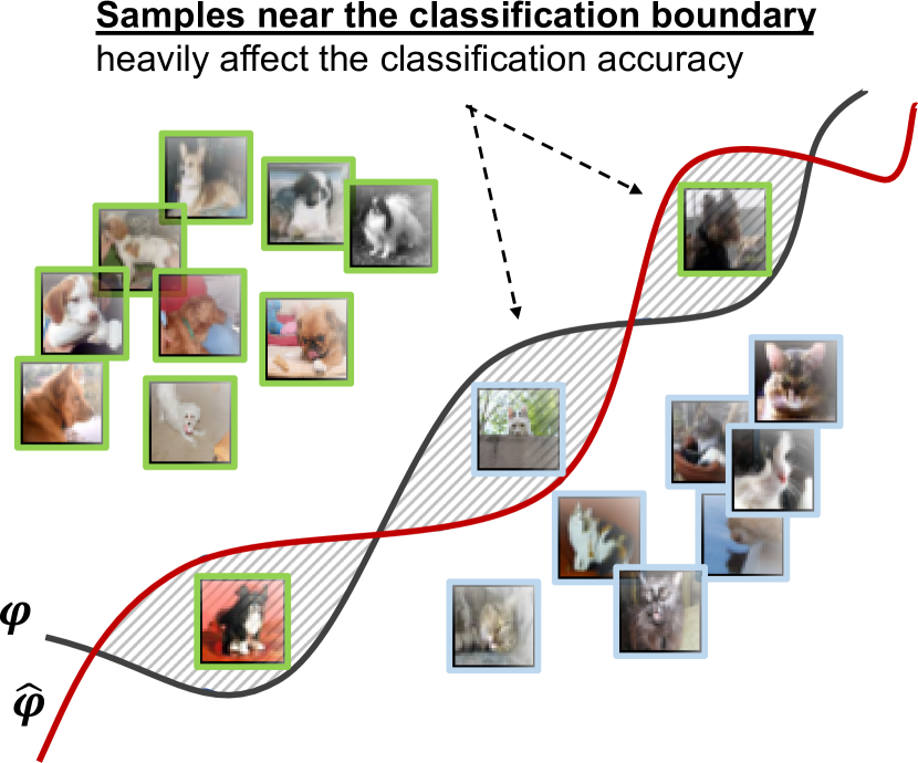
(a) Classification

(b) Regression

Figure 1: For classification, only samples near the decision boundary determine the classification accuracy. For regression, all samples equally contribute to the regression accuracy. Therefore, regression is better at leveraging all training samples than classification to achieve faster convergence.

Meanwhile, we observe that most existing NAS approaches directly use the final classification performance as the metric for architecture evaluation and search, which has several major issues. First, the classification accuracy is dominated by the samples along the classification boundary, while other samples have clearer classification outcomes compared to the boundary ones (as illustrated in Fig. 1(a)). Such phenomena can be observed in the limited number of effective support vectors in SVM hearst1998support , which also applies to neural networks because of the theory of neural tangent kernel jacot2018neural . Therefore, discriminating performance of classifiers needs many more samples than necessary (the indeed effective ones), causing a big waste. Second, a classifier tends to discard a lot of valuable information, such as finer-grained features and spatial information, by transforming input representations into categorical labels. This observation motivates us to ask the second question: Is there a more effective way that can make more sufficient use of input samples and better capture valuable information?

To answer the two fundamental questions for NAS, in this work, we propose a Generic Neural Architecture Search method, termed GenNAS. GenNAS adopts a regression-based proxy task using downstream-task-agnostic synthetic signals for network training and evaluation. It can efficiently (with near-zero training cost) and accurately approximate the neural architecture performance.

Insights. First, as opposed to classification, regression can efficiently make fully use of all the input samples, which equally contribute to the regression accuracy (Fig. 1b). Second, regression on properly-designed synthetic signals is essentially evaluating the intrinsic representation power of neural architectures, which is to capture and distinguish fundamental data patterns that are agnostic to downstream tasks. Third, such representation power is heavily reflected in the intermediate data of a network (as we will show in the experiments), which are regrettably discarded by classification.

Approach. First, we propose a regression proxy task as the supervising task to train, evaluate, and search for neural architectures (Fig. 2). Then, the searched architectures will be used for the target downstream tasks. To the best of our knowledge, we are the first to propose self-supervised regression proxy task instead of classification for NAS. Second, we propose to use unlabeled synthetic data (e.g., sine and random signals) as the groundtruth (Fig. 3) to measure neural architectures’ intrinsic capability of capturing fundamental data patterns. Third, to further boost NAS performance, we propose a weakly-supervised automatic proxy task search with only a handful of groundtruth architecture performance (e.g. 20 architectures), to determine the best proxy task, i.e., the combination of synthetic signal bases, targeting a specific downstream task, search space, and/or dataset (Fig. 4).

GenNAS Evaluation. The efficiency and effectiveness of NAS are dominated by neural architecture evaluation, which directs the search algorithm towards top-performing network architectures. To quantify how accurate the evaluation is, one widely used indicator is the network performance Ranking Correlation daniel1990applied between the prediction and groundtruth ranking, defined as Spearman’s Rho ($\rho$) or Kendall’s Tau ($\tau$). The ideal ranking correlation is 1 when the approximated and groundtruth rankings are exactly the same; achieving large $\rho$ or $\tau$ can significantly improve NAS quality zhou2020econas ; chu2019fairnas ; li2020random . Therefore, in the experiments (Sec. 4), we evaluate GenNAS using the ranking correlation factors it achieves, and then show its end-to-end NAS performance in finding the best architectures. Extensive experiments are done on 13 CNN search spaces and one NLP space klyuchnikov2020bench . Trained by the regression proxy task using only a single batch of unlabeled data within a few seconds, GenNAS significantly outperforms all existing NAS approaches on almost all the search spaces and datasets. For example, GenNAS achieves 0.87 $\rho$ on NASBench-101 ying2019bench , while Zero-Cost NAS abdelfattah2021zero , an efficient proxy NAS approach, only achieves 0.38. On end-to-end NAS, GenNAS generally outperforms others with large speedup. This implies that the insights behind GenNAS are plausible and that our proposed regression-based task-agnostic approach is generalizable across tasks, search spaces, and datasets.

Contributions. We summarize our contributions as follows:

• To the best of our knowledge, GenNAS is the first NAS approach using regression as the self-supervised proxy task instead of classification for neural architecture evaluation and search. It is agnostic to the specific downstream tasks and can significantly improve training and evaluation efficiency by fully utilizing only a handful of unlabeled data.

• GenNAS uses synthetic signal bases as the groundtruth to measure the intrinsic capability of networks that captures fundamental signal patterns. Using such unlabeled synthetic data in regression, GenNAS can find the generic task-agnostic top-performing networks and can apply to any new search spaces with zero effort.

• An automated proxy task search to further improve GenNAS performance.

• Thorough experiments show that GenNAS outperforms existing NAS approaches by large margins in terms of ranking correlation with near-zero training cost, across 13 CNN and one NLP space without proxy task search. GenNAS also achieves state-of-the-art performance for end-to-end NAS with orders of magnitude of speedup over conventional methods.

• With proxy task search being optional, GenNAS is fine-tuning-free, highly efficient, and can be easily implemented on a single customer-level GPU.

2 Related Work

NAS Evaluation. Network architecture evaluation is critical in guiding the search algorithms of NAS by identifying the top-performing architectures, which is also a challenging task with intensive research interests. Early NAS works evaluated the networks by training from scratch with tremendous computation and time cost zoph2018learning ; real2019regularized . To expedite, weight-sharing among the subnets sampled from a supernet is widely adopted liu2018darts ; li2020random ; cai2018proxylessnas ; xu2019pc ; li2020edd . However, due to the poor correlation between the weight-sharing and the final performance ranking, weight-sharing NAS can easily fail even in simple search spaces zela2019understanding ; dong2020bench . Yu et al. yu2019evaluating further pointed out that without accurate evaluation, NAS runs in a near-random fashion. Recently, zero-cost NAS methods mellor2020neural ; abdelfattah2021zero ; dey2021fear ; li2021flash have been proposed, which score the networks using their initial parameters with only one forward and backward propagation. Despite the significant speed up, they fail to identify top-performing architectures in large search spaces such as NASBench-101. To detach the time-consuming network evaluation from NAS, several benchmarks are developed with fully-trained neural networks within the NAS search spaces siems2020bench ; ying2019bench ; dong2020bench ; klyuchnikov2020bench ; su2021prioritized , so that researchers can assess the search algorithms alone in the playground.

NAS Transferability. To improve search efficiency, proxy tasks are widely used, on which the architectures are searched and then transferred to target datasets and tasks. For example, the CIFAR-10 classification dataset seems to be a good proxy for ImageNet zoph2018learning ; liu2018darts . Kornblith et al. kornblith2019better studied the transferability of 16 classification networks on 12 image classification datasets. NASBench-201 dong2020bench evaluated the ranking correlations across three popular datasets with 15625 architectures. Liu et al. liu2020labels studied the architecture transferability across supervised and unsupervised tasks. Nevertheless, training on a downsized proxy dataset is still inefficient (e.g. a few epochs of full-blown training liu2020labels ). In contrast, GenNAS significantly improves the efficiency by using a single batch of data while maintaining extremely good generalizability across different search spaces and datasets.

Self-supervised Learning. Self-supervised learning is a form of unsupervised learning, that the neural architectures are trained with automatically generated labels to gain a good degree of comprehension or understanding jing2020self ; dosovitskiy2014discriminative ; doersch2015unsupervised ; wang2015unsupervised ; liu2020labels . Liu et al. liu2020labels recently proposed three unlabeled classification proxy tasks, including rotation prediction, colorization, and solving jigsaw puzzles, for neural network evaluation. Though promising, this approach did not explain why such manually designed proxy tasks are beneficial and still used classification for training with the entire dataset. In contrast, GenNAS uses regression with only a single batch of synthetic data.

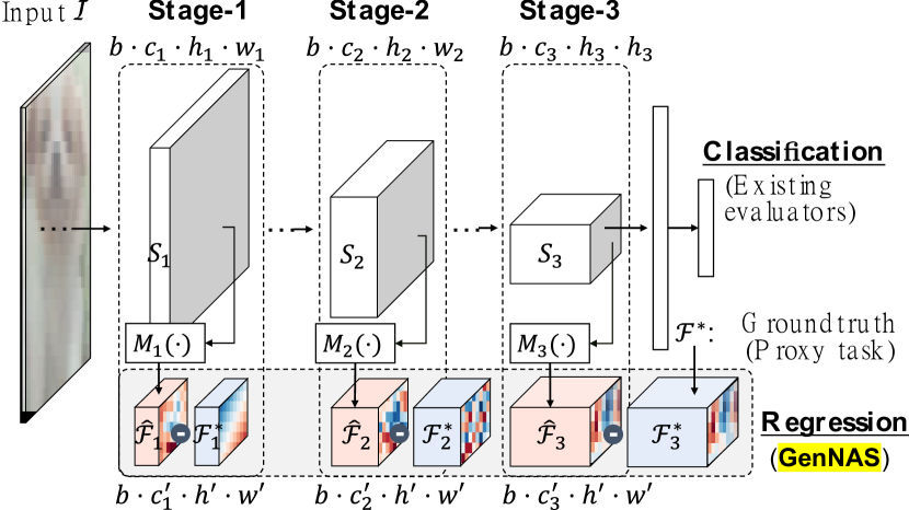
(a) CNN regression

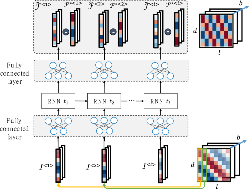
(b) RNN regression

Figure 2: Regression architectures on CNNs and RNNs. (a) On CNNs, we remove the final classifier and extract multiple stages of intermediate feature map for training. (b) On RNNs, we construct a many-to-many regression task, where the input and output tensors have the same size.

3 Proposed GenNAS

In Section 3.1, we introduce the main concepts of task-agnostic GenNAS: 1) the proposed regression proxy task for both CNN architectures and recurrent neural network (RNN) architectures; 2) the synthetic signal bases used for representing the fundamental data patterns as the proxy task. In Section 3.2, we introduce the automated proxy task search.

3.1 GenNAS

3.1.1 Regression Architectures

Training using unlabeled regression is the key that GenNAS being agnostic to downstream tasks. Based on the insights discussed in Section 1, the principle of designing the regression architecture is to fully utilize the abundant intermediate information rather than the final classifier.

Regression on CNNs. Empirical studies show that CNNs learn fine-grained high-frequency spatial details in the early layers and produce semantic features in the late layers wang2020high . Following this principle, as shown in Fig. 2a, we construct a Fully Convolutional Network (FCN) long2015fully by removing the final classifier of a CNN, and then extract the FCN’s intermediate feature maps from multiple stages. We denote the number of stages as $N$. Inputs. The inputs to the FCN are unlabeled real images, shaped as a tensor $\mathcal{I}\in\mathbb{R}^{b\times 3\times h\times w}$, where $b$ is the batch size, and $h$ and $w$ are the input image size. Outputs. From each stage $i$ ($1\leq i\leq N$) of the FCN, we first extract a feature map tensor, denoted by $\mathcal{F}_{i}\in\mathbb{R}^{b\times c_{i}\times h_{i}\times w_{i}}$, and reshape it as $\hat{\mathcal{F}}_{i}\in\mathbb{R}^{b\times c_{i}^{\prime}\times h^{\prime}\times w^{\prime}}$ through a convolutional layer $M_{i}$ by $\hat{\mathcal{F}}_{i}=M_{i}({\mathcal{F}}_{i})$ (with downsampling if $w_{i}>w^{\prime}$ or $h_{i}>h^{\prime}$). The outputs are the tensors $\hat{\mathcal{F}}_{i}$, which encapsulate the captured signal patterns from different stages. Groundtruth. We construct a synthetic signal tensor for each stage as the groundtruth, which serves as part of the proxy task. A synthetic tensor is a combination of multiple synthetic signal bases (more details in Section 3.1.2), denoted by $\mathcal{F}_{i}^{*}$. We compare $\hat{\mathcal{F}}_{i}$ with $\mathcal{F}_{i}^{*}$ for training and evaluating the neural architectures. During training, we use MSE loss defined as $\mathcal{L}=\sum^{N}_{i=1}\textbf{E}[(\mathcal{F}^{*}_{i}-\hat{\mathcal{F}}_{i})^{2}]$; during validation, we adjust each stage’s output importance as $\mathcal{L}=\sum^{N}_{i=1}\frac{1}{2^{N-i}}\textbf{E}[(\mathcal{F}^{*}_{i}-\hat{\mathcal{F}}_{i})^{2}]$ since the feature map tensors of later stages are more related to the downstream task’s performance. The detailed configurations of $N$, $h^{\prime}$, $w^{\prime}$, and $c_{i}^{\prime}$ are provided in the experiments.

Regression on RNNs. The proposed regression proxy task can be similarly applied to NLP tasks using RNNs. Most existing NLP models use a sequence of word-classifiers as the final outputs, whose evaluations are thus based on the word classification accuracy hochreiter1997long ; mikolov2010recurrent ; vaswani2017attention . Following the same principle for CNNs, we design a many-to-many regression task for RNNs as shown in Fig. 2b. Instead of using the final word-classifier’s output, we extract the output tensor of the intermediate layer before it. Inputs. For a general RNN model, the input is a random tensor $\mathcal{I}\in\mathbb{R}^{l\times b\times d}$, where $l$ is the sequence length, $b$ is the batch size, and $d$ is the length of input/output word vectors. Given a sequence of length $l$, the input to the RNN each time is one slice of the tensor $\mathcal{I}$, denoted by $\mathcal{I}^{(i)}\in\mathbb{R}^{b\times d}$, $1\leq i\leq l$. Outputs. The output is $\hat{\mathcal{F}}\in\mathbb{R}^{l\times b\times d}$, where a slice of $\hat{\mathcal{F}}$ is $\hat{\mathcal{F}}^{(i)}\in\mathbb{R}^{b\times d}$. Groundtruth. Similar to the CNN case, we generate a synthetic signal tensor ${\mathcal{F}^{*}}$ as the proxy task groundtruth.

3.1.2 Synthetic Signal Bases

The proxy task for regression aims to capture the task-agnostic intrinsic learning capability of the neural architectures, i.e., representing various fundamental data patterns. For example, good CNNs must be able to learn different frequency signals to capture image features xu2019frequency . Here, we design four types of synthetic signal basis: (1) 1-D frequency basis (Sin1D); (2) 2-D frequency basis (Sin2D); (3) Spatial basis (Dot and GDot); (4) Resized input signal (Resize). Sin1D and Sin2D represent frequency information, Dot and GDot represent spatial information, and Resize reflects the CNN’s scale-invariant capability. The combinations of these signal bases, especially with different sine frequencies, can represent a wide range of complicated real-world signals tolstov2012fourier . If a network architecture is good at learning such signal basis and their simple combinations, it is more likely to be able to capture real-world signals from different downstream tasks.

Fig.3(a) depicts examples of synthetic signal bases, where each base is a 2D signal feature map. Sin1D is generated by $\sin(2{\pi}fx+\phi)$ or $\sin(2{\pi}fy+\phi)$, and Sin2D is generated by $\sin(2{\pi}f_{x}x+2{\pi}f_{y}y+\phi)$, where $x$ and $y$ are pixel indices. Dot is generated according to biased Rademacher distribution montgomery1990distribution by randomly setting $k\%$ pixels to $\pm 1$ on zeroed feature maps. GDot is generated by applying a Gaussian filter with $\sigma=1$ on Dot and normalizing between $\pm 1$. The synthetic signal tensor $\mathcal{F}^{*}$ (the proxy task groundtruth) is constructed by stacking the 2D signal feature maps along the channel dimension (CNNs) or the batch dimension (for RNNs). Fig.3b shows examples of stacked synthetic tensor $\mathcal{F}^{*}$ for CNN architectures. Within one batch of input images, we consider two settings: global and local. The global setting means that the synthetic tensor is the same for all the inputs within the batch, as the Sin2D Global in Fig. 3(b), aiming to test the network’s ability to capture invariant features from different inputs; the local setting uses different synthetic signal tensors for different inputs, as the Dot Local in Fig.3(b), aiming to test the network’s ability to distinguish between images. For CNNs, the real images are only used by resize, and both global and local settings are used. For RNNs, we only use synthetic signals and the local setting, because resizing natural language or time series, the typical input of RNNs, does not make as much sense as resizing images for CNNs.

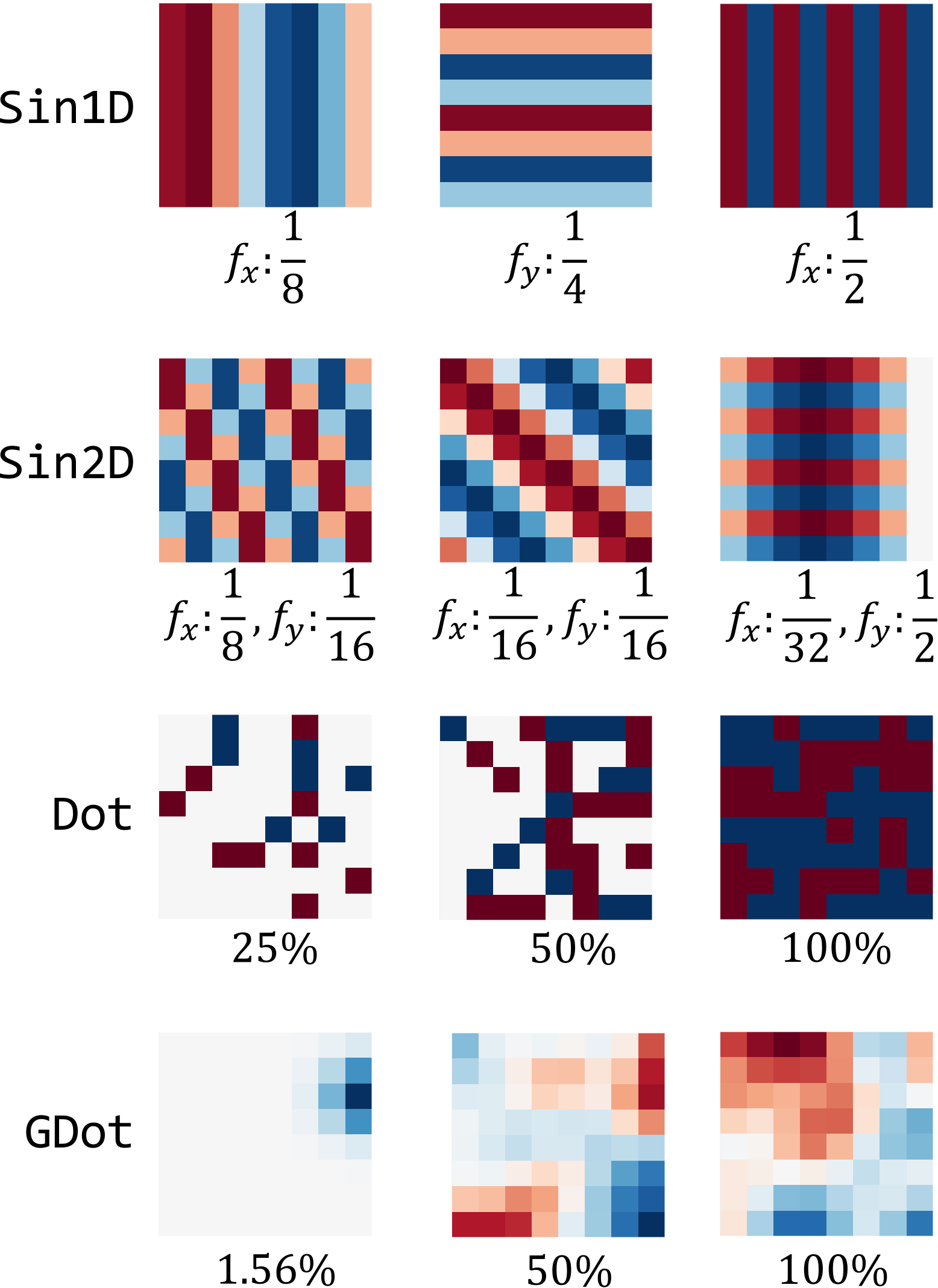
(a) Examples of signal bases

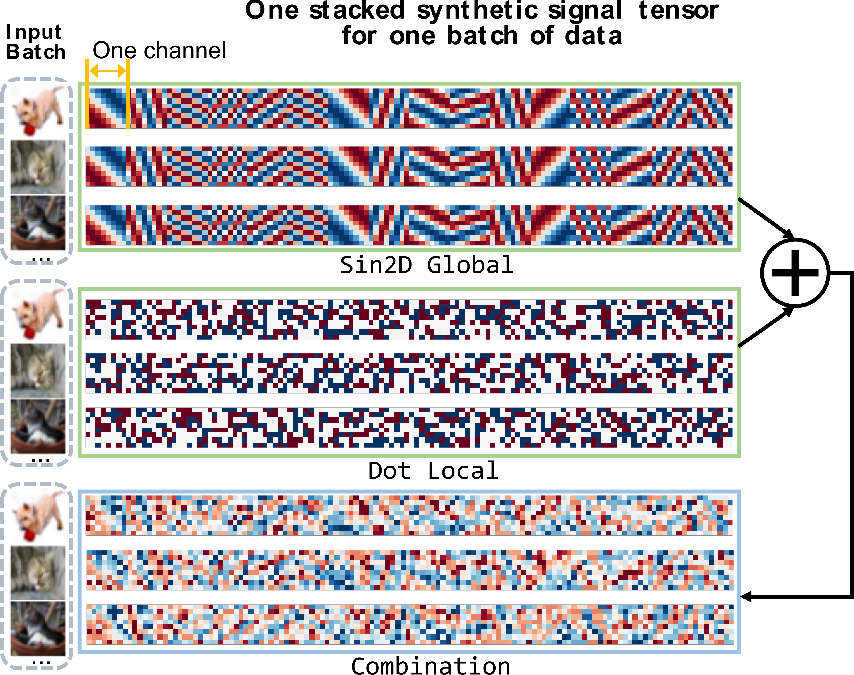
(b) Examples of synthetic signal tensors

Figure 3: (a) Examples of synthetic signal bases (2D feature maps). (b) Examples of the synthetic signal tensors by stacking 2D feature maps along the channel dimension for CNN architectures.

3.2 Proxy Task Search

While the synthetic signals can express generic features, the importance of these features for different tasks, NAS search spaces, and datasets may be different. Therefore, we further propose a weakly-supervised proxy task search, to automatically find the best synthetic signal tensor, i.e., the best combination of synthetic signal bases. We define the proxy task search space as the parameters when generating the synthetic signal tensors. As illustrated in Fig. 4, first, we randomly sample a small subset (e.g., 20) of the neural architectures in the NAS search space and obtain their groundtruth ranking on the target task (e.g., image classification). We then train these networks using different proxy tasks and calculate the performance ranking correlation $\rho$ of the proxy and the target task. We use the regularized tournament selection evolutionary algorithm real2019regularized to search for the task that results in the largest $\rho$, where $\rho$ is the fitness function.

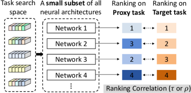
Figure 4: Proxy task search.

Proxy Task Search Space. We consider the following parameters as the proxy task search space. (1) Noise. We add noise to the input data following the distribution of parameterized Gaussian or uniform distribution. (2) The number of channels for each synthetic signal tensor ($c_{i}$ in $\mathcal{F}_{i}^{*}\in\mathbb{R}^{b\times c_{i}\times h^{\prime}\times w^{\prime}}$) can be adjusted. (3) Signal parameters, such as the frequency $f$ and phase $\phi$ in Sin, can be adjusted. (4) Feature combination. Each synthetic signal tensor uses either local or global, and tensors can be selected and summed up. Detailed parameters can be found in the supplemental material.

4 Experiments 

We perform the following evaluations for GenNAS. First, to show the true power of regression, we use manually designed proxy tasks without task search and apply the same proxy task on all datasets and search spaces. We demonstrate that the GenNAS generally excels in all different cases with zero task-specific cost, thanks to unlabeled self-supervised regression proxy task. Specifically, in Section 4.1, we analyze the effectiveness of the synthetic signal bases and manually construct two sets of synthetic tensors as the baseline proxy tasks; in Section 4.2, we extensively evaluate the proposed regression approach in 13 CNN search spaces and one NLP search space. Second, in Section 4.3, we evaluate the proxy task search and demonstrate the remarkable generalizability by applying one searched task to all NAS search spaces with no change. Third, in Section 4.4, we evaluate GenNAS on end-to-end NAS tasks, which outperforms existing works with significant speedup.

Experiment Setup. We consider 13 CNN NAS search spaces including NASBench-101 ying2019bench , NASBench-201 dong2020bench , Network Design Spaces (NDS) radosavovic2019network , and one NLP search space, NASBench-NLP klyuchnikov2020bench . All the training is conducted using only one batch of data with batch size 16 for 100 iterations. Details of NAS search spaces and experiment settings are in the supplemental material.

4.1 Effectiveness of Synthetic Signals

The synthetic signal analysis is performed on NASBench-101 using CIFAR-10 dataset. From the whole NAS search space, 500 network architectures are randomly sampled with a known performance ranking provided by NASBench-101. We train the 500 networks using different synthetic signal tensors and calculate their ranking correlations with respect to the groundtruth ranking. Using the CNN architecture discussed in Section 3.1.1, we consider three stages, $S_{1}$ to $S_{3}$ for $N=3$; the number of channels is 64 for each stage. For Sin1D and Sin2D, we set three ranges for frequency $f$: low (L) $f\in(0,0.125)$ , medium (M) $f\in(0.125,0.375)$, and high (H) $f\in(0.375,0.5)$. Within each frequency range, 10 signals are generated using uniformly sampled frequencies. For Dot and GDot, we randomly set $50\%$ and $100\%$ pixels to $\pm 1$ on the zeroized feature maps.

Table 1: Ranking correlation (Spearman’s $\rho$) analysis of different synthetic signals on NASBench-101.

Stage	Sin1D			Sin2D			Dot		GDot		Resize	Zero
	L	M	H	L	M	H	50%	100%	50%	100%
$S_{1}$	0.13	0.43	0.64	0.14	0.53	0.63	0.55	0.62	0.18	0.16	0.56	0.17
$S_{2}$	0.03	0.52	0.79	0.05	0.73	0.72	0.64	0.69	0.03	0.02	0.73	0.18
$S_{3}$	0.08	0.77	0.80	0.23	0.78	0.72	0.76	0.81	0.16	0.17	0.80	0.22
GenNAS-combo:: 0.85

The results of ranking correlations are shown in Table 1. The three stages are evaluated independently and then used together. Among the three stages, Sin1D and Sin2D within medium and high frequency work better in $S_{1}$ and $S_{2}$, while the high frequency Dot and resize work better in $S_{3}$. The low frequency signals, such as GDot, Sin1D-L, Sin2D-L, and the extreme case zero tensors, result in low ranking correlations; we attribute to their poor distinguishing ability. We also observe that the best task in $S_{3}$ (0.81) achieves higher $\rho$ than $S_{1}$ (0.64) and $S_{2}$ (0.79), which is consistent with the intuition that the features learned in deeper stages have more impact to the final network performance.

When all three stages are used, where each stage uses its top-3 signal bases, the ranking correlation can achieve 0.85, higher than the individual stages. This supports our assumption in Section 3.1.1 that utilizing more intermediate information of a network is beneficial. From this analysis, we choose two top-performing proxy tasks in the following evaluations to demonstrate the effectiveness of regression: GenNAS-single – the best proxy task with a single signal tensor Dot%100 used only in $S_{3}$, and GenNAS-combo – the combination of the three top-performing tasks in three stages.

4.2 Effectiveness and Efficiency of Regression without Proxy Task Search

To quantify how well the proposed regression can approximate the neural architecture performance with only one batch of data within seconds, we use the ranking correlation, Spearman’s $\rho$, as the metric abdelfattah2021zero ; liu2020labels ; zela2019understanding . We use the two manually designed proxy tasks (GenNAS-single and GenNAS-combo) without proxy task search to demonstrate that GenNAS is generic and can be directly applied to any new search spaces with zero task-specific search efforts. The evaluation is extensively conducted on 13 CNN search spaces and 1 NLP search space, and the results are summarized in Table 2.

Table 2: GenNAS ranking correlation evaluation using the correlation Spearman’s $\rho$. GenNAS-single and GenNAS-combo use a single or a combination of synthetic signals that are manually designed without proxy task search. GenNAS search-N, -D, -R mean the proxy task is searched on NASBench-101, NDS DARTS design space, and NDS ResNet design space, respectively. The top-1/2/3 results of GenNAS and efficient NAS baselines are highlighted by ^†/^‡/^§ respectively for each task. The values with superscripts are obtained after task search (^s) or transferred (^t) from a previous searched task. Methods like jig@ep10 which is 40x slower compared to the GenNAS in prediction are not considered as efficient ones.

NASBench-101
Dataset	NASWOT	synflow	jig@ep10	rot@ep10	col@ep10	cls@ep10	GenNAS
	mellor2020neural	abdelfattah2021zero	$>40\times$ slower				single	combo	search-N
CIFAR-10	0.34	0.38	0.69	0.85	0.71	0.81	$0.81^{\mathsection}$	$0.85^{\ddagger}$	0.87†s
ImgNet	0.21	0.09	0.72	0.82	0.67	0.79	$0.65^{\mathsection}$	$\textbf{0.73}^{\dagger}$	$0.71^{\ddagger t}$

NASBench-201
Dataset	NASWOT	synflow	jacob_cov	snip	cls@ep10	vote	EcoNAS	GenNAS
					$>40\times$ slower		$>60\times$ slower	single	combo	search-N
CIFAR-10	$0.79^{\mathsection}$	0.72	0.76	0.57	0.75	0.81	0.81	0.77	$0.87^{\ddagger}$	$\textbf{0.90}^{\dagger t}$
CIFAR-100	0.81	0.76	0.70	0.61	0.75	$0.83^{\ddagger}$	0.75	0.69	$0.82^{\mathsection}$	$\textbf{0.84}^{\dagger t}$
ImgNet16	$0.78$	0.73	0.73	0.59	0.68	0.81§	0.77	0.70	$0.81^{\ddagger}$	$\textbf{0.87}^{\dagger t}$

Neural Design Spaces
Dataset	NAS-Space	NASWOT	synflow	cls@ep10	GenNAS
				$>40\times$ slower	single	combo	search-N	search-D	search-R
CIFAR-10	DARTS	0.65	0.41	0.63	0.43	0.68	0.71§t	0.86†s	0.82‡t
	DARTS-f	0.31	0.09	0.82	0.51	0.59†	0.53§t	0.58‡t	0.52t
	Amoeba	0.33	0.06	0.67	0.52	0.64	0.68§t	0.78†t	0.72‡t
	ENAS	0.55	0.19	0.66	0.56	0.70§	0.67t	0.82†t	0.78‡t
	ENAS-f	0.43	0.26	0.86	0.65	0.65	0.67§t	0.73†t	0.67‡t
	NASNet	0.40	0.00	0.64	0.56	0.66§	0.65t	0.77†t	0.71‡t
	PNAS	0.51	0.26	0.50	0.32	0.58	0.59§t	0.76†t	0.71‡t
	PNAS-f	0.10	0.32	0.85	0.45	0.48§	0.56†t	0.55‡t	0.47t
	ResNet	0.26	0.22	0.65	0.34	0.52	0.55§t	0.54‡t	0.83†s
	ResNeXt-A	0.65§	0.48	0.86	0.57	0.61	0.80‡t	0.63t	0.84†t
	ResNeXt-B	0.60§	0.60‡	0.66	0.26	0.30	0.53t	0.55t	0.71†t
ImageNet	DARTS	0.66	0.21	–	0.61	0.75‡	0.70§t	0.84†t	0.55t
	DARTS-f	0.20	0.37	–	0.68$\mathsection$	0.69‡	0.67t	0.69†t	0.59t
	Amoeba	0.42	0.25	–	0.63	0.72§	0.73‡t	0.80†t	0.67t
	ENAS	0.69§	0.17	–	0.59	0.70‡	0.58t	0.81†t	0.65t
	NASNet	0.51	0.01	–	0.52	0.59§	0.52t	0.70†t	0.61‡t
	PNAS	0.60‡	0.14	–	0.28	0.39	0.45§t	0.62†t	0.40t
	ResNeXt-A	0.72	0.42	–	0.80§	0.84‡	0.75t	0.62t	0.87†t
	ResNeXt-B	0.63	0.31	–	0.71‡	0.79†	0.51t	0.60t	0.64§t

NASBench-NLP
Dataset	grad_norm	snip	grasp	synflow	jacob_cov	ppl@ep3	GenNAS
						$>192\times$ slower	single	combo	search
PTB	0.21	0.19	0.16	0.34	0.56§	0.79	0.73	0.74‡	0.81†s

On NASBench-101, GenNAS is compared with zero-cost NAS abdelfattah2021zero ; mellor2020neural and the latest classification based approaches liu2020labels . Specifically, NASWOT mellor2020neural is a zero-training approach that predicts a network’s trained accuracy from its initial state by examining the overlap of activations between datapoints. Abdelfattah et al. abdelfattah2021zero proposed proxies such as synflow to evaluate the networks, where the synflow computes the summation of all the weights multiplied by their gradients and has the best reported performance in the paper. Liu et al. liu2020labels used three unsupervised classification training proxies, namely rotation prediction (rot), colorization (col), and solving jigsaw puzzles (jig), and one supervised classification proxy (cls).

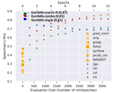
Figure 5: The effectiveness of regression-based proxy task. GenNAS significantly outperforms all the existing NAS evaluation approaches regarding ranking correlation, with near-zero training cost.

We report their results after 10 epochs (@ep10) for each proxy. The results show that GenNAS-single and GenNAS-combo achieve 0.81 and 0.85 $\rho$ on CIFAR-10, and achive 0.73 on ImageNet, respectively, much higher than NASWOT and synflow. It is also comparable and even higher comparing with the classification proxies, cls@ep5 and cls@ep10. Notably, the classification proxies need to train for 10 epochs using all training data, while GenNAS requires only a few seconds, more than 40$\times$ faster. On NASBench-201, we further compare with vote abdelfattah2021zero and EcoNAS zhou2020econas . EcoNAS is a recently proposed reduced-training proxy NAS approach. Vote abdelfattah2021zero adopts the majority vote between three zero-training proxies including synflow, jacob_cov, and snip. Clearly, GenNAS-combo outperforms all these methods regarding ranking correlation, and is also $60\times$ faster than EcoNAS and $40\times$ faster than cls@ep10. On Neural Design Spaces, we evaluate GenNAS on both CIFAR-10 and ImageNet datasets. Comparing with NASWOT and synflow, GenNAS-single and GenNAS-combo achieve higher $\rho$ in almost all cases. Also, synflow performs poorly on most of the NDS search spaces especially on ImageNet dataset, while GenNAS achieves even higher $\rho$. Extending to NLP search space, NASBench-NLP, GenNAS-single and GenNAS-combo achieve 0.73 and 0.74 $\rho$, respectively, surpassing the best zero-proxy method (0.56). Comparing with the ppl@ep3, the architectures trained on PTB marcus1993building dataset after three epochs, GenNAS is $192\times$ faster in prediction.

Fig. 5 visualizes the comparisons between GenNAS and existing NAS approaches on NASBench-101, CIFAR-10. Clearly, regression-based GenNAS (single, combo) significantly outperforms the existing NAS with near-zero training cost, showing remarkable effectiveness and high efficiency.

4.3 Effectiveness of Proxy Task Search and Transferability

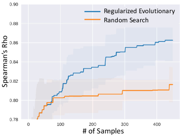
Figure 6: Proxy task search.

Effectiveness of Proxy Task Search. While the unsearched proxy tasks can already significantly outperform all existing approaches (shown in Section 4.2), we demonstrate that the proxy task search described in Section 3.2 can further improve the ranking correlation. We adopt the regularized evolutionary algorithm real2019regularized . The population size is $50$; the tournament sample size is $10$; the search runs $400$ iterations. We randomly select 20 architectures with groundtruth for calculating the $\rho$. More settings can be found in the supplemental material. Fig. 6 shows the search results averaged from 10 runs with different seeds. It shows that the regularized evolutionary algorithm is more effective comparing with random search, where the correlations of 20 architectures are $0.86\pm 0.02$ and $0.82\pm 0.01$, respectively.

In the following experiments, we evaluate three searched proxy tasks, denoted by GenNAS search-N, -D, and -R, meaning that the task is searched on NASBench-101, NDS DARTS search space, and NDS ResNet search space, respectively. We study the performance and transferability of the searched tasks on all NAS search spaces. Proxy task search is done on a single GPU GTX 1080Ti. On NASBench-101 (GenNAS-N), ResNeXt (GenNAS-R), and DARTS (GenNAS-D), the search time is 5.75, 4, and 12.25 GPU hours, respectively. Once the proxy tasks is searched, it can be used to evaluate any architectures in the target search space and can be transferred to other search spaces.

GenNAS with Searched/Transferred Proxy Task. The performance of GenNAS-search-N, -D, and -R proxy tasks is shown in Table 2. First, in most cases, proxy task search improves the ranking correlation. For example, in NDS, using the proxy task searched on DARTS space (search-D) outperforms other GenNAS settings on DARTS-like spaces, while using proxy task search-R on ResNet-like spaces outperforms others as well. In NASBench-NLP, the proxy task search can push the ranking correlation to 0.81, surpassing the ppl@ep3 (0.79). Such results demonstrate the effectiveness of our proposed proxy task search. Second, the searched proxy task shows great transferability: the proxy task searched on NASBench-101 (search-N) generally works well for other search spaces, i.e., NASBench-201, NDS, and NASBench-NLP. This further emphasizes that the fundamental principles for top-performing neural architectures are similar across different tasks and datasets. Fig. 5 visualizes the performance of GenNAS comparing with others.

Table 3: GenNAS end-to-end NAS results comparing with the state-of-the-art NAS approaches, showing test accuracy (%) on different NAS-spaces and datasets. ^⋆ denotes a method that is replicated with the same regularized evolutionary algorithm in Section 4.4 for fair comparison. On NASBench-201, the GPU hours do not include task search since GenNAS-N is transferred from NASBench-101. The values with superscripts are obtained after task search (^s) or transferred (^t) from a previous searched task.

NASBench-101(CIFAR-10)
Optimal	NASWOT⋆	synflow⋆	Halfway⋆	GenNAS-N
94.32	93.30$\pm$0.002	91.31$\pm$0.02	93.28$\pm$0.002	93.92$\pm$0.004s
NASBench-201
Dataset	Optimal	RSPS	DARTS-V2	GDAS	SETN	ENAS	NASWOT	GenNAS-N
CIFAR-10	94.37	84.07$\pm$3.61	54.30$\pm$0.00	93.61$\pm$0.09	87.64$\pm$0.00	53.89$\pm$0.58	92.96$\pm$0.80	94.18$\pm$0.10t
CIFAR-100	73.49	58.33$\pm$4.34	15.61$\pm$0.00	70.61$\pm$0.26	56.87$\pm$7.77	15.61$\pm$0.00	70.03$\pm$1.16	72.56$\pm$0.74t
ImgNet16	47.31	26.28$\pm$3.09	16.32$\pm$0.00	41.71$\pm$0.98	32.52$\pm$0.21	14.84$\pm$2.10	44.43$\pm$2.07	45.59$\pm$0.54t
GPU hours		2.2	9.9	8.8	9.5	3.9	0.1	0.3
Neural Design Spaces (CIFAR-10)
NAS-Space	Optimal	NASWOT⋆	synflow⋆	cls@ep10⋆	GenNAS-N	GenNAS-R	GenNAS-D
ResNet	95.30	92.81$\pm$0.10	93.52$\pm$0.31	94.51$\pm$0.20	94.48$\pm$0.24t	94.63$\pm$0.23t	94.77$\pm$0.13s
ResNeXt-A	94.99	93.39$\pm$0.67	94.05$\pm$0.48	94.24$\pm$ 0.22	94.25$\pm$0.21t	94.12$\pm$0.20t	94.37$\pm$0.14t
ResNeXt-B	95.12	93.56$\pm$0.33	93.65$\pm$0.64	94.33$\pm$0.26	94.29$\pm$0.24t	94.26$\pm$0.35t	94.23$\pm$0.32t

4.4 GenNAS for End-to-End NAS

Finally, we evaluate GenNAS on the end-to-end NAS tasks, aiming to find the best neural architectures within the search space. Table 3 summarizes the comparisons with the state-of-the-art NAS approaches, including previously used NASWOT, synflow, cls@ep10, and additionally Halfway ying2019bench , RSPS li2020random , DARTS-V1 liu2018darts , DARTS-V2, GDAS dong2019searching , SETN dong2019one , and ENAS pham2018efficient . Halfway is the NASBench-101-released result using half of the total epochs for network training. In all the searches during NAS, we do not use any tricks such as warmup selection abdelfattah2021zero or groundtruth query to compensate the low rank correlations. We fairly use a simple yet effective regularized evolutionary algorithm real2019regularized and adopt the proposed regression loss as the fitness function. The population size is $50$ and the tournament sample size is $10$ with 400 iterations. On NASBench-101, GenNAS finds better architectures than NASWOT and Halfway while being up to 200$\times$ faster. On NASBench-201, GenNAS finds better architectures than the state-of-the-art GDAS within 0.3 GPU hours, being $30\times$ faster. Note that GenNAS uses the proxy task searched on NASBench-101 and transferred to NASBench-201, demonstrating remarkable transferability. On Neural Design Spaces, GenNAS finds better architectures than the cls@ep10 using labeled classification while being 40$\times$ faster. On NASBench-NLP, GenNAS finds architectures that achieve 0.246 (the lower the better) average final regret score $r$, outperforming the ppl@ep3 (0.268) with 192$\times$ speed up. The regret score $r$ at the moment $t$ is $r(t)=L(t)-L^{\star}$, where $L(t)$ is the testing log perplexity of the best found architecture according to the prediction by the moment, and $L^{\star}=4.36$ is the lowest testing log perplexity in the whole dataset achieved by LSTM hochreiter1997long architecture.

On DARTS search space, we also perform the end-to-end search on ImageNet-1k deng2009imagenet dataset. We fix the depth (layer) of the networks to be 14 and adjust the width (channel) so that the # of FLOPs is between 500M to 600M. We evaluate two strategies: one without task search using GenNAS-combo (see Table 1), and the other GenNAS-D14 with proxy task search on DARTS search space with depth 14 and initial channel 16. The training settings follow TENAS chen2021neural . The results are shown in Table 4. We achieve top-1/5 test error of 25.1/7.8 using GenNAS-combo and top-1/5 test error of 24.3/7.2 using GenNAS-D14, which are on par with existing NAS architectures. GenNAS-combo is much faster than existing works, while GenNAS-D14 pays extra search time cost. Our next step is to investigate the searched tasks and demonstrate the generalization and transferrability of those searched tasks to further reduce the extra search time cost.

Table 4: Comparisons with state-of-the-art NAS methods on ImageNet under the mobile setting. ^∗ is the time for proxy task search.

Method	Test Err. (%)		Params	FLOPS(M)	Search Cost	Searched	Searched
	top-1	top-5	(M)	(M)	(GPU days)	Method	dataset
NASNet-A zoph2018learning	26.0	8.4	5.3	564	2000	RL	CIFAR-10
AmoebaNet-C real2019regularized	24.3	7.6	6.4	570	3150	evolution	CIFAR-10
PNAS liu2018progressive	25.8	8.1	5.1	588	225	SMBO	CIFAR-10
DARTS(2nd order) liu2018darts	26.7	8.7	4.7	574	4.0	gradient-based	CIFAR-10
SNAS xie2018snas	27.3	9.2	4.3	522	1.5	gradient-based	CIFAR-10
GDAS dong2019searching	26.0	8.5	5.3	581	0.21	gradient-based	CIFAR-10
P-DARTS chen2019progressive	24.4	7.4	4.9	557	0.3	gradient-based	CIFAR-10
P-DARTS	24.7	7.5	5.1	577	0.3	gradient-based	CIFAR-100
PC-DARTS xu2019pc	25.1	7.8	5.3	586	0.1	gradient-based	CIFAR-10
TE-NAS chen2021neural	26.2	8.3	6.3	-	0.05	training-free	CIFAR-10
PC-DARTS	24.2	7.3	5.3	597	3.8	gradient-based	ImageNet
ProxylessNAS cai2018proxylessnas	24.9	7.5	7.1	465	8.3	gradient-based	ImageNet
UNNAS-jig liu2020labels	24.1	-	5.2	567	2	gradient-based	ImageNet
TE-NAS	24.5	7.5	5.4	599	0.17	training-free	ImageNet
GenNAS-combo	25.1	7.8	4.8	559	0.04	evolution+few-shot	CIFAR-10
GenNAS-D14	24.3	7.2	5.3	599	0.7∗+0.04	evolution+few-shot	CIFAR-10

These end-to-end NAS experiments strongly suggest that GenNAS is generically efficient and effective across different search spaces and datasets.

5 Conclusion

In this work, we proposed GenNAS, a self-supervised regression-based approach for neural architecture training, evaluation, and search. GenNAS successfully answered the two questions at the beginning. (1) GenNAS is a generic task-agnostic method, using synthetic signals to capture neural networks’ fundamental learning capability without specific downstream task knowledge. (2) GenNAS is an extremely effective and efficient method using regression, fully utilizing all the training samples and better capturing valued information. We show the true power of self-supervised regression via manually designed proxy tasks that do not need to search. With proxy search, GenNAS can deliver even better results. Extensive experiments confirmed that GenNAS is able to deliver state-of-the-art performance with near-zero search time, in terms of both ranking correlation and the end-to-end NAS tasks with great generalizability.

6 Acknowledgement

We thank IBM-Illinois Center for Cognitive Computing Systems Research (C3SR) for supporting this research. We thank all reviewers and the area chair for valuable discussions and feedback. This work utilizes resources kindratenko2020hal supported by the National Science Foundation’s Major Research Instrumentation program, grant #1725729, as well as the University of Illinois at Urbana-Champaign. P.L. is also partly supported by the 2021 JP Morgan Faculty Award and the National Science Foundation award HDR-2117997.

Appendix A Appendix

A.1 NAS Search Spaces

NASBench-101 introduces a large and expressive search space with 423k unique convolutional neural architectures and training statistics on CIFAR-10. NASBench-201 contains the training statistics of 15,625 architectures across three different datasets, including CIFAR-10, CIFAR-100, and Tiny-ImageNet-16. Network Design Spaces (NDS) dataset [56] with PYCLS [67] codebase  provides trained neural networks from 11 search spaces including DARTS [3], AmoebaNet [1], ENAS [60], NASNet [18], PNAS [63], ResNet [19], ResNeXt [68], etc. A search space with "-f" suffix stands for a search space that has fixed number of layers and channels. The ResNeXt-A and ResNeXt-B have different channel-number and group-convolution settings. NASBench-NLP [29] is an NLP neural architecture search space, including 14k recurrent cells trained on the Penn Treebank (PTB) [57] dataset.

A.2 Experiment Setup

For CNN architecture training, the learning rate is $1\mathrm{e}{-1}$ and the weight decay is $1\mathrm{e}{-5}$. Each architecture is trained for 100 iterations on a single batch of data using SGD optimizer [69]. All the convolutional architectures use the same setting. The size of the input images is $h=w=32$ and the size of output feature maps is $h^{\prime}=w^{\prime}=8$. For RNN training, the learning rate is $1\mathrm{e}{-3}$, the weight decay is $1.2\mathrm{e}{-6}$, the batch size $b$ is 16, and the sequence length $l$ is 8. Each architecture is trained for 100 iterations on a single batch of data using the Adam optimizer [70].

A.2.1 Regularized Evolutionary Algorithm

Initialize an empty population queue, $Q\_pop$ // The maximum population is $P$

Initialize an empty set, $history$ // Will contain all visited individuals

for $i=1,2,\cdots,P$ do

       $new\_individual\leftarrow$ RandomInit()

      $new\_individual.fitness\leftarrow$ Eval($new\_individual$)

      Enqueue($Q\_pop$, $new\_individual$)// Add individual to the right of $Q\_pop$

      

      Add $new\_individual$ to $history$

end for

// Evolve for $T\_iter$

for  $i=1,2,\cdots,T\_iter$  do

       Initialize an empty set, $sample\_set$

      for  $i=1,2,\cdots,S$  do

             Add an individual to $sample\_set$ from $Q\_pop$ without replacement.

            // The individual stays in $Q\_pop$

            

       end for

      

      $parent\leftarrow$ the individual with best fitness in $sample\_set$

      $child\leftarrow$ Mutate($parent$)

      $child.fitness\leftarrow$ Eval($child$)

      Enqueue( $Q\_pop$, $child$ )

      Add $child$ to $history$

      Dequeue( $Q\_pop$)// Remove the oldest individual from the left of $Q\_pop$

      

end for

return the individual with best fitness in $history$

Algorithm 1 Regularized Evolutionary Algorithm in General

Regularized Evolutionary Algorithm [1] (RE) combines the tournament selection [71] with the aging mechanism which remove the oldest individuals from the population each round. We show a general form of RE in Alg. 1. Aging evolution aims to explore the search space more extensively, instead of focusing on the good models too early. Works [35, 30, 72] also suggest that the RE is suitable for neural architecture search. Since we aim to develop a general NAS evaluator (as the fitness function in RE), we conduct fair comparisons between GenNAS and other methods without fine-tuning or any tricks (e.g., warming-up). Hence, we constantly use the setting $P=50$, $S=10$, $T\_iter=400$ for all the search experiments.

A.2.2 Proxy Task Search

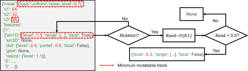
Figure 7: The configuration of a task in JSON style and the illustration of task mutation.

The configuration of a task is shown in Fig. 7. We introduce the detailed settings of different signal bases. (1) Noise is chosen from standard Gaussian distribution ($\mathcal{N}(0,1)$) or uniform distribution ($\mathcal{U}(-1,1)$). The generated noise maps are directly multiplied by the level which can be selected from 0 to 1 with a step of 0.1. (2) Sin1D generates 2D synthetic feature maps using different frequencies choosing from the range, which contains 10 frequencies sampled from $[a,b]$, where a and b are sampled from 0 to 0.5 with the constraint $0<a<b<0.5$. (3) Sin2D uses the similar setting as Sin1D, where both the $f_{x}$ and $f_{y}$ for a 2D feature map are sampled from the range. (4) ${C}_{i}$ can be selected from $\{16,32,48,64,96\}$. Other settings are already described in Section 3.1.2. During the mutation, each minimum mutatable block (including signal definitions and the number of channels) has 0.2 probability to be regenerated as shown in Fig. 7. For RNN settings, we search for both the input and output synthetic signal tensors. The dimension $d$ is chosen from $\{16,32,48,64,96\}$.

A.2.3 End-to-end NAS

In the end-to-end NAS, GenNAS is incorporated in the RE as the fitness function to explore the search space. For NASBench-101, the mutation rate for each vertice is $1/|v|$ where $|v|=7$. More details of the search space NASBench-101 can be found in the original paper [30]. For NASBench-201, the mutation rate for each edge is $1/|e|$ where $|e|=6$. More details of the search space NASBench-101 can be found in the original paper [35]. For NDS ResNet series, the sub search space consists of 25000 sampled architectures from the whole search space. We apply mutation in RE by randomly sampling 200 architectures from the sub search space and choosing the most similar architecture as the child. For NASBench-NLP, we follow the work [29] by using the graph2vec [73] features find the most similar architecture as the child.

A.3 Additional Experiments

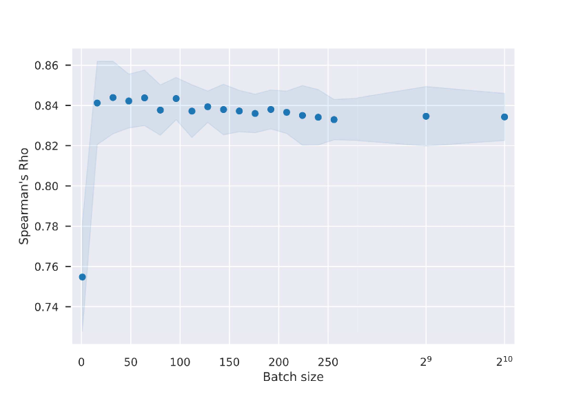
(a) Regression (GenNAS) ranking correlation averaged from 10 searched tasks using different batch sizes.

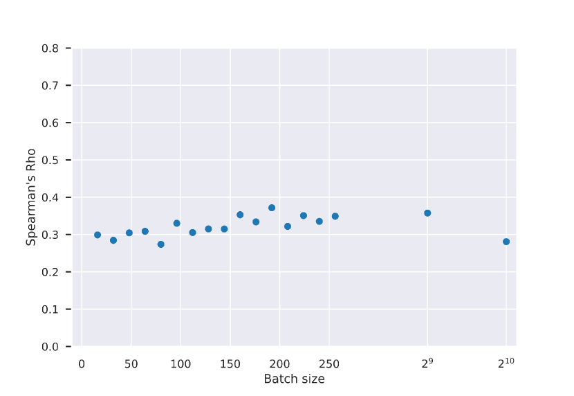
(b) Classification task’s ranking correlation using the same setting as (a).

(c) Classification accuracy vs. GenNS regression loss with batch size 1.

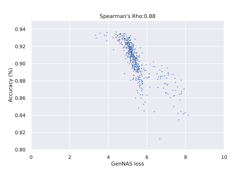
(d) Classification accuracy vs. GenNS regression loss with batch size 16.

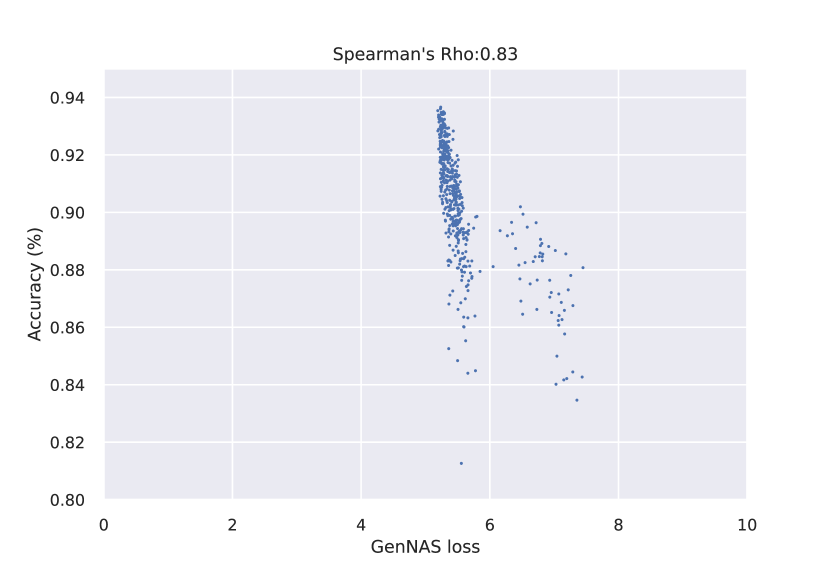
(e) Classification accuracy vs. GenNS regression loss with batch size 1024.

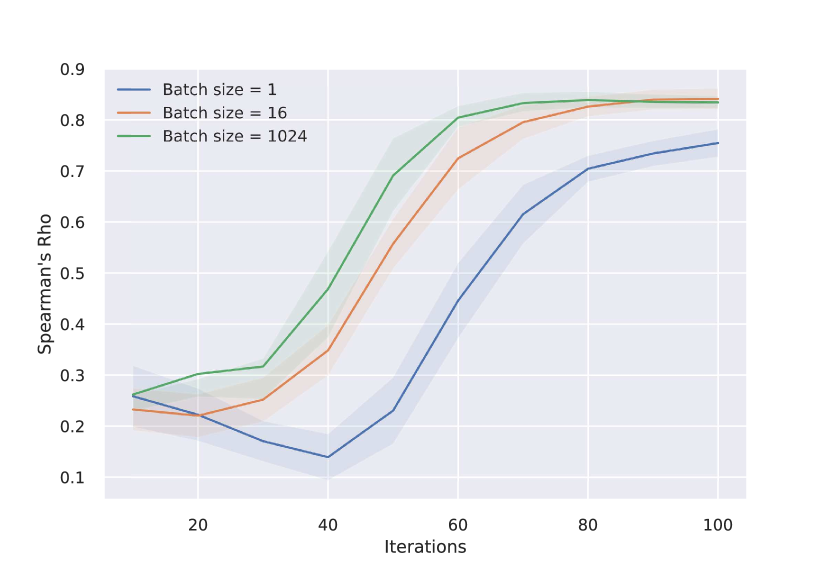
(f) 10 searched tasks’ ranking correlation on NASBench-101 using different numbers of iterations.

Figure 8: (a) Regression (GenNAS) ranking correlation averaged from 10 searched tasks on NASBench-101 in terms of Spearman’s $\rho$ with batch size in $\{1,16,32,...,256,512,1024\}$. (b) Classification task’s ranking correlation using the same amount of data in (a). (c) Classification accuracy using a searched task on NASBench-101 with batch size as 1 on CIFAR-10. The y-axis is the groundtruth (CIFAR-10 accuracy) and the x-axis is the GenNAS regression loss. (d) Similar to (c), batch size as 16. (e) Similar to (c), batch size as 1024. (f) 10 searched tasks ranking performance (in terms of Spearman’s $\rho$) on NASBench-101 using different iterations.

A.3.1 Regression vs. Classification Using Same Training Samples

We study effectiveness of regression using 10 tasks searched on NASBench-101, varying the batch size from 1 to 1024. The ranking correlation achieved by GenNAS using regression is plotted in Fig. 8(a). We also plot the classification task performances with single-batch data in Fig. 8(b). Apparently, using the same amount of data, the ranking correlation achieved by classification ($\rho$ around 0.85) is much worse than regression ($\rho$ around 0.3).

A.3.2 Batch Sizes and Iterations

We show the effect of batch size by using 10 tasks searched on NASBench-101. We use batch sizes varied from 1 to 1024 and plot the ranking results in Fig. 8(a). We find that 16 as the batch size is adequate for a good ranking performance. Also, we observe a small degradation when batch size increases and then becomes stable as the batch size keeps increasing. Hence, We plot the ranked architecture distribution with a searched task using 1, 16, 1024 as batch size respectively on Fig. 8(c), 8(d), 8(e). We observe that when only using a single image, the poor-performance architectures can also achieve similar regression losses as the good architectures. It suggests that the task is too easy to distinguish the differences among architectures. Also, 1024 as batch size leads to the higher regression losses of best architectures. It suggests that a very challenging task is also hard for good architectures to learn and may lead to slight ranking performance degradation. In addition, we plot the ranking performance using different numbers of iterations in Fig. 8(f). It shows that 100 iterations is necessary for the convergence of ranking performance.

A.3.3 Sensitivity Studies of Random Seeds and Initialization

Table 5: Ranking correlation (Spearman’s $\rho$) analysis of different 10 seeds across three different search spaces with the searched tasks on them respectively. For the NASBench-101, the 500 architecture samples [43] are constantly used for evaluation. For DARTS and ResNet search spaces, 1000 samples are randomly sampled with different seeds from the evaluated architecture sets provided by NDS [56].

Search Space	0	1	2	3	4	5	6	7	8	9	Average
NASBench-101	0.880	0.850	0.875	0.869	0.872	0.874	0.877	0.863	0.872	0.872	0.870$\pm$0.008
DARTS	0.809	0.899	0.861	0.831	0.841	0.836	0.851	0.841	0.885	0.861	0.850$\pm$0.025
ResNet	0.860	0.853	0.841	0.810	0.865	0.877	0.874	0.804	0.808	0.803	0.840$\pm$0.029

Random Seeds. We rerun the 3 searched tasks on their target search spaces (NASBench-101, DARTS, ResNet) for 10 runs with different random seeds. The results are shown in Table 5. GenNAS demonstrates its robustness across different random seeds.

Table 6: Ranking correlation (Spearman’s $\rho$) analysis of 10 searched tasks on NASBench-101 with different initialization methods.

Weight init	Bias init	0	1	2	3	4	5	6	7	8	9	Average
Default	Default	0.835	0.860	0.860	0.878	0.835	0.810	0.859	0.832	0.816	0.828	0.841$\pm$0.021
Kaiming	Default	0.844	0.854	0.857	0.856	0.832	0.818	0.854	0.746	0.829	0.811	0.830$\pm$0.032
Xavier	Default	0.856	0.881	0.863	0.874	0.849	0.825	0.865	0.830	0.838	0.851	0.853$\pm$0.018
Default	Zero	0.867	0.882	0.854	0.880	0.848	0.847	0.874	0.808	0.848	0.850	0.856$\pm$0.021
Kaiming	Zero	0.845	0.842	0.856	0.861	0.828	0.821	0.846	0.770	0.823	0.823	0.831$\pm$0.025
Xavier	Zero	0.859	0.876	0.869	0.879	0.839	0.842	0.861	0.828	0.846	0.843	0.854$\pm$0.016

Initialization. We perform an experiment to evaluate the effects of different initialization for 10 searched tasks on NASBench-101. For the weights, we use the default PyTorch initialization, Kaiming initialization [74], and Xavier initialization [75]. For the bias, we use the default PyTorch initialization and zeroized initialization. The results are shown in Table 6. We observe that for some specific tasks (e.g., task 7), Kaiming initialization may lead to lower ranking correlation. Also, zeroized bias initialization slightly increases the ranking correlation. However, overall, GenNAS shows stable performance across different initialization methods.

A.3.4 Kendall Tau and Retrieving Rates

For the sample experiments on NASBench-101/201/NLP and NDS, we report the performance of our methods compared to other efficient NAS approaches’ in Table 7 by Kendall $\tau$ [76]. We define the retrieving rate@topK as $\frac{\#\{\textnormal{Pred@TopK}\cap\textnormal{GT@TopK}\}}{\#\{\textnormal{GT@TopK}\}}$, where $\#$ is the operator of cardinality, GT@TopK and Pred@TopK are the set of architectures that are ranked in the top-K of groundtruths and predictions respectively. We report the retrieving rate@Top10% for all the search spaces in Table 8. Moreover, we report the retrieving rate@Top5%-Top50% for GenNAS-COMBO and GenNAS-N on NASBench-101 with other 1000 random sampled architectures in Table 9.

A.3.5 End-to-end NAS Architectures

Here we visualize all the ImageNet DARTS cell architectures: searched by GenNAS-combo, searched by GenNAS-D14 in Fig 9 and Fig 10 respectively.

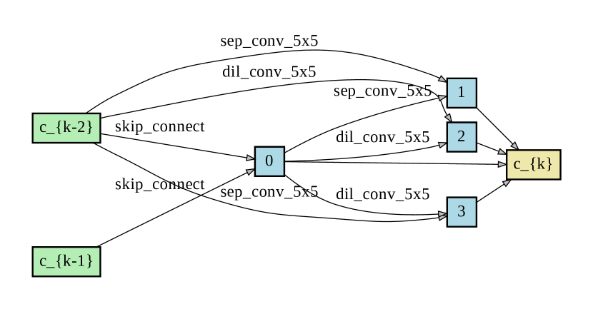
(a) Normal cell

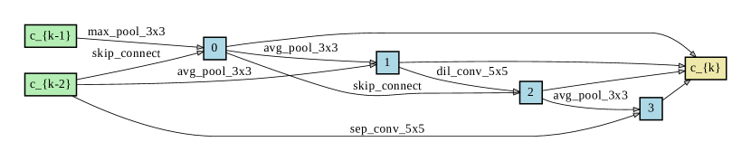
(b) Reduce cell

Figure 9: Cell architectures (normal and reduce) searched by GenNAS-combo

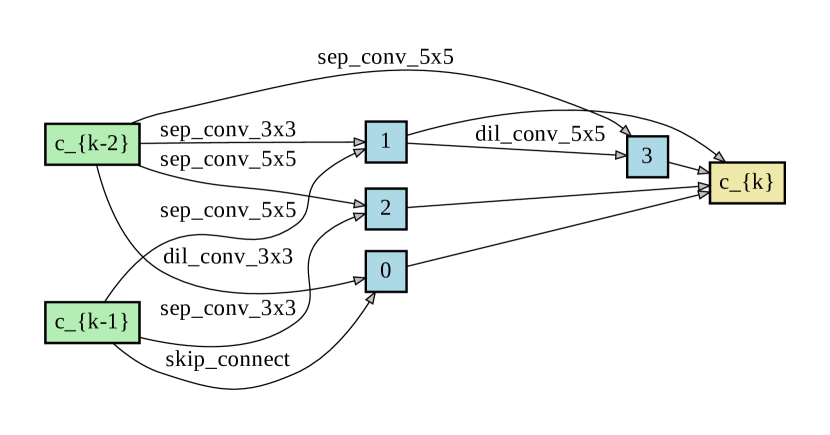
(a) Normal cell

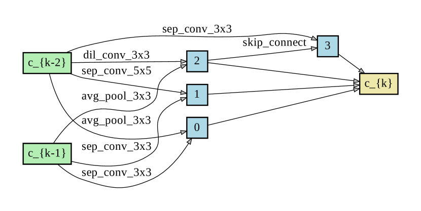
(b) Reduce cell

Figure 10: Cell architectures (normal and reduce) searched by GenNAS-D14

Table 7: GenNAS’ ranking correlation evaluation comparing with other efficient NAS approaches using the Kendall $\tau$.

NASBench-101
Dataset	NASWOT	synflow	GenNAS
	[37]	[31]	single	combo	search-N
CIFAR-10	0.27	0.24	0.59	0.66	0.7
ImgNet	0.36	0.14	0.47	0.54	0.53

NASBench-201
Dataset	NASWOT	synflow	jacob_cov	snip	EcoNAS	GenNAS
					[26]	single	combo	search-N
CIFAR-10	0.6	0.52	0.59	0.41	0.62	0.57	0.67	0.71
CIFAR-100	0.63	0.57	0.53	0.46	0.57	0.52	0.63	0.65
ImgNet16	0.6	0.54	0.56	0.44	0.57	0.53	0.61	0.67

Neural Design Spaces
Dataset	NAS-Space	NASWOT	synflow	GenNAS
				single	combo	search-N	search-D	search-R
CIFAR-10	DARTS	0.48	0.3	0.3	0.45	0.52	0.68	0.63
	DARTS-f	0.21	0.09	0.36	0.43	0.37	0.42	0.36
	Amoeba	0.21	0.06	0.36	0.47	0.5	0.59	0.53
	ENAS	0.39	0.13	0.39	0.49	0.48	0.63	0.59
	ENAS-f	0.31	0.2	0.46	0.55	0.49	0.53	0.48
	NASNet	0.3	0.02	0.4	0.5	0.47	0.58	0.52
	PNAS	0.36	0.17	0.22	0.37	0.42	0.57	0.52
	PNAS-f	0.09	0.18	0.31	0.38	0.39	0.38	0.33
	ResNet	0.19	0.14	0.23	0.38	0.38	0.38	0.64
	ResNeXt-A	0.46	0.32	0.4	0.5	0.6	0.45	0.65
	ResNeXt-B	0.4	0.43	0.17	0.3	0.37	0.38	0.52
ImageNet	DARTS	0.49	0.14	0.43	0.52	0.52	0.66	0.48
	DARTS-f	0.13	0.25	0.49	0.57	0.48	0.51	0.42
	Amoeba	0.33	0.17	0.46	0.53	0.55	0.62	0.5
	ENAS	0.51	0.12	0.4	0.47	0.4	0.63	0.48
	NASNet	0.39	0.01	0.36	0.42	0.37	0.5	0.43
	PNAS	0.45	0.11	0.19	0.27	0.31	0.45	0.3
	ResNeXt-A	0.52	0.28	0.61	0.7	0.56	0.44	0.69
	ResNeXt-B	0.45	0.21	0.53	0.65	0.39	0.43	0.67

NASBench-NLP
Dataset	GenNAS
	single	combo	search
PTB	0.43	0.55	0.63

Table 8: GenNAS’ retrieving rate@top10% comparing with other efficient NAS approaches. For the NASBench-101 we use the set of 500 architectures that sampled by Liu, et al. [43] for obtaining the ImageNet groundtruth.

NASBench-101
Dataset	number	NASWOT	synflow	GenNAS
	of samples	[37]	[31]	single	combo	search-N
CIFAR-10	500	32%	28%	58%	64%	68%
ImgNet	500	36%	14%	52%	54%	64%

NASBench-201
Dataset	number	NASWOT	synflow	jacob_cov	snip	EcoNAS	GenNAS
	of samples					[26]	single	combo	search-N
CIFAR-10	1000	43%	48%	27%	27%	52%	43%	36%	53%
CIFAR-100	1000	48%	47%	23%	36%	47%	46%	46%	58%
ImgNet16	1000	49%	43%	33%	32%	41%	48%	40%	51%

Neural Design Spaces
Dataset	number	NAS-Space	NASWOT	synflow	GenNAS
	of samples				single	combo	search-N	search-D	search-R
CIFAR-10	1000	DARTS	29%	10%	16%	43%	45%	59%	49%
	1000	DARTS-f	1%	5%	22%	33%	18%	22%	23%
	1000	Amoeba	20%	4%	20%	39%	45%	50%	40%
	1000	ENAS	31%	6%	25%	48%	41%	57%	48%
	1000	ENAS-f	28%	2%	34%	45%	42%	38%	37%
	1000	NASNet	33%	7%	27%	38%	46%	52%	43%
	1000	PNAS	24%	9%	21%	39%	46%	44%	37%
	1000	PNAS-f	6%	4%	21%	27%	31%	25%	22%
	1000	ResNet	7%	4%	38%	44%	38%	54%	64%
	1000	ResNeXt-A	28%	25%	25%	61%	53%	52%	58%
	1000	ResNeXt-B	21%	30%	10%	13%	36%	40%	71%
ImageNet	121	DARTS	17%	0%	50%	58%	55%	58%	18%
	499	DARTS-f	8%	4%	33%	27%	35%	39%	24%
	124	Amoeba	33%	0%	50%	42%	58%	58%	41%
	117	ENAS	36%	9%	18%	18%	45%	55%	45%
	122	NASNet	33%	0%	42%	50%	42%	33%	33%
	119	PNAS	10%	9%	45%	36%	45%	55%	9%
	130	ResNeXt-A	31%	8%	67%	67%	50%	33%	75%
	164	ResNeXt-B	38%	13%	38%	50%	33%	38%	64%

NASBench-NLP
Dataset	number	grad	norm	snip	grasp	fisher	synflow	GenNAS
	of samples							single	combo	search
PTB	1000	10%	10%	4%	-	22%	38%	38%	47%	63%

Table 9: Retrieving rate@top5%-top50% of GenNAS-combo/N on 1000 randomly sampled architectures on NASBench-101.

Method	@top5%	@top10%	@top20%	@top30%	@top40%	@top50%
GenNAS-combo	0.6	0.6	0.73	0.74	0.79	0.82
GenNAS-N	0.56	0.58	0.66	0.76	0.80	0.85

A.3.6 GPU Performance

We use the PyTorch 1.5.0 [77], on a desktop with I7-7700K CPU, 16 GB RAM and a GTX 1080 Ti GPU (11GB GDDR5X memory) to evaluate the GPU performance of GenNAS. The results are shown in Table 10.

Table 10: Evaluations of GenNAS’ GPU performance. We test GenNAS with 6 different batch sizes from 16 to 96. "A/B" denotes: A (second) as the average one-iteration run time for the search space, and B (GB or gigabyte) as the GPU memory usage. "OOM" means some large models may lead to the out-of-memory issue for the target GPU.

Search Space	B-size 16	B-size 32	B-size 48	B-size 64	B-size 80	B-size 96
NASBench-101	0.023/0.78	0.023/0.92	0.023/1.12	0.022/1.22	0.023/1.41	0.023/1.56
NASBench-201	0.020/0.77	0.020/0.93	0.021/1.12	0.020/1.24	0.020/1.46	0.020/1.62
DARTS	0.049/1.92	0.056/3.39	0.069/5.07	0.088/6.88	0.103/7.62	OOM
DARTS-f	0.077/1.42	0.088/2.21	0.104/3.30	0.122/3.79	0.145/5.15	0.171/6.07
Amoeba	0.080/2.53	0.103/4.38	0.128/6.60	0.159/9.25	0.194/6.85	OOM
ENAS	0.059/2.40	0.076/4.31	0.090/5.84	0.115/7.78	0.140/9.15	OOM
ENAS-f	0.095/1.67	0.111/2.58	0.134/3.70	0.159/4.54	0.186/6.31	0.216/7.53
NASNet	0.061/2.23	0.073/3.77	0.094/5.83	0.116/6.87	0.140/8.68	0.160/9.30
PNAS	0.074/2.52	0.097/4.36	0.121/6.53	0.155/8.23	0.189/9.42	OOM
PNAS-f	0.114/1.69	0.143/2.67	0.173/4.03	0.208/4.83	0.250/6.24	0.293/7.45
ResNet	0.016/1.28	0.016/1.54	0.016/2.05	0.016/2.34	0.016/2.34	0.016/2.77
ResNeXt-A	0.025/1.65	0.025/2.82	0.026/4.55	0.027/6.86	0.028/9.75	0.029/5.92
ResNeXt-B	0.022/1.98	0.022/3.47	0.023/5.63	0.024/7.33	0.027/9.51	0.029/5.95
NASBench-NLP	0.029/0.90	0.029/0.90	0.029/0.90	0.029/0.90	0.029/0.93	0.029/0.94

References

- [1] Esteban Real, Alok Aggarwal, Yanping Huang, and Quoc V Le. Regularized evolution for image classifier architecture search. In Proceedings of the aaai conference on artificial intelligence, volume 33, pages 4780–4789, 2019.
- [2] Barret Zoph and Quoc V Le. Neural architecture search with reinforcement learning. arXiv preprint arXiv:1611.01578, 2016.
- [3] Hanxiao Liu, Karen Simonyan, and Yiming Yang. Darts: Differentiable architecture search. arXiv preprint arXiv:1806.09055, 2018.
- [4] Han Cai, Ligeng Zhu, and Song Han. Proxylessnas: Direct neural architecture search on target task and hardware. arXiv preprint arXiv:1812.00332, 2018.
- [5] Xiu Su, Shan You, Jiyang Xie, Mingkai Zheng, Fei Wang, Chen Qian, Changshui Zhang, Xiaogang Wang, and Chang Xu. Vision transformer architecture search. arXiv preprint arXiv:2106.13700, 2021.
- [6] Chenxi Liu, Liang-Chieh Chen, Florian Schroff, Hartwig Adam, Wei Hua, Alan L Yuille, and Li Fei-Fei. Auto-deeplab: Hierarchical neural architecture search for semantic image segmentation. In Proceedings of the IEEE/CVF Conference on Computer Vision and Pattern Recognition, pages 82–92, 2019.
- [7] Vladimir Nekrasov, Hao Chen, Chunhua Shen, and Ian Reid. Fast neural architecture search of compact semantic segmentation models via auxiliary cells. In Proceedings of the IEEE/CVF Conference on Computer Vision and Pattern Recognition, pages 9126–9135, 2019.
- [8] Albert Shaw, Daniel Hunter, Forrest Landola, and Sammy Sidhu. Squeezenas: Fast neural architecture search for faster semantic segmentation. In Proceedings of the IEEE/CVF International Conference on Computer Vision Workshops, pages 0–0, 2019.
- [9] Changlin Li, Tao Tang, Guangrun Wang, Jiefeng Peng, Bing Wang, Xiaodan Liang, and Xiaojun Chang. Bossnas: Exploring hybrid cnn-transformers with block-wisely self-supervised neural architecture search. arXiv preprint arXiv:2103.12424, 2021.
- [10] Hanrui Wang, Zhanghao Wu, Zhijian Liu, Han Cai, Ligeng Zhu, Chuang Gan, and Song Han. Hat: Hardware-aware transformers for efficient natural language processing. arXiv preprint arXiv:2005.14187, 2020.
- [11] David So, Quoc Le, and Chen Liang. The evolved transformer. In International Conference on Machine Learning, pages 5877–5886. PMLR, 2019.
- [12] Cong Hao and Deming Chen. Deep neural network model and fpga accelerator co-design: Opportunities and challenges. In 2018 14th IEEE International Conference on Solid-State and Integrated Circuit Technology (ICSICT), pages 1–4. IEEE, 2018.
- [13] Cong Hao, Xiaofan Zhang, Yuhong Li, Sitao Huang, Jinjun Xiong, Kyle Rupnow, Wen-mei Hwu, and Deming Chen. Fpga/dnn co-design: An efficient design methodology for 1ot intelligence on the edge. In 2019 56th ACM/IEEE Design Automation Conference (DAC), pages 1–6. IEEE, 2019.
- [14] Xiaofan Zhang, Haoming Lu, Cong Hao, Jiachen Li, Bowen Cheng, Yuhong Li, Kyle Rupnow, Jinjun Xiong, Thomas Huang, Honghui Shi, et al. Skynet: a hardware-efficient method for object detection and tracking on embedded systems. arXiv preprint arXiv:1909.09709, 2019.
- [15] Ji Lin, Wei-Ming Chen, Yujun Lin, John Cohn, Chuang Gan, and Song Han. Mcunet: Tiny deep learning on iot devices. arXiv preprint arXiv:2007.10319, 2020.
- [16] Ji Lin, Wei-Ming Chen, Han Cai, Chuang Gan, and Song Han. Mcunetv2: Memory-efficient patch-based inference for tiny deep learning. arXiv preprint arXiv:2110.15352, 2021.
- [17] Esteban Real, Sherry Moore, Andrew Selle, Saurabh Saxena, Yutaka Leon Suematsu, Jie Tan, Quoc V Le, and Alexey Kurakin. Large-scale evolution of image classifiers. In International Conference on Machine Learning, pages 2902–2911. PMLR, 2017.
- [18] Barret Zoph, Vijay Vasudevan, Jonathon Shlens, and Quoc V Le. Learning transferable architectures for scalable image recognition. In Proceedings of the IEEE conference on computer vision and pattern recognition, pages 8697–8710, 2018.
- [19] Kaiming He, Xiangyu Zhang, Shaoqing Ren, and Jian Sun. Deep residual learning for image recognition. In Proceedings of the IEEE conference on computer vision and pattern recognition, pages 770–778, 2016.
- [20] Liang-Chieh Chen, Yukun Zhu, George Papandreou, Florian Schroff, and Hartwig Adam. Encoder-decoder with atrous separable convolution for semantic image segmentation. In Proceedings of the European conference on computer vision (ECCV), pages 801–818, 2018.
- [21] Mark Marsden, Kevin McGuinness, Suzanne Little, and Noel E O’Connor. Resnetcrowd: A residual deep learning architecture for crowd counting, violent behaviour detection and crowd density level classification. In 2017 14th IEEE International Conference on Advanced Video and Signal Based Surveillance (AVSS), pages 1–7. IEEE, 2017.
- [22] Maithra Raghu, Chiyuan Zhang, Jon Kleinberg, and Samy Bengio. Transfusion: Understanding transfer learning for medical imaging. arXiv preprint arXiv:1902.07208, 2019.
- [23] Marti A. Hearst, Susan T Dumais, Edgar Osuna, John Platt, and Bernhard Scholkopf. Support vector machines. IEEE Intelligent Systems and their applications, 13(4):18–28, 1998.
- [24] Arthur Jacot, Franck Gabriel, and Clément Hongler. Neural tangent kernel: Convergence and generalization in neural networks. arXiv preprint arXiv:1806.07572, 2018.
- [25] Wayne W Daniel et al. Applied nonparametric statistics. 1990.
- [26] Dongzhan Zhou, Xinchi Zhou, Wenwei Zhang, Chen Change Loy, Shuai Yi, Xuesen Zhang, and Wanli Ouyang. Econas: Finding proxies for economical neural architecture search. In Proceedings of the IEEE/CVF Conference on Computer Vision and Pattern Recognition, pages 11396–11404, 2020.
- [27] Xiangxiang Chu, Bo Zhang, Ruijun Xu, and Jixiang Li. Fairnas: Rethinking evaluation fairness of weight sharing neural architecture search. arXiv preprint arXiv:1907.01845, 2019.
- [28] Liam Li and Ameet Talwalkar. Random search and reproducibility for neural architecture search. In Uncertainty in Artificial Intelligence, pages 367–377. PMLR, 2020.
- [29] Nikita Klyuchnikov, Ilya Trofimov, Ekaterina Artemova, Mikhail Salnikov, Maxim Fedorov, and Evgeny Burnaev. Nas-bench-nlp: neural architecture search benchmark for natural language processing. arXiv preprint arXiv:2006.07116, 2020.
- [30] Chris Ying, Aaron Klein, Eric Christiansen, Esteban Real, Kevin Murphy, and Frank Hutter. Nas-bench-101: Towards reproducible neural architecture search. In International Conference on Machine Learning, pages 7105–7114. PMLR, 2019.
- [31] Mohamed S Abdelfattah, Abhinav Mehrotra, Łukasz Dudziak, and Nicholas D Lane. Zero-cost proxies for lightweight nas. arXiv preprint arXiv:2101.08134, 2021.
- [32] Yuhui Xu, Lingxi Xie, Xiaopeng Zhang, Xin Chen, Guo-Jun Qi, Qi Tian, and Hongkai Xiong. Pc-darts: Partial channel connections for memory-efficient architecture search. arXiv preprint arXiv:1907.05737, 2019.
- [33] Yuhong Li, Cong Hao, Xiaofan Zhang, Xinheng Liu, Yao Chen, Jinjun Xiong, Wen-mei Hwu, and Deming Chen. Edd: Efficient differentiable dnn architecture and implementation co-search for embedded ai solutions. In 2020 57th ACM/IEEE Design Automation Conference (DAC), pages 1–6. IEEE, 2020.
- [34] Arber Zela, Thomas Elsken, Tonmoy Saikia, Yassine Marrakchi, Thomas Brox, and Frank Hutter. Understanding and robustifying differentiable architecture search. arXiv preprint arXiv:1909.09656, 2019.
- [35] Xuanyi Dong and Yi Yang. Nas-bench-201: Extending the scope of reproducible neural architecture search. arXiv preprint arXiv:2001.00326, 2020.
- [36] Kaicheng Yu, Christian Sciuto, Martin Jaggi, Claudiu Musat, and Mathieu Salzmann. Evaluating the search phase of neural architecture search. arXiv preprint arXiv:1902.08142, 2019.
- [37] Joseph Mellor, Jack Turner, Amos Storkey, and Elliot J Crowley. Neural architecture search without training. arXiv preprint arXiv:2006.04647, 2020.
- [38] Debadeepta Dey, Shital Shah, and Sebastien Bubeck. Fear: A simple lightweight method to rank architectures. arXiv preprint arXiv:2106.04010, 2021.
- [39] Guihong Li, Sumit K Mandal, Umit Y Ogras, and Radu Marculescu. Flash: Fast neural architecture search with hardware optimization. ACM Transactions on Embedded Computing Systems (TECS), 20(5s):1–26, 2021.
- [40] Julien Siems, Lucas Zimmer, Arber Zela, Jovita Lukasik, Margret Keuper, and Frank Hutter. Nas-bench-301 and the case for surrogate benchmarks for neural architecture search. arXiv preprint arXiv:2008.09777, 2020.
- [41] Xiu Su, Tao Huang, Yanxi Li, Shan You, Fei Wang, Chen Qian, Changshui Zhang, and Chang Xu. Prioritized architecture sampling with monto-carlo tree search. In Proceedings of the IEEE/CVF Conference on Computer Vision and Pattern Recognition, pages 10968–10977, 2021.
- [42] Simon Kornblith, Jonathon Shlens, and Quoc V Le. Do better imagenet models transfer better? In Proceedings of the IEEE/CVF Conference on Computer Vision and Pattern Recognition, pages 2661–2671, 2019.
- [43] Chenxi Liu, Piotr Dollár, Kaiming He, Ross Girshick, Alan Yuille, and Saining Xie. Are labels necessary for neural architecture search? In European Conference on Computer Vision, pages 798–813. Springer, 2020.
- [44] Longlong Jing and Yingli Tian. Self-supervised visual feature learning with deep neural networks: A survey. IEEE Transactions on Pattern Analysis and Machine Intelligence, 2020.
- [45] Alexey Dosovitskiy, Jost Tobias Springenberg, Martin Riedmiller, and Thomas Brox. Discriminative unsupervised feature learning with convolutional neural networks. Citeseer, 2014.
- [46] Carl Doersch, Abhinav Gupta, and Alexei A Efros. Unsupervised visual representation learning by context prediction. In Proceedings of the IEEE international conference on computer vision, pages 1422–1430, 2015.
- [47] Xiaolong Wang and Abhinav Gupta. Unsupervised learning of visual representations using videos. In Proceedings of the IEEE international conference on computer vision, pages 2794–2802, 2015.
- [48] Haohan Wang, Xindi Wu, Zeyi Huang, and Eric P Xing. High-frequency component helps explain the generalization of convolutional neural networks. In Proceedings of the IEEE/CVF Conference on Computer Vision and Pattern Recognition, pages 8684–8694, 2020.
- [49] Jonathan Long, Evan Shelhamer, and Trevor Darrell. Fully convolutional networks for semantic segmentation. In Proceedings of the IEEE conference on computer vision and pattern recognition, pages 3431–3440, 2015.
- [50] Sepp Hochreiter and Jürgen Schmidhuber. Long short-term memory. Neural computation, 9(8):1735–1780, 1997.
- [51] Tomáš Mikolov, Martin Karafiát, Lukáš Burget, Jan Černockỳ, and Sanjeev Khudanpur. Recurrent neural network based language model. In Eleventh annual conference of the international speech communication association, 2010.
- [52] Ashish Vaswani, Noam Shazeer, Niki Parmar, Jakob Uszkoreit, Llion Jones, Aidan N Gomez, Lukasz Kaiser, and Illia Polosukhin. Attention is all you need. arXiv preprint arXiv:1706.03762, 2017.
- [53] Zhi-Qin John Xu, Yaoyu Zhang, Tao Luo, Yanyang Xiao, and Zheng Ma. Frequency principle: Fourier analysis sheds light on deep neural networks. arXiv preprint arXiv:1901.06523, 2019.
- [54] Georgi P Tolstov. Fourier series. Courier Corporation, 2012.
- [55] Stephen J Montgomery-Smith. The distribution of rademacher sums. Proceedings of the American Mathematical Society, 109(2):517–522, 1990.
- [56] Ilija Radosavovic, Justin Johnson, Saining Xie, Wan-Yen Lo, and Piotr Dollár. On network design spaces for visual recognition. In Proceedings of the IEEE/CVF International Conference on Computer Vision, pages 1882–1890, 2019.
- [57] Mitchell Marcus, Beatrice Santorini, and Mary Ann Marcinkiewicz. Building a large annotated corpus of english: The penn treebank. 1993.
- [58] Xuanyi Dong and Yi Yang. Searching for a robust neural architecture in four gpu hours. In Proceedings of the IEEE/CVF Conference on Computer Vision and Pattern Recognition, pages 1761–1770, 2019.
- [59] Xuanyi Dong and Yi Yang. One-shot neural architecture search via self-evaluated template network. In Proceedings of the IEEE/CVF International Conference on Computer Vision, pages 3681–3690, 2019.
- [60] Hieu Pham, Melody Guan, Barret Zoph, Quoc Le, and Jeff Dean. Efficient neural architecture search via parameters sharing. In International Conference on Machine Learning, pages 4095–4104. PMLR, 2018.
- [61] Jia Deng, Wei Dong, Richard Socher, Li-Jia Li, Kai Li, and Li Fei-Fei. Imagenet: A large-scale hierarchical image database. In 2009 IEEE conference on computer vision and pattern recognition, pages 248–255. Ieee, 2009.
- [62] Wuyang Chen, Xinyu Gong, and Zhangyang Wang. Neural architecture search on imagenet in four gpu hours: A theoretically inspired perspective. arXiv preprint arXiv:2102.11535, 2021.
- [63] Chenxi Liu, Barret Zoph, Maxim Neumann, Jonathon Shlens, Wei Hua, Li-Jia Li, Li Fei-Fei, Alan Yuille, Jonathan Huang, and Kevin Murphy. Progressive neural architecture search. In Proceedings of the European conference on computer vision (ECCV), pages 19–34, 2018.
- [64] Sirui Xie, Hehui Zheng, Chunxiao Liu, and Liang Lin. Snas: stochastic neural architecture search. arXiv preprint arXiv:1812.09926, 2018.
- [65] Xin Chen, Lingxi Xie, Jun Wu, and Qi Tian. Progressive differentiable architecture search: Bridging the depth gap between search and evaluation. In Proceedings of the IEEE/CVF International Conference on Computer Vision, pages 1294–1303, 2019.
- [66] Volodymyr Kindratenko, Dawei Mu, Yan Zhan, John Maloney, Sayed Hadi Hashemi, Benjamin Rabe, Ke Xu, Roy Campbell, Jian Peng, and William Gropp. Hal: Computer system for scalable deep learning. In Practice and Experience in Advanced Research Computing, pages 41–48. 2020.
- [67] Ilija Radosavovic, Raj Prateek Kosaraju, Ross Girshick, Kaiming He, and Piotr Dollár. Designing network design spaces. In CVPR, 2020.
- [68] Saining Xie, Ross Girshick, Piotr Dollár, Zhuowen Tu, and Kaiming He. Aggregated residual transformations for deep neural networks. In Proceedings of the IEEE conference on computer vision and pattern recognition, pages 1492–1500, 2017.
- [69] Ilya Sutskever, James Martens, George Dahl, and Geoffrey Hinton. On the importance of initialization and momentum in deep learning. In International conference on machine learning, pages 1139–1147. PMLR, 2013.
- [70] Diederik P Kingma and Jimmy Ba. Adam: A method for stochastic optimization. arXiv preprint arXiv:1412.6980, 2014.
- [71] David E Goldberg and Kalyanmoy Deb. A comparative analysis of selection schemes used in genetic algorithms. In Foundations of genetic algorithms, volume 1, pages 69–93. Elsevier, 1991.
- [72] Yukang Chen, Gaofeng Meng, Qian Zhang, Shiming Xiang, Chang Huang, Lisen Mu, and Xinggang Wang. Renas: Reinforced evolutionary neural architecture search. In Proceedings of the IEEE/CVF Conference on Computer Vision and Pattern Recognition, pages 4787–4796, 2019.
- [73] Annamalai Narayanan, Mahinthan Chandramohan, Rajasekar Venkatesan, Lihui Chen, Yang Liu, and Shantanu Jaiswal. graph2vec: Learning distributed representations of graphs. arXiv preprint arXiv:1707.05005, 2017.
- [74] Kaiming He, Xiangyu Zhang, Shaoqing Ren, and Jian Sun. Delving deep into rectifiers: Surpassing human-level performance on imagenet classification. In Proceedings of the IEEE international conference on computer vision, pages 1026–1034, 2015.
- [75] Xavier Glorot and Yoshua Bengio. Understanding the difficulty of training deep feedforward neural networks. In Proceedings of the thirteenth international conference on artificial intelligence and statistics, pages 249–256. JMLR Workshop and Conference Proceedings, 2010.
- [76] Maurice G Kendall. A new measure of rank correlation. Biometrika, 30(1/2):81–93, 1938.
- [77] Adam Paszke, Sam Gross, Francisco Massa, Adam Lerer, James Bradbury, Gregory Chanan, Trevor Killeen, Zeming Lin, Natalia Gimelshein, Luca Antiga, Alban Desmaison, Andreas Kopf, Edward Yang, Zachary DeVito, Martin Raison, Alykhan Tejani, Sasank Chilamkurthy, Benoit Steiner, Lu Fang, Junjie Bai, and Soumith Chintala. Pytorch: An imperative style, high-performance deep learning library. In H. Wallach, H. Larochelle, A. Beygelzimer, F. d'Alché-Buc, E. Fox, and R. Garnett, editors, Advances in Neural Information Processing Systems 32, pages 8024–8035. Curran Associates, Inc., 2019.