On the Parameter Estimation in the Schwartz-Smith’s Two-Factor Model

Abstract

The two unobservable state variables representing the short and long term factors introduced by Schwartz and Smith in [16] for risk-neutral pricing of futures contracts are modelled as two correlated Ornstein-Uhlenbeck processes. The Kalman Filter (KF) method has been implemented to estimate the “short” and “long” term factors jointly with unknown model parameters. The parameter identification problem arising within the likelihood function in the KF has been addressed by introducing an additional constraint. The obtained model parameter estimates are the conditional Maximum Likelihood Estimators (MLEs) evaluated within the KF. Consistency of the conditional MLEs is studied. The methodology has been tested on simulated data.

1 Introduction

Over more than four decades stochastic processes have been used for modelling of commodity futures prices. In early studies, the commodity prices were modelled using a geometric Brownian motion, [3]. For pricing of commodity derivatives, the mean-reverting processes were used for the first time in [8]; they are also known as Ornstein-Uhlenbeck (O-U) processes, primarily introduced in [14] for modelling of velocity process of Brownian particle under friction.

This work is based on the paper by Schwartz and Smith in [16], where the O-U two-factor model was used for modelling of short and long equilibrium commodity spot price levels. A commodity spot price $S_{t}$ is modelled as the sum of two unobservable factors $\chi_{t}$ and $\xi_{t}$. Both processes $\chi_{t}$ and $\xi_{t}$ are represented as the mean-reverting processes. In the mean-reverting model, when the commodity price is higher than the equilibrium price level, some new suppliers will enter the market and create downward pressure on the prices. Conversely, when the price is lower than the equilibrium price level, some high-cost suppliers will exit the market and put upward pressure on the prices. In the short term, due to these movements, the price fluctuates temporarily, and it will eventually converge to its equilibrium level over the long term.

Kalman’s filtering technique for estimation of the state variables using historical futures prices remains popular for its ability to reproduce realistic commodity futures term structure, see e.g. [1]. In [5], the authors improved the performance of the Kalman Filter by deriving the commodity spot prices from futures prices which have had incorporated an analyst’s forecasts of spot prices. In [4], the Kalman Filter is used to study the effect of stochastic volatility and interest rates on the commodity spot prices using the market prices of long-dated futures and options. The Kalman technique was used in [15] for calibration and filtering of partially observable processes using particle Markov chain Monte Carlo approach. The authors of [6] developed the extended Kalman Filter for estimation of the state variables in the two-factor model for the commodity spot price and its yield developed in [17].

Our motivation is driven by the fact that the parameter estimation problem in the linear system using the Kalman Filter cannot be overlooked whilst the estimation of the state variables remains the priority. In the different setup the parameter estimation problem for bivariate O-U process using Kalman Filter has been studied in [7, 13].

In this paper, we conduct the simulation study where the Kalman Filter is deployed for estimation of the model parameters jointly with the components of the logarithm of spot price processs, which is used in the pricing formula for the futures contracts. In Section 2, we provide the notation and analytical formulae used for the formulation of linear partially observable system specific for commodity futures pricing given in [16]. In Section 3, we present the details of our implementation of KF algorithm designed for estimation of the parameters of the multi-dimensional partially observable linear system jointly with the estimation of unobserved state variables $\chi_{t}$ and $\xi_{t}$. The results of the simulation study are presented in Section 4.

2 Two-Factor Model

In this section, we provide a brief description of Schwartz-Smith’s model from [16]. We discuss the risk-neutral setup used for futures pricing and present the formulae for futures prices, incorporating the short and long term dynamic factors.

2.1 A Commodity Spot Price Modelling

We model the logarithm of the spot price $S_{t}$ using the additive model,

$$\log(S_{t})=\chi_{t}+\xi_{t},$$

where $\chi_{t}$ and $\xi_{t}$ are the short and long dynamic factors, respectively. We assume that changes in $\chi_{t}$ are temporary and it converges to 0 in a long term, following an O-U process

$$d\chi_{t}=-\kappa\chi_{t}dt+\sigma_{\chi}dZ_{t}^{\chi},$$

with the mean 0. The changes in the equilibrium level of $\xi_{t}$ are expected to persist and the process itself is assumed to be mean-reverting

$$d\xi_{t}=(\mu_{\xi}-\gamma\xi_{t})dt+\sigma_{\xi}dZ_{t}^{\xi}.$$

The processes $Z_{t}^{\chi}$ and $Z_{t}^{\xi}$ are correlated standard Brownian motions with
$dZ_{t}^{\chi}dZ_{t}^{\xi}=\rho_{\chi\xi}dt$, and $\rho=\rho_{\chi\xi}$. Given the initial values $\chi_{0}$ and $\xi_{0}$, $\chi_{t}$ and $\xi_{t}$ are jointly normally distributed with expected value

$$E[(\chi_{t},\xi_{t})]=(e^{-\kappa t}\chi_{0},\frac{\mu_{\xi}}{\gamma}(1-e^{-\gamma t})+e^{-\gamma t}\xi_{0}),t\geq 0$$ (1)

and covariance matrix

$$Cov[(\chi_{t},\xi_{t})]=\left(\begin{array}[]{cc}\frac{1-e^{-2\kappa t}}{2\kappa}\sigma_{\chi}^{2}&\frac{1-e^{-(\kappa+\gamma)t}}{\kappa+\gamma}\sigma_{\chi}\sigma_{\xi}\rho_{\chi\xi}\\ \frac{1-e^{-(\kappa+\gamma)t}}{\kappa+\gamma}\sigma_{\chi}\sigma_{\xi}\rho_{\chi\xi}&\frac{1-e^{-2\gamma t}}{2\gamma}\sigma_{\xi}^{2}\end{array}\right).$$ (2)

Derivations of (1) and (2) are given in Appendix 0.A. Therefore, the logarithm of the spot price is normally distributed with mean

$$E[\log(S_{t})]=e^{-\kappa t}\chi_{0}+\frac{\mu_{\xi}}{\gamma}(1-e^{-\gamma t})+e^{-\gamma t}\xi_{0}$$

and variance

$$Var[\log(S_{t})]=\frac{1-e^{-2\kappa t}}{2\kappa}\sigma_{\chi}^{2}+\frac{1-e^{-2\gamma t}}{2\gamma}\sigma_{\xi}^{2}+2\frac{1-e^{-(\kappa+\gamma)t}}{\kappa+\gamma}\sigma_{\chi}\sigma_{\xi}\rho_{\chi\xi}.$$

Hence $S_{t}$, the commodity spot price, is log-normally distributed and

$$E(S_{t})=\exp(E[\log(S_{t})]+\frac{1}{2}Var[\log(S_{t})]),$$

or

$$\log[E(S_{t})]=e^{-\kappa t}\chi_{0}+\frac{\mu_{\xi}}{\gamma}(1-e^{-\gamma t})+e^{-\gamma t}\xi_{0}+$$

$$\frac{1}{2}\left(\frac{1-e^{-2\kappa t}}{2\kappa}\sigma_{\chi}^{2}+\frac{1-e^{-2\gamma t}}{2\gamma}\sigma_{\xi}^{2}+2\frac{1-e^{-(\kappa+\gamma)t}}{\kappa+\gamma}\sigma_{\chi}\sigma_{\xi}\rho_{\chi\xi}\right),$$ (3)

where $\frac{\mu_{\xi}}{\gamma}$ is the mean parameter, $\sigma_{\chi}$ and $\sigma_{\xi}$ are the volatilities, $\gamma$ and $\kappa$ are so-called the speed of mean-reversion parameters of $\chi$ and $\xi$ processes, respectively.

2.2 Risk-Neutral Approach to Spot Price Modelling

In this section we introduce two additional parameters which can be interpreted as the market price of commodity spot price risk. The approach stems from the risk-neutral pricing theory for futures, developed in [3]. Hence, the Schwartz-Smith’s model with additional parameters can be rewritten as follows

$$d\chi_{t}=(-\kappa\chi_{t}-\lambda_{\chi})dt+\sigma_{\chi}dZ_{t}^{\chi^{*}},$$

$$d\xi_{t}=(\mu_{\xi}-\gamma\xi_{t}-\lambda_{\xi})dt+\sigma_{\xi}dZ_{t}^{\xi^{*}},$$

where the parameters $\lambda_{\chi}$ and $\lambda_{\xi}$ appear as the risk-neutral mean correction terms. Under the risk-neutral measure, $\chi_{t}$ and $\xi_{t}$ are also jointly normally distributed with mean

$$E^{*}[(\chi_{t},\xi_{t})]=(e^{-\kappa t}\chi_{0}-\frac{\lambda_{\chi}}{\kappa}(1-e^{-\kappa t}),\frac{\mu_{\xi}-\lambda_{\xi}}{\gamma}(1-e^{-\gamma t})+e^{-\gamma t}\xi_{0})$$

and covariance matrix

$$Cov[(\chi_{t},\xi_{t})]^{*}=Cov[(\chi_{t},\xi_{t})].$$

The logarithm of commodity spot price is normally distributed with mean

$$E^{*}[\log(S_{t})]=e^{-\kappa t}\chi_{0}-\frac{\lambda_{\chi}}{\kappa}(1-e^{-\kappa t})+\frac{\mu_{\xi}-\lambda_{\xi}}{\gamma}(1-e^{-\gamma t})+e^{-\gamma t}\xi_{0}$$

and variance

$$Var^{*}[\log(S_{t})]=Var[\log(S_{t})].$$

The spot price is log-normally distributed with

$$\log[E^{*}(S_{t})]=E^{*}[\log(S_{t})]+\frac{1}{2}Var^{*}[\log(S_{t})]=e^{-\kappa t}\chi_{0}+e^{-\gamma t}\xi_{0}+A(t),$$ (4)

where

$$A(t)=-\frac{\lambda_{\chi}}{\kappa}(1-e^{-\kappa t})+\frac{\mu_{\xi}-\lambda_{\xi}}{\gamma}(1-e^{-\gamma t})+$$

$$\frac{1}{2}\left(\frac{1-e^{-2\kappa t}}{2\kappa}\sigma_{\chi}^{2}+\frac{1-e^{-2\gamma t}}{2\gamma}\sigma_{\xi}^{2}+2\frac{1-e^{-(\kappa+\gamma)t}}{\kappa+\gamma}\sigma_{\chi}\sigma_{\xi}\rho_{\chi\xi}\right).$$

In (4) the parameters $\lambda_{\chi}$ and $\lambda_{\xi}$ appear due to the adjustment made in (3).

2.3 Risk-Neutral Approach to Pricing of Futures

A futures contract is defined as an agreement to trade or own an asset in the future, [12]. We are interested to know what is the price of such contract at present. Let $F_{0,T}$ be the current market price of the futures contract with maturity $T$. For elimination of arbitrage, colloquially known as a “free-lunch”, the futures price must be equal to the expected commodity spot price at its delivery time $T$. Hence, under the risk-neutral measure from Section 2.2, assuming zero interest rate, we obtain

$$\log(F_{0,T})=\log[E^{*}(S_{T})]=e^{-\kappa T}\chi_{0}+e^{-\gamma T}\xi_{0}+A(T).$$

We denote

$$x_{t}=\left(\begin{matrix}\chi_{t}\\ \xi_{t}\end{matrix}\right),\;\;c=\left(\begin{array}[]{c}0\\ \frac{\mu_{\xi}}{\gamma}(1-e^{-\gamma\Delta t})\end{array}\right),\;\;G=\left(\begin{array}[]{cc}e^{-\kappa\Delta t}&0\\ 0&e^{-\gamma\Delta t}\end{array}\right),$$

$\Delta t$ is the discretization width.
Let $w_{t}$ be a column-vector of normally distributed random variables,

$$E(w_{t})=0$$

and

$$W=Cov(w_{t})=Cov[(\chi_{\Delta t},\xi_{\Delta t})].$$

In discrete time, we will obtain the following AR(1) dynamics for the bivariate state variable $x_{t}$

$$x_{t}=c+Gx_{t-1}+w_{t}.$$ (5)

The relationship between $x_{t}$ and the observed futures prices is given by

$$y_{t}=d_{t}+F_{t}^{\prime}x_{t}+v_{t},$$ (6)

where

$$y_{t}^{\prime}=(\log(F_{T_{1}}),\log(F_{T_{2}}),\dots,\log(F_{T_{n}})),$$

$$d_{t}^{\prime}=(A(T_{1}),A(T_{2}),\dots),A(T_{n}),$$

$$F_{t}=\begin{pmatrix}e^{-\kappa(T_{1}-t)},e^{-\kappa(T_{2}-t)},\dots,e^{-\kappa(T_{n}-t)}\\ e^{-\gamma(T_{1}-t)},e^{-\gamma(T_{2}-t)},\dots,e^{-\gamma(T_{n}-t)}\end{pmatrix},$$

and $v_{t}$ is a $n\times 1$ vector of independent, normally distributed random variables $E(v_{t})=0$ and $Cov(v_{t})=V$ and $T_{1},T_{2},...,T_{n}$ are the futures maturity times. We assume that $V$ is a diagonal matrix with the vector $v=(s_{1}^{2},s_{2}^{2},\dots,s_{n}^{2})$ of non-zero elements on the diagonal. The number of the futures contracts is $n$. Let $\mathcal{F}_{t}$ be a $\sigma$-algebra generated by the futures contracts up to time $t$ and $\theta=(\kappa,\gamma,\mu_{\xi},\sigma_{\chi},\sigma_{\xi},\rho,\lambda_{\chi},\lambda_{\xi},v)$ be a vector of unknown parameters. The model (5) - (6) is similar to the model discussed in Chapter 3, [10].

The conditional log-likelihood function of $y=(y_{1},y_{2},\dots,y_{n_{T}})$ is

$$l(\theta;y)=\sum_{t=1}^{n_{T}}p(y_{t}|\mathcal{F}_{t-1}),$$

where $p(y_{t}|\mathcal{F}_{t-1})$ is the probability density of $y_{t}$ given the information available until $t-1=t-\Delta$ and $n_{T}$ is the number of time-points. We assume that the prediction errors $e_{t}=y_{t}-E(y_{t}|\mathcal{F}_{t-1})$ have a multivariate normal distribution, then the log-likelihood function is

$$l(\theta;y)=-\frac{nn_{T}\log(2\pi)}{2}-\frac{1}{2}\sum_{t=1}^{n_{T}}[\log(\det(L_{t|t-1}))+e_{t}^{\prime}L_{t|t-1}^{-1}e_{t}]$$ (7)

where $L_{t|t-1}=Cov(e_{t}|\mathcal{F}_{t-1})$. The vector of unknown parameters $\theta$ will be estimated by maximising the log-likelihood function from (7). However, the maximisation of $l(\theta;y)$ is inhibited by the parameter identification problem. This fact can be proved analyticaly by mathematical induction since the prediction error $e_{t}$ and covariance matrix $L_{t|t-1}$ are invariant to label switching of coordinates of $x_{t}$.

3 Kalman Filter

In this section, we are using Kalman Filter to estimate the unobservable vector of state variables $x_{t}=(\chi_{t},\xi_{t})^{\prime}$ using simulated $y_{t}$. We recall the equations (5) and (6) for $x_{t}$ and $y_{t}$, respectively

$$x_{t}=c+Gx_{t-1}+w_{t},$$

$$y_{t}=d_{t}+F_{t}^{\prime}x_{t}+v_{t}.$$

For initialisation of the Kalman Filter we use the expectation and covariance matrix, suggested in [2]

$$a_{0}=E(x_{0})=\left(0,\frac{\mu_{\xi}}{\gamma}\right)^{\prime}$$

and

$$P_{0}=Cov(x_{0})=\left(\begin{array}[]{cc}\frac{\sigma_{\chi}^{2}}{2\kappa}&\frac{\sigma_{\chi}\sigma_{\xi}\rho_{\chi\xi}}{\kappa+\gamma}\\ \frac{\sigma_{\chi}\sigma_{\xi}\rho_{\chi\xi}}{\kappa+\gamma}&\frac{\sigma_{\xi}^{2}}{2\gamma}\end{array}\right).$$

The flowchart for Kalman Filter is given in Figure 1. The recursive process is constructed by starting at $x_{0}\sim N(a_{0},P_{0})$.

Figure 1: Flowchart for Kalman Filter.

Next, we will evaluate the conditional expected value $a_{t|t-1}$ and the conditional covariance matrix $P_{t|t-1}$ of the state vector $x_{t}$. At Step 3 the new observation $y_{t}$ is entered and we calculate the prediction error $e_{t}$ and covariance matrix $L_{t|t-1}$. Next, we update $a_{t}$ and $P_{t}$ through the Kalman’s gain matrix $K$. Finally, we calculate the log-likelihood function at time $t$

$$l_{t}=-\log(\det(L_{t|t-1}))-e_{t}^{\prime}L_{t|t-1}^{-1}e_{t}.$$

We complete the recursive process from $t=1$ to $n_{T}$ by summing up all $l_{t}$’s to obtain the log-likelihood function

$$l(\theta;y)=\sum_{t=1}^{n_{T}}l_{t}.$$

Then we maximise $l(\theta;y)$ for obtaining the conditional maximum likelihood estimate (MLE) of $\theta$.

The overview of R packages for Kalman Filter is given in [19]. The R packages, which were adapted to this study DSE [9], KFAS [11] and ASTSA [18], were mostly sensitive to the choice of the initial values of the model parameters.

4 Simulation Study

In this section, we present the results of the simulation study conducted for purposes of validating the use of Kalman Filter for estimation of the state vector $x_{t}$ jointly with the model parameters $\theta$. The simulation study has been programmed as follows.

• Set $\theta=(\kappa,\gamma,\mu,\sigma_{\chi},\sigma_{\xi},\rho,v)$ as the vector of true values.

• Simulate $x_{t}$ and $y_{t}$ using the true values of parameters set in $\theta$.

• Set the intervals for searching of unknown parameters. Locate the grid over the Cartesian product of these intervals.

• Do grid-search for finding the “best” initial vector $\theta_{0}.$

• Maximise the log-likelihood function $l(\theta;y)$ using the “best” initial vector $\theta_{0}$. For circumventing the parameter identification problem in $x$ vector, we added the constraint $\kappa\geq\gamma$. In Schwartz-Smith’s model, the speed of mean-reversion parameter $\gamma$ of the long term factor $\xi_{t}$ is natrually dominated by $\kappa$, the speed of mean-reversion of the short term factor $\chi_{t}$.

  Obtain $\hat{\theta}$, the MLE of $\theta$.

• At $\hat{\theta}$ obtain the estimates of the state variables $\hat{\chi}$ and $\hat{\xi}$.

The grid search for the “best” initial set of the parameters’ values allowed to overcome the problem of sensitivity to the initial values.

Further, for simplicity we assume $\lambda_{\chi}=\lambda_{\xi}=0$ and $s_{1}^{2}=s_{2}^{2}=...=s_{n}^{2}=s^{2}$.

The model parameter estimates obtained by using the above procedure (1-6) are presented in Table 1.

Table 1: $\hat{\theta}$ for $n\in[500,8000]$; NLL stands for $-l(\theta;y).$

$n$	$\kappa$	$\gamma$	$\mu$	$\sigma_{\chi}$	$\sigma_{\xi}$	$\rho$	$s$	NLL
500	1.2775	0.0350	-0.1037	1.3910	0.1811	-0.9517	0.0301	-12805
1000	1.4973	0.9896	-2.0078	1.1990	0.5409	-0.3623	0.0299	-25612
2000	1.5327	0.9834	-1.9932	1.2579	0.4351	-0.3604	0.0297	-51376
4000	1.4895	1.0139	-2.0361	1.3376	0.4736	-0.5880	0.0300	-102549
6000	1.4711	0.9913	-1.9931	1.3526	0.4261	-0.6439	0.0300	-153904
8000	1.4938	0.9960	-2.0008	1.3198	0.3936	-0.6078	0.0300	-205120
True ($\theta_{0}$)	1.50	1.00	-2.00	1.30	0.30	-0.70	0.03

For some sample sizes $n$ from the range $(500,8000)$, the “best” initial values are given in Table 2. These initial values were used for obtaining the corresponding optimal model parameter estimates in Table 1.

Table 2: “Best” initial values for $\hat{\theta}$.

$n$	$\kappa$	$\gamma$	$\mu$	$\sigma_{\chi}$	$\sigma_{\xi}$	$\rho$	$s$
500	2.2525	0.7575	1.7500	1.5025	1.0050	-0.5000	0.5000
1000	1.5050	0.7575	-0.5000	1.0050	1.5025	-0.5000	0.7500
2000	0.7575	0.7575	-2.7500	1.5025	1.5025	0.5000	0.5000
4000	2.2525	0.7575	1.7500	1.0050	1.5025	0.5000	0.2500
6000	1.5050	1.5050	-0.5000	0.5075	1.5025	0.5000	0.2500
8000	2.2525	0.7575	-0.5000	0.5075	1.0050	-0.5000	0.2500

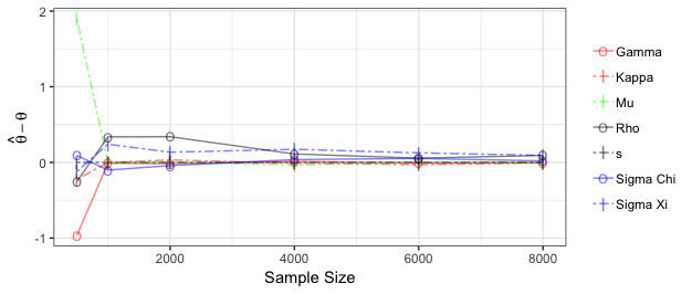
Figure 2: Componentwise estimation error plots for $\theta$ versus $n$.

The convergence of the parameter estimates can be seen in Figure 2, where the estimation errors $\hat{\theta}_{i}-\theta_{i},i=1,2,...,7$ are plotted versus the sample size $n$, $\theta$ is the vector of true parameter values.

The paths of the estimated state variables ${\hat{\chi}}$ and ${\hat{\xi}}$ were obtained through Kalman Filter along with the simulated trajectories of $\chi$ and $\xi$ and their 95%-Confidence Intervals (CIs) based on the true values of the model parameters are presented in Figure 3.

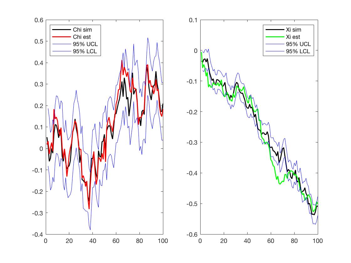
Figure 3: Estimated $(n=8000),{\hat{\chi}}_{t}$, ${\hat{\xi}}_{t}$ and simulated $\chi_{t}$, $\xi_{t}$ paths with their 95% CI.

The plots of the paths of the estimated $\hat{S}_{t}=\exp(\hat{\chi}_{t}+\hat{\xi}_{t})$ and the spot prices $S_{t}=\exp(\chi_{t}+\xi_{t})$ computed using the simulated paths of ${\chi}$ and ${\xi}$ along with 95% CI based on the true model parameter values $\theta$ are presented in Figure 4.

In the AWS Australian Sydney computing center, for computations in Matlab we used c5.18xlarge instances (CPU 36) taking 10 hours for $n=8000$.

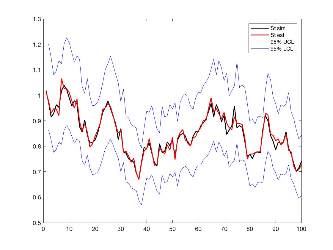
Figure 4: Estimated $\hat{S}_{t}$ and simulated $S_{t}$ with its 95% CI.

5 Conclusions

In this paper, the parameter estimation problem has been studied in the linear partially observable system, which is specific for commodity futures prices developed in the Schwartz-Smith’s two-factor model in the risk-neutral setting. In the simulation study, the Kalman Filter algorithm has been implemented and tested for estimation of the parameters of the bivariate O-U process $x$ jointly with the estimation of its unobserved components $\chi$ and $\xi$. In this study, we suggested the remedy for rectifying the parameter identification problem arising within MLE procedure in the Kalman Filter. The simulation study illustrated the robustness of the grid-search and consistency of the estimates of the model parameters and state vector $x$.

Appendix 0.A Derivations of (1) and (2)

In Section 2.1, we define an Ornstein-Uhlenbeck process as

$$d\chi_{t}=-\kappa\chi_{t}dt+\sigma_{\chi}dZ_{t}^{\chi}$$ (8)

and a mean reverting process

$$d\xi_{t}=(\mu_{\xi}-\gamma\xi_{t})dt+\sigma_{\xi}dZ_{t}^{\xi},$$ (9)

where $dZ_{t}^{\chi},dZ_{t}^{\xi}\sim N(0,\sqrt{\Delta t})$ are correlated standard Brownian motions. Here we provide details to get equation (1) amd (2) from (8) and (9). Firstly, from (8),

$$\Delta\chi_{t}=-\kappa\chi_{t}\Delta t+\sigma_{\chi}\sqrt{\Delta t}\epsilon_{\chi}.$$

Therefore,

$$\chi_{t+1}=(1-\kappa\Delta t)\chi_{t}+\sigma_{\chi}\sqrt{\Delta t}\epsilon_{\chi}.$$ (10)

Similarly, from (9), we get

$$\xi_{t+1}=(1-\gamma\Delta t)\xi_{t}+\mu_{\xi}\Delta t+\sigma_{\xi}\sqrt{\Delta t}\epsilon_{\xi},$$ (11)

where $\epsilon_{\chi},\epsilon_{\xi}\sim N(0,1)$. Let $Corr(\epsilon_{\chi},\epsilon_{\xi})=\rho$ and $w=\left(\begin{matrix}\sigma_{\chi}\sqrt{\Delta t}\epsilon_{\chi}\\ \sigma_{\xi}\sqrt{\Delta t}\epsilon_{\xi}\end{matrix}\right)$, then

$$W=Var(w)=\left(\begin{matrix}\sigma_{\chi}^{2}\Delta t&\rho\sigma_{\chi}\sigma_{\xi}\Delta t\\ \rho\sigma_{\chi}\sigma_{\xi}\Delta t&\sigma_{\xi}^{2}\Delta t\end{matrix}\right).$$ (12)

Let $X_{t}=\left(\begin{matrix}\chi_{t}\\ \xi_{t}\end{matrix}\right)$, $c=\left(\begin{matrix}0\\ \mu_{\xi}\Delta t\end{matrix}\right)$ and $G=\left(\begin{matrix}1-\kappa\Delta t&0\\ 0&1-\gamma\Delta t\end{matrix}\right)$. Then from (10) and (11) we get

$$X_{t+1}=c+GX_{t}+w_{t+1}.$$

Let $\phi=1-\kappa\Delta t$, $\psi=1-\gamma\Delta t$. Then

$$E(X_{t})=\left(\begin{matrix}(1-\kappa\Delta t)\chi_{t-1}\\ (1-\gamma\Delta t)\xi_{t-1}+\mu_{\xi}\Delta t\end{matrix}\right)$$

$$=\left(\begin{matrix}(1-\kappa\Delta t)^{n}\chi_{0}\\ (1-\gamma\Delta t)^{n}\xi_{0}+(1-\gamma\Delta t)^{n-1}\mu_{\xi}\Delta t+...+(1-\gamma\Delta t)^{0}\mu_{\xi}\Delta t\end{matrix}\right)$$

$$=\left(\begin{matrix}\phi^{n}\chi_{0}\\ \psi^{n}\xi_{0}+\mu_{\xi}\Delta t\frac{1-(1-\gamma\Delta t)^{n}}{\gamma\Delta t}\end{matrix}\right)$$

$$=\left(\begin{matrix}\phi^{n}\chi_{0}\\ \psi^{n}\xi_{0}+\frac{\mu_{\xi}}{\gamma}(1-\psi^{n})\end{matrix}\right),$$ (13)

and

$$Var(X_{t})=G\cdot Var(X_{t-1})\cdot G^{\prime}+W=G^{n}Var(X_{0})(G^{\prime})^{n}+G^{n-1}W(G^{\prime})^{n-1}+...+G^{0}W(G^{\prime})^{0}.$$

If we assume $Var(X_{0})=0$, we can get

$$Var(X_{t})=G^{n-1}W(G^{\prime})^{n-1}+...+G^{0}W(G^{\prime})^{0}$$

$$=\left(\begin{matrix}\sigma_{\chi}^{2}\Delta t\sum_{i=0}^{n-1}\phi^{2i}&\rho\sigma_{\chi}\sigma_{\xi}\Delta t\sum_{i=0}^{n-1}(\phi\psi)^{i}\\ \rho\sigma_{\chi}\sigma_{\xi}\Delta t\sum_{i=0}^{n-1}(\phi\psi)^{i}&\sigma_{\xi}^{2}\Delta t\sum_{i=0}^{n-1}\psi^{2i}\end{matrix}\right)$$

$$=\left(\begin{matrix}\sigma_{\chi}^{2}\Delta t\frac{1-\phi^{2n}}{1-\phi^{2}}&\rho\sigma_{\chi}\sigma_{\xi}\Delta t\frac{1-(\phi\psi)^{n}}{1-\phi\psi}\\ \rho\sigma_{\chi}\sigma_{\xi}\Delta t\frac{1-(\phi\psi)^{n}}{1-\phi\psi}&\sigma_{\xi}^{2}\Delta t\frac{1-\psi^{2n}}{1-\psi^{2}}\end{matrix}\right).$$ (14)

When $n\to\infty$, $\Delta t=t/n\to 0$, $\Delta t^{2}=0$, then

$$\phi^{n}=(1-\frac{\kappa t}{n})^{n}\to e^{-\kappa t},$$

$$\psi^{n}=(1-\frac{\gamma t}{n})^{n}\to e^{-\gamma t},$$

$$(\phi\psi)^{n}=(1-(\kappa+\gamma)t/n)^{n}\to e^{-(\kappa+\gamma)t},$$

$$1-\phi^{2}=2\kappa\Delta t,1-\psi^{2}=2\gamma\Delta t,1-\phi\psi=(\kappa+\gamma)\Delta t.$$

From equation (13) and (14), we have

$$E(X_{t})=\left(\begin{matrix}e^{-\kappa t}\chi_{0}\\ e^{-\gamma t}\xi_{0}+\frac{\mu_{\xi}}{\gamma}(1-e^{-\gamma t})\end{matrix}\right)$$

and

$$Var(X_{t})=\left(\begin{matrix}\frac{\sigma_{\chi}^{2}}{2\kappa}(1-e^{-2\kappa t})&\frac{\rho\sigma_{\chi}\sigma_{\xi}}{\kappa+\gamma}(1-e^{-(\kappa+\gamma)t})\\ \frac{\rho\sigma_{\chi}\sigma_{\xi}}{\kappa+\gamma}(1-e^{-(\kappa+\gamma)t})&\frac{\sigma_{\xi}^{2}}{2\gamma}(1-e^{-2\gamma t})\end{matrix}\right),$$

in the linearised form $Var(X_{{\Delta}t})\approx W$ from (12).

References

• [1] Ames, M., Bagnarosa, G., Matsui, T., Peters, G., Shevchenko, P.V.: Which risk factors drive oil futures price curves? Available at SSRN 2840730 (2016)
• [2] Binkowski, K., Shevchenko, P., Kordzakhia, N.: Modelling of commodity prices (2009), CSIRO technical report
• [3] Black, F.: The pricing of commodity contracts. Journal of Financial Economics 3, 167–179 (1976)
• [4] Cheng, B., Nikitopoulos, C.S., Schlögl, E.: Pricing of long-dated commodity derivatives: Do stochastic interest rates matter? Journal of Banking and Finance 95, 148–166 (2018)
• [5] Cortazar, G., Millard, C., Ortega, H., Schwartz, E.S.: Commodity price forecasts, futures prices and pricing models (2016), http://www.nber.org/papers/w22991.pdf
• [6] Ewald, C.O., Zhang, A., Zong, Z.: On the calibration of the Schwartz two-factor model to WTI crude oil options and the extended Kalman filter. Annals of Operations Research pp. 1–12 (2018)
• [7] Favetto, B., Samson, A.: Parameter estimation for a bidimensional partially observed Ornstein–Uhlenbeck process with biological application. Scandinavian Journal of Statistics 37(2), 200–220 (2010)
• [8] Gibson, R., Schwartz, E.S.: Stochastic convenience yield and the pricing of oil contingent claims. Journal of Finance pp. 959–976 (1990)
• [9] Gilbert, P.: Brief user’s guide: Dynamic systems estimation (dse). Available in the file doc/dse-guide. pdf distributed together with the R bundle dse, to be downloaded from http://cran. r-project. org (2005)
• [10] Harvey, A.C.: Forecasting, Structural Time Series Models and the Kalman Filter. Cambridge University Press (1990)
• [11] Helske, J.: Kfas: Exponential family state space models in r. arXiv preprint arXiv:1612.01907 (2016)
• [12] Hull, J.C.: Options, Futures, and Other Derivatives. Prentice Hall, 8th edn. (2012)
• [13] Kutoyants, Y.A.: On parameter estimation of the hidden Ornstein–-Uhlenbeck process. Journal of Multivariate Analysis 169, 248–263 (2019)
• [14] Ornstein, L.S., Uhlenbeck, G.E.: On the theory of the Brownian Motion. Physical Review 36(5) (1930)
• [15] Peters, G., Briers, M., Shevchenko, P., Doucet, A.: Calibration and filtering for multi factor commodity models with seasonality: Incorporating panel data from futures contracts. Methodology and Computing in Applied Probability 15 (2013)
• [16] Schwartz, E., Smith, J.E.: Short-term variations and long-term dynamics in commodity prices. Management Science 46(7), 893–911 (2000)
• [17] Schwartz, E.S.: The stochastic behavior of commodity prices: Implications for valuation and hedging. The Journal of Finance 52(3), 923–973 (1997)
• [18] Shumway, R.H., Stoffer, D.S.: Time series analysis and its applications: with R examples. Springer (2017)
• [19] Tusell, F.: Kalman filtering in R. Journal of Statistical Software 39 (2011)