What’s Wrong with the Bottom-up Methods in Arbitrary-shape Scene Text Detection

Abstract

The latest trend in the bottom-up perspective for arbitrary-shape scene text detection is to reason the links between text segments using Graph Convolutional Network (GCN). Notwithstanding, the performance of the best performing bottom-up method is still inferior to that of the best performing top-down method even with the help of GCN. We argue that this is not mainly caused by the limited feature capturing ability of the text proposal backbone or GCN, but by their failure to make a full use of visual-relational features for suppressing false detection, as well as the sub-optimal route-finding mechanism used for grouping text segments. In this paper, we revitalize the classic text detection frameworks by aggregating the visual-relational features of text with two effective false positive/negative suppression mechanisms. First, dense overlapping text segments depicting the ‘characterness’ and ‘streamline’ of text are generated for further relational reasoning and weakly supervised segment classification. Here, relational graph features are used for suppressing false positives/negatives. Then, to fuse the relational features with visual features, a Location-Aware Transfer (LAT) module is designed to transfer text’s relational features into visual compatible features with a Fuse Decoding (FD) module to enhance the representation of text regions for the second step suppression. Finally, a novel multiple-text-map-aware contour-approximation strategy is developed, instead of the widely-used route-finding process. Experiments conducted on five benchmark datasets, i.e., CTW1500, Total-Text, ICDAR2015, MSRA-TD500, and MLT2017 demonstrate that our method outperforms the state-of-the-art performance when being embedded in a classic text detection framework, which revitalises the superb strength of the bottom-up methods.

I Introduction

DEEP learning based arbitrary-shape scene text detection methods generally follow two streams, i.e., top-down approaches and bottom-up approaches.

The top-down approaches usually consider a text instance as a whole and reason its text area through leveraging the segmentation results, whereas the bottom-up methods try to divide a text instance into text segments and then group them based on certain criteria. Both types of approaches [1, 2, 3, 4, 5, 6, 7, 8, 9] use a feature extraction network [10, 11] with a Feature Pyramid Network (FPN) [12] as the basic text feature extraction network, and are deemed as the classic text detection framework. The major difference is that the goal of the top-down methods is to generate more accurate segmentation masks for text areas. Consequently, more sophisticated modules from the object detection and semantic segmentation field have been adopted to enhance the performance of text segmentation. However, these methods may not be robust for long text instances due to their limited reception field as well as the insufficient geometric feature representation of CNN [13, 3].

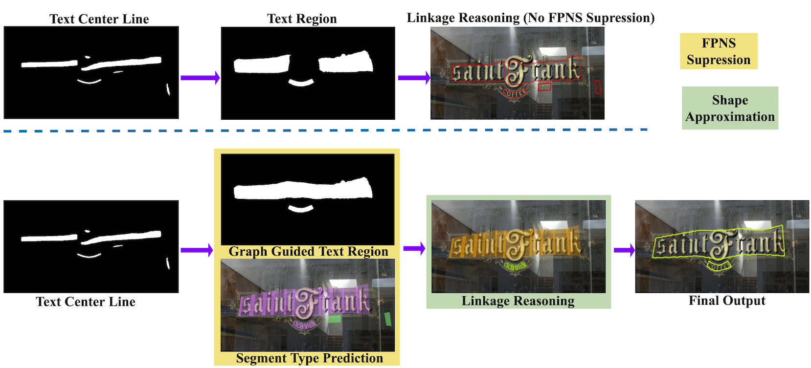
Figure 1: The error accumulation problem of the existing bottom-up approaches (top) and our solution (bottom). Our Graph Guided Text Region fuses relational features with visual features and rectifies false detection. The segment type prediction module further rectifies this through excavating the ‘characterness’ and connectivity of text segments.These two modules are designed for one goal, i.e., suppressing false positive/negative samples in the inference stage. The Final Output shows that the false detection has been suppressed.

The bottom-up methods [14, 3, 4, 7, 2] typically decompose a text instance into several components and then group the eligible ones together with certain purposefully designed rules. Intuitively, these methods align better with the way how humans read text. Besides, the bottom-up methods often require smaller reception fields and are therefore more flexible for modelling arbitrary-shape texts. Therefore, they are expected to yield higher accuracies and better robustness for long and curved texts. However, the reality is often the opposite, since the bottom-up methods are also prone to accumulating intermediate errors (false positives/negatives). For example, in the challenging curved text datasets CTW1500 [15] and Total-Text [16], the overall accuracy of the bottom-up methods is lower than the best performing top-down methods [5, 17, 6, 18]. What is wrong with the bottom-up methods?

To resolve this mystery, we need to analyze the development process of the bottom-up methods in the deep learning era. Due to that the focus of the text detection research has been extended from detecting horizontal text to detecting quadrilateral text, and then to detecting more challenging, curved text, the relationship between text segments has become more diverse and complicated. In order to connect text segments, visual similarity features, sequential features and geometric features have been considered by the existing bottom-up methods [19, 2, 20, 21, 14, 8] with CNN, RNN and some pre-defined heuristic rules.

However, the relationship between text segments is non-Euclidean, which means there may still be connections between non-adjacent text segments especially in the case of curved texts. The Graph Neural Network (GNN) is an effective framework for representing this kind of non-Euclidean data, as it learns the representation of each node by aggregating the features from adjacent nodes [22]. In terms of better capturing the relationship between text segments, the state-of-the-art bottom-up methods such as DRRG [7], ReLaText [3] and PuzzleNet [4] have already adopted GCN [23]. These methods share a similar framework, namely, a text segment proposal network (e.g., VGG16/ResNet50+FPN) followed by a relational reasoning (link prediction) networks (e.g., GCN). Nevertheless, the performance of these bottom-up methods is still lower than that of the top-down methods [5, 17, 24].

There are two problems that need to be addressed. First, the simple connection between the text proposal network and the GCN tends to result in error accumulation. An example is shown in Fig. 1, where the wrongly separated text (false negatives) and two text-like objects (false positives) from the FPN layer of the text segment proposal network have been further propagated after the linkage prediction by GCN. Here, the Text Region/Text Center Line results generated from the same layer of FPN share similar visual features, which are often designed as a double guarantee for accurate text areas and generation of text segments for further relational reasoning. However, sharing similar visual feature sometimes lead to error accumulation. In this example, a text instance appears to be separated in both text region map and its center line map as the FPN layer cannot build long range dependency between the text segments for this text instance. Although the relational information predicted by GCN can be treated as long range dependency for different text segments, the simple connection of FPN and GCN has completely wasted the relational features. Even if the text region and its center line are both considered for generating text segments, some of the text segment candidates will still be wrongly discarded, which significantly affects the accuracy of linkage prediction of GCN. This is the reason why the final detection result (the top-right figure) accumulates wrongly separated situation from text region and its center line. Here, simple connections between FPN and GCN and the weight sharing design in the FPN layer cannot solve the problem of false detection. Thus, the reasoning of text region needs stronger relational cues to ensure their connectivity and integrity.

Also, simple connection causes the text segments in false positives to be treated by GCN indiscriminately the same as other text segments in the subsequent linkage reasoning steps, leading to that two text-like objects are falsely detected after linkage prediction of text segments. Among the GCN based bottom-up approaches, only ReLaText has attempted to randomly generate some non-text nodes to GCN and remove the link between two non-text nodes. But this step is insufficient to the false positives/negatives suppression (FPNS), nor does it make a full use of the relational information.

Since the spaces between texts or characters are also non-text areas, GCN may not be able to distinguish text gaps from the non-text background, nor does the text segment proposal network. As shown in the separated text instance in Fig. 1 (better viewed in darker colors), the separated area is right in the interval area of the text. As pointed out by [25], lacking content information increases the possibility of false detection, indicating that too large [4] or too sparse text segments [3, 7] cannot reflect the ‘charactarness’ of the content information of texts.

The other problem occurs in the text segments’ final grouping stage. This stage is also known as the inference stage [2, 7, 20, 19], but is often underestimated with relatively fewer descriptions and has a major impact on the results. Its goal is to locate all the points on the contour and specify the correct visiting order through these points [7]. It should be noted that the directional search towards the ends of text instances in TextSnake [20], the sorting of the text segments’ bounding boxes in TextDragon [26], the searching of the polynomial curve that fits two long sides of text instances in ReLaText, and the segmentation of the bisection lines based on the vertex extraction in PuzzleNet are all different forms of searching the visiting order of contour points. This is analogous to the Traveling Salesman problem, which is an NP-complete problem. The DRRG [7] used a greedy Min-Path algorithm to give an approximate solution to this problem. However, approximating solutions can sometimes fall into the local optimal situations (see Fig. 2(a)) when there are too many contour points. PuzzleNet [4] and ReLaText [3] adopted larger text segments to control the number of contour points, while large text segments can weaken the character level information and also compromise the flexibility when grouping segments into text instances. How to find the text contour without diminishing the ‘charactarness’ of texts and without introducing sub-optimal failures needs to be further explored.

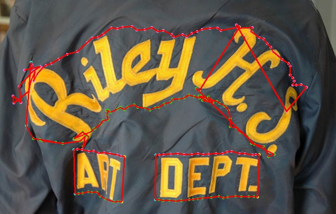
(a) Route-finding failure from [7]

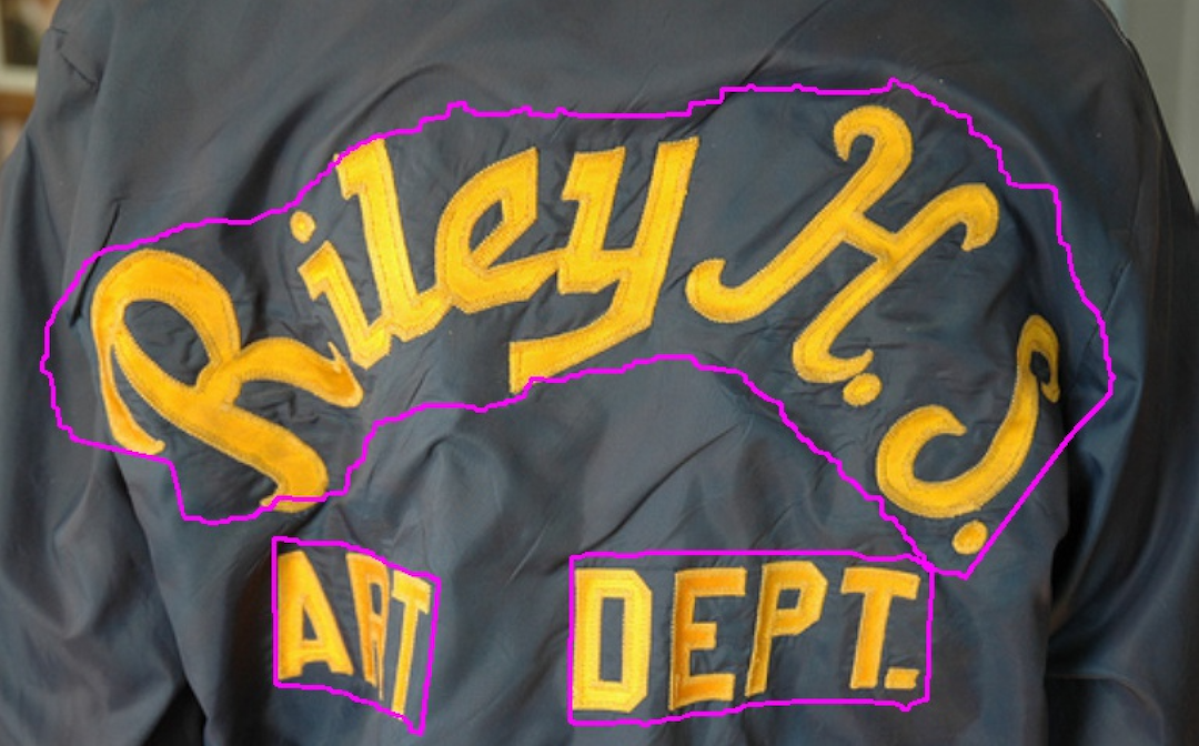
(b) Our shape-approximation solution

Figure 2: Route-finding gives sub-optimal visiting order when there are too many contour points. The crossing lines are caused by wrong visiting order of intermediate points.

To address the above issues, we develop a strategy that aggregates visual and relational text feature maps to suppress the false detection, including both false positives and false negatives. This is shown in Fig. 1. Instead of considering only visual text feature maps from the output of FPN layers, here we propose a Location-Aware Transfer (LAT) to convert relational features produced by GCN to become visual compatible features. Then, a Fuse Decoding (FD) module is introduced to fuse the relational features with the visual features for generating Graph Guided Text Region (GGTR) map, which can be seen as additional long range dependency to guide connectivity and integrity of text region. The GGTR map can now be used as alternative guarantee for FPNS and the generation of enough candidate text segments for further graph reasoning.

In the text proposal step, the rectangular text segments are designed in a dense and partially overlapping manner so as to retain their ‘streamline’, which allows flexible connection as much as possible. The dense overlapping text segments will also guarantee connectivity when combined with the link prediction from GCN. To make sure that the text segments are able to depict the ‘charactarness’ of text, the text segment are designed to be fine enough to reflect character and text spacings (see the segment type prediction in Fig. 1). We also build a weakly supervised GCN to further classify the types of text segments based on their link prediction results. This establishes a backward feedback mechanism that can retrieve and suppress false detection on the text maps from the text proposal layer. Classifying the types of segments enables the GCN to learn the content information for more accurate text region prediction.

Furthermore, in the inference stage, we decompose the overall text map rectification problem into the problem of rectifying text segments so as to improve their fault tolerance ability. Instead of the route-finding process, we group the overlapping text segments to approximate the contour of the original text instance by integrating the aggregated information with both visual reasoning and relational reasoning for more accurate text contour finding.

In summary, the main contributions of our work are:

1) We propose a novel visual-relational reasoning approach to revitalize the superb strength of the bottom-up text-detection approaches on a redesigned dense, overlapping text segments modelling the ‘characterness’ of text. This is demonstrated to be more effective in capturing both visual and continuous property of the characters that determines text areas.

2) We propose a simple but effective contour inference module specially designed for the bottom-up approaches that replaces the traditional route-finding process by approximating the contour of the grouped text segments. This module can address complex situations that involve a large number of text segments.

3) Our approach revitalizes the superb strength of the existing bottom-up methods and surpasses the state-of-the-art performance on several curved text detection benchmark datasets using only VGG16+FPN backbone and single-scale training and testing. This further proves that the bottom-up methods are not inferior to, but can be even better than, the top-down methods in arbitrary-shaped text detection.

II Related Work

II-A Bottom-up Text Detection Methods

CTPN [19] is a pioneer work that brings text detection into the deep-learning area, but it simply merges text segments according to a certain threshold and can only deal with horizontal texts. SegLink [14] is designed to detect multi-oriented texts, which aims to connect the centers of two segments with an eight-neighbourhood link prediction. Subsequently, as the research focus has changed to curved text, text detection has transitioned from the detection of bounding boxes to the detection of contours. TextSnake [20] is the first work to attempt this transition by using several circles with predictable angles and radius to fit curved texts. At this point, both geometric and visual information has been largely considered in curved text detection.

To further excavate the relationship between text segments, Baek et al. [2] used affinity boxes to describe the neighbouring relation between text segments for further spatial reasoning, but it was insufficient for reasoning the complex relationship between curved texts and reflecting the ‘charactarness’ of texts. Later, researchers used GCN to integrate geometric features, visual features, and relational features for link prediction [7, 3, 4]. These three methods share a similar framework but differ in the size and number of text segments. PuzzleNet [4] used the largest text segments to merge adjacent text segments with angle differences less than $\pi/36$, which was very inflexible in the following segments grouping stage. RelaText [3] generated smaller text segments compared with PuzzleNet, but they were still too large and too sparse to depict the character features of the text. The size of the text segments in DRRG [7] is the smallest, and although it contains more char-level features and is more flexible when grouping, the complexity of its route-finding process increases significantly. Thus, there is often a trade-off between the size and number of text segments and the difficulty of the grouping operation, which needs to be further explored.

In our approach, we use ‘characterness’ and ‘streamline’ to accurately depict the character-level and adjacency-level features of text content, which avoids the computational overload of the route-finding process with a shape approximation (SAp) strategy while greatly increasing flexibility.

II-B False Detection Suppression

Suppressing false detection requires distinguishing text and non-text areas accurately. The first way is to strengthen the network’s capability for depicting text features by adding additional text content information. Some methods try to use char-level annotation to increase the ‘characterness’ expression. For example, CRAFT [2] adopted a weakly-supervised training strategy to train the character region score to split words into characters; TextFuseNet [5] fused word-level, char-level and global-level features of text to conduct text instance segmentation using Mask-RCNN [27]. Similarly, Zhang et al. [28] also used this framework to obtain char-level annotation with a weakly-supervised training strategy. However, training char-level annotation as an instance segmentation task means doing detection and recognition together, which brings additional computational burden. Other methods such as [4, 28, 29, 3, 30, 17, 31, 32] try to insert blocks like Non-local [33] or Deformable Convolution [34] to increase the network’s capability for extracting text features, but these tricks are really a bit ‘icing on the cake’ if we look at their detection results. We need to focus more on the characteristic of the text itself.

The other way is to jointly consider multiple text maps to get a final text area. ContourNet [6] tried to suppress non-text areas by considering text maps in horizontal and vertical directions, which effectively suppressed false positives. Nevertheless, their method still suffers from the false negatives when both horizontal and vertical text maps have defects. TextSnake [20] and DRRG [7] predicted an additional Text Center Line (TCL) map and multiplied it with the original Text Region (TR) map to the FPNS. As shown in Fig. 1, both TCL and TR are resulted from FPN. It is very likely that both TCL and TR maps are flawed, which may result into the error accumulation problem.

Moreover, simply setting a threshold on different text maps [6] or directly multiplying different text maps globally increases the risk of having the true positive text areas suppressed as well. It needs to have a more effective and accurate approach to each text instance on text maps and indirectly use both of them.

III Methodology

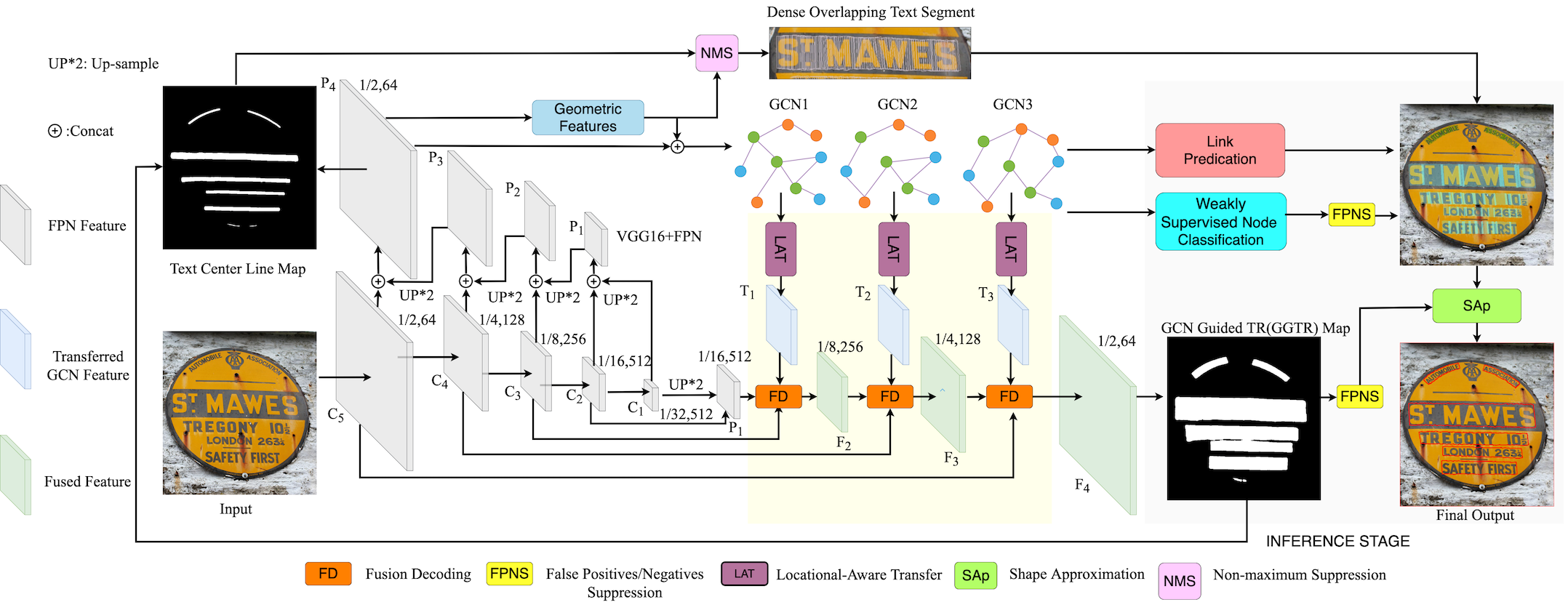
Figure 3: The overall structure of our network. The “1/2,64”, “1/4,128”,… and “1/16,512” indicate the scale ratio and the channel number of the input image.

The overall structure of our network is illustrated in Fig. 3, where the commonly used VGG16 with an FPN is used to generate Text Center Line (TCL) maps as well as geometric features for dense, overlapping rectangular text segments.

In this figure, $C_{5}$ to $C_{1}$ represent the feature maps after pooling from VGG16, $P_{1}$ to $P_{4}$ stand for the up-sampled features at each layer from the FPN, $T_{1}$ to $T_{3}$ stand for the transferred GCN features by Location-Aware Graph Feature Transfer module, and $F_{1}$ to $F_{3}$ are the fused features of the transferred GCN features and FPN features by our proposed graph feature Fusion Decoding module (FD), which are used to generate a Graph Guided Text Region (GGTR) map to further refine the detection results.

Meanwhile, we also explore the strategy of weakly supervised learning to classify each text segment into one of the three types, i.e., char segments, interval segments and non-text segments. Then, we feed the text segments and their type information into GCN as nodes to train the network to learn the link relationship and node types. Multiple text maps as well as link relationship and segment types are further combined during the inference stage. Finally, a novel text-instance based contour inference module is used to approximate the contour of the connected text segments to obtain the final results.

III-A Dense Overlapping Text Segments

The goal of dense overlapping text segments is to depict the character-level and adjacency-level features of text content, as well as provide training label for the graph reasoning step. In this section, we first introduce geometric feature prediction of text segments. Following that, the annotation of each text segment according to the content information of texts is presented.

III-A1 Text Segments Generation

In our work, we first adopt the commonly used VGG16+FPN for generating the TCL map, as well as the geometric features for each text segment. The text segments are defined by $(x,y,h,w,\theta)$ as small rectangles, where $x$ and $y$ represent the $X$ and $Y$ coordinates of the rectangle’s center point, and $h$, $w$ and $\theta$ represent the height, width and the rotation angle of the rectangle, respectively.

As shown in Fig. 3, the final extracted features $P_{4}$ are used to generate the TCL map, and the geometric features (i.e., Height map $H$ and Angle map $\Theta$) to restore the geometric representation of text segments.

More specifically, $Conv_{1\times 1}$ is applied on $P_{4}$ to obtain these text maps, namely, TCL, H and $\Theta$. In our work, the Width map (W) is obtained by applying a clip function to the Height map while keeping the width between 2-6 pixels, as shown in Fig. 4. Sect. IV-D further discusses the impact of the width value on the final results.

Note that, our constructed visual representation for each text segment is designed to depict the ‘characterness’ and ‘streamline’ of the text instance, as characters in a text instance are usually slender, and therefore text segments with a smaller width can increase the accuracy for using their connected shape to approximate the actual text instance. Also, smaller text segments may better differentiate chars, char spacing and word spacing in the text, which will be used to further suppress false detection. The ablation studies conducted in Sect. IV-D demonstrate this.

Moreover, the ground truth of the TCL map is adopted by shrinking the ground truth of the text area using the method described in [7, 20], which reduces the length of $h$ in the text segments. To generate dense overlapping text segments, here we first generate small rectangles for each pixel in the text areas of the TCL map with geometric features from the Height, Width and Angle map. It should be noted that in the inference stage, the TCL map will be rectified by the GGTR map before generating dense overlapping text segments. Then, the NMS algorithm with an IoU threshold of 0.5 is applied on this TCL map to remove duplicated rectangles. As discussed later, this step ensures the density and connectivity of the text segments, which will increase the flexibility for them to adapt to various arbitrary shapes.

III-A2 Annotation of Text Segments

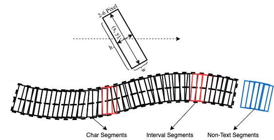
Figure 4: The three types of the text segments.

After we have obtained the dense overlapping text segments, the next step is to determine their types, which are used for training GCN to classify the type of text segments. The text segments are categorized into one of the three types, namely, char segments, interval segments and non-text segments (as shown in Fig. 4), for depicting the ‘characterness’ of text.

The interval segments are the gaps or spacing between the characters or words, which are often confused with non-text segments for some text instances with larger inter-character spaces. Thus, we take into consideration their context segments to enable GCN to have the ability to classify these text segments correctly for further FPNS. Therefore, we need the type annotation of the segments. Although there is no dataset that can provide annotation for the intervals between characters, this annotation can be obtained by utilizing the synthetic dataset [35] that has character level annotation. We use the character maps and their interval spaces to annotating char segments and interval segments.

Here, we use $S^{i}$ to denote the $i$-th text segment that needs to be annotated and $(x_{i},y_{i})$ is the coordinate of the center point of this segment. $S^{*}$ represents the collection of all text segments, while $S_{char}^{*}$ and $S_{\neg char}^{*}$ are used to denote the collection of the char segments and non-char segments. $C$ is used to denote the union of all character maps in the image. $S_{char}^{*}$ are the text segments whose center $(x,y)$ locates in the union of char areas in $C$. The non-char segments $S_{\neg char}^{*}$ can be obtained by $S^{*}-S_{char}^{*}$.

Then, we define the distance between each text segment in $S_{char}^{*}$ and non-text segment in $S_{\neg char}^{*}$ as the Euclidean distance between the center points of two segments as:

$$d(S_{char}^{i},S_{\neg char}^{j})=\left\|(x_{i},y_{i})-(x_{j},y_{j})\right\|_{2},$$ (1)

where $\forall S_{char}^{i}\in S_{char}^{*}$ and $\forall S_{\neg char}^{j}\in S_{\neg char}^{*}$.

This step is used to find out the interval segments in the non-char segments. It should be noted that not all non-char segments are considered as interval segments for datasets that come with word-level annotations. This is because the following weakly supervised training strategy in our work may lead to some char segments being mistakenly labeled as interval segments. Therefore, to increase the robustness of interval segment selection, for each char segment $S_{char}^{i}$, there is one closest interval segment $S_{inter}^{i}$, which is the non-char segment that has the minimal Euclidean distance from $S_{char}^{i}$, i.e.,

$$\!S_{inter}^{i}\!\!=\!\left\{{S_{\neg char}^{k}\big{|}d(S_{char}^{i},S_{\neg char}^{k})\!=\!\!\!\!\!\!\!\min_{\!j\leq|S_{\neg char}^{*}|\!}\!\!\!\!d(S_{char}^{i},S_{\neg char}^{j})\!}\right\}.$$ (2)

Here, we use $S_{inter}^{*}$ to denote the collection of all interval segments. Although the closest non-char segments are considered as the interval segments, the final results show that some non-char segments near the char segments can still be correctly classified as interval segments after weakly supervised training (see the interval segments in Figs. 1 and 5).

Finally, the non-text segments $S_{\neg text}^{*}$ are generated based on the inverse of the ground truth of text region. Several center points $(x,y)$ are randomly picked from the non-text area of the ground truth of text region. Other geometric features of text segments $(h,w,\theta)$ are selected randomly from $S_{inter}^{*}$ and $S_{char}^{*}$.

Once the char segments, interval segments and non-text segments are annotated, we can train the GCN layer to classify the type of text segments. The datasets without char-level annotations are trained with a weakly supervised strategy, where we first use a model pre-trained on the synthetic dataset [35] to predict the coarse types of text segments. Since our goal is the FPNS, we mainly consider the correctness of distinguishing non-text segments and interval segments to filter poor annotation results. Here, the ground truth of text regions is used to guide the training, avoiding confusing non-text segments with interval segments and char segments. With such an iterative approach, we can pick out the cases where the annotation results are correct and add them to the annotation of the training set. See Fig. 5 for examples of the text segment annotation results after weakly supervised training.

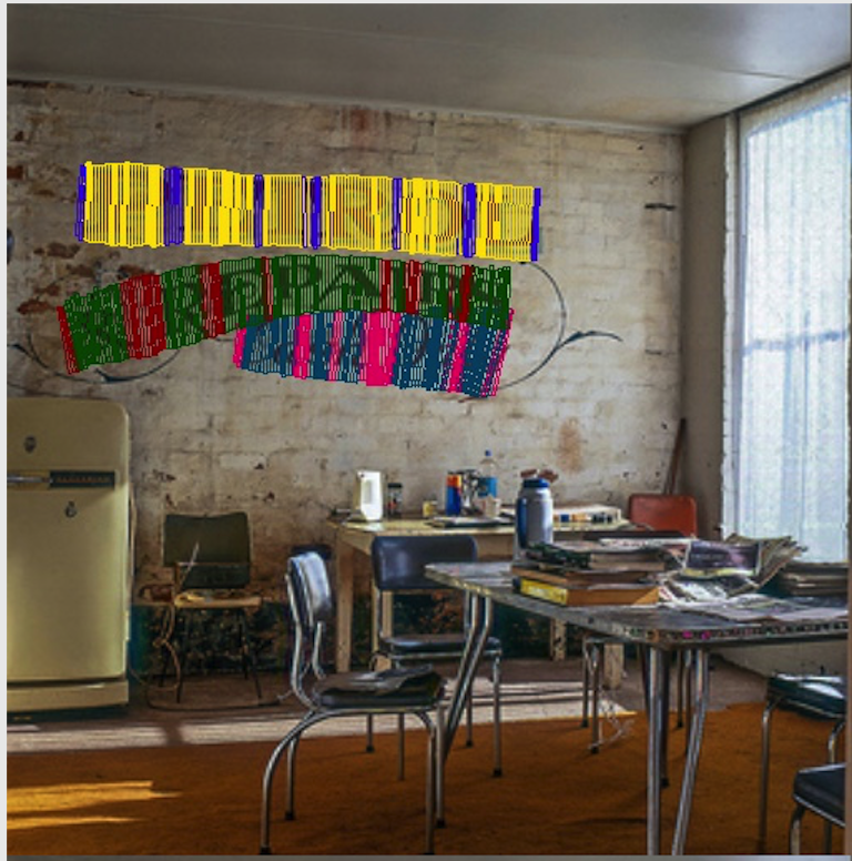
Figure 5: The results of weakly supervised training step (1st row) and the original images overlaid with ground truth (2nd row). The interval segments and char segments are shown with different colors. The GCN now has the ability to classify the type of segments, which will benefit the following FPNS step. Note that, in these figures, non-text segments are not displayed for a cleaner look.

III-B Graph based Reasoning and Fusion

After we obtain dense overlapping text segments and their annotations, GCN is used to explore the relational representation between text segments. This representation will be directly involved in our fusion decoding module and FPNS strategy.

III-B1 Link Prediction and Classification

To predict the links between text segments and classify the type of each text segment, we first need to integrate the feature representation of each text segment and construct the graph structure of them.

Here, we consider two kinds of features for text segments, i.e., the visual feature $F_{vis}$ from $P_{4}$ in FPN and the geometric feature $F_{geo}$ of the text segments. We use $F_{seg}$ for the relational feature representation matrix of text segments. Following the methods in [4, 7], the RRoI Align [36] is adopted to pool the visual feature from FPN. $F_{geo}$ is calculated from feature maps TCL, H, W and $\Theta$, and is embedded into the same space as $F_{vis}$ as:

$$F_{seg}=[F_{vis}(P_{4});F_{geo}([TCL;H;W;\Theta])],$$ (3)

where the $[;]$ operator means concatenation.

To build the graph structure of text segments, we treat each text segment as the pivot and connect its eight closest text segments as its 1-hop nodes. Then, for each 1-hop node, we connect its four closest text segments (excluding the pivot). Here, the distance between two text segments is measured by the Euclidean distance of their center points. The pivot, 1-hop nodes and 2-hop nodes compose the basic graph structure for every text segment, which can be represented by an adjacency matrix $\mathcal{A}$. We consider the top three closest text segments of a pivot that should have a link with the pivot. Similar to those in [37, 23, 7], the graph convolution is represented by:

$$F_{seg}^{(i+1)}=\sigma([F_{seg}^{(i)};\tilde{\mathcal{D}}^{\frac{1}{2}}\tilde{\mathcal{A}}\tilde{\mathcal{D}}^{\frac{1}{2}}F_{seg}^{(i)}]W^{(i)}),$$ (4)

where the $F_{seg}^{(i+1)}$ is the feature representation for the $i+1$ layer after the graph convolution of $F_{seg}^{(i)}$. $\tilde{\mathcal{D}}^{\frac{1}{2}}\tilde{\mathcal{A}}\tilde{\mathcal{D}}^{\frac{1}{2}}$ is the re-normalization trick from the original GCN paper [23] and can be calculated by $\mathcal{A}$. $\sigma$ is a non-linear activation function and $W^{(i)}$ is the weight of graph convolutional layer.

Thus, the relational link prediction can be written as:

$$\hat{r}=Softmax(m^{(i+1)}(F_{seg}^{(i+1)})),$$ (5)

where $m^{(i+1)}$ denotes a multi-layer perceptron with a PReLU activation. The feature matrix $F_{seg}$ can also be written as $F_{seg}=[f_{1},f_{2},...f_{v},...]^{T}$, where $f_{v}$ is the feature representation vector for the single text segment $v$.

The GCN segment classification results for the text segment $v$ can be represented by:

$$\hat{f_{v}}=Softmax(\varphi(\frac{1}{|\mathcal{N}(v)|}\sum_{u\in\mathcal{N}(v)}\mathcal{W}f_{u}+b)),\forall v\in\mathcal{V},$$ (6)

where $\mathcal{N}(v)$ means the neighbor segments in the graph structure $\mathcal{V}$ of text segment $v$, and $\mathcal{W}$ and $b$ are the weights of the graph convolution. $\varphi$ is the non-linear activation function. Eq. (6) is the node-level graph feature aggregation of Eq. (4).

After the feature aggregation by GCN, the relational reasoning results can be used to combine text segments that have a strong relationship. The weakly supervised node classification results are used to refine the detection results inherited from the previous FPN layer. Thus, the graph reasoning prevents detection error from being further accumulated. Both link prediction and node classification are required to make inferences based on the visual and relational features of text segments, and can benefit each other when sharing the same weights.

III-B2 Multi-modal Graph Feature Fusion Decoding

Input: $F_{seg}^{i}$, $F_{geo}$

Output: Transferred feature $T_{i}$

$T_{i}=ZeroLike(H,W,C)$

$N=F_{seg}^{i}.shape[0]$

for  $k\leq N$  do

       $(x_{k},y_{k},h_{k},w_{k},\theta_{k})=Geometric(F_{geo},S^{k})$

       if $type(S^{k})\neq nontext$ then

             for $\forall x,y\in bbox(x_{k},y_{k},h_{k},w_{k},\theta_{k})$ do

                   $T_{i}[x,y,:]=F_{seg}^{i}[k,:,:].flatten()$

                  

             end for

            $T_{i}=T_{i}.transpose(2,0,1)$

       end if

      

end for

return $T_{i}$

Algorithm 1 Location-Aware Transfer

We then fuse the relational features with the visual features to complement the long range dependency between text segments for generating graph guided text regions. However, the dimensionality of the relational feature is different from that of the visual feature, which means they cannot be fused directly.

To fuse this relational feature with the visual feature from the normal convolutional layer, we propose Location-Aware Graph Feature Transfer (LAT) to reconstruct the graph convolutional feature of $i$-th GCN layer $F_{seg}^{i}$ in Eq. (4) with consideration of the location information of each node in the graph. The relational features after GCN contain the structural information of the graph in its first two dimensions. For example, the relational feature $F_{seg}^{i}\in\mathbb{R}^{N\times M\times D}$, where $N$ is the total number of nodes (i.e., text segments) in the input image, $M$ is the number of 1-hop nodes, and $D$ is the dimension of GCN feature which is similar to the channel space in the convolutional layer. Our goal is to reshape the $F_{seg}^{i}$ of ${N\times M\times D}$ dimension to ${C\times H\times W}$, where $C$, $W$ and $H$ are the channel, width and height of the input image. The core idea is to fill in the graph features in the corresponding region in the transferred map based on the location information of each text segment. Namely, building connection of the nodes on the graph structure with their location on the image, as the location of each node is also translation invariant compared to the visual feature.

The transferred feature $T_{i}\in\mathbb{R}^{C\times H\times W}$ for $F_{seg}^{i}$ after LAT can be calculated with Algorithm 1.

First, we calculate the geometric feature $(x_{k},y_{k},h_{k},w_{k},\theta_{k})$ of text segment $S^{k}$ by the geometric feature map $F_{geo}$. Here, we only consider transferring the graph features of char/interval segments. Then, we can find the bounding box (bbox) of each text segment on the feature map of $T_{i}$ according to the $(x_{k},y_{k},h_{k},w_{k},\theta_{k})$. For each point ($x,y$) in the bbox, we fill the flattened graph feature into $T_{i}$.

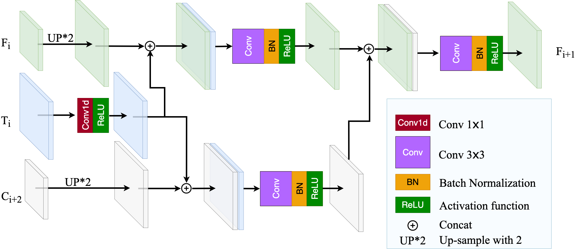
Figure 6: The network structure of multi-modal fusion decoding module.

Since FPN is unable to reason the relationship between different text segments, we introduce a multi-modal Fusion Decoding (FD) module to capture the long range dependency between individual text regions according to their relational features as well as FPN features. The final goal is to generate a graph feature guided text region map for further FPNS. As shown in Fig. 6, the proposed FD module produces the final fused feature $F_{i+1}$ as:

$$F^{\prime}=\left\{\begin{aligned} \mathcal{CBR}[\mathcal{UP}(P_{i});\mathcal{CR}(T_{i})]\quad{\text{if}}\quad i=1\\ \mathcal{CBR}[\mathcal{UP}(F_{i});\mathcal{CR}(T_{i})]\quad\quad\quad\quad\quad\\ \end{aligned}\right.$$ (7)

$$F_{i+1}=\mathcal{CBR}[F^{\prime};\mathcal{CBR}[\mathcal{UP}(C_{i+2});\mathcal{CR}(T_{i})]],$$ (8)

where $\mathcal{CBR}$ denotes $Conv_{3\times 3}$, Batch Normalization and ReLU, $CR$ donates $Conv_{1\times 1}$ and ReLU, and $\mathcal{UP}$ denotes two times of up-sampling.

Finally, we apply the $Conv_{1\times 1}$ on $F_{3}$ to obtain a Graph Guided Text Region (GGTR) map, which will be used as a visual-relational guiding in the inference stage.

III-C Loss Function

The overall objective function consists of six parts and is formulated as:

$$L=L_{GGTR}+L_{TCL}+L_{H}+L_{\theta}+L_{Link}+L_{Node},$$ (9)

where $L_{GGTR}$ and $L_{TCL}$ are the losses from the GGTR and TCL maps, respectively, and $L_{H}$ and $L_{\theta}$ are Smoothed $L1$ losses for Height and Angle. In our work, OHEM [38] is adopted for training the $L_{TCL}$, and the ratio of positive sample and negative sample areas is set to $1:3$.

The linkage loss $L_{Link}$ is computed from the above relational link prediction by:

$$L_{Link}=-r\log\hat{r}-(1-r)\log(1-\hat{r}),$$ (10)

where $r$ is the ground truth of the linkage relationship between text segments and $\hat{r}$ is calculated according to Eq. (5).

For the text segment classification loss $L_{Node}$, since our annotation is obtained with weakly supervised training, we only consider the text segments that are labeled as char segments, interval segments and non-text segments (denoted as $f^{v}_{c}$, $f^{v}_{i}$, and $f^{v}_{n}$ respectively) and ignore those that have not been labeled. Thus,

$$L_{Node}=-(\sum_{v\in\mathcal{N}}{f^{v}_{c}\log{\hat{f^{v}_{c}}}}+\sum_{v\in\mathcal{M}}{f^{v}_{i}\log{\hat{f^{v}_{i}}}}+\sum_{v\in\mathcal{O}}{f^{v}_{n}\log{\hat{f^{v}_{n}}}}),$$ (11)

where $\mathcal{N}$, $\mathcal{M}$, and $\mathcal{O}$ are the collections of all char segments, interval segments and non-text segments, respectively.

III-D Inference by FPNS and Shape-Approximation

The Graph Guided Text Region map and the text segment classification results from the GCN are then used to rectify the TCL map for removing false detection. The relationship prediction and the dense overlapping text segments together ensure the completeness and accuracy of using the contour of the grouped text segments to approximate the contour of text. The connection of the text areas is ensured by the ‘characterness’ and ‘streamline’ of our dense overlapping text segments. The overlapping of text segments also reflects their connectivity, ensuring that the shape of the grouped segments can be used to approximate the contour of the original text instances accurately. In our work, instead of jointly rectifying multiple text maps as in [6, 7, 20], we decompose the false positive/negative suppression problem based on the grouped text segments reasoned by visual-relational feature. Therefore, our approach does not use element-wise multiplication or search the entire map, which avoids accidentally removing true positive text areas.

Input: Image, GGTR map, TCL map, H map, W map, $\Theta$ map, $GCN_{node}$ and $GCN_{link}$

Output: Text Contours $\mathcal{C}$

$\mathcal{C}=List()$

$TCL^{\prime}=TCL\bigcap Shrink(GGTR)$ $\triangleright$ FPNS (GGTR)

$TCLContours=cv2.findContours(TCL^{\prime})$

$\mathcal{S}=List()$

for $contour\in TCLContours$  do

       $Segments=Getboxes(TCL^{\prime},H,W,\Theta,contour)$

       $Segments=NMS(Segments,0.5)$

       for $seg\in Segments$ do

             $type=GCN_{node}(seg)$

             if $type==nontext$ then

                   $Segments.remove(seg)$ $\triangleright$ FPNS (Node)

             end if

            $\mathcal{S}.append(Segments)$

       end for

      

end for

$\mathcal{\hat{S}}=GCN_{link}(\mathcal{S})$

$Blankimage=ZeroLike(Image)$

for  $ConnectedSegments\in\mathcal{\hat{S}}$  do

       for $box\in ConnectedSegments$ do

             $cv2.drawContours(Blankimage,box)$

       end for

      $Blankimage=(Blankimage\oplus B_{3\times 3})\ominus B_{3\times 3}$

       $Contour=cv2.findContours(Blankimage)$

       if $IoU(Blankimage,Blankimage*GGTR)<0.5$ then

             $continue$ $\triangleright$ FPNS (GGTR)

            

       end if

      $\mathcal{C}.append(Contour)$

      

end for

return $\mathcal{C}$

Algorithm 2 Inference with FPNS and shape-approximation

Algorithm 2 illustrates our proposed shape-approximation algorithm. The inputs require the text maps of GGTR, TCL, H, W and $\Theta$, as well as node classification $GCN_{node}$ and link prediction components $GCN_{link}$ from GCN. First, we perform a union operation on the TCL map and shrink the GGTR map to get the rectified TCL map $TCL^{\prime}$. The text area of the GGTR map is shrunken from top and bottom towards the middle until single-pixel height is reached. With this step, the GGTR map is introduced here to make up the long range dependency of text segments and also provide more candidates for the graph reasoning stage. $cv2.findContours$ is adopted to find the potential text center lines of the text instances. Following that, for each text instance, the $Getboxes$ function is used to generate dense text segments for pixels in the rectified TCL map. The $GCN_{node}$ is adopted here to suppress false detection of text segments, and the remaining text segments are stored in the list $\mathcal{S}$. Then, $GCN_{link}$ is adopted to restore the order of text segments that are grouped into $ConnectedSegments$ based on their linkage relationships.

For the shape-approximation part, we first draw the text segments on a blank image and then use the contour of these overlapping text segments to approximate the original text contour. To connect text segments with each other more closely, an opening operation with a kernel size of $3\times 3$ is performed. Similar to [7, 20], the GGTR map is used indirectly to further suppress the text instances which IoUs are less than 0.5.

It is worth noting that our inference method discards the route-finding process of the existing bottom-up methods for indicating text contour points’ visiting order. Instead, we generate dense text segments to approximate the text contour more accurately with only one NMS processing step.

IV EXPERIMENTS

To evaluate the performance of our proposed method, comprehensive experiments are conducted on five mainstream scene text detection datasets, including the curved text datasets Total-Text and CTW1500, the multi-oriented dataset ICDAR2015, and the multi-lingual dataset MLT2017. For a fair comparison, VGG16 or ResNet50 is used as the feature extraction backbone to exclude the performance gain brought by the backbone. Moreover, only single-scale testing results are compared to exclude the performance gain contributed by multi-scale testing.

In this section, we first introduce the datasets tested in the experiments and implementation details. Then, quantitative and qualitative comparisons with the state-of-the-art approaches and ablation studies are presented to show the superb performance of our method and the effectiveness of each of our proposed approaches.

IV-A Datasets

SynthText [35] consists of 800,000 synthetic images of multi-oriented text with char-level annotation. The char-level annotation is used to produce the ground truth of text segment types.
Total-Text [16] consists of horizontal, multi-oriented, and curved text instances with polygon and word-level annotations. It contains 1,255 training images and 300 testing images.
CTW1500 [15] consists of only curved text instances, all annotated by polygons with 14 vertices, and tends to label long curved text. It has 1,500 training and 1,000 testing images.
ICDAR2015 [39] includes multi-orientated and small-scale text instances. Its ground truth is annotated with word-level quadrangles. It contains 1,000 training and 500 testing images.
MSRA-TD500 [40] is dedicated to detecting multi-oriented long non-Latin texts. It contains 300 training images and 200 testing images with word-level annotation. Here, we follow the previous methods [30, 3] and add 400 training images from TR400 [41] to extend this dataset.
MLT2017 [42] is designed for detecting multi-lingual texts of nine languages with word-level annotation. It contains 10,000 training images and 9,000 testing images.

IV-B Implementation Details

Our algorithm is implemented using PyTorch 1.7. The VGG16 is pre-trained with ImageNet, with FPN adopted for multi-scale feature extraction. We conduct our experiments on RTX3090 GPU with 24GB memory. All images used for training and testing are of a single scale. For training, the images are resized to $640\times 640$ for images from CTW1500 and Total-Text, and $1280\times 1280$ for images from ICDAR2015, MSRA-TD500 and MLT2017. Data augmentation techniques including rotation, random cropping, color variations, adding random noise, blur, and changing lightness are adopted. The batch size is set to 10.

We first use SynthText to pre-train our model for 10 epochs using Adam optimizer and a learning rate of $0.001$. Then, we fine-tune our model on other benchmark datasets for 800 epochs with SGD optimizer and a learning rate of $0.001$. The momentum of SGD is set to $0.9$. For testing, the short side of images is kept at $640$ pixels for CTW1500 and Total-Text, and 1,280 pixels for ICDAR2015, MSRA-TD500 and MLT2017, while retaining their aspect ratios.

Figure 7: Visualization of the text detection results obtained on CTW1500 (1st row), Total-Text (2nd row), ICDAR2015 (3rd row) and MSRA-TD500 (4th row).

IV-C Comparison with State-of-the-art Methods

Examples of the text detection results obtained with our proposed method are visualized in Fig. 7. Tables I to V show the quantitative comparisons of the detection results with the state-of-the-art approaches on all mainstream benchmark datasets, i.e., CTW1500, Total-Text, ICDAR2015, MSRA-TD500 and MLT2017, respectively.

The ”-” in the table indicates that the comparative method did not report their results on the dataset.

TABLE I: Results on CTW1500. (†bottom-up methods, §top-down methods, *GCN methods)

Method	Venue	Backbone	Precision	Recall	F
TextSnake†[20]	ECCV’18	VGG16	67.9	85.3	75.6
LOMO§[13]	CVPR’19	ResNet50	85.7	76.5	80.8
TextRay†[8]	MM’20	ResNet50	82.8	80.4	81.6
OPOM†[31]	TMM’20	ResNet50	85.1	80.8	82.9
DB§[30]	AAAI’20	ResNet50	86.9	80.2	83.4
CRAFT†[2]	CVPR’19	VGG16	86.0	81.1	83.5
TextDragon†[26]	ICCV’19	VGG16	84.5	82.8	83.6
PuzzleNet†[4]	arXiv’20	ResNet50	84.1	84.7	84.4
DRRG†[7]	CVPR’20	VGG16	85.9	83.0	84.4
PCR §[18]	CVPR’21	DLA34 [43]	87.2	82.3	84.7
Dai et al.§[32]	TMM’21	ResNet50	86.2	80.4	83.2
ReLaText†[3]	PR’20	ResNet50	86.2	83.3	84.8
ContourNet§[6]	CVPR’20	ResNet50	85.7	84.0	84.8
FCENet§[17]	CVPR’21	ResNet50	87.6	83.4	85.5
Dai et al.§[24]	TMM’21	ResNet50	85.7	85.1	85.4
TextFuseNet§[5]	IJCAI’20	ResNet50	85.0	85.8	85.4
*Ours†	-	VGG16	89.8	83.3	86.4

Curved text detection: Our results on CTW1500 and Total-Text, the two most representative benchmark datasets of arbitrary shape text, demonstrate the superb effectiveness of our algorithm dealing with the highly curved and spatial separated texts. As shown in Tables I and II, our method has achieved the F-measure scores of $86.4\%$ and $87.6\%$ on these two datasets respectively, which outperforms all existing state-of-the-art methods. Specifically, our method remedies the shortcomings of the bottom-up methods [4, 7, 3] and can achieve state-of-the-art results with only a VGG16 backbone without introducing deformable convolutional blocks to increase the backbone network’s feature extraction ability as in [3, 30, 17, 31, 32]. Compared with the state-of-the-art top-down methods [5, 17], our method has gained improvement of 0.9 percent on CTW1500 and 1.8 percent on Total-Text respectively over the best-performing top-down methods, thanks to our proposed false-detection suppression and shape-approximation strategies, as well as the dense overlapping design of text segments. Unlike the methods in [5], which require a weakly supervised instance segmentation to predict the mask and classes of each character, our method focuses on classifying the types of text segments without extra segmentation stage.

The SOTA results obtained on these two datasets further support our claim that the underachieved results of the existing bottom-up methods are not caused by the limited feature capturing ability of the text proposal backbones or GCN. Also, the bottom-up methods are not inferior, but can be even superior, to the top-down methods when adopting our proposed false-positive/negative suppression and the shape-approximation in the inference stage.

TABLE II: Results on Total-Text. (†bottom-up methods, §top-down methods, *GCN methods)

Method	Venue	Backbone	Precision	Recall	F
TextSnake†[20]	ECCV’18	VGG16	82.7	74.5	78.4
LOMO§[13]	CVPR’19	ResNet50	88.6	75.7	81.6
TextRay†[8]	MM’20	ResNet50	83.5	77.8	80.6
OPOM†[31]	TMM’20	ResNet50	88.5	82.9	85.6
DB§[30]	AAAI’20	ResNet50	87.1	82.5	84.7
CRAFT†[2]	CVPR’20	VGG16	86.0	81.1	83.5
TextDragon†[26]	ICCV’19	VGG16	85.6	75.7	80.3
*PuzzleNet†[4]	arXiv’20	ResNet50	-	-	-
DRRG†[7]	CVPR’20	VGG16	86.5	84.9	85.7
PCR §[18]	CVPR’21	DLA34 [43]	88.5	82.0	85.2
Dai et al.[32]	TMM’21	ResNet50	85.4	81.2	83.2
ReLaText†[3]	PR’20	ResNet50	84.8	83.1	84.0
ContourNet§[6]	CVPR’20	ResNet50	86.9	83.9	85.4
Dai et al.§[24]	TMM’21	ResNet50	84.6	78.6	81.5
FCENet§[17]	CVPR’21	ResNet50	89.3	82.5	85.8
TextFuseNet§[5]	IJCAI’20	ResNet50	87.5	83.2	85.3
*Ours†	-	VGG16	89.4	85.8	87.6

TABLE III: Results on ICDAR2015. (†bottom-up methods, §top-down methods, *GCN methods)

Method	Venue	Backbone	Precision	Recall	F
TextSnake†[20]	ECCV’18	VGG16	84.9	80.4	82.6
LOMO§[13]	CVPR’19	ResNet50	91.3	83.5	87.2
TextRay†[8]	MM’20	ResNet50	-	-	-
OPOM†[31]	TMM’20	ResNet50	89.1	85.5	87.3
DB§[30]	AAAI’20	ResNet50	91.8	83.2	87.3
CRAFT†[2]	CVPR’19	VGG16	89.8	84.3	86.9
TextDragon†[26]	ICCV’19	VGG16	92.5	83.8	87.9
*PuzzleNet†[4]	arXiv’20	ResNet50	89.1	86.9	88.0
DRRG†[7]	CVPR’20	VGG16	88.5	84.7	86.6
PCR §[18]	CVPR’21	DLA34 [43]	-	-	-
Dai et al.[32]	TMM’21	ResNet50	87.2	81.3	84.1
ReLaText†[3]	PR’20	ResNet50	-	-	-
ContourNet§[6]	CVPR’20	ResNet50	86.1	87.6	86.9
Dai et al.§[24]	TMM’21	ResNet50	86.2	82.7	84.4
FCENet§[17]	CVPR’21	ResNet50	90.1	82.6	86.2
TextFuseNet§[5]	IJCAI’20	ResNet50	91.3	88.9	90.1
*Ours†	-	VGG16	91.4	87.7	89.5

Multi-oriented text detection: On the dataset ICDAR2015, as shown in Table III, our method has also achieved a comparable SOTA result of an F-measure of $89.5\%$, outperforming the best-performing top-down methods such as FCENet [17] and ContourNet [6] by more than 2.5 percentage points.

Our result is slightly lower than that of the TextFuseNet method in [5]. We argue that TextFuseNet adopted an instance segmentation strategy, which introduced a classification (recognition) step to enhance detection results. Also, note that, the approaches of [4, 3, 5, 6] have adopted the multi-scale training strategy, which is a widely-known tip used on ICDAR2015 that can boost the detection accuracy significantly on this dataset. Whereas we only use single-scale training to eliminate the impact of multi-scale training and testing for fair comparison.

TABLE IV: Results on MSRA-TD500. (†bottom-up methods, §top-down methods, *GCN methods)

Method	Venue	Backbone	Precision	Recall	F
TextSnake†[20]	ECCV’18	VGG16	83.2	73.9	78.3
LOMO§[13]	CVPR’19	ResNet50	-	-	-
TextRay†[8]	MM’20	ResNet50	-	-	-
OPOM†[31]	TMM’20	ResNet50	86.0	83.4	84.7
DB§[30]	AAAI’20	ResNet50	91.5	79.2	84.9
CRAFT†[2]	CVPR’19	VGG16	88.2	78.2	82.9
TextDragon†[26]	ICCV’19	VGG16	-	-	-
*PuzzleNet†[4]	arXiv’20	ResNet50	88.2	83.5	85.8
DRRG†[7]	CVPR’20	VGG16	88.1	82.3	85.1
PCR §[18]	CVPR’21	DLA34 [43]	90.8	83.5	87.0
Dai et al.§[32]	TMM’21	ResNet50	-	-	-
ReLaText†[3]	PR’20	ResNet50	90.5	83.2	86.7
CountourNet§[6]	CVPR’20	ResNet50	-	-	-
Dai et al.§[24]	TMM’21	ResNet50	-	-	-
FCENet§[17]	CVPR’21	ResNet50	-	-	-
TextFuseNet§[5]	IJCAI’20	ResNet50	-	-	-
*Ours†	-	VGG16	90.5	83.8	87.0

TABLE V: Results on MLT2017. (†bottom-up methods, §top-down methods, *GCN methods)

Method	Venue	Backbone	Precision	Recall	F
LOMO§[13]	CVPR’19	ResNet50	78.8	60.6	68.5
TextRay†[8]	MM’20	ResNet50	-	-	-
OPOM†[31]	TMM’20	ResNet50	82.9	70.5	76.2
DB§[30]	AAAI’20	ResNet50	83.1	67.9	74.7
CRAFT†[2]	CVPR’19	VGG16	80.6	68.2	73.9
TextDragon†[26]	ICCV’19	VGG16	-	-	-
*PuzzleNet†[4]	arXiv’20	ResNet50	-	-	-
DRRG†[7]	CVPR’20	VGG16	74.5	61.0	67.3
PCR §[18]	CVPR’21	DLA34 [43]	-	-	-
Dai et al.[32]	TMM’21	ResNet50	-	-	-
ReLaText†[3]	PR’20	ResNet50	-	-	-
CountourNet§[6]	CVPR’20	ResNet50	-	-	-
Dai et al.§[24]	TMM’21	ResNet50	79.5	66.8	72.6
FCENet§[17]	CVPR’21	ResNet50	-	-	-
TextFuseNet§[5]	IJCAI’20	ResNet50	-	-	-
*Ours†	-	VGG16	82.9	74.0	78.2

On the dataset MSRA-TD500, as shown in Table IV, our method has also achieved the SOTA result with an F-measure of $87.0\%$. Moreover, thanks to our proposed FPNS strategy, our method has achieved the highest recall rate of $83.8\%$. This shows the effectiveness of our idea of depicting the streamline of the texts, which helps to retrieve some miss-detected texts.

As our approach focuses on detecting arbitrary-shape text, it is a common situation that arbitrary-shape text detectors cannot significantly improve the SOTA results in both multi-oriented detection benchmarks, especially ICDAR2015, which exhibits large scale variations of texts. For example, the arbitrary-shape text detectors [31, 4, 7, 3, 6, 24, 17, 32, 18] can only achieve SOTA results on at most one multi-oriented detection benchmark. This is due to that arbitrary-shape text detectors focus more on the space variation of texts, whereas multi-oriented text detectors focus more on scale variation.

Multi-lingual text detection: As shown in Table V, on the multi-lingual scene text dataset MLT2017, our network has also surpassed the SOTA method OPOM [31] with a Precision of $82.9\%$, a Recall of $74.0\%$ and an F-measure of $78.2\%$. This is because the dense design of the text segments can effectively depict the ‘characterness’ property that non-Latin texts also exhibit. Moreover, our proposed FPNS and SAp strategies enable the network to accurately identify the connectivity among the multi-lingual texts. The highest F-measure demonstrates that our method has good stability in detecting multi-lingual texts.

TABLE VI: The impact of our proposed FPNS and SAp strategies.

Datasets	GCN	FPNS (Node)	FPNS (GGTR)	SAp	P (%)	R (%)	F (%)	$\Delta$P (%)	$\Delta$R (%)	$\Delta$F(%)
	$\surd$				85.9	83.0	84.4	-	-	-
	$\surd$	$\surd$			87.6	82.3	84.8	1.7$\uparrow$	0.7$\downarrow$	0.4$\uparrow$
CTW1500	$\surd$		$\surd$		87.4	82.6	84.9	1.5$\uparrow$	0.4$\downarrow$	0.5$\uparrow$
	$\surd$			$\surd$	87.2	83.1	85.1	1.3$\uparrow$	0.1$\uparrow$	0.7$\uparrow$
	$\surd$	$\surd$	$\surd$		88.6	83.4	85.9	2.7$\uparrow$	0.4$\uparrow$	1.5$\uparrow$
			$\surd$	$\surd$	88.6	82.6	85.5	2.7$\uparrow$	0.4$\downarrow$	1.1$\uparrow$
	$\surd$	$\surd$	$\surd$	$\surd$	89.8	83.3	86.4	3.9$\uparrow$	0.3$\uparrow$	2.0$\uparrow$
	$\surd$				86.5	84.9	85.7	-	-	-
	$\surd$	$\surd$			86.8	85.1	85.9	0.3$\uparrow$	0.2$\uparrow$	0.2$\uparrow$
Total-Text	$\surd$		$\surd$		87.7	84.7	86.2	1.2$\uparrow$	0.2$\downarrow$	0.5$\uparrow$
	$\surd$			$\surd$	87.6	85.0	86.3	1.1$\uparrow$	0.1$\uparrow$	0.6$\uparrow$
	$\surd$	$\surd$	$\surd$		88.9	85.0	86.9	2.4$\uparrow$	0.1$\uparrow$	1.2$\uparrow$
			$\surd$	$\surd$	87.9	84.8	86.3	2.4$\uparrow$	0.1$\downarrow$	0.6$\uparrow$
	$\surd$	$\surd$	$\surd$	$\surd$	89.4	85.8	87.6	2.9$\uparrow$	0.9$\uparrow$	1.9$\uparrow$
	$\surd$				88.7	86.4	87.5	-	-	-
	$\surd$	$\surd$			89.0	86.8	87.9	0.3$\uparrow$	0.4$\uparrow$	0.4$\uparrow$
ICDAR2015	$\surd$		$\surd$		88.8	87.9	88.3	0.1$\uparrow$	1.5$\uparrow$	0.8$\uparrow$
	$\surd$			$\surd$	89.0	88.3	88.6	0.3$\uparrow$	1.9$\uparrow$	1.1$\uparrow$
	$\surd$	$\surd$	$\surd$		90.5	87.0	88.7	1.8$\uparrow$	0.6$\uparrow$	1.2$\uparrow$
			$\surd$	$\surd$	91.0	87.6	89.3	2.3$\uparrow$	1.2$\uparrow$	1.8$\uparrow$
	$\surd$	$\surd$	$\surd$	$\surd$	91.4	87.7	89.5	2.7$\uparrow$	1.3$\uparrow$	2.0$\uparrow$

IV-D Ablation Studies

IV-D1 Effectiveness of the Proposed FPNS and SAp Strategies

To verify the effectiveness of our proposed FPNS and SAp strategies, we conduct ablation studies on CTW1500, Total-Text and ICDAR2015 datasets.

Table VI shows the comparison results. Here, we use ‘P’, ‘R’ and ‘F’ to represent Precision, Recall, and F-measure, respectively. ‘FPNS’ and ‘SAp’ denote our proposed false positive/negative suppression and shape-approximation strategies. More specifically, ‘FPNS (Node)’ refers to the node classification based FPNS strategy and ‘FPNS (GGTR)’ refers to the GGTR based FPNS strategy. The baseline is the original GCN based bottom-up with a contour route-finding process.

As shown in Table VI that,
i) FPNS from GCN Node classification ‘FPNS(Node)’ takes weakly-supervised GCN node classification results into account and brings $0.4\%$, $0.2\%$ and $0.4\%$ gains of F-measure on CTW1500, Total-Text, and ICDAR2015 datasets, respectively. The FPNS from GGTR map fuses multi-modal features and brings $0.5\%$, $0.5\%$ and $0.8\%$ gains of F-measure on CTW1500, Total-Text, and ICDAR2015 datasets. When both FPNS strategies (i.e., Node classification based and GGTR based FPNS) are adopted, it brings $1.5\%$, $1.2\%$ and $1.2\%$ gains of F-measure on the tested datasets, as the objectives of GGTR and node classification coincide with each other in terms of effectively removing text-like interference and they benefit each other.

ii) Our proposed shape-approximation strategy ‘SAp’ has improved the F-measure by $0.7\%$, $0.6\%$ and $1.1\%$ on CTW1500, Total-Text, and ICDAR2015 datasets, respectively because it avoids the route-finding process being trapped at the local optimum.

Furthermore, when both FPNS and SAp strategies are used, together they have achieved significant improvements on all tested datasets by $2.0\%$, $1.9\%$ and $2.0\%$, respectively. This is because false positive/negative suppression reduces the noisy segments in shape-approximation, resulting in more accurate and smooth contour representation.

IV-D2 The Impact of GCN

Furthermore, we also conduct additional experiments to remove GCN while keeping the ideas of false positive/negative suppression and shape-approximation. That is to say, in this ablation experiment, the TR map is obtained from the original FPN layer, which weight is shared with the TCL map, without the guidance of GCN. The results listed under the heading ‘GCN’ show that even without GCN, our proposed FPNS and SAp strategies can still bring improvements on F-measure of $1.1\%$, $0.6\%$ and $1.8\%$, respectively.

We infer that GCN makes limited contributions when dealing with multi-oriented texts (there are also a certain number of multi-oriented texts in CTW1500 and Total-Text) because most text segments in these texts do not have many spatial changes and have relatively small character and word spaces. In this case, the dense overlapping design of the text segments and our shape-approximation strategy are sufficient for ensuring the connectivity of text segments. It should be noted that when GCN is removed (i.e., ignore all the GCN steps in Algorithm 1), the connected text segments can still be obtained by finding the contour in the TCL map. This step is equivalent to the inter-line link prediction by GCN, but is only based on the TCL map result. This further demonstrates that our proposed FPNS and SAp strategies are able to remove the restraints preventing the bottom-up methods from achieving their potential.

TABLE VII: The impact of the width of the text segments on the detection accuracy obtained on CTW1500.

Width (pixels)	Precision (%)	Recall (%)	F (%)
1-3	90.0	82.7	86.2
2-6	89.8	83.3	86.4
8-12	89.7	83.0	86.2
16-24 [7]	88.3	82.3	85.2
$\geqslant$24 [3, 4]	87.7	82.6	85.1

IV-D3 The Impact of the Width of Text Segments

In order to assess the impact of the width of text segments on the detection accuracy, we conduct an additional ablation study on the CTW1500 dataset, as this dataset contains long curved shape text instances, which are sensitive to the setting of text segment width.

Table VII shows that a width between 2-6 pixels has achieved the highest F-measure of $86.4\%$. It can also be seen that, when the width of text segments is larger than six pixels, the recall rate decreases with the increase of the width.

We argue this is because that, the wider the text segments are, the more difficult for them to reflect the characteristics of text, such as various spaces between text and characters, which also affects the flexibility of the grouping process. Although a width of 1-3 pixels can achieve slightly higher precision of $90.0\%$ with a lower F-measure, there are more text segments generated, increasing the burden of NMS. Therefore, the width of text segments is set as 2-6 pixels in our experiments.

IV-D4 The Impact of the Different Backbones

For assessing the impact of the backbone network to the overall performance of our model, we conduct additional studies on CTW1500, Total-Text and ICDAR2015. The results are shown in Table VIII.

As it shows, when equipped with VGG16, our proposed method has obtained slightly better results than with ResNet50. Same phenomenon has also been reported in [44, 45].

TABLE VIII: Comparison of detection results with different backbones

Backbone	CTW1500			Total-Text			ICDAR2015
	P (%)	R (%)	F (%)	P (%)	R (%)	F (%)	P (%)	R (%)	F (%)
ResNet50	89.4	83.5	86.3	89.8	84.8	87.2	92.0	86.6	89.2
VGG16	89.8	83.3	86.4	89.4	85.8	87.6	91.4	87.7	89.5

IV-D5 Time Efficiency

Finally, we also report the efficiency of the proposed method. Note that, different scales of the input images and the total number of text segments will all lead to the increase of running time. We calculate the average time per image in each dataset based on a workstation with an NVIDIA RTX3090 GPU and an Intel 10900k CPU.

The reported running time in Table IX shows that our model can achieve decent running time. The running time in the curved text detection datasets is faster than those in multi-oriented datasets, since the texts in the latter one are typically smaller than those in the curved text benchmarks. As we limit the training to single scale, we have to increase the size of the images to ensure that tiny texts are detected, which increases the inference time to some extent.

TABLE IX: Running Time Analyse

Datasets	Input Size	Inference Speed
CTW1500	640	0.62s
Total-Text	640	0.77s
ICDAR2015	1280	1.46s
MSRA-TD500	1280	1.48s
MLT2017	1280	1.22s

V Limitation

Our method can handle texts with large word space thanks to the densely overlapping design of text segments as well as GCN. However, failure cases happen when long text is separated by non-text objects (see the first and second images in Fig. 8). Currently, neither top-down nor bottom-up methods can handle this situation well as the texts are visually separated and how to present the results is debatable even for humans. A better solution is to reasoning according to the semantic information of text. Also, failure cases may happen on some text-like objects or super tiny texts, which are also common challenges for other state-of-the-art methods [5, 18, 17]. Examples of such failure cases are shown in Fig. 8.

Figure 8: Some failure cases (1st row) and the ground truth (2nd row).

VI Conclusion

In this paper, we have analyzed the main reasons why the existing bottom-up text detection methods are underperforming compared with the top-down methods in arbitrary shape text detection. Aiming to eliminate the problem of error accumulation, we have proposed false positive/negative suppression strategies that take visual-relational feature maps into account to make grouping inference of densely designed text segments with regards to GCN’s node classification and relational reasoning ability. A simple but effective shape-approximation module has been designed to replace the error-prone route-finding process, which is currently widely adopted in bottom-up methods. The state-of-the-art results obtained on several public datasets have demonstrated the effectiveness of our approach on arbitrary-shape text detection, which further proves that the bottom-up methods are not inferior to, but surpass the top-down methods with the benefits of false positive/negative suppression in combination with shape-approximation.

References

- [1] D. Deng, H. Liu, X. Li, and D. Cai, “Pixellink: Detecting scene text via instance segmentation,” in Proceedings of the AAAI Conference on Artificial Intelligence, vol. 32, no. 1, 2018.
- [2] Y. Baek, B. Lee, D. Han, S. Yun, and H. Lee, “Character region awareness for text detection,” in Proceedings of the IEEE/CVF Conference on Computer Vision and Pattern Recognition, 2019, pp. 9365–9374.
- [3] C. Ma, L. Sun, Z. Zhong, and Q. Huo, “Relatext: exploiting visual relationships for arbitrary-shaped scene text detection with graph convolutional networks,” Pattern Recognition, vol. 111, p. 107684, 2021.
- [4] H. Liu, A. Guo, D. Jiang, Y. Hu, and B. Ren, “Puzzlenet: scene text detection by segment context graph learning,” arXiv preprint arXiv:2002.11371, 2020.
- [5] J. Ye, Z. Chen, J. Liu, and B. Du, “Textfusenet: Scene text detection with richer fused features.” IJCAI, 2020.
- [6] Y. Wang, H. Xie, Z.-J. Zha, M. Xing, Z. Fu, and Y. Zhang, “Contournet: Taking a further step toward accurate arbitrary-shaped scene text detection,” in Proceedings of the IEEE/CVF Conference on Computer Vision and Pattern Recognition, 2020, pp. 11 753–11 762.
- [7] S.-X. Zhang, X. Zhu, J.-B. Hou, C. Liu, C. Yang, H. Wang, and X.-C. Yin, “Deep relational reasoning graph network for arbitrary shape text detection,” in Proceedings of the IEEE/CVF Conference on Computer Vision and Pattern Recognition, 2020, pp. 9699–9708.
- [8] F. Wang, Y. Chen, F. Wu, and X. Li, “Textray: Contour-based geometric modeling for arbitrary-shaped scene text detection,” in Proceedings of the 28th ACM International Conference on Multimedia, 2020, pp. 111–119.
- [9] X. Zhou, C. Yao, H. Wen, Y. Wang, S. Zhou, W. He, and J. Liang, “East: an efficient and accurate scene text detector,” in Proceedings of the IEEE conference on Computer Vision and Pattern Recognition, 2017, pp. 5551–5560.
- [10] K. Simonyan and A. Zisserman, “Very deep convolutional networks for large-scale image recognition,” arXiv preprint arXiv:1409.1556, 2014.
- [11] K. He, X. Zhang, S. Ren, and J. Sun, “Deep residual learning for image recognition,” in Proceedings of the IEEE conference on computer vision and pattern recognition, 2016, pp. 770–778.
- [12] T.-Y. Lin, P. Dollár, R. Girshick, K. He, B. Hariharan, and S. Belongie, “Feature pyramid networks for object detection,” in Proceedings of the IEEE conference on computer vision and pattern recognition, 2017, pp. 2117–2125.
- [13] C. Zhang, B. Liang, Z. Huang, M. En, J. Han, E. Ding, and X. Ding, “Look more than once: An accurate detector for text of arbitrary shapes,” in Proceedings of the IEEE/CVF Conference on Computer Vision and Pattern Recognition, 2019, pp. 10 552–10 561.
- [14] B. Shi, X. Bai, and S. Belongie, “Detecting oriented text in natural images by linking segments,” in Proceedings of the IEEE conference on computer vision and pattern recognition, 2017, pp. 2550–2558.
- [15] Y. Liu, L. Jin, S. Zhang, C. Luo, and S. Zhang, “Curved scene text detection via transverse and longitudinal sequence connection,” Pattern Recognition, vol. 90, pp. 337–345, 2019.
- [16] C. K. Ch’ng and C. S. Chan, “Total-text: A comprehensive dataset for scene text detection and recognition,” in 2017 14th IAPR International Conference on Document Analysis and Recognition (ICDAR), vol. 1. IEEE, 2017, pp. 935–942.
- [17] Y. Zhu, J. Chen, L. Liang, Z. Kuang, L. Jin, and W. Zhang, “Fourier contour embedding for arbitrary-shaped text detection,” in Proceedings of the IEEE/CVF Conference on Computer Vision and Pattern Recognition, 2021, pp. 3123–3131.
- [18] P. Dai, S. Zhang, H. Zhang, and X. Cao, “Progressive contour regression for arbitrary-shape scene text detection,” in Proceedings of the IEEE/CVF Conference on Computer Vision and Pattern Recognition, 2021, pp. 7393–7402.
- [19] Z. Tian, W. Huang, T. He, P. He, and Y. Qiao, “Detecting text in natural image with connectionist text proposal network,” in European conference on computer vision. Springer, 2016, pp. 56–72.
- [20] S. Long, J. Ruan, W. Zhang, X. He, W. Wu, and C. Yao, “Textsnake: A flexible representation for detecting text of arbitrary shapes,” in Proceedings of the European conference on computer vision (ECCV), 2018, pp. 20–36.
- [21] Z. Tian, M. Shu, P. Lyu, R. Li, C. Zhou, X. Shen, and J. Jia, “Learning shape-aware embedding for scene text detection,” in Proceedings of the IEEE/CVF Conference on Computer Vision and Pattern Recognition, 2019, pp. 4234–4243.
- [22] K. Xu, W. Hu, J. Leskovec, and S. Jegelka, “How powerful are graph neural networks?” arXiv preprint arXiv:1810.00826, 2018.
- [23] T. N. Kipf and M. Welling, “Semi-supervised classification with graph convolutional networks,” arXiv preprint arXiv:1609.02907, 2016.
- [24] P. Dai, H. Zhang, and X. Cao, “Deep multi-scale context aware feature aggregation for curved scene text detection,” IEEE Transactions on Multimedia, vol. 22, no. 8, pp. 1969–1984, 2019.
- [25] E. Xie, Y. Zang, S. Shao, G. Yu, C. Yao, and G. Li, “Scene text detection with supervised pyramid context network,” in Proceedings of the AAAI conference on artificial intelligence, vol. 33, no. 01, 2019, pp. 9038–9045.
- [26] W. Feng, W. He, F. Yin, X.-Y. Zhang, and C.-L. Liu, “Textdragon: An end-to-end framework for arbitrary shaped text spotting,” in Proceedings of the IEEE/CVF International Conference on Computer Vision, 2019, pp. 9076–9085.
- [27] K. He, G. Gkioxari, P. Dollár, and R. Girshick, “Mask r-cnn,” in Proceedings of the IEEE international conference on computer vision, 2017, pp. 2961–2969.
- [28] W. Zhang, Y. Qiu, M. Liao, R. Zhang, X. Wei, and X. Bai, “Scene text detection with scribble lines,” arXiv preprint arXiv:2012.05030, 2020.
- [29] S. Xiao, L. Peng, R. Yan, K. An, G. Yao, and J. Min, “Sequential deformation for accurate scene text detection,” in Computer Vision – ECCV 2020, A. Vedaldi, H. Bischof, T. Brox, and J.-M. Frahm, Eds. Cham: Springer International Publishing, 2020, pp. 108–124.
- [30] M. Liao, Z. Wan, C. Yao, K. Chen, and X. Bai, “Real-time scene text detection with differentiable binarization,” in Proceedings of the AAAI Conference on Artificial Intelligence, vol. 34, no. 07, 2020, pp. 11 474–11 481.
- [31] S. Zhang, Y. Liu, L. Jin, Z. Wei, and C. Shen, “Opmp: An omnidirectional pyramid mask proposal network for arbitrary-shape scene text detection,” IEEE Transactions on Multimedia, vol. 23, pp. 454–467, 2020.
- [32] P. Dai, Y. Li, H. Zhang, J. Li, and X. Cao, “Accurate scene text detection via scale-aware data augmentation and shape similarity constraint,” IEEE Transactions on Multimedia, 2021.
- [33] X. Wang, R. Girshick, A. Gupta, and K. He, “Non-local neural networks,” in Proceedings of the IEEE conference on computer vision and pattern recognition, 2018, pp. 7794–7803.
- [34] J. Dai, H. Qi, Y. Xiong, Y. Li, G. Zhang, H. Hu, and Y. Wei, “Deformable convolutional networks,” in Proceedings of the IEEE international conference on computer vision, 2017, pp. 764–773.
- [35] A. Gupta, A. Vedaldi, and A. Zisserman, “Synthetic data for text localisation in natural images,” in Proceedings of the IEEE conference on computer vision and pattern recognition, 2016, pp. 2315–2324.
- [36] J. Ma, W. Shao, H. Ye, L. Wang, H. Wang, Y. Zheng, and X. Xue, “Arbitrary-oriented scene text detection via rotation proposals,” IEEE Transactions on Multimedia, vol. 20, no. 11, pp. 3111–3122, 2018.
- [37] Z. Wang, L. Zheng, Y. Li, and S. Wang, “Linkage based face clustering via graph convolution network,” in Proceedings of the IEEE/CVF Conference on Computer Vision and Pattern Recognition, 2019, pp. 1117–1125.
- [38] A. Shrivastava, A. Gupta, and R. Girshick, “Training region-based object detectors with online hard example mining,” in Proceedings of the IEEE conference on computer vision and pattern recognition, 2016, pp. 761–769.
- [39] D. Karatzas, L. Gomez-Bigorda, A. Nicolaou, S. Ghosh, A. Bagdanov, M. Iwamura, J. Matas, L. Neumann, V. R. Chandrasekhar, S. Lu et al., “Icdar 2015 competition on robust reading,” in 2015 13th International Conference on Document Analysis and Recognition (ICDAR). IEEE, 2015, pp. 1156–1160.
- [40] C. Yao, X. Bai, W. Liu, Y. Ma, and Z. Tu, “Detecting texts of arbitrary orientations in natural images,” in 2012 IEEE conference on computer vision and pattern recognition. IEEE, 2012, pp. 1083–1090.
- [41] C. Yao, X. Bai, and W. Liu, “A unified framework for multioriented text detection and recognition,” IEEE Transactions on Image Processing, vol. 23, no. 11, pp. 4737–4749, 2014.
- [42] N. Nayef, F. Yin, I. Bizid, H. Choi, Y. Feng, D. Karatzas, Z. Luo, U. Pal, C. Rigaud, J. Chazalon et al., “Icdar2017 robust reading challenge on multi-lingual scene text detection and script identification-rrc-mlt,” in 2017 14th IAPR International Conference on Document Analysis and Recognition (ICDAR), vol. 1. IEEE, 2017, pp. 1454–1459.
- [43] F. Yu, D. Wang, E. Shelhamer, and T. Darrell, “Deep layer aggregation,” in Proceedings of the IEEE conference on computer vision and pattern recognition, 2018, pp. 2403–2412.
- [44] F. Wang, L. Zhao, X. Li, X. Wang, and D. Tao, “Geometry-aware scene text detection with instance transformation network,” in Proceedings of the IEEE Conference on Computer Vision and Pattern Recognition, 2018, pp. 1381–1389.
- [45] Y. Wang, H. Xie, Z. Zha, Y. Tian, Z. Fu, and Y. Zhang, “R-net: A relationship network for efficient and accurate scene text detection,” IEEE Transactions on Multimedia, vol. 23, pp. 1316–1329, 2020.