A Comparative Study of Atmospheric Chemistry with VULCAN

Abstract

We present an update of the open-source photochemical kinetics code VULCAN (Tsai et al. (2017); https://github.com/exoclime/VULCAN) to include C-H-N-O-S networks and photochemistry. Additional new features are advection transport, condensation, various boundary conditions, and temperature-dependent UV cross-sections. First, we validate our photochemical model for hot Jupiter atmospheres by performing an intercomparison of HD 189733b models between Moses et al. (2011), Venot et al. (2012), and VULCAN, to diagnose possible sources of discrepancy. Second, we set up a model of Jupiter extending from the deep troposphere to upper stratosphere to verify the kinetics for low temperature. Our model reproduces hydrocarbons consistent with observations, and the condensation scheme successfully predicts the locations of water and ammonia ice clouds. We show that vertical advection can regulate the local ammonia distribution in the deep atmosphere. Third, we validate the model for oxidizing atmospheres by simulating Earth and find agreement with observations. Last, VULCAN is applied to four representative cases of extrasolar giant planets: WASP-33b, HD 189733b, GJ 436b, and 51 Eridani b. We look into the effects of the C/O ratio and chemistry of titanium/vanadium species for WASP-33b; we revisit HD 189733b for the effects of sulfur and carbon condensation; the effects of internal heating and vertical mixing ($K_{\textrm{zz}}$) are explored for GJ 436b; we test updated planetary properties for 51 Eridani b with S8 condensates. We find sulfur can couple to carbon or nitrogen and impact other species such as hydrogen, methane, and ammonia. The observable features of the synthetic spectra and trends in the photochemical haze precursors are discussed for each case.

1 Introduction

Understanding the chemical compositions has been a central aspect in atmospheric characterization for planets within and beyond the Solar System. Photochemical kinetics models establish the link between our knowledge of chemical reactions and various planetary processes (e.g., atmospheric dynamics, radiative transfer, outgassing process, etc.), providing a theoretical basis for interpreting observations and addressing habitability.

Hot Jupiters are the first discovered and best characterized class of exoplanets. Transit and eclipse observations have made various initial detections of chemical species in their atmospheres such as Na, K, H2O, CH4, CO, CO2 (e.g. see the review of Kreidberg, 2018). An extreme class of exceedingly irradiated hot Jupiter around bright stars have equilibrium temperature higher than 2000 K. They are prime targets for emission observations, and recent high-resolution spectroscopic measurements reveal atomic and ionic features that make their atmospheres resemble low-mass stars (e.g., Birkby et al., 2013; Brogi et al., 2014; Hoeijmakers et al., 2018).

The majority of discovered exoplanets have sizes between Earth and Neptune. Their heavy elemental abundances (i.e. metallicity) can vary considerably, as often inferred by the water detection (e.g., Wakeford et al., 2017; Chachan et al., 2019). While CH4 is expected to be more abundant in cooler (T${}_{\textrm{eq}}$ $\lesssim$ 1000 K) atmospheres, understanding how disequilibrium chemistry and other processes alter the CH4/CO abundance ratio remains an ongoing task.

The direct imaging technique provides a complementary window to resolve young planets at a far orbit (e.g., see the reviews of Crossfield, 2015; Pueyo, 2018)). The new generation of instruments like GPI and SPHERE (Chauvin, 2018) have identified a number of interesting young Jupiter analog. These young planets are self-luminous from their heat of formation and receive UV fluxes from the star at the same time, giving insights on the planet forming conditions outside the snow lines and the transition between planets and brown dwarfs.

Across the various types of aforementioned planetary atmospheres, photochemical kinetics and atmospheric transport are the dominant mechanisms that control the major chemical abundances. Photodissociation occurs when molecules are split into reactive radicals by high-energy photons while atmospheric transport shapes the abundance distribution. Disequilibrium processes can drive abundances considerably away from the chemical equilibrium state and are best studied in chemical kinetics models.

Kinetics models stem from simulating the atmospheric compositions in Solar System planets (e.g., Kasting et al., 1979; Yung et al., 1984; Nair et al., 1994; Wilson & Atreya, 2004; Lavvas et al., 2008; Hu et al., 2012; Krasnopolsky, 2012), which focus on photochemistry and radical reactions. The low temperature regime makes thermochemistry less relevant in most cases. Liang et al. (2003) first applied a photochemical kinetics model, Caltech/JPL KINETICS (Allen et al., 1981), to the hot Jupiter HD 209458b and identified the photochemical source of water for producing atomic H. However, some reaction rates in their study are extrapolated from measurements at low temperatures and not suitable for hot Jupiter conditions. Line et al. (2010) adopt the high-temperature rate coefficients for the major molecules and use the lower boundary to mimic mixing from the thermochemical equilibrium region. A new group of models incorporating kinetics data valid at high temperatures started to emerge since then. Zahnle et al. (2009) reverse the reactions to ensure kinetics consistent with thermodynamic calculations and consider sulfur chemistry on hot Jupiters. Moses et al. (2011) implement high-temperature reactions in KINETICS to model hot Jupiters HD 189733b and HD 209458b with detailed pathway analysis. Venot et al. (2012) adopt the combustion mechanisms validated for industrial applications to model the same canonical hot Jupiters but find different quenching and photolysis profiles from Moses et al. (2011). Hobbs et al. (2021) recently extend Zahnle et al. (2009) to include sulfur photochemistry and find the inclusion of sulfur can impact other non-sulfur species on HD 209458b and 51 Eridani b. As the discovery of diverse exoplanets progresses, more kinetics models have been applied to study a wide range of aspects, such as the compositional diversity within an atmospheric-grid framework (Moses et al., 2013; Miguel & Kaltenegger, 2014; Molaverdikhani et al., 2019), atmospheric evolution with loss and/or outgassing processes (Hu et al., 2015; Wordsworth et al., 2018; Lincowski et al., 2018), prebiotic chemistry driven by high-energy radiation (Rimmer & Helling, 2016; Rimmer & Rugheimer, 2019), and detectability of habitable planets (Arney, 2019; Schwieterman et al., 2018).

A number of recent attempts of atmospheric composition measurements are hindered by aerosol layers (Kreidberg et al., 2014; Parviainen et al., 2018). Aerosol particles are possibly ubiquitous, with diverse compositions (Gao et al., 2020) including cloud particles formed from condensation or produced by photolysis at high altitudes. Microphysics models (Helling & Woitke, 2006; Lavvas & Koskinen, 2017; Kawashima & Ikoma, 2018; Gao & Benneke, 2018; Ohno et al., 2020) have investigated trends and properties of aerosols for various environments. One particularly interesting candidate of aerosols is the sulfur family, such as sulfuric clouds (Hu et al., 2013; Misra et al., 2015; Loftus et al., 2019) in an oxidizing atmosphere or elemental sulfur in a reducing atmosphere (Hu et al., 2013; Gao et al., 2017). Photochemistry generally sets off the initial steps in the gas phase, then the condensable species can form particles when saturated in a broad range of altitudes (Gao et al., 2017). The relatively simple sulfur particles in H2-dominated atmospheres allow a consistent photochemical-aerosol kinetics modeling, which we will conduct in this work. Although the formation pathways of organic haze particles are highly complex, we will focus on a group of haze precursors and investigate their photochemical stability in the hope of providing complementary insights on the haze-forming conditions.

The exclusive access to often proprietary chemical models motivates us to develop an open-source, chemical kinetics code VULCAN (Tsai et al., 2017). The initial version of VULCAN includes a reduced-size C-H-O thermochemical network and treats eddy diffusion. In Tsai et al. (2017), VULCAN is validated by comparing the quench behavior with ARGO (Rimmer & Helling, 2016) and Moses et al. (2011). Since then, VULCAN has been continuously updated and applied to several studies such as Zilinskas et al. (2020) who identify key molecules of hot super-Earths with nitrogen-dominated atmospheres, and Shulyak et al. (2020) who explore the effects of XUV for different stellar types.

In this work, we present the new version of 1-D photochemical model VULCAN, with embedded chemical networks now including hydrogen, oxygen, carbon, nitrogen, and sulfur. The chemical network is customizable and does not require separating fast and slow species. The major updates of VULCAN from Tsai et al. (2017) are:

• C-H-N-O-S chemical networks with about 100 species, including a simplified benzene forming mechanism

• Photochemistry with options for temperature-dependent UV cross sections input

• Condensation and particle settling included

• Advection, eddy diffusion, and molecular diffusion included for the transport processes

• Choice of various boundary conditions

In Section 2, we describe model details that have been updated since Tsai et al. (2017). In Section 3, we validate photochemistry and various new features of VULCAN with simulations of HD 189733b, Jupiter, and Earth. A comprehensive model comparison for HD 189733b between Moses et al. (2011), Venot et al. (2012), and VULCAN is given. In Section 4, we perform case studies with focus on the effects of sulfur chemistry and haze precursors. We discuss caveats, implications and opportunities for future work in Section 5 and summarize the highlights in Section 6.

2 Kinetics model

2.1 Basic Equations and Numerics

The 1D photochemical kinetics model solves a set of Eulerian continuity equations,

$$\frac{\partial n_{i}}{\partial t}={\cal P}_{i}-{\cal L}_{i}-\frac{\partial\phi_{i}}{\partial z},$$ (1)

where $n_{i}$ is the number density (cm^-3) of species $i$ and $t$ denotes the time. ${\cal P}_{i}$ and ${\cal L}_{i}$ are the production and loss rates (cm^-3 s^-1) of species $i$, from both thermochemical and photochemical reactions. The system of (1) has the same form as that in Tsai et al. (2017), except only eddy diffusion is considered for the transport flux $\phi_{i}$ in Tsai et al. (2017). The transport flux including advection, eddy diffusion, molecular and thermal diffusion while assuming hydrostatic balance is now written as (e.g., Chamberlain & Hunten, 1987)

$$\phi_{i}=n_{i}\,v-K_{\rm zz}n_{\rm tot}\frac{\partial X_{i}}{\partial z}-D_{i}[\frac{\partial n_{i}}{\partial z}+n_{i}(\frac{1}{H_{i}}+\frac{1+\alpha_{T}}{T}\frac{dT}{dz})],$$ (2)

where $v$ is the vertical wind velocity, $K_{\rm zz}$ and $D_{i}$ are the eddy diffusion and molecular diffusion coefficient, respectively, $H_{i}$ is the molecular scale height for species $i$ with molecular mass $m_{i}$ , i.e. $H_{i}$ = $\frac{m_{i}g}{k_{B}T}$ ($g$: gravity; $T$: temperature; $k_{B}$: the Boltzmann constant ), and $\alpha_{T}$ is the thermal diffusion factor. While advection is commonly ignored in 1-D models, we keep the advection term and distinguish it from eddy diffusion with respect to their intrinsic differences. For example, a plume of smoke transports the initial abundance along the direction of wind until diffusion becomes important and dissipates the smoke to the surrounding air.

Physically, the first term of the transport flux (2) describes advection in the direction of the wind. The second term is eddy diffusion that acts to smear out the compositional gradient. The molecular diffusion in the third term becomes important at low pressure and drives each constituent toward diffusive equilibrium, which is different for each species based on its individual scale height. The direction of thermal diffusion depends on the sign of the thermal diffusion factor. Positive sign means the component will diffuse toward colder region and vice versa. Thermal diffusion is often a secondary effect compared to eddy diffusion or molecular diffusion, except for the light species in the thermosphere with large temperature gradients (Nicolet, 1968). The molecular diffusion coefficient has the expression of $b/N$ from the gas kinetic, where $b$ is a parameter for binary gas mixtures. The binary parameter $b$ and the thermal diffusion factor $\alpha_{T}$ are ideally determined experimentally for each binary mixture. In practice, we simplify the atmosphere to a binary system with the dominant gas as the main constituent and the rest in turn as the minor constituent. Specifically, we adopt the molecular diffusion coefficient of a binary mixture that is available from the experimental data and scale that of other mixtures based on the fact that $b$ is proportional to the mean relative speed of two gases, i.e. given $D_{1-2}$ for the dominant gas 1 and minor gas 2, the molecular diffusion coefficient for gas 1 and any other minor gas $i$ can be scaled as

$$D_{1-i}=D_{1-2}\sqrt{m_{2}/m_{i}((m_{1}+m_{i})/(m_{1}+m_{2}))}.$$ (3)

The molecular diffusion coefficient and the thermal diffusion factor for atmospheres dominated by H2, N2, and CO2 are listed in Appendix A.

A second-ordered central difference is used to discretize the spatial derivative of diffusion flux, as in Tsai et al. (2017), except a first-order upwind scheme (Brasseur & Jacob, 2017) is applied for advection. The finite difference form for the derivative of the transport flux of layer $j$ is

$$\frac{\phi_{i,j+1/2}-\phi_{i,j-1/2}}{\Delta z_{j}}$$ (4)

, with the upper and lower interfaces of layer $j$ labeled as $j+1/2$ and $j-1/2$, respectively, in the staggered structure. The full expression for the transport flux in Equation (2) at the upper and lower interfaces is then

$$\begin{split}&\phi_{i,j+1/2}=\phi^{adv}_{i,j+1/2}-(K_{{\rm zz},j+1/2}+D_{i,j+1/2})n_{{\rm tot},j+1/2}\\ &\times\frac{X_{i,j+1}-X_{i,j}}{\Delta z_{j+1/2}}-D_{j+1/2}X_{i,j+1/2}(\frac{1}{H_{i}}-\frac{1}{H_{0}}+\\ &\frac{\alpha_{T}}{T_{j+1/2}}\frac{T_{j+1}-T_{j}}{\Delta z_{j+1/2}})\\ &\phi_{i,j-1/2}=\phi^{adv}_{i,j-1/2}-(K_{{\rm zz},j-1/2}+D_{i,j-1/2})n_{{\rm tot},j-1/2}\\ &\times\frac{X_{i,j}-X_{i,j-1}}{\Delta z_{j-1/2}}-D_{j-1/2}X_{i,j-1/2}(\frac{1}{H_{i}}-\frac{1}{H_{0}}+\\ &\frac{\alpha_{T}}{T_{j-1/2}}\frac{T_{j}-T_{j-1}}{\Delta z_{j-1/2}})\\ &\phi^{adv}_{i,j+1/2}=\begin{cases}v_{j+1/2}n_{i,j},&\text{for }v_{j+1/2}>0\\ v_{j+1/2}n_{i,j+1},&\text{for }v_{j+1/2}<0\end{cases}\\ &\phi^{adv}_{i,j-1/2}=\begin{cases}v_{j-1/2}n_{i,j-1},&\text{for }v_{j-1/2}>0\\ v_{j-1/2}n_{i,j},&\text{for }v_{j-1/2}<0\end{cases}\end{split}$$ (5)

where $H_{0}$ is the atmospheric scale height with altitude dependent gravity and we have approximated the physical quantities at the interface by the average of two adjacent layers $n_{{\rm tot},j\pm 1/2}=\frac{n_{{\rm tot},j}+n_{{\rm tot},j\pm 1}}{2}$, $X_{i,j\pm 1/2}$ = $\frac{X_{i,j}+X_{i,j\pm 1}}{2}$, and $T_{{\rm tot},j\pm 1/2}=\frac{T_{{\rm tot},j}+T_{{\rm tot},j\pm 1}}{2}$. The advection flux $\phi^{adv}$ in Equation (5) only depends on the property of the upstream layer in the upwind scheme. Equation (1) can be reduced to a system of ordinary differential equations (ODEs) after replacing the spatial derivative of transport flux in Equation (1) with (4) and (5) and assigning proper boundary conditions. The numerical scheme using the Rosenbrock method to integrate the “stiff” system (1) forward in time until steady state is achieved is described in detail in Tsai et al. (2017).

2.2 Boundary Conditions

The solutions to the system of ODEs derived from Equation (1) need to satisfy the given boundary conditions. The boundary conditions encompass various planetary processes that are crucial in regulating the atmosphere. There are three basic quantities commonly used to describe the boundary conditions (e.g. Hu et al., 2012): flux, velocity, and mixing ratio. We will elucidate their corresponding implications for the lower and upper boundaries.

The flux term in Equation (5) depends on the layers above and below. Hence the fluxes at the top and bottom are unspecified. Assigning constant fluxes is common to represent surface emission at the lower boundary for rocky planets and inflow/outflow at the upper boundary. For example, CO and CH4 surface sources play a key role to Earth’s troposphere; meteoritic inflow or hydrodynamic escape outflow can be prescribed as constant flux at the upper boundary (e.g., Wordsworth et al., 2018). Alternatively, diffusion-limited flux can be assigned at the upper boundary, which assumes the escape flux is limited by the diffusion transport into exosphere. The diffusion-limited flux reads

$$\phi_{i,\textrm{top}}=-D_{i,\textrm{top}}n_{i}(\frac{1}{H_{i}}-\frac{1}{H_{0}})$$ (6)

and can be applied to any set of light species in the code. Without additional constraints, we often simply assume the flux to be zero, which means no net material exchange. This zero-flux boundary condition is generally suited for the lower boundary conditions while placed at a sufficient depth of most gas giants (Moses et al., 2011; Rimmer & Helling, 2016; Tsai et al., 2017). While not specifying the boundary condition, zero flux is implied as default in VULCAN.

In addition to the flux, velocity is useful to represent sources and sinks that scale with the species abundance. For example, (dry/wet) deposition velocity is conventionally used to parametrize removal processes such as gas absorption or uptake into the surface (Hu et al., 2012; Seinfeld & Pandis, 2016). At the upper boundary, upward velocity can be assigned to account for escape velocity or for any process producing inflow/outflow (Krasnopolsky, 2012). The flux and velocity can also be assigned together to describe the final boundary condition of a single species.

Constant mixing ratios are prescribed for the boundary condition when the detail exchange is complex but the knowledge of precise abundance is available. For example, the water vapor at the surface is expected to be set by saturation according to relative humidity on an ocean planet with a substantial reservoir of water. Assigning constant mixing ratios is also practical for regional models, such as the composition around the cloud layers for the Venus model with lower boundary placed at the cloud layer (Krasnopolsky, 2012). Since constant mixing ratio does not allow changes of the composition at the boundary, this boundary condition should not be used in conjunction with flux or velocity boundary conditions.

2.3 Chemical Networks

We have extended the previous C-H-O network in (Tsai et al., 2017) to include nitrogen and sulfur in a hierarchical manner, e.g., C-H-O, C-H-N-O, C-H-N-O-S networks. Each network is provided with a reduced version and a full version, where “reduced” is referred to both oxidation state and network size. The reduced version has species and mechanisms (e.g., the ozone cycle) that are only important in oxidizing conditions stripped off, which are more computationally efficient and suited for the general hydrogen-dominated atmospheres. The full version of networks are designed for a wide range of main atmospheric constituents, from reducing to oxidizing. Hydrocarbon species are truncated at two carbons, while some higher-order hydrocarbons are present as necessary sinks for the two-carbon species or hazy precursors. The chemical network files with rate coefficients for the forward reactions can be found at https://github.com/exoclime/VULCAN/tree/master/atm.

The full version of C-H-N-O-S network includes 96 species: H, H2, O, ^1O, O2, O3, OH, H2O, HO2, H2O2, CH, C, CH2, ^1CH2, CH3, CH4, C2, C2H2, C2H, C2H3, C2H4, C2H5, C2H6, C4H2, C3H3, C3H2, C3H4, C6H5, C6H6, C4H3, C4H5, CO, CO2, CH2OH, HCO, H2CO, CH3O, CH3OH, CH3CO, H2CCO, HCCO, CH3O2, CH3OOH, N, N(^2D), N2, NH, CN, HCN, NH2, NH3, NO, N2H2, N2H, N2H3, N2H4, HNO, H2CN, HC3N, CH3CN, CH2CN, C2H3CN, HNCO, NO2, N2O, CH2NH2, CH2NH, CH3NH2, CH3CHO, NO3, HNO3, HNO2, NCO, N2O5, S, S2, S3, S4, S8, SH, H2S, HS2, SO, SO2, SO3, CS, OCS, CS2, NS, HCS, HSO, HSO3, H2SO4, CH3S, CH3SH, S2O and about 570 forward thermochemical reactions and 69 photodissociation branches. All thermochemical reactions are reversed using the equilibrium constant derived from the NASA polynomials as described in Tsai et al. (2017) to ensure chemical equilibrium can be kinetically achieved. We also provide an option for customizing modular networks. A subgroup of species can be freely picked and only reactions that involve the selected species will form a new modular chemical network. Unlike minimizing Gibbs free energy for equilibrium chemistry, caution is required in this process to incorporate trace species that are important intermediates to set up a sensible network.

We have incorporated a simplified benzene mechanism into the generally two-carbon based kinetics, with the motivation of considering it in the context of haze precursors, as will be discussed in Section 2.8. The intention is to capture the main formation pathways at minimum cost in terms of the size of the network. We adopt one of the possible benzene forming pathways through propargyl (C3H3) recombination C3H3 + C3H3 -¿[M] C6H6 (Frenklach, 2002), whereas C3H3 is produced by CH3 + C2H -¿ C3H3 + H. We then add hydrocarbons such as C3H2, C3H4, and C6H5 for the hydrogen abstraction reactions of C3H3 and C6H6 to complete the mechanism.

The rate coefficients of the reactions are broadly drawn from the following: (1) NIST database (2) KIDA database (3) literature sources including Moses et al. (2005); Lavvas et al. (2008); Moses et al. (2011); Zahnle et al. (2016). Although most rate coefficients are chosen to be validated for a wide range as possible (300 - 2500 K), some of the rate coefficients are still only measured at limited temperature ranges, which has been a long standing issue in kinetics. The kinetics becomes even more uncertain while sulfur is involved. For example, elemental sulfur in the gas phase exists in many allotropic forms but the chain-forming reactions between the allotropes were poorly constrained. The recombination rates of S that form the first sulfur bond S + S -¿[M] S2 from two early measurements Fair & Thrush (1969) and Nicholas et al. (1979) are differed by four orders of magnitude. A recent calculation by Du et al. (2008) confirms the value by Fair & Thrush (1969) and we adopt the rate coefficient from Du et al. (2008) in our network. To address the uncertainties in sulfur kinetics, we perform sensitivity tests for selective key reactions in Section 4.

2.4 Computing Photochemistry

Stars are the ultimate energy source of disequilibrium chemistry. The stellar radiation interacting with the atmosphere can be converted into internal energy or initiates chemical reactions. Photodissociation describes the process in which energetic photons break molecules apart, schematically written as an unimolecular reaction with photons (h$\nu$)

$$\ce{A->[h\nu]B+C}.$$ (7)

Photodissociation typically produces active free radicals and initiate a chain of reactions that are essential to atmospheric chemistry (e.g., the ozone cycle on Earth or the organic haze formation on Titan).

The radiative flux that drives photolysis is conventionally defined by the number of photons from all directions per unit time per unit area per unit wavelength and referred as the actinic flux, $J(z,\lambda)$, with $z$ being altitude $\lambda$ being wavelength.

$J(z,\lambda)$ consists of two components, direct beam and diffuse radiation:

$$J(z,\lambda)=J(\infty,\lambda)e^{-\tau(z,\lambda)/\mu}+J_{\textrm{diff}}(z,\lambda).$$ (8)

where $\tau$ is the optical depth and $\mu$ = cos$\theta$ with $\theta$ being the zenith angle of the incident beam. The first term of Equation(8) describes the attenuated actinic flux reaching the plane perpendicular to the direction of beam (there is no cosine pre-factor as for radiative heating since the number of intercepted molecules is randomly oriented and independent of the direction of the stellar beam).

The optical depth $\tau$ accounts for the extinction from both absorption and scattering is calculated as

$$\tau=\int[\Sigma_{i}(\sigma_{a,i}+\sigma_{s,i})n_{i}]dz$$ (9)

where $\sigma_{a,i}$ and $\sigma_{s,i}$ are the cross section of absorption and scattering, respectively. The absorption cross section $\sigma_{a,i}$ can be different from the photodissociation cross section because absorption is not necessarily followed by dissociation. The diffusive flux $J_{\textrm{diff}}$ is the scattered radiation defined by integrating the diffuse specific intensity over all directions. We use the two-stream approximation in Malik et al. (2019) to first solve for the diffuse flux and convert it to total intensity using the first Eddington coefficient (Heng et al., 2018):

$$J_{\textrm{diff}}(z,\lambda)=F_{\textrm{diff}}/\epsilon$$ (10)

where $F_{\textrm{diff}}$ is the total diffuse flux given by $F_{\textrm{diff}}$ $\equiv$ $F_{\uparrow}^{\textrm{diff}}+F_{\downarrow}^{\textrm{diff}}$ and $\epsilon$ is the first Eddington coefficient with value 0.5 for isotropic flux. Although multiple scattering is not explicitly included in the expression in Malik et al. (2019), the process can be approached through iteration and we find the equilibrium state of multiple scattering can normally be achieved within 200 iterations for a strongly irradiated hot Jupiter. In the code, we have the option to update the actinic flux periodically to save computing time.

Once the actinic flux has been obtained, the photolysis rate coefficient can be determined from integrating the actinic flux and the absorption cross section over the wavelength

$$k=\int_{\lambda}q(\lambda)\sigma_{a}(\lambda)J(z,\lambda)d\lambda.$$ (11)

and the photolysis rate of Reaction (7) is

$$\frac{dn_{\textrm{A}}}{dt}=-kn_{\textrm{A}}$$ (12)

, where $q(\lambda)$ is the quantum yield (photons^-1), describing the probability of triggering a photolysis branch for each absorbed photon. In VULCAN, we adopt the cross sections from the Leiden Observatory database (Heays et al., 2017) whenever possible, which provides tabulated data of photoabsorption, photodissociation, and photoionisation cross sections with uncertainty ranking. The data has been benchmarked against other established databases such as the PHIDRATES database (Huebner et al., 1992; Huebner & Mukherjee, 2015) which is detailed in Heays et al. (2017). The full list of photolysis reactions and references are listed in Table LABEL:tab:photo_rates.

The spectral resolution with respect to the stellar flux and cross sections can be important while computing Equation (11) numerically. The minimum resolution used in the model should be capable of resolving the line structures in the stellar spectra and cross sections. We discuss the errors from under-resolving in Appendix B.

2.5 Temperature-Dependent UV Cross Sections

Most laboratory measurements of UV cross sections are conducted at room temperature or lower, which might raise reliability issues with application to high-temperature atmospheres. Heays et al. (2017) suggested that as temperatures increased by a few hundred K, the excitation of vibrational and rotational levels (limited to $v\leq 2$) in many cases only cause minor broadening of the cross sections and does not alter its wavelength integration. However, for molecules with prominent transition between excited vibrational states (e.g. CO2), the temperature dependence on the cross section and photolysis rate can be important.

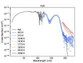
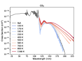
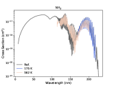
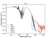
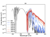
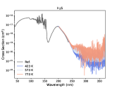
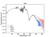
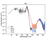
Figure 38: Photoabsortion cross sections of H2O, CO2, and NH3 across various temperatures, with Ref. denoting the cross sections measured at room temperature. The measured cross sections of H2O at 423 K (dot) and 573 K (cross) are noisy beyond 216 nm and we use linear fit for conservative estimate. The references of the cross sections are described in Section 2.5.

Recent work has started to investigate the high-temperatures UV cross sections of a few molecules (Venot et al., 2015, 2018). Given the available data, we have included temperature-dependent photoabsorption cross sections of H2O (EXOMOL), CO2 (Venot et al., 2018) (with 1160 K from EXOMOL), NH3(EXOMOL), O2 (Frederick & Mentall, 1982; Vattulainen et al., 1997), SH (Gorman et al., 2019), H2S (Gorman et al., 2019), COS (Gorman et al., 2019), CS2 (Gorman et al., 2019) in the current version of VULCAN. The temperature dependence of the UV cross sections of these molecules can be found in Figure 38. It is evident that both the absorption threshold and cross sections of CO2 exhibit strong temperature dependence. For H2O, we have incorporated the recent measurement for the cross section above 200 nm (Ranjan et al., 2020). We follow Ranjan et al. (2020) taking a log-linear fit for the noisy data above 216 nm. In addition, we have included measured data from Schulz et al. (2002) for temperature above 1500 K, .

A layer-by-layer interpolation for the temperature-dependent cross sections is implemented in the model, i.e. the cross section of one single species is allowed to vary across the atmosphere due to the temperature variation. The interpolation is linear in the temperature space and logarithmic in the cross-section space. With limited data, we find the linear interpolation in temperature generally underestimates the cross sections and therefore our implementation is considered as a conservative estimate for how photolysis increases with temperature.

2.6 Condensation and rainout

VULCAN handles condensation and evaporation using the growth rate of particles, assuming sufficient activated nuclei. For a schematic condensation/evaporation reaction

$$\ce{A_{(gas)}<->A_{(particle)}},$$ (13)

the reaction rate is given by the mass balance equation (Seinfeld & Pandis, 2016)

$$\frac{dn_{\textrm{A}}}{dt}=-\frac{D_{\ce{A}}m_{\ce{A}}}{\rho_{p}r_{p}^{2}}(n_{\ce{A}}-n^{\textrm{sat}}_{\ce{A}})n_{\ce{A}}$$ (14)

where $D_{\ce{A}}$ and $m_{\ce{A}}$ are the molecular diffusion coefficient and molecular mass of gas A, $\rho_{p}$ and $r_{p}$ are the density and radius of the particle, $n_{\ce{A}}$ and $n^{\textrm{sat}}_{\ce{A}}$ are the number density and saturation number density of gas A, respectively. Equation (14) describes the growth rate by diffusion for particles with size $r_{p}$ in the continuum regime (particles larger than the mean free path i.e. Knudsen number ($K_{n}$) smaller than 1). The negative value of Equation (14) corresponds to condensation when $n_{\ce{A}}>n^{\textrm{sat}}_{\ce{A}}$ and the positive value corresponds to evaporation when $n_{\ce{A}}<n^{\textrm{sat}}_{\ce{A}}$. Our condensation expression takes the same form as Hu et al. (2012); Rimmer & Helling (2016), except that the growth rate of particles in the kinetic regime (particles smaller than their mean free path i.e. Knudsen number ($K_{n}$) greater than 1) is used in Hu et al. (2012); Rimmer & Helling (2016). When applying $K_{n}=\frac{\pi\mu v_{th}}{4P}$ where $\mu$ is the dynamic viscosity, $v_{th}$ the thermal velocity, and $P$ the pressure, a H2 atmosphere enters the kinetics regime with $K_{n}>10$ above 1mbar for a temperature of 400 K and above 0.1 $\mu$bar for a temperature of 1000 K. We find that for most of the application, condensation occurs in the lower atmosphere with micron-size or larger particle and the continuum regime is more suitable. Since condensation typically operates in a relatively short timescale, we implement an option to switch off condensation and fix the abundances of condensing species and the condensates after the dynamic equilibrium has reached. The approach is similar to the quasi-steady-state assumption (QSSA) method, which decouples the fast and slow reactions to ease the computational load.

After the gas condenses to particles, they fall following the terminal settling velocity ($v_{s}$) derived from the Stoke’s law (Seinfeld & Pandis, 2016) as

$$v_{s}=\frac{2}{9}\frac{\rho_{p}r_{p}^{2}g}{\mu}$$ (15)

where $\mu$ is the atmospheric dynamic viscosity with value taken from Cloutman (2000) for the corresponding background gas. We have again assumed large particle size to simplify the slip correction factor (the correction for non-continuum) to unity in Equation (15). In this work, we have implemented and will demonstrate the condensation of H2O, NH3, S2, and S8 in the following sections.

2.7 Chemistry of Ti and V Compounds

TiO (titanium oxide) and VO (vanadium oxide) are present in the gas phase in cool stars and brown dwarfs where temperature exceeds 2000 K. The highly irradiated hot Jupiters have been suggested to manifest inverted temperature structures due to the strong optical absorption of TiO and VO vapor (Hubeny et al., 2003) in the stratosphere. The pioneering work proposing the role of TiO and VO in irradiated atmosphere (Fortney et al., 2008) is based on equilibrium chemistry, where the authors argue that the conversion between TiO and TiO2 is fast enough for TiO to remain in chemical equilibrium. However, it is not clear for conversion reactions with Ti or other titanium species. For example, the interconversion of CO ¡-¿ CO2 is relatively fast but the ultimate CO abundance is still controlled by the slower CO ¡-¿ CH4 interconversion. In addition to TiO, titanium hydride (TiH), has been suggested important in brown dwarfs by Burrows et al. (2005). As the thermodynamics data of TiH is not available in the literature or standard databases, Burrows et al. (2005) perform ab initio calculations of the Gibbs free energy of TiH (based on the partition function obtained from the spectroscopic constants). To explore the kinetics of titanium and vanadium, we expand the species list to include Ti, TiO, TiO2, TiH, TiC, TiN, V, VO. As only Ti, TiO, and TiO2 are available for titanium compounds in the NASA polynomials, we adopt the thermodynamics data of TiH from Burrows et al. (2005), TiC from Woitke et al. (2018), and the rest from Tsuji (1973).

While there are a few measurements for the reactions of titanium/vanadium species with laser vaporization at low temperature, the kinetics data at high temperature is nearly non-existent. As a first step, we perform simple estimates on the unknown rate constants of titanium/vanadium species. First, we look for kinetics data of analogous transition metals, such as Fe. We assume the same rate coefficient as the analogous reaction if it is measured at high temperature. When high-temperature data are not available, we estimate the temperature dependence based on transition state theory. For an endothermic reaction, we approximate the activation energy (the exponential term in the Arrhenius expression) by the enthalpy difference between the products and reactants, assuming the energy increase of the transition state is small compared to the enthalpy difference for reactions involving radicals . Once the activation energy is obtained, the pre-exponential factor is adjusted to fit the reference value at low temperature. The titanium/vanadium kinetics we adopted is listed in Table 5. For photolysis, we include photodissociation of TiO, TiO2, TiH, TiC, and VO. We estimate their UV cross sections from FeO (Chestakov et al., 2005) at 252.39 nm and scale the photolysis threshold according to their bond dissociation energy.

2.8 Photochemical Hazy Precursors

Observations have informed us that clouds or photochemical hazes are ubiquitous in a diverse range of planetary atmospheres. Microphysics models that include processes such as nucleation, coagulation, condensation, and evaporation of particles (e.g., Gao & Benneke, 2018; Kawashima & Ikoma, 2019; Lavvas & Koskinen, 2017) simulate the formation and distribution of various-size aerosol particles. Given the complexity and uncertainty of the polymerizing pathways, one common approach is to select precursor species as a proxy and assume they will further grow into complex hydrocarbons (Morley et al., 2013; Kawashima & Ikoma, 2018). Typical choices of haze precursors include C2H_x and HCN, which is also limited by our kinetics knowledge and computing capacity.

In this work, we preferentially consider precursors that are more closely related to forming polycyclic aromatic hydrocarbon (PAH) or nitriles. PAH is a group of complex hydrocarbon made of multiple aromatic rings, which has been commonly found in the smog pollution on Earth and expected to be associated with the organic haze on Titan (Zhao et al., 2018). In the polar region of Jupiter where charged particles are the main energy source, ionchemistry has also been suggested to promote the formation of PAHs and organic haze (Wong et al., 2003). Once the first aromatic ring, benzene, has formed, the thermodynamics state (enthalpy and entropy) does not vary much with the processes of attaching and arranging the rings. From the kinetics point of view, the classic mechanism of making complex hydrocarbons, H-Abstraction-Carbon-Addition (HACA), requires aromatic hydrocarbon and acetylene in the primary abstraction and addition steps (e.g. Frenklach & Mebel, 2020). It is conceivable that benzene formation is the rate-limiting step in forming complex hydrocarbons as the growth rate increases downstream from benzene. In practice, while the fundamental pathways leading to PAH remain elusive (Wang, 2011; Zhao et al., 2018), the combustion study can provide a good handle on the formation of benzene to a certain degree. Therefore, we suggest considering benzene as an important haze precursor.

One important caveat about modeling benzene is that its photodissociation branches are poorly quantified across various branches (see e.g. Lebonnois, 2005). The main photolysis products are possibly phenyl radical (C6H5) and benzyne radical (C6H4) (Suto et al., 1992). If they further absorb photons again, they could fragment into smaller, linear molecules like C4H3 and C3H3. We adopt the cross sections of C6H6 from Boechat-Roberty et al. (2004) and Capalbo et al. (2016). For simplicity, we assume the main dissociation of benzene primarily goes into phenyl radical (C6H5) with a small fraction leading to C3H3 ($\sim$ 15$\%$ based on (Kislov et al., 2004)).

Although HCN is the basic molecule for nitrile chemistry, it is unlikely that most of HCN will convert into complex nitriles. The nitrile formation is more likely to be limited by the less abundant H2CN, CH2NH, or CH3CN. Hence we include these species along with HC3N to represent the nitrile family precursor. For sulfur gases, in addition to the condensation of sulfur allotropes (S_x), we also consider CS2 according to the laboratory experiments by He et al. (2020). Overall, we compose the following species as photochemical haze precursors: C2H2, C2H6, C4H2, C6H6, HCN, HC3N, CH2NH, CH3CN, CS2.

3 Model Validation

Table 1: Model Validation Setup

Planet	P-T profile	Network	stellar UV	Gravity	Upper Boundary	Lower Boundary
				(cm2/s)
HD 189733b	Moses et al. (2011)	N-C-H-O	Eps Eri	2140	H escape	zero-flux
Jupiter	Moses et al. (2005)	N-C-H-O-lowT	Gueymard (2018)	2479	H2O, CO, CO2	zero-flux
	+ dry adiabat				inflow
Earth	COSPAR	S-N-C-H-O-full	Gueymard (2018)	980	H, H2 escape	Table 2

3.1 HD 189733b

We have benchmarked our thermochemical kinetics results using a C-H-O network with vertical transport against Moses et al. (2011) for HD 189733b and HD 209458b in Tsai et al. (2017). In this work, we compare our results including N-C-H-O photochemistry to Moses et al. (2011) and Venot et al. (2012) (M11 and V12 hereafter). V12 use a chemical kinetics scheme derived from combustion application and find different disequilibrium abundances of CH4 and NH3 from those in M11. Since then, a size-reduced network based on V11 has been developed (Venot et al., 2019), with the motivation to support computationally heavy simulations. In particular, the controversial methanol mechanism, which has been identified to cause the differences in CH4-CO conversion (Moses et al., 2011; Moses, 2014), is further updated and analyzed in (Venot et al., 2020). Therefore, aiming to consolidate the model discrepancy, we run an additional model with VULCAN but implemented with the updated reduced network from Venot et al. (2020). The planetary parameters and model setting are listed in Table 1. Before diving into the detailed comparison, we provide an overview of the chemical profiles and absorption properties for HD 189733b and HD 209458b in Figure 1.

3.1.1 Disequilibrium Effects

The left panels of Figure 1 depict how vertical mixing and photochemistry drives the compositions out of equilibrium on HD 189733b, by isolating the two effects. The underlying processes can be understood as a general property of hot Jupiters, as discussed in (Moses et al., 2011; Venot et al., 2012; Moses, 2014; Hobbs et al., 2019; Molaverdikhani et al., 2019). Equilibrium chemistry prevails in the deep, hot region whereas energetic photons dissociate molecules and produce reactive radicals in the upper atmosphere. Between the two regions, the composition distribution is controlled by vertical transport, viz., species in equilibrium at depth are transported upward and become quenched when vertical mixing predominates chemical reactions; photochemical products are also mixed downward and initiate a sequence of reactions.

The right panels of Figure 1 show the UV photosphere where the optical depth equals one, with decomposition of contribution from the main molecules. Our photochemical model captures several general transmission properties of irradiated H2-atmospheres: H2 provides the dominant absorption in EUV (10–120 nm) whereas H2O and CO are the dominant absorbers in FUV (120–200 nm). The window around 160–200 nm is particularly important for water dissociation, which makes a catalytic cycle turning H2 into atomic H (Liang et al., 2003; Moses et al., 2011). In the NUV (300–400nm), radiation can penetrate deep down to $\sim$ 1 bar until being scattered. The photospheres in Figure 1 descend from about 1 $\mu$bar to 10 mbar (from the end of H2-shielding to the tail of ammonia absorption) which denote the photochemically active region in the atmosphere.

HD 209458b shares qualitatively similar results with HD 189733b. Owning to its higher temperature and the inverted thermal structure (see Figure 1. in Moses et al. (2011)), the quench level is lifted higher and the photolysis has little influence, as can be seen in Figure 1. The composition distribution on HD 209458b can be described by a lower equilibrium region and an upper quenched region. We will now only focus on HD 189733b for the model comparison as disequilibrium processes contribute more compared to the hotter HD 209458b (see Hobbs et al. (2019) for model comparison of HD 209458b).

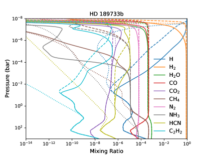
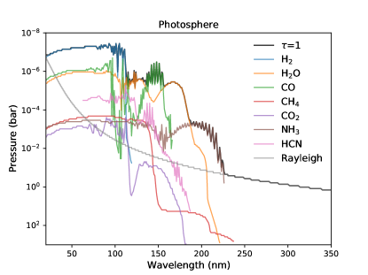
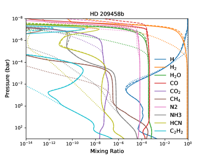
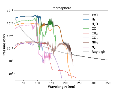
Figure 1: C-H-N-O Photochemical kinetics results (top-left) of HD 189733b (solid), compared with including vertical mixing but no photochemistry (dashed), and thermochemical equilibrium (dotted). The temperature-pressure structure and eddy diffusion (K_zz) profile are taken from the dayside-average profile in Moses et al. (2011) (their Figure 1 and 2). On the top right, we show the pressure level where energetic photons are mostly absorbed, i.e. optical depth $\tau$ = 1 (black), and decomposed into the main absorbers. The bottom panels show same as the top panels except for HD 209458 b.

3.1.2 Model Comparison with Moses et al. (2011) and Venot et al. (2012)

The HD 189733b model comparisons between VULCAN, M11, and V12 are showcased in Figure 2, where the top row highlights the major species and the following rows are grouped into carbon, oxygen, and nitrogen species. For the major species, VULCAN produces profiles more consistent with M11, while there are notable differences with V12 in H, CH4, NH3, and HCN. CH4 and NH3 are quenched from below 1 bar level until being attacked by H around 1 mbar. Hence the differences with V12 in the photospheric region ($\sim$ 1 bar – 1 mbar) are due to thermochemical kinetics, rather than photochemical sources. Nitrogen species generally manifest higher variances, reflecting the kinetics uncertainties.

Quenching of CH4 and NH3

The sharp gradients of the equilibrium distribution of CH4 and NH3 (Figure 1) imply the abundances are sensitive to the quench levels, viz. small differences in the quench levels can lead to considerable differences. The key reactions responsible for the conversion at quench levels deserve a closer look.

The match of quenched CH4 abundance between VULCAN and M11 has been discussed in Tsai et al. (2017), in which we identify a similar pathway of CH4 destruction as M11. The inclusion of nitrogen does not change the fact since nitrogen does not participate in the CH4-CO conversion. It can be seen that CH4 is quenched at a higher level with lower mixing ratio in V12, as a result of faster CH4-CO conversion. Moses (2014) identified the faster methanol decomposition H + CH3OH -¿ CH3 + H2O measured by Hidaka et al. (1989) adopted in V12 as the key reaction that CH4 exhibits a shorter timescale in V12. Moses (2014) suggested the rate is overestimated by Hidaka et al. (1989) based on the high energy barrier of the reaction. In response, Venot et al. (2019) removed the controversial reaction by Hidaka et al. (1989) and updated their chemical scheme with a newly validated CH3OH combustion work (Burke et al., 2016), given the importance of methanol as an intermediate species for CH4-CO conversion. Intriguingly, Venot et al. (2019) still find a methane abundance rather close to that in V12.

Attempting to resolve this mystery, we further run our model with the Venot et al. (2020) reduced scheme integrated with new CH3OH mechanism. We did not incorporate the same photolysis scheme from V12 but here photolysis has no effects on the quenching comparison below 1 bar. Contrary to the findings in Venot et al. (2020), the new scheme of Venot et al. (2020) implemented in our model indeed shows a slower CH4-CO conversion and brings the CH4 profile closer to VULCAN and M11 (dotted line in Figure 2-(b)). Our model implemented with the Venot et al. (2020) scheme predicts a quenched methane mixing ratio 1.13 $\times 10^{-5}$, close to 1.51 $\times 10^{-5}$ in M11 and 1.26 $\times 10^{-5}$ in our nominal model, whereas V12 with the faster methanol decomposition from Hidaka et al. (1989) predicts 5.20 $\times 10^{-6}$. We conclude that the methanol decomposition indeed results in faster CH4-CO conversion and subsequently lowers the CH4 abundance in V12.

For nitrogen chemistry, the high-temperature kinetics is more uncertain and many reducing reactions relevant for H2-atmospheres are not available on the NIST database. We drew data from the combustion literature (Dean & Bozzelli (2000), same as M11) and the KIDA database. In particular, there are considerable uncertainties regarding the rates for the reactions that control the NH3-N2 conversion, as extensively discussed in Moses (2014). We follow the suggestions in Moses (2014) and adopt the rate coefficient of NH3 + NH2 -¿ N2H3 + H2 from Dean et al. (1984) and that of NH2 + NH2 -¿ N2H2 + H2 from Klippenstein et al. (2009), since Konnov & De Ruyck (2001) used in V12 is measured at low temperatures.

As NH3 progressively become fully quenched in the region between a few hundreds bar and 1 bar, there are more than a single pathway and rate-limiting step for NH3-N2 conversion that effectively control the NH3 abundance. For pressure greater than $\sim$ 30 bar, we identify the pathway

$$\begin{aligned} \ce{NH3+H&->NH2+H2}\\ \ce{NH3+NH2&->N2H3+H2}\;(\textrm{i})\\ \ce{N2H3&->[\textrm{M}]N2H2+H}\;(\textrm{ii})\\ \ce{N2H2+H&->N2H+H2}\\ \ce{N2H&->[\textrm{M}]N2+H}\\ \vglue 5.0pt\cr\hline\cr\vglue 5.0pt\cr\mbox{net}:\ce{2NH3&->N2+3H2}.\end{aligned}$$ (16)

where the rate-limiting step switches from (16)-(i) to (16)-(ii) with increasing pressure. In the region with pressure between 30 and 1 bar, we find two pathways with close contribution:

$$\begin{aligned} 2(\ce{NH3+H&->NH2+H2})\\ \ce{NH2+H&->NH+H2}\\ \ce{NH+NH2&->N2H2+H}\;(\textrm{iii})\\ \ce{N2H2+H&->N2H+H2}\\ \ce{N2H&->[\textrm{M}]N2+H}\\ \ce{H2&->[\textrm{M}]2H}\\ \vglue 5.0pt\cr\hline\cr\vglue 5.0pt\cr\mbox{net}:\ce{2NH3&->N2+3H2}.\end{aligned}$$ (17)

and

$$\begin{aligned} \ce{NH3+H&->NH2+H2}\\ \ce{NH2+H&->NH+H2}\\ \ce{NH+H&->N+H2}\\ \ce{NH3+N&->N2H+H2}\;(\textrm{iv})\\ \ce{N2H&->[\textrm{M}]N2+H}\\ \ce{H2&->[\textrm{M}]2H}\\ \vglue 5.0pt\cr\hline\cr\vglue 5.0pt\cr\mbox{net}:\ce{2NH3&->N2+3H2}.\end{aligned}$$ (18)

where (17)-(iii) and (18)-(iv) are the rate-limiting steps.

Our pathways (16) and (17) are identical to those in M11 ((5) and (6) in Moses et al. (2011)), although we find (16)-(i) still play a role for controlling NH3 quenching, even with the high energy barrier given by Dean et al. (1984). As we adopt the same rates for several key reaction relevant for NH3-N2 conversion, our model reproduces NH3 very close to M11, whereas V12 with a faster NH3-N2 conversion predicts a higher quench level and lower abundance for NH3 (Figure 2-(b)). In all, we reiterate that further investigation for the key reactions (e.g., (16)-(i), (16)-(ii), (17)-(iii), (18)-(iv)) at high temperatures are required to improve our ability to accurately model the NH3-N2 system.

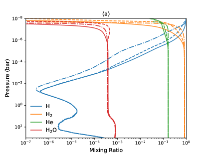
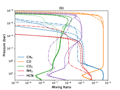
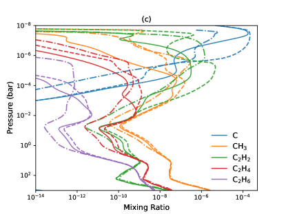
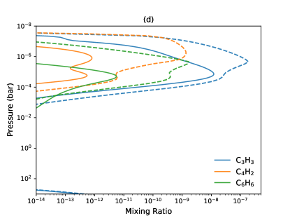
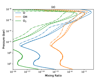
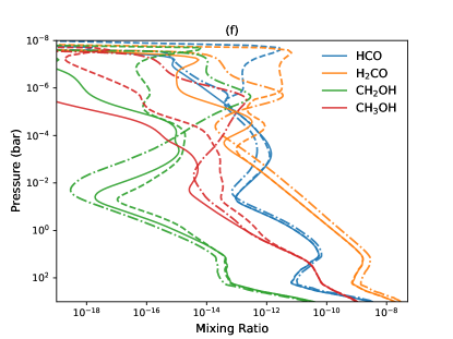
Figure 2: Comparison of atmospheric compositions on HD 189733b computed by VULCAN (solid), Moses et al. (2011) (dashed), and Venot et al. (2012) (dashed-dotted), showing volume mixing ratios of main species ((a), (b)), carbon species ((c), (d)), oxygen species ((e), (f)), and nitrogen species ((g),(h)) (some species not included in V12). Additionally, dotted lines for CH4 and CO2 are from running VULCAN with the updated methanol scheme from Venot et al. (2020).

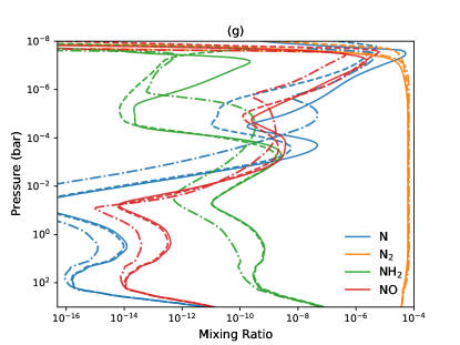
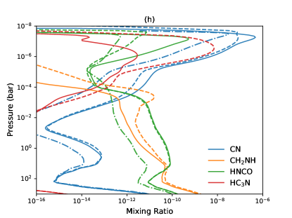
Figure 2: (cont.)

Production of CO2 and HCN

Another unexpected change in Venot et al. (2020) is that CO2 remains in chemical equilibrium across the atmosphere. Our model with the implementation of Venot et al. (2020) scheme confirmed the same result. This is remarkably differed from all other models, including V12, where CO2 is enhanced by photochemically produced OH:

$$\vspace{-0.2cm}\ce{CO+OH->CO2+H}\vspace{+0.03cm}$$ (19)

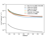
Figure 41: Comparisons of selective rate constants of Reaction (19): CO + OH -¿ CO2 + H with wide temperature ranges available on NIST.

This reaction with the OH radical is expected to rapidly convert CO into CO2 while the reaction rate is well studied owning to its importance in the terrestrial atmosphere as well as combustion kinetics. The rate coefficient of Reaction (19) adopted in Venot et al. (2020): 2.589 $\times$ 10^-16 ($T$/300)^1.5 exp(251.4 / $T$), has a pre-exponential factor about two orders of magnitude smaller than the typical values listed on NIST, as compared in Figure 41. The slow CO oxidation shuts off the CO2 production and makes CO2 retain chemical equilibrium in Venot et al. (2020). We are not sure if this rate constant is part of the updated methanol scheme from Burke et al. (2016) at this point, as to our knowledge, the base network in Burke et al. (2016) takes the rate coefficient of Reaction (19) from Joshi & Wang (2006), which is consistent with the literature and faster than that in Venot et al. (2020).

The dissociation of CH4 and NH3 leads to the formation of HCN, the primary photochemical product that coupled carbon and nitrogen on HD 189733b. HCN becomes the most abundant carbon-bearing molecule next to CO in the upper atmosphere. We identify the pathway in the HCN-dominated region between 1 mbar and 1 $\mu$bar as

$$\begin{aligned} \ce{CH4+H&->CH3+H2}\\ \ce{NH3+H&->NH2+H2}\\ \ce{NH2+H&->NH+H2}\\ \ce{NH+H&->N+H2}\\ \ce{CH3+N&->H2CN+H}\\ \ce{H2CN+H&->HCN+H2}\\ 2(\ce{H2O&->[h\nu]OH+H})\\ 2(\ce{OH+H2&->H2O+H})\\ \vglue 5.0pt\cr\hline\cr\vglue 5.0pt\cr\mbox{net}:\ce{CH4+NH3&->HCN+3H2}\end{aligned}$$ (20)

, which is identical to (14) of Moses et al. (2011). HCN in V12 naturally follows the more scarce CH4 and NH3 and presents in a lower abundance. We note that Pearce et al. (2019) have run simulations and discovered previous unknown rate coefficients, e.g., the destruction of HCN by reacting with the excited N(^2D) could be an important sink of HCN.

Photolysis Effects

In the upper stratosphere above 1 mbar, the model differences most likely come from photochemical sources. However, it is less straightforward to compare model discrepancy originated from photochemistry as each step in converting photon fluxes into photolysis rates can give rise to deviation, including stellar fluxes, cross sections, branching ratios, and radiative transfer, etc. For simplicity, we will directly inspect the computed photolysis rates from M11, V12, and VULCAN. We limit our comparison to water photolysis, owing to its importance of producing H radicals and the frontline role of H in reacting with molecules such as CH4 and NH3 (Liang et al., 2003; Moses et al., 2011).

Figure 3 compares the photodissociation rates of the main branch H2O -¿[hν] OH + H computed by three models. The water photodissociation rate in VULCAN is about twice as large as that in M11 and around one order of magnitude larger than that in V12. The H2O photolysis rates evidently correlate with the H and OH profiles in Figure 2-(a), -(e) and molecules in V12 (e.g. CH4) generally tend to survive toward higher altitude. The disagreement started even from the top of the models, with the same deviation also found across other photolytic species, such as CH4 and NH3. This implies the model implementation of stellar fluxes is the first-order contribution to photochemical differences. Although according to Venot et al. (2012), they found no differences in switching to the same stellar flux from M11 and suggested that Rayleigh scattering could be the source of disagreement. We have tested switching off Rayleigh scattering and found negligible changes, since Rayleigh scattering only dominates in the deep region where photochemistry has ceased (see Figure 1). We note that potential errors with insufficient spectral resolution can contribute to the photolysis rates as well (see Appendix B). Overall, more attention should be paid to calibrating the stellar irradiation for future photochemical model benchmarks and we suggest using H2O photolysis as a baseline.

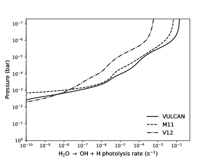
Figure 3: Comparison of the photodissociation rates (s^-1) of the main branch of H2O in HD 189733b computed by VULCAN, M11 (Moses et al., 2011), and V12 (Venot et al., 2012).

Carbon Species Comparison

Panels (c) and (d) in Figure 2 show the same comparison for other important carbon-bearing species. Atomic carbon is liberated from CO photodissociation near the top atmosphere. CO photolysis appears to be stronger in M11 and generates more atomic carbon around $\mu$bar level. The carbon vapor exceeds saturation and can potentially condense in the upper atmosphere. We will examine the implication of C condensation in Section 4.2.3. In the lower stratosphere, various hydrocarbon production is initiated by methane abstraction, i.e. H being successively stripped from CH4 to form more reactive unsaturated hydrocarbons. The hydrocarbon profiles predicted by M11, V12, and our model are consistent with the divergence of parent CH4, except that acetylene (C2H2) is also governed by atomic C in the upper atmosphere.

C2H2 is the most favoured unsaturated hydrocarbon on HD 189733b. In the CO-photolysis region, atomic C can couple with nitrogen into CN and eventually produce C2H2 by dissociation of HC3N. Yet we find CH4 to still be the dominant source for producing C2H2 below 1 $\mu$bar via a pathway such as

$$\begin{aligned} 2(\ce{CH4+H&->CH3+H2})\\ \ce{CH3+H&->CH2+H2}\\ \ce{CH2+H&->CH+H2}\\ \ce{CH+H&->C+H2}\\ \ce{CH3+C&->C2H2+H}\\ 2(\ce{H2O&->[h\nu]H+OH})\\ 2(\ce{OH+H2&->H2O+H})\\ \vglue 5.0pt\cr\hline\cr\vglue 5.0pt\cr\mbox{net}:\ce{2CH4&->C2H2+3H2}.\end{aligned}$$ (21)

Our scheme predicts C2H2 with the maximum abundance a few factor smaller than V12 and about an order-of-magnitude smaller than M11.

Ethylene (C2H4) is the next most abundant hydrocarbon after acetylene and peaks around 10 mbar. C2H4 and other C2H_x production stems from CH3 association reaction via the pathway

$$\vspace{-2cm}\begin{aligned} \ce{H2O&->[h\nu]H+OH}\\ \ce{OH+H2&->H2O+H}\\ 2(\ce{CH4+H&->CH3+H2})\\ \ce{CH3+CH3&->[M]C2H6}\\ \ce{C2H6+H&->C2H5+H2}\\ \ce{C2H5&->[M]C2H4+H}\\ \vglue 5.0pt\cr\hline\cr\vglue 5.0pt\cr\mbox{net}:\ce{2CH4&->C2H4+2H2}\end{aligned}\vspace{-0.5cm}$$ (22)

, where forming C2H6 is usually the rate-limiting step. The abundances of C2H4 and C2H6 in our model are in agreement with M11 within an order of magnitude.

The kinetics beyond C₂ hydrocarbons becomes less constrained (Moses et al., 2011; Venot et al., 2015). As discussed in Section 2.3, we intended to capture the major pathways of producing C6H6 as a proxy for haze precursors without invoking an exhaustive suite of hydrocarbons. In our model, C6H6 is formed by the pathway

$$\begin{aligned} 9(\ce{H2O+h$\nu$->H+OH})\\ 9(\ce{OH+H2->H2O+H})\\ 6(\ce{CH4+H->CH3+H2})\\ 4(\ce{CH3+H->CH2+H2})\\ 4(\ce{CH2+H->CH+H2})\\ 4(\ce{CH+H->C+H2})\\ 2(\ce{CH3+C->C2H2+H})\\ 2(\ce{C+C2H2->C3H2})\\ 2(\ce{C3H2+H+M->C3H3+M})\\ \ce{C3H3+C3H3+M->C6H6+M}\\ \hline\cr\mbox{net}:\ce{6CH4->C6H6+9H2}.\end{aligned}$$

where the recombination of C3H3 is the rate-limiting step (akin to the cooler atmosphere of Jupiter (Moses et al., 2005)). Figure 2-(d) shows that C4H2 and C6H6 predicted by our reduced scheme have considerably lower abundances than those in M11. Given the agreement of C3H3 up until 10^-5 bar, we suspect that the differences of C6H6 between VULCAN and M11 are due to photodissociation effects from C6H6 as well as other species such as CO. Given all the uncertainties and complexity as we mentioned in Section 2.8, we do not consider the predicted abundances of C4H2 and C6H6 to be accurate, but it should rather serve the purpose for accessing the haze precursors.

Oxygen Species Comparison

Panels (e) and (f) of Figure 2 compare oxygen-bearing species. The deviation of O, OH, and O2 again follows the discrepency in H2O photolysis, similar to H. There is a minor shift of the equilibrium abundance of H2CO in V12, possibly from the thermodynamic data difference between JANAF and the NASA polynomial, as pointed out in Tsai et al. (2017). All three models exhibit somewhat different quench levels and profiles for CH2OH and CH3OH, which are generally important intermediates for CH4-CO interconversion Moses et al. (2011); Tsai et al. (2018); Venot et al. (2020). Nevertheless, this does not reflect in the CH4 abundance since CH4 has already quenched in the deeper region. The updated methanol scheme in Venot et al. (2020) also provides more consistent CH2OH and CH3OH distributions with M11 and VULCAN. Since VULCAN adopted the same rate coefficients from the ab initio calculation from M11 for the three methanol reactions, the difference between VULCAN and M11 is more likely associated with reactions involving CH2OH.

Nitrogen Species Comparison

Panel (g) and (h) of Figure 2 compare nitrogen-bearing species. N and NH2 follow the same quench level as NH3 (panel (b)), since they are part of the NH3-N2 conversion. Considerable amount of atomic N is produced above mbar level by hydrogen abstraction of ammonia, similar to that of methane. Atomic N is oxidized by OH into NO in the upper atmosphere. NO reacts rapidly with atomic C into CN, as C-N bond is stronger than N-O bond. CN is an important source of nitrile production, e.g., CN reacts with C2H2 to form HC3N. Our model shows a slower HC3N production and predicts HC3N with a peak value about two orders of magnitude lower than M11.

The carbon-nitrogen-bearing species are grouped in Figure 2-(h). Since NH3 quenched first in the deeper layers than CH4, the quench levels of general carbon-nitrogen-bearing species also follow NH3. Despite in trace abundance, CH2NH and HNCO participate in HCN forming mechanism and become important at high pressures. We find HCN formed around 10 mbar via CH2NH and CH3NH2 in a pathway identical to (7) in Moses et al. (2011).

We conclude that we validate our model of HD 189733b by thoroughly reproducing composition distribution within the uncertainty range enclosed by M11 and V12. The kinetics data we employed generally yields quenching behavior close to M11, while our model appeared to predict lower C2H2, C4H2, C6H6, and HC3N than M11 in the upper atmosphere. Contrary to what have been reported in Venot et al. (2020), we find that the update methanol scheme in fact increases the quenched CH4 abundance and more consistent with that in M11 and this work. The photochemical part of the atmosphere is more complex to diagnose but we suggest the implementation of stellar fluxes is the main factor in the discrepancy between M11, V12, and VULCAN.

3.2 Jupiter

The modeling work for Jovian chemistry broadly falls into two categories addressing two main regions: the stratosphere and the deep troposphere. The stratospheric compositions are governed by photochemical kinetics with the main focus on understanding the formation of various hydrocarbons. For stratospheric models, fixed mixing ratios or fluxes at the lower boundary need to be specified (Yung & Strobel, 1980; Moses et al., 2005). As for the deep tropospheric compositions below the clouds with sparse observational constraints, kinetics models attempt to infer the interior water content based on other quenched species (Visscher et al., 2010; Wang et al., 2016). Since chemical equilibrium is expected to hold in the deep interior, the elemental ratio essentially controls the reservoir of gases and vertical mixing determines the quenched compositions in the upper troposphere.

In this validation, our objective is to validate the chemical scheme at low temperatures with observed hydrocarbons and verify the condensation scheme. We take a general approach by connecting the deep troposphere to the stratosphere and solve the continuity equations consistently. Our lower boundary at 5 kbar is far down in the region ruled by equilibrium chemistry and zero flux can be applied to the lower boundary. In this setup, fixed-abundance lower boundary conditions are not required as in the stratosphere models (e.g., Moses et al., 2005; Hue et al., 2018). The compositions at the lower stratosphere are physically determined by condensation and transport from the troposphere in the model.

3.2.1 Model Setup

The temperature profile in the stratosphere and top of the troposphere (above 6.7 bar) is taken from Moses et al. (2005) and extended to 5000 bar following the dry adiabat, with T = 427.71 K at 22 bar measured by the Galileo probe as the reference point. We use the same eddy diffusion profile for the stratosphere as Model A of Moses et al. (2005), which is derived from multiple observations. The eddy diffusion is assumed to be constant with 10⁸ (cm²/s) in the convective region below 6.7 bar. The temperature and eddy-diffusion profiles adopted for our Jupiter model are shown in Figure 4.

Heavy elements in Jupiter are enhanced compared to solar metallicity, except the oxygen abundance is still unclear. We assign the elemental abundances for the Jupiter model as He/H = 0.0785 (Atreya et al., 2020), C/H = 1.19$\times$10^-3 (Atreya et al., 2020), O/H = 3.03$\times$10^-4 (0.5 times solar), and N/H = 2.28$\times$10^-4 (Li et al., 2017). Sulfur is not included in our Jupiter validation for simplicity. We include condensation of H2O and NH3, assuming a single particle size with average radius equal to 0.5 $\mu$m for the cloud condensates. Oxygen sources from micrometeoroids are prescribed at the upper boundary at 10^-8 bar following Moses et al. (2005), with influx (molecules cm^-2 s^-1) of H2O = 4 $\times$ 10⁴, CO = 4 $\times$ 10⁶, and CO2 = 1 $\times$ 10⁴.

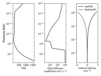
Figure 4: The temperature, eddy diffusion, and deep vertical velocities used for our Jupiter model. The temperature and eddy diffusion in the stratosphere are taken from Moses et al. (2005), while a dry adiabat and uniform eddy diffusion with $K_{\textrm{zz}}$ = 10⁸ (cm²/s) are assumed for the troposphere. The upward (positive) and downward (negative) vertical velocities are prescribed by Equation (24) with the maximum speed of 5 cm/s at 0.7 bar.

3.2.2 Comparing to Stratospheric Observations and Moses et al. (2005)

The top panel of Figure 5 displays the vertical distribution of key species computed by our model, compared to Moses et al. (2005) and various observations. First, CH4 is the major carbon-bearing species across the atmosphere. It is well-mixed until photolysis and separation by molecular diffusion take in place at low pressure. The CH4 distribution in our model matches well with the observation (Drossart et al., 1999). We verify that our treatment of molecular diffusion accurately reproduces the decrease of CH4 due to molecular diffusion above the homopause.

Second, our model successfully predicts the major C2 hydrocarbons, which stem from CH4 photolysis in the stratosphere. Our model tends to predict lower abundances for the unsaturated hydrocarbons C2H2 and C2H4 than Moses et al. (2005) in the lower stratosphere, but both profiles are within the observational constraints. The UV photosphere in Figure 5 indicates that CH4 predominates the absorption from Ly-$\alpha$ to about 150 nm. We find the main scheme of converting CH4 to C2H6 in the upper atmosphere is

$$\begin{aligned} 2(\ce{CH4&->[h\nu]CH3+H})\\ 2(\ce{CH3+CH3&->[M]C2H6})\\ \ce{2H&->[M]H2}\\ \vglue 5.0pt\cr\hline\cr\vglue 5.0pt\cr\mbox{net}:\ce{2CH4&->C2H6+H2}\end{aligned}$$ (23)

and the photodissociation branch of methane is replaced by CH4 -¿[hν] ^1CH2 + H2 followed by ^1CH2 + H2 -¿CH3 + H at higher pressures. We confirm that hydrogen abstraction and three-body association reactions are sensitive to the formation of hydrocarbons on Jupiter as discussed in detail in Moses et al. (2005). Particularly in the lower stratosphere where temperature drops below 200 K, the rate constants fall out of the valid temperature range or are not well constrained. We find it is particularly important to adopt the low-temperature rate constants for CH4 and C2Hx recombination reactions, i.e. CH3 + H -¿[M] CH4 , H + C2H2 -¿[M] C2H3, H + C2H3 -¿[M] C2H4, H + C2H4 -¿[M] C2H5, and H + C2H5 -¿[M] C2H6. We also adopt the limit of rate constants below certain threshold temperatures derived by Moses et al. (2005).

Third, our condensation scheme predicts the location of water-ice clouds starts at 3.6 bar and ammonia clouds at 0.7 bar as shown in Figure 5, consistent with the thermodynamics prediction with 0.5 solar O/H (Atreya et al., 2005; Weidenschilling & Lewis, 1973). The ammonium hydrosulfide (NH4SH) is not considered since sulfur is not included. Last, our model produces lower abundances of C4H2 and C6H6 is produced at higher altitude compared to those in Moses et al. (2005), which reflects the uncertainties in high-order hydrocarbons and the photolysis branches of C6H6.

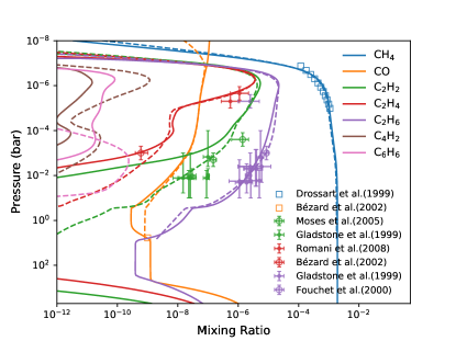
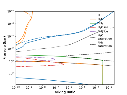
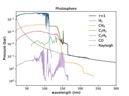
Figure 5: The top panel shows the vertical mixing profiles of important chemical species in our Jupiter model (solid), compared with various observations (data points) of hydrocarbons and the stratospheric distributions from Model A of Moses et al. (2005) (dashed). We follow Rimmer & Helling (2016) placing a factor of two error bars in pressure when they are not given in the observational data. The vapor mixing ratios and cloud densities (g/cm³) of the condensible H2O and NH3 are displayed in the middle panel. The bottom panel illustrates the UV photosphere where $\tau$ = 1 with decomposition of main absorbers.

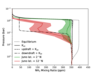
Figure 6: The deep ammonia distribution in parts per million (ppm) computed by our Jupiter model (black), while assuming chemical equilibrium, with eddy diffusion only, and including upward/downward advection for the updraft/downdraft branch (Figure 4), respectively. The red and green profiles show the inferred ammonia distribution at 2^∘ N latitude and 12^∘ N latitude based on Juno microwave measurement by Li et al. (2017), where the shaded areas enclose the 16th and 84th percentile of the samples in their MCMC runs.

3.2.3 Spatial Variation of Ammonia Due to Vertical Advection

During the Juno spacecraft’s first flyby in 2016, the microwave radiometer (MWR) on Juno measured the thermal emission below the clouds, which was inverted to global distribution of ammonia from the cloud level down to a few hundreds bar level. A plume-like feature was curiously seen associated with latitudinal variation of ammonia (Bolton et al., 2017). To explore the local impact of advection, we test how the upward and downward motion in a plume can shape the deep ammonia distribution in Jupiter.

Although Galileo probe has provided constraints on the structure of Jupiter’s deep zonal wind (Atkinson et al., 1997) and Juno also sheds light on the vertical extension of the zonal wind (Stevenson, 2020), we do not have observational constraints on the deep vertical wind. Hence we consider a simple but physically motivated (mass-conserving) vertical wind structure without tuning to fit the data. We assume an updraft and downdraft plumes starting from the bottom of NH3-ice clouds at 0.7 bar, in addition to eddy diffusion, as depicted in the right panel of Figure 4. For the non-divergent advection to conserve mass in a 1-D column, the vertical velocity at layer $j$ with number density n_j follows

$$v_{j}n_{j}=v_{\textrm{top}}n_{\textrm{top}}=\textrm{constant}$$ (24)

such that the net flux remains zero at each layer. For this test, we arbitrarily choose the maximum wind velocity at the top to be 5 cm/s. This choice has advection timescale shorter than diffusion timescale in the lower pressure region, i.e. $v_{j}$ $\gtrsim$ K${}_{\textrm{zz}}/H$, which allows us to see the influence of advection. Figure 6 compares the computed distribution of ammonia to that retrieved from Juno measurements (Li et al. (2017); also see updates in Li et al. (2020)) at two different latitudes. First, the ammonia distribution predicted by chemical equilibrium is rather uniform with depth, only slightly increasing from 350 ppm to 400 ppm. Next, vertical mixing by eddy diffusion alone makes ammonia quenched from the deep interior below 1000 bar and thus brings ammonia to a slightly lower but uniform concentration of 300 ppm. There is almost no visible difference while including the upward advection since ammonia has already been quenched by eddy diffusion from the deep region. Last, the uniform distribution of ammonia is altered in the downdraft, where the downward motion transports the lower concentration of NH3 from the condensing region. Our NH3 distribution is qualitatively consistent with the NH3-depleted branch at 12^∘ N from Li et al. (2017), where NH3 reaches a local minimum around 7 bar. We emphisize that this shape cannot be reproduced by eddy diffusion alone.

Although eddy diffusion is probably still essential in practice for parametrizing a range of mixing processes, we demonstrate that including vertical advection can be useful. The advection processes can especially play a bigger part in 2-D systems (Zhang et al., 2013; Hue et al., 2015).

3.3 Present-Day Earth

Our chemical network has only been applied to hydrogen-dominated, reducing atmospheres so far. In this section, we validate our full S-N-C-H-O network with the oxidizing atmosphere of present-day Earth. The interaction with the surface is particularly crucial in regulating the composition for the terrestrial atmosphere. Surface emission and deposition via biological and geological activities have to be taken into account. Our implementation of the top boundary fluxes and condensation scheme has been validated for Jupiter in the previous section. We will proceed to verify the lower boundary with surface emission and deposition in the Earth model.

Table 2: Lower Boundary Conditions for the Earth Validation

Species	Surface Emission	V${}_{\textrm{dep}}$
	(molecules cm-2 s-1)	(cm s-1)
CO	3.7 $\times$ 1011	0.03
CH4	1.6 $\times$ 1011	0
NO17	1.3 $\times$ 1010	0.001
N2O17	2.3 $\times$ 109	0.0001
NH317	1.5 $\times$ 109	1
NO2	0	0.01
NO3	0	0.1
SO217	9 $\times$ 109	1
H2S17	2 $\times$ 108	0.015
COS17	5.4 $\times$ 107	0.003
H2SO417	7 $\times$ 108	1
HCN	1.7 $\times$ 108	0.13
CH3CN18	1.3 $\times$ 108	0.13
HNO3	0	4
H2SO4	0	1

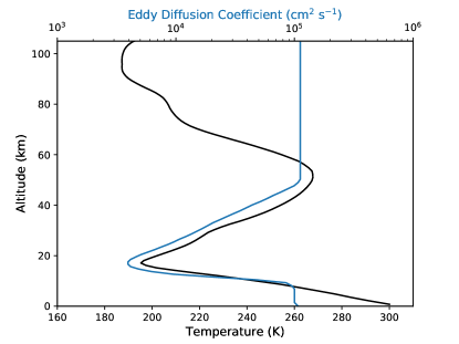
Figure 7: The temperature (at the equator in January from CIRA-86 with references described in the text) and eddy diffusion (K${}_{\textrm{zz}}$) profiles (Massie & Hunten, 1981) for the Earth model.

3.3.1 Model Setup

We follow Hu et al. (2012), taking the monthly mean temperature at the equator in January 1986 (CIRA-86) from the empirical model COSPAR International Reference Atmosphere (Rees, 1988; Rees et al., 1990) as the background temperature profile and the eddy diffusion coefficients from Massie & Hunten (1981), as shown in Figure 7. The winter atmosphere has a colder and hence drier tropopause and better represents the global averaged water vapor content (see Chiou et al. (1997) and the discussion in Hu et al. (2012)).

Unlike gas giants, terrestrial atmospheres typically do not extend to a thermochemical equilibrium region. Instead, biochemical (e.g., plants and anthropogenic pollution) and geological (e.g. volcanic outgassing) fluxes provide surface sources and sinks that are key to regulate the atmosphere. For the lower boundary condition, global emission budget provides estimates for the surface fluxes, which is conventionally recorded in the unit of mass rate (Tg yr^-1) and needed to convert to flux (molecules cm^-2 s^-1) in our 1-D model.

For Earth and any ocean worlds with large bodies of surface water reservoir, the standard setup is to fix the surface-water mixing ratio (Kasting & Donahue, 1980; Hu et al., 2012; Lincowski et al., 2018). We set the surface mixing ratio of water to 0.00894, corresponding to 25$\%$ relative humidity. Surface CO2 is also fixed at 400 ppm for simplicity, since we did not consider several major sources and sinks of CO2 at the surface, such as respiration, photosynthesis, ocean uptake, weathering, etc. The specific emission fluxes and deposition velocities for the lower boundary are listed in Table 2, while zero-flux boundary is assumed for all remaining species. We initialize the atmospheric composition with well-mixed (constant with altitude) 78$\%$ N2, 20$\%$ O2, 400 ppm CO2, 934 ppm Ar, and 0.2 ppb SO2.

For the solar flux, we adopt a recently revised high-resolution spectrum (Gueymard, 2018), which is derived from various observations and models (see Table 1. of Gueymard (2018)). The solar radiation was cut from 100 nm in Hu et al. (2012) for the missing absorption from the thermosphere. We do not find it necessary as we set the top layer to the lower thermosphere around 110 km and the EUV absorption is naturally accounted for. We have also tried including the absorption from atomic oxygen and nitrogen and found no differences regarding the neutral chemistry in the lower atmosphere, since N2 and O2 have already screened out the bulk EUV. The chlorine chemistry and lightning sources for odd nitrogen are not included in this validation.

3.3.2 Results

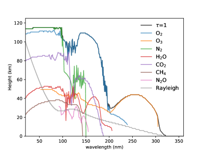
Figure 8: The UV photosphere i.e. optical depth $\tau$ = 1 (black) in our Earth model, overlaid with the composition-decomposed photosphere for several key molecules.

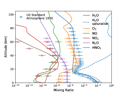
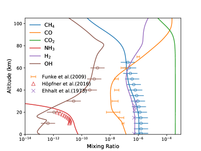
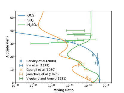
Figure 9: The global average vertical distribution of key compositions in present-day Earth’s atmosphere compared to observations. The H2O mixing ratio is from the US Standard Atmosphere 1976^*. Satellite observations of CO in the tropics and NH3 within 30^∘– 40^∘ N and 70^∘– 80^∘ E in 2003 are measured by the Michelson Interferometer for Passive Atmospheric Sounding (MIPAS) (Fischer et al., 2008). The rest unlabelled observational data are from Massie & Hunten (1981); Hudson & Reed (1979). When errors are not included in the published observations, we follow Hu et al. (2012) placing one order of magnitude error bars for the diurnal and spatial variations.

^*e.g. https://www.digitaldutch.com/atmoscalc/help.htm

Molecular oxygen (O2) and ozone (O3) are the main players in Earth’s photochemistry. O2 absorbs VUV below 200 nm and O3 takes up the radiation longward than about 200 nm, which blocks the harmful UV from life on the surface. The penetration level of solar UV flux shown in Figure 8 indicates that ozone absorbs predominately between 20 km and 50 km. The basics of oxygen–ozone cycle are described by the Chapman mechanism (e.g., Yung & DeMore, 1999; Jacob, 2011). Our full chemical network encompasses the catalytic cycles involving hydrogen oxide and nitrogen oxide radicals that are responsible for the ozone sinks in the stratosphere. Although the catalytic cycle of chlorine which accounts for additional ozone loss is not included, we are able to reproduce the observed global average ozone distribution in Figure 9.

Our condensation scheme captures the cold trap of water in the troposphere, i.e. the water vapor entering the stratosphere is set by the tropopause temperature. Above the tropopause, water is supplied by diffusion transport from the troposphere and oxidation of CH4. We find the conversion in the stratosphere go through the steps

$$\begin{aligned} \ce{CH4+OH&->H2O+CH3}\\ 2(\ce{O3&->[h\nu]O2+O(^{1}D)})\\ 2(\ce{O(^{1}D)+N2&->O+N2})\\ \ce{CH3+O&->H2CO+H}\\ \ce{O+H2CO&->HCO+OH}\\ \ce{HCO+O2&->CO+HO2}\\ \ce{CO+OH&->CO2+H}\\ \ce{HO2+OH&->H2O+O2}\\ 2(\ce{H+O2&->[M]HO2})\\ \vglue 5.0pt\cr\hline\cr\vglue 5.0pt\cr\textrm{net}:\ce{CH4+2OH+2O3&->CO2+2H2O+2HO2}\end{aligned}$$ (25)

, effectively turning one CH4 molecule into two H2O molecules (Noël et al., 2018). H2O eventually photodissociated in the mesosphere and produced H2, as indicated by the profiles in Figure 9. Overall, our model produces water distribution consistent with observations considering the diurnal and spatial variations.

The two oxides of nitrogen, NO and NO2, cycle rapidly in the presence of ozone:

$$\begin{split}\ce{NO+O3&->NO2+O2}\\ \ce{NO2+O&->NO+O2}\\ \hline\cr\mbox{net}:\ce{O3+O&->2O2}\end{split}$$

Thus NO and NO2 are conventionally grouped as NO_x. The burning of fossil fuel accounts for about half of the global tropospheric emission (e.g. Table 2.6 of Seinfeld & Pandis (2016)). NO_x is mainly lost by oxidation into nitric acid (HNO3): NO2 + OH -¿[M] HNO3. Our model reproduces distribution of NO_x, whereas our higher HNO3 in the upper stratosphere is seemingly attributed to missing the hydration removal in the actual atmosphere.

Nitrous oxide (N2O) is mainly emitted by soil bacteria, prescribed by the surface emission at the lower boundary. There is no efficient N2O removal reactions in the troposphere and N2O remains well-mixed as one of the important greenhouse gases. N2O is predominantly removed by photodissociation in the stratosphere. Our calculated N2O is in agreement with the observations for the troposphere and stratosphere. Although similar to Hu et al. (2012), our model slightly overpredicts its abundance above 50 km, which is likely due to missing the photolysis branch of N2O that produces excited oxygen O(^1S).

CH4 is the most abundant hydrocarbon in Earth’s atmosphere, with the surface emission largely comes from human activities (e.g. agriculture) as well as natural sources (e.g. wetlands). CH4 is oxidized into CO and eventually CO2 by OH through multiple steps similar to (25) in the stratosphere. CO is produced by combustion activities with about 0.1 ppm concentration near the surface Seinfeld & Pandis (2016), as a result of the balance among the emission flux, OH oxdization, and dry deposition. CO is continuously removed by OH through the troposphere and generated by photodissociation of CO2 in the thermosphere and mesosphere, as depicted by their distributions in Figure 9. As the major oxidizing agent, OH is an important diagnostic species for Earth’s photochemical model. It is mainly produced in the stratosphere during daytime initiated by ozone photolysis and regenerated in the troposphere by NO_x (see e.g., Jacob, 2011). The OH distribution in our model is consistent with that in Massie & Hunten (1981). We will further discuss using calculated OH concentration to estimate the chemical timescale of long-lived species against oxidation in the next section.

Carbonyl sulfide (OCS) is the main sulfur species in the troposphere, emitted by direct outgassing or oxidation of carbon disulfide (CS2) and dimethyl sulfide (DMS) released by the ocean (Seinfeld & Pandis, 2016; Barkley et al., 2008). OCS is rather stable in the troposphere until entering the stratosphere where it is photodissociated or oxidized by OH and ultimately turned into sulfuric acid. Sulfur dioxide (SO2) is another important sulfur containing pollutant from fossil fuel combustion. SO2 oxidation begins from the troposphere with

$$\ce{SO2+OH->[\textrm{M}]HSO3}$$

HSO3 radical rapidly reacts with oxygen to form SO3

$$\ce{HSO3+O2->SO3+HO2}$$

followed by sulfuric acid formation

$$\ce{SO3+H2O->H2SO4}$$

The sulfur-containing gases in our model generally agree with the global distribution, while the mismatch of H2SO4 is expected as our model does not include H2SO4 photodissociation and heterogeneous reactions that efficiently remove H2SO4 from the gas phase.

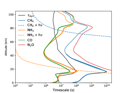
Figure 10: Calculated chemical timescales of some environmentally important gases compared to the dynamical timescale of eddy diffusion in the Earth validation model. The thick lines indicate the region where the oxidation is dominated by OH (i.e. $\tau_{\ce{OH}}$ $\simeq$ $\tau_{\ce{chem}}$).

3.3.3 Chemical Lifetime

The oxidizing capacity of Earth’s atmosphere is important for decontaminating toxic and greenhouse gases, such as CO, CH4, and various volatile organic compounds . The oxidizing power is not only essential for regulating habitable conditions but also key to address the stability of biosignature gases for other terrestrial planets. Here we present a brief overview of the key timescales for some important trace gases from our Earth model.

OH radical is the primary daytime oxidizing agent in our biosphere. The chemical timescale of species A against oxidization ($\tau^{\ce{A}}_{\ce{OH}}$) can be estimated by the computed OH concentration as

$$\tau^{\ce{A}}_{\ce{OH}}=\frac{[\ce{A}]}{k_{\ce{A}-\ce{OH}}[\ce{A}][\ce{OH}]}=\frac{1}{k_{\ce{A}-\ce{OH}}[\ce{OH}]}$$ (27)

where $k_{\ce{A-OH}}$ is the rate coefficient of the oxidizing reaction of A + OH. In the upper atmosphere where molecular collision is less frequent, the excited O(^1D) produced by ozone photolysis is not immediately stablized and becomes the main oxidant. We consider the two major oxidizing paths across the atmosphere and write the chemical timescale against oxidation as

$$\tau^{\ce{A}}_{\textrm{chem}}=\frac{1}{k_{\ce{A}-\ce{OH}}[\ce{OH}]+k_{\ce{A}-\ce{O(^{1}D)}}[\ce{O(^{1}D)}]}$$ (28)

Figure 10 illustrates the chemical timescales ($\tau_{\textrm{chem}}$) along with photolysis timescales (1/$k_{\textrm{photo}}$) for several trace gases, where $\tau_{\ce{OH}}$ (thick lines) inversely correlates with temperature in general. We can gain some insights by comparing ($\tau_{\textrm{chem}}$) to the dynamical timescale of vertical mixing ($\tau_{\textrm{dyn}}$ = H²/K${}_{\textrm{zz}}$): In the troposphere, CH4 and N2O display rather well-mixed abundances due to their longer chemical lifetime. CO and NH3 have comparable $\tau_{\textrm{chem}}$ with $\tau_{\textrm{dyn}}$ and and exhibit negative gradient with altitude from oxidation removal. In the stratosphere, NH3 is rapidly photodissociated while CH4 is transported from the troposphere and oxidized into CO. In the thermosphere above $\sim$ 80 km, the oxidation by O(^1D) takes over for most species, but mixing processes with a shorter timescale here controls the chemical distribution. For example, CO abundance starts to increase with altitude from about 60 km as a result of downward transport of CO produced by CO2 photodissociation in the upper atmosphere.

In summary, we validate our photochemical model with HD 189733b, Jupiter, and Earth, for a wide range of temperatures and oxidizing states. The inclusion of nitrogen and sulfur chemistry, along with the implementation of advection, condensation, and boundary conditions are verified by comparing with models and/or observations. The discrepancies in previous models of HD 189733b are identified for future investigation.

Table 3: Parameters of the planetary systems.

Parameter	WASP-33b	HD 189733b	GJ 436b	51 Eri b
a (AU)	0.02558	0.03142	0.02887	11.1
T${}_{\textrm{int}}$ (K)	200	—	100/400	760
R${}_{\textrm{s}}$ (R⊙)	1.51	0.805	0.464	1.45
R${}_{\textrm{p}}$ (R${}_{\textrm{J}}$)	1.603	1.138	0.38	1.11
g (cm2/s)	2700	2140	1156	18197
$\overline{\theta}$	58	48	58	67
stellar type	A5	K1-K2	M2.5	F0

4 Case study

In this section, we select WASP-33b (ultra-hot Jupiter), HD 189733b (hot Jupiter), GJ 436b (warm Neptune), and 51 Eridani b (young Jupiter) to perform case studies. Each case represents a distinctive class among gas giants with H2-dominated atmospheres. The effective temperatures of these objects span across 700–3000 K while having host stars of various stellar types. We investigate how disequilibrium processes play a part for these cases with additional attention on the effects of sulfur chemistry and photochemical haze precursors.

All the P-T profiles in this section are generated using the open-source radiative-transfer model, HELIOS, except we keep the same P-T profile of HD 189733b as in Section 3.1 for comparative purposes. HELIOS employs two-stream approximation and correlated-k method to solve for the radiative-convective equilibrium temperature consistent with thermochemical equilibrium abundances. The gaseous opacities include H2O, CH4, CO, CO2, NH3, HCN, C2H2, NO, SH, H2S SO2, SO3, SiH, CaH, MgH, NaH, AlH, CrH, AlO, SiO, CaO, CIA${}_{\ce{H2-H2}}$, CIA${}_{\ce{H2-He}}$, and additionally TiO, VO, Na, K, H- for WASP-33b. The P-T profiles are fixed without taking into account of the radiative feedback from disequilibrium chemistry (but see Drummond et al. (2016) for the effects on HD 189733b). The astronomical parameters used are listed in Table 3. The dayside-average stellar zenith angle is used for WASP-33b and GJ436b and the global-average stellar zenith angle is used for 51 Eri b (see Appendix C), except that we keep the same value for HD 189733b to compare with the results in Section 3.1. The stellar UV fluxes adopted for each system are compared in Figure 11, with detailed description in each section.

For the eddy diffusion ($K_{\textrm{zz}}$) profiles in our case studies (except that we again retain the same profile for HD 189733b from Moses et al. (2011)), we assume $K_{\textrm{zz}}$ to be constant in the convective region and increasing roughly with inverse square root of pressure in the stratosphere (Lindzen, 1981; Parmentier et al., 2013). The expression as a function of pressure in bar ($P_{\textrm{bar}}$) takes a similar form as Charnay et al. (2015) or Moses et al. (2016):

$$K_{\textrm{zz}}=K_{\textrm{deep}}(\frac{P_{\textrm{tran}}}{P_{\textrm{bar}}})^{0.4},$$ (29)

where $P_{\textrm{tran}}$ is the transition pressure level informed by the radiative transfer calculation. The more irradiated atmospheres have deeper radiative-convective transition levels and greater P${}_{\textrm{tran}}$. A common way of estimating $K_{\textrm{deep}}$ in the convective region is applying the mixing length theory with the knowledge of convective heat flux. For WASP-33b, most of the modeled atmosphere is in the radiative region. We choose $K_{\textrm{deep}}$ such that the overall pressure-dependent $K_{\textrm{zz}}$ profile matches that derived from the vertical wind in the general circulation model (GCM). For GJ 436b, $K_{\textrm{deep}}$ is treated as a loosely constrained free parameter along with the internal heating we explored (Section 4.3.1). $K_{\textrm{deep}}$ is likely more important in controlling the quenched species for cooler planets, such as 51 Eri b, where we adopted a value of $K_{\textrm{deep}}$ that can produce quenched CH4 consistent with the observations.

We run nominal models for all planets in this section with the S-N-C-H-O chemical network. We recognize there are considerable uncertainties in sulfur kinetics, as discussed in Section 2.3. In order to gauge the uncertainty effects of our sulfur scheme, we explore the sensitivity to sulfur chain-forming reactions for GJ 436b and OCS recombination for 51 Eridani b. After chemical abundances are obtained, we use the open-source tool PLATON (Zhang et al., 2019, 2020) to generate transmission spectra and HELIOS for the emission spectra.

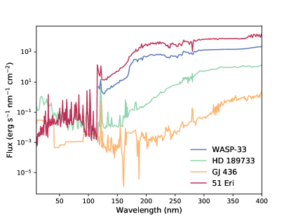
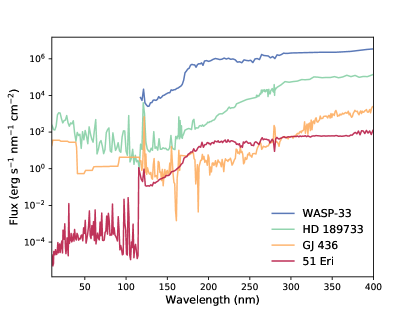
Figure 11: Stellar UV fluxes normalized at 1 AU (top) and at the top of the planet’s atmosphere (bottom) adopted in our case study models.

4.1 WASP-33b

WASP-33b is among the hottest gas giants discovered with dayside temperature around 3000 K (von Essen et al., 2020). To date it remains the only case showing evidence of both temperature inversion and TiO features (Serindag et al., 2021), which makes WASP-33b an interesting target for testing the stability of TiO/VO along with other molecules. Previous work on ultra-hot Jupiters are limited by the assumption of chemical equilibrium chemistry (Kitzmann et al., 2018; Parmentier et al., 2018; Zhang et al., 2018). Here, we will verify the equilibrium assumption by exploring how disequilibrium processes affect the titanium and vanadium compounds with different C/O ratios.

4.1.1 Stellar UV-flux and Eddy Diffusion

The host star WASP-33 is an A5 type star with effective temperature about 7400 K. We use the UV spectrum of HD 40136 (F0 type) merged with a 7000 K atlas spectrum from Rugheimer et al. (2013) as an analogue. The star is fast rotating and exhibits pulsations, which might add more uncertainties to the UV flux. Nevertheless, as we will see in Section 4.1.3, photodissociation solely converts more molecules to atoms at this high temperature and the results should be qualitatively robust.

Vertical wind generally correlates with the planet’s effective temperature (Tan & Komacek, 2019; Komacek et al., 2019; Baxter et al., 2021). We assume the value of $K_{\textrm{zz}}$ based on the simulations in Tan & Komacek (2019), where the global RMS vertical wind increases with decreasing pressure and reaches about 100 m/s at 1 mbar (personal communication). The vertical wind translates to K${}_{\textrm{zz}}$ $\sim$ 10¹¹ cm²s^-1 around 1 mbar. The temperature and eddy diffusion profiles for WASP-33b are shown in Figure 12.

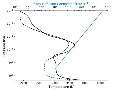
Figure 12: The temperature-pressure and eddy diffusion ($K_{\textrm{zz}}$) profiles for WASP-33b. Solar elemental abundance (solid) and C/O = 1.1 (dashed) are assumed for calculating the temperature structure.

4.1.2 Chemical Equilibrium

We first look at the trends associated with thermal dissociation governed by thermochemical equilibrium under carbon-poor and carbon-rich conditions, for which we assume a solar C/O and C/O = 1.1, respectively. Figure 13 illustrates how titanium compounds vary with temperature in equilibrium at 1 mbar. For solar C/O, titanium mainly exists in the form of Ti and TiO. As temperature exceeds about 2500 K, TiO becomes unstable against thermal dissociation and its abundance falls with temperature. For C/O = 1.1, TiO is depleted due to the scarcity of oxygen, as oxygen preferably combines with the excess carbon to form CO (Madhusudhan, 2012). Atomic titanium is the major species across this temperature range and TiC, TiH, and TiO have close abundances.

The effects of thermal dissociation on WASP-33b are clearly visible in the equilibrium profiles in Figure 14. The blistering heat of WASP-33b makes all elements predominantly exist in the atomic form above 0.1 bar, where temperature starts to increase with altitude and exceeds 3000 K, while CO with the strong C–O bond is the only molecule that survives the high temperature. For solar C/O ratio, as the majority of C is locked in CO, atomic C tracks the temperature structure whereas oxides such as H2O, TiO, VO, and TiO2 display inverse trends with temperature. For C/O = 1.1, atomic O swaps place with C and TiO and VO are significantly depleted.

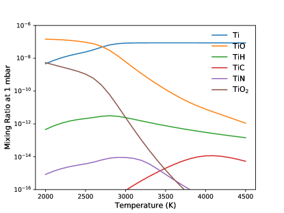
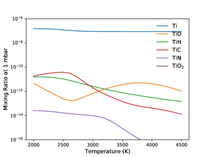
Figure 13: The equilibrium mixing ratios of several gas phase titanium species at 1 mbar as a function of temperature for solar elemental abundance (top) and C/O = 1.1 (bottom).

4.1.3 The effects of Disequilibrium Chemistry

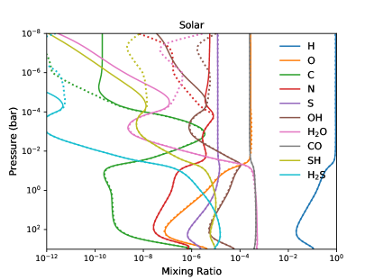
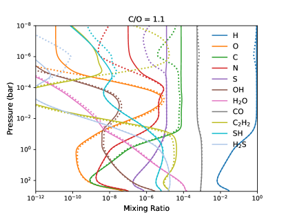
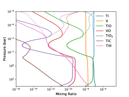
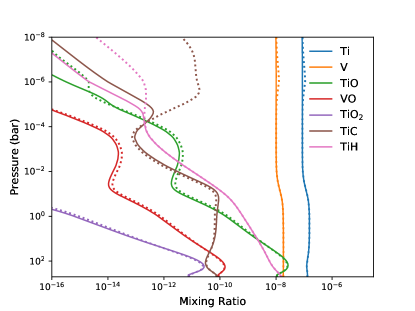
Figure 14: The composition profiles for the main species of interest for WASP-33b, assuming solar C/O (left) and C/O = 1.1 (right). The equilibrium abundances are plotted in dotted lines.

For a typical hot Jupiter (e.g. HD 189733b), vertical mixing plays a major role controlling the chemical distribution in the photosphere. However, it is not the case for WASP-33b as we compare the equilibrium and disequilibrium mixing ratio profiles in Figure 14. Although the strength of eddy diffusion also increases with temperature, faster thermochemical reactions still prevail upon vertical mixing. The deviation of disequilibrium profiles above the temperature-inverted region ( $\sim$ 10^-4 bar) is due to photodissociation, which reduces molecular species and produces more atoms. In the absence of vertical quenching, the depleted TiO in a carbon rich condition is unable to be replenished by vertical transport from the deep region, as seen in Figure 14. In the photodissociation region, in principle, stronger vertical mixing can transport more molecules upward against photodissociation. We have perform additional tests with eddy diffusion profile varied by a factor of 10. Yet we found the change is minor and our results are not too sensitive to $K_{\textrm{zz}}$.

For sulfur species, sulfur atom S is also the favored form followed by hydrogen sulfide (SH). The formation of S2 and other polysulfur (S_x) is entirely shut down at this extremely high temperature. Sulfur does not couple to oxygen, carbon, or nitrogen since it mostly remains in the atomic form. Lastly, because the adopted stellar spectrum is truncated around Lyman-$\alpha$, we have further extended the stellar spectrum to include the EUV flux shorter than Lyman-$\alpha$ using the synthetic spectra by PHOENIX . Apart from more C atoms from CO photodissociation above 10^-5 bar, we find no notable differences in all other species. Overall, the composition distribution of WASP-33b resembles that of a hot Jupiter except without a vertical quench region. The atmosphere of WASP-33b can be divided into a photochemically influenced region and a thermochemical equilibrium region, with the transition at the top of temperature-inverted layer around 10^-4 bar.

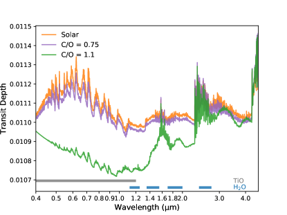
Figure 15: Synthetic transmission spectra for WASP-33b computed from modeled compositions assuming solar elemental abundance, C/O = 0.75, and C/O = 1.1. The absorption features of TiO and H2O are indicated by the color bands.

4.1.4 Transmission Spectra

We have computed the synthetic spectra from equilibrium and disequilibrium abundances and found no observable differences in both transmission and emission spectra. The photochemical region above the temperature-inverted region is too optically thin, even when molecules like H2O and TiO are strongly photodisscoiated here. High-resolution spectroscopy might be more sensitive to probe the atomic species in this region.

Alternatively, the equilibrium abundances of TiO/VO are sensitive to the change of elemental abundance. Figure 15 demonstrates that the opacity in the optical is most sensitive to the change of TiO/VO as C/O is close to unity, which shows even greater variation than H2O absorption between 1.2 and 2 $\mu$m.

In conclusion, we find photodissociation only impacts the upper atmosphere of WASP-33b where P $<$ 0.1 mbar, chemical equilibrium is generally a valid assumption, as has been found for KELT9-b (Kitzmann et al., 2018) and ultra hot Jupiters with dayside temperatures above 3000 K. Atmospheric mixing might still play an important role in an atmosphere with temperature lower than WASP-33b. Our first attempt to solve the kinetics of titanium species can provide an interesting avenue for investigating other transition metals such as Fe and Ca for future study of ultra hot Jupiters.

4.2 HD189733b

We have benchmarked our model of HD 189733b in Section 3.1, where we attempt to keep the astronomical and chemical setup as close to Moses et al. (2011); Venot et al. (2012) as possible for comparison. In this section, we include the following updates and aspects that have not been considered in previous work:
$\bullet$ Recently observed stellar UV-flux of HD 189733 (Bourrier et al., 2020)
$\bullet$ Sulfur chemistry
$\bullet$ Condensation of carbon vapor

4.2.1 Stellar UV-flux

Bourrier et al. (2020) combine HST and XMM-Newton observations and derive semi-synthetic UV spectra up to 160 nm. For our model benchmark in Section 3.1, solar flux is used for wavelengths below 115 nm and the observed spectrum of epsilon Eridani (a K2-type analogue) is adopted for 115 - 283 nm. The previously adopted and newly observed stellar fluxes are compared in Figure 16. The EUV flux of HD 189733 is modestly higher than that of the Sun, but the photochemically important FUV ($\lambda>$ 122 nm) flux appears to be weaker. Nevertheless, the change in the UV flux turns out to only slightly decrease the atomic H (by about 20$\%$). The overall impact of the updated EUV flux on neutral chemistry is in fact insignificant.

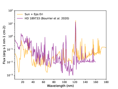
Figure 16: The UV flux of HD 189733 received at 1 A.U. derived from recent observations Bourrier et al. (2020) compared to the previously adopted spectrum, which consists of solar EUV and epsilon Eridani following the same approach as Moses et al. (2011) and used in Section 3.1. The spectra are binned for clarity.

4.2.2 Sulfur Chemistry

We next run the same model except including sulfur kinetics. The sulfur species from our photochemical calculation are illustrated in Figure 17 and are broadly consistent with previous work (Zahnle et al., 2009). Hydrogen sulfide (H2S) is the thermodynamically stable form of sulfur in a hydrogen-dominated atmosphere. H2S is mostly destroyed by hydrogen abstraction

$$\vspace{-0.1cm}\ce{H2S+H->SH+H2}\vspace{-0.1cm}$$ (30)

and restored by the reverse reaction of (30). The forward and backward reactions of (30) essentially dictates the level where H2S starts to loss its stability. On HD 189733b, H2S is dissociated above 1 mbar and predominantly turned into S. SH and S2 also reach maximum values at the level where H2S dissociation kicks off. The implication is both SH and S2 absorb shortwave radiation and could potentially provide stratospheric heating, especially with super-solar metallicity condition as discussed in Zahnle et al. (2009).

We find SO accumulated in the upper atmosphere from the oxidation of S + OH $\rightarrow$ SO + H. The highly reactive SO is known to self-react into SO dimer ((SO)2) and may facilitate formation of S2O and S2 (Pinto et al., 2021) or back into S and SO2. What actually happened in our model is SO either photodissociated or reacted with atomic H back to S in the low pressure region. The elemental S might be subject to photoionization, as we will discuss in Section 5.

One notable effect of photochemistry with sulfur is several sulfur species absorb in the MUV/NUV. As illustrated in Figure 17, sulfur species raised the UV photosphere above $\sim$ 230 nm, compared to that without sulfur where no efficient absorption beyond the ammonia bands. We find H2S responsible for the dominant absorbption in the NUV (300–400 nm), rather than SH as reported in Zahnle et al. (2009), which might be caused by the isothermal atmosphere at 1400 K used in Zahnle et al. (2009). The absorption of S2 between 250 and 300 nm and the SH peaks around 325 nm can make prospective observable features.

Figure 18 highlights the compositional differences when sulfur is present. Sulfur species can play an interesting role in catalyzing conversion schemes that take multiple steps. In particular, CH4 is more diminished down to about 1 mbar. We find sulfur provide a catalytic pathway for CH4-CO conversion. As CH4 and H2S react with atomic H to liberate carbon and sulfur, they couple to form carbon monosulfide (CS). Carbon in CS is further oxidized into OCS and eventually ends up in CO through H-abstraction, via a pathway such as

$$\begin{aligned} \ce{CH4+H&->CH3+H2}\\ \ce{CH3+H&->CH2+H2}\\ \ce{CH2+S&->HCS+H}\\ \ce{HCS+H&->CS+H2}\\ \ce{SH+H&->S+H2}\\ \ce{S+OH&->SO+H}\\ \ce{CS+SO&->OCS+S}\\ \ce{OCS+H&->CO+SH}\\ \ce{H2O&->[h\nu]OH+H}\\ \ce{SH&->[h\nu]S+H}\\ \ce{S+H2&->SH+H}\\ \vglue 5.0pt\cr\hline\cr\vglue 5.0pt\cr\mbox{net}:\ce{CH4+H2O&->CO+3H2}.\end{aligned}$$ (31)

Note there is no net change of sulfur species in the cycle. The rate-limiting reaction in pathway (33) is the carbon-sulfur step CH2 + S -¿ HCS + H, which is about three orders of magnitude faster than the pathway without sulfur around 1mbar. Interestingly, we find SH play an analogous role to H2O in catalytically converting H2 to H, causing the minor H increase in Figure 18.

The presence of sulfur species enhances the destruction of methane and might partly contribute to the scarcity of methane detection on hot Jupiters (e.g., Baxter et al., 2021, and references within). H2S has also been reported to speed up the oxidation of methane in combustion experiment (Gersen et al., 2017), in the oxidizing and high-pressure conditions of gas engines. The decreasing of CH4 naturally reduces its offspring products to a great extent. The column density shown in Figure 37 reflects the reduction of haze precursors with the participation of sulfur. Based on our fiducial analysis on HD 189733 b, we suggest that organic haze formation is likely to be partly suppressed by sulfur kinetics on a hot Jupiter, as opposed to enhanced by sulfur kinetics in a CO2-rich condition suggested by experimental simulations (He et al., 2020).

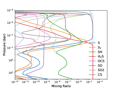
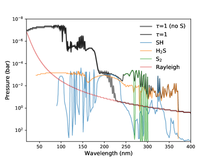
Figure 17: Left: Mixing ratios of the major sulfur species computed in the model of HD 189733b. The photochemical kinetics results are in solid lines and equilibrium abundances in dotted lines. Right: The pressure level of optical depth $\tau$ = 1 as a function of wavelength while including (black) and excluding (grey) sulfur chemistry, along with the main individual contribution from sulfur species.

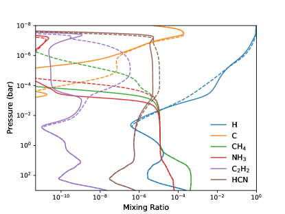
Figure 18: Mixing ratio profiles of main species on HD 189733b that exhibit differences from models including sulfur kinetics (solid) and without sulfur kinetics (dashed).

4.2.3 Condensation of Carbon Vapor

Atomic carbon vapor (C) is produced by CO dissociation (including both photodissociation and thermal dissociation in the thermosphere) or the reaction N + CN -¿ C + N2 above $\sim$ 0.1 mbar and also by H abstraction with CHx species in the lower region. The saturation vapor of C falls off rapidly with decreasing temperature in the upper atmosphere, as shown in Figure 19. In fact, the disequilibrium abundance of C starts to exceed the saturation concentration above 10 mbar. The realistic timescale for graphite growth by condensation involves detailed microphysics and is beyond the scope of this study. As a simple test, we explore the kinetic effects after carbon vapor is fully condensed. We run our HD 189733b model including sulfur chemistry and do not allow C to become supersaturated but simply fix the abundance of C in the gas phase to its saturation mixing ratio. This is physically equivalent to assuming instantaneous condensation and unlimited condensation nuclei.

Figure 19 demonstrates the consequences when C is instantaneously condensed, which mainly impacts the region above 0.1 mbar. Without the condensation of C, CH4 can be replenished by the hydrogenation sequence of C (i.e. C $\rightarrow$ CH $\rightarrow$ CH2 $\rightarrow$ CH3 $\rightarrow$ CH4). This channel is closed as C condensed out and CH4 is further depleted in the upper atmosphere. CS is reduced in the same way but C2H2 and HCN remain almost unaffected (they are already reduced compared to the model without sulfur). In the end, we find that the condensation of C has limited effects to other gas compositions in the upper atmosphere.

Figure 19: Several carbon-containing species from the nominal model (dashed) compared to those from the model with limited C due to instantaneous condensation. The saturation mixing ratio of C is plotted in dotted curve.

4.2.4 Transmission Spectra

Here we first take a look at the observational consequences due to model uncertainties among Moses et al. (2011), Venot et al. (2012), and VULCAN which we examined in Section 3.1. Figure 20 showcases the transmission spectra of HD 189733b generated from the compositions computed by VULCAN, Moses et al. (2011), and Venot et al. (2012). The lower quenched abundances of CH4 and NH3 in Venot et al. (2012) are responsible for the primary spectral differences while the spectra from VULCAN and Moses et al. (2011) are fairly close. The ammonia absorption around 8–12 $\mu$m could be a useful diagnosis for the quenching mechanism of nitrogen chemistry. Overall, we find the model uncertainties lead to about half of the spectral deviation caused by disequilibrium chemistry.

We then examine the effects of including sulfur chemistry to the transmission spectra in Figure 21. While the features from sulfur-containing species are almost obscured by other molecules such as H2O and CH4 in the near-IR, there are still visible differences due to sulfur’s impact on CH4 and NH3. Since the coupling to sulfur reduces the abundances of CH4 and NH3, the transit depth is smaller in the presence of sulfur. The differences caused by sulfur chemistry is smaller than that between equilibrium and disequilibrium CH4 and NH3 abundances but not trivial. Current observations are not capable of placing conclusive constraints and we need to rely on future facilities with higher resolving power (e.g., JWST, ARIEL).

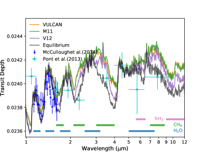
Figure 20: Synthetic transmission spectra for HD 189733b generated from chemical abundances computed by VULCAN, Moses et al. (2011), Venot et al. (2012), and when assuming chemical equilibrium. Transit observations from Pont et al. (2013) and McCullough et al. (2014) are shown as data points with error bars. The absorption features for the main molecules are indicated by the color bands.

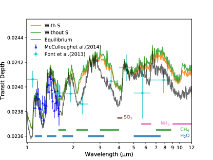
Figure 21: Same as Figure 20 but with abundances computed from our model while including or excluding sulfur species.

4.3 GJ 436b

GJ 436b is a Neptune-sized planet in a close orbit around a M dwarf star. This warm Neptune has received tremendous attention since its first discovery (Butler et al., 2004), including multiple primary transit and secondary eclipse observed with Spitzer (Stevenson et al. (2010); Madhusudhan & Seager (2011); Morley et al. (2017) and references within), as well as transmission spectroscopic study with HST WFC3 (Demory et al., 2007; Knutson et al., 2014). Spitzer 3.6 $\mu$m and 4.5 $\mu$m emission indicates the atmosphere is rich in CO/CO2 and poor in CH4. Yet precise constraint and the mechanism on CO/CH4 ratio still remain inconclusive. Forward models have suggested high metallicity (Moses et al., 2013; Morley et al., 2017) and hot interior from tidal heating (Agúndez et al., 2014) can explain the observed CO/CH4 but inconsistent with the low water content (less than 10^-4) obtained by the retrieval model Madhusudhan & Seager (2011). Hu et al. (2015) propose that a remnant helium-dominated atmosphere as a result of hydrogen escape can naturally deplete CH4 and H2O. However, the Ly-alpha absorption still appears to indicate a hydrogen-dominated atmosphere for GJ 436b (Khodachenko et al., 2019). For this work, we restrict ourself to 100 times solar metallicity (Neptune-like) and explore the effects of vertical mixing and internal heat with the presence of sulfur.

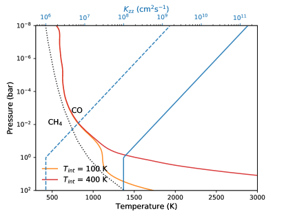
Figure 22: The temperature-pressure and eddy diffusion ($K_{\textrm{zz}}$) profiles for GJ 436b, showing low (T${}_{\textrm{int}}$ = 100 K) and high (T${}_{\textrm{int}}$ = 400 K) internal heating and weak (dashed) and strong (solid) vertical mixing. The [CH4]/[CO] = 1 equilibrium transition curve for 100 times solar metallicity is shown by the dotted curve.

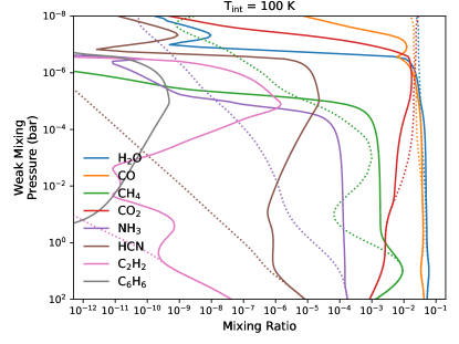
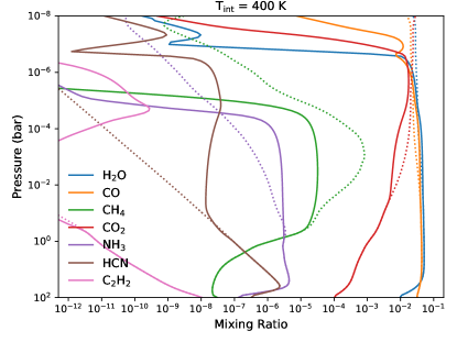
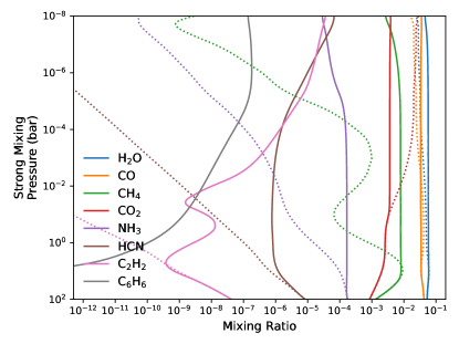
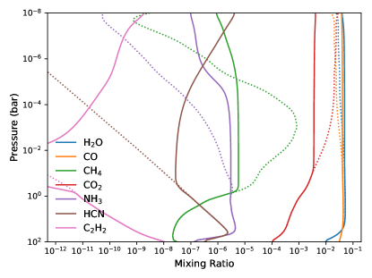
Figure 23: The mixing ratio profiles (solid) along with equilibrium profiles (dotted) of several main species on GJ 436b for different assumption of internal temperature and vertical mixing. The left/right columns correspond to low/high ($T_{\textrm{int}}$ = 100 K/$T_{\textrm{int}}$ = 400 K) internal heating and the top/bottom rows correspond to weak/strong vertical mixing.

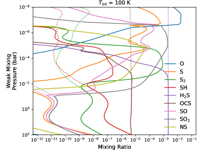
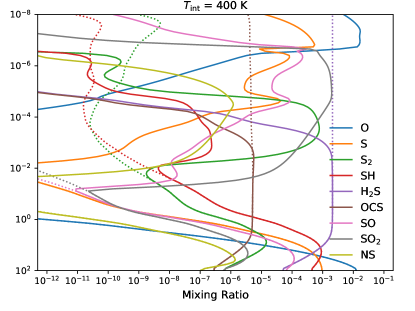
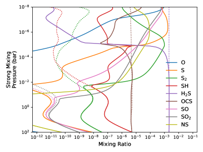
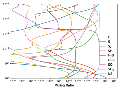
Figure 24: Same as Figure 23 but for atomic O and sulfur species.

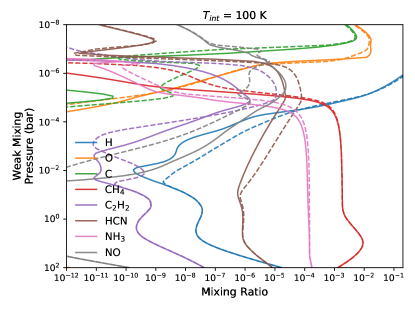
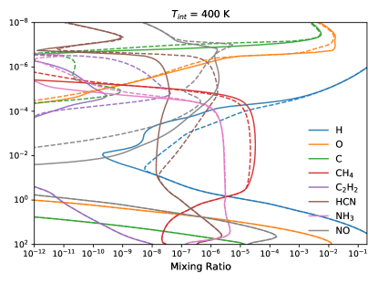
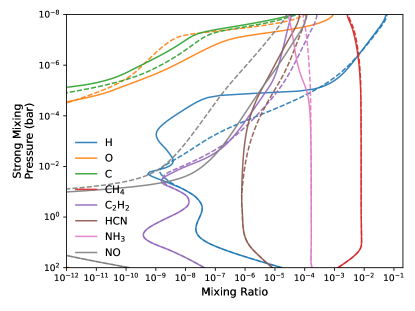
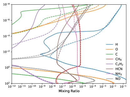
Figure 25: The abundances of several main species that show differences from models including sulfur kinetics (solid) and without sulfur kinetics (dashed). Each panel corresponds to the same internal heating and vertical mixing as Figure 23.

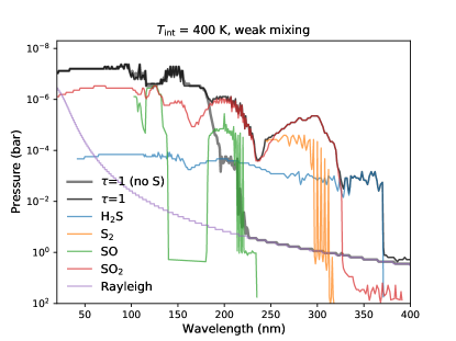
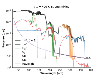
Figure 26: The pressure level of optical depth $\tau$ = 1 for GJ 436b with high internal heating (T${}_{\textrm{int}}$ = 400 K) while including (black) and excluding (grey) sulfur chemistry, along with the main contribution from sulfur species. The top and bottom panels are for weak and strong vertical mixing.

4.3.1 Model Input

Following the best-fit parameters in Morley et al. (2017), we set up a low and a high internal heating scenario by running HELIOS assuming T${}_{\textrm{int}}$ = 100 K and 400 K, respectively. The stellar UV flux of GJ 436 is adopted from the MUSCLES survey (version 2.2; France et al. (2016); Youngblood et al. (2016); Loyd et al. (2016)). The eddy diffusion profile is prescribed by (29) with $P_{\textrm{tran}}$ = 1 bar, as where the radiative-convective transition is located in our radiative transfer calculation. We also explore the weak and strong vertical mixing scenarios, based on the GCM simulation by Lewis et al. (2010). The average vertical wind from Lewis et al. (2010) translates to effective eddy diffusion coefficient from 10⁸ cm² s^-1 at 100 bar to 10¹¹ cm² s^-1 at 0.1 mbar, assuming the mixing length to be the atmospheric scale height. Since this choice of mixing length generally overestimates the strength of eddy diffusion (Smith, 1998; Parmentier et al., 2013; Bordwell et al., 2018), we consider it as the upper limit and set it for the strong vertical mixing scenario. We correspondingly have $K_{\textrm{deep}}$ = 10⁸ cm² s^-1 for the strong mixing scenario and assume $K_{\textrm{deep}}$ = 10⁶ cm² s^-1 for the weak mixing scenario.

4.3.2 Effects of Vertical Mixing and Internal Heating

Resolving the CO/CH4 abundance ratio is the leading question for the atmospheric compositions of GJ 436b. Since we did not vary the elemental abundance, the photospheric abundance of CH4 primarily depends on the quench level, which is controlled physically by the strength of vertical mixing and thermal structures. Figure 22 shows that the 100-times solar metallicity constrains both temperature profiles within the CO dominated region. As illustrated by the equilibrium profiles in Figure 23, for low internal heating ($T_{\textrm{int}}$ = 100 K), the temperature is close to the CH4/CO transition and the equilibrium CH4 abundance oscillates below 10^-4 bar, whereas the equilibrium CH4 abundance decreases monotonically with increasing pressure from about 10^-4 bar for high internal heating ($T_{\textrm{int}}$ = 400 K). The twisting variation of CH4 with depth was pointed out by Molaverdikhani et al. (2019), suggesting it can lead to a non-monotonic correlation with increasing $K_{\textrm{zz}}$ for low internal heating. However, in the physically-motivated range of $K_{\textrm{zz}}$ we explored, CH4 is always quenched in the confined region below 1 bar where CH4 increases with depth, as shown in Figure 23. Therefore, stronger vertical mixing produces higher quenched CH4 abundance for low internal heating and conversely produces lower quenched CH4 abundance for high internal heating.

For low internal heating, CH4 remains in considerable amounts in both weak and strong mixing cases, with photospheric CO/CH4 ratio about 25 and 4, respectively. The amount of methane efficiently converts to other hydrocarbons (e.g., C2H2 and C6H6) and HCN, especially in the photochemically active region above 1 mbar. For high internal heating, CH4 abundance is significantly reduced compared to that with low internal heating, regardless of vertical mixing. The photospheric CO/CH4 ratio for weak and strong mixing is about 2000 and 7000. C2H2 and HCN are also diminished with CH4, except CH4 can still be transported to the upper atmosphere in the strong mixing scenario.

For nitrogen species, N2 predominants under high metallicity and quenched NH3 exhibits greater abundances than equilibrium in all cases. The NH3–N2 conversion is slower than CH4–CO and hence NH3 is quenched deeper than CH4. Photochemically produced HCN can take over NH3 and CH4 in the upper atmosphere, but at higher altitude compared to HD 189733b due to the weaker UV flux of GJ 436. Interestingly, the quench level of NH3 appears to vary little with vertical mixing and mainly responds to the change of internal heating (see the pressure and temperature dependence of NH3–N2 conversion in Tsai et al. (2018)). The insensitivity of NH3 to vertical mixing could provide additional constraints to the deep thermal property.

4.3.3 Effects of Sulfur Species

Figure 24 shows the distribution of main sulfur species for each scenario. H2S still remains the major sulfur-bearing molecule. The region where H2S is stable extends to a lower pressure of about 0.1 mbar compared to HD 189733b because of less photochemically produced atomic H on GJ 436b. Above the H2S-stable region, the sulfur species is more diverse than the S/H2S dichotomy in a hot Jupiter. The stratospheric temperature of GJ 436b is too warm for elemental sulfur to grow into large allotropes but allows rich interaction of sulfur and oxygen species in the upper stratosphere. The distribution is sensitive to mixing processes: SO2 takes over H2S for weak vertical mixing while S, S2, and SO are in turn the leading sulfur species for strong vertical mixing. Since sulfur species do not quench in the deep region like CH4 and NH3, they are not affected by internal heating. Instead, sulfur species are more sensitive to photochemical products transported from the upper atmosphere.

Sulfur also impacts other non-sulfur species. Figure 25 compares our models of GJ 436b that include and exclude sulfur chemistry. H is considerably reduced between 0.1 and 10^-4 bar in the presence of sulfur, opposite to what is seen on HD 189733b. This is because the photolysis of SH which provides the catalytic H production on HD 189733b is absent as SH is less favored on GJ 436b. Instead, hydrogen is recycled faster by H + H2S -¿ H2 + SH in the H2S-stable region of GJ 436b, as indicated in Figure 27. The reduction of H subsequently slows down the production of C2H2 and HCN, even when CH4 abundance is almost unchanged. In the photochemically active region above $\sim$ 0.1 mbar, atomic C preferably combines with sulfur into OCS or CS, which further lowers C2H2 and HCN in the upper atmosphere. As NH3 being oxidized by atomic O into NO in this region, nitrogen sulfide (NS) accelerates NH3 oxidization while coupling to sulfur, analogous to the role of HCS for destroying CH4 on HD 189733b. The catalytic pathway for oxidizing NH3 is

$$\begin{aligned} \ce{NH3+H&->NH2+H2}\\ \ce{NH2+S&->NS+H2}\\ \ce{NS+O&->NO+S}\\ \vglue 5.0pt\cr\hline\cr\vglue 5.0pt\cr\mbox{net}:\ce{NH3+H+O&->NO+2H2}.\end{aligned}$$ (32)

Similar to HD 189733b, sulfur species raise the UV photosphere longward of 200 nm, as shown in Figure 26. The absorption feature around 200–300 nm reflects the aforementioned sensitivity to vertical mixing, with SO2 predominating in the weak mixing scenario and SO and S2 in the strong mixing scenario.

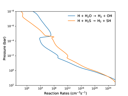
Figure 27: The rates of reactions that are key to recycle H back to H2, in the GJ 436b model including sulfur kinetics with $T_{\textrm{int}}$ = 400 K and weak vertical mixing (corresponding to the bottom right panel of Figure 25).

4.3.4 Sensitivity to S_x Polymerization

Since the growth from S2 to larger sulfur allotropes is suppressed in our GJ 436b model, we perform a sensitivity test to see if S_x beyond S2 can be produced with faster polysulfur recombination rates. The three-body recombination reactions that interconvert S2–S4–S8 are the main polymerization steps. We follow Zahnle et al. (2016) and raise the rate of S4 recombination by 10 and that of S8 recombination by 100 for a faster polysulfur forming test. We find the abundances of S4 and S8 remain low and almost unchanged. We confirm that the stratosphere of GJ 436b is too warm for elemental sulfur to grow beyond S2 into fair quantities, even after taken into account the uncertainties in the sulfur polymerization rates.

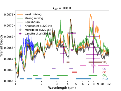
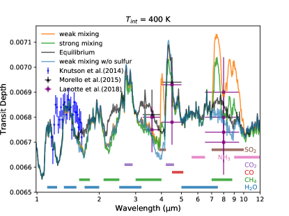
Figure 28: Synthetic transmission spectra computed for our GJ 436b model assuming $T_{\textrm{int}}$ = 100 K (top) and 400 K (bottom) with weak and strong vertical mixing. The model without sulfur chemistry (for $T_{\textrm{int}}$ = 400 K and weak vertical mixing) is also plotted for comparison. The HST/WFC3 points from Knutson et al. (2014) have been shifted down by 200 ppm, following Lothringer et al. (2018). The wavebands of main molecular absorption are indicated.

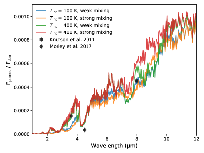
Figure 29: Synthetic emission spectra computed for our GJ 436b models including sulfur chemistry, in comparison with Spitzer secondary-eclipse data.

4.3.5 Transmission and Emission Spectra

The observational indication in transmission spectroscopy of varying vertical mixing and internal heating for GJ 436b is shown in Figure 28. The early analysis of Spitzer data (Knutson et al., 2011) has shown inter-epoch variability, which is reduced in the investigation of Lanotte et al. (2014); Morello et al. (2015). Methane absorption at 2.1-2.5 and 3-4 $\mu$m and sulfur dioxide absorption at 7-10 $\mu$m are the most promising diagnostic features. For $T_{\textrm{int}}$ = 100 K, vertical mixing leads to higher CH4 abundance and the strong mixing scenario can be marginally ruled out by the Spitzer 3.6-$\mu$m data. For $T_{\textrm{int}}$ = 400 K, vertical mixing conversely reduces CH4 abundances, confirmed with previous work by Agúndez et al. (2014) and Morley et al. (2017). The 3.6 and 4.5 $\mu$m Spitzer data are consistent with our models under weak/strong vertical mixing or in chemical equilibrium. While CH4 is not sensitive to the strength of vertical mixing at high internal heating scenario, SO2 shows strong dependence on mixing processes and is favored in our weak mixing scenario, which can potentially be detectable by JWST/MIRI. In addition, S2 is more favored with strong vertical mixing and provides strong absorption features in the UV.

Figure 29 shows the synthetic emission spectra for GJ 436b compared to Spitzer observations. While the 3.6 $\mu$m data prefers the $T_{\textrm{int}}$ = 400 K models, $T_{\textrm{int}}$ = 100 K models are favored by the 8 $\mu$m data. On the other hand, the already large column abundance of CO makes the thermal emission at 4.5 $\mu$m insensitive to internal heating or vertical mixing. The models somewhat overpredict the flux at 4.5 $\mu$m, as in the previous study (Morley et al., 2017)

We conclude that our models demonstrate and confirm that the combination of moderately high ($\gtrsim$ 100 times) solar metallicity and internal heating can explain the low CH4/CO ratio loosely constrained by the Spitzer 3.6 and 4.5 $\mu$m observations, regardless of the strength of mixing. Sulfur species do not quench in the deep region like CH4 or NH3 but closely associate with photolysis and mixing processes in the upper stratosphere. The independence from the thermal property of the interior makes sulfur chemistry a complementary avenue for characterizing GJ 436b, in conjunction with the long-standing quest for constraining CH4/CO.

4.4 51 Eridani b

51 Eridani b (51 Eri b) is a young Jupiter-mass giant around an F-type star at a wide orbit. Unlike irradiated hot Jupiters, the residual heat from the formation predominates over the stellar flux. In the discovery work, Macintosh et al. (2015) suggest 51 Eri b has an effective temperature 550 – 750 K with vertically quenched CH4 and CO. Water vapor should not condense owing to its heat at depth, in contrast to our colder Jupiter. The combination of the hot-interior and photochemically-active stratosphere makes 51 Eri b a unique testbed for atmospheric chemistry, as explored by Zahnle et al. (2016); Moses et al. (2016).

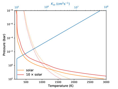
Figure 30: The temperature-pressure and eddy diffusion ($K_{\textrm{zz}}$) profiles for 51 Eri b, assuming solar and 10 times solar metallicity. The [CH4]/[CO] = 1 equilibrium transition curves corresponding to two metallicities are shown by the dotted curves.

4.4.1 Model Setup

We adopt $T_{\textrm{eff}}$ = 760 K as suggested by the retrieval work of Samland et al. (2017) for calculating the temperature profile of 51 Eri b (although we find little difference between setting $T_{\textrm{eff}}$ = 760 K and $T_{\textrm{eff}}$ = 700 K as assumed in previous work (Moses et al., 2016; Zahnle et al., 2016)). Samland et al. (2017) also derive a 10 times super-solar metallicity based on the K-band emission. To explore the effects of metallicity, we construct one temperature profile with solar metallicity and one with 10 times solar metallicity. The resulting P-T profiles are shown in Figure 30. We did not include a thermosphere as Moses et al. (2016) have added an arbitrary 1000 K inversion layer above 1 $\mu$bar but found little effects on the chemistry. The eddy diffusion takes the same form by Equation (29), with the radiative-convective transition P${}_{\textrm{tran}}$ and $K_{\textrm{deep}}$ set to 0.1 bar and 10⁵ cm²s^-1, respectively.

The stellar UV flux of 51 Eridani is assembled from various sources. The observations from the International Ultraviolet Explorer (IUE) covers the wavelength range between 115 and 198 nm. The EUV flux ($\lambda<$ 115 nm) is adopted from the synthetic spectrum of HR 8799 (Sanz-Forcada et al., 2011), following Moses et al. (2016). For wavelengths greater than 198 nm, we use a theoretical stellar spectrum with a close temperature from ATLAS9 Model Atmosphere Database by BOSZ stellar atmosphere model (Bohlin et al., 2017), assuming $T_{\textrm{eff}}$ = 7250 K, log(g) = 4, log[Fe/H] = 0, radius = 1.45 M_⊙. The stellar irradiation received by the planet in our 51 Eridani model is stronger by about 50 $\%$ than previous work, since the orbit has been updated from 13-14 AU to 11.1 AU according to De Rosa et al. (2020).

4.4.2 Disequilibrium Chemistry Compared with Previous Work

Zahnle et al. (2016) investigate sulfur hazes in the atmosphere of 51 Eri b. Moses et al. (2016) use an extensive N-C-H-O chemical network ($\sim$ 1650 reactions), which include more complex hydrocarbons, to study the quenching and photochemical effects. The mixing ratios of the main species in our 51 Eri b model for solar and 10 times solar metallicity are displayed in the top left panel of Figure 31. The main C, H, N, O chemical species in our model are overall consistent with both Zahnle et al. (2016) and Moses et al. (2016), which we summarize in the following paragraph.

The top row of Figure 31 shows how disequilibrium processes control the composition distribution. First, CH4-CO conversion is quenched at about 1 bar thus CO predominates over CH4. Likewise, N2 is the predominant nitrogen bearing species over NH3. Second, without the fast recycling mechanism like that on a hot Jupiter, strong photolysis of water makes the upper atmosphere oxidizing and produces considerable CO2 and O2. Third, C2H2 and HCN are photochemically generated in the upper atmosphere, similar to hot Jupiters. While C6H6 is produced to about 10 ppb level in Moses et al. (2016), C6H6 is greatly reduced in our model including sulfur, as seen for GJ 436b.

The most outstanding difference between Zahnle et al. (2016) and our model in terms of sulfur chemistry is that S8 reaches condensable level in our atmosphere. Although produced at about the same level, S8 is close to saturation but does not condense in the nominal model of Zahnle et al. (2016). Since we adopt the same saturation vapor pressure of sulfur allotropes (Lyons, 2008) as Zahnle et al. (2016), the different condensation behavior should be due to a warmer upper stratosphere in Zahnle et al. (2016). Zahnle et al. (2016) indeed noted that S8 would condense if the temperature were just a few degrees lower.

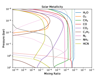
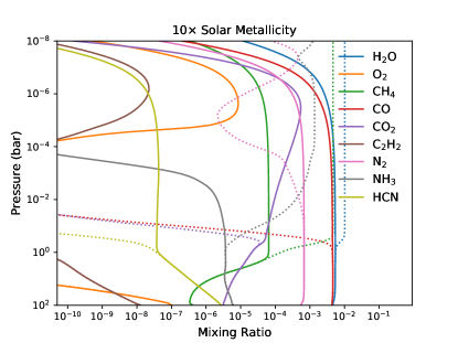
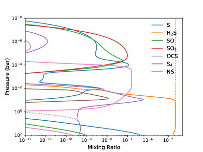
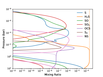
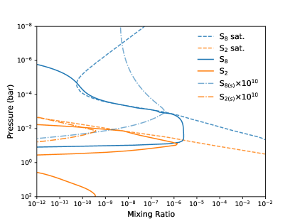
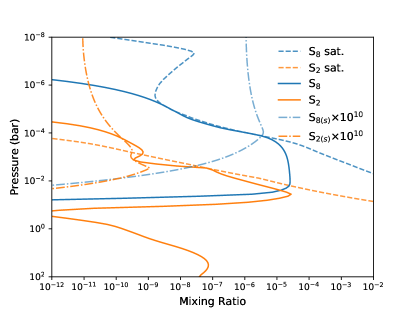
Figure 31: The computed abundance profiles of 51 Eri b, assuming solar (left panels) and 10 times solar (right panels) metallicity. The top row presents the main species, with equilibrium profiles shown in dotted lines. The middle row shows the main sulfur species and the bottom has S2/S8 vapor (solid), S2/S8 condensate particles (dashed-dotted), and the saturation mixing ratios of S2/S8 (dotted). The particles are plotted in the ratio of the number density of particles to the total number density of gas molecules and multiplied by 10¹⁰.

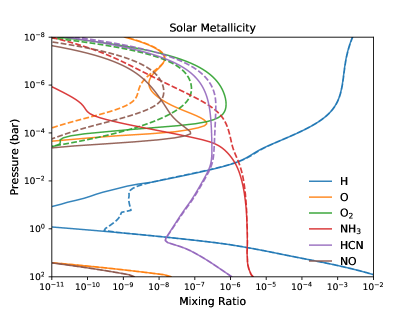
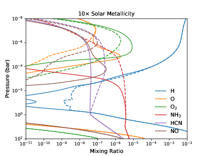
Figure 32: The abundances of several main species that show differences from models including sulfur kinetics (solid) and without sulfur kinetics (dashed) for 51 Eri b.

4.4.3 Effects of Super-Solar Metallicity

The left and right columns of Figure 31 compare the results of solar and 10 times solar metallicity. The model with 10 times solar metallicity has slightly hotter troposphere (Figure 30) which favored CO over CH4. Although the equilibrium abundance of CH4 in the stratosphere is increased in the 10 $\times$ solar metallicity model, CH4 is in fact decreased with a lower CH4/CO ratio at the quench level. In the end, the 10 $\times$ solar metallicity model shows higher CO, CO2, H2O and lower CH4 abundances, which in turn reduces other hydrocarbons as well. The mixing ratio of CO2 exceeds CH4 for 10 $\times$ solar metallicity and can reach $\sim$ 0.1$\%$ in the upper atmosphere. The production of O2 also raises with metallicity following the increase of water.

4.4.4 Effects of Sulfur

Compared to HD 189733b and GJ 436b, H2S can only remain stable against hydrogen abstraction (30) at higher pressure about 0.05 bar. The reverse rate of (30) significantly drops in the cooler stratosphere of 51 Eri b and prohibits the reformation of H2S. The active SH radical produced by H2S leads to a rich variety of sulfur species, as illustrated in the middle row of Figure 31. Compared to Zahnle et al. (2016), our model exhibits a more oxidized upper stratosphere due to stronger UV irradiaion from the closer orbit in our setting (11.1 AU compared to 13.2 AU). Nonetheless, both models predict efficient polymerization forming great abundance of S8. Since S8 is the end pool of sulfur chain reactions, we find the condensation of S8 does not affect other sulfur species. Elemental S is still the leading sulfur species above the S8 condensing layers until being oxidized into SO and SO2 in the upper stratosphere.

The equilibrium abundance of H2S scales with metallicity, which leads to more production of S8 vapor as metallicity increased. The 10 times solar metallicity model has slightly warmer temperature which allows higher saturation pressure of sulfur as well. In the end, both the gas and condensates of S2 and S8 increase with metallicity.

The effects of coupling to sulfur on other species are highlighted in Figure 32. The most remarkable feature is the enhanced oxygen abundances in the upper atmosphere with sulfur. In the absence of sulfur, atomic O can be released from H2O with the aid of CO2:

$$\begin{aligned} \ce{H2O&->[h\nu]OH+H}\\ \ce{CO+OH&->CO2+H}\\ \ce{CO2&->[h\nu]CO+O}\\ \vglue 5.0pt\cr\hline\cr\vglue 5.0pt\cr\mbox{net}:\ce{H2O&->[2h\nu]2H+O}.\end{aligned}$$ (33)

While sulfur is present, SO and SO2 dissociate more than CO2 around Ly-$\alpha$ and provide a faster channel to liberate O from H2O:

$$\begin{aligned} \ce{H2O&->[h\nu]OH+H}\\ \ce{SO+OH&->SO2+H}\\ \ce{SO2&->[h\nu]SO+O}\\ \vglue 5.0pt\cr\hline\cr\vglue 5.0pt\cr\mbox{net}:\ce{H2O&->[2h\nu]2H+O}.\end{aligned}$$ (34)

or

$$\begin{aligned} \ce{H2O&->[h\nu]OH+H}\\ \ce{S+OH&->SO+H}\\ \ce{SO&->[h\nu]S+O}\\ \vglue 5.0pt\cr\hline\cr\vglue 5.0pt\cr\mbox{net}:\ce{H2O&->[2h\nu]2H+O}.\end{aligned}$$ (35)

The excess atomic O readily reacts with OH to form O2. This enhanced oxidized region along with NS accelerates the oxidization of NH3, via the same pathway (32) but more pronounced than that on GJ 436b. On the other hand, CH4 is unaffected because the intermediates HCS and CS are deficient in the colder stratosphere of 51 Eri b. Lastly, the coupling to H2S also helps atomic H recycle back to H2 faster, as seen on GJ 436b.

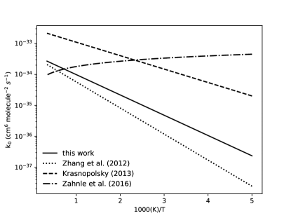
Figure 33: The low-pressure limit rate coefficient of S + CO -¿[M] OCS estimated in this work (37), compared to those in the literature.

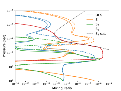
Figure 34: Main sulfur species from our nominal model with solar metallicity (solid) compared to those adopting the faster rate of (36) from Zahnle et al. (2016) (dashed).

4.4.5 sensitivity to OCS recombination

The fate of elemental S after being released from H2S is critical in sulfur kinetics. Several reactions potentially control whether S proceeds to chain formation into larger polysulfur (S_x), forming OCS, or being oxidized to SO, SO2. To address the effects of kinetics uncertainties, Zahnle et al. (2016) explore the sensitivity to H2S recombination and S_x polymerization. The authors found a faster H2S recombination counteracts the destruction of H2S and reduces the production of S8, while their results are not sensitive to the polymerizing rates of forming S4 and S8 within the tested ranges. We have tested the polymerization rates for GJ 436b and confirmed its general insensitivity to S8 formation. For 51 Eri b, we recognize that the recombination of OCS

$$\ce{S+CO->[\textrm{M}]OCS}$$ (36)

could be important in determining the oxidizing rate of sulfur. The rate coefficient of Reaction (36) has in fact not been measured. Only the reverse step of (36), the dissociation of OCS, has available data at high temperatures. Recently, Ranjan et al. (2020) has also identified this reaction to modestly alter the CO abundance in a CO2-N2 atmosphere and advocate laboratory investigation. Here, we will explain how the rate coefficient of Reaction (36) is estimated in our nominal model and then explore the sensitivity to the uncertainty for 51 Eri b.

Reaction (36) is a spin-forbidden reaction and usually many orders of magnitude slower than a typical three-body reaction. Since the measured high-temperature dissociation reaction has a high activation energy, extrapolating the dissociation reaction (the reversal of (36)) to low temperatures will result in unrealistically rates. Instead, we estimate the activation energy from the well-studied analogous reaction, O + CO -¿[M] CO2. The pre-exponential factor is then determined by matching the reverse of dissociation reaction at 2000 K from Oya et al. (1994). The low-pressure limit rate of (36) we estimate is

$$k_{\textrm{0}}=4.47\times 10^{-34}\textrm{exp}(-1510/T).$$ (37)

We compare the rate coefficient (37) with those assumed in Zahnle et al. (2016) and Venus literature (Zhang et al., 2012; Krasnopolsky, 2013) in Figure 33. The reaction rates show diverse values especially toward lower temperatures, the relevant temperature range for the stratosphere of 51 Eri b. Albeit the rate discrepancy in each model, the rate constants in Zhang et al. (2012), Krasnopolsky (2013) and this work exhibit consistent temperature dependence from 1000 K to 200 K, whereas that in Zahnle et al. (2016) has suprisingly almost no temperature dependence. Since rate constant of (36) from Zahnle et al. (2016) is the most different from the literature and yields fastest OCS forming rate, we will use the rate from Zahnle et al. (2016) as the upper limit to test the sensitivity.

We run our nominal model with solar metallicity but adopt the rate constant of (36) from Zahnle et al. (2016). The effects of faster OCS recombination are illustrated in Figure 34. With the OCS recombination rate from Zahnle et al. (2016), OCS mixing ratio is significantly increased above 0.1 bar. S8 is slightly reduced but remains the major sulfur carrier between 10^-2 and 10^-4 bar, consistent with the model results in Zahnle et al. (2016). The abundance of S and S2 are subsequently affected by more ample OCS photodissociation but that of S8 remains the same as set by condensation. Given these differences, we reiterate further investigation to pin down the reaction rate of OCS recombination.

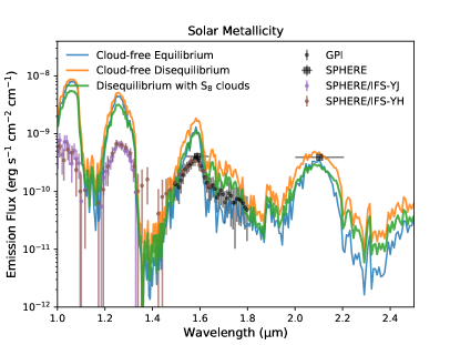
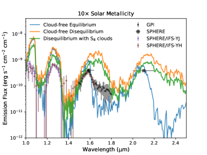
Figure 35: Synthetic emission spectra of 51 Eri b produced from equilibrium abundances, disequilibrium abundances, and with S8 condensate layer. Data points show GPI observations from Macintosh et al. (2015) and SPHERE observations from Samland et al. (2017).

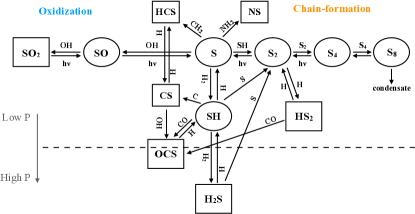
Figure 36: A Schematic diagram illustrating the main pathways for sulfur kinetics in an H2-dominated atmosphere. The dashed line represents the transition from the lower region where sulfur is predominantly locked in H2S to the upper region where H2S is subject to dissociation. Rectangles indicate stable species whereas ellipses indicate active radical or intermediate species.

4.4.6 Emission Spectra

Figure 35 demonstrates the effects of disequilibrium chemistry and S8 clouds on the planetary emission spectra. For both metallicities, quenched CH4 and H2O have lower abundances than equilibrium, leading to higher emission in the H and J bands from the deeper region. The 10 times solar metallicity further reduces CH4 and prompts the flux at 1.6 - 1.8 $\mu$m. We assume 1 $\mu$m particle size for S8 condensates, which scatter strongly and reduce the emission in this wavelength range. However, using the higher effective temperature and metallicity from Samland et al. (2017), our models generate emission that are too high in the H and J bands and fail to reproduce the observed spectra. We conclude that either $T_{\textrm{eff}}$ is lower than that determined by Samland et al. (2017) and/or additional cloud layers (e.g. Moses et al., 2016) is required to match the lower observed emission.

4.5 Sulfur Mechanism

Figure 36 summerizes the important pathways for sulfur species in the irradiated H2-dominated atmospheres we explored in this section. H2S is the dominant molecule, which is thermochemically stable for a wide range of temperatures in the lower atmosphere followed by OCS. The photochemistry of sulfur is initiated from SH and S produced by H2S dissociation, leading to multiple channels including chain formation and oxidization depending on the atmospheric condition. Sulfur chain formation is highly temperature sensitive where S2 is favored about 600 - 800 K and S8 can only form below $\sim$ 500 K (e.g. the stratosphere of 51 Eri b). When OH is sufficiently produced by H2O photolysis, S will most likely be oxidized into SO and SO2 in the upper atmosphere. S also participates in accelerating CH4 and NH3 destruction via the coupling to CH2 or NH2, as seen in our HD 189733b and GJ 436b models.

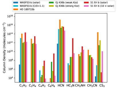
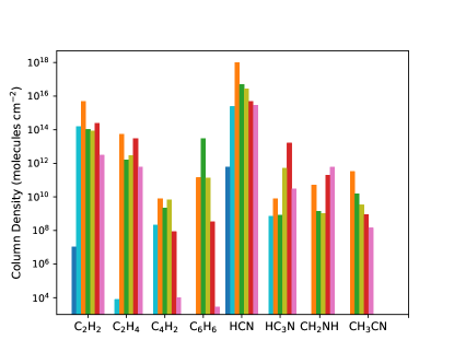
Figure 37: The column number densities (molecules cm^-2) above 1 mbar of haze precursors for the simulated atmospheres in Section 4, including sulfur (left) and without sulfur (right). Some molecule abundances are negligible and not shown for WASP-33b. For GJ 436b, the models with T${}_{\textrm{int}}$ = 400 K and weak/strong vertical mixing are used.

4.6 Trends of Photochemical Hazy Precursors

Figure 37 summarizes the column densities of haze precursors above 1 mbar for the simulated atmospheres in Section 4. Across the various irradiated H2-atmospheres we explored, we find HCN consistently to be the most prevailing precursor. This is not surprising as HCN is a robust photochemical product of CH4 and NH3 and also recently been detected on HD 209458b (Giacobbe et al., 2021). Nonetheless, it does not necessarily imply HCN will lead to complex nitriles formation, since HCN is not the limiting factor as we discussed in Section 2.8. A more careful assessment at high temperatures is required before extrapolating the haze-forming mechanism below 200 K on Titan. We observe a general increasing trend with decreasing temperature for the more indicative nitrile precursors HC3N but opposite for CH3CN. The same trend is seen for the hydrocarbon precursors C4H2 and C6H6.

Only HCN and C2H2 can reach appreciable levels on WASP-33b, even as photochemical hazes are not expected on WASP-33b. For GJ 436b, most of the precursors are not too sensitive to eddy diffusion. For 51 Eri b, almost all precursors are reduced with increasing metallicity, except for CS2 since it contains no H. In fact, CS2 is most favored on HD 189733b, which suggests sulfur-containing hazes in the hot Jupiter condition as carbon and sulfur can couple closely. In addition to sulfur condensates, 51 Eri b might also be covered by nitrile-type hazes according to the precursor distribution.

5 Discussion

5.1 High-Temperature UV Cross Sections

We have implemented layer-by-layer UV cross sections according to the temperature at each atmospheric level in VULCAN. Due to the sparsely available data, we did not perform systematic study in this work. Nonetheless, we have gained some insights through the case studies in Section 4.

We found the effects of temperature dependence for H2O is mostly negligible in a H2-dominated atmosphere. However, this is solely based on the limited wavelength-range measurements we assembled. For the high-temperature ($T>$ 1000 K) cross sections, only wavelengths longer than about 190 nm are included (Figure 38). The high-temperature cross sections in the FUV could have larger effects.

We confirm the analysis in Venot et al. (2013) that although the CO2 abundance is not directly influenced by the temperature dependence of CO2 photolysis, the shielding effects can impact other species. As CO2 absorb more strongly with increasing temperature, the UV photosphere is lifted to lower pressure. The production of radicals, such as H and OH, is reduced and subsequently alters other species. However, we also find that the shielding effects of CO2 are completely shadowed when sulfur species are included (e.g. see the right panel of Figure 18). The temperature dependence of CO2 photolysis should be more amplified in CO2-dominated atmospheres.

5.2 Implication of Ionization

Ions are not included in this work. We are working on including ionchemistry in the next update of VULCAN. Photoionization is known to be critical in initiating the haze formation (Wong et al., 2003; Krasnopolsky, 2009; Plessis et al., 2012; Lavvas et al., 2013). Even thermoionization can be important for ultra hot Jupiters. In our study about WASP-33b, atomic Ti and V in the upper atmosphere are expected to be partly ionized and contribute to free electrons. Since Ti has an ionization threshold of 180 nm, compared to about 240 nm for Na, the effects of photoionization on Ti and V should be similar and probably smaller than those on the alkali atoms, as investigated in Lavvas & Koskinen (2017). An important outcome of photoionization is that the increased electrons can lead to more hydrogen anions (H-) than predicted by thermal equilibrium, which are found to be important opacity sources in some hot Jupiters atmospheres (Lewis et al., 2020). In terms of sulfur chemistry, several sulfur species have relatively lower-energy threshold of ionization and can be subject to photoionization. For example, atomic S starts to ionize from Lyman-$\alpha$. Since S is likely the dominant sulfur species in the hot Jupiter’s stratosphere (Section 4.2.2), S can be photoionized and ramify into various organic molecules through ion-exchange reactions.

5.3 More Intriguing Questions about Sulfur

In Section 4, we find the coupling to sulfur chemistry impacts the core C-H-N-O kinetics in several ways for H2-dominated atmospheres. The coupling effects essentially depend on if the sulfur-containing intermediates are active, which is not well-understood in general as it can vary with atmospheric conditions such as temperature and bulk compositions. Gersen et al. (2017) find that CH3S and CH3SH provide more efficient pathways for methane oxidization in the combustion (oxidizing) environment. He et al. (2020) also observe the photochemical formation of CH3S and CH3SH in a CO2-rich gas mixture in the experiments. Although we have included reactions involving CH3S and CH3SH in our sulfur mechanism, they are not identified to be important in the pathway analysis for all of the H2-atmospheres we investigated. The chemical role of CH3SH is worth further study in the broad context of biologically produced sulfur.

The temperature profiles are fixed without considering the radiative feedback in this whole work. The radiative effects might be more prominent in the presence of sulfur, such as the absorption of SH and S2 in the optical and NUV. 51 Eri b or other directly imaged planets with a relatively cold stratosphere ($\lesssim$ 500 K) and under sufficient UV irradiation sit in the sweet spot for testing the radiative feedback on sulfur condensates.

6 Summary

In this paper, we present a thorough theoretical framework of the updated photochemical code VULCAN. We validate our models for the atmospheres of hot Jupiters, Jupiter, and modern Earth and carry out comparative study on representative cases of extrasolar giant planets: WASP-33b, HD 189733b, GJ 436b, and 51 Eridani b. The highlights of our results are:

• We have carefully validated the model of HD 189733b. The updated methanol scheme in Venot et al. (2020) is found to bring the quenching behavor of methane close to Moses et al. (2011) and VULCAN. We pointed out the photochemical source plays a non trivial part in the model differences between Moses et al. (2011), Venot et al. (2012), and VULCAN.

• We demonstrate advection transport in the downdraft can qualitatively explain the deep ammonia distribution in Jupiter, which can not be explained by eddy diffusion alone.

• The implementation of surface boundary conditions and condensation in an oxygen-rich atmosphere is validated in the present-day Earth model. A general oxidation timescale analysis is provided for assessing the chemical lifetime of biosignature gases.

• The atmosphere of WASP-33b is not affected by vertical quenching but consisted of an upper photolytic region and a thermochemical equilibrium region below. For GJ 436b, we find NH3 insensitive to vertical mixing and the sulfur species governed by photolysis and mixing in the upper stratosphere are independent of the deep thermal structure, which can be complementary to the CH4/CO metric for breaking degeneracies. The quenched CO always predominates over CH4 on 51 Eri b and sulfur aerosols (chiefly S8) condense out in the stratosphere.

• We find the coupling to sulfur chemistry impact C-H-N-O kinetics. Sulfur can provide catalytic paths to destroy CH4 and NH3 and generally lower the hydrocarbon abundances. H2S makes H recycled back to H2 faster on the cooler GJ 436b and 51 Eri b. The dissociation of SO and SO2 also make the upper atmosphere of 51 Eri b more oxidizing.

• We suggest including several photochemical haze precursors such as C6H6 and HC3N, which are more indicative than the commonly considered HCN and C2H2. We observe a general increasing trend with decreasing temperature for C4H2, C6H6, and HC3N but opposite for CH3CN.

Model availability

The results in this work are produced by version 2.0 of VULCAN (https://github.com/exoclime/VULCAN/releases/tag/v2.0). In addition to the public code, the configuration files used for the models in Section 3 are available on https://github.com/exoclime/VULCAN and the main model output in Section 3 and Section 4 can be found in the supplementary material.

Software: Python; Numpy (van der Walt et al., 2011); Scipy (Oliphant, 2007); Matplotlib (Hunter, 2007)

Appendix A Molecular diffusion and thermal diffusion factor

For H2-based atmospheres, we take

$$D_{\ce{H2}-\ce{CH4}}=2.2965\times 10^{17}T^{0.765}/N$$ (A1)

from Marrero & Mason (1972) as the reference and scale the molecular diffusion coefficient of H2 with other species according to Equation (3). The thermal diffusion factor for H and He are approximately $\alpha_{\ce{H}}$ $\approx$ -0.1 and $\alpha_{\ce{He}}$ $\approx$ 0.145 (Moses et al., 2000). We assume $\alpha_{i}$ = -0.25 for the rest of species based on rigid sphere approximation (Banks & Kockarts, 1973).

For N2-based atmospheres, we take

$$D_{\ce{N2}-\ce{CH4}}=7.34\times 10^{16}T^{0.75}/N$$ (A2)

from Banks & Kockarts (1973) as the reference and scale the molecular diffusion coefficient of N2 with other species according to Equation (3). The thermal diffusion factor of Ar is $\alpha_{\ce{Ar}}$ $\approx$ 0.17 and $\alpha_{i}$ = -0.25 for the rest species.

For CO2-based atmospheres, we take

$$D_{\ce{CO2}-\ce{H2}}=7.51\times 10^{16}T^{0.759}/N$$ (A3)

from Banks & Kockarts (1973) as the reference and scale the molecular diffusion coefficient of CO2 with other species according to Equation (3). The thermal diffusion factor of Ar is $\alpha_{\ce{Ar}}$ $\approx$ 0.17 and $\alpha_{i}$ = -0.25 for the rest species.

Appendix B Resolution Errors of Photolysis Rates

Table 4: Errors from Low Spectral Resolution

Bin (nm)	Stellar Flux (in $\%$)	$\Delta$ J${}_{\ce{H2}}$	$\Delta$ J${}_{\ce{H2O}}$
0.2	0	0.0004	0.003
0.5	0.08	0.18	1.13
1	0.08	0.44	0.87
10	2.65	0.22	0.87

Equation (11) is numerically computed in the form of finite sum. The wavelength grid in the code needs to properly resolve the line structures in the stellar flux and cross sections. This is especially important in the XUV where there are more fine structures from the band transition (Rimmer & Helling, 2016).

We demonstrate the errors of computing Equation (11) with the GJ 436b model in Section 4.3. The effects are emphasized with its host M-star showing more emission lines. Figure 39 shows the stellar flux overplotted with the UV cross sections of H2 and H2O. The stellar flux is adopted from the MUSCLES survey with a constant 0.1 nm resolution and the UV cross sections from the Lieden database have the same resolution of 0.1 nm. Therefore, we consider constant resolution of 0.1 nm as the reference for this test. The resolution for computing Equation (11) is varied from 0.2 nm to 10 nm, where the trapezoidal rule is applied for the integral. The errors with respect to summing-up the total stellar flux and the resultant photolysis rate of H2 and H2O at the top of atmosphere (10^-8 bar) are summerized in Table 4. Starting from the bin size of 0.5 nm, which is five times the native resolution of the flux and cross section data, the errors become comparable to the absolute value of the photolysis rate. The errors do not behave linearly with the bin size since the overestimate from the peak can offset the underestimate from the trough. The test shows the importance of using matching spectral resolution to attain accurate photolysis rates.

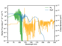
Figure 39: The stellar UV flux of GJ 436 and cross sections of H2 and H2O, showing the native resolution 0.1 nm adopted in the model.

Table 5: List of forward reactions (backward reactions with even indexes are reversed numerically with thermodynamic data) and rate coefficients (cm³ s^-1 for bimolecular reactions and s^-1 for k₀) of titanium and vanadium species. $E_{a}$ est. means the activation energy is estimated by the enthalpy difference as described in Section 2.7.

Reaction	Rate Coefficient	Reference
TiO + O -¿ Ti + O2	5.42 $\times 10^{-13}$ $\exp(-20794/T)$	$E_{a}$ est. with $A$ from matching NIST 1994LIA/MIT (at room temperature)
TiO + N -¿ Ti + NO	4.76 $\times 10^{-12}$ $\exp(-4772/T)$	$E_{a}$ est. with $A$ from matching NIST1993CLE/HON (at room temperature)
TiO + N2 -¿ Ti + N2O	5.9 $\times 10^{-12}$ $\exp(-62193/T)$	$E_{a}$ est. with $A$ from matching NIST 1994LIA/MIT (at room temperature)
TiO + H -¿ Ti + OH	2.0 $\times 10^{-10}$ $\exp(-28418/T)$	$E_{a}$ est. with $A$ based on FeO + H -¿ Fe + OH from Rumminger et al. (1999)
TiO + H2 -¿ Ti + H2O	2.0 $\times 10^{-11}$ $\exp(-21270/T)$	$E_{a}$ est. with $A$ based on FeO + H2 -¿ Fe + OH from Decin et al. (2018)
Ti + CO2 -¿ TiO + CO	7.01 $\times 10^{-11}$ $\exp(-1790/T)$	NIST 1993CAM/MCC7942-7946
TiO2 + H -¿ TiO + OH	$1.0\times 10^{-10}\exp(-19500/T)$	$E_{a}$ est. with $A$ based on FeO2 + H -¿ FeO + OH from Rumminger et al. (1999)
TiO2 + O -¿ TiO + O2	$1.0\times 10^{-10}\exp(-11877/T)$	$E_{a}$ est.
TiO2 + CO -¿ TiO + CO2	$1.0\times 10^{-10}\exp(-9160/T)$	$E_{a}$ est. with $A$ based on FeO2 + O -¿ FeO + O2 from Rumminger et al. (1999)
TiH + H -¿ Ti + H2	8.3 $\times 10^{-11}$	Est. from FeH + H -¿ Fe + H2 (Rumminger et al., 1999)
TiH + O -¿ Ti + OH	1.66 $\times 10^{-10}$	Est. from FeH + O -¿ Fe + OH (Rumminger et al., 1999)
TiH + CH3 -¿ Ti + CH4	1.0 $\times 10^{-10}$	Est. from FeH + CH3 -¿ Fe + CH4 (Rumminger et al., 1999)
TiC + H -¿ Ti + CH	$1.0\times 10^{-10}\exp(-20109/T)$	$E_{a}$ est.
Ti + CO -¿ TiC + O	$8.0\times 10^{-10}\exp(-68842/T)$	$E_{a}$ est.
Ti + CN -¿ TiC + N	$5.0\times 10^{-10}\exp(-29543/T)$	$E_{a}$ est.
Ti + NO -¿ TiN + O	$5.0\times 10^{-11}\exp(-19706/T)$	$E_{a}$ est. with $A$ from matching Campbell & McClean (1993)
TiN + H -¿ Ti + NH	$10^{-10}\exp(-15655/T)$	$E_{a}$ est.
VO + O -¿ V + O2	$6.19\times 10^{-12}$ $\exp(-14763/T)$	$E_{a}$ est. with $A$ from matching NIST 1990RIT/WEI (at room temperature)
V + N2O -¿ VO + N2	$4.7\times 10^{-11}$ $\exp(-1299/T)$	NIST 2000CAM/KOL
VO + H -¿ V + OH	$1.66\times 10^{-10}$ $\exp(-22386/T)$	$E_{a}$ est. with $A$ based on FeO + H -¿ Fe + OH from Rumminger et al. (1999)
VO + H2 -¿ V + H2O	$1.0\times 10^{-11}$ $\exp(-15239/T)$	$E_{a}$ est. with $A$ based on FeO + H2 -¿ Fe + H2O from Decin et al. (2018)
TiO2 -¿[M] Ti + O2	$k_{0}$ = $1.38\times T^{-1.8}$ $\exp(-94079/T)$ $k_{\infty}$ = $2\times 10^{17}$ $T^{-0.91}$ $\exp(-94079/T)$	$E_{a}$ est. $A$ based on FeO2 -¿[M] Fe + O2 from Rumminger et al. (1999)
TiO -¿[M] Ti + O	$k_{0}$ = $1.38\times T^{-1.8}$ $\exp(-82202/T)$ $k_{\infty}$ = $2\times 10^{17}$ $T^{-0.91}$ $\exp(-76171/T)$	$E_{a}$ est. $A$ based on FeO -¿[M] Fe + O from Rumminger et al. (1999)
VO -¿[M] V + O	$k_{0}$ = $1.38\times T^{-1.8}$ $\exp(-76171/T)$ $k_{\infty}$ = $2\times 10^{17}$ $T^{-0.91}$ $\exp(-76171/T)$	$E_{a}$ est. $A$ based on FeO -¿[M] Fe + O from Rumminger et al. (1999)

Table 6: Full List of Photolysis Reactions in VULCAN

Photolysis	Reaction	Threshold (nm)	Temp. Dependence (K)	Reference Cross Sections / Quantum Yields ($\lambda$ in nm)
H2O	-¿ H + OH	207	300, 423, 573, 1230, 1540, 1630, 1820, 2010, 2360	a, b, e / d, Stief et al. (1975); Slanger & Black (1982)
	-¿ H2 + O(^1D)
	-¿ O + H + H
CH4	-¿ CH3 + H	145	—	a / d ($\lambda$ $<$ 97.7), Gans et al. (2011) ($\lambda$ $\geq$ 118.2)
	-¿ ^1CH2 + H2
	-¿ ^1CH2 + H + H
	-¿ CH + H2 + H
CH3	-¿ CH + H2	220	—	a / Lavvas et al. (2008); Kassner & Stuhl (1994)
	-¿ CH2 + H
CH2	-¿ CH + H	275	—	a / a
CO	-¿ C + O	166	—	a, b/ a
H2	-¿ H + H	120	—	a / a
C2H2	-¿ C2H + H	217	—	a / a, Okabe (1983)
CO2	-¿ CO + O	202	150, 170, 195, 230, 300, 420, 500, 585, 700, 800, 1160	a, Venot et al. (2018) , e / b
	-¿ CO + O(^1D)
C2H4	-¿ C2H2 + H2	195	—	a / Lavvas et al. (2008) and the references in
	-¿ C2H2 + H + H
	-¿ C2H3 + H
C2H6	-¿ C2H4 + H2	165	—	a / b, Lias et al. (1970) (104 $<$ $\lambda$ $<$ 105)
	-¿ C2H4 + H + H
	-¿ C2H2 + H2 + H2
	-¿ CH4 + ^1CH2
	-¿ CH3 + CH3
C4H2	-¿ C2H2 + C2	197	—	a / Lavvas et al. (2008)
C6H6	-¿ C6H5 + H	206	—	a / Est. from Kislov et al. (2004)
	-¿ C3H3 + C3H3
OH	-¿ O + H	265	—	a / a, b ($\lambda$ $<$ 91)
HCO	-¿ H + CO	656	—	a / a
H2CO	-¿ H2 + CO	360	—	a / b ($\lambda$ $<$ 250), d
	-¿ H + HCO
CH3OH	-¿ CH3 + OH	220	—	a / b, Hagege et al. (1968)
	-¿ H2CO + H2
	-¿ CH3O + H
CH3CHO	-¿ CH4 + CO	350	—	a / b
	-¿ CH3 + HCO
N2	-¿ N + N	150	—	a ($\lambda$ $<$ 100), c ($\lambda$ $>$ 120) / a
NH3	-¿ NH2 + H	226	175, 300, 562	a / b
	-¿ NH + H + H
HCN	-¿ H + CN	179	—	a / Nuth & Glicker (1982)
NO	-¿ N + O	202		a / a
NO2	-¿ NO + O	398		b, Voigt et al. (2002) / b, d
NO3	-¿ NO2 + O	703	—	b / b, Sander et al. (2015)
	-¿ NO + O2
N2O	-¿ NO + O(^1D)	340	300, 714, 833, 1000, 1250, 1667, 2000	a,c (Zuev & Starikovskii, 1990)) / b
HNO2	-¿ NO + OH	591	—	b / b
HNO3	-¿ NO2 + OH	598	—	b / b
N2O5	-¿ NO3 + NO2	500	—	b / b (from here)
	-¿ NO3 + NO + O
N2H4	-¿ N2H3 + H	291	—	c (BiehlStuhl(1991) and Vaghjiani(1993) 296K 191-291n) / Lavvas et al. (2008)
O2	-¿ O + O	240	200, 250, 300, 873, 1073	a / b,d
	-¿ O + O(^1D)
O3	-¿ O2 + O	900	—	a / Matsumi(2002)
	-¿ O2 + O(^1D)
HO2	-¿ O + OH	275	—	a / a
H2O2	-¿ OH + OH	350	—	a / a
HNCO	-¿ NH + CO	354	—	b / b
	-¿ H + NCO
SH	-¿ S + H	345	300, 500, 750, 1000, 1250, 1500, 1750, 2000, 2250, 2500, 3000	a, Gorman et al. (2019) for $\lambda$ $\geq$ 314 nm / a
H2S	-¿ SH + H	238	423, 573, 773	a, e / a
SO	-¿ S + O	235	—	a / a
SO2	-¿ SO + O	220	—	a / a
	-¿ S + O2		—	a / a
S2	-¿ S + S	283	—	a / a
S4	-¿ S + S	575	—	a / a
OCS	-¿ CO + S	280	—	a / a
CS	-¿ C + S	160	—	a / a
CS2	-¿ CS + S	278	300, 423, 573, 773	a / a
CH3SH	-¿ CH3S + H	310	—	a / b
	-¿ CH3 + SH

a: Leiden Observatory database (Heays et al., 2017) b: PHIDRATES database (Huebner et al., 1992) c: MPI-Mainz UV/VIS Spectral Atlas (Keller-Rudek et al., 2013)) d: Sander et al. (2015) e: ExoMol database

Appendix C The Choice of Zenith Angle

A global or hemispheric average 1-D photochemical model requires specifying an effective zenith angle ($\overline{\theta}$) of the stellar beam to represent the planetary-mean actinic flux. The zenith angle of 48^∘ – 60^∘ has been used for the hemispheric average in various photochemical models (e.g. Moses et al. (2011); Hu et al. (2012)). For instance, a common choice in radiative transfer calculation is to take the flux-weighted cosine of the zenith angle (Cronin, 2014):

$$\overline{\mu_{\textrm{I}}}=\frac{\int_{0}^{2\pi}\int_{0}^{1}\mu F_{0}\mu d\mu d\phi}{\int_{0}^{2\pi}\int_{0}^{1}F_{0}\mu d\mu d\phi}$$ (C1)

where $\phi$ is the azimuth angle and $F_{0}$ is the stellar flux at the top of atmosphere. Equation (C1) yields $\overline{\mu_{\textrm{I}}}$ = 2/3 or $\overline{\theta_{\textrm{I}}}\approx$ 48^∘. For photochemistry calculation, actinic-flux-weighted cosine should be considered and Equation (C1) becomes

$$\overline{\mu_{\textrm{II}}}=\frac{\int_{0}^{1}\mu J_{0}d\mu}{\int_{0}^{1}J_{0}d\mu}$$ (C2)

where $J_{0}$ is the actinic flux at the top of atmosphere (i.e. total intensity) and the azimuth term is dropped. Equation (C2) now yields $\overline{\mu_{\textrm{II}}}$ = 1/2 or $\overline{\theta_{\textrm{II}}}$ = 60^∘.

Hu et al. (2012) discuss this choice of mean zenith angle by further considering the optical depth of the level where the hemispheric average of the attenuated actinic flux is evaluated, e.g., the authors find a mean zenith angle of 57^∘ and 48^∘ correspond to optical depth 0.1 and 1, respectively. We will revisit the discussion of Hu et al. (2012) but with a different approach here.

Instead of taking the average of $\mu$, we consider an effective zenith angle such that the resulting mean actinic flux matches the hemispheric-mean actinic flux, viz.

$$J_{0}\,\textrm{exp}(-\frac{\tau}{\overline{\mu}}) =\frac{\int_{0}^{1}J_{0}\,\textrm{exp}(-\frac{\tau}{\mu})d\mu}{\int_{0}^{1}d\mu}$$ (C3)

$$=J_{0}\int_{0}^{1}\textrm{exp}(-\frac{\tau}{\mu})d\mu.$$

Equation (C3) can be evaluated numerically at the given optical depth, as illustrated in Figure 40. We find that optical depth unity (i.e. where UV photons are mostly utilized for photochemistry) corresponds to $\overline{\theta}$ $\approx$ 58^∘. Note that the evaluation in Hu et al. (2012) is similar to Equation (C3) but weighted by $\mu$ within the integral, which is effectively the mean stellar flux instead of the actinic flux. Evaluating Equation (C3) at $\tau=1$, we find $\overline{\theta}$ $\approx$ 58^∘ for a dayside-average model. For a terminator-average model, the denominator in Equation (C3) is integrated from -1 to 1 and we have $\overline{\theta}$ $\approx$ 67^∘.

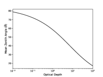
Figure 40: Dayside mean zenith angle for photochemical calculation as a function of optical depth from Equation (C3).

References

- Agúndez et al. (2014) Agúndez, M., Venot, O., Selsis, F., & Iro, N. 2014, ApJ, 781
- Allen et al. (1981) Allen, M., Yung, Y. L., & Waters, J. W. 1981, Journal of Geophysical Research: Space Physics, 86
- Arney (2019) Arney, G. N. 2019, The Astrophysical Journal, 873
- Atkinson et al. (1997) Atkinson, D. H., Ingersoll, A. P., & Seiff, A. 1997, Nature, 388
- Atreya et al. (2020) Atreya, S. K., Hofstadter, M. H., In, J. H., et al. 2020, Space Sci. Rev., 216
- Atreya et al. (2005) Atreya, S. K., Wong, A. S., Baines, K. H., Wong, M. H., & Owen, T. C. 2005, Planet. Space Sci., 53
- Ayres (2010) Ayres, T. R. 2010, ApJS, 187
- Banks & Kockarts (1973) Banks, P. M., & Kockarts, G. 1973, Aeronomy.
- Barkley et al. (2008) Barkley, M. P., Palmer, P. I., Boone, C. D., Bernath, P. F., & Suntharalingam, P. 2008, Geophysical Research Letters, 35
- Baxter et al. (2021) Baxter, C., Désert, J.-M., Tsai, S.-M., et al. 2021, arXiv e-prints, arXiv:2103.07185. https://arxiv.org/abs/2103.07185
- Birkby et al. (2013) Birkby, J. L., de Kok, R. J., Brogi, M., et al. 2013, Monthly Notices of the Royal Astronomical Society: Letters, 436
- Boechat-Roberty et al. (2004) Boechat-Roberty, H. M., Rocco, M. L. M., Lucas, C. A., & de Souza, G. G. B. 2004, Journal of Physics B: Atomic, Molecular and Optical Physics, 37
- Bohlin et al. (2017) Bohlin, R. C., Mészáros, S., Fleming, S. W., et al. 2017, AJ, 153
- Bolton et al. (2017) Bolton, S. J., Adriani, A., Adumitroaie, V., et al. 2017, Science (80-. )., 356
- Bordwell et al. (2018) Bordwell, B., Brown, B. P., & Oishi, J. S. 2018, The Astrophysical Journal, 854
- Bourrier et al. (2020) Bourrier, V., Wheatley, P. J., Lecavelier des Etangs, A., et al. 2020, MNRAS, 493
- Brasseur & Jacob (2017) Brasseur, G. P., & Jacob, D. J. 2017, Numerical Methods for Advection (Cambridge University Press), , p275–341
- Brogi et al. (2014) Brogi, M., de Kok, R. J., Birkby, J. L., Schwarz, H., & Snellen, I. A. G. 2014, A&A, 565
- Burke et al. (2016) Burke, U., Metcalfe, W. K., Burke, S. M., et al. 2016, Combustion and Flame, 165
- Burrows et al. (2005) Burrows, A., Dulick, M., Bauschlicher, C. W., et al. 2005, Astrophys. J., 624
- Butler et al. (2004) Butler, R. P., Vogt, S. S., Marcy, G. W., et al. 2004, The Astrophysical Journal, 617
- Campbell & McClean (1993) Campbell, M. L., & McClean, R. E. 1993, J. Phys. Chem., 97
- Capalbo et al. (2016) Capalbo, F. J., Bénilan, Y., Fray, N., et al. 2016, Icarus, 265
- Chachan et al. (2019) Chachan, Y., Knutson, H. A., Gao, P., et al. 2019, AJ, 158
- Chamberlain & Hunten (1987) Chamberlain, J. W., & Hunten, D. M. 1987, in International Geophysics, Vol. 36, Theory of Planetary Atmospheres, ed. J. W. Chamberlain & D. M. Hunten (Academic Press), 330 – 415
- Charnay et al. (2015) Charnay, B., Meadows, V., & Leconte, J. 2015, ApJ, 813
- Chauvin (2018) Chauvin, G. 2018, arXiv e-prints, arXiv:1810.02031. https://arxiv.org/abs/1810.02031
- Chestakov et al. (2005) Chestakov, D. A., Parker, D. H., & Baklanov, A. V. 2005, The Journal of Chemical Physics, 122
- Chiou et al. (1997) Chiou, E. W., McCormick, M. P., & Chu, W. P. 1997, Journal of Geophysical Research: Atmospheres, 102
- Cloutman (2000) Cloutman, L. 2000, Lawrence Livermore National Laboratory report, UCRL-ID-139893
- Cronin (2014) Cronin, T. W. 2014, J. Atmos. Sci., 71
- Crossfield (2015) Crossfield, I. J. M. 2015, Publications of the Astronomical Society of the Pacific, 127
- Davidson et al. (1989) Davidson, D. F., Chang, A. Y., & Hanson, R. K. 1989, Symposium (International) on Combustion, 22
- De Rosa et al. (2020) De Rosa, R. J., Nielsen, E. L., Wang, J. J., et al. 2020, AJ, 159
- Dean & Bozzelli (2000) Dean, A. M., & Bozzelli, J. W. 2000, Combustion chemistry of nitrogen (Springer), 125–341
- Dean et al. (1984) Dean, A. M., Chou, M.-S., & Stern, D. 1984, International Journal of Chemical Kinetics, 16
- Decin et al. (2018) Decin, L., Danilovich, T., Gobrecht, D., et al. 2018, Astrophys. J., 855
- Demory et al. (2007) Demory, B. O., Gillon, M., Barman, T., et al. 2007, A&A, 475
- Drossart et al. (1999) Drossart, P., Fouchet, T., Crovisier, J., et al. 1999, in ESA Special Publication, Vol. 427, The Universe as Seen by ISO, ed. P. Cox & M. Kessler, 169
- Drummond et al. (2016) Drummond, B., Tremblin, P., Baraffe, I., et al. 2016, A&A, 594
- Du et al. (2008) Du, S., Francisco, J. S., Shepler, B. C., & Peterson, K. A. 2008, J. Chem. Phys., 128
- Ehhalt & Heidt (1973) Ehhalt, D. H., & Heidt, L. E. 1973, Journal of Geophysical Research (1896-1977), 78
- Fair & Thrush (1969) Fair, R. W., & Thrush, B. A. 1969, Trans. Faraday Soc., 65
- Fischer et al. (2008) Fischer, H., Birk, M., Blom, C., et al. 2008, Atmospheric Chemistry and Physics, 8
- Fortney et al. (2008) Fortney, J., Lodders, K., Marley, M., & Freedman, R. 2008, ApJ, 678
- France et al. (2016) France, K., Loyd, R. O. P., Youngblood, A., et al. 2016, ApJ, 820
- Frederick & Mentall (1982) Frederick, J. E., & Mentall, J. E. 1982, Geophysical Research Letters, 9
- Frenklach (2002) Frenklach, M. 2002, Phys. Chem. Chem. Phys., 4
- Frenklach & Mebel (2020) Frenklach, M., & Mebel, A. M. 2020, Phys. Chem. Chem. Phys., 22
- Funke et al. (2009) Funke, B., López-Puertas, M., García-Comas, M., et al. 2009, Atmospheric Chemistry and Physics, 9
- Gans et al. (2011) Gans, B., Boyé-Péronne, S., Broquier, M., et al. 2011, Physical Chemistry Chemical Physics (Incorporating Faraday Transactions), 13
- Gao & Benneke (2018) Gao, P., & Benneke, B. 2018, The Astrophysical Journal, 863
- Gao et al. (2017) Gao, P., Marley, M. S., Zahnle, K., Robinson, T. D., & Lewis, N. K. 2017, Astron. J., 153
- Gao et al. (2020) Gao, P., Thorngren, D. P., Lee, G. K. H., et al. 2020, Nature Astronomy, 4
- Georgii & Meixner (1980) Georgii, H.-W., & Meixner, F. X. 1980, Journal of Geophysical Research: Oceans, 85
- Gersen et al. (2017) Gersen, S., van Essen, M., Darmeveil, H., et al. 2017, Energy and Fuels, 31
- Giacobbe et al. (2021) Giacobbe, P., Brogi, M., Gandhi, S., et al. 2021, Nature, 592
- Gorman et al. (2019) Gorman, M. N., Yurchenko, S. N., & Tennyson, J. 2019, Monthly Notices of the Royal Astronomical Society, 490
- Gueymard (2018) Gueymard, C. A. 2018, Solar Energy, 169
- Hagege et al. (1968) Hagege, J., Roberge, P. C., & Vermeil, C. 1968, Trans. Faraday Soc., 64
- Hauglustaine et al. (1994) Hauglustaine, D. A., Granier, C., Brasseur, G. P., & MéGie, G. 1994, J. Geophys. Res., 99
- He et al. (2020) He, C., Hörst, S. M., Lewis, N. K., et al. 2020, The Planetary Science Journal, 1
- He et al. (2020) He, C., Hörst, S. M., Lewis, N. K., et al. 2020, Nature Astronomy, 4
- Heays et al. (2017) Heays, A. N., Bosman, A. D., & van Dishoeck, E. F. 2017, 105
- Helling & Woitke (2006) Helling, C., & Woitke, P. 2006, A&A, 455
- Heng et al. (2018) Heng, K., Malik, M., & Kitzmann, D. 2018, ApJS, 237
- Hidaka et al. (1989) Hidaka, Y., Oki, T., Kawano, H., & Higashihara, T. 1989, Journal of Physical Chemistry; (USA), 93:20
- Hobbs et al. (2021) Hobbs, R., Rimmer, P. B., Shorttle, O., & Madhusudhan, N. 2021, MNRAS
- Hobbs et al. (2019) Hobbs, R., Shorttle, O., Madhusudhan, N., & Rimmer, P. 2019, MNRAS, 487
- Hoeijmakers et al. (2018) Hoeijmakers, H. J., Ehrenreich, D., Heng, K., et al. 2018, Nature, 560
- Höpfner et al. (2016) Höpfner, M., Volkamer, R., Grabowski, U., et al. 2016, Atmospheric Chemistry and Physics, 16
- Hu et al. (2012) Hu, R., Seager, S., & Bains, W. 2012, Astrophys. J., 761
- Hu et al. (2013) —. 2013, Astrophys. J., 769
- Hu et al. (2015) Hu, R., Seager, S., & Yung, Y. L. 2015, Astrophys. J., 807
- Hubeny et al. (2003) Hubeny, I., Burrows, A., & Sudarsky, D. 2003, ApJ, 594
- Hudson & Reed (1979) Hudson, R. D., & Reed, E. I. 1979
- Hue et al. (2015) Hue, V., Cavalié, T., Dobrijevic, M., Hersant, F., & Greathouse, T. 2015, Icarus, 257
- Hue et al. (2018) Hue, V., Hersant, F., Cavalié, T., Dobrijevic, M., & Sinclair, J. A. 2018, Icarus, 307
- Huebner & Mukherjee (2015) Huebner, W., & Mukherjee, J. 2015, Planetary and Space Science, 106
- Huebner et al. (1992) Huebner, W. F., Keady, J. J., & Lyon, S. P. 1992, Ap&SS, 195
- Hunter (2007) Hunter, J. D. 2007, Computing in Science Engineering, 9
- Inn et al. (1979) Inn, E. C. Y., Vedder, J. F., Tyson, B. J., & O’Hara, D. 1979, Geophysical Research Letters, 6
- Jacob (2011) Jacob, D. J. 2011, Introduction to Atmospheric Chemistry (Princeton University Press)
- Joshi & Wang (2006) Joshi, A. V., & Wang, H. 2006, International Journal of Chemical Kinetics, 38
- Kassner & Stuhl (1994) Kassner, C., & Stuhl, F. 1994, Chemical Physics Letters, 222
- Kasting & Donahue (1980) Kasting, J. F., & Donahue, T. M. 1980, Journal of Geophysical Research: Oceans, 85
- Kasting et al. (1979) Kasting, J. F., Liu, S. C., & Donahue, T. M. 1979, Journal of Geophysical Research: Oceans, 84
- Kawashima & Ikoma (2018) Kawashima, Y., & Ikoma, M. 2018, The Astrophysical Journal, 853
- Kawashima & Ikoma (2019) —. 2019, The Astrophysical Journal, 877
- Keller-Rudek et al. (2013) Keller-Rudek, H., Moortgat, G. K., Sander, R., & Sörensen, R. 2013, Earth System Science Data, 5
- Khodachenko et al. (2019) Khodachenko, M. L., Shaikhislamov, I. F., Lammer, H., et al. 2019, ApJ, 885
- Kislov et al. (2004) Kislov, V. V., Nguyen, T. L., Mebel, A. M., Lin, S. H., & Smith, S. C. 2004, J. Chem. Phys., 120
- Kitzmann et al. (2018) Kitzmann, D., Heng, K., Rimmer, P. B., et al. 2018, The Astrophysical Journal, 863, 183
- Klippenstein et al. (2009) Klippenstein, S. J., Harding, L. B., Ruscic, B., et al. 2009, Journal of Physical Chemistry A, 113
- Knutson et al. (2014) Knutson, H. A., Benneke, B., Deming, D., & Homeier, D. 2014, Nature, 505
- Knutson et al. (2011) Knutson, H. A., Madhusudhan, N., Cowan, N. B., et al. 2011, The Astrophysical Journal, 735
- Komacek et al. (2019) Komacek, T. D., Showman, A. P., & Parmentier, V. 2019, ApJ, 881
- Konnov & De Ruyck (2001) Konnov, A., & De Ruyck, J. 2001, Combustion and Flame, 124
- Krasnopolsky (2009) Krasnopolsky, V. A. 2009, Icarus, 201
- Krasnopolsky (2012) —. 2012, Icarus, 218
- Krasnopolsky (2013) —. 2013, Icarus, 225
- Kreidberg (2018) Kreidberg, L. 2018, Exoplanet Atmosphere Measurements from Transmission Spectroscopy and Other Planet Star Combined Light Observations, ed. H. J. Deeg & J. A. Belmonte, 100
- Kreidberg et al. (2014) Kreidberg, L., Bean, J. L., Désert, J.-M., et al. 2014, Nature, 505
- Lanotte et al. (2014) Lanotte, A. A., Gillon, M., Demory, B. O., et al. 2014, A&A, 572
- Lavvas & Koskinen (2017) Lavvas, P., & Koskinen, T. 2017, The Astrophysical Journal, 847
- Lavvas et al. (2013) Lavvas, P., Yelle, R. V., Koskinen, T., et al. 2013, Proceedings of the National Academy of Science, 110
- Lavvas et al. (2008) Lavvas, P. P., Coustenis, A., & Vardavas, I. M. 2008, Planet. Space Sci., 56
- Lebonnois (2005) Lebonnois, S. 2005, Planet. Space Sci., 53
- Lewis et al. (2010) Lewis, N. K., Showman, A. P., Fortney, J. J., et al. 2010, ApJ, 720
- Lewis et al. (2020) Lewis, N. K., Wakeford, H. R., MacDonald, R. J., et al. 2020, ApJ, 902
- Li et al. (2017) Li, C., Ingersoll, A., Janssen, M., et al. 2017, Geophys. Res. Lett., 44
- Li et al. (2020) Li, C., Ingersoll, A., Bolton, S., et al. 2020, Nature Astronomy, 4
- Li et al. (2003) Li, Q., Jacob, D. J., Yantosca, R. M., et al. 2003, Journal of Geophysical Research: Atmospheres, 108
- Liang et al. (2003) Liang, M.-C., Parkinson, C. D., Lee, A. Y.-T., Yung, Y. L., & Seager, S. 2003, The Astrophysical Journal, 596
- Lias et al. (1970) Lias, S. G., Collin, G. J., Rebbert, R. E., & Ausloos, P. 1970, The Journal of Chemical Physics, 52
- Lincowski et al. (2018) Lincowski, A. P., Meadows, V. S., Crisp, D., et al. 2018, The Astrophysical Journal, 867
- Lindzen (1981) Lindzen, R. S. 1981, Journal of Geophysical Research: Oceans, 86
- Line et al. (2010) Line, M. R., Liang, M. C., & Yung, Y. L. 2010, The Astrophysical Journal, 717, 496
- Loftus et al. (2019) Loftus, K., Wordsworth, R. D., & Morley, C. V. 2019, The Astrophysical Journal, 887
- Lothringer et al. (2018) Lothringer, J. D., Benneke, B., Crossfield, I. J. M., et al. 2018, AJ, 155
- Loyd et al. (2016) Loyd, R. O. P., France, K., Youngblood, A., et al. 2016, ApJ, 824
- Lyons (2008) Lyons, J. R. 2008, Journal of Sulfur Chemistry, 29
- Macintosh et al. (2015) Macintosh, B., Graham, J. R., Barman, T., et al. 2015, Science, 350
- Madhusudhan (2012) Madhusudhan, N. 2012, ApJ., 758
- Madhusudhan & Seager (2011) Madhusudhan, N., & Seager, S. 2011, ApJ, 729
- Malik et al. (2019) Malik, M., Kitzmann, D., Mendonça, J. M., et al. 2019, The Astronomical Journal, 157
- Marrero & Mason (1972) Marrero, T. R., & Mason, E. A. 1972, Journal of Physical and Chemical Reference Data, 1
- Massie & Hunten (1981) Massie, S. T., & Hunten, D. M. 1981, J. Geophys. Res., 86
- McCullough et al. (2014) McCullough, P. R., Crouzet, N., Deming, D., & Madhusudhan, N. 2014, ApJ, 791
- Miguel & Kaltenegger (2014) Miguel, Y., & Kaltenegger, L. 2014, Astrophys. J., 780
- Misra et al. (2015) Misra, A., Krissansen-Totton, J., Koehler, M. C., & Sholes, S. 2015, Astrobiology, 15
- Molaverdikhani et al. (2019) Molaverdikhani, K., Henning, T., & Mollière, P. 2019, The Astrophysical Journal, 883
- Morello et al. (2015) Morello, G., Waldmann, I. P., Tinetti, G., et al. 2015, ApJ, 802
- Morley et al. (2013) Morley, C. V., Fortney, J. J., Kempton, E. M.-R., et al. 2013, The Astrophysical Journal, 775
- Morley et al. (2017) Morley, C. V., Knutson, H., Line, M., et al. 2017, The Astronomical Journal, 153
- Moses (2014) Moses, J. 2014
- Moses et al. (2000) Moses, J. I., Bruno, B., Lellouch, E., & Allen, M. 2000, Icarus, 143
- Moses et al. (2005) Moses, J. I., Fouchet, T., Bézard, B., et al. 2005, Journal of Geophysical Research (Planets), 110
- Moses et al. (2011) Moses, J. I., Visscher, C., Fortney, J. J., et al. 2011, Astrophys. J., 737
- Moses et al. (2013) Moses, J. I., Line, M. R., Visscher, C., et al. 2013, The Astrophysical Journal, 777
- Moses et al. (2016) Moses, J. I., Marley, M. S., Zahnle, K., et al. 2016, The Astrophysical Journal, 829
- Nair et al. (1994) Nair, H., Allen, M., Anbar, A., Yung, Y., & Clancy, R. 1994, Icarus, 111
- Nicholas et al. (1979) Nicholas, J. E., Amodio, C. A., & Baker, M. J. 1979, J. Chem. Soc., Faraday Trans. 1, 75
- Nicolet (1968) Nicolet, M. 1968, Geophysical Journal International, 15
- Noël et al. (2018) Noël, S., Weigel, K., Bramstedt, K., et al. 2018, Atmospheric Chemistry and Physics, 18
- Nuth & Glicker (1982) Nuth, J. A., & Glicker, S. 1982, J. Quant. Spec. Radiat. Transf., 28
- Ohno et al. (2020) Ohno, K., Okuzumi, S., & Tazaki, R. 2020, ApJ, 891
- Okabe (1983) Okabe, H. 1983, J. Chem. Phys., 78
- Oliphant (2007) Oliphant, T. E. 2007, Computing in Science Engineering, 9
- Oya et al. (1994) Oya, M., Shiina, H., Tsuchiya, K., & Matsui, H. 1994, Bulletin of the Chemical Society of Japan, 67
- Parmentier et al. (2013) Parmentier, V., Showman, A. P., & Lian, Y. 2013, A&A, 558
- Parmentier et al. (2018) Parmentier, V., Line, M. R., Bean, J. L., et al. 2018, 1
- Parviainen et al. (2018) Parviainen, H., Pallé, E., Chen, G., et al. 2018, A&A, 609
- Pearce et al. (2019) Pearce, B. K. D., Ayers, P. W., & Pudritz, R. E. 2019, Journal of Physical Chemistry A, 123
- Pinto et al. (2021) Pinto, J. P., Li, J., Mills, F. P., et al. 2021, Nature Communications, 12
- Plessis et al. (2012) Plessis, S., Carrasco, N., Dobrijevic, M., & Pernot, P. 2012, Icarus, 219
- Pont et al. (2013) Pont, F., Sing, D. K., Gibson, N. P., et al. 2013, MNRAS, 432
- Pueyo (2018) Pueyo, L. 2018, Direct Imaging as a Detection Technique for Exoplanets, ed. H. J. Deeg & J. A. Belmonte (Cham: Springer International Publishing), 1–61
- Ranjan et al. (2020) Ranjan, S., Schwieterman, E. W., Harman, C., et al. 2020, ApJ, 896
- Rees (1988) Rees, D. 1988, Advances in Space Research, 8
- Rees et al. (1990) Rees, D., Barnett, J. J., & Labitzke, K. 1990, Advances in Space Research, 10
- Rimmer & Helling (2016) Rimmer, P. B., & Helling, C. 2016, ApJS, 224
- Rimmer & Rugheimer (2019) Rimmer, P. B., & Rugheimer, S. 2019, Icarus, 329
- Rugheimer et al. (2013) Rugheimer, S., Kaltenegger, L., Zsom, A., Segura, A., & Sasselov, D. 2013, Astrobiology, 13
- Rumminger et al. (1999) Rumminger, M. D., Reinelt, D., Babushok, V., & Linteris, G. T. 1999, Combust. Flame, 116
- Samland et al. (2017) Samland, M., Mollière, P., Bonnefoy, M., et al. 2017, A&A, 603
- Sander et al. (2015) Sander, S. P., Friedl, R. R., Abbatt, D., J. P., & et al. 2015, JPL Publication 15-10, 106
- Sanz-Forcada et al. (2011) Sanz-Forcada, J., Micela, G., Ribas, I., et al. 2011, A&A, 532
- Schulz et al. (2002) Schulz, C., Koch, J., Davidson, D., Jeffries, J., & Hanson, R. 2002, Chemical Physics Letters, 355
- Schwieterman et al. (2018) Schwieterman, E. W., Kiang, N. Y., Parenteau, M. N., et al. 2018, Astrobiology, 18
- Seinfeld & Pandis (2016) Seinfeld, J. H., & Pandis, S. N. 2016, Atmospheric chemistry and physics: from air pollution to climate change (John Wiley & Sons, Inc.)
- Serindag et al. (2021) Serindag, D. B., Nugroho, S. K., Mollière, P., et al. 2021, A&A, 645
- Shulyak et al. (2020) Shulyak, D., Lara, L. M., Rengel, M., & Nèmec, N. E. 2020, A&A, 639
- Slanger & Black (1982) Slanger, T. G., & Black, G. 1982, J. Chem. Phys., 77
- Smith (1998) Smith, M. D. 1998, Icarus, 132
- Smithson (2001) Smithson, P. A. 2001, International Journal of Climatology, 22
- Stevenson (2020) Stevenson, D. J. 2020, Annual Review of Earth and Planetary Sciences, 48
- Stevenson et al. (2010) Stevenson, K. B., Harrington, J., Nymeyer, S., et al. 2010, Nature, 464
- Stief et al. (1975) Stief, L. J., Payne, W. A., & Klemm, R. B. 1975, J. Chem. Phys., 62
- Suto et al. (1992) Suto, M., Wang, X., Shan, J., & Lee, L. 1992, Journal of Quantitative Spectroscopy and Radiative Transfer, 48
- Tan & Komacek (2019) Tan, X., & Komacek, T. D. 2019, ApJ, 886
- Tsai et al. (2018) Tsai, S.-M., Kitzmann, D., Lyons, J. R., et al. 2018, ApJ, 862
- Tsai et al. (2017) Tsai, S.-M., Lyons, J. R., Grosheintz, L., et al. 2017, Astrophys. J. Suppl. Ser., 228
- Tsang & Hampson (1986) Tsang, W., & Hampson, R. F. 1986, Journal of Physical and Chemical Reference Data, 15
- Tsuji (1973) Tsuji, T. 1973, A&aA, 23, 411
- van der Walt et al. (2011) van der Walt, S., Colbert, S. C., & Varoquaux, G. 2011, Computing in Science Engineering, 13
- Vattulainen et al. (1997) Vattulainen, J., Wallenius, L., Stenberg, J., Hernberg, R., & Linna, V. 1997, Applied Spectroscopy, 51
- Venot et al. (2019) Venot, Bounaceur, R., Dobrijevic, M., et al. 2019, A&A, 624
- Venot et al. (2015) Venot, Hébrard, Eric, Agúndez, Marcelino, Decin, Leen, & Bounaceur, Roda. 2015, A&A, 577
- Venot et al. (2020) Venot, O., Cavalié, T., Bounaceur, R., et al. 2020, A&A, 634
- Venot et al. (2012) Venot, O., Hébrard, E., Agúndez, M., et al. 2012, A& A, 546
- Venot et al. (2013) Venot, O., Fray, N., Bénilan, Y., et al. 2013, A&A, 551
- Venot et al. (2018) Venot, O., Bénilan, Y., Fray, N., et al. 2018, A&A, 609
- Visscher et al. (2010) Visscher, C., Moses, J. I., & Saslow, S. A. 2010, Icarus, 209
- Voigt et al. (2002) Voigt, S., Orphal, J., & Burrows, J. 2002, Journal of Photochemistry and Photobiology A: Chemistry, 149
- von Essen et al. (2020) von Essen, C., Mallonn, M., Borre, C. C., et al. 2020, A&A, 639
- Wakeford et al. (2017) Wakeford, H. R., Sing, D. K., Kataria, T., et al. 2017, Science, 356
- Wang et al. (2016) Wang, D., Lunine, J. I., & Mousis, O. 2016, Icarus, 276
- Wang (2011) Wang, H. 2011, Proceedings of the Combustion Institute, 33
- Weidenschilling & Lewis (1973) Weidenschilling, S. J., & Lewis, J. S. 1973, Icarus, 20
- Wilson & Atreya (2004) Wilson, E. H., & Atreya, S. K. 2004, Journal of Geophysical Research: Planets, 109
- Woitke et al. (2018) Woitke, P., Helling, C., Hunter, G. H., et al. 2018, A&A, 614
- Wong et al. (2003) Wong, A. S., Yung, Y. L., & Friedson, A. J. 2003, Geophys. Res. Lett., 30
- Wordsworth et al. (2018) Wordsworth, R. D., Schaefer, L. K., & Fischer, R. A. 2018, The Astronomical Journal, 155
- Youngblood et al. (2016) Youngblood, A., France, K., Loyd, R. O. P., et al. 2016, ApJ, 824
- Yung et al. (1984) Yung, Y. L., Allen, M., & Pinto, J. P. 1984, ApJS, 55
- Yung & DeMore (1999) Yung, Y. L., & DeMore, W. B. 1999, Photochemistry of planetary atmospheres (Oxford University Press)
- Yung & Strobel (1980) Yung, Y. L., & Strobel, D. F. 1980, ApJ, 239
- Zahnle et al. (2009) Zahnle, K., Marley, M. S., Freedman, R. S., Lodders, K., & Fortney, J. J. 2009, The Astrophysical Journal, 701
- Zahnle et al. (2016) Zahnle, K., Marley, M. S., Morley, C. V., & Moses, J. I. 2016, The Astrophysical Journal, 824
- Zhang et al. (2019) Zhang, M., Chachan, Y., Kempton, E. M. R., & Knutson, H. A. 2019, PASP, 131
- Zhang et al. (2020) Zhang, M., Chachan, Y., Kempton, E. M. R., Knutson, H. A., & Chang, W. H. 2020, ApJ, 899
- Zhang et al. (2018) Zhang, M., Knutson, H. A., Kataria, T., et al. 2018, The Astronomical Journal, 155
- Zhang et al. (2012) Zhang, X., Liang, M. C., Mills, F. P., Belyaev, D. A., & Yung, Y. L. 2012, Icarus, 217
- Zhang et al. (2013) Zhang, X., Shia, R.-L., & Yung, Y. L. 2013, The Astrophysical Journal, 767
- Zhao et al. (2018) Zhao, L., Kaiser, R. I., Xu, B., et al. 2018, Nature Astronomy, 2
- Zilinskas et al. (2020) Zilinskas, M., Miguel, Y., Mollière, P., & Tsai, S.-M. 2020, MNRAS, 494
- Zuev & Starikovskii (1990) Zuev, A. P., & Starikovskii, A. Y. 1990, Journal of Applied Spectroscopy, 52