Numerical Algorithms for Water Waves with Background Flow over Obstacles and Topography

Abstract

We present two accurate and efficient algorithms for solving the incompressible, irrotational Euler equations with a free surface in two dimensions with background flow over a periodic, multiply-connected fluid domain that includes stationary obstacles and variable bottom topography. One approach is formulated in terms of the surface velocity potential while the other evolves the vortex sheet strength. Both methods employ layer potentials in the form of periodized Cauchy integrals to compute the normal velocity of the free surface, are compatible with arbitrary parameterizations of the free surface and boundaries, and allow for circulation around each obstacle, which leads to multiple-valued velocity potentials but single-valued stream functions. We prove that the resulting second-kind Fredholm integral equations are invertible, possibly after a physically motivated finite-rank correction. In an angle-arclength setting, we show how to avoid curve reconstruction errors that are incompatible with spatial periodicity. We use the proposed methods to study gravity-capillary waves generated by flow around several elliptical obstacles above a flat or variable bottom boundary. In each case, the free surface eventually self-intersects in a splash singularity or collides with a boundary. We also show how to evaluate the velocity and pressure with spectral accuracy throughout the fluid, including near the free surface and solid boundaries. To assess the accuracy of the time evolution, we monitor energy conservation and the decay of Fourier modes and compare the numerical results of the two methods to each other. We implement several solvers for the discretized linear systems and compare their performance. The fastest approach employs a graphics processing unit (GPU) to construct the matrices and carry out iterations of the generalized minimal residual method (GMRES).

1 Introduction

Many interesting phenomena in fluid mechanics occur as a result of the interaction of a fluid with solid or flexible structures. Most numerical algorithms to study such problems require discretizing the bulk fluid alben:flap:05 ; froehle:persson ; zahr:16 or are tailored to the case of slender bodies tornberg:04 , flexible filaments alben:flags:09 ; alben:flutter:20 or unbounded domains hoogedoorn:10 . In the present paper, we propose a robust boundary integral framework for the fast and efficient numerical solution of the incompressible, irrotational Euler equations in multiply-connected domains that have numerous fixed obstacles, variable bottom topography, a background current, and a free surface. We present two methods within a common boundary integral framework, one in which the surface velocity potential is evolved along with the position of the free surface and another where the vortex sheet strength is evolved. Treating the methods together in a unified framework consolidates the work in analyzing the schemes, reveals unexpected connections between the integral equations that arise in the two approaches, and provides strong validation through comparison of the results of the two codes.

Studies of fluid flow over topography of various forms is a rather classical problem, and any attempt to give a broad overview of the history of the problem would inevitably fall short within a limited space. We give here a brief discussion, including many articles that point to further relevant citations to important works on the topics. The linear response to a background current for water waves driven by gravity and surface tension was studied long ago and is present in now classical texts such as lamb1932hydrodynamics ; whitham2011linear . In the case of cylindrical obstacles, Havelock havelock1927method ; havelock1929vertical carries out an analysis using the method of successive images. Further nonlinear studies of the gravity wave case are undertaken in works such as dagan1972two ; miloh1993nonlinear ; peregrine1976interaction ; scullen1995nonlinear ; tuck1965effect . Capillary effects are considered in forbes1983free ; grandison2006truncation ; milewski1999time . Algorithms using point sources for cylindrical obstacles are introduced and studied in moreira2001interactions ; moreira2012nonlinear . Analytic solutions in infinite water columns exterior to a cylinder are given in crowdy2006analytical . Flows in shallow water with variable bottom topography are studied in various contexts as forced Korteweg-de Vries equations in camassa1991stability ; el2006unsteady ; el2009transcritical ; grimshaw1986resonant ; hirata2015numerical and again recently in robinson_thesis . An algorithm for computing the Dirichlet-Neumann operator (DNO) in three-dimensions over topography has recently been proposed by Andrade and Nachbin andrade:nachbin .

Computational boundary integral tools are developed and implemented in baker1982generalized , for instance, and have been made quite robust in the works ambrose2010computation ; baker:nachbin:98 ; ceniceros2001efficient ; hou2007computing ; HLS1 ; HLS2 ; water2 and many others. Analysis of these types of models and schemes is carried out in akers2013traveling ; ambrose2003well . In two dimensions, complex analysis tools have proved useful for summing over periodic images and regularizing singular integrals; early examples of these techniques date back to Van de Vooren vande:vooren:80 , Baker et al. BMO and Pullin pullin:82 .

More recently, the conformal mapping framework of Dyachenko et al. dyachenko1996analytical has emerged as one of the simplest and most efficient approaches to modeling irrotational water waves over fluids of infinite depth choi1999exact ; li2004numerical ; milewski:10 ; zakharov2002new . The conformal framework extends to finite depth with flat turner:bridges or variable bottom topography viotti2014conformal and can also handle quasi-periodic boundary conditions quasi:trav ; quasi:ivp . However, at large amplitude, these methods suffer from an anti-resolution problem in which the gridpoints spread out near wave crests, especially for overturning waves, which is precisely where more gridpoints are needed to resolve the flow. There are also major technical challenges to formulating and implementing conformal mapping methods in multiply-connected domains with obstacles, and of course they do not have a natural extension to 3D. By contrast, boundary integral methods are compatible with adaptive mesh refinement water2 , can handle multiply-connected domains (as demonstrated in the present work), and can be extended to 3D via the theory of layer potentials; see Appendix G.

In multiply-connected domains, the integral equations of potential theory sometimes possess nontrivial kernels folland1995introduction . This turns out to be the case in the present work for the velocity potential formulation but not for the vortex sheet formulation. We propose a physically motivated finite-rank correction in the velocity potential approach to eliminate the kernel and compute the constant values of the stream function on each of the obstacles relative to the bottom boundary, which is taken as the zero contour of the stream function. These stream function values are needed anyway (in both the velocity potential and vortex sheet formulations) to compute the energy. This stream-function technique does not generalize to 3D, but the challenge of a multiple-valued velocity potential also vanishes in 3D, alleviating the need to introduce a stream function to avoid having to compute line integrals through the fluid along branch cuts of the velocity potential in the energy formula. Our study of the solvability of the integral equations that arise is rigorous, generalizing the approach in folland1995introduction to the spatially periodic setting and adapting it to different sets of boundary conditions than are treated in folland1995introduction .

In our numerical simulations, we find that gravity-capillary waves interacting with rigid obstacles near the free surface often evolve to a splash singularity event in which the curve self-intersects. In rigorous studies of such singularities castro2013finite ; castro2012splash , the system is prepared in a state where the curve intersects itself. Time is then reversed slightly to obtain an initial condition that will evolve forward to the prepared splash singularity state. Here we start with a flat wave profile and the free surface dynamics is driven by the interaction of the background flow with the obstacles and bottom boundary. The same qualitative results occur for different choices of parameters governing the circulation around the obstacles, though in one case the free surface collides with an obstacle rather than self-intersecting. Thus, if we widen the class of splash singularities to include boundary collisions, they seem to be a robust eventual outcome, at least for sufficiently large background flow.

Of course, the circulation around obstacles in real fluids would be affected by viscosity and the shedding of a wake, which can be modeled as a vortex sheet. For bodies with sharp edges the circulation can be assigned within a potential flow formulation using the so-called ‘Kutta condition’ at the edge by choosing the circulation to eliminate a pressure singularity there. Note that for time dependent problems, this condition would have to be applied dynamically in time, which adds additional steps in the solution method. We will not pursue this here, and leave this generalization to future work.

We find that the angle-arclength parameterization of Hou, Lowengrub and Shelley (HLS) HLS1 ; HLS2 is particularly convenient for overturning waves. Nevertheless, we formulate our boundary integral methods for arbitrary parameterizations. This allows one to switch to a graph-based parameterization of the free surface, if appropriate, and can be combined with any convenient parameterization of the bottom boundary and obstacles — it is not necessary to parameterize these boundaries uniformly with respect to arclength even if a uniform parameterization is chosen for the free surface. One could also build upon this framework to employ adaptive mesh refinement in angle-arclength variables along the lines of what was done in water2 in a graph-based setting. We use explicit 8th order Runge-Kutta timestepping in the examples presented in Section 7, though it would be easy to implement a semi-implicit Runge-Kutta scheme carpenter or exponential time-differencing scheme cox:matthews ; quasi:ivp using the HLS small-scale decomposition. The $\nicefrac{{3}}{{2}}$ - order CFL condition of this problem ambrose2003well ; HLS1 ; HLS2 is a borderline case where explicit time-stepping is competitive with semi-implicit methods if the surface tension is not too large.

One challenge in using the HLS angle-arclength parameterization in a Runge-Kutta framework is that internal Runge-Kutta stages are only accurate to $O(\Delta t^{2})$. When the tangent angle function and arclength are evolved as ODEs, this can lead to discontinuities in the curve reconstruction that excite high spatial wave numbers that do not cancel properly over a full timestep to yield a higher order method. Hou, Lowengrub and Shelley avoid this issue by using an implicit-explicit multistep method ascherRuuthWetton . In the present paper, we propose a more flexible solution in which only the zero-mean projection of the tangent angle is evolved via an ODE. The arclength and the mean value of the tangent angle are determined algebraically from periodicity constraints. This leads to properly reconstructed curves even in interior Runge-Kutta stages, improving the performance of the timestepping algorithm.

To aid in visualization, we derive formulas for the velocity and pressure in the fluid that remain spectrally accurate up to the boundary. For this we adapt a technique of Helsing and Ojala helsing for evaluating layer potentials in 2D near boundaries. Details are given in Appendix F.

This paper is organized as follows. First, in Section 2, we establish notation for parameterizing the free surface and solid boundaries and show how to modify the HLS angle-arclength representation to avoid falling off the constraint manifold of angle functions and arclength elements that are compatible with spatial periodicity. In Section 3 we describe the velocity potential formulation and introduce multi-valued complex velocity potentials to represent background flow and circulation around obstacles. In Section 4 we describe the vortex sheet formulation and derive the evolution equation for the vortex sheet strength on the free surface. Connections are made with the velocity potential method. In Section 5, we summarize the methods, show how to implement different choices of the tangential velocity, derive formulas for the energy that remain valid for multi-valued velocity potentials, and show how to compute the velocity and pressure in the interior of the fluid from the surface variables that are evolved by the time-stepping scheme. In Section 6, we analyze the solvability of the velocity potential and vortex sheet methods and prove that the resulting integral equations are invertible after a finite-rank modification of the integral operator for the velocity potential method. We also show that the systems of integral equations for the two methods are adjoints of each other after modifying one of them to evaluate each layer potential by approaching the boundary from the “wrong” side.

In Section 7, we present numerical results for four scenarios of free surface flow over elliptical obstacles with a flat or variable bottom boundary. In each case, the mesh is refined several times in the course of evolving the solution. We stop at the point that the solution is still resolved with spectral accuracy but cannot be evolved further on the finest mesh due to a self-intersection event or collision with the boundary that appears imminent. The results are validated by monitoring energy conservation, decay of spatial Fourier modes, and quantitative comparison of the results of the velocity potential and vortex sheet methods. We then discuss the performance of the algorithms using Gaussian elimination or the generalized minimal residual method (GMRES) in the integral equation solvers. Our fastest implementation employs a graphics processing unit (GPU) to accelerate the computation of the integral equation matrices and perform GMRES iterations. Concluding remarks are given in Section 8, followed by seven appendices containing further technical details. In particular, Appendix G discusses progress and challenges in extending the algorithms to multiply-connected domains in 3D.

2 Boundary Parameterization and Motion of the Free Surface

We consider a two-dimensional fluid whose velocity and pressure satisfy the incompressible, irrotational Euler equations. The fluid is of finite vertical extent, and is bounded above by a free surface and below by a solid boundary. The location of the free surface is given by the parameterized curve

$$(\xi(\alpha,t),\eta(\alpha,t)),$$

with $\alpha$ the parameter along the curve and with $t$ the time. We denote this free surface by $\Gamma,$ or to be very precise, we may call it $\Gamma(t).$ We will also write $\xi_{0}$, $\eta_{0}$ and $\Gamma_{0}$ when enumerating the free surface as one of the domain boundaries. We consider the horizontally periodic case in which

$$\xi(\alpha+2\pi,t)=\xi(\alpha,t)+2\pi,\quad\eta(\alpha+2\pi,t)=\eta(\alpha,t),\quad(\alpha\in\mathbb{R},\;t\geq 0).$$ (2.1)

The bottom boundary, $\Gamma_{1}$, is time-independent. Its location is given by the parameterized curve $(\xi_{1}(\alpha),\eta_{1}(\alpha)),$ which is horizontally periodic with the same period,

$$\xi_{1}(\alpha+2\pi)=\xi_{1}(\alpha)+2\pi,\qquad\eta_{1}(\alpha+2\pi)=\eta_{1}(\alpha),\qquad(\alpha\in\mathbb{R}).$$ (2.2)

One may also consider one or more obstacles in the flow, such as a cylinder. As we are considering periodic boundary conditions, in fact there is a periodic array of obstacles. We denote the location of such objects by the parameterized curves

$$(\xi_{j}(\alpha),\eta_{j}(\alpha)),\qquad\quad(2\leq j\leq N),$$ (2.3)

where $N$ is the number of solid boundaries. Like the bottom boundary, these curves are time-independent. We denote these curves by $\Gamma_{j}$, $2\leq j\leq N$. We have simple periodicity of the location of the obstacles,

$$\xi_{j}(\alpha+2\pi)=\xi_{j}(\alpha),\qquad\eta_{j}(\alpha+2\pi)=\eta_{j}(\alpha),\qquad(2\leq j\leq N,\;\alpha\in\mathbb{R}).$$ (2.4)

While the periodic images of the free surface and bottom boundary are swept out by extending $\alpha$ beyond $[0,2\pi)$, the periodic images of the obstacles can only be obtained by discrete horizontal translations by $2\pi\mathbb{Z}$. We take the parameterization of the solid boundaries to be such that the fluid lies to the left, i.e., the normal vector $(-\eta_{j,\alpha},\xi_{j,\alpha})$ points into the fluid region for $1\leq j\leq N$, where an $\alpha$-subscript denotes differentiation. Thus, the bottom boundary is parameterized left to right and the obstacles are parameterized clockwise. The free surface is also parameterized left to right, so the fluid lies to the right and the normal vector points away from the fluid. This is relevant for the Plemelj formulas later.

Since each of these boundaries is described by a parameterized curve, there is no restriction that any of them must be a graph; that is, the height of the free surface and the height of the bottom need not be graphs with respect to the horizontal. Similarly, the shapes of the obstacles need not be graphs over the circle. We denote the length of one period of the free surface by $L(t)$ or $L_{0}(t),$ the length of one period of the bottom boundary by $L_{1},$ and the circumference of the $j$th obstacle by $L_{j}.$ We will often benefit from a complexified description of the location of the various surfaces, so we introduce the following notations:

$$\zeta(\alpha,t)=\zeta_{0}(\alpha,t) =\xi(\alpha,t)+i\eta(\alpha,t),$$ (2.5)

$$\zeta_{j}(\alpha) =\xi_{j}(\alpha)+i\eta_{j}(\alpha),\qquad\quad(1\leq j\leq N).$$

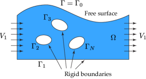
Figure 1: The fluid region is bounded above by a free surface, $\Gamma(t)$, below by a solid boundary, $\Gamma_{1}$, and internally by obstacles $\Gamma_{2}$,…,$\Gamma_{N}$. The domain is spatially periodic with all components having the same period, normalized to be $2\pi$. We allow for a background flow in which the velocity potential increases by $2\pi V_{1}$ when $x$ increases by $2\pi$ along a path passing above each of the obstacles.

2.1 Graph-based and angle-arclength parameterizations of the free surface

At a point $(\xi(\alpha,t),\eta(\alpha,t))$ we have unit tangent and normal vectors. Suppressing the dependence on $(\alpha,t)$ in the notation, they are

$$\mathbf{\hat{t}}=\frac{(\xi_{\alpha},\eta_{\alpha})}{|(\xi_{\alpha},\eta_{\alpha})|},\qquad\mathbf{\hat{n}}=\frac{(-\eta_{\alpha},\xi_{\alpha})}{|(\xi_{\alpha},\eta_{\alpha})|}.$$ (2.6)

We describe the motion of the free surface using the generic evolution equation

$$(\xi,\eta)_{t}=U\mathbf{\hat{n}}+V\mathbf{\hat{t}}.$$ (2.7)

Here $U$ is the normal velocity and $V$ is the tangential velocity of the parameterization. One part of the Hou, Lowengrub and Shelley (HLS) HLS1 ; HLS2 framework is the idea that $V$ need not be chosen according to physical principles, but instead may be chosen to enforce a favorable parameterization on the free surface. The normal velocity, however, must match that of the fluid.

In Sections 3 and 4 below, we present two methods of computing the normal velocity $U=\partial\phi/\partial n$ of the fluid on the free surface, where $\phi(x,y,t)$ is the velocity potential. A simple approach for cases when the free surface is not expected to overturn or develop steep slopes is to set $\xi(\alpha)=\alpha$ and evolve $\eta(x,t)$ in time. Setting $\xi_{t}=0$ in (2.7) and using (2.6) gives $V=\eta_{\alpha}U$ and

$$\eta_{t}=\sqrt{1+\eta_{\alpha}^{2}}\,U,\qquad U=\frac{\partial\phi}{\partial n}.$$ (2.8)

This is the standard graph-based formulation craig:sulem:93 ; zakharov68 of the water wave equations, where the Dirichlet-Neumann operator mapping the velocity potential on the free surface to the normal velocity now involves solving the Laplace equation on a multiply-connected domain. Mesh refinement can be introduced by choosing a different function $\xi(\alpha)$ such that $\xi_{\alpha}(\alpha)$ is smaller in regions requiring additional resolution. This is done in water2 for the case without obstacles to resolve small-scale features at the crests of large-amplitude standing water waves.

Hou, Lowengrub and Shelley HLS1 ; HLS2 proposed a flexible alternative to the graph-based representation that allows for overturning waves and simplifies the treatment of surface tension. Rather than evolving the Cartesian coordinates $\xi(\alpha,t)$ and $\eta(\alpha,t)$ directly, the tangent angle $\theta(\alpha,t)$ of the free surface relative to the horizontal is evolved in time. In the complex representation (2.5), we have

$$\zeta_{\alpha}=s_{\alpha}e^{i\theta},\qquad\zeta_{t}=(V+iU)e^{i\theta},$$ (2.9)

where $s_{\alpha}(\alpha,t)$ is the arclength element, defined by $s_{\alpha}=|\zeta_{\alpha}|=\sqrt{\xi_{\alpha}^{2}+\eta_{\alpha}^{2}}.$ Equating $\zeta_{\alpha t}=\zeta_{t\alpha}$ in (2.9), one finds that

$$\theta_{t}=\frac{U_{\alpha}+V\theta_{\alpha}}{s_{\alpha}},\qquad s_{\alpha t}=V_{\alpha}-\theta_{\alpha}U.$$ (2.10)

One can require a uniform parameterization in which $s_{\alpha}(\alpha,t)=L(t)/2\pi$ is independent of $\alpha$, where $L(t)$ is the length of a period of the interface. This gives

$$V_{\alpha}=\theta_{\alpha}U-\frac{1}{2\pi}\int_{0}^{2\pi}\theta_{\alpha}U\ d\alpha.$$ (2.11)

By taking the tangential velocity, $V,$ to be a solution of (2.11), we ensure that the normalized arclength parameterization is maintained at all times. When solving (2.11) for $V,$ a constant of integration must be chosen. Three suitable choices are (a) the mean of $V$ can be taken to be zero; (b) $V(0,t)=0;$ or (c) $\xi(0,t)=0$. We usually prefer (c) as it conveniently anchors the coordinate system for describing the surface.

2.2 Staying on the constraint manifold

In solving the evolution of the surface profile in the HLS framework, we must ensure that a periodic profile arises at each stage of the iteration. As we have described the HLS method so far, the curve $\zeta(\alpha)$ is represented by $\theta(\alpha)$ and $s_{\alpha}=L/2\pi$ together with two integration constants, which we take to be $\xi(0)=0$ and $\langle\eta\rangle=\frac{1}{2\pi}\int_{0}^{2\pi}\eta(\alpha)\xi_{\alpha}(\alpha)\,d\alpha=0$. The latter quantity is the average height of the free surface, which, by incompressibility, remains constant in time and can be set to 0 by a suitable vertical adjustment of the initial conditions and solid boundaries if necessary. The problem is that not every function $\theta$ and number $s_{\alpha}$ are the tangent angle and arclength element of a periodic curve (in the sense of (2.1)). We refer to those that are as being on the constraint manifold.

A drawback of the HLS formulation is that numerical error can cause the solution to deviate from this constraint manifold, e.g., in internal Runge-Kutta stages or when evolving the interface over many time steps. Internal Runge-Kutta stages typically contain $O(h^{2})$ errors that cancel out over the full step if the solution is smooth enough; thus, it is critical that the curve reconstruction not introduce $O(h^{2})$ grid oscillations.

Our idea is to evolve only $P\theta$ in time and select $P_{0}\theta$ and $s_{\alpha}$ as part of the reconstruction of $\zeta(\alpha)$ to enforce $\zeta(2\pi)=\zeta(0)+2\pi$. Here $P_{0}$ is the orthogonal projection in $L^{2}(0,2\pi;d\alpha)$ onto the constant functions while $P$ projects onto functions with zero mean,

$$P=I-P_{0},\qquad P_{0}f=\frac{1}{2\pi}\int_{0}^{2\pi}f(\alpha)\,d\alpha.$$ (2.12)

Note that $P_{0}\eta$ is the mean of $\eta$ with respect to $\alpha$ on $[0,2\pi]$, which differs from the mean in physical space, $\langle\eta\rangle=P_{0}[\eta\xi_{\alpha}]$. Given $P\theta$, we define

$$\begin{aligned} C&=P_{0}\big{[}\cos P\theta],\\ S&=P_{0}\big{[}\sin P\theta],\end{aligned}\qquad\begin{aligned} P_{0}\theta&=\operatorname{arg}(C-iS),\\ \theta&=P\theta+P_{0}\theta\end{aligned}\qquad s_{\alpha}=(C^{2}+S^{2})^{-1/2}.$$ (2.13)

We then define $\zeta_{\alpha}=s_{\alpha}e^{i\theta}$ and note that

$$\zeta(2\pi)-\zeta(0)=(s_{\alpha}e^{iP_{0}\theta})\int_{0}^{2\pi}e^{i(P\theta)(\alpha)}d\alpha=\frac{C-iS}{C^{2}+S^{2}}\big{[}2\pi(C+iS)\big{]}=2\pi.$$ (2.14)

Thus, any antiderivative $\zeta(\alpha)$ of $\zeta_{\alpha}=\xi_{\alpha}+i\eta_{\alpha}$ will lie on the constraint manifold. We also note for future reference that

$$P\big{[}\cos\theta\big{]}=\cos\theta-s_{\alpha}^{-1},\qquad P\big{[}\sin\theta\big{]}=\sin\theta.$$ (2.15)

Next, we compute the zero-mean antiderivatives

$$\xi^{\text{aux}}=\int[\xi_{\alpha}-1]\,d\alpha,\qquad\eta^{\text{aux}}=\int\eta_{\alpha}\,d\alpha$$

via the FFT. Both integrands have zero mean due to (2.14), so $\xi^{\text{aux}}$ and $\eta^{\text{aux}}$ are $2\pi$-periodic. The conditions $\xi(0)=0$ and $\langle\eta\rangle=0$ are achieved by adding integration constants

$$\xi(\alpha)=\alpha+\xi^{\text{aux}}(\alpha)-\xi^{\text{aux}}(0),\qquad\eta(\alpha)=\eta^{\text{aux}}(\alpha)-P_{0}[\eta^{\text{aux}}\xi_{\alpha}].$$ (2.16)

The $\alpha$ term in $\xi(\alpha)$ accounts for the 1 in the integrand in the formula for $\xi^{\text{aux}}$. This completes the reconstruction of $\zeta(\alpha)=\xi(\alpha)+i\eta(\alpha)$ from $P\theta$.

We compute the normal velocity, $U$, of the fluid on the reconstructed curve $\zeta(\alpha)$ as described in Sections 3 or 4 below. The evolution of $P\theta$ is obtained by applying $P$ to the first equation of (2.10),

$$(P\theta)_{t}=P\left(\frac{U_{\alpha}+V\theta_{\alpha}}{s_{\alpha}}\right).$$ (2.17)

In Appendix A, we show that $\theta$ and $s_{\alpha}$ from (2.13) satisfy (2.10) even though $P_{0}\theta$ and $s_{\alpha}$ are computed algebraically rather than by solving ODEs. We also show that (2.10) implies that the curve kinematics are correct, i.e., $(\xi_{t},\eta_{t})=U\mathbf{n}+V\mathbf{t}$. As far as the authors know, this approach of evolving $P\theta$ via (2.17) and computing $P_{0}\theta$ and $s_{\alpha}$ algebraically (rather than evolving them) is an original formulation (although a different algebraic formula for just $s_{\alpha}$ has been used previously akers2013traveling ).

We reiterate that the advantage of computing $P_{0}\theta$ and $s_{\alpha}$ from $P\theta$ is that the reconstructed curve is always on the constraint manifold. This avoids loss of accuracy in internal Runge-Kutta stages or after many steps due to grid oscillations that arise when computing periodic antiderivatives from functions with non-zero mean.

3 Cauchy Integrals and the Velocity Potential Formulation

As explained above, we let the fluid region, $\Omega,$ be $2\pi$-periodic in $x$ with free surface $\Gamma=\Gamma_{0}$, bottom boundary $\Gamma_{1}$, and cylinder boundaries $\Gamma_{2}$, …$\Gamma_{N}$. The cylinder boundaries need not be circular, but are assumed to be smooth. We view $\Omega$ as a subset of the complex plane. Let us decompose the complex velocity potential $\Phi(z)=\phi(z)+i\psi(z)$ as

$$\Phi(z)=\tilde{\Phi}(z)+\Phi_{\text{mv}}(z),$$ (3.1)

where $\tilde{\Phi}(z)=\Phi_{0}(z)+\cdots+\Phi_{N}(z)$ and

$$\Phi_{\text{mv}}(z)=V_{1}z+\sum_{j=2}^{N}a_{j}\Phi_{\text{cyl}}(z-z_{j}),\qquad\Phi_{\text{cyl}}(z)=-i\log\big{(}1-e^{iz}\big{)}.$$ (3.2)

Here $z_{j}$ is a point inside the $j$th cylinder; $V_{1}$ and the $a_{j}$ are real parameters corresponding to the background flow strength and circulation around each cylinder, divided by $2\pi$, which allow $\phi(z)$ (but not $\psi(z)$) to be multi-valued on $\Omega$; and $\tilde{\Phi}(z)$ is represented by Cauchy integrals:

$$\Phi_{0}(z) =\frac{1}{2\pi i}\int_{0}^{2\pi}\frac{1}{2}\cot\frac{\zeta_{0}(\alpha)-z}{2}\omega_{0}(\alpha)\,\zeta_{0}^{\prime}(\alpha)\,d\alpha, \text{(free surface)},$$ (3.3)

$$\Phi_{j}(z) =\frac{1}{2\pi i}\int_{0}^{2\pi}\frac{1}{2}\cot\frac{\zeta_{j}(\alpha)-z}{2}i\omega_{j}(\alpha)\,\zeta_{j}^{\prime}(\alpha)\,d\alpha, \left(\begin{gathered}\text{solid boundaries}\\ 1\leq j\leq N\end{gathered}\right).$$ (3.6)

Here $\omega_{j}(\alpha)$ is a real-valued function for $0\leq j\leq N$, and we use primes interchangeably with $\alpha$ subscripts to denote derivatives of $\zeta_{j}(\alpha)$, $\omega_{j}(\alpha)$, etc. We refer to these as Cauchy integrals as they correspond to a principal value sum of the Cauchy kernel over periodic images via a Mittag-Leffler formula ablowitzFokas , namely

$$PV\sum_{k}\frac{1}{\zeta+2\pi k-z}=\frac{1}{2}\cot\frac{\zeta-z}{2}.$$ (3.7)

We have temporarily dropped $t$ from $\zeta_{0}(\alpha,t)$ since time may be considered frozen when computing the velocity potential. The subscript $0$ is optional only for $\zeta_{0}$, $\xi_{0}$, $\eta_{0}$, $\Gamma_{0}$ and for quantities such as $s_{\alpha}$ and $\theta$ defined in terms of $\eta_{\alpha}$ and $\xi_{\alpha}$. In particular, $\Phi,\phi,\psi$ are not the same as $\Phi_{0},\phi_{0},\psi_{0}$ in our notation. The real and imaginary parts of $\tilde{\Phi}$, $\Phi_{\text{mv}}$, $\Phi_{j}$ and $\Phi_{\text{cyl}}$ will be denoted by $\tilde{\phi}$, $\tilde{\psi}$, $\phi_{\text{mv}}$, etc.

3.1 Properties of $\Phi_{\text{cyl}}(z)$ and time independence of $V_{1}$, $a_{2}$, …, $a_{N}$

We regard $\Phi_{\text{cyl}}(z)$ as a multi-valued analytic function defined on a Riemann surface with branch points $z\in 2\pi\mathbb{Z}$. On the $n$th sheet of the Riemann surface, $\Phi_{\text{cyl}}(z)$ is given by

$$\Phi_{\text{upper},n}(z)=-i\operatorname{Log}\big{(}1-e^{iz}\big{)}+2\pi n,\qquad(n\in\mathbb{Z}),$$ (3.8)

where $\operatorname{Log}(z)$ is the principal value of the logarithm. The functions (3.8) are analytic in the upper half-plane and have vertical branch cuts extending from the branch points down to $-i\infty$. Their imaginary parts are all the same, given by $-\ln|1-e^{iz}|$, which is continuous across the branch cuts (except at the branch points) and harmonic on $\mathbb{C}\setminus 2\pi\mathbb{Z}$. The real part of $\Phi_{\text{upper},n}(z)$ jumps from $2\pi(n+1/2)$ to $2\pi(n-1/2)$ when crossing a branch cut from left to right. We obtain $\Phi_{\text{cyl}}(z)$ by gluing $\Phi_{\text{upper},n}(z)$ on the left of each branch cut to $\Phi_{\text{upper},n+1}(z)$ on the right. Equivalently, we can define horizontal branch cuts $I_{k}=\big{(}2\pi k,2\pi(k+1)\big{)}\subset\mathbb{R}$ for $k\in\mathbb{Z}$ and glue $\Phi_{\text{upper},n}(z)$ to

$$\Phi_{\text{lower},m}(z)=-i\operatorname{Log}\big{(}1-e^{-iz}\big{)}+z+(2m-1)\pi,\qquad(m\in\mathbb{Z})$$ (3.9)

along $I_{n-m}$. $\Phi_{\text{lower},m}(z)$ is analytic in the lower half-plane and has vertical branch cuts extending from the points $z\in 2\pi\mathbb{Z}$ up to $+i\infty$. Both $\Phi_{\text{upper},n}(z)$ and $\Phi_{\text{lower},m}(z)$ are defined and agree with each other on the strip $z=x+iy$ with $y\in\mathbb{R}$ and $x\in I_{n-m}$, so they are analytic continuations of each other to the opposite half-plane through $I_{n-m}$. To show this, one may check that

$$\Phi_{\text{upper},0}(x)=\left(\frac{x-\pi}{2}-i\ln\sqrt{2-2\cos x}\right)=\Phi_{\text{lower},0}(x),\quad(0<x<2\pi).$$

By the identity theorem, $\Phi_{\text{upper},0}(z)=\Phi_{\text{lower},0}(z)$ on the strip $z=x+iy$ with $x\in I_{0}$ and $y\in\mathbb{R}$. The result follows using the property that $\Phi_{\text{upper},n}(z)$ is $2\pi$-periodic while $\Phi_{\text{lower},m}(z+2\pi k)=\Phi_{\text{lower},m}(z)+2\pi k$ for $k\in\mathbb{Z}$.

Following a path from some point $z_{*}$ to $z_{*}+2\pi$ that passes above all the cylinders will cause $\Phi_{\text{mv}}(z)$ to increase by $2\pi V_{1}$. The free surface is such a path. If the path passes below all the cylinders, $\Phi_{\text{mv}}(z)$ will increase by $2\pi(V_{1}+a_{2}+\cdots+a_{N})$. More complicated paths from $z_{*}$ to $z_{*}+2\pi n_{1}$ that loop $n_{j}\in\mathbb{Z}$ times around the $j$th cylinder in the counter-clockwise ($n_{j}>0$) or clockwise ($n_{j}<0$) direction relative to a path passing above all the cylinders will cause $\Phi_{\text{mv}}(z)$ to change by $2\pi(n_{1}V_{1}+n_{2}a_{2}+\cdots+n_{N}a_{N})$.

The derivative of $\Phi_{\text{cyl}}(z)$ is single-valued and has poles at the points $z\in 2\pi\mathbb{Z}$. Explicitly,

$$\Phi^{\prime}_{\text{cyl}}(z)=\frac{1}{2}-\frac{i}{2}\cot\frac{z}{2}.$$ (3.10)

A more evident antiderivative of this function is

$$\frac{z}{2}-i\log\sin\frac{z}{2},$$ (3.11)

which has the same set of possible values as $\big{[}\Phi_{\text{cyl}}(z)+\frac{\pi}{2}+i\ln 2\big{]}$ for a given $z$. However, using the principal value of the logarithm in (3.11) leads to awkward branch cuts that are difficult to explain how to glue together to obtain a multi-valued function $\Phi_{\text{cyl}}(z)$ on a Riemann surface.

It follows from the Euler equations for $\mathbf{u}=\nabla\phi$,

$$\rho\nabla\left(\phi_{t}+\frac{1}{2}\|\nabla\phi\|^{2}+\frac{p}{\rho}+gy\right)=\rho[\mathbf{u}_{t}+\mathbf{u}\cdot\nabla\mathbf{u}]+\nabla p+\rho g\mathbf{\hat{y}}=0,$$ (3.12)

that $V_{1}$ and the $a_{j}$ are independent of time. This is because the change in $\phi_{t}$ around a path encircling a cylinder or connecting $(0,y_{*})$ to $(2\pi,y_{*})$ is the negative of the change in $\frac{1}{2}\|\nabla\phi\|^{2}+\frac{p}{\rho}+gy$, which is single-valued and periodic. For the cylinders, this also follows from the Kelvin circulation theorem.

3.2 Integral equations for the densities $\omega_{j}$

Evaluation of the Cauchy integrals in (3.3) on the boundaries via the Plemelj formulas singularIntegralEquations gives the results in Table 1. When $j=k\in\{0,\dots,N\}$ and $\beta\rightarrow\alpha$, $K_{jj}(\alpha,\beta)\rightarrow\operatorname{Im}\{\zeta_{j}^{\prime\prime}(\alpha)/[2\zeta_{j}^{\prime}(\alpha)]\}$, so the apparently singular integrands are actually regular due to the imaginary part. They are automatically regular when $j\neq k$ since $\zeta_{j}(\beta)$ and $\zeta_{k}(\alpha)$ are never equal. So far $G_{kj}$ only arises with $j\neq k$; the regularizing term $(1/2)\cot[(\beta-\alpha)/2]$ will become relevant in (3.27) below.

$\displaystyle\phi_{0}(\zeta_{0}(\alpha)^{-})$ $\displaystyle=-\frac{1}{2}\omega_{0}(\alpha)+\frac{1}{2\pi}\int_{0}^{2\pi}K_{00}(\alpha,\beta)\omega_{0}(\beta)\,d\beta,$ $\displaystyle\phi_{j}(\zeta_{0}(\alpha))$ $\displaystyle=\frac{1}{2\pi}\int_{0}^{2\pi}G_{0j}(\alpha,\beta)\omega_{j}(\beta)\,d\beta,\qquad(1\leq j\leq N)$ $\displaystyle\psi_{0}(\zeta_{k}(\alpha))$ $\displaystyle=\frac{1}{2\pi}\int_{0}^{2\pi}-G_{k0}(\alpha,\beta)\omega_{0}(\beta)\,d\beta,\qquad(1\leq k\leq N)$ $\displaystyle\psi_{j}(\zeta_{j}(\alpha)^{+})$ $\displaystyle=\frac{1}{2}\omega_{j}(\alpha)+\frac{1}{2\pi}\int_{0}^{2\pi}K_{jj}(\alpha,\beta)\omega_{j}(\beta)\,d\beta,\qquad(1\leq j\leq N)$ $\displaystyle\psi_{j}(\zeta_{k}(\alpha))$ $\displaystyle=\frac{1}{2\pi}\int_{0}^{2\pi}K_{kj}(\alpha,\beta)\omega_{j}(\beta)\,d\beta,\qquad(1\leq j,k\leq N,\;\;j\neq k)$ $\displaystyle K_{kj}(\alpha,\beta)$ $\displaystyle=\operatorname{Im}\left\{\frac{\zeta_{j}^{\prime}(\beta)}{2}\cot\left(\frac{\zeta_{j}(\beta)-\zeta_{k}(\alpha)}{2}\right)\right\},\qquad(0\leq j,k\leq N)$ $\displaystyle G_{kj}(\alpha,\beta)$ $\displaystyle=\operatorname{Re}\left\{\frac{\zeta_{j}^{\prime}(\beta)}{2}\cot\left(\frac{\zeta_{j}(\beta)-\zeta_{k}(\alpha)}{2}\right)-\delta_{kj}\frac{1}{2}\cot\frac{\beta-\alpha}{2}\right\}.$

Table 1: Evaluation of the Cauchy integrals on the boundaries. The Plemelj formulas singularIntegralEquations are used to take one-sided limits from within $\Omega$, where the positive side of a parameterized curve lies to the left. In the last formula, $\delta_{kj}=1$ if $k=j$ and 0 otherwise. This term will be relevant in (3.27) below.

Next we consider the operator $\mathbb{B}$ mapping the dipole densities $\omega_{j}$ to the values of $\tilde{\phi}$ on $\Gamma_{0}^{-}$ and $\tilde{\psi}$ on $\Gamma_{k}^{+}$ for $1\leq k\leq N$. Recall from (3.1) that a tilde denotes the contribution of the Cauchy integrals to the velocity potential. We regard the functions $\omega_{j}$, $\tilde{\phi}|_{\Gamma_{0}^{-}}$ and $\tilde{\psi}|_{\Gamma_{k}^{+}}$ as elements of the (real) Hilbert space $L^{2}(0,2\pi)$. They are functions of $\alpha$, and we do not assume the curves $\zeta_{j}(\alpha)$ are parameterized by arclength. The operator $\mathbb{B}$ has a block structure arising from the formulas in Table 1. For example, when $N=2$, $\mathbb{B}$ has the form

$$\mathbb{B}\omega:=\begin{pmatrix}\tilde{\phi}|_{\Gamma_{0}^{-}}\\ \tilde{\psi}|_{\Gamma_{1}^{+}}\\ \tilde{\psi}|_{\Gamma_{2}^{+}}\end{pmatrix}=\left[\begin{pmatrix}-\frac{1}{2}\mathbb{I}\\ &\frac{1}{2}\mathbb{I}\\ &&\frac{1}{2}\mathbb{I}\end{pmatrix}+\begin{pmatrix}\mathbb{K}_{00}&\mathbb{G}_{01}&\mathbb{G}_{02}\\ -\mathbb{G}_{10}&\mathbb{K}_{11}&\mathbb{K}_{12}\\ -\mathbb{G}_{20}&\mathbb{K}_{21}&\mathbb{K}_{22}\end{pmatrix}\right]\begin{pmatrix}\omega_{0}\\ \omega_{1}\\ \omega_{2}\end{pmatrix},$$ (3.13)

where

$$\mathbb{K}_{kj}\omega_{j}=\frac{1}{2\pi}\int_{0}^{2\pi}K_{kj}(\cdot,\beta)\omega_{j}(\beta)\,d\beta,\qquad\mathbb{G}_{kj}\omega_{j}=\frac{1}{2\pi}\int_{0}^{2\pi}G_{kj}(\cdot,\beta)\omega_{j}(\beta)\,d\beta.$$ (3.14)

Here $k$ and $j$ are fixed; there is no implied summation over repeated indices. Up to rescaling of the rows by factors of $-2$ or $2$, the operator $\mathbb{B}$ is a compact perturbation of the identity, so has a finite-dimensional kernel. The structure of $\mathbb{B}$ for $N>2$ is easily extended as in (3.13), with the entries on the diagonal continuing to be of the form $\frac{1}{2}\mathbb{I}$ for each new obstacle. The dimension of the kernel turns out to be $N-1$, spanned by the functions $\omega=\mathbf{1}_{m}$ given by

$$(\mathbf{1}_{m})_{j}(\alpha)=\left\{\begin{array}[]{cc}1,&\quad j=m\\ 0,&\quad j\neq m\end{array}\right\},\qquad(0\leq j\leq N,\quad 2\leq m\leq N).$$ (3.15)

Indeed, if $\omega=\mathbf{1}_{m}$ with $m\geq 2$, then each $\Phi_{j}(z)$ is zero everywhere if $j\neq m$ and is zero outside the $m$th cylinder if $j=m$, including along $\zeta_{m}(\alpha)^{+}$. Summing over $j$ and restricting the real part to $\Gamma_{0}^{-}$ or the imaginary part to $\Gamma_{k}^{+}$, $1\leq k\leq N$, gives zero for each component of $\mathbb{B}\omega$ in (3.13). In Section 6 we will prove that all the vectors in $\ker\mathbb{B}$ are linear combinations of these, and that the range of $\mathbb{B}$ is complemented by the same functions $\mathbf{1}_{m}$, $2\leq m\leq N$. The operator

$$\mathbb{A}\omega=\mathbb{B}\omega-\sum_{m=2}^{N}\mathbf{1}_{m}\langle\mathbf{1}_{m},\omega\rangle,\quad\langle\mu,\omega\rangle=\sum_{j=0}^{N}\frac{1}{2\pi}\int_{0}^{2\pi}\mu_{j}(\alpha)\omega_{j}(\alpha)\,d\alpha.$$ (3.16)

is then an invertible rank $N-1$ correction of $\mathbb{B}$. We remark that (3.16) is tailored to the case where $V_{1}$, $a_{2}$, …, $a_{N}$ in the representation (3.1) for $\Phi$ are given and the constant values $\psi|_{k}$ are unknown. The case when $\psi$ is completely specified on $\Gamma_{k}$ for $1\leq k\leq N$ is discussed in Appendix B.

In the water wave problem, we need to evaluate the normal derivative of $\phi$ on the free surface to obtain the normal velocity $U$. In the present algorithm, we evolve $\tilde{\varphi}=\tilde{\phi}|_{\Gamma}$ in time, so its value is known when computing $U$. On the bottom boundary and cylinders, the stream function $\psi$ should be constant (to prevent the fluid from penetrating the walls). Let $\psi|_{k}$ denote the constant value of $\psi$ on the $k$th boundary. We are free to set $\psi|_{1}=0$ on the bottom boundary but do not know the other $\psi|_{k}$ in advance. We claim that $\psi|_{k}=\langle\mathbf{1}_{k},\omega\rangle$ for $2\leq k\leq N$. From (3.1),

$$\psi(z)=\tilde{\psi}(z)+\psi_{\text{mv}}(z)=\psi|_{k}=\text{const},\qquad\quad(z\in\Gamma_{k}^{+}\,,\;1\leq k\leq N).$$ (3.17)

This is achieved by solving

$$\mathbb{A}\omega=b,\qquad b_{0}(\alpha)=\tilde{\varphi}(\alpha),\quad b_{k}(\alpha)=-\psi_{\text{mv}}(\zeta_{k}(\alpha)),\quad(1\leq k\leq N),$$ (3.18)

which gives $\tilde{\psi}|_{\Gamma_{k}^{+}}=(\mathbb{B}\omega)_{k}=b_{k}+\sum_{m\geq 2}\delta_{km}\langle\mathbf{1}_{m},\omega\rangle=-\psi_{\text{mv}}|_{\Gamma_{k}}+\langle\mathbf{1}_{k},\omega\rangle$ for $2\leq k\leq N$. Thus, $\psi(z)=\psi|_{k}=\langle\mathbf{1}_{k},\omega\rangle$ is constant for $z\in\Gamma_{k}^{+}$, as required. (For $k=1$, each $\delta_{km}$ is zero and $\psi|_{k}=0$.)

3.3 Numerical discretization

We adopt a collocation-based numerical method and replace the integrals in Table 1 with trapezoidal rule sums. Let $M_{0}$, …, $M_{N}$ denote the number of grid points chosen to discretize the free surface and solid boundaries, respectively. Let $\alpha_{kl}=2\pi l/M_{k}$ for $0\leq l<M_{k}$, and define $K_{kj,ml}=K_{kj}(\alpha_{km},\alpha_{jl})/M_{j}$ and $G_{kj,ml}=G_{kj}(\alpha_{km},\alpha_{jl})/M_{j}$ so that

$$\mathbb{K}_{kj}\omega_{j}(\alpha_{km})\approx\sum_{l=0}^{M_{j}-1}K_{kj,ml}\omega_{j}(\alpha_{jl}),\qquad\mathbb{G}_{kj}\omega_{j}(\alpha_{km})\approx\sum_{l=0}^{M_{j}-1}G_{kj,ml}\omega_{j}(\alpha_{jl}).$$

When $N=2$, the system (3.18) becomes

$$\left(\begin{array}[]{c|c|c}-\frac{1}{2}I_{0}+K_{00}&G_{01}&G_{02}\\[2.0pt] \hline\cr\raisebox{-2.0pt}{$-G_{10}$}&\raisebox{-2.0pt}{$\frac{1}{2}I_{1}+K_{11}$}&\raisebox{-2.0pt}{$K_{12}$}\\[4.0pt] \hline\cr\raisebox{-2.0pt}{$-G_{20}$}&\raisebox{-2.0pt}{$K_{21}$}&\raisebox{-2.0pt}{$\frac{1}{2}I_{2}+K_{22}-E_{2}$}\end{array}\right)\begin{pmatrix}\omega_{0}\\ \omega_{1}\\ \omega_{2}\end{pmatrix}=\begin{pmatrix}\tilde{\varphi}\\ -\psi_{\text{mv}}|_{\Gamma_{1}}\\ -\psi_{\text{mv}}|_{\Gamma_{2}}\end{pmatrix},$$ (3.19)

where $E_{m}=M_{m}^{-1}ee^{T}$ with $e=(1;1;\dots;1)\in\mathbb{R}^{M_{m}}$ represents $\mathbf{1}_{m}\langle\mathbf{1}_{m},\cdot\rangle$ and the right-hand side is evaluated at the grid points. For example, in (3.19) with $N=2$, $-\psi_{\text{mv}}|_{\Gamma_{1}}$ has components $-V_{1}\eta_{1}(\alpha_{1m})-a_{2}\psi_{\text{cyl}}(\zeta_{1}(\alpha_{1m})-z_{2})$ for $0\leq m<M_{1}$. The generalization to $N>2$ solid boundaries is straightforward, with additional diagonal blocks of the form $\frac{1}{2}I+K_{jj}-E_{j}$.

3.4 Computation of the normal velocity

Once the $\omega_{j}$ are known from solving (3.19), we can compute $U=\partial\phi/\partial n$ on the free surface, which is what is needed to evolve both $\tilde{\varphi}$ and $\zeta(\alpha,t)$ using the HLS machinery. From (3.10), we see that the multi-valued part of the potential, $\phi_{\text{mv}}(z)=\operatorname{Re}\{\Phi_{\text{mv}}(z)\}$, contributes

$$s_{\alpha}\frac{\partial\phi_{\text{mv}}}{\partial n}=\operatorname{Re}\{(\phi_{\text{mv},x}-i\phi_{\text{mv},y})(n_{1}+in_{2})s_{\alpha}\}=\operatorname{Re}\{\Phi_{\text{mv}}^{\prime}(\zeta(\alpha))i\zeta^{\prime}(\alpha)\}$$ (3.20)

$$\quad\;\;=-\bigg{(}V_{1}+\frac{1}{2}\sum_{j=2}^{N}a_{j}\bigg{)}\eta^{\prime}(\alpha)+\sum_{j=2}^{N}a_{j}\operatorname{Re}\left\{\frac{1}{2}\cot\left(\frac{\zeta(\alpha)-z_{j}}{2}\right)\zeta^{\prime}(\alpha)\right\},$$

where $s_{\alpha}=|\zeta^{\prime}(\alpha)|$ and $\eta(\alpha)=\operatorname{Im}\zeta(\alpha)$. This normal derivative (indeed the entire gradient) of $\phi_{\text{mv}}$ is single-valued. We can differentiate (3.3) under the integral sign and integrate by parts to obtain

$$\Phi_{j}^{\prime}(z)=\frac{1}{2\pi}\int_{0}^{2\pi}\frac{1}{2}\cot\frac{\zeta_{j}(\beta)-z}{2}\omega_{j}^{\prime}(\beta)\,d\beta,\qquad(1\leq j\leq N).$$ (3.21)

We can then evaluate

$$s_{\alpha}\frac{\partial\phi_{j}}{\partial n} =\operatorname{Re}\{(\phi_{j,x}-i\phi_{j,y})(n_{1}+in_{2})s_{\alpha}\}=\operatorname{Re}\{\Phi_{j}^{\prime}(\zeta(\alpha))i\zeta^{\prime}(\alpha)\}$$ (3.22)

$$=\frac{1}{2\pi}\int_{0}^{2\pi}K_{j0}(\beta,\alpha)\omega_{j}^{\prime}(\beta)\,d\beta,\qquad(1\leq j\leq N).$$

Note that the integration variable $\beta$ now appears in the first slot of $K_{j0}$. For $j=0$, after integrating (3.3) by parts, we obtain

$$\Phi_{0}^{\prime}(z)=\frac{1}{2\pi i}\int_{0}^{2\pi}\frac{1}{2}\cot\frac{\zeta(\beta)-z}{2}\omega_{0}^{\prime}(\beta)\,d\beta.$$ (3.23)

Taking the limit as $z\rightarrow\zeta(\alpha)^{-}$ (or as $z\rightarrow\zeta(\alpha)^{+}$) gives

$$\Phi_{0}^{\prime}(\zeta(\alpha)^{\pm}) =\lim_{z\rightarrow\zeta(\alpha)^{\pm}}\frac{1}{2\pi i}\int_{0}^{2\pi}\frac{\zeta^{\prime}(\beta)}{2}\cot\frac{\zeta(\beta)-z}{2}\left(\frac{\omega_{0}^{\prime}(\beta)}{\zeta^{\prime}(\beta)}\right)\,d\beta$$ (3.24)

$$=\pm\frac{\omega_{0}^{\prime}(\alpha)}{2\zeta^{\prime}(\alpha)}+\frac{1}{2\pi i}PV\!\!\int_{0}^{2\pi}\frac{1}{2}\cot\frac{\zeta(\beta)-\zeta(\alpha)}{2}\,\omega_{0}^{\prime}(\beta)\,d\beta$$

where PV indicates a principal value integral and we used the Plemelj formula to take the limit. Finally, we regularize the integral using the Hilbert transform,

$$\mathbb{H}f(\alpha)=\frac{1}{\pi}PV\int_{0}^{2\pi}\frac{1}{2}\cot\frac{\alpha-\beta}{2}f(\beta)\,d\beta$$ (3.25)

to obtain

$$\zeta^{\prime}(\alpha)\Phi_{0}^{\prime}(\zeta(\alpha)^{\pm})=\pm\frac{1}{2}\omega_{0}^{\prime}(\alpha)+\frac{i}{2}\mathbb{H}\omega_{0}^{\prime}(\alpha)$$ (3.26)

$$\qquad\qquad+\frac{1}{2\pi i}\int_{0}^{2\pi}\left[\frac{\zeta^{\prime}(\alpha)}{2}\cot\frac{\zeta(\beta)-\zeta(\alpha)}{2}-\frac{1}{2}\cot\frac{\beta-\alpha}{2}\right]\omega_{0}^{\prime}(\beta)\,d\beta.$$

The term in brackets approaches $-\zeta^{\prime\prime}(\alpha)/[2\zeta^{\prime}(\alpha)]$ as $\beta\rightarrow\alpha$, so the integrand is not singular. The symbol of $\mathbb{H}$ is $\hat{H}_{k}=-i\operatorname{sgn}k$, so it can be computed accurately and efficiently using the FFT. Using $s_{\alpha}\partial\phi_{0}/\partial n=\operatorname{Re}\{i\zeta^{\prime}(\alpha)\Phi_{0}^{\prime}(\zeta(\alpha)^{-})\}$, we find

$$s_{\alpha}\frac{\partial\phi_{0}}{\partial n} =-\frac{1}{2}\mathbb{H}\omega_{0}^{\prime}(\alpha)-\frac{1}{2\pi}\int_{0}^{2\pi}G_{00}(\beta,\alpha)\omega_{0}^{\prime}(\beta)\,d\beta,$$ (3.27)

which we evaluate with spectral accuracy using the trapezoidal rule. The desired normal velocity $U$ is the sum of (3.20), (3.22) for $1\leq j\leq N$, and (3.27), all divided by $s_{\alpha}$.

3.5 Time evolution of the surface velocity potential

The last step is to find the evolution equation for $\tilde{\varphi}(\alpha,t)=\tilde{\phi}(\zeta(\alpha,t),t)$, where $\tilde{\phi}$ is the component of the velocity potential represented by Cauchy integrals. The chain rule gives

$$\tilde{\varphi}_{t}=\nabla\tilde{\phi}\cdot\zeta_{t}+\tilde{\phi}_{t},\qquad\zeta_{t}=U\mathbf{\hat{n}}+V\mathbf{\hat{s}}.$$ (3.28)

We note that $\tilde{\phi}_{t}=\phi_{t}$, and the unsteady Bernoulli equation gives

$$\phi_{t}=-\frac{1}{2}|\nabla\phi|^{2}-p/\rho-g\eta_{0}+C(t),$$ (3.29)

where $p$ is the pressure, $\rho$ is the fluid density, $g$ is the acceleration of gravity, and $C(t)$ is an arbitrary function of time but not space. At the free surface, the Laplace-Young condition for the pressure is $p=p_{0}-\rho\tau\kappa$, where $\kappa=\theta_{\alpha}/s_{\alpha}$ is the curvature and $\rho\tau$ is the surface tension. The constant $p_{0}$ may be set to zero without loss of generality. We therefore have

$$\tilde{\varphi}_{t}=(\tilde{\varphi}_{\alpha}/s_{\alpha})V+(\partial\tilde{\phi}/\partial n)U-\frac{1}{2}|\nabla\phi|^{2}-g\,\eta(\alpha,t)+\tau\frac{\theta_{\alpha}}{s_{\alpha}}+C(t),$$ (3.30)

where $\zeta=\xi+i\eta$, $\zeta_{\alpha}=s_{\alpha}e^{i\theta}$, and $|\nabla\phi|^{2}=(\varphi_{\alpha}/s_{\alpha})^{2}+(\partial\phi/\partial n)^{2}$. These equations are valid for arbitrary parameterizations $\zeta_{j}(\alpha,t)$ and choices of tangential component of velocity $V$ for the curve. In particular, they are valid in the HLS framework described in Section 2. $C(t)$ can be taken to be 0 or chosen to project out the spatial mean of the right-hand side, for example.

4 Layer Potentials and the Vortex Sheet Strength Formulation

We now give an alternate formulation of the water wave problem in which the vortex sheet strength is evolved in time rather than the single-valued part of the velocity potential at the free surface. We also replace the constant stream function boundary conditions on the rigid boundaries by the equivalent condition that the normal velocity is zero there. Elimination of the stream function provides a pathway for generalization to 3D. However, in the 2D algorithm presented here, we continue to take advantage of the connection between layer potentials and Cauchy integrals; see Appendix C.

4.1 Vortex sheet strength and normal velocities on the boundaries

In this section, the evolution equation at the free surface will be written in terms of the vortex sheet strength $\gamma_{0}(\alpha)=-\omega_{0}^{\prime}(\alpha)$. We also define

$$\gamma_{0}(\alpha)=-\omega_{0}^{\prime}(\alpha),\qquad\quad\gamma_{j}(\alpha)=\omega_{j}^{\prime}(\alpha),\qquad(1\leq j\leq N).$$ (4.1)

Expressing (3.21) and (3.23) in terms of the $\gamma_{j}$, we see that the $j$th boundary contributes a term $\mathbf{u}_{j}=(u_{j},v_{j})=(\phi_{j,x},\phi_{j,y})$ to the fluid velocity given by

$$(u_{0}-iv_{0})(z) =\frac{1}{2\pi i}\int_{0}^{2\pi}\frac{1}{2}\cot\frac{z-\zeta_{0}(\beta)}{2}\gamma_{0}(\beta)\,d\beta,$$ (4.2)

$$(u_{j}-iv_{j})(z) =-\frac{1}{2\pi i}\int_{0}^{2\pi}\frac{1}{2}\cot\frac{z-\zeta_{j}(\beta)}{2}i\gamma_{j}(\beta)\,d\beta,\quad(1\leq j\leq N).$$

The calculation in (3.24) and a similar one for $\Phi_{j}^{\prime}(\zeta_{k}(\alpha)^{\pm})$ then gives

$$(u_{0}-iv_{0})(\zeta_{k}(\alpha)^{\pm}) =\mp\frac{\delta_{k0}}{2}\gamma_{0}(\alpha)\frac{\zeta^{\prime}(\alpha)^{*}}{s_{\alpha}^{2}}+W_{k0}^{*}(\alpha), \;\;(0\leq k\leq N),$$ (4.3)

$$(u_{j}-iv_{j})(\zeta_{k}(\alpha)^{\pm}) =\mp\frac{\delta_{kj}}{2}\gamma_{j}(\alpha)\frac{\big{(}i\zeta_{j}^{\prime}(\alpha)\big{)}^{*}}{s_{j,\alpha}^{2}}+W_{kj}^{*}(\alpha), \left(\begin{gathered}0\leq k\leq N\\ 1\leq j\leq N\end{gathered}\right).$$

Here $W_{kj}^{*}(\alpha)=W_{kj1}(\alpha)-iW_{kj2}(\alpha)$ are the Birkhoff-Rott integrals obtained by substituting $z=\zeta_{k}(\alpha)$ in the right-hand side of (4.2) and interpreting the integral in the principal value sense if $k=j$; see (D.1) in Appendix D. The resulting singular integrals (when $k=j$) can be regularized by the Hilbert transform, as we did in (3.26). The vector notation $\mathbf{W}_{kj}(\alpha)=\big{(}W_{kj1}(\alpha),W_{kj2}(\alpha)\big{)}$ will also be useful below.

Although there is no fluid outside the domain $\Omega$, we can still evaluate the layer potentials and their gradients there. In (4.3), the tangential component of $\mathbf{u}_{0}$ jumps by $-\gamma_{0}(\alpha)/s_{\alpha}$ on crossing the free surface $\Gamma_{0}$ while the normal component of $\mathbf{u}_{0}$ and all components of the other $\mathbf{u}_{j}$’s are continuous across $\Gamma_{0}$. By contrast, if $1\leq k\leq N$, the normal component of $\mathbf{u}_{k}$ jumps by $-\gamma_{k}(\alpha)/s_{k,\alpha}$ on crossing the solid boundary $\Gamma_{k}$, whereas the tangential component of $\mathbf{u}_{k}$ and all components of the other $\mathbf{u}_{j}$’s are continuous across $\Gamma_{k}$. Here crossing means from the right $(-)$ side to the left $(+)$ side.

In this formulation, we need to compute $U=\partial\phi/\partial n$ to evolve the free surface and set $\partial\phi/\partial n=0$ on all the other boundaries. We have already derived formulas for $\partial\phi/\partial n$ on the free surface in (3.20), (3.22) and (3.27). Nearly identical derivations in which $\Gamma_{0}$ is replaced by $\Gamma_{k}$ yield

$$s_{k,\alpha}\frac{\partial\phi_{\text{mv}}}{\partial n_{k}} =-\bigg{(}V_{1}+\frac{1}{2}\sum_{j=2}^{N}a_{j}\bigg{)}\eta_{k}^{\prime}(\alpha)+\sum_{j=2}^{N}a_{j}\operatorname{Re}\left\{\textstyle\frac{1}{2}\cot\left(\frac{\zeta_{k}(\alpha)-z_{j}}{2}\right)\zeta_{k}^{\prime}(\alpha)\right\},$$

$$s_{k,\alpha}\frac{\partial\phi_{0}}{\partial n_{k}} =\frac{\delta_{k0}}{2}\mathbb{H}\gamma_{0}(\alpha)+\frac{1}{2\pi}\int_{0}^{2\pi}G_{0k}(\beta,\alpha)\gamma_{0}(\beta)\,d\beta,$$ (4.4)

$$s_{k,\alpha}\frac{\partial\phi_{j}}{\partial n_{k}} =-\frac{\delta_{kj}}{2}\gamma_{j}(\alpha)+\frac{1}{2\pi}\int_{0}^{2\pi}K_{jk}(\beta,\alpha)\gamma_{j}(\beta)\,d\beta,\quad\left(\begin{aligned} 0\leq k\leq N\\ 1\leq j\leq N\end{aligned}\right),$$

where $0\leq k\leq N$ in the first two equations. Here $K_{kj}(\alpha,\beta)$ and $G_{kj}(\alpha,\beta)$ are as in Table 1 above. Since $\gamma_{0}$ is evolved in time, it is a known quantity in the layer potential calculations. Given $\gamma_{0}$, we compute $\gamma_{1},\dots,\gamma_{N}$ by solving the coupled system obtained by setting $\partial\phi/\partial n=0$ on the solid boundaries. When $N=3$, the system looks like

$$\left(\begin{array}[]{c|c|c}-\frac{1}{2}\mathbb{I}+\mathbb{K}_{11}^{*}&\mathbb{K}_{21}^{*}&\mathbb{K}_{31}^{*}\\[2.0pt] \hline\cr\raisebox{-2.0pt}{$\mathbb{K}_{12}^{*}$}&\raisebox{-2.0pt}{$-\frac{1}{2}\mathbb{I}+\mathbb{K}_{22}^{*}$}&\raisebox{-2.0pt}{$\mathbb{K}_{32}^{*}$}\\[4.0pt] \hline\cr\raisebox{-2.0pt}{$\mathbb{K}_{13}^{*}$}&\raisebox{-2.0pt}{$\mathbb{K}_{23}^{*}$}&\raisebox{-2.0pt}{$-\frac{1}{2}\mathbb{I}+\mathbb{K}_{33}^{*}$}\end{array}\right)\!\!\begin{pmatrix}\gamma_{1}\\ \gamma_{2}\\ \gamma_{3}\end{pmatrix}=\begin{pmatrix}-\mathbb{G}_{01}^{*}\gamma_{0}-s_{1,\alpha}\frac{\partial\phi_{\text{mv}}}{\partial n_{1}}\\[3.0pt] -\mathbb{G}_{02}^{*}\gamma_{0}-s_{2,\alpha}\frac{\partial\phi_{\text{mv}}}{\partial n_{2}}\\[3.0pt] -\mathbb{G}_{03}^{*}\gamma_{0}-s_{3,\alpha}\frac{\partial\phi_{\text{mv}}}{\partial n_{3}}\end{pmatrix}\!,$$ (4.5)

where

$$\mathbb{K}_{jk}^{*}\gamma_{j}=\frac{1}{2\pi}\int_{0}^{2\pi}K_{jk}(\beta,\cdot)\gamma_{j}(\beta)\,d\beta,\quad\mathbb{G}_{jk}^{*}\gamma_{j}=\frac{1}{2\pi}\int_{0}^{2\pi}G_{jk}(\beta,\cdot)\gamma_{j}(\beta)\,d\beta.$$ (4.6)

The system for $N>3$ has an identical structure. The matrices representing $\mathbb{K}_{jk}^{*}$ and $\mathbb{G}_{jk}^{*}$ in the collocation scheme have entries

$$(K_{jk}^{\dagger})_{ml} =(M_{k}/M_{j})K_{jk,lm}=K_{jk}(\alpha_{jl},\alpha_{km})/M_{j},$$ (4.7)

$$(G_{jk}^{\dagger})_{ml} =(M_{k}/M_{j})G_{jk,lm}=G_{jk}(\alpha_{jl},\alpha_{km})/M_{j}.$$

Here a dagger is used in place of a transpose symbol as a reminder to also re-normalize the quadrature weights. Once $\gamma_{0},\dots,\gamma_{N}$ are known, the normal velocity $U$ is given by

$$U=\frac{1}{s_{\alpha}}\bigg{[}\frac{1}{2}\mathbb{H}\gamma_{0}+\mathbb{G}_{00}^{*}\gamma_{0}+\sum_{j=1}^{N}\mathbb{K}_{j0}^{*}\gamma_{j}+s_{\alpha}\frac{\partial\phi_{\text{mv}}}{\partial n_{0}}\bigg{]}.$$ (4.8)

In Section 6, we will show that in the general case, with $N$ arbitrary, the system (4.5) is invertible. In practice, the discretized version is well-conditioned once enough grid points $M_{j}$ are used on each boundary $\Gamma_{j}$.

4.2 The evolution equation for $\gamma_{0}$

In the case without solid boundaries (i.e., the case of a fluid of infinite depth and in the absence of the obstacles), we only have $\gamma_{0}$ to consider. The appendix of ambroseMasmoudi1 details how to use the Bernoulli equation to find the equation for $\gamma_{0}$ in this case. This is a version of a calculation contained in BMO . The argument of ambroseMasmoudi1 and BMO for finding the $\gamma_{0,t}$ equation considers two fluids with positive densities; after deriving the equation, one of the densities can be set equal to zero. We present here an alternative calculation that only requires consideration of a single fluid, accounts for the solid boundaries, and leads to simpler formulas to implement numerically. Connections to the results of ambroseMasmoudi1 and BMO are worked out in Appendix D.

The main observation that we use to derive an equation for $\gamma_{0,t}$ is that $\phi_{t}$ is a solution of the Laplace equation in $\Omega$ with homogeneous Neumann conditions at the solid boundaries and a Dirichlet condition (the Bernoulli equation) at the free surface. Decomposing $\phi=\tilde{\phi}+\phi_{\text{mv}}$ as before, we have $\phi_{t}=\tilde{\phi}_{t}$ since $\phi_{\text{mv}}$ is time-independent. The Dirichlet condition at the free surface is then

$$\tilde{\phi}_{t}=-\frac{1}{2}|\nabla\phi|^{2}-\frac{p}{\rho}-g\eta_{0}.$$ (4.9)

Let

$$\mathbf{W}(\alpha)=\mathbf{W}_{00}(\alpha)+\mathbf{W}_{01}(\alpha)+\cdots+\mathbf{W}_{0N}(\alpha)+\nabla\phi_{\text{mv}}(\zeta(\alpha))$$ (4.10)

denote the contribution of the Birkhoff-Rott integrals from all the layer potentials evaluated at the free surface, plus the velocity due to the multi-valued part of the potential. By (4.3),

$$\nabla\phi(\zeta(\alpha))=\mathbf{W}+\frac{\gamma_{0}}{2s_{\alpha}}\mathbf{\hat{t}},\qquad\quad\frac{1}{2}|\nabla\phi|^{2}=\frac{1}{2}\mathbf{W}\cdot\mathbf{W}+\frac{\gamma_{0}}{2s_{\alpha}}\mathbf{W}\cdot\mathbf{\hat{t}}+\frac{\gamma_{0}^{2}}{8s_{\alpha}^{2}}.$$ (4.11)

To evaluate the left-hand side of (4.9), we differentiate (3.3) with $z$ fixed to obtain

$$\Phi_{0,t}(z) =\frac{1}{2\pi i}\int_{0}^{2\pi}\frac{\zeta^{\prime}(\beta)}{2}\cot\frac{\zeta(\beta)-z}{2}\left(\omega_{0,t}(\beta)-\frac{\zeta_{t}(\beta)}{\zeta^{\prime}(\beta)}\omega_{0}^{\prime}(\beta)\right)\,d\beta,$$ (4.12)

$$\Phi_{j,t}(z) =\frac{1}{2\pi}\int_{0}^{2\pi}\frac{\zeta_{j}^{\prime}(\beta)}{2}\cot\frac{\zeta_{j}(\beta)-z}{2}\omega_{j,t}(\beta)\,d\beta,\qquad(1\leq j\leq N),$$

where we used $\partial_{t}\big{\{}(\zeta^{\prime}/2)\cot[(\zeta-z)/2]\big{\}}=\partial_{\beta}\big{\{}(\zeta_{t}/2)\cot[(\zeta-z)/2]\big{\}}$ and integrated by parts. Here a prime indicates $\partial_{\beta}$ (i.e. $\partial_{\alpha}$) and a subscript $t$ indicates $\partial_{t}$. We continue to suppress $t$ in the arguments of functions, keeping in mind that the solid boundaries do not move. Letting $z\rightarrow\zeta(\alpha)^{-}$ and using (4.1) as well as $\zeta_{t}=(V+iU)\zeta^{\prime}/s_{\alpha}$, we obtain

$$\Phi_{0,t}(\zeta(\alpha)^{-}) =-\frac{1}{2}\omega_{0,t}(\alpha)-\frac{V+iU}{2s_{\alpha}}\gamma_{0}(\alpha)$$ (4.13)

$$\qquad\quad+\frac{1}{2\pi i}PV\!\!\int_{0}^{2\pi}\frac{\zeta^{\prime}(\beta)}{2}\cot\frac{\zeta(\beta)-\zeta(\alpha)}{2}\omega_{0,t}(\beta)\,d\beta$$

$$\qquad\quad+\frac{1}{2\pi i}PV\!\!\int_{0}^{2\pi}\frac{\zeta_{t}(\beta)}{2}\cot\frac{\zeta(\beta)-\zeta(\alpha)}{2}\gamma_{0}(\beta)\,d\beta,$$

$$\Phi_{j,t}(\zeta(\alpha)) =\frac{1}{2\pi}\int_{0}^{2\pi}\frac{\zeta_{j}^{\prime}(\beta)}{2}\cot\frac{\zeta_{j}(\beta)-\zeta(\alpha)}{2}\omega_{j,t}(\beta)\,d\beta,\qquad(1\leq j\leq N).$$

Next we take the real part, sum over $j\in\{0,\dots,N\}$ to get $\tilde{\phi}_{t}$ at the free surface, and use the Bernoulli equation (4.9). The first $PV$ integral becomes regular when the real part is taken, so we can differentiate under the integral sign and integrate by parts in the next step. Finally, we differentiate with respect to $\alpha$, which converts $-(1/2)\omega_{0,t}(\alpha)$ into $(1/2)\gamma_{0,t}(\alpha)$; integrate by parts to convert the $\omega_{j,t}$ terms in the integrals into $-\gamma_{j,t}$ terms; and use the boundary condition for the pressure (the Laplace-Young condition, $p=p_{0}-\rho\tau\kappa$) to obtain

$$\left(\frac{1}{2}\mathbb{I}+\mathbb{K}_{00}^{*}\right)\gamma_{0,t}-\sum_{j=1}^{N}\mathbb{G}_{j0}^{*}\gamma_{j,t}$$ (4.14)

$$\qquad\quad=\frac{\partial}{\partial\alpha}\left(-\frac{1}{2}\mathbf{W}\cdot\mathbf{W}+\frac{(V-\mathbf{W}\cdot\mathbf{\hat{t}})}{2s_{\alpha}}\gamma_{0}-\frac{\gamma_{0}^{2}}{8s_{\alpha}^{2}}+\tau\frac{\theta_{\alpha}}{s_{\alpha}}-g\eta_{0}-\mathbb{F}_{00}\gamma_{0}\right),$$

where

$$\mathbb{F}_{00}\gamma_{0}(\alpha)=\frac{1}{2\pi}PV\!\!\int_{0}^{2\pi}\operatorname{Im}\left\{\frac{\zeta_{t}(\beta)}{2}\cot\frac{\zeta(\beta)-\zeta(\alpha)}{2}\right\}\gamma_{0}(\beta)\,d\beta.$$ (4.15)

The additional equations needed to solve for the $\gamma_{j,t}$ can be obtained by differentiating (4.5) with respect to time; note that all the $K_{jk}$ terms correspond to rigid boundaries that do not change in time. Equivalently, the $\gamma_{j,t}$ can be interpreted as the layer potential densities needed to enforce homogeneous Neumann boundary conditions on $\phi_{t}$ on the solid boundaries,

$$s_{k,\alpha}\frac{\partial\phi_{t}}{\partial n_{k}}=\sum_{j=0}^{N}\operatorname{Re}\{\Phi_{j,t}^{\prime}(\zeta_{k}(\alpha)^{+})i\zeta_{k}^{\prime}(\alpha)\}=0,\qquad(1\leq k\leq N).$$ (4.16)

Either calculation yields the same set of additional linear equations, illustrated here in the $N=3$ case, with identical structure when $N>3$:

$$\left(\begin{array}[]{c|c|c|c}\mathbb{G}_{01}^{*}&-\frac{1}{2}\mathbb{I}+\mathbb{K}_{11}^{*}&\mathbb{K}_{21}^{*}&\mathbb{K}_{31}^{*}\\[2.0pt] \hline\cr\raisebox{-2.0pt}{$\mathbb{G}_{02}^{*}$}&\raisebox{-2.0pt}{$\mathbb{K}_{12}^{*}$}&\raisebox{-2.0pt}{$-\frac{1}{2}\mathbb{I}+\mathbb{K}_{22}^{*}$}&\raisebox{-2.0pt}{$\mathbb{K}_{32}^{*}$}\\[4.0pt] \hline\cr\raisebox{-2.0pt}{$\mathbb{G}_{03}^{*}$}&\raisebox{-2.0pt}{$\mathbb{K}_{13}^{*}$}&\raisebox{-2.0pt}{$\mathbb{K}_{23}^{*}$}&\raisebox{-2.0pt}{$-\frac{1}{2}\mathbb{I}+\mathbb{K}_{33}^{*}$}\end{array}\right)\begin{pmatrix}\gamma_{0,t}\\ \gamma_{1,t}\\ \gamma_{2,t}\\ \gamma_{3,t}\end{pmatrix}=\begin{pmatrix}-\partial_{\alpha}(\mathbb{F}_{10}\gamma_{0})\\ -\partial_{\alpha}(\mathbb{F}_{20}\gamma_{0})\\ -\partial_{\alpha}(\mathbb{F}_{30}\gamma_{0})\end{pmatrix},$$ (4.17)

where

$$\mathbb{F}_{k0}\gamma_{0}(\alpha)=\frac{1}{2\pi}\int_{0}^{2\pi}\operatorname{Re}\left\{\frac{\zeta_{t}(\beta)}{2}\cot\frac{\zeta(\beta)-\zeta_{k}(\alpha)}{2}\right\}\gamma_{0}(\beta)\,d\beta,\quad(1\leq k\leq N).$$ (4.18)

The formulas (4.15) and (4.18) can be regularized (when $k=0$) and expressed in terms of $\mathbb{K}$ and $\mathbb{G}$ operators by writing $\zeta_{t}=(V+iU)\zeta_{\alpha}/s_{\alpha}$. The result is

$$\mathbb{F}_{00}\gamma_{0} =-\frac{1}{2}\mathbb{H}\left(\frac{U\gamma_{0}}{s_{\alpha}}\right)+\mathbb{K}_{00}\left(\frac{V\gamma_{0}}{s_{\alpha}}\right)+\mathbb{G}_{00}\left(\frac{U\gamma_{0}}{s_{\alpha}}\right),$$ (4.19)

$$\mathbb{F}_{k0}\gamma_{0} =\mathbb{G}_{k0}\left(\frac{V\gamma_{0}}{s_{\alpha}}\right)-\mathbb{K}_{k0}\left(\frac{U\gamma_{0}}{s_{\alpha}}\right),\qquad(1\leq k\leq N).$$

In Appendix D, we present an alternative derivation of (4.14) that involves solving (4.11) for $\gamma_{0}$ and differentiating with respect to time. The moving boundary affects this derivative, which complicates the intermediate formulas but has the advantage of making contact with results reported elsewhere ambroseMasmoudi1 ; BMO for the case with no obstacles or bottom topography.

5 Method Summary and the Computation of Velocity, Pressure and Energy

In this section, we show how to compute the fluid velocity and pressure accurately throughout the fluid, including near the free surface and boundaries, and how to compute the energy when the velocity potential is multiple-valued. But first we summarize the steps needed to evolve the water wave problem. As it is more complicated, involving the computation of more integral kernels, we will focus on the vortex sheet strength formulation. The implementation for the velocity potential approach is similar, with $\gamma_{0}$ replaced by $\tilde{\varphi}$ and evolved via (3.30). We have so far left the choice of $V$ unspecified. We consider two options here. In both variants, the bottom boundary $\zeta_{1}(\alpha)$ and obstacles $\zeta_{2}(\alpha)$, …, $\zeta_{N}(\alpha)$ can be parameterized arbitrarily, though we assume they are smooth and $2\pi$-periodic in the sense of (2.2) and (2.4) so that collocation via the trapezoidal rule is spectrally accurate.

The simplest case is to assume $\xi(\alpha)=\alpha$ for all time. At the start of a timestep (and at intermediate stages of a Runge-Kutta method), $\eta(\alpha)$ and $\gamma_{0}(\alpha)$ are known (still suppressing $t$ in the arguments of functions), and we need to compute $\eta_{t}$ and $\gamma_{0,t}$. We construct the curve $\zeta(\alpha)=\alpha+i\eta(\alpha)$ and compute the matrices $G_{jk}^{\dagger}$, $K_{jk}^{\dagger}$ in (4.7). Computing these matrices is the most expensive step, but is trivial to parallelize in openMP and straightforward to parallelize on a cluster using MPI or on a GPU using Cuda. We solve the linear system (4.5) using GMRES to obtain $\gamma_{j}(\alpha,t)$ for $1\leq j\leq N$ and compute the normal velocity $U$ from (4.8). From (2.8), we know $V=\eta_{\alpha}U$ and $\eta_{t}=\sqrt{1+\eta_{\alpha}^{2}}\,U$. Once $U$ and $V$ are known, we compute $\mathbb{F}_{k0}\gamma_{0}$ via (4.19) and solve (4.14) and (4.17) for $\gamma_{j,t}$, $0\leq j\leq N$. This gives $\gamma_{0,t}$.

Alternatively, in the HLS framework, using the improved algorithm of Section 2.2, $P\theta(\alpha)$ and $\gamma_{0}(\alpha)$ are evolved in time. At the start of each time step (and at intermediate Runge-Kutta stages), the arclength element $s_{\alpha}$ and curve $\zeta(\alpha)$ are reconstructed from $P\theta(\alpha)$ using (2.13) and (2.16). We then compute the matrices $G_{jk}^{\dagger}$, $K_{jk}^{\dagger}$ in (4.7) in parallel using openMP, and, optionally, MPI or Cuda. We solve the linear system (4.5) using GMRES to obtain $\gamma_{j}(\alpha)$ for $1\leq j\leq N$ and compute the normal velocity $U$ from (4.8). We then solve

$$V=\partial_{\alpha}^{-1}\left(\theta_{\alpha}U-\frac{1}{2\pi}\int_{0}^{2\pi}\theta_{\alpha}U\,d\alpha\right),\qquad V(0)=U(0)\frac{\eta^{\prime}(0)}{\xi^{\prime}(0)},$$ (5.1)

where the antiderivative is computed via the FFT and the condition on $V(0)$ keeps $\xi(0)=0$ for all time. This formula can break down if an overturned wave crosses $\alpha=0$, leading to $\xi^{\prime}(0)=0$; in such cases, one can instead choose the integration constant in (5.1) so that $\int_{0}^{2\pi}V\,d\alpha=0$ and evolve $\xi(0)$ via the ODE $\partial_{t}[\xi(0)]=\operatorname{Re}\big{\{}(V(0)+iU(0))\zeta^{\prime}(0)/s_{\alpha}\big{\}}$. Once $U$ and $V$ are known, we compute $(P\theta)_{t}=P[(U_{\alpha}+V\theta_{\alpha})/s_{\alpha}]$ in (2.17) and obtain $\gamma_{0,t}$ by solving (4.14) and (4.17). We also employ a 36th order filter HLS1 ; HLS2 ; hou2007computing in which the $k$th Fourier modes of $P\theta$ and $\gamma_{0}$ are multiplied by

$$\exp\Big{[}-36\big{(}|k|/k_{\text{max}}\big{)}^{36}\Big{]},\qquad|k|\leq k_{\text{max}}=M_{0}/2.$$ (5.2)

The filter is applied at the end of each Runge-Kutta timestep (but not in intermediate Runge-Kutta stages).

Remark 1

The velocity potential and vortex sheet formulations thus give two equivalent systems of evolution equations in the $(P\theta,\tilde{\varphi})(\alpha,t)$ and $(P\theta,\gamma_{0})(\alpha,t)$ representations, respectively. As we will illustrate with specific examples in Section 7.3 below, it is important to recognize that when $\Phi_{\text{mv}}$ is nonzero, $\tilde{\varphi}(\alpha,0)\equiv 0$ is not equivalent to $\gamma_{0}(\alpha,0)\equiv 0$. Indeed, to obtain equivalent initial data in the two systems, one must compute $\gamma_{0}(\alpha)=-\omega_{0}^{\prime}(\alpha)$ as in (4.1), where the $\omega_{j}$ terms are computed as in (3.18).

5.1 Numerical evaluation of the fluid velocity and pressure

Though they are secondary variables in the velocity potential and vortex sheet formulations, one often wishes to compute the fluid velocity and pressure throughout the fluid. We do this as a post-processing step, after $\zeta(\alpha,t)$ and $\tilde{\varphi}(\alpha,t)$ or $\gamma_{0}(\alpha,t)$ have been computed at a given time. To make contour plots such as in Figures 2–7 in Section 7 below, we generate a triangular mesh in the fluid region using the distmesh package distmesh and compute

$$u(x,y,t)-iv(x,y,t)=\Phi^{\prime}(x+iy,t),\qquad\quad\Phi_{t}(x+iy,t)$$ (5.3)

at each node of the mesh. This gives the velocity components $(u,v)$ directly and is sufficient to compute the pressure via

$$\frac{p}{\rho}=C(t)-\phi_{t}-\frac{1}{2}|\nabla\phi|^{2}-gy,$$ (5.4)

where $C(t)$ is determined by whatever choice is made in (3.30). In our code, we choose $C(t)$ so that the mean of $\tilde{\varphi}(\alpha,t)$ with respect to $\alpha$ remains zero for all time. On the free surface, the Laplace-Young condition $p=p_{0}-\rho\tau\kappa$ holds, where $\kappa=\theta_{\alpha}/s_{\alpha}$ is the curvature and we have set $p_{0}=0$. This furnishes boundary values for $C(t)-\phi_{t}$ in (5.4), which is a harmonic function in $\Omega$ that we solve for from these boundary values using the Cauchy integral framework of Section 3, as explained below.

Numerical evaluation of Cauchy integrals and layer potentials near boundaries requires care. In Appendix F, we adapt to the spatially periodic setting an idea of Helsing and Ojala helsing for evaluating Cauchy integrals with spectral accuracy even if the evaluation point is close to (or on) the boundary. Suppose $f(z)$ is analytic in $\Omega$ and we know its boundary values. Then, as shown in Appendix F,

$$f(z)=\frac{1}{2\pi i}\int_{\partial\Omega}\frac{f(\zeta)}{2}\cot\frac{\zeta-z}{2}d\zeta\approx\sum_{k=0}^{N}\sum_{m=0}^{M_{k}-1}\lambda_{km}(z)f(\zeta_{k}(\alpha_{m})),\quad(z\in\Omega),$$

$$\lambda_{km}(z)=\frac{\tilde{\lambda}_{km}(z)}{\sum_{k^{\prime}m^{\prime}}\tilde{\lambda}_{k^{\prime}m^{\prime}}(z)},\quad\;\;\tilde{\lambda}_{km}(z)=\frac{1}{M_{k}}\left(\frac{1}{2}\cot{\frac{\zeta_{k}(\alpha_{m})-z}{2}}\zeta^{\prime}(\alpha_{m})\right).$$ (5.5)

The complex numbers $\lambda_{km}(z)$ serve as quadrature weights for the integral. They express $f(z)$ as a weighted average of the boundary values $f(\zeta_{k}(\alpha_{m}))$. The formula does not break down as $z$ approaches a boundary point $\zeta_{k}(\alpha_{m})$ since $\tilde{\lambda}_{km}(z)\rightarrow\infty$ in that case, causing $\lambda_{k^{\prime}m^{\prime}}(z)$ to approach $\delta_{kk^{\prime}}\delta_{mm^{\prime}}$ and $f(z)$ to approach $f(\zeta_{k}(\alpha_{m}))$. If $z$ coincides with $\zeta_{k}(\alpha_{m})$, we set $f(z)=f(\zeta_{k}(\alpha_{m}))$.

To evaluate (5.3) at the mesh points via (5.5), we just need to compute the values of $\Phi^{\prime}(z,t)$ and $\Phi_{t}(z,t)$ at the boundary points $z=\zeta_{k}(\alpha_{m},t)$. These boundary values only have to be computed once for a given $t$ (which we now suppress in the notation) to evaluate $\Phi^{\prime}(z)$ and $\Phi_{t}(z)$ at all the mesh points of the fluid. The only values that change with $z$ are the quadrature weights $\lambda_{km}(z)$, which are easy to compute rapidly in parallel. Since $\Phi^{\prime}(z)$ and $\Phi_{t}(z)$ are single-valued, we include the contribution of $\Phi_{\text{mv}}(z)$ in the boundary values. Equation (4.3) gives the needed formulas for $\Phi^{\prime}(z)$ on the boundaries. These formulas are most easily evaluated via

$$\Phi^{\prime}(\zeta_{k}(\alpha_{m}))=u-iv=\overline{\frac{\partial\phi}{\partial s_{k}}\mathbf{\hat{t}}_{k}+\frac{\partial\phi}{\partial n_{k}}\mathbf{\hat{n}}_{k}}=\left(\frac{\partial\phi}{\partial s_{k}}-i\frac{\partial\phi}{\partial n_{k}}\right)\frac{s_{k,\alpha}}{\zeta_{k}^{\prime}(\alpha_{m})},$$ (5.6)

where $\overline{\mathbf{\hat{t}}_{k}}=\overline{\zeta_{k}^{\prime}(\alpha)/s_{k,\alpha}}=s_{k,\alpha}/\zeta_{k}^{\prime}(\alpha)$ and $\overline{\mathbf{\hat{n}}_{k}}=-i\overline{\mathbf{\hat{t}}_{k}}$. Formulas for $\partial\phi/\partial n_{k}$ were already given in (4.4), where $\phi=\phi_{\text{mv}}+\phi_{0}+\cdots+\phi_{N}$. A similar calculation starting from (4.3) gives $\partial\phi/\partial s_{k}$:

$$s_{k,\alpha}\frac{\partial\phi_{\text{mv}}}{\partial s_{k}} =\bigg{(}V_{1}+\frac{1}{2}\sum_{j=2}^{N}a_{j}\bigg{)}\xi_{k}^{\prime}(\alpha)+\sum_{j=2}^{N}a_{j}\operatorname{Im}\left\{\textstyle\frac{1}{2}\cot\left(\frac{\zeta_{k}(\alpha)-z_{j}}{2}\right)\zeta_{k}^{\prime}(\alpha)\right\},$$

$$s_{k,\alpha}\frac{\partial\phi_{0}}{\partial s_{k}} =\mp\frac{\delta_{k0}}{2}\gamma_{0}(\alpha)+\frac{1}{2\pi}\int_{0}^{2\pi}K_{0k}(\beta,\alpha)\gamma_{0}(\beta)\,d\beta,$$ (5.7)

$$s_{k,\alpha}\frac{\partial\phi_{j}}{\partial s_{k}} =-\frac{\delta_{kj}}{2}\mathbb{H}\gamma_{j}(\alpha)-\frac{1}{2\pi}\int_{0}^{2\pi}G_{jk}(\beta,\alpha)\gamma_{j}(\beta)\,d\beta,\quad\left(\begin{aligned} 0\leq k\leq N\\ 1\leq j\leq N\end{aligned}\right),$$

where $0\leq k\leq N$ in the first two equations. On the solid boundaries, $\partial\phi/\partial n_{k}=0$, so only $\partial\phi/\partial s_{k}$ needs to be computed in (5.6) when $k\neq 0$. In the velocity potential formulation of Section 3, $\{\gamma_{j}\}_{j=0}^{N}$ are computed via (4.1) first, before evaluating (4.4) and (5.7).

In the velocity potential formulation, we compute $\Phi_{t}-C(t)$ on the boundaries, which is needed in (5.4), by solving a system analogous to (3.18), which we denote $\mathbb{A}\omega^{\text{aux}}=b^{\text{aux}}$. The right-hand side is

$$b^{\text{aux}}_{0}(\alpha)=\phi_{t}|_{\Gamma_{0}}-C(t)=\tau\kappa-\frac{1}{2}|\nabla\phi|^{2}-g\eta,\qquad b^{\text{aux}}_{k}(\alpha)=0,$$ (5.8)

where $k$ ranges from 1 to $N$. We solve for $\omega^{\text{aux}}$ using the same code that we use to compute $\omega$ in (3.18). Replacing $\omega$ by $\omega^{\text{aux}}$ in (3.3) gives formulas for $\Phi_{t}-C(t)$ throughout $\Omega$. Instead of computing the normal derivative of the real part of the Cauchy integrals on $\Gamma_{0}^{-}$, we now need to evaluate their real and imaginary parts on $\Gamma_{0}^{-}$ and $\Gamma_{j}^{+}$ for $1\leq j\leq N$, using the Plemelj formula. We regularize the integrand by including the $\delta_{kj}\frac{1}{2}\cot\frac{\beta-\alpha}{2}$ term in $G_{kj}(\alpha,\beta)$ in Table 1, which introduces Hilbert transforms in the final formulas for $\Phi_{t}-C(t)$ on the boundaries. We omit details as they are similar to the calculations of Section 3.

In the vortex sheet formulation, one can either proceed exactly as above, solving the auxiliary Dirichlet problem (5.8) by the methods of Section 3, or we can use (4.12). The functions $\omega_{j,t}$ are known from (4.1) up to constants by computing the antiderivatives of $\gamma_{j,t}$ using the FFT. The constants in $\omega_{j,t}$ for $2\leq j\leq N$ have no effect on $\Phi_{j,t}$ in $\Omega$, so we define $\omega_{j,t}$ as the zero-mean antiderivative of $\gamma_{j,t}$. We can also do this for $\omega_{1,t}$ since it only affects the imaginary part of $\Phi_{1,t}$, due to (6.3), and therefore has no effect on the pressure. Varying the constant in $\omega_{0,t}$ by $A$ causes $p/\rho$ to change by $A/2$ throughout $\Omega$, due to (6.3). We can drop $C(t)$ in (5.4) since the mean of $\omega_{0,t}$ has the same effect. To determine the mean, we tentatively set it zero, compute the right-hand side of (5.4) at one point on the free surface and compare to the Laplace-Young condition $p/\rho=-\tau\kappa$. The mean of $\omega_{0,t}$ is then corrected to be twice the difference of the results. Once each $\omega_{j,t}$ has been determined, we compute $\Phi_{t}$ on the boundaries via the Plemelj formulas applied to (4.12), and at interior mesh points using the quadrature rule (5.5).

5.2 Numerical evaluation of the energy

We next derive a formula for the conserved energy in the multiply-connected setting. A standard calculation for the Euler equations chorin:marsden gives

$$\frac{d}{dt}\iint_{\Omega}\frac{\rho}{2}\mathbf{u}\cdot\mathbf{u}\,dA=\iint_{\Omega}\frac{\rho}{2}\frac{D(\mathbf{u}\cdot\mathbf{u})}{Dt}\,dA=\iint_{\Omega}\mathbf{u}\cdot\left(\rho\frac{D\mathbf{u}}{Dt}\right)\,dA$$ (5.9)

$$\qquad=-\iint_{\Omega}\operatorname{div}\big{(}\mathbf{u}(p+\rho gy)\big{)}dA=-\int_{\partial\Omega}(p+\rho gy)\mathbf{u}\cdot\mathbf{n}_{\pm}\,ds,$$

where $D/Dt$ is the convective derivative and $\mathbf{n}_{\pm}$ is the outward normal from $\Omega$, which is $\mathbf{n}$ on $\Gamma_{0}$ and $-\mathbf{n}$ on $\Gamma_{1},\dots,\Gamma_{N}$. On the solid boundaries, $\mathbf{u}\cdot\mathbf{n}=0$. On the free surface, $p=-\rho\tau\kappa$, $y=\eta$, $\mathbf{u}\cdot\mathbf{n}=U=\zeta_{t}\cdot\mathbf{n}$ and

$$\frac{d}{dt}\int s_{\alpha}\,d\alpha=\int\frac{\zeta_{\alpha}}{s_{\alpha}}\cdot\zeta_{\alpha t}\,d\alpha=-\int\operatorname{Re}\big{(}i\theta_{\alpha}e^{i\theta}\overline{\zeta_{t}}\big{)}\,d\alpha=-\int\kappa(\zeta_{t}\cdot\mathbf{n})\,ds,$$ (5.10)

$$\frac{d}{dt}\int\frac{1}{2}\eta^{2}\xi_{\alpha}\,d\alpha=\int\eta(\eta_{t}\xi_{\alpha}-\eta_{\alpha}\xi_{t}\big{)}\,d\alpha=\int\eta(\zeta_{t}\cdot\mathbf{n})\,ds.$$

Finally, using $\mathbf{u}\cdot\mathbf{u}=|\nabla\psi|^{2}$, we have

$$\iint_{\Omega}\frac{\rho}{2}\mathbf{u}\cdot\mathbf{u}\,dA=\frac{1}{2}\iint_{\Omega}\operatorname{div}(\psi\nabla\psi)\,dA=\frac{1}{2}\int_{\partial\Omega}\psi\frac{\partial\psi}{\partial n_{\pm}}\,ds,$$ (5.11)

where $\partial\psi/\partial n_{\pm}=\nabla\psi\cdot\mathbf{n}_{\pm}=\pm\partial\phi/\partial s$ with the plus sign on the free surface and the minus sign on the solid boundaries. On the $j$th solid boundary, $\psi=\psi|_{j}$ is constant, and we arranged in (3.18) for $\psi|_{1}=0$. For $j\geq 2$, $\int_{\Gamma_{j}}d\phi=-2\pi a_{j}$. There is no contribution from the left and right sides of $\Omega$ in (5.9) or (5.11) due to the periodic boundary conditions. Combining these results shows that

$$E=\frac{1}{2\pi}\int_{0}^{2\pi}\left(\rho\tau s_{\alpha}+\frac{1}{2}\rho g\eta^{2}\xi_{\alpha}+\frac{1}{2}(\psi|_{\Gamma_{0}})\varphi_{\alpha}\right)d\alpha+\sum_{j=2}^{N}\frac{1}{2}a_{j}\,\psi|_{j}$$ (5.12)

is a conserved quantity, which we evaluate numerically via the trapezoidal rule at the $M_{0}$ points used to discretize the free surface in Section 3.3 above. We non-dimensionalize $\rho=1$ and $g=1$ and include the factor of $1/2\pi$ to obtain the average energy per unit length, which we slightly prefer to the energy per wavelength. Note that the stream function is constant on the obstacle boundaries when time is frozen, but the $\psi|_{j}$ vary in time and have to be computed to determine $E(t)$. This is easy since we arranged in (3.17) and (3.18) for $\psi|_{j}=\langle\mathbf{1}_{j},\omega\rangle$ for $2\leq j\leq N$. Also, $\psi|_{\Gamma_{0}}$ depends on both $\alpha$ and $t$ since the free surface is generally not a streamline.

To compute the energy in the vortex sheet formulation, the simplest approach is to compute $\omega_{0}=-\int\gamma_{0}\,d\alpha$ and $\omega_{j}=\int\gamma_{j}\,d\alpha$ as zero-mean antiderivatives and evaluate the Cauchy integrals (3.3) to obtain $\phi$ and $\psi$ on the boundaries. The mean of $\omega_{j}$ for $2\leq j\leq N$ has no effect on $\Phi(z)$ in $\Omega$, and the mean of $\omega_{0}$ and $\omega_{1}$ only affect $\phi$ and $\psi$ in $\Omega$ up to a constant, respectively. This constant in $\phi$ has no effect on the energy $E$ in (5.12), and we replace $\psi|_{j}$ in (5.12) by $(\psi|_{j}-\psi|_{1})$, which is equivalent to modifying the mean of $\omega_{1}$ to achieve $\psi|_{\Gamma_{1}}=0$. One could alternatively avoid introducing the stream function in the vortex sheet formulation by replacing $\psi$ by $\phi$ in (5.11), which is valid since $\mathbf{u}\cdot\mathbf{u}=|\nabla\phi|^{2}$ as well. But $\partial\Omega$ now has to include branch cuts to handle the multi-valued nature of $\phi$. This leads to additional line integrals on paths through the interior of the fluid that would have to be evaluated using quadrature. So in the two-dimensional case, it is preferable to take advantage of the existence of a single-valued stream function when computing the energy in both the velocity potential and vortex sheet formulations. (In 3D, the velocity potential is single-valued, so this complication does not arise.)

6 Solvability of the Integral Equations

In this section we prove invertibility of the operator $\mathbb{A}$ in (3.16), the system (4.5), and the combined system (4.14) and (4.17). A variant of (3.16) is treated in Appendix B. We follow the basic framework outlined in Chapter 3 of folland1995introduction to study the integral equations of potential theory as they arise here. Many details change due to imposing different boundary conditions on the free surface versus on the solid boundaries. The periodic domain also leads to significant deviation from folland1995introduction . To avoid discussing special cases, we assume $N\geq 2$, though the arguments can be modified to handle $N=1$ (no obstacles), $N=0$ (no bottom boundary or obstacles), or an infinite depth fluid with obstacles.

6.1 Invertibility of $\mathbb{A}$ in (3.16)

After rescaling the rows of $\mathbb{B}$ in (3.13) by 2 or $-2$, it becomes a compact perturbation of the identity in $L^{2}(\partial\Omega)$. Thus, its kernel and cokernel have the same finite dimension. To show that $\mathbb{A}$ in (3.16) is invertible in $L^{2}(\partial\Omega)$, we need to show that (1): $\mathcal{V}=\operatorname{span}\{\mathbf{1}_{m}\}_{m=2}^{N}$ is the entire kernel of $\mathbb{B}$; and (2): $\mathcal{V}$ complements the range of $\mathbb{B}$ in $L^{2}(\partial\Omega)$. The second condition can be replaced by (2’): $\mathcal{V}\cap\operatorname{ran}\mathbb{B}=\{0\}$. Indeed, (1) establishes that the cokernel also has dimension $N-1$, so (2’) implies that $\mathcal{V}\oplus\operatorname{ran}\mathbb{B}=L^{2}(\partial\Omega)$. We note that it makes sense to apply $\mathbb{A}$ and $\mathbb{B}$ to $L^{2}$ functions, but the $\omega_{j}$ need to be continuous in order to invoke the Plemelj formulas to describe the behavior of the layer potentials near the boundary. We will address this below.

Suppose $\omega=(\omega_{0};\dots;\omega_{N})\in L^{2}(\partial\Omega)$ is such that $\mathbb{B}\omega\in\mathcal{V}$, i.e., $\mathbb{B}\omega$ is zero on $\Gamma_{0}$ and $\Gamma_{1}$ and takes on constant values $\psi|_{j}$ on $\Gamma_{j}$ for $2\leq j\leq N$. Since $\mathbb{B}\omega$ is continuous, the $\omega_{j}$ are also continuous, due to the $\pm(1/2)\mathbb{I}$ terms on the diagonal of $\mathbb{B}$ in (3.13), and since the $\mathbb{K}_{kj}$ and $\mathbb{G}_{kj}$ operators in (3.13) map $L^{2}$ functions to continuous functions. Let $\Phi(z)=\Phi_{0}(z)+\cdots+\Phi_{N}(z)$ with $\Phi_{j}(z)$ depending on $\omega_{j}$ as in (3.3). The real part $\phi(x,y)=\operatorname{Re}\Phi(x+iy)$ satisfies

$$\Delta\phi=0\;\;\text{in}\;\;\Omega,\qquad\phi=0\;\;\text{on}\;\;\Gamma_{0}^{-},\qquad\frac{\partial\phi}{\partial n}=0\;\;\text{on}\;\;\Gamma_{1}^{+},\dots,\Gamma_{N}^{+}.$$ (6.1)

Since homogeneous Dirichlet or Neumann conditions are specified on all the boundaries and one of them is a Dirichlet condition, $\phi\equiv 0$ on $\Omega$. This can be proved, e.g., by the maximum principle and the Hopf boundary point lemma max:prin:book . One version of this lemma states that if $\Omega$ has a $C^{1}$ boundary and $u$ is harmonic in $\Omega$, continuous on $\overline{\Omega}$, and achieves its global maximum at a point $x_{0}$ on the boundary where the (outward) normal derivative $\partial u/\partial n$ exists, then either $\partial u/\partial n>0$ at $x_{0}$ or $u$ is constant in $\Omega$. Since $\phi$ is a constant function in $\Omega$, so is its conjugate harmonic function, $\psi=\operatorname{Im}\Phi$. But $\psi\equiv 0$ on $\Gamma_{1}^{+}$ since $\mathbb{B}\omega|_{\Gamma_{1}}=0$, so $\psi\equiv 0$ in $\Omega$. We conclude that $\psi|_{j}$, which is the value of $\psi$ on $\Gamma_{j}^{+}$, is zero for $2\leq j\leq N$. This shows that $\mathcal{V}\cap\operatorname{ran}\mathbb{B}=\{0\}$.

We have assumed that $\mathbb{B}\omega\in\mathcal{V}$ and shown that $\mathbb{B}\omega=0$. It remains to show that $\omega\in\mathcal{V}$. Since the normal derivative of $\phi$ is continuous across the free surface (see (4.3)), we know that $\partial\phi/\partial n=0$ on $\Gamma_{0}^{+}$. Next consider a field point $z=x+iy$ with $y$ very large. From (3.3), we see that

$$\lim_{y\rightarrow\infty}\Phi(z)=\frac{1}{2\pi i}\int_{0}^{2\pi}\frac{i}{2}\bigg{[}\omega_{0}(\alpha)\zeta_{0}^{\prime}(\alpha)+i\sum_{j=1}^{N}\omega_{1}(\alpha)\zeta_{1}^{\prime}(\alpha)\bigg{]}\,d\alpha=\text{const},$$ (6.2)

so $\phi_{\infty}=\lim_{y\rightarrow\infty}\phi(x,y)$ exists and does not depend on $x$. For the rest of this section, a prime will indicate a component of the complement of the domain or a function defined on this complement, rather than a derivative as in (6.2). Let $\Omega_{0}^{\prime}=\{(x,y):y>\zeta_{0}(x)\}$. If there were any point $(x_{0},y_{0})\in\Omega_{0}^{\prime}$ for which $\phi(x_{0},y_{0})>\phi_{\infty}$, then we could choose a $Y>y_{0}$ large enough that $\phi(x,Y)<\phi(x_{0},y_{0})$ for $0\leq x\leq 2\pi$. Since the sides of a period cell are not genuine boundaries, the maximum value of the periodic function $\phi$ over the region $\Omega_{0}^{\prime}\cap\{(x,y):0\leq x\leq 2\pi\,,\,y<Y\}$ must occur on $\Gamma_{0}^{+}$. This contradicts $\partial\phi/\partial n=0$ by the boundary point lemma. Using the same argument for the minimum value, we conclude that $\phi$ is constant on $\Omega_{0}^{\prime}$. We denote its value by $\phi|_{0}^{\prime}=\phi_{\infty}$. A similar argument with $\phi$ replaced by $\psi$ and $y\rightarrow-\infty$ shows that $\psi$ takes on a constant value $\psi|_{1}^{\prime}$ in $\Omega_{1}^{\prime}=\{(x,y):y<\zeta_{1}(x)\}$. On the interior boundaries $\Gamma_{j}^{-}$ of the holes $\Omega_{j}^{\prime}$, we have $\partial\psi/\partial n=0$. Thus $\psi$ satisfies the homogeneous Neumann problem in each hole, and therefore has a constant value $\psi|_{j}^{\prime}$ in each hole.

Since $\omega_{0}$ gives the jump in $\phi$ across $\Gamma_{0}$ while $\omega_{j}$ for $1\leq j\leq N$ gives the jump in $\psi$ across $\Gamma_{j}$, we conclude that $\omega_{j}$ is constant on $\Gamma_{j}$ for $0\leq j\leq N$. Once the $\omega_{j}$’s are known to be constant, the integrals (3.3) can be computed explicitly using (3.10) to express the antiderivative of the integrands in terms of $\Phi_{\text{cyl}}(\cdot)$. This gives

$$\Phi_{j}(z)=\frac{\sigma_{j}\omega_{j}}{2\pi}\left[\Phi_{\text{cyl}}\big{(}\zeta_{j}(\alpha)-z\big{)}-\frac{\zeta_{j}(\alpha)-z}{2}\right]_{\alpha=0}^{2\pi},\qquad(0\leq j\leq N),$$ (6.3)

where $\sigma_{0}=1$ and $\sigma_{j}=i$ for $1\leq j\leq N$. From the discussion in Section 3.1, we conclude that $\Phi_{0}(z)=\pm\omega_{0}/2$ if $z$ is above ($+$) or below ($-$) the free surface $\zeta_{0}(\alpha)$; $\Phi_{1}(z)=\pm i\omega_{1}/2$ if $z$ is above ($+$) or below ($-$) the bottom boundary $\zeta_{1}(\alpha)$; and $\Phi_{j}(z)=0$ if $z$ is outside $\Gamma_{j}$ and $-i\omega_{j}$ if $z$ is inside $\Gamma_{j}$. For $z\in\Omega$, we conclude that $\Phi(z)=(-\omega_{0}+i\omega_{1})/2$. Since we already established that $\phi$ and $\psi$ are identically zero in $\Omega$, we find that $\omega_{0}=0$, $\omega_{1}=0$, and the other $\omega_{j}$ are arbitrary real numbers. Thus, $\ker\mathbb{B}=\mathcal{V}$, as claimed.

6.2 Solvability of the linear systems in the vortex sheet strength formulation

There are two closely related tasks here, the solvability of (4.5) and the solvability of the larger system consisting of (4.14) and (4.17). Noting that all the operators in these equations involve $\mathbb{K}_{jk}^{*}$ or $\mathbb{G}_{jk}^{*}$, let us generically denote one of these systems by $\mathbb{E}^{*}\gamma=b$. In both cases, rescaling the rows of $\mathbb{E}^{*}$ by $\pm 2$ yields a compact perturbation of the identity, so either $\mathbb{E}$ and $\mathbb{E}^{*}$ are invertible or $\dim\ker\mathbb{E}=\dim\ker\mathbb{E}^{*}<\infty$. We will show that $\ker\mathbb{E}=\{0\}$ to conclude that $\mathbb{E}^{*}$ is invertible.

We begin with (4.14) and (4.17). This system is the adjoint of the exterior version of the problem considered in Section 6.1 above. In other words, $\mathbb{E}$ here agrees with $\mathbb{B}$ there, but with all the signs $\pm(1/2)\mathbb{I}$ reversed. This corresponds to taking limits of the layer potentials from the opposite side of each boundary via the Plemelj formulas. Suppose $\mathbb{E}\omega=0$. As argued above, it follows that each $\omega_{j}(\alpha)$ is continuous, and that the real and imaginary parts of the corresponding function $\Phi(z)=\Phi_{0}(z)+\cdots+\Phi_{N}(z)$ satisfy

$$\phi|_{\Gamma_{0}^{+}}\equiv 0,\qquad\psi|_{\Gamma_{j}^{-}}\equiv 0,\qquad(1\leq j\leq N).$$ (6.4)

Since $\psi$ satisfies homogeneous Dirichlet conditions inside each obstacle, it is zero there. The $2\pi$-periodic region above the free surface can be mapped conformally to a finite domain via $w=e^{iz}$, with $z=i\infty$ mapped to $w=0$. Similarly, the region below the bottom boundary can be mapped to a finite domain via $w=e^{-iz}$. Under the former map, $\phi$ becomes a harmonic function of $w$ and satisfies homogeneous Dirichlet boundary conditions. Under the latter map, $\psi$ has these properties. As shown in Appendix E, $\phi$ and $\psi$ are also harmonic at $w=0$ under these maps. Thus, $\phi\equiv 0$ above the free surface and $\psi\equiv 0$ below the bottom boundary. Since $\phi\equiv 0$ above the free surface, $\psi$ is constant there, and is continuous across $\Gamma_{0}$. Since $\psi\equiv 0$ in $\Omega_{j}^{\prime}$ for $1\leq j\leq N$ and its normal derivative is continuous across $\Gamma_{j}$, we learn that $\psi$ is harmonic in $\Omega$, has a constant value on $\Gamma_{0}^{-}$, and satisfies homogeneous Neumann conditions on $\Gamma_{j}^{+}$ for $1\leq j\leq N$. By the maximum principle and the boundary point lemma, $\psi$ is constant in $\Omega$, as is its conjugate harmonic function $\phi$. Denote these constant values by $\psi_{0}$ and $\phi_{0}$. Then $\omega$ is constant on each boundary, with values $\omega_{0}=-\phi_{0}$ and $\omega_{j}=\psi_{0}$ for $1\leq j\leq N$. From (6.3), $\Phi(z)=(\omega_{0}+i\omega_{1})/2$ for $z$ above the free surface and $\Phi(z)=-(\omega_{0}+i\omega_{1})/2$ below the bottom boundary. Since $\phi\equiv 0$ above the free surface, $\omega_{0}=0$. Since $\psi\equiv 0$ below the bottom boundary, $\omega_{1}=0$. Since $\omega_{j}=\omega_{1}$ for $2\leq j\leq N$, all components of $\omega$ are zero, and $\ker\mathbb{E}=\{0\}$ as claimed.

The analysis of the solvability of (4.5) is nearly identical, except there is no free surface. Setting $\mathbb{E}\omega=0$ yields $\Phi(z)=\Phi_{1}(z)+\cdots+\Phi_{N}(z)$ such that $\psi\equiv 0$ inside each cylinder and below the bottom boundary. Continuity of $\partial_{n}\psi$ across the boundaries gives a solution of the homogeneous Neumann problem in $\Omega$ that approaches a constant, $\psi_{\infty}$, as $y\rightarrow\infty$. If $\psi(z)$ were to differ from $\psi_{\infty}$ somewhere in $\Omega$, the maximum principle and boundary point lemma would lead to a contradiction. Since $\omega_{j}$ is the jump in $\psi$ across $\Gamma_{j}$, it is a constant function with value $\psi_{\infty}$. Below the bottom boundary, (6.3) gives $\Phi(z)=-i\omega_{1}/2$, so $\omega_{1}=0$. Since $\omega_{j}=\omega_{1}$ for $2\leq j\leq N$, all components of $\omega$ are zero, and $\ker\mathbb{E}=\{0\}$ as claimed.

7 Numerical Results

In this section we study the dynamics of a free surface interacting with multiple obstacles, driven by a background flow of strength $V_{1}=1$.

In Section 7.1, the bottom boundary is flat and we investigate the effect of varying the circulation parameters $a_{j}$. In all three cases considered, the evolution is on track to terminate in a splash singularity shortly after the final timestep of our numerical simulation. We evolve the numerical solution on successively finer grids until proceeding further would cause us to run out of resolution on the finest grid, based on whether the spatial Fourier modes of $\theta(\alpha,t)$, $\tilde{\varphi}(\alpha,t)$ and $\gamma_{0}(\alpha,t)$ decay below a given tolerance, which we take to be $10^{-12}$ in double-precision.

In Section 7.2, the bottom boundary drops down to form a basin in which we place a large obstacle. Some of the fluid flows through the channel bounded by the basin and the obstacle, which pulls the free surface down around a second smaller obstacle. In this case, rather than self-intersecting in a splash singularity, the free surface is on track to collide with the smaller obstacle shortly after the final timestep computed.

In Section 7.3, we present numerical evidence to show that our solutions remain fully resolved with spectral accuracy at all times shown in the plots of Sections 7.1 and 7.2. We use energy conservation, Fourier mode decay plots, and quantitative comparison of the solutions computed by the velocity potential and vortex sheet methods as measures of the error. We also present the running times of the velocity potential method and the vortex sheet method for different mesh sizes and study the effect of floating-point arithmetic on the smoothness of the decay of the Fourier modes of the solutions. We find that the velocity potential method is somewhat faster while the vortex sheet method has somewhat smoother Fourier decay properties.

7.1 Free-surface flow around three elliptical obstacles

In this section we consider a test problem of free-surface flow around three obstacles in a fluid with a flat bottom boundary at $y=-3$. The dimensionless gravitational acceleration and surface tension are set to $g=1$ and $\tau=0.1$, respectively. The obstacles are ellipses centered at $(x_{j},y_{j})$ with major semi-axis $q_{j}$ and minor semi-axis $b_{j}$:

$$\begin{array}[]{|c|c|c|c|c|r|}\hline\cr\quad j&\quad x_{j}&\quad y_{j}&\quad q_{j}&\quad b_{j}&\quad\theta_{j}\\[2.0pt] \hline\cr\quad 2&\quad\pi&\quad-1.00&\quad 0.5&\quad 0.5&\quad 0.0\\ \quad 3&\quad 4.0&\quad-1.75&\quad 0.6&\quad 0.4&\quad 1.0\\ \quad 4&\quad 2.3&\quad-1.60&\quad 0.7&\quad 0.3&\;-0.5\\ \hline\cr\end{array}$$ (7.1)

The major axis is tilted at an angle $\theta_{j}$ (in radians) relative to the horizontal. With this geometry, we consider three cases for the parameters of $\Phi_{\text{mv}}(z)$ in (3.2), namely

$$\begin{array}[]{|c|c|r|c|c|c|}\hline\cr&V_{1}&a_{2}&a_{3}&a_{4}\\ \hline\cr\quad\raisebox{-2.0pt}{problem 1}&\quad\raisebox{-2.0pt}{1.0}&\;\raisebox{-2.0pt}{$-1.0$}&\quad\raisebox{-2.0pt}{0.0}&\quad\raisebox{-2.0pt}{0.0}\\[2.0pt] \quad\text{problem 2}&\quad 1.0&\quad 0.0&\quad 0.0&\quad 0.0\\ \quad\text{problem 3}&\quad 1.0&\quad 1.0&\quad 0.0&\quad 0.0\\[1.0pt] \hline\cr\end{array}$$ (7.2)

The initial wave profile is flat and the initial single-valued part of the surface velocity potential, $\tilde{\varphi}(\alpha,0)$, is set to zero. The physical evolution governed by the Navier-Stokes equations would then develop a boundary layer of vorticity around the bodies that would eventually shed in a wake–vortex street regime. This will leave a non-zero circulation around each body. To see the effects of the circulation within the present potential flow framework we consider three cases with different circulation parameters chosen for the initial conditions. Since the wave eventually overturns in each case listed in (7.2), we use the modified HLS representation in which $P\theta(\alpha,t)$ is evolved and the curve is reconstructed by the method of Section 2.2. We solve each problem twice, once with the velocity potential method of Section 3 and once with the vortex sheet method of Section 4. Identical spatial and temporal discretizations are used for both methods.

For the spatial discretization, we use $M_{1}=96$ gridpoints on the bottom boundary and $M_{j}=128$ gridpoints on each ellipse boundary, where $j\in\{2,3,4\}$. The ellipses are discretized uniformly in $\alpha$ (rather than arclength) using the parameterization $\zeta_{j}(\alpha)=e^{i\theta_{j}}\big{(}q_{j}\cos(\alpha)+ib_{j}\sin(\alpha)\big{)}$. We start with $M_{0}=256$ gridpoints on the free surface and add gridpoints as needed to maintain spectral accuracy as time evolves. This is done by monitoring the solution in Fourier space and requiring that the Fourier mode amplitudes $|\hat{\theta}_{k}(t)|$ and $|\hat{\tilde{\varphi}}_{k}(t)|$ or $|\hat{\gamma}_{k}(t)|$ decay to $10^{-12}$ before $k$ reaches $M_{0}/2$. We use the sequence of mesh sizes $M_{0}$ listed in Table 2.

$$\begin{array}[]{r|c|c|c|c|c|c|c|c|c|c|c}M_{0}&\;256&\;384&\;512&\;768&\;1152&\;1728&\;2592&\;3456&\;4608&\;6144&\;7776\\ \hline\cr d&10&15&20&32&56&90&150&200&300&500&700\\ \hline\cr ns_{1}&17&11&8&16&11&5&6&10&-&-&-\\ ns_{2}&120&30&15&12&13&11&8&4&3&4&3\\ ns_{3}&50&36&16&13&10&6&6&3&10&25&4\\ \hline\cr\text{GEPP}(\tilde{\varphi})&0.54&1.05&1.88&4.38&12.7&37.8&128&300&648&2010&4450\\ \text{GEPP}(\gamma_{0})&0.78&1.42&2.31&5.08&14.6&43.3&178&318&714&2370&4970\\ \text{GMRES}(\tilde{\varphi})&0.52&0.92&1.41&3.17&8.10&22.9&76.2&181&455&1349&3464\\ \text{GMRES}(\gamma_{0})&0.69&1.19&1.86&3.92&10.2&26.1&107&218&562&1786&4232\\ \text{GMRES}(\text{GPU},\tilde{\varphi})&0.26&0.44&0.64&1.27&2.82&6.88&17.9&35.8&78.6&239&778\end{array}$$

Table 2: Parameters used to timestep problems 1–3 from the initial flat rest state to a near splash singularity and comparison of running times. $M_{0}$ is the number of spatial gridpoints used to discretize the free surface; $d$ is the number of Runge-Kutta steps taken to advance time by one macro-step of length $\Delta t=0.025$ separating the times at which the output is recorded; $ns_{1}$, $ns_{2}$ and $ns_{3}$ are the number of macro-steps taken for the given $M_{0}$ in problems 1, 2 and 3, respectively; and the last five rows are the wall clock running time (in seconds) of one macro-step (i.e. of $d$ Runge-Kutta steps) of the solvers we implemented; see Section 7.4 below.

For time-stepping, we use the 8th order Dormand-Prince Runge-Kutta scheme described in hairer:I . The solution is recorded at equal time intervals of width $\Delta t=0.025$, which we refer to as macro-steps. The timestep of the Runge-Kutta method is set to $\Delta t/d$, where $d$ increases with $M_{0}$ as listed in Table 2. These subdivisions are chosen empirically to maintain stability. We also monitor energy conservation (as explained further below) and increase $d$ until there is no further improvement in the number of digits preserved at the output times $t\in\mathbb{N}\Delta t$. The number of macro-steps taken for each choice of $M_{0}$ and $d$ in problems 1, 2 and 3 is given in the rows labeled $ns_{1}$, $ns_{2}$ and $ns_{3}$, respectively. In problems 2 and 3, timesteps are taken until $M_{0}=7776$ would be insufficient to resolve the solution through an additional macro-step $\Delta t$. In problem 1, we stopped at $M_{0}=3456$ as this is sufficient to observe the dynamics we wished to resolve. In all three cases, the solution appears to form a splash singularity castro2013finite ; castro2012splash shortly after the final time reported here. The running times of the solver options we tested are given in the last 5 rows of Table 2; these will be discussed in Section 7.4 below.

Figures 2–4 show the time evolution of the free surface as it evolves over the cylinders for problems 1–3, defined in (7.2), along with contour plots of the magnitude of the velocity. The arrows in the velocity plots are normalized to have equal length to show the direction of flow. In each plot, the aspect ratio is 1, i.e., the $x$ and $y$-axes are scaled the same. In all three problems, the background flow rate is $V_{1}=1$ and there is zero circulation around cylinders 3 and 4. In panels (a) and (b) of Figure 2 and panels (a)–(c) of Figures 3 and 4, snapshots of the free surface are shown at equal time intervals over the time ranges given. The curves are color coded to evolve from green to blue to red, in the direction of the arrows. The initial and final times plotted in each panel are also indicated with black dashed curves.

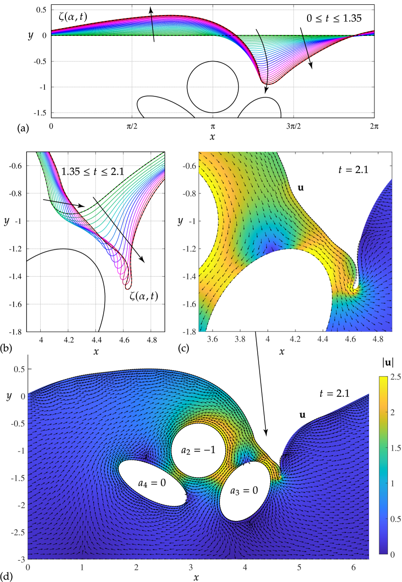
Figure 2: Evolution of the free surface and plots of the fluid velocity at the final time computed, $t=2.1$, for problem 1 of (7.2). The computation breaks down when evolved beyond $t=2.1$ with macro-steps of size $\Delta t=0.025$, but is on track to self-intersect in a splash singularity. The fluid is stagnant below the cylinders and the flow is reversed in the channels between cylinder 2 and its neighbors. As a result, the change in velocity potential across the domain is 0 or $2\pi$ depending on whether the path passes below or above cylinder 2.

In Figure 2, the clockwise circulation around cylinder 2 (due to $a_{2}=-1$) pulls the free surface down to the right of the cylinder, toward the channel between cylinders 2 and 3. This causes an upwelling to the left of cylinder 2 in order to conserve mass. At $t=1.35$, we see in panel (b) that the lowest point on the free surface stops approaching the channel and begins to drift to the right, around cylinder 3. The left (upstream) side of the interface (relative to its lowest point) accelerates faster than the right side, which causes the interface to sharpen and fold over itself. Shortly after $t=2.1$, our numerical solution loses resolution as the left side of the interface crashes into the right side to form a splash singularity castro2013finite ; castro2012splash . The colormap of the contour plot in panel (c) is the same as in panel (d). We see that the velocity is largest in magnitude in the region above and to the right of cylinders 2 and 3, and is relatively small throughout the fluid otherwise. The change in velocity potential along a path crossing the domain below all three cylinders is zero in this case since $V_{1}+a_{2}+a_{3}+a_{4}=0$, whereas the change along a path crossing above the cylinders is $2\pi$.

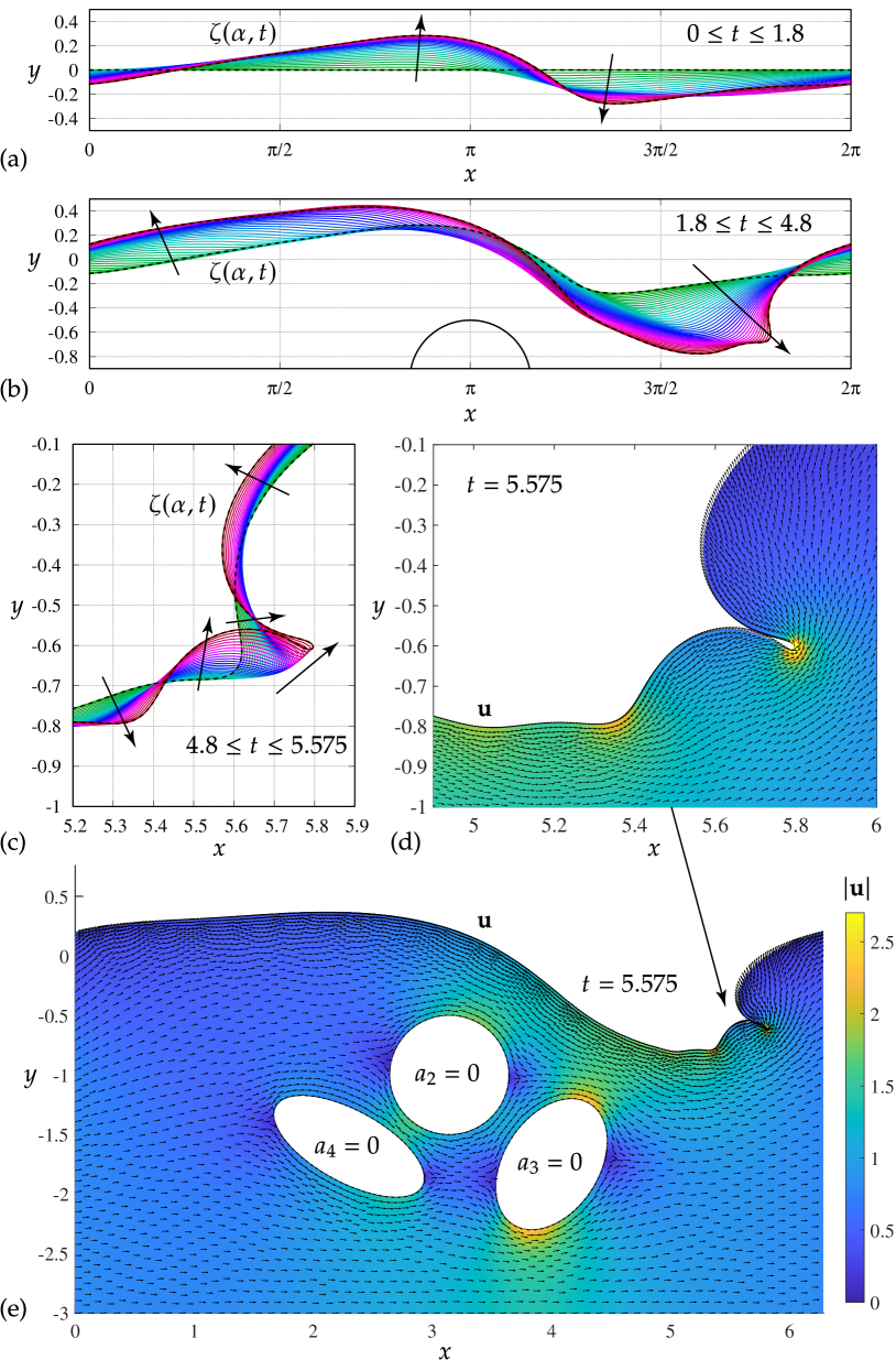
Figure 3: Evolution of the free surface and plots of the fluid velocity at the final time computed, $t=5.575$, for problem 2 of (7.2). The interface is on track to self-intersect in a splash singularity shortly after this, as is evident in panel (c). The velocity field in panel (d) on the upper surface of the air pocket is nearly tangential, whereas it has an appreciable normal component on the lower surface. This provides further evidence that a splash singularity is imminent.

In Figure 3, $a_{2}$ is set to zero, which causes the change in velocity potential along any path across the domain to be $2\pi$, whether it passes above, below or between the cylinders. As a result, the magnitude of velocity is more evenly spread throughout the fluid. This magnitude is largest below cylinder 3 and above cylinders 2 and 3, where the width of the fluid domain is smallest. Similar to problem 1, the free surface initially drops to the right of the cylinders and rises to the left, but it does not get pulled toward the channel between cylinders 2 and 3 since the flow is not reversed there this time. Nevertheless, the free surface eventually folds over itself, but farther downstream and at a later time than in problem 1. Panel (b) shows the development of an air pocket expanding into the fluid as it travels down and to the right. This air pocket sharpens in panel (c) to form a splash singularity shortly after $t=5.575$.

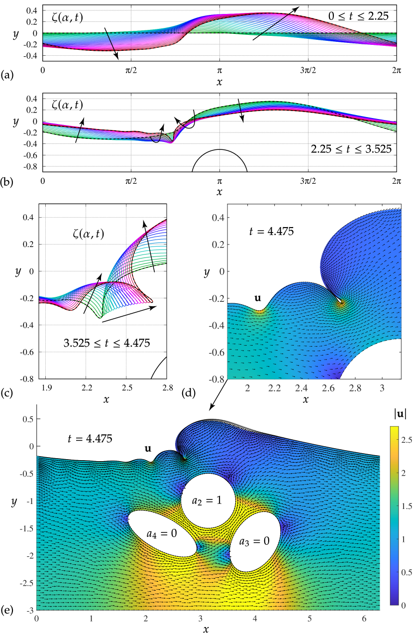
Figure 4: Evolution of the free surface and plots of the fluid velocity for problem 3 at $t=4.475$, when the stream function on the rigid boundaries is $\psi|_{1}=0$, $\psi|_{3}=2.243$, $\psi|_{4}=2.580$ and $\psi|_{2}=3.387$, and the fluid flux in the channels is $(\psi|_{2}-\psi|_{4})=0.807$ and $(\psi|_{2}-\psi|_{3})=1.144$.

In Figure 4, $a_{2}$ is set to 1. The counter-clockwise circulation around cylinder 2 causes the change in velocity potential to be $2\pi$ along a path crossing the domain above all three cylinders and to be $4\pi$ along a path passing below any subset of the cylinders that includes cylinder 2. The magnitude of velocity is largest in the channels between cylinder 2 and its neighbors, and below all three cylinders. The net flux below cylinder 3 is still larger than that passing between cylinders 2 and 3, as noted in the caption. There is an upwelling of the free surface above and to the right of cylinder 2 with a drop in fluid height to the left of the cylinders, which is the opposite of what happens in problems 1 and 2. Capillary waves form at the free surface ahead of the cylinders, with the largest oscillation eventually folding over to form a splash singularity. In the final stages of this process, shown in panel (c), a structure resembling a Crapper wave crapper ; akers2014gravity forms, which travels slowly to the right as the fluid flows faster around and below it (left to right). As it evolves, the sides of this structure slowly approach each other while also slowly rotating counter-clockwise.

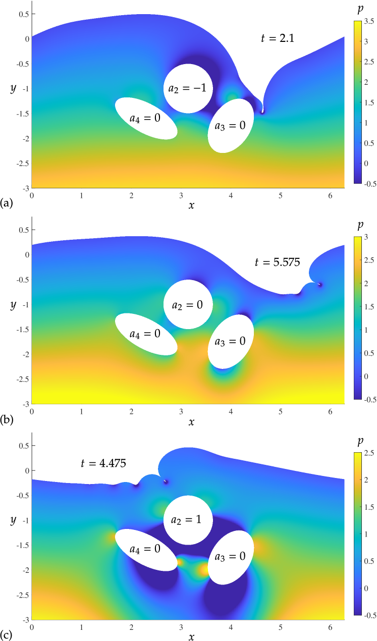
Figure 5: Pressure in the fluid at the final times computed for problems 1–3 of (7.2).

Figure 5 shows the pressure in the fluid at the final times shown in Figures 2–4. On the free surface, the pressure is given by the Laplace-Young condition, $p=p_{0}-\rho\tau\kappa$, where we take $p_{0}=0$, $\rho=1$ and $\tau=0.1$. Setting $p_{0}=0$ means pressure is measured relative to the ambient pressure, so negative pressure is allowed. The curvature $\kappa=\theta_{\alpha}/s_{\alpha}$ is positive when the interface curves to the left (away from the fluid domain) as $\alpha$ increases, i.e., moving along the interface from left to right. Inside the fluid, we compute $p$ using (5.4) and (5.8), as explained in Section 5.1 above. From (5.4), we see that pressure increases with fluid depth and decreases in regions of high velocity, up to the correction $\phi_{t}$ in (5.4), which is a harmonic function satisfying homogeneous Neumann boundary conditions on the solid boundaries.

In all three panels of Figure 5, the pressure is visibly lower near the capillary wave troughs, especially the largest trough that folds over into a structure similar to a Crapper wave before the splash singularity forms. As the circulation parameter $a_{2}$ increases from $-1$ in panel (a) to 0 in panel (b) and to 1 in panel (c), the pressure decreases near the bottom boundary. Problem 3 has higher velocities than problems 1 and 2 below the cylinders and in the channels between cylinders, which leads to smaller pressures in these regions in panel (c) than in panels (a) and (b). This effect would have been even more evident if we had used the same colorbar scaling in all three plots, but this would have washed out some of the features of the plots.

The contour plots of Figures 2-4 confirm that the fluid velocity increases in the neighborhood of the capillary wave troughs (where the pressure is lower), and is quite large below the Crapper wave structure. We also see in Figure 5 that in problem 1, which involves negative circulation around the top-most body, the pressure above this obstacle is significantly lower than elsewhere. This sheds light on an effect observed experimentally wu1972cavity whereby an air bubble can be permanently trapped between the top of an airfoil and the free surface. We will investigate this phenomenon in more detail in future work.

7.2 Free-surface flow in a geometry with variable bottom topography

Next we consider an example (problem 4) in which the bottom boundary drops off rapidly and later rises again, forming a basin in between. We define $\zeta_{1}(\alpha)=\alpha+i\eta_{1}(\alpha)$ with $\eta_{1}(\alpha)$ satisfying

$$\eta_{1}(0)=-\frac{1}{2},\qquad\eta_{1}^{\prime}(\alpha)=-5\sin^{63}\alpha,\qquad 0\leq\alpha\leq 2\pi.$$ (7.3)

The 63rd power of $\sin(\alpha)$ is close to zero except near $\alpha=\frac{\pi}{2}$ and $\alpha=\frac{3\pi}{2}$, causing $\eta_{1}(\alpha)$ to be quite flat in both the shallow and deep regions. The fluid depth ranges from $\eta_{1}(0)=-0.5$ to $\eta_{1}(\pi)=-2.072774$, and is $2\pi$-periodic since $\sin^{63}\alpha$ has zero mean. We place a large ellipse in the center of the basin to create a channel between the ellipse and the bottom boundary boundary. We force some of the fluid to flow through the channel by setting $a_{2}=1/2$. We place a smaller ellipse near the entrance of the channel and set the circulation parameter of this ellipse to be $a_{3}=0$. In the notation of (7.1), the ellipse positions, sizes and circulation parameters are given by

$$\begin{array}[]{|c|c|c|c|c|c|r|}\hline\cr\vrule\lx@intercol\hfil\text{Obstacle data in problem 4}\hfil\lx@intercol\vrule\lx@intercol\\ \hline\cr\quad j&\quad x_{j}&\quad y_{j}&\quad q_{j}&\quad b_{j}&\quad\theta_{j}&\quad a_{j}\\[2.0pt] \hline\cr\quad 2&\quad\pi&\quad-9/8&\quad 4/3&\quad 3/4&\quad 0.0&\quad 0.5\\ \quad 3&\quad 1.8&\quad-0.4&\quad 0.2&\quad 0.1&\quad 0.0&\quad 0.0\\ \hline\cr\end{array}$$ (7.4)

As in Section 7.1, we also set $V_{1}=1$, $\tau=0.1$ and $g=1$.

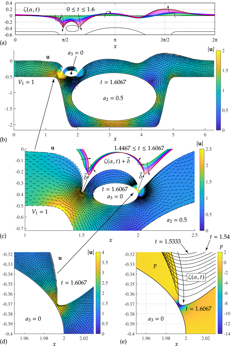
Figure 6: Time evolution of the free surface and plots of velocity and pressure at $t=1.6067$. The time increments shown in panels (a), (c) and (e) are $0.08$, $0.01333$ and $0.00667$, respectively. In panel (c), an offset $\vec{\delta}=(0.06,0.15)$ was added to the free surface plots to avoid obscuring the contour plot. In panel (e), the free surface approaches the obstacle at an accelerating rate as the gap shrinks and the curvature of the free surface grows. The numerical solution is still resolved with spectral accuracy at $t=1.6067$, but we cannot not proceed without further mesh refinement.

In Figure 6, panel (a) shows the time evolution of the free surface for $0\leq t\leq 1.6$, computed using the velocity potential method. The curves are shown at equal time intervals of size $\Delta t=0.08$. They are color coded to evolve from green to blue to red in the direction of the arrows. The interface is initially flat and the periodic part of the velocity potential is initially set to zero, $\tilde{\varphi}(\alpha,0)=0$. Setting $V_{1}=1$, $a_{2}=1/2$ and $a_{3}=0$ causes the fluid entering the domain from the left to split into two parts, one flowing down through the channel between the basin and the large ellipse and the other flowing above the large ellipse from left to right. This leads to a stagnation point in the upper left quadrant of the large ellipse, as shown in panel (b) at $t=1.6067$. A similar stagnation point is present in the upper right quadrant, where the two streams recombine to flow over the right edge of the basin. This leads to an upwelling of fluid above the right edge of the basin, as shown in panels (a) and (b). The opposite occurs at the left edge of the basin, where the free surface is pulled down by the fluid entering the channel below. The presence of the small obstacle causes the free surface to form two air pockets moving downward on either side of the obstacle. We exclude arrows in the velocity direction field near these air pockets in panel (b) to avoid obscuring the contour plots.

Panel (c) of Figure 6 provides a magnified view of the flow near the small obstacle, including the direction field near the upstream air pocket (to the left of the obstacle). The contour plot and direction field correspond to $t=1.6067$. We also show the time evolution of the free surface leading up to this state, with $t$ ranging from $1.44667$ to $1.60667$, plotted at time increments of $0.01333$. We plot $\zeta(\alpha,t)+\vec{\delta}$, where we have introduced the offset $\vec{\delta}=(0.06,0.15)$ to separate the evolving curves from the contour plot. As time evolves, each of the air pockets sharpens as it is pulled further into the fluid. The upstream air pocket begins to form a Crapper-wave structure similar to those seen in Figures 2–5 in Section 7.1, and would likely form a splash singularity at a later time. But before this happens, the right air pocket approaches the obstacle and appears on track to collide with it shortly after $t=1.6067$.

Panel (d) of Figure 6 shows the magnitude and direction of the velocity in the neighborhood of the point of closest approach at $t=1.6067$. The fluid moves fastest in the small gap between the free surface and the obstacle. The increased speed is caused by a large pressure drop in the gap, shown in panel (e), which causes the fluid to accelerate as it approaches the gap and decelerate afterwards. The pressure drop is caused by surface tension and the high curvature of the interface near the gap. Also shown in panel (e) are snapshots of the interface from $t=1.53333$ to $t=1.60667$ in increments of $\Delta t=0.00667$. These curves are plotted in black since the direction of motion is clear. The free surface appears to approach the obstacle at an accelerating rate as it sharpens. We believe an impact will occur with a simultaneous blow-up of the curvature there, though it is possible that the interface will slide around the obstacle before crashing into it or crash into it before forming a curvature singularity. Further investigation would likely require using a non-uniform grid (rather than arclength parameterization) and adapting the ideas of Appendix F to handle the close approach of the interface to the obstacle without excessive mesh refinement; however, these are topics for future research.

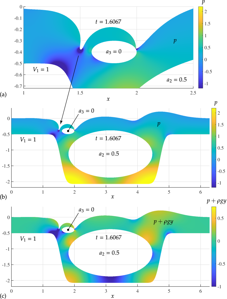
Figure 7: The pressure is lowest where the free surface has high curvature and where the fluid velocity is highest, e.g., due to flowing through a constriction. The hydrostatic term $-\rho gy$ in (5.4) is responsible for the high-pressure regions in the bottom corners of the basin in panel (b). This term has been eliminated by adding $\rho gy$ to $p$ in panel (c).

Zooming out from panel (e) of Figure 6 and rescaling the colorbar yields the pressure plot (at $t=1.6067$) shown in panel (a) of Figure 7. Comparison with panel (c) of Figure 6 shows that the pressure is lowest where the velocity is highest, with local minima occurring under the two air pockets of the free surface, at the left edge of the basin where the bottom boundary drops off, and along part of the lower-left boundary of the small obstacle. Zooming out further to the entire domain gives the pressure plot in panel (b). The scaling of the colorbar is the same as in panel (a). Here the effects of the hydrostatic term $-\rho gy$ in the formula (5.4) for $p$ are clearly seen, with the largest values of pressure occurring in the bottom corners of the basin. In panel (c) we plot the deviation from this hydrostatic state, which would be the equilibrium pressure if the fluid were at rest with a flat free surface. We see a large negative deviation where the fluid flows fastest and where the free surface curves upward most rapidly, and positive deviations near the stagnation points on the large obstacle, in the bottom corners of the basin, and in the upwelling above the right edge of the basin.

$$\begin{array}[]{r|c|c|c|c|c|c|c}M_{0}&\;768&\;1536&\;3072&\;5184&\;9216&\;12288&\;16384\\ M_{3}&\;256&\;256&\;256&\;288&\;768&\;1296&\;1536\\ \hline\cr d&8&20&50&90&210&300&450\\ \hline\cr ns&138&48&30&18&6&2/3&1/3\\ \hline\cr\text{GEPP}(\tilde{\varphi})&2.80&13.7&77.2&370&3103&9605&29184\\ \text{GEPP}(\gamma_{0})&4.14&17.1&97.7&419&3734&10779&35437\\ \text{GMRES}(\tilde{\varphi})&1.98&9.07&59.6&260&2019&6278&15925\\ \text{GMRES}(\gamma_{0})&3.25&13.8&93.1&334&2831&9897&27921\\ \text{GMRES}(\text{GPU},\tilde{\varphi})&0.62&2.37&12.6&48.7&364&937&2492\end{array}$$

Table 3: Parameters used to timestep problem 4 from the initial flat state to a near collision of the free surface with an obstacle. We set $M_{1}=768$ and $M_{2}=M_{3}$ in each case. Here $d$ and $ns$ have the same meanings as in Table 2, except that the macro-step size is $\Delta t=0.00667$ instead of $0.025$. The fractional steps with $ns=2/3$ and $1/3$ indicate a change in mesh size part-way through the final macro-step from $t=1.6$ to $1.60667$, shown in panel (e) of Figure 6. The last 5 rows report the wall-clock running time (in seconds) of one macro-step for the solvers we implemented.

We used the sequence of meshes and stepsizes listed in Table 3 to evolve the solution with spectral accuracy from $t=0$ to $t=1.6067$, the time at which the velocity and pressure are plotted in Figures 6 and 7. In all cases, we discretize the bottom boundary with $M_{1}=768$ points and set $M_{2}=M_{3}$ for the two obstacles. $M_{3}$ must increase as the interface approaches the small obstacle in order to maintain spectral accuracy in the Fourier representation of $\omega_{3}(\alpha,t)$. It would have been sufficient to use $M_{2}=256$ throughout the computation since the free surface does not approach the large obstacle; however, for simplicity, our code assumes each obstacle has the same number of gridpoints. In the terminology of Table 2, we have set the macro-step size to $\Delta t=0.00667$. This is the temporal spacing of the curves plotted in panel (e) of Figure 6. The curves in panels (a) and (c) were plotted with time increments of $0.08$ and $0.01333$, which are every 12th and every 2nd macro-step, respectively.

In each column of Table 3, $ns$ macro-steps were taken with the listed values of $M_{0}$, $M_{3}$ and $d$, where $d$ is the number of Runge-Kutta steps per macro-step. The last 5 rows report the wall-clock running time (in seconds) of evolving the solution through one macro-step using the velocity potential or vortex sheet method with Gaussian elimination or GMRES to solve the linear systems that arise. We also implemented a GPU-accelerated version of the GMRES solver in the velocity potential framework. The final macro-step to evolve the solution from $t=1.60000$ to $t=1.60667$ was done in two stages with the parameters listed in the last two columns of the table. Both $d$ and the running times are scaled in the table to correspond to one full macro-step. Multiplication by $ns$ gives the total number of Runge-Kutta steps and the total computational time of that phase of the numerical solution. The running times of the solvers we tested will be discussed further in Section 7.4 below.

7.3 Fourier mode decay, energy conservation and comparison of results

In this section we compare the numerical results of the velocity potential and vortex sheet formulations for the test problems (7.2). Since we have taken the single-valued part of the surface velocity potential to be zero initially, i.e., $\tilde{\varphi}(\alpha,0)=0$, we have to compute the corresponding initial vortex sheet strength $\gamma_{0}(\alpha,0)$ to solve an equivalent problem using the vortex sheet formulation. This is easily done within the velocity potential code by first computing $\omega_{j}(\alpha,0)$ by solving (3.13) and then evaluating $\gamma_{0}(\alpha,0)=-\omega_{0}^{\prime}(\alpha,0)$ in (4.1). Because $V_{1}$ and possibly $a_{2}$ are nonzero, this initial condition $\gamma_{0}(\alpha,0)$ is nonzero for each of the three problems (7.2).

Figure 8 shows the Fourier mode amplitudes of $\theta(\alpha,t)$ and $\varphi_{0}(\alpha,t)$ or $\gamma_{0}(\alpha,t)$ for problem 3 at the final time computed, $t=4.475$. The results are similar for problems 1 and 2 at $t=2.1$ and $t=5.575$, respectively, so we omit them. At $t=4.475$ in problem 3, there are $M_{0}=7776$ gridpoints on the free surface, so the Fourier mode index ranges from $k=0$ to $3888$. We only plotted every fifth data point (with $k$ divisible by 5) so that individual markers can be distinguished from one another. The blue and black markers show the results of the velocity potential and vortex sheet formulations, respectively. In both formulations, the Fourier modes decay to $10^{-12}$ before a rapid drop-off due to the Fourier filter occurs. Beyond $k=2500$, the Fourier modes of the velocity potential formulation begin to look noisy and scattered, which suggests that roundoff errors are having an effect. This is not seen in the vortex sheet formulation. A possible explanation is that because $\widehat{\varphi_{0}}_{k}$ decays faster than $\widehat{\gamma_{0}}_{k}$, there is some loss of information in storing $\varphi_{0}(\alpha,t)$ in double-precision to represent the state of the system relative to storing $\gamma_{0}(\alpha,t)$. Indeed, combining (3.20), (3.22) and (3.27) in the velocity potential formulation gives the same formula (4.8) for the normal velocity $U$ in the vortex sheet formulation, but we have to solve for the $\omega_{j}$ and then differentiate these to obtain the $\gamma_{j}$ before computing $U$ in the velocity potential formulation.

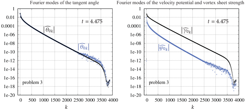
Figure 8: Fourier mode amplitudes of $\theta_{0}(\alpha,t)$ and $\varphi_{0}(\alpha,t)$ or $\gamma_{0}(\alpha,t)$ for problem 3 of (7.2) at $t=4.475$, computed using the velocity potential (blue) or vortex sheet (black) formulations.

This is not a complete explanation for the smoother decay of $\widehat{\gamma_{0}}_{k}$ as the right-hand sides of (4.14) and (4.17), which govern $\gamma_{j,t}(\alpha,t)$, contain an extra $\alpha$-derivative relative to the right-hand side of (3.30) for $\tilde{\varphi}_{t}(\alpha,t)$. But it appears that the dispersive nature of the evolution equations and the Fourier filter suppress roundoff noise caused by this $\alpha$-derivative. We emphasize that the smoother decay of Fourier modes in the vortex sheet formulation does not necessarily mean that these results are more accurate than the velocity potential approach. The $\alpha$-derivatives in the right-hand sides of (4.14) and (4.17) may cause just as much error as arises in computing $\gamma_{j}(\alpha,t)$ from $\tilde{\varphi}_{0}$, but it is smoothed out more effectively in Fourier space for the vortex sheet formulation. A higher-precision numerical implementation would be needed to investigate the accuracy of each method independently, which is beyond the scope of the present work.

In Figure 9, we plot the norm of the difference of the numerical solutions obtained from the velocity potential and vortex sheet formulations for problem 1 (left) and problems 2 and 3 (right). Since the tangent angle $\theta(\alpha,t)$ is computed directly in both formulations, we use

$$\text{err}_{1}(t)=\sqrt{\frac{1}{2\pi}\int_{0}^{2\pi}|\theta_{\text{vp}}(\alpha,t)-\theta_{\text{vs}}(\alpha,t)|^{2}\,d\alpha}$$ (7.5)

as a measure of the discrepancy between the two calculations, where vp and vs refer to ‘velocity potential’ and ‘vortex sheet.’ The results are plotted in blue, green and red for problems 1, 2 and 3, respectively. In all three cases, $\text{err}_{1}(t)$ grows exponentially in time from the initial flat state to the final time computed, just before the splash singularity would occur. This exponential growth is likely due to nearby solutions of the water wave equations diverging from one another with an exponential growth rate with this configuration of obstacles, background flow, and circulation parameters $a_{j}$. We do not believe the exponential growth is due to numerical instabilities in the method beyond those associated with dynamically increasing the number of mesh points, $M_{0}$, and timesteps, $d$, per time increment plotted, $\Delta t=0.025$, as listed in Table 2. At the final time, $\text{err}_{1}(t)$ has only grown to around $10^{-9}$ in spite of the rapid change in $\theta(\alpha,t)$ by $2\pi$ radians over a short range of $\alpha$ values when traversing the structures resembling Crapper waves in Figures 2–5.

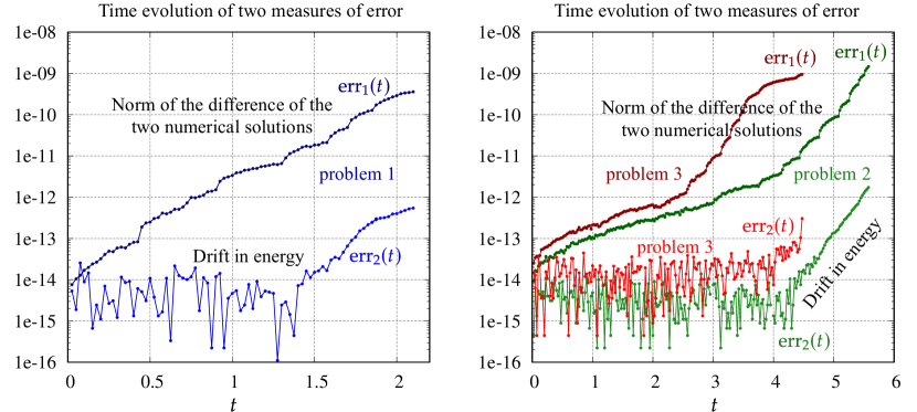
Figure 9: Time evolution of $\text{err}_{1}(t)$ and $\text{err}_{2}(t)$ from (7.5) and (7.6) for problems 1, 2 and 3 from the initial flat state to the final time computed for each problem, just before the splash singularity.

As a second measure of error, we also plot in Figure 9 the change in energy from the initial value,

$$\text{err}_{2}(t)=E(t)-E(0),$$ (7.6)

for all three problems, shown in lighter shades of blue, green and red. In each numerical calculation, this change in energy remains in the range $10^{-16}$–$10^{-14}$ for early and intermediate times. For comparison, the values of $E(0)$ are

$$\begin{array}[]{r|ccc}\text{problem}&1&2&3\\ \hline\cr\raisebox{-1.0pt}{$E(0)$}&\;\raisebox{-1.0pt}{$0.79004$}&\;\raisebox{-1.0pt}{$1.29626$}&\;\raisebox{-1.0pt}{$3.71426$}\end{array}$$ (7.7)

At later times, $\text{err}_{2}(t)$ begins to grow exponentially at a rate similar to that of $\text{err}_{1}(t)$ but remains 3–4 orders of magnitude smaller. Thus, while energy conservation is a necessary condition for maintaining accuracy, it tends to under-predict the error of a numerical simulation.

7.4 Running time and performance

The wall-clock times listed in Tables 2 and 3 above were obtained by running our C++ implementation of the velocity potential and vortex sheet methods with 24 OpenMP threads on a server with two 12-core 3.0 GHz Intel Xeon Gold 6136 processors. The rows labeled GEPP$(\tilde{\varphi})$ or GEPP$(\gamma_{0})$ in the tables correspond to using Gaussian elimination with partial pivoting to solve (3.18) in the velocity potential method or (4.5), (4.14) and (4.17) in the vortex sheet method. The rows labeled GMRES$(\tilde{\varphi})$ or GMRES$(\gamma_{0})$ correspond to using the generalized minimal residual method golub:book to solve these linear systems.

We also implemented a version of the GMRES code in which the matrix entries of these linear systems are computed and stored on a graphics processing unit (GPU) and the matrix-vector multiplications of the GMRES algorithm are performed on the GPU. This approach is effective as $O(M^{2}i_{\text{max}})$ work is done on the GPU for each linear system solved, with only $O(M\,i_{\text{max}})$ communication cost between the CPU and GPU, where

$$M=M_{0}+M_{1}+\cdots M_{N}$$ (7.8)

is the size of the linear systems (3.18), (4.14) and (4.17) and $i_{\text{max}}$ is the number of GMRES iterations required for convergence (typically 30–120, as discussed below). This part of the code was written in Cuda and run on the same server, which has an Nvidia Tesla P100-PCIE-16GB GPU with 3584 cores running at 1.2 GHz. Less expensive operations such reconstructing $\zeta(\alpha,t)$ from $P\theta(\alpha,t)$, computing $\alpha$-derivatives, and applying the Fourier filter (5.2) at the end of each Runge-Kutta step are still done on the CPU.

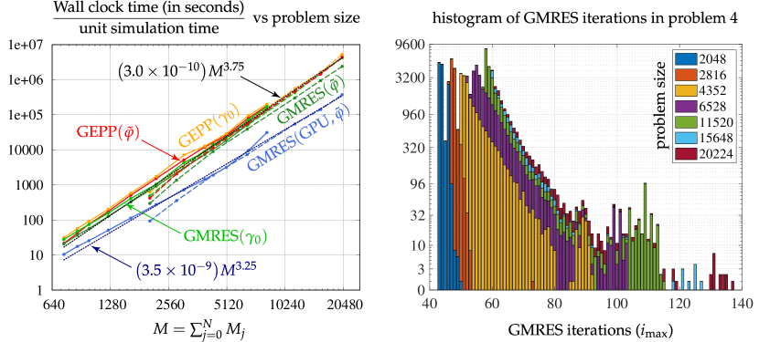
Figure 10: Wall-clock running time per unit simulation time versus problem size for the velocity potential $(\tilde{\varphi})$ and vortex sheet $(\gamma_{0})$ formulations using Gaussian elimination (GEPP) or GMRES to solve the linear systems that arise in problems 1–3 and 4, and histogram of the number of GMRES iterations required to achieve convergence in problem 4.

The performance results are plotted on a log-log plot in the left panel of Figure 10. Since problem 4 has a different macro-step size $\Delta t$ from problems 1–3, we divided the wall-clock running times by $\Delta t$ to obtain the wall-clock time per unit simulation time as a function of problem size, $M$. The bottom 5 rows of Table 2 are plotted with solid lines that extend from $M=736$ to $8256$ while the bottom 5 rows of Table 3 are plotted with dashed lines that extend from $M=2048$ to $20224$. The orange and light green curves show the GEPP and GMRES results for the vortex sheet method, respectively, while the red and dark green curves show the GEPP and GMRES results for the velocity potential method. The blue curves show the results of the GPU-accelerated GMRES code for the velocity potential method. We did not implement the GPU variant of the GMRES algorithm in the vortex sheet framework.

We find that the wall-clock running time of the GEPP algorithm scales like $O(M^{3.75})$ at the larger grid sizes used in problem 4. This is demonstrated with the dotted black line in the left panel of Figure 10. One expects $O(M^{4.5})$ scaling, with a factor of $O(M^{3})$ from the cost of Gaussian elimination and a factor of $d$ from Tables 2 and 3, the number of Runge-Kutta steps taken per macro-step of fixed size $\Delta t$. A small-scale decomposition analysis HLS1 ; HLS2 shows that the surface tension terms in (3.30) and (4.14) make the systems mildly stiff, and $d$ should grow like $O(M_{0}^{3/2})$ to maintain stability using an explicit Runge-Kutta method. Since $M_{0}\geq(3/8)M$ in all cases considered here, this gives an $O(M^{4.5})$ growth rate. But the linear algebra runs more efficiently on a multi-core CPU for larger problem sizes, which reduces the wall-clock running time to $O(M^{3.75})$ in this test problem. This modest reduction does not change the fact that the method becomes expensive far large grid sizes. For example, the total running time of the GEPP solver for problem 4 was 12.4 hours in the velocity potential framework and 14.8 hours in the vortex sheet framework, and 36% of this time was devoted in each case to evolving the solution through the final macro-step via the last two columns of Table 3.

Switching to GMRES eliminates the $O(M^{3})$ operations of the LU-factorization but requires several matrix-vector multiplications to be performed iteratively, each costing $O(M^{2})$ operations. We denote the number of iterations required to reduce the norm of the residual to $10^{-15}$ times the norm of the right-hand side by $i_{\text{max}}$. There is still a factor of $d$, which scales like $O(M^{3/2})$, so the expected running time is $O(M^{3.5}i_{\text{max}})$. As with GEPP on the CPU, the GPU makes more efficient use of its many cores for larger problem sizes. Thus, even though $i_{\text{max}}$ grows somewhat with $M$, as discussed below, we find that the wall-clock running time scales like $O(M^{3.25})$, shown by the dotted navy line in the left panel of Figure 10. Instead of 12.4 hours, the running time of problem 4 drops to 1.4 hours using the GPU in the velocity potential framework, with 28.6% of the time devoted to the final macro-step.

Next we investigate how the number of GMRES iterations needed for convergence, $i_{\text{max}}$, depends on $M$. A benefit of discretizing second-kind integral equations is that the condition number remains $O(1)$ as the mesh size approaches zero. But in the current case, the mesh is refined in response to the domain evolving toward increasingly complicated geometries, which affects the condition number. The right panel of Figure 10 shows a histogram of the resulting $i_{\text{max}}$ for each of the linear systems solved during the course of evolving problem 4 in the velocity potential framework. Each column of Table 3 corresponds to a batch of Runge-Kutta steps with a fixed value of $M$. Each of these Runge-Kutta steps contributes 12 values of $i_{\text{max}}$ to the histogram (as it is a 12-stage, 8th order scheme), and there are a handful of additional $i_{\text{max}}$ values in the histogram from computing the energy at the output times.

We color-code the histogram results by problem size. We see that colors corresponding to larger problem sizes occupy bins further to the right in the histogram, which means that as the free surface evolves to a more complicated state and requires more gridpoints, the number of GMRES iterations also increases. But the change is not drastic. Tables 4 and 5 give the average value of $i_{\text{max}}$ for each linear system with a given problem size $M$ that arises in problems 3 and 4, where problem 3 is representative of problems 1–3, which have the same grid parameters. We see in Table 5, for example, in the velocity potential framework, that increasing $M$ from 2048 to 20224 in problem 4 causes the average value of $i_{\text{max}}$ to increase from $43.0$ to only $70.0$.

$$\begin{array}[]{r|c|c|c|c|c|c|c|c|c|c|c}M&\;736&\;864&\;992&\;1248&\;1632&\;2208&\;3072&\;3936&\;5088&\;6624&\;8256\\ \hline\cr\text{restart parameter}&50&50&50&50&50&50&50&60&60&70&90\\ \hline\cr\text{average }i_{\text{max}}(\tilde{\varphi})&31.6&34.0&34.7&35.1&36.2&37.2&39.0&40.0&41.0&47.2&66.5\\ \text{average }i_{\text{max}}(\gamma_{0})&33.2&35.6&36.2&36.6&37.5&38.2&39.1&40.1&42.2&47.1&67.9\\ \hline\cr\text{\% restarted}(\tilde{\varphi})&0&0&0&0&0&0&0&0&0&0.10&0.50\\ \text{\% restarted}(\gamma_{0})&\,0.017&\,0.092&0&0.020&0&0&0&0&0.749&0&3.97\\ \hline\cr\text{avg. }i_{\text{max}}(\gamma_{0};\text{aux})&20&20&20&20&20&20&20&20&20&20&20.6\\ \text{\% restarted}(\gamma_{0};\text{aux})&0&0&0&0&0&0&0&0&0&0&0\end{array}$$

Table 4: GMRES performance in problem 3. The rows labeled $i_{\text{max}}$ give the average number of GMRES iterations required for convergence. Also shown are the percentage of cases in which GMRES was restarted due to the iteration count reaching the restart parameter. The rows labeled “aux” refer to the auxiliary linear system (4.5) of the vortex sheet formulation.

$$\begin{array}[]{r|c|c|c|c|c|c|c}M&\;2048&\;2816&\;4352&\;6528&\;11520&\;15648&\;20224\\ \hline\cr\text{restart parameter}&60&70&80&90&100&110&120\\ \hline\cr\text{average }i_{\text{max}}(\tilde{\varphi})&43.0&46.9&53.2&59.1&62.7&63.6&70.0\\ \text{average }i_{\text{max}}(\gamma_{0})&63.0&52.5&56.4&57.2&59.7&105&116\\ \hline\cr\text{\% restarted}(\tilde{\varphi})&0&\,0.0087&0.54&0.68&2.0&0.42&0.88\\ \text{\% restarted}(\gamma_{0})&72&2.4&6.0&0.18&0.59&63&66\\ \hline\cr\text{avg. }i_{\text{max}}(\gamma_{0};\text{aux})&26.4&26.4&26.3&26.4&27.0&27.2&27.4\\ \text{\% restarted}(\gamma_{0};\text{aux})&0&0&0&0&0&0&0\end{array}$$

Table 5: GMRES performance in problem 4. Each column corresponds to a batch of Runge-Kutta steps with a fixed spatial discretization. In the first column and last two columns, a large fraction of the linear systems in the vortex sheet formulation stall on the first GMRES cycle, but then converge rapidly after a single restart. This causes the average $i_{\text{max}}$ to be 45–65% larger in the vortex sheet framework than the velocity potential framework in these columns.

Also listed in Tables 4 and 5 are the GMRES restart parameters used, as well as the percentage of linear systems of each problem size in which the iteration count reached the restart parameter before the convergence criterion was reached, triggering a restart. In problem 3, this was rare, occurring less that 1% of the time in all cases except $M=8256$ with the vortex sheet method, when it occurred just under 4% of the time. But in problem 4, while still rare for the velocity potential method, it was common for GMRES to stall in the first cycle of iterations and then converge rapidly after a single restart. As seen in Table 5, this occurred 72% of the time with $M=2048$, 63% of the time with $M=15648$, and 66% of the time with $M=20224$. In these cases, we find that increasing the restart parameter has a negative impact on performance as the extra iterations of the first GMRES cycle are not as effective at reducing the residual as they would have been had a restart already occurred. But we also find that reducing the restart parameter to a small value like 10 or 12 does not work well as the number of restart cycles can then increase significantly. With the restart parameters listed in Table 4 and 5, convergence was always reached with at most one restart in all cases encountered. For background on selecting optimal restart parameters in GMRES, see baker:gmres:restart .

In the vortex sheet approach, one also has to solve the auxiliary linear system (4.5) for $\gamma_{1}$, …, $\gamma_{N}$. This system only involves discretization points on the solid boundaries, which do not become more geometrically complicated as the free surface evolves. We find that the value of $i_{\text{max}}$ for this auxiliary system is extremely stable, taking on the value of 20 or 21 for all 58671 linear systems that arose in timestepping problem 3, independent of $M$ in (7.8), and ranging between 26 and 32 in all cases that arose in timestepping problem 4, with the average value increasing from 26.4 to 27.4 as $M$ changes from 2048 to 20224. There were no instances of a restart occurring for the auxiliary problem in problems 3 or 4.

$$\begin{array}[]{r|c|c|c|c||c|c|c|c||c|c|c|c}\text{solver}&\vrule\lx@intercol\hfil GEPP\hfil\lx@intercol\vrule\lx@intercol\vrule\lx@intercol&\vrule\lx@intercol\hfil GMRES\hfil\lx@intercol\vrule\lx@intercol\vrule\lx@intercol&\vrule\lx@intercol\hfil GMRES(GPU)\hfil\lx@intercol\\ \hline\cr\text{problem}&1&2&3&4&1&2&3&4&1&2&3&4\\ \hline\cr\text{total time}(\tilde{\varphi})&\,1.17&\,7.3&\,21.3&\,12.4&\,0.71&\,5.3&\,14.9&\,8.0&\,0.157&\,1.11&\,2.84&\,1.41\\ \hline\cr\text{\% increase}(\gamma_{0})&\,13.1&\,14.5&\,15.9&\,19.0&\,24&\,26&\,29&\,49&\,-&\,-&\,-&\,-\end{array}$$

Table 6: Total running times (in hours) of the velocity potential method on problems 1–4 with the solvers implemented and the percentage increase in running time of the vortex sheet method.

We find that the vortex sheet method takes 13–50% longer to solve problems 1–4 when implemented using the same solver. Table 6 gives the total running times (in hours) of the velocity potential method and the percentage increase in running time of the vortex sheet method. With Gaussian elimination, the discrepancy is due to having to solve the auxiliary problem (4.5) in addition to the system (4.14) and (4.17). The latter system is computationally equivalent to the system (3.18) in the velocity potential method. However, the auxiliary problem is smaller (of size $M-M_{0}=M_{1}+\cdots+M_{N}$), adding 13–19% rather than doubling the running time in problems 1–4. With GMRES, the performance is somewhat worse, ranging from 24–29% slower in problems 1–3 and 49% slower in problem 4. This is partly due to the additional cost of the auxiliary problem, and also due to a larger average number of GMRES iterations being needed in the vortex sheet method, especially in problem 4, as noted in Table 5.

We remark that $d$ can be reduced to $O(M)$ via the HLS small-scale decomposition HLS1 ; HLS2 using an implicit-explicit Runge-Kutta scheme carpenter or exponential time-differencing scheme cox:matthews . The latter has been implemented in quasi:ivp , for example. But these are 4th or 5th order schemes, so there is a trade-off between the stability constraints of an 8th order explicit method and the accuracy constraints of an IMEX or ETD scheme. We did not explore this here, but it would impact the scaling of running time versus problem size in both the GEPP and GMRES approaches discussed above.

We also note that GMRES is faster than Gaussian elimination, though not by as much as one might predict from an operation count. While factoring the matrix requires $O(M^{3})$ operations, they run at level 3 BLAS speed. By contrast, GMRES requires $i_{\text{max}}$ matrix-vector multiplications to be computed sequentially, each involving $O(M^{2})$ operations that run at level 2 BLAS speed. For example, when $M=20224$ in problem 4, the average value of $i_{\text{tot}}$ was $70$, and the ratio of flops between GEPP and GMRES is roughly $(2M^{3}/3)/(70\times 2M^{2})\approx 96$, but the ratio of running times (from the last column of Table 3) is only $29184/15925=1.83$. Using the GPU improves this significantly to $29184/2492=11.7$. In future work, one could try switching to a block variant of GMRES baker:gmres:block , which might further improve the performance of the iterative approach by reducing the number of iterations and enabling much of the work to be done using level 3 BLAS routines. One could also explore the use of fast algorithms rokhlin85 ; nishimura02 to reduce the $O(M^{2})$ cost of forming the matrices and performing GMRES iterations, but the current approach is likely to remain competitive since it is easy to parallelize and could be run on a supercomputer for larger matrix sizes.

8 Conclusion

We presented two spectrally accurate numerical methods for computing the evolution of gravity-capillary water waves over obstacles and variable bottom topography. The methods are closely related, differing in whether the surface velocity potential or the vortex sheet strength is evolved on the free surface, along with its position. The kinematic variable governing the free surface position can be the graph-based wave height $\eta(x,t)$ or the tangent angle $\theta(\alpha,t)$ introduced by Hou, Lowengrub and Shelley. In the latter case, we showed how to modify the curve reconstruction by evolving only the projection $P\theta$ and using algebraic formulas to determine the mean value $P_{0}\theta$ and curve length $L=2\pi s_{\alpha}$ from $P\theta$. This prevents $O(\Delta t^{2})$ errors in internal Runge-Kutta stages from causing errors in high-frequency modes that do not cancel when the stages are combined into a full timestep. The bottom boundary and obstacles can be parameterized arbitrarily; we do not assume equal arclength parameterizations.

We derived an energy formula that avoids line integrals over branch cuts through the fluid by taking advantage of the existence of a single-valued stream function. This formula does not generalize to 3D, but also is not necessary in 3D since the velocity potential is single-valued in that case. We overcame a technical challenge in the velocity potential method by correcting a nontrivial kernel by modifying the equations to solve for the stream function values on the solid boundaries. This issue does not arise in the vortex sheet method unless the energy is being computed using the velocity potential approach. We also derived formulas for velocity and pressure in the fluid that retain spectral accuracy near the boundaries using a generalization of Helsing and Ojala’s method helsing to the periodic case. This method also is limited to 2D as it makes use of complex analysis through the Cauchy integral formula or the residue theorem. A different approach will need to be developed in 3D in future work.

The angle-arclength formulation is convenient for studying overturning waves, which we demonstrate in a geometry with three elliptical obstacles and another with two obstacles and a basin-shaped bottom boundary. In all cases, a flat initial interface develops one or more localized indentations that sharpen into overhanging wave structures. Often these structures resemble Crapper waves with walls that become narrower as time evolves and appear on track to terminate with a splash singularity where the curve self-intersects. In one case, the wave structure appears on track to collide with one of the obstacles, with the fluid velocity in the gap between the free surface and the obstacle increasing as the gap shrinks and as the curvature of the free surface above the gap grows. Both methods are demonstrated to be spectrally accurate, with spatial Fourier modes exhibiting exponential decay. By monitoring this decay rate, it is easy to adaptively refine the mesh by increasing the number of gridpoints on the free surface or obstacles as necessary.

In the test problems in which the free surface eventually self-intersects in a splash singularity, we increased the number of gridpoints $M_{0}$ on the free surface through the sequence given in Table 2, which ranges from $256$ initially to $7776$ just before the splash singularity. In the test problem in which a collision with an obstacle occurs, we increased $M_{0}$ to 16384 at the end. Although we cannot evolve all the way to the singularity, the solutions remain fully resolved in Fourier space at all times reported, and energy is conserved to 12–15 digits. In Section 7.3, we computed several of these solutions using both the velocity potential and vortex sheet methods and compared them to each other to corroborate the accuracy predicted by monitoring energy conservation and the decay of the Fourier modes of $\theta(\alpha,t)$, $\tilde{\varphi}(\alpha,t)$, $\gamma_{0}(\alpha,t)$ and the $\omega_{j}(\alpha,t)$ or $\gamma_{j}(\alpha,t)$ for $1\leq j\leq N$ at the output times. While energy conservation under-predicts the error, the independent calculations agree with each other to at least 9 digits of accuracy at the final times computed.

Our assessment is that the velocity potential method is simpler to derive and somewhat easier to implement since there is only one “solve” step required to obtain the $\omega_{j}$ from $\tilde{\varphi}$ versus having to solve (4.5), (4.14) and (4.17) for the $\gamma_{j}$ and $\gamma_{j,t}$ in the vortex sheet formulation. The vortex sheet formulation was also found to require more GMRES iterations to reduce the norm of the residual to $10^{-15}$ times that of the right-hand side. This leads to longer running times for the vortex sheet method method (by 13–50%), as seen in Table 6. The biggest difference we observe in the numerical results is that high-frequency Fourier modes continue to decay smoothly in the vortex sheet formulation but are visibly corrupted by roundoff-error noise in the velocity potential method. We speculate that there is some loss of information in storing $\tilde{\varphi}(\alpha,t)$ in double-precision to represent the state of the system relative to storing $\gamma_{0}(\alpha,t)$. This could also explain why it takes fewer iterations for GMRES to drive the residual in $\tilde{\varphi}$ to zero in comparison to $\gamma_{0}$. To the extent that one can neglect the compact perturbations of the identity in (4.14) and (4.17), the equations are in conservation form with $\gamma_{j,t}$ equal to the $\alpha$-derivative of a flux function, which seems to suppress roundoff error noise in the high-frequency Fourier modes. Additional work employing higher-precision numerical calculations would be needed to determine if the smoother decay of Fourier modes in the vortex sheet approach leads to greater accuracy over the velocity potential method.

A natural avenue of future research would be to compute steady-state gravity-capillary waves with background flow over obstacles and study their stability. For prediction and design purposes, we are also interested in comparing our numerical results to laboratory experiments such as towed obstacles or bottom topographies in a wavetank. Of particular interest is the application of this new numerical technique to experimental observations of air bubbles permanently trapped between the free surface and the top of a tilted, submerged airfoil wu1972cavity . Further, we hope to consider time dependent motion of the obstacles and identify a mechanism for physically selecting the circulation parameters.

On the numerics side, future goals include the development of a non-uniform grid spacing algorithm that can be dynamically adjusted to resolve emerging singularities without losing spectral accuracy; adapting the technique of evaluating Cauchy integrals near boundaries outlined in Appendix F to model the final stages of a splash singularity of the free surface with itself or an obstacle; and developing fast-multipole methods nishimura02 to improve the scaling of running time versus problem size observed in Section 7.4. Generalizing the methods to three dimensions would also be a useful extension with many applications. We include some remarks on the 3D problem in Appendix G.

Funding: This work was supported in part by the National Science Foundation under award numbers DMS-1907684 (DMA), NSF DMS-1352353 & DMS-1909035 (JLM), DMS-1716560 (JW) and DMS-1910824 (RC & RM); by the Office of Naval Research under award number ONR N00014-18-1-2490 (RC & RM); and by the Department of Energy, Office of Science, Applied Scientific Computing Research, under award number DE-AC02-05CH11231 (JW). JLM wishes to thank the Mathematical Sciences Research Institute for hosting him while a portion of this work was completed.

Conflict of interest: The authors declare no competing interests.

Appendix A Verification of the HLS equations

In Section 2.2, we proposed evolving only $P\theta$ via (2.17) and constructing $P_{0}\theta$, $s_{\alpha}$ and $\zeta(\alpha)$ from $P\theta$ via (2.13) and (2.16). Here we show that both equations of (2.10) hold even though $P_{0}\theta$ and $s_{\alpha}$ are computed algebraically rather than by solving ODEs, and that these equations, in turn, imply that the curve kinematics are correct, i.e., $(\xi_{t},\eta_{t})=U\mathbf{n}+V\mathbf{t}$.

From (2.13), we have $S_{t}=P_{0}\left[(\cos P\theta)(P\theta)_{t}\right]$, $C_{t}=-P_{0}\left[(\sin P\theta)(P\theta)_{t}\right]$, and

$$(P_{0}\theta)_{t} =\frac{-CS_{t}+SC_{t}}{C^{2}+S^{2}}=-s_{\alpha}\left[(\cos P_{0}\theta)S_{t}+(\sin P_{0}\theta)C_{t}\right]$$ (A.1)

$$=-\frac{s_{\alpha}}{2\pi}\int_{0}^{2\pi}\Big{[}(\cos P_{0}\theta)(\cos P\theta)-(\sin P_{0}\theta)(\sin P\theta)\Big{]}(P\theta)_{t}\,d\alpha$$

$$=-\frac{s_{\alpha}}{2\pi}\int_{0}^{2\pi}(\cos\theta)P\left(\frac{U_{\alpha}+V\theta_{\alpha}}{s_{\alpha}}\right)d\alpha=\frac{1}{2\pi}\int_{0}^{2\pi}(s_{\alpha}^{-1}-\cos\theta)(U_{\alpha}+V\theta_{\alpha})\,d\alpha.$$

In the last step, we used (2.15) and the fact that $P$ is self-adjoint. Combining (2.17) and (A.1), we obtain

$$\theta_{t}=\frac{U_{\alpha}+V\theta_{\alpha}}{s_{\alpha}}-\frac{1}{2\pi}\int_{0}^{2\pi}(\cos\theta)(U_{\alpha}+V\theta_{\alpha})\,d\alpha.$$ (A.2)

We must show that the second term is zero. This follows from $V_{\alpha}=P(\theta_{\alpha}U)$ in (2.11). Indeed,

$$\int(\cos\theta)(V\theta_{\alpha})\,d\alpha =\int V\partial_{\alpha}[\sin\theta]\,d\alpha=-\int(\sin\theta)P(\theta_{\alpha}U)\,d\alpha$$

$$=-\int(\sin\theta)(\theta_{\alpha}U)\,d\alpha=\int U\partial_{\alpha}[\cos\theta]\,d\alpha=-\int(\cos\theta)U_{\alpha}\,d\alpha,$$

where the integrals are from 0 to $2\pi$ and we used (2.15). Similarly, we have

$$s_{\alpha t} =-s_{\alpha}^{3}[CC_{t}+SS_{t}]=-s_{\alpha}^{2}\left[(\cos P_{0}\theta)C_{t}-(\sin P_{0}\theta)S_{t}\right]$$ (A.3)

$$=\frac{s_{\alpha}^{2}}{2\pi}\int(\sin\theta)P\left(\frac{U_{\alpha}+V\theta_{\alpha}}{s_{\alpha}}\right)\,d\alpha=\frac{s_{\alpha}}{2\pi}\int(\sin\theta)(U_{\alpha}+V\theta_{\alpha})\,d\alpha.$$

Using $V_{\alpha}=P(\theta_{\alpha}U)$ again, we find that

$$\int(\sin\theta)(V\theta_{\alpha})\,d\alpha =\int-V\partial_{\alpha}[\cos\theta]\,d\alpha=\int(\cos\theta)P[\theta_{\alpha}U]\,d\alpha$$

$$=\int(\cos\theta-s_{\alpha}^{-1})(\theta_{\alpha}U)\,d\alpha=\int U\partial_{\alpha}[\sin\theta]\,d\alpha-\frac{1}{s_{\alpha}}\int\theta_{\alpha}U\,d\alpha.$$

Combining this with (A.3), we obtain $s_{\alpha t}=-P_{0}[\theta_{\alpha}U]$, as claimed.

As for the second assertion that $(\xi_{t},\eta_{t})=U\mathbf{n}+V\mathbf{t}$, note that the equations of (2.10) are equivalent to

$$\partial_{t}\Big{[}s_{\alpha}e^{i\theta}\Big{]}=\partial_{\alpha}\Big{[}(V+iU)e^{i\theta}\Big{]}.$$ (A.4)

By equality of mixed partials, the left-hand side equals $\partial_{\alpha}\big{[}\zeta_{t}\big{]}$, so we have $\zeta_{t}=(V+iU)e^{i\theta}$ up to a constant that could depend on $t$ but not $\alpha$. However, to enforce $\xi_{t}(0)=\partial_{t}0=0$ in (2.16), we choose $V(0)$ in (5.1) so that the real part of $(V+iU)e^{i\theta}$ is zero at $\alpha=0$. We conclude that $\zeta_{t}-(V+iU)e^{i\theta}=ia$, where $a$ is real and could depend on time but not $\alpha$. We need to show that $a=0$. Note that

$$2\pi a=\int_{0}^{2\pi}a\xi_{\alpha}\,d\alpha=\int_{0}^{2\pi}(0,a)\cdot\mathbf{\hat{n}}s_{\alpha}\,d\alpha=\int_{\Gamma}\big{[}(\xi_{t},\eta_{t})\cdot\mathbf{\hat{n}}-U\big{]}ds.$$ (A.5)

The divergence theorem implies that $\int_{\Gamma}U\,ds=0$. This is because $\nabla\phi$ is single-valued and divergence free in $\Omega$; $U=\nabla\phi\cdot\mathbf{\hat{n}}$ on $\Gamma$; $\nabla\phi\cdot\mathbf{\hat{n}}=0$ on the solid boundaries; and $(\nabla\phi\cdot\mathbf{\hat{n}})|_{x=2\pi}=-(\nabla\phi\cdot\mathbf{\hat{n}})|_{x=0}$ since $\nabla\phi$ is periodic while $\mathbf{\hat{n}}$ changes sign. From (2.16), $\int_{0}^{2\pi}\eta\xi_{\alpha}\,d\alpha=0$ for all time. Differentiating, we obtain

$$0=\int_{0}^{2\pi}[\eta_{t}\xi_{\alpha}-\xi_{t}\eta_{\alpha}]\,d\alpha=\int_{\Gamma}(\xi_{t},\eta_{t})\cdot\mathbf{\hat{n}}\,ds.$$ (A.6)

Thus $a=0$ and $\zeta_{t}=(V+iU)e^{i\theta}$, as claimed.

Appendix B Variant Specifying the Stream Function on the Solid Boundaries

The integral equations of Section 3.2 are tailored to the case where $V_{1}$, $a_{2}$, …, $a_{N}$ in the representation (3.1) for $\Phi$ are given and the constant values $\psi|_{k}$ are unknown. If instead $\psi$ is completely specified on $\Gamma_{k}$ for $1\leq k\leq N$, then we would have to solve for $a_{2}$, …, $a_{N}$ along with the $\omega_{j}$. In this scenario, $\varphi=\phi|_{\Gamma_{0}^{-}}$ is given on the free surface, from which we can extract $V_{1}$ as the change in $\varphi$ over a period divided by $2\pi$. So we can write

$$\Phi(z)=\check{\Phi}(z)+V_{1}z=\left(\tilde{\Phi}(z)+\sum_{j=2}^{N}a_{j}[\omega]\Phi_{\text{cyl}}(z-z_{j})\right)+V_{1}z,$$ (B.1)

where $a_{j}[\omega]=\langle\mathbf{1}_{j},\omega\rangle=\frac{1}{2\pi}\int_{0}^{2\pi}\omega_{j}\,d\alpha$ are now functionals that extract the mean from $\omega_{2}$, …, $\omega_{N}$. Instead of (3.16), we would define

$$\mathbb{A}\omega=\mathbb{B}\omega+\sum_{m=2}^{N}\begin{pmatrix}\phi_{\text{cyl}}(\zeta_{0}(\alpha)-z_{m})\\ \psi_{\text{cyl}}(\zeta_{1}(\alpha)-z_{m})\\ \vdots\\ \psi_{\text{cyl}}(\zeta_{N}(\alpha)-z_{m})\end{pmatrix}\langle\mathbf{1}_{m},\omega\rangle.$$ (B.2)

The right-hand side $b$ in (3.18) would become $b_{0}(\alpha)=\big{[}\varphi(\alpha)-V_{1}\xi(\alpha)\big{]}$ and $b_{k}(\alpha)=[\psi(\zeta_{k}(\alpha))-V_{1}\eta_{k}(\alpha)]$, where $\varphi$ and $\psi|_{\Gamma_{k}}$ are given. The latter would usually be constant functions, though a nonzero flux through the cylinder boundaries can be specified by allowing $\psi|_{\Gamma_{k}}$ to depend on $\alpha$. However, we still require $\psi|_{\Gamma_{k}}$ to be periodic (since the stream function is single-valued in our formulation), so the net flux out of each cylinder must be zero.

We now prove invertibility of this version of $\mathbb{A}$, which maps $\omega$ to the restriction of the real or imaginary parts of $\check{\Phi}(z)$ to the boundary. We refer to these real or imaginary parts as the “boundary values” of $\check{\Phi}$. In the same way, $\mathbb{B}$ maps $\omega$ to the boundary values of $\tilde{\Phi}$ in (3.13). Note that $\mathbb{A}$ differs from $\mathbb{B}$ by a rank $N-1$ correction in which a basis for $\mathcal{V}=\ker\mathbb{B}$ is mapped to a basis for the space $\mathcal{R}_{\text{cyl}}$ of boundary values of $\operatorname{span}\{\Phi_{\text{cyl}}(z-z_{j})\}_{j=2}^{N}$. From Section 6.1, we know that $\dim\big{(}\operatorname{coker}(\mathbb{B})\big{)}=N-1$, so we just have to show that $\mathcal{R}_{\text{cyl}}\cap\operatorname{ran}(\mathbb{B})=\{0\}$. Suppose the boundary values of $\Phi_{c}(z)=\sum_{j=2}^{N}a_{j}\Phi_{\text{cyl}}(z-z_{j})$ belong to $\operatorname{ran}(\mathbb{B})$. Then there are dipole densities $\omega_{j}$ such that the corresponding sum of Cauchy integrals $\tilde{\Phi}(z)=\sum_{j=0}^{N}\Phi_{j}(z)$ has these same boundary values. The imaginary part, $\tilde{\psi}$, satisfies the Laplace equation in $\Omega$, has the same Dirichlet data as $\psi_{c}$ on $\Gamma_{1},$ …, $\Gamma_{N}$, and the same Neumann data as $\psi_{c}$ on $\Gamma_{0}$ (due to $\partial_{n}\psi=\partial_{s}\phi$). Since solutions are unique, $\tilde{\psi}=\psi_{c}$. But the conjugate harmonic function to $\tilde{\psi}$ is single-valued while that of $\psi_{c}$ is multiple-valued unless all the $a_{j}=0$. We conclude that $\mathcal{R}_{\text{cyl}}\cap\operatorname{ran}(\mathbb{B})=\{0\}$, as claimed.

Appendix C Cauchy Integrals, Layer Potentials and Sums Over Periodic Images

In this section we consider the connection between Cauchy integrals and layer potentials and the effect of summing over periodic images and renormalization. As is well-known singularIntegralEquations , Cauchy integrals are closely related to single and double layer potentials through the identity

$$\frac{d\zeta}{\zeta-z}=d\,\log(\zeta-z)=d\,\log r+i\,d\theta=\frac{dr}{r}+i\,d\theta,$$ (C.1)

where $\zeta-z=re^{i\theta}$. We adopt the sign convention of electrostatics kress ; jackson and define the Newtonian potential as $N(\zeta,z)=-(2\pi)^{-1}\log|\zeta-z|$. The double-layer potential (with normal $\mathbf{n}_{\zeta}$ pointing left from the curve $\zeta$, as in Section 3 above) has the geometric interpretation

$$\frac{\partial N}{\partial n_{\zeta}}=\nabla_{\zeta}N(\zeta,z)\cdot\mathbf{n}_{\zeta}=\frac{1}{2\pi}\frac{(x-\xi,y-\eta)}{(x-\xi)^{2}+(y-\eta)^{2}}\cdot\frac{(-\eta_{\alpha},\xi_{\alpha})}{(\xi_{\alpha}^{2}+\eta_{\alpha}^{2})^{1/2}}=\frac{1}{2\pi}\frac{d\theta}{ds}.$$ (C.2)

For a closed contour in the complex plane, we have

$$\frac{1}{2\pi i}\int_{\Gamma}\frac{\omega(\zeta)}{\zeta-z}\,d\zeta=\int_{\Gamma}\frac{\partial N}{\partial n_{\zeta}}\omega(\zeta)\,ds+i\int_{\Gamma}N(\zeta,z)\Big{(}-\frac{d\omega}{ds}\Big{)}ds,$$ (C.3)

so, if $\omega$ is real-valued, the real part of a Cauchy integral is a double-layer potential with dipole density $\omega$ while the imaginary part is a single-layer potential with charge density $-d\omega/ds$. In the spatially periodic setting, the real part of the two formulas in (3.3) may be written

$$\phi_{0}(z) =\frac{1}{2\pi}\int_{0}^{2\pi}\operatorname{Im}\left\{\frac{\zeta^{\prime}(\alpha)}{2}\cot\frac{\zeta(\alpha)-z}{2}\right\}\omega_{0}(\alpha)\,d\alpha$$ (C.4)

$$=\lim_{M\rightarrow\infty}\sum_{m=-M}^{M}\frac{1}{2\pi}\int_{0}^{2\pi}\operatorname{Im}\left\{\frac{\zeta^{\prime}(\alpha)}{\zeta(\alpha)+2\pi m-z}\right\}\omega_{0}(\alpha)\,d\alpha$$

$$=\lim_{M\rightarrow\infty}\sum_{m=-M}^{M}\int_{0}^{2\pi}\frac{\partial N}{\partial n_{\zeta}}\big{(}\zeta(\alpha)+2\pi m,z\big{)}\,\omega_{0}(\alpha)s_{\alpha}\,d\alpha$$

$$=PV\int_{-\infty}^{\infty}\frac{\partial N}{\partial n_{\zeta}}(\zeta_{j}(\alpha),z)\,\omega_{0}(\alpha)s_{\alpha}\,d\alpha$$

and

$$\phi_{j}(z) =\frac{1}{2\pi}\int_{0}^{2\pi}\operatorname{Re}\left\{\frac{\zeta_{j}^{\prime}(\alpha)}{2}\cot\frac{\zeta_{j}(\alpha)-z}{2}\right\}\omega_{j}(\alpha)\,d\alpha$$

$$=\frac{1}{2\pi}\int_{0}^{2\pi}-\log\left|\sin\frac{\zeta_{j}(\alpha)-z}{2}\right|\omega_{j}^{\prime}(\alpha)\,d\alpha$$

$$=\lim_{M\rightarrow\infty}\sum_{m=-M}^{M}\int_{0}^{2\pi}N(\zeta_{j}(\alpha)+2\pi m,z)\,\omega_{j}^{\prime}(\alpha)\,d\alpha (1\leq j\leq N)$$ (C.5)

$$=\lim_{M\rightarrow\infty}\int_{-2\pi M}^{2\pi(M+1)}N(\zeta_{j}(\alpha),z)\,\omega_{j}^{\prime}(\alpha)\,d\alpha, (j=1\text{ only}).$$ (C.6)

Equation (C.5) follows from Euler’s product formula $\sin w=w\prod_{m=1}^{\infty}\big{(}1-(w/m\pi)^{2}\big{)}$, which gives

$$-\frac{1}{2\pi}\log\left|\sin\frac{\zeta_{1}(\alpha)-z}{2}\right|=\lim_{M\to\infty}\sum_{m=-M}^{M}\bigg{(}N\big{(}\zeta_{1}(\alpha)+2\pi m,z\big{)}-c_{m}\bigg{)},$$ (C.7)

where $c_{0}=-\frac{1}{2\pi}\log 2$ and $c_{m}=-\frac{1}{2\pi}\log|2\pi m|$ if $m\neq 0$. It was possible to drop the terms $c_{m}$ in (C.5) and (C.6) since $\omega_{j}^{\prime}(\alpha)$ is integrated over a period of $\omega_{j}(\alpha)$. However, these terms have to be retained to express (C.6) as a principal value integral,

$$\phi_{1}(z)=PV\int_{-\infty}^{\infty}N_{1}(\alpha,z)\,\omega_{1}^{\prime}(\alpha)\,d\alpha,\quad\left(\begin{gathered}N_{1}(\alpha,z)=N\big{(}\zeta_{1}(\alpha),z\big{)}-c_{m}\\ 2\pi m\leq\alpha<2\pi(m+1)\end{gathered}\right)\!.$$ (C.8)

Through (C.7), we can regard $\log|\sin(w/2)|$ as a renormalization of the divergent sum of the Newtonian potential over periodic images in 2D. Setting aside these technical issues, it is conceptually helpful to be able to interpret $\phi_{0}(z)$ and $\phi_{j}(z)$ from (3.3) as double and single layer potentials with dipole and charge densities $\omega_{0}(\alpha)$ and $\omega_{j}^{\prime}(\alpha)/s_{\alpha}$, respectively, over the real line or over the periodic array of obstacles. Of course, it is more practical in 2D to work directly with the formulas involving complex cotangents over a single period, but (C.4) and (C.5) are a useful starting point for generalization to 3D.

Appendix D Alternative Derivation of the Vortex Sheet Strength Equation

In this appendix, we present an alternative derivation of (4.14) that makes contact with results reported elsewhere ambroseMasmoudi1 ; BMO in the absence of solid boundaries. As in Section 3, the velocity potential is decomposed into $\phi(z)=\tilde{\phi}(z)+\phi_{\text{mv}}(z)$ where $\tilde{\phi}(z)$ is the sum of layer potentials and $\phi_{\text{mv}}(z)$ is the multi-valued part. We also define $\mathbf{W}$ as in (4.10), where the component Birkhoff-Rott integrals $\mathbf{W}_{0j}$ are given in complex form by

$$W_{k0}^{*}(\alpha) =\frac{1}{2\pi i}PV\!\!\int_{0}^{2\pi}\frac{1}{2}\cot\frac{\zeta_{k}(\alpha)-\zeta_{0}(\beta)}{2}\gamma_{0}(\beta)\,d\beta,$$ (D.1)

$$W_{kj}^{*}(\alpha) =-\frac{1}{2\pi i}PV\!\!\int_{0}^{2\pi}\frac{1}{2}\cot\frac{\zeta_{k}(\alpha)-\zeta_{j}(\beta)}{2}i\gamma_{j}(\beta)\,d\beta.$$

The Plemelj formulas (4.3) imply that when the interface is approached from the fluid region,

$$\nabla\phi=\mathbf{W}+\frac{\gamma_{0}}{2s_{\alpha}}\mathbf{\hat{t}}.$$ (D.2)

Recall that $\varphi(\alpha,t)=\phi(\zeta(\alpha,t),t)$ is the restriction of the velocity potential to the free surface as it evolves in time, and note that $\varphi_{\alpha}=s_{\alpha}\nabla\phi\cdot\mathbf{\hat{t}}.$ Solving for $\gamma_{0},$ then, we have

$$\gamma_{0}=2\varphi_{\alpha}-2s_{\alpha}\mathbf{W}\cdot\mathbf{\hat{t}}.$$ (D.3)

Differentiating with respect to time, we get

$$\gamma_{0,t}=2\varphi_{\alpha t}-2s_{\alpha t}\mathbf{W}\cdot\mathbf{\hat{t}}-2s_{\alpha}\mathbf{W}_{t}\cdot\mathbf{\hat{t}}-2s_{\alpha}\mathbf{W}\cdot\mathbf{\hat{t}}_{t}.$$

In Section 4.2, we avoided directly taking time derivatives of $\gamma_{0}(\alpha,t)$, $\mathbf{W}(\alpha,t)$ and $\varphi(\alpha,t)$, which lead to more involved calculations here due to the moving boundary. We know that $\mathbf{\hat{t}}_{t}=\theta_{t}\mathbf{\hat{n}},$ and that $\theta_{t}=(U_{\alpha}+V\theta_{\alpha})/s_{\alpha}.$ We substitute these to obtain

$$\gamma_{0,t}=2\varphi_{\alpha t}-2s_{\alpha t}\mathbf{W}\cdot\mathbf{\hat{t}}-2s_{\alpha}\mathbf{W}_{t}\cdot\mathbf{\hat{t}}-2U(U_{\alpha}+V\theta_{\alpha}).$$ (D.4)

We now work on the equation for $\varphi_{\alpha t}.$ As was done in ambroseMasmoudi1 , the convective derivative (3.28) together with the Bernoulli equation gives

$$\varphi_{t}=\nabla\phi\cdot(U\mathbf{\hat{n}}+V\mathbf{\hat{t}})-\frac{1}{2}|\nabla\phi|^{2}-\frac{p}{\rho}-g\eta_{0}.$$ (D.5)

We write $\mathbf{W}=U\mathbf{\hat{n}}+(\mathbf{W}\cdot\mathbf{\hat{t}})\mathbf{\hat{t}}$, substitute (D.2) into (D.5), and use $\mathbf{W}\cdot\mathbf{W}=U^{2}+(\mathbf{W}\cdot\mathbf{\hat{t}})^{2}$:

$$\varphi_{t}=U^{2}+V(\mathbf{W}\cdot\mathbf{\hat{t}})+\frac{\gamma_{0}V}{2s_{\alpha}}-\frac{1}{2}\big{(}U^{2}+(\mathbf{W}\cdot\mathbf{\hat{t}})^{2}\big{)}-\frac{\gamma_{0}}{2s_{\alpha}}(\mathbf{W}\cdot\mathbf{\hat{t}})-\frac{\gamma_{0}^{2}}{8s_{\alpha}^{2}}-\frac{p}{\rho}-g\eta_{0}.$$

We differentiate with respect to $\alpha$:

$$\varphi_{\alpha t} =UU_{\alpha}+V_{\alpha}(\mathbf{W}\cdot\mathbf{\hat{t}})+V(\mathbf{W}\cdot\mathbf{\hat{t}})_{\alpha}+\left(\frac{\gamma_{0}V}{2s_{\alpha}}\right)_{\alpha}$$ (D.6)

$$\qquad-(\mathbf{W}\cdot\mathbf{\hat{t}})(\mathbf{W}\cdot\mathbf{\hat{t}})_{\alpha}-\left(\frac{(\mathbf{W}\cdot\mathbf{\hat{t}})\gamma_{0}}{2s_{\alpha}}\right)_{\alpha}-\left(\frac{\gamma_{0}^{2}}{8s_{\alpha}^{2}}\right)_{\alpha}-\frac{p_{\alpha}}{\rho}-g\eta_{0,\alpha}.$$

We substitute (D.6) into (D.4), noticing that the $UU_{\alpha}$ terms cancel:

$$\gamma_{0,t}=2V_{\alpha}(\mathbf{W}\cdot\mathbf{\hat{t}})+2V(\mathbf{W}\cdot\mathbf{\hat{t}})_{\alpha}+\left(\frac{\gamma_{0}V}{s_{\alpha}}\right)_{\alpha}-2(\mathbf{W}\cdot\mathbf{\hat{t}})(\mathbf{W}\cdot\mathbf{\hat{t}})_{\alpha}-\left(\frac{(\mathbf{W}\cdot\mathbf{\hat{t}})\gamma_{0}}{s_{\alpha}}\right)_{\alpha}\\ -\left(\frac{\gamma_{0}^{2}}{4s_{\alpha}^{2}}\right)_{\alpha}-2\frac{p_{\alpha}}{\rho}-2g\eta_{0,\alpha}-2s_{\alpha t}\mathbf{W}\cdot\mathbf{\hat{t}}-2s_{\alpha}\mathbf{W}_{t}\cdot\mathbf{\hat{t}}-2UV\theta_{\alpha}.$$ (D.7)

We group this as follows:

$$\gamma_{0,t}=-2\frac{p_{\alpha}}{\rho}+\left(\frac{(V-\mathbf{W}\cdot\mathbf{\hat{t}})\gamma_{0}}{s_{\alpha}}\right)_{\alpha}-2s_{\alpha}\mathbf{W}_{t}\cdot\mathbf{\hat{t}}-\left(\frac{\gamma_{0}^{2}}{4s_{\alpha}^{2}}\right)_{\alpha}-2g\eta_{0,\alpha}\\ +\left[2V_{\alpha}(\mathbf{W}\cdot\mathbf{\hat{t}})+2V(\mathbf{W}\cdot\mathbf{\hat{t}})_{\alpha}-2(\mathbf{W}\cdot\mathbf{\hat{t}})(\mathbf{W}\cdot\mathbf{\hat{t}})_{\alpha}-2s_{\alpha t}\mathbf{W}\cdot\mathbf{\hat{t}}-2UV\theta_{\alpha}\right].$$ (D.8)

The quantity in square brackets simplifies considerably using the equations $V_{\alpha}=s_{\alpha t}+\theta_{\alpha}U,$ $U=\mathbf{W}\cdot\mathbf{\hat{n}},$ and $\mathbf{\hat{t}}_{\alpha}=\theta_{\alpha}\mathbf{\hat{n}}.$ Together with the boundary condition for the pressure (the Laplace-Young condition), we obtain

$$\gamma_{0,t}=\left(2\tau\frac{\theta_{\alpha}}{s_{\alpha}}+\frac{(V-\mathbf{W}\cdot\mathbf{\hat{t}})\gamma_{0}}{s_{\alpha}}-\frac{\gamma_{0}^{2}}{4s_{\alpha}^{2}}-2g\eta_{0}\right)_{\alpha}-2s_{\alpha}\mathbf{W}_{t}\cdot\mathbf{\hat{t}}+2(V-\mathbf{W}\cdot\mathbf{\hat{t}})(\mathbf{W}_{\alpha}\cdot\mathbf{\hat{t}}).$$ (D.9)

This agrees with the equation for $\gamma_{0,t}$ as found in ambroseMasmoudi1 if one assumes $(s_{\alpha})_{\alpha}=0$. The calculation of ambroseMasmoudi1 has no solid boundaries and a second fluid above the first, which we take to have zero density when comparing to (D.9).

Our final task is to compute $s_{\alpha}\mathbf{W}_{t}\cdot\mathbf{\hat{t}}=(\mathbf{W}_{00,t}+\cdots+\mathbf{W}_{0N,t})\cdot(s_{\alpha}\mathbf{\hat{t}})$ in the right-hand side of (D.9). Differentiating (D.1) with respect to time for $1\leq j\leq N$ gives

$$W_{0j,t}^{*}(\alpha,t)=-\frac{1}{2\pi}\int_{0}^{2\pi}\frac{1}{2}\cot\frac{\zeta(\alpha,t)-\zeta_{j}(\beta)}{2}\gamma_{j,t}(\beta,t)\,d\beta+\frac{\zeta_{t}(\alpha,t)}{\zeta^{\prime}(\alpha,t)}W_{0j,\alpha}^{*}(\alpha,t).$$

Here, as above, a prime denotes $\partial_{\alpha}$ and we note that the solid boundaries remain stationary in time. Suppressing $t$ in the arguments of functions again, we conclude that for $1\leq j\leq N$,

$$s_{\alpha}\mathbf{W}_{0j,t}\cdot\mathbf{\hat{t}}=\operatorname{Re}\{\zeta^{\prime}(\alpha)W_{0j,t}^{*}(\alpha)\}=-\frac{1}{2\pi}\int_{0}^{2\pi}G_{j0}(\beta,\alpha)\gamma_{j,t}(\beta)\,d\beta+\zeta_{t}\cdot\mathbf{W}_{0j,\alpha},$$ (D.10)

where $\zeta_{t}$ is treated as the vector $(\xi_{t},\eta_{t})$ in the dot product. When $j=0$, we regularize the integral

$$\zeta^{\prime}(\alpha)W_{00}^{*}(\alpha)=-\frac{i}{2}\mathbb{H}\gamma_{0}(\alpha)+\frac{1}{2\pi i}\int_{0}^{2\pi}\left[\frac{\zeta^{\prime}(\alpha)}{2}\cot\frac{\zeta(\alpha)-\zeta(\beta)}{2}-\frac{1}{2}\cot\frac{\alpha-\beta}{2}\right]\gamma_{0}(\beta)\,d\beta$$

and then differentiate both sides with respect to time

$$\zeta_{t}^{\prime}(\alpha)W_{00}^{*}(\alpha) +\zeta^{\prime}(\alpha)W_{00,t}^{*}(\alpha)=$$

$$-\frac{i}{2}\mathbb{H}\gamma_{0,t}(\alpha)+\frac{1}{2\pi i}\int_{0}^{2\pi}\left[\frac{\zeta^{\prime}(\alpha)}{2}\cot\frac{\zeta(\alpha)-\zeta(\beta)}{2}-\frac{1}{2}\cot\frac{\alpha-\beta}{2}\right]\gamma_{0,t}(\beta)\,d\beta$$

$$\qquad+\frac{1}{2\pi i}\int_{0}^{2\pi}\left(\partial_{t}\left[\frac{\zeta^{\prime}(\alpha)}{2}\cot\frac{\zeta(\alpha)-\zeta(\beta)}{2}\right]\right)\gamma_{0}(\beta)\,d\beta.$$

Observing that $\zeta_{t}^{\prime}W_{00}^{*}=\big{(}[\zeta_{t}W_{00}^{*}]_{\alpha}-\zeta_{t}W_{00,\alpha}^{*}\big{)}$, we find that

$$s_{\alpha}\mathbf{W}_{00,t}\cdot\mathbf{\hat{t}} =\operatorname{Re}\{\zeta^{\prime}(\alpha)W_{00,t}^{*}(\alpha)\}$$ (D.11)

$$=-\big{(}\zeta_{t}\cdot\mathbf{W}_{00}\big{)}_{\alpha}+\zeta_{t}\cdot\mathbf{W}_{00,\alpha}+\mathbb{K}_{00}^{*}\gamma_{0,t}(\alpha)$$

$$\qquad+\operatorname{Re}\left\{\frac{1}{2\pi i}\int_{0}^{2\pi}\left(\partial_{\alpha}\left[\frac{\zeta_{t}(\alpha)-\zeta_{t}(\beta)}{2}\cot\frac{\zeta(\alpha)-\zeta(\beta)}{2}\right]\right)\gamma_{0}(\beta)\,d\beta\right\}.$$

Finally, setting $\mathbf{W}_{\text{mv}}=\nabla\phi_{\text{mv}}(\zeta(\alpha,t))$, we compute

$$s_{\alpha}\mathbf{W}_{\text{mv},t}\cdot\mathbf{\hat{t}} =\operatorname{Re}\{\zeta^{\prime}(\alpha)W_{\text{mv},t}^{*}\}=\operatorname{Re}\{\zeta^{\prime}(\alpha)\partial_{t}\Phi^{\prime}_{\text{mv}}(\zeta(\alpha,t))\}=\operatorname{Re}\{\zeta^{\prime}\Phi^{\prime\prime}_{\text{mv}}\zeta_{t}\}$$ (D.12)

$$=\operatorname{Re}\{\zeta_{t}\partial_{\alpha}\Phi^{\prime}_{\text{mv}}(\zeta(\alpha,t))\}=\operatorname{Re}\{\zeta_{t}W_{\text{mv},\alpha}^{*}\}=\zeta_{t}\cdot\mathbf{W}_{\text{mv},\alpha}.$$

When (D.10), (D.11) and (D.12) are combined and substituted into (D.9), several of the terms cancel:

$$-2\sum_{j=0}^{N}\zeta_{t}\cdot\mathbf{W}_{0j,\alpha} -2\zeta_{t}\cdot\mathbf{W}_{\text{mv},\alpha}+2(V-\mathbf{W}\cdot\mathbf{\hat{t}})(\mathbf{W}_{\alpha}\cdot\mathbf{\hat{t}})$$

$$=-2(U\mathbf{\hat{n}}+V\mathbf{\hat{t}})\cdot\mathbf{W}_{\alpha}+2(V-\mathbf{W}\cdot\mathbf{\hat{t}})(\mathbf{W}_{\alpha}\cdot\mathbf{\hat{t}})$$

$$=-2(U\mathbf{\hat{n}}+(W\cdot\mathbf{\hat{t}})\mathbf{\hat{t}})\cdot\mathbf{W}_{\alpha}=-2\mathbf{W}\cdot\mathbf{W}_{\alpha}=-(\mathbf{W}\cdot\mathbf{W})_{\alpha}.$$

Also, in (D.11), $\zeta_{t}\cdot\mathbf{W}_{00}$ cancels the $\zeta_{t}(\alpha)$ term in the integrand, leaving behind a principal value integral. Including the other terms of (D.9), moving the unknowns to the left-hand side, and dividing by 2, we obtain (4.14).

Appendix E Treating the Bottom Boundary as an Obstacle

The conformal map $w=e^{-iz}$ maps the infinite, $2\pi$-periodic region $\Omega_{1}^{\prime}$ below the bottom boundary to a finite domain, with $-i\infty$ mapped to zero. Let $w_{j}=e^{-iz_{j}}$ denote the images of the points $z_{j}$ in (3.2), which are used to represent flow around the obstacles via multi-valued velocity potentials. We also define the curves

$$\Upsilon_{j}(\alpha)=e^{-i\zeta_{j}(\alpha)},\qquad\quad(0\leq j\leq N),$$ (E.1)

which traverse closed loops in the $w$-plane, parameterized clockwise. The image of the fluid region lies to the right of $\Upsilon_{0}(\alpha)$ and to the left of $\Upsilon_{j}(\alpha)$ for $1\leq j\leq N$. The terms $V_{1}z$ and $a_{j}\Phi_{\text{cyl}}(z-z_{j})$ appearing in (3.2) all have a similar form in the new variables,

$$V_{1}z(w)=V_{1}i\log w,\qquad a_{j}\Phi_{\text{cyl}}(z(w)-z_{j})=a_{j}\big{(}i\log w-i\log(w-w_{j})\big{)}.$$ (E.2)

We can think of $V_{1}z$ as a multiple-valued complex potential on the $2\pi$-periodic domain of logarithmic type with center at $z_{1}=-i\infty$. It maps to $V_{1}i\log(w-w_{1})$ in the $w$-plane, where $w_{1}=0$. From (3.8), we see that the $n$th sheet of the Riemann surface for $\Phi_{\text{cyl}}(z(w)-z_{j})$ is given by $-i\operatorname{Log}(1-w_{j}/w)+2\pi n$, which has a branch cut from the origin to $w_{j}$. When traversing the curve $w=\Upsilon_{k}(\alpha)$ with $\alpha$ increasing, the function $\Phi_{\text{cyl}}(z(w)-z_{j})$ decreases by $2\pi$ if $k=j$, increases by $2\pi$ if $k=1$, and returns to its starting value for the other boundaries, including the image of the free surface ($k=0$). This is done so that only the $V_{1}z$ term has a multiple-valued real part on $\Gamma_{0}$, which simplifies the linear systems analyzed in Section 6.1–6.2 above.

The cotangent-based Cauchy integrals $\Phi_{j}(z)$ in (3.3) transform to $(1/w)$-based Cauchy integrals in the new variables, aside from an additive constant in the kernels kress . In more detail,

$$\frac{d\Upsilon_{j}}{\Upsilon_{j}-w}=\frac{-ie^{-i\zeta_{j}}\,d\zeta_{j}}{e^{-i\zeta_{j}}-e^{-iz}}=\frac{ie^{-i(\zeta_{j}-z)/2}\,d\zeta_{j}}{e^{i(\zeta_{j}-z)/2}-e^{-i(\zeta_{j}-z)/2}}=\left(\frac{1}{2}\cot\frac{\zeta_{j}-z}{2}-\frac{i}{2}\right)d\zeta_{j}.$$ (E.3)

For $1\leq j\leq N$, we then have

$$\Phi_{j}(z(w))=\frac{1}{2\pi i}\int_{0}^{2\pi}\frac{i\omega_{j}(\alpha)}{\Upsilon_{j}(\alpha)-w}\Upsilon_{j}^{\prime}(\alpha)\,d\alpha+\frac{1}{2\pi i}\int_{0}^{2\pi}\left(\frac{i}{2}\right)i\omega_{j}(\alpha)\,\zeta_{j}^{\prime}(\alpha)\,d\alpha,$$ (E.4)

with a similar formula for $\Phi_{0}(z(w))$, replacing $i\omega_{j}(\alpha)$ by $\omega_{0}(\alpha)$. The second term is a constant function of $w$ that prevents $\mathbf{1}_{1}$ from being annihilated by $\mathbb{B}$ in Section 3.2. This is the primary way in which the bottom boundary differs from the other obstacles in the analysis of Sections 6.1–6.2.

We note that $\tilde{\Phi}(z(w))=\sum_{j=0}^{N}\Phi_{j}(z(w))$ is analytic at $w=0$, which allows us to conclude that if its real or imaginary part satisfies Dirichlet conditions on $\Gamma_{1}^{-}$, it is zero in $\Omega_{1}^{\prime}$. A similar argument using $w=e^{iz}$ works for the region $\Omega_{0}^{\prime}$ above the free surface, which was needed in Section 6.2 above.

Appendix F Evaluation of Cauchy Integrals Near Boundaries

In this section we describe an idea of Helsing and Ojala helsing to evaluate Cauchy integrals with spectral accuracy even if the evaluation point is close to the boundary. We modify the derivation to the case of a $2\pi$-periodic domain, which means the $\frac{1}{z}$ Cauchy kernels in helsing are replaced by $\frac{1}{2}\cot\frac{z}{2}$ kernels here. The key idea is to first compute the boundary values of the desired Cauchy integral $f(z)$. The interior values are expressed in terms of these boundary values. From the residue theorem, we have

$$f(z)=\frac{1}{2\pi i}\int_{\partial\Omega}\frac{f(\zeta)}{2}\cot\frac{\zeta-z}{2}d\zeta,\qquad 1=\frac{1}{2\pi i}\int_{\partial\Omega}\frac{1}{2}\cot\frac{\zeta-z}{2}d\zeta,$$ (F.1)

where $\partial\Omega=\cup_{k=0}^{N}\Gamma_{k}$. Multiplying the second equation by $f(z)$ and subtracting from the first, we obtain

$$\frac{1}{2\pi i}\int_{\partial\Omega}\frac{f(\zeta)-f(z)}{2}\cot\frac{\zeta-z}{2}d\zeta=0,\qquad(z\in\Omega).$$ (F.2)

The integrand is a product of two analytic functions of $z$ and $\zeta$, namely $\frac{\zeta-z}{2}\cot\frac{\zeta-z}{2}$ and the divided difference $f[\zeta,z]=\big{(}f(\zeta)-f(z)\big{)}/(\zeta-z)=\int_{0}^{1}f^{\prime}(z+(\zeta-z)\alpha)\,d\alpha$. In particular, $f[\zeta,\zeta]=f^{\prime}(\zeta)$ is finite, and the $k$th partial derivative of $f[\zeta,z]$ with respect to $\zeta$ is bounded, uniformly in $z$, by $\max_{w\in\Omega}|f^{(k+1)}(w)|/(n+1)$. Thus, the integrand is smooth and the integral can be approximated with spectral accuracy using the trapezoidal rule,

$$\sum_{k=0}^{N}\frac{1}{M_{k}}\sum_{m=0}^{M_{k}-1}\frac{f(\zeta_{k}(\alpha_{m}))-f(z)}{2}\cot\frac{\zeta_{k}(\alpha_{m})-z}{2}\zeta^{\prime}(\alpha_{m})\approx 0.$$ (F.3)

Solving for $f(z)$ gives

$$f(z)\approx\frac{\sum_{k=0}^{N}\frac{1}{M_{k}}\sum_{m=0}^{M_{k}-1}\frac{f(\zeta_{k}(\alpha_{m}))}{2}\cot\frac{\zeta_{k}(\alpha_{m})-z}{2}\zeta^{\prime}(\alpha_{m})}{\sum_{k=0}^{N}\frac{1}{M_{k}}\sum_{m=0}^{M_{k}-1}\frac{1}{2}\cot\frac{\zeta_{k}(\alpha_{m})-z}{2}\zeta^{\prime}(\alpha_{m})},\qquad(z\in\Omega).$$ (F.4)

In (5.5), we interpret this as a quadrature rule for evaluating the first integral of (F.1) that maintains spectral accuracy even if $z$ approaches or coincides with a boundary point $\zeta_{k}(\alpha_{m})$.

Appendix G Remarks on Generalization to Three Dimensions

We anticipate that both methods of this paper generalize to 3D with some modifications. One aspect of the problem becomes easier in 3D, namely that the velocity potential is single-valued. However, one loses complex analysis tools such as summing over periodic images in closed form with the cotangent kernel and making use of the residue theorem to accurately evaluate layer potentials near the boundary.

The velocity potential method can be adapted to 3D by replacing constant boundary conditions for the stream function on the solid boundaries with homogeneous Neumann conditions for the velocity potential. This entails using a double layer potential on the free surface and single layer potentials on the remaining boundaries. In her recent PhD thesis huang_thesis , Huang shows how to do this in an axisymmetric HLS framework. She implemented the method to study the dynamics of an axisymmetric bubble rising in an infinite cylindrical tube. One of the biggest challenges was finding an analog of the Hilbert transform to regularize the hypersingular integral that arises for the normal velocity. Huang introduces a three-parameter family of harmonic functions involving spherical harmonics for this purpose. This method can handle background flow along the axis of symmetry, but many technical challenges remain for the non-axisymmetric case, e.g., for doubly-periodic boundary conditions in the horizontal directions.

Analogues of the vortex sheet method in three dimensions have been developed previously in various contexts. Caflisch and Li caflisch:li work out the evolution equations in a Lagrangian formulation of a density-matched vortex sheet with surface tension in an axisymmetric setting. Nie nieAxisymmetric shows how to incorporate the HLS method to study axisymmetric, density-matched vortex sheets. In his recent PhD thesis, Koga koga_thesis studies the dynamics of axisymmetric vortex sheets separating a “droplet” from a density-matched ambient fluid. He develops a mesh-refinement scheme based on signal processing and shows how to regularize singular axisymmetric Biot-Savart integrals with new quadrature rules. Koga implements these ideas using graphics processing units (GPUs) to accelerate the computations.

The non-axisymmetric problem with doubly-periodic boundary conditions has been undertaken by Ambrose et al. ambroseSiegelTlupova . They propose a generalized isothermal parameterization of the free surface, building on work of Ambrose and Masmoudi ambrose:masmoudi , which possesses several of the advantages of the HLS angle-arclength parameterization in 2D. The context of ambroseSiegelTlupova is interfacial Darcy flow in porous media, which also involves Birkhoff-Rott integrals in 3D:

$$\mathbf{W}(\vec{\alpha})=\frac{1}{4\pi}\mathrm{PV}\!\!\iint\left(\omega_{\alpha}\mathbf{X}_{\beta}-\omega_{\beta}\mathbf{X}_{\alpha}\right)\times\frac{\mathbf{X}-\mathbf{X}^{\prime}}{|\mathbf{X}-\mathbf{X}^{\prime}|^{3}}\ d\vec{\alpha}^{\prime}.$$ (G.1)

Here $\vec{\alpha}=(\alpha,\beta),$ and the surface is given by $\mathbf{X}(\vec{\alpha})=(\xi(\alpha),\eta(\alpha),\zeta(\alpha))$ with $\zeta$ now the $z$-coordinate instead of the complexified surface. In the integrand, the subscripts $\alpha$ and $\beta$ represent derivatives with respect to these variables, and quantities without a prime are evaluated at $\vec{\alpha}$ while quantities with a prime are evaluated at $\vec{\alpha}^{\prime}.$ The domain of integration is $\mathbb{R}^{2}.$ The quantity $\omega$ is, as in the 2D problem, the source strength in the double layer potential.

The lack of a closed formula for the sum over periodic images in (G.1) contributes to the computational challenge of implementing the method in 3D. In ambroseSiegelTlupova , a fast method for calculation of this integral is introduced, based on Ewald summation. This involves splitting the calculation of the integral into a local component in physical coordinates and a complementary calculation in Fourier space; the method is optimized so that the two sums take similar amounts of work. We expect that the single layer potentials that occur at solid boundaries in the multiply-connected case of the present paper could be computed similarly in 3D.

References

- [1] M. Ablowitz and A. Fokas. Complex variables: introduction and applications. Cambridge Texts in Applied Mathematics. Cambridge University Press, Cambridge, 1997.
- [2] B. Akers, D. Ambrose, and J. Wright. Traveling waves from the arclength parameterization: Vortex sheets with surface tension. Interfaces and Free Boundaries, 15(3):359–380, 2013.
- [3] B. F. Akers, D. M. Ambrose, and J. D. Wright. Gravity perturbed crapper waves. Proc. Royal Soc. A, 470(2161):20130526, 2014.
- [4] S. Alben. Wake-mediated synchronization and drafting in coupled flags. J. Fluid Mech., 641:489–496, 2009.
- [5] S. Alben and M. Shelley. Coherent locomotion as an attracting state for a free flapping body. Proc. Nat. Acad. Sci., 102(32):11163–11166, 2005.
- [6] D. Ambrose. Well-posedness of vortex sheets with surface tension. SIAM journal on mathematical analysis, 35(1):211–244, 2003.
- [7] D. Ambrose and N. Masmoudi. The zero surface tension limit of two-dimensional water waves. Comm. Pure Appl. Math., 58(10):1287–1315, 2005.
- [8] D. Ambrose and N. Masmoudi. Well-posedness of 3d vortex sheets with surface tension. Commun. Math. Sci., 5:391–430, 2007.
- [9] D. Ambrose, M. Siegel, and S. Tlupova. A small-scale decomposition for 3D boundary integral computations with surface tension. J. Comput. Phys., 247:168–191, 2013.
- [10] D. Ambrose and J. Wilkening. Computation of symmetric, time-periodic solutions of the vortex sheet with surface tension. Proceedings of the National Academy of Sciences, 107(8):3361–3366, 2010.
- [11] D. Andrade and A. Nachbin. A three-dimensional Dirichlet-to-Neumann operator for water waves over topography. J. Fluid Mech., 845:321–345, 2018.
- [12] U. Ascher, S. Ruuth, and B. Wetton. Implicit-explicit methods for time-dependent partial differential equations. SIAM J. Numer. Anal., 32(3):797–823, 1995.
- [13] A. Baker, E. Jessup, and T. Kolev. A simple strategy for varying the restart parameter in GMRES(). J. Comput. Appl. Math., 230:751–761, 2009.
- [14] A. H. Baker, J. M. Dennis, and E. R. Jessup. On improving linear solver performance: A block variant of GMRES. SIAM J. Sci. Comput., 27(5):1608–1626, 2006.
- [15] G. Baker, D. Meiron, and S. Orszag. Generalized vortex methods for free-surface flow problems. Journal of Fluid Mechanics, 123:477–501, 1982.
- [16] G. Baker, D. Meiron, and S. Orszag. Generalized vortex methods for free-surface flow problems. J. Fluid Mech., 123:477–501, 1982.
- [17] G. Baker and A. Nachbin. Stable methods for vortex sheet motion in the presence of surface tension. SIAM J. Sci. Comput., 19(5):1737–1766, 1998.
- [18] R. Caflisch and X.-F. Li. Lagrangian theory for 3D vortex sheets with axial or helical symmetry. Transport Theory and Statistical Physics, 21(4–6):559–578, 1992.
- [19] R. Camassa and T.-T. Wu. Stability of some stationary solutions for the forced kdv equation. Physica D: Nonlinear Phenomena, 51(1-3):295–307, 1991.
- [20] A. Castro, D. Córboda, C. Fefferman, F. Gancedo, and J. Gómez-Serrano. Finite time singularities for the free boundary incompressible euler equations. Annals of Mathematics, pages 1061–1134, 2013.
- [21] A. Castro, D. Córdoba, C. L. Fefferman, F. Gancedo, and J. Gómez-Serrano. Splash singularity for water waves. Proceedings of the National Academy of Sciences, 109(3):733–738, 2012.
- [22] H. Ceniceros and T. Hou. An efficient dynamically adaptive mesh for potentially singular solutions. Journal of Computational Physics, 172(2):609–639, 2001.
- [23] W. Choi and R. Camassa. Exact evolution equations for surface waves. Journal of engineering mechanics, 125(7):756–760, 1999.
- [24] A. J. Chorin and J. E. Marsden. A Mathematical Introduction to Fluid Mechanics. Springer, New York, 3rd edition, 1993.
- [25] D. Colton and R. Kress. Inverse acoustic and electromagnetic scattering theory, volume 93. Springer Nature, 2019.
- [26] S. Cox and P. Matthews. Exponential time differencing for stiff systems. J. Comput. Phys., 176(2):430––455, 2002.
- [27] W. Craig and C. Sulem. Numerical simulation of gravity waves. J. Comput. Phys., 108:73–83, 1993.
- [28] D. G. Crapper. An exact solution for progressive capillary waves of arbitrary amplitude. J. Fluid Mech., 2:532–540, 1957.
- [29] D. Crowdy. Analytical solutions for uniform potential flow past multiple cylinders. European Journal of Mechanics-B/Fluids, 25(4):459–470, 2006.
- [30] G. Dagan and M. Tulin. Two-dimensional free-surface gravity flow past blunt bodies. Journal of Fluid Mechanics, 51(3):529–543, 1972.
- [31] A. I. Dyachenko, E. A. Kuznetsov, M. Spector, and V. E. Zakharov. Analytical description of the free surface dynamics of an ideal fluid (canonical formalism and conformal mapping). Phys. Lett. A, 221(1–2):73–79, 1996.
- [32] G. J. E. Hoogedoorn and A. Beyene. Aero-elastic behavior of a flexible blade for wind turbine application: A 2D computational study. Energy, 35:778–785, 2010.
- [33] G. El, R. Grimshaw, and N. Smyth. Unsteady undular bores in fully nonlinear shallow-water theory. Physics of Fluids, 18(2):027104, 2006.
- [34] G. El, R. Grimshaw, and N. Smyth. Transcritical shallow-water flow past topography: finite-amplitude theory. Journal of Fluid Mechanics, 640:187–214, 2009.
- [35] G. Folland. Introduction to partial differential equations. Princeton University Press, second edition, 1995.
- [36] L. Forbes. Free-surface flow over a semicircular obstruction, including the influence of gravity and surface tension. Journal of Fluid Mechanics, 127:283–297, 1983.
- [37] B. Froehle and P.-O. Persson. A high-order discontinuous galerkin method for fluid-structure interaction with efficient implicit-explicit time stepping. J. Comput. Phys., 272:455–470, 2014.
- [38] G. H. Golub and C. F. V. Loan. Matrix Computations. Johns Hopkins University Press, Baltimore, 1996.
- [39] S. Grandison and J.-M. Vanden-Broeck. Truncation approximations for gravity-capillary free-surface flows. Journal of engineering mathematics, 54(1):89, 2006.
- [40] R. Grimshaw and N. Smyth. Resonant flow of a stratified fluid over topography. Journal of Fluid Mechanics, 169:429–464, 1986.
- [41] E. Hairer, S. P. Norsett, and G. Wanner. Solving Ordinary Differential Equations I: Nonstiff Problems, 2nd Edition. Springer, Berlin, 2000.
- [42] T. Havelock. The method of images in some problems of surface waves. Proceedings of the Royal Society of London. Series A, Containing Papers of a Mathematical and Physical Character, 115(771):268–280, 1927.
- [43] T. Havelock. The vertical force on a cylinder submerged in a uniform stream. Proceedings of the Royal Society of London. Series A, Containing Papers of a Mathematical and Physical Character, 122(790):387–393, 1929.
- [44] J. Helsing and R. Ojala. On the evaluation of layer potentials close to their sources. J. Comput. Phys., 227:2899–2921, 2008.
- [45] M. Hirata, S. Okino, and H. Hanazaki. Numerical simulation of capillary gravity waves excited by an obstacle in shallow water. Proceedings of the Estonian Academy of Sciences, 64(3):278, 2015.
- [46] T. Hou and R. Li. Computing nearly singular solutions using pseudo-spectral methods. J. Comput. Phys., 226(1):379–397, 2007.
- [47] T. Hou, J. Lowengrub, and M. Shelley. Removing the stiffness from interfacial flows with surface tension. J. Comput. Phys., 114(2):312–338, 1994.
- [48] T. Hou, J. Lowengrub, and M. Shelley. The long-time motion of vortex sheets with surface tension. Phys. Fluids, 9(7):1933–1954, 1997.
- [49] Y. Huang. A boundary integral method for modeling axisymmetric flow around a rising bubble in a vertical tube and accurate numerical evaluation of orthogonal polynomials. PhD thesis, University of California, Berkeley, December 2020.
- [50] J. Jackson. Electrodynamics. The Optics Encyclopedia: Basic Foundations and Practical Applications, 2007.
- [51] C. A. Kennedy and M. H. Carpenter. Additive Runge-Kutta schemes for convection-diffusion-reaction equations. Appl. Numer. Math., 44(1–2):139–181, 2003.
- [52] K. Koga. A new approach to boundary integral simulations of axisymmetric droplet dynamics. PhD thesis, Kyoto University, September 2020.
- [53] H. Lamb. Hydrodynamics. Cambridge university press, 1932.
- [54] Y. A. Li, J. M. Hyman, and W. Choi. A numerical study of the exact evolution equations for surface waves in water of finite depth. Studies in applied mathematics, 113(3):303–324, 2004.
- [55] C. Mavroyiakoumou and S. Alben. Large-ampitude membrane flutter in inviscid flow. J. Fluid Mech., 891:A23–1–24, 2020.
- [56] P. Milewski and J.-M. Vanden-Broeck. Time dependent gravity-capillary flows past an obstacle. Wave Motion, 29(1):63–79, 1999.
- [57] P. A. Milewski, J.-M. Vanden-Broeck, and Z. Wang. Dynamics of steep two-dimensional gravity–capillary solitary waves. J. Fluid Mech., 664:466–477, 2010.
- [58] T. Miloh and P. Tyvand. Nonlinear transient free-surface flow and dip formation due to a point sink. Physics of Fluids A: Fluid Dynamics, 5(6):1368–1375, 1993.
- [59] R. Moreira and D. Peregrine. Interactions between water waves and singularities. In IUTAM Symposium on Free Surface Flows, pages 205–212. Springer, 2001.
- [60] R. Moreira and D. Peregrine. Nonlinear interactions between deep-water waves and currents. Journal of Fluid Mechanics, 691:1–25, 2012.
- [61] N. Muskhelishvili. Singular Integral Equations. Dover Publications, Inc., New York, 2nd edition, 1992.
- [62] Q. Nie. The nonlinear evolution of vortex sheets with surface tension in axisymmetric flows. J. Comput. Phys., 174(1):438–459, 2001.
- [63] N. Nishimura. Fast multipole accelerated boundary integral equation methods. Appl. Mech. Rev., 55(4):299–324, 2002.
- [64] D. Peregrine. Interaction of water waves and currents. Advances in applied mechanics, 16:9–117, 1976.
- [65] P.-O. Persson and G. Strang. A simple mesh generator in MATLAB. SIAM Review, 46(2):329–345, 2004.
- [66] P. Pucci and J. Serrin. The maximum principle, volume 73. Springer Science & Business Media, 2007.
- [67] D. I. Pullin. Numerical studies of surface-tension effects in nonlinear Kelvin–Helmholtz and Rayleyigh–Taylor instabilities. J. Fluid Mech., 119:507–532, 1982.
- [68] Q. Robinson. Theory and experiment for water waves over obstacles. UNC Ph.D. Thesis, 2018.
- [69] V. Rokhlin. Rapid solution of integral equations of classical potential theory. J. Comput. Phys., 60:187–207, 1983.
- [70] D. Scullen and E. Tuck. Nonlinear free-surface flow computations for submerged cylinders. Journal of Ship Research, 39(3):185–193, 1995.
- [71] A.-K. Tornberg and M. Shelley. Simulating the dynamics and interactions of flexible fibers in Stokes flows. J. Comput. Phys., 196:8–40, 2004.
- [72] E. Tuck. The effect of non-linearity at the free surface on flow past a submerged cylinder. Journal of Fluid Mechanics, 22(2):401–414, 1965.
- [73] M. R. Turner and T. J. Bridges. Time-dependent conformal mapping of doubly-connected regions. Adv. Comput. Math., 42:947–972, 2016.
- [74] A. I. Van de Vooren. A numerical investigation of the rolling up of vortex sheets. Proc. Royal Soc. London Ser. A, 373:67–91, 1980.
- [75] C. Viotti, D. Dutykh, and F. Dias. The conformal-mapping method for surface gravity waves in the presence of variable bathymetry and mean current. Procedia IUTAM, 11:110–118, 2014.
- [76] G. Whitham. Linear and nonlinear waves, volume 42. John Wiley & Sons, 2011.
- [77] J. Wilkening and J. Yu. Overdetermined shooting methods for computing standing water waves with spectral accuracy. Comput. Sci. Disc., 5:014017:1–38, 2012.
- [78] J. Wilkening and X. Zhao. Quasi-periodic travelling gravity-capillary waves. J. Fluid Mech., 915:A7:1–35, 2021.
- [79] J. Wilkening and X. Zhao. Spatially quasi-periodic water waves of infinite depth. J. Nonlin. Sci., 31:52:1–43, 2021.
- [80] T. Y.-T. Wu. Cavity and wake flows. Annu. Rev. Fluid Mech., 4:243–284, 1972.
- [81] M. Zahr, P.-O. Persson, and J. Wilkening. An adjoint method for a high-order discretization of deforming domain conservation laws for optimization of flow problems. J. Comput. Phys., 326:516–543, 2016.
- [82] V. Zakharov. Stability of periodic waves of finite amplitude on the surface of a deep fluid. J. Appl. Mech. Tech. Phys., 9:190–194, 1968.
- [83] V. E. Zakharov, A. I. Dyachenko, and O. A. Vasilyev. New method for numerical simulation of a nonstationary potential flow of incompressible fluid with a free surface. European Journal of Mechanics-B/Fluids, 21(3):283–291, 2002.