Fluid-mediated sources of granular temperature at finite Reynolds numbers

Abstract

We derive analytical solutions for hydrodynamic sources and sinks to granular temperature in moderately dense suspensions of elastic particles at finite Reynolds numbers. Modeling the neighbor-induced drag disturbances with a Langevin equation allows an exact solution for the joint fluctuating acceleration-velocity distribution function $P\left(v^{\prime},a^{\prime};t\right)$. Quadrant-conditioned covariance integrals of $P\left(v^{\prime},a^{\prime};t\right)$ yield the hydrodynamic source and sink that dictate the evolution of granular temperature. Analytical predictions are in agreement with benchmark data obtained from particle-resolved direct numerical simulations and show promise as a general theory from gas–solid to bubbly flows.

Hydrodynamic interactions between viscous fluids and a disperse phase (particles, droplets, or bubbles) give rise to complex dynamics that are crucial to many engineering and environmental applications. From the production of biofuels to post-combustion carbon capture, multiphase reactors are at the heart of nearly all chemical transformation processes. Furthermore, environmental systems such as gravity currents, debris flows, and sand dunes are also of great societal interest. Broadly speaking, the aforementioned examples are characterized by turbulent fluid flow and moderate to high solids volume fractions. The kinetic theory of rapid granular flows is now generally accepted as a valid description of moderately dense particulate systems. Namely, Enskog theory rigorously connects granular gases to continuum equations for the solids-phase moments (e.g., mass, momentum, and granular temperature) [1, 2, 3]. Since granular kinetic theories neglect fluid-particle interactions, they are incapable of predicting solids motion in fluidized systems. Specifically, ignoring fluid effects on granular temperature has implications on the transport coefficients. To address this deficiency, driven systems with stochastic velocity fluctuations have been theoretically [4, 5, 6, 7] and experimentally [8] examined and incorporated into Chapman–Enskog expansions [9, 10]. Additionally, hydrodynamic source and sink closures have been proposed from phenomenological scaling arguments and multipole simulations [11]. However, closures for hydrodynamic sources and sinks to granular temperature have not been validated at finite Reynolds numbers and solids volume fraction. We show, for the first time, consistency between analytical solutions for sources and sinks to granular temperature and data obtained from particle-resolved direct numerical simulation (PR–DNS) at finite Reynolds numbers and solids volume fraction.

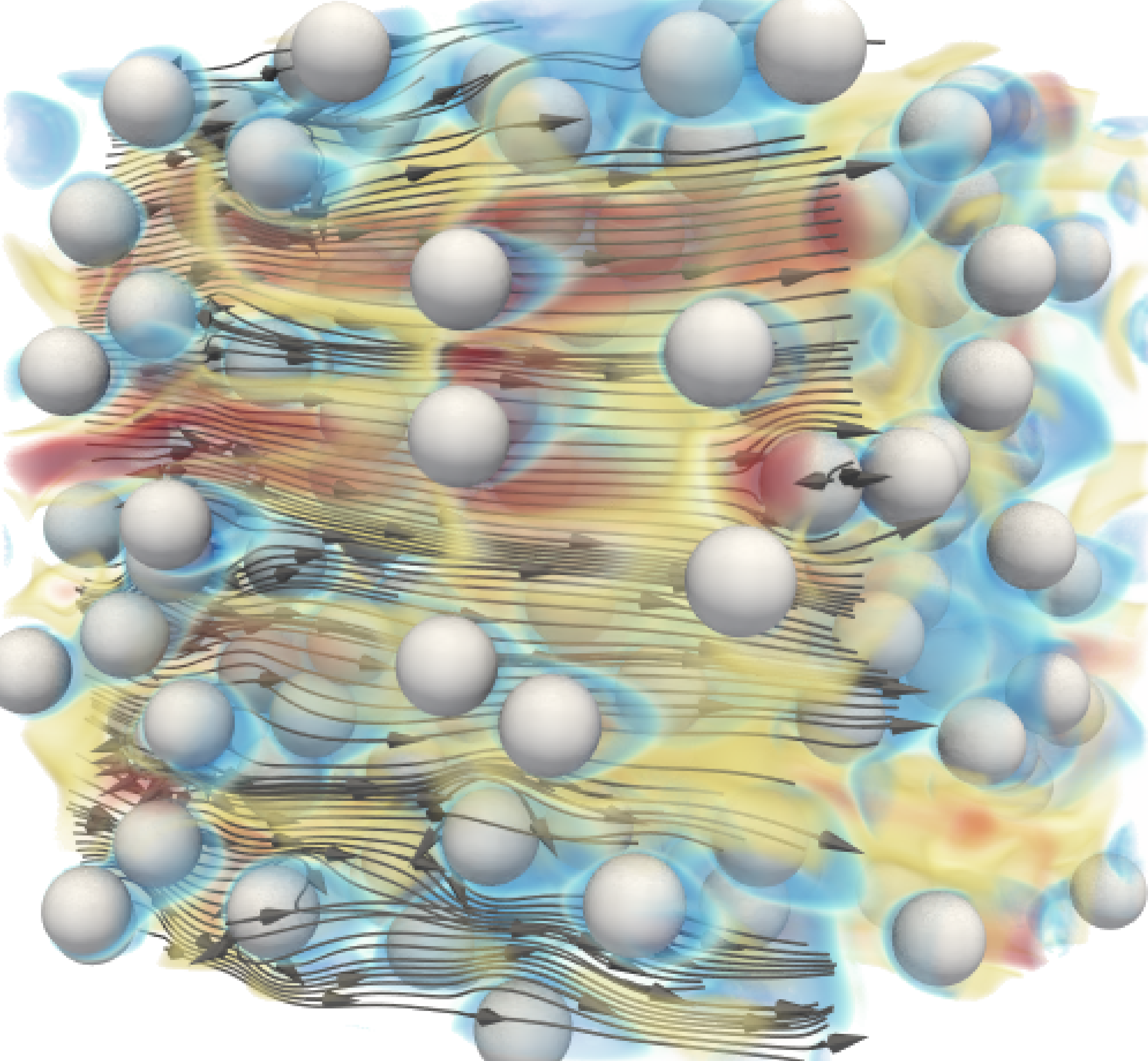
Figure 1: PR–DNS of homogeneous fluidization at ${\rm Re}_{m}=20$; $\rho_{p}/\rho_{f}=1000$; and $\langle\phi\rangle=0.1$. Arrows denote fluid streamlines, velocity magnitude shown in color.

Homogeneous fluidization of elastic smooth spheres provides a canonical flow that allows us to isolate key physics. A constant flow is exerted on the suspensions with mean Reynolds number, ${\rm Re}_{m}=(1-\left\langle\phi\right\rangle)\rho_{f}d_{p}\left|\left\langle\bm{w}\right\rangle\right|/\mu_{f}$, which drives the particles to a steady granular temperature (see Fig. 1). Here, $\langle\phi\rangle$ is the mean solids volume fraction, $\rho_{f}$ is the fluid density, $d_{p}$ is the particle diameter, $\left\langle\bm{w}\right\rangle=\left\langle\bm{u}_{f}\right\rangle-\left\langle\bm{v}_{p}\right\rangle$ is the mean slip velocity between the fluid $\left\langle\bm{u}_{f}\right\rangle$ and particles $\left\langle\bm{v}_{p}\right\rangle$, $\mu_{f}$ is the fluid dynamic viscosity, and $\left\langle\cdot\right\rangle$ denotes an ensemble average. The evolution of granular temperature in this system, $T=\left\langle\bm{v}_{p}^{\prime}\cdot\bm{v}_{p}^{\prime}\right\rangle/3$, is dictated by the covariance of fluctuating hydrodynamic acceleration $\bm{a}_{h}^{\prime}$ and particle velocity $\bm{v}_{p}^{\prime}$, which contains sources $S$ and sinks $\Gamma$ [12]

$$\frac{{\rm d}T}{{\rm d}t}=\frac{2}{3}\langle\bm{a}_{h}^{\prime}\cdot\bm{v}_{p}^{\prime}\rangle=S-\Gamma,$$ (1)

where the prime notation denotes a fluctuation from the ensemble average. Therefore, accurate descriptions for $\bm{a}_{h}^{\prime}$ are crucial to capturing $T(t)$.

For a particle subjected to hydrodynamic forces, its total translational velocity, $\bm{v}_{p}=\left\langle\bm{v}_{p}\right\rangle+\bm{v}_{p}^{\prime}$, follows

$$\frac{{\rm d}\bm{v}_{p}}{{\rm d}t}=\frac{1}{m_{p}}\int_{\partial\Omega}\bm{\tau}\bm{\cdot}\bm{n}\,{\rm d}S,$$ (2)

where $m_{p}$ is the particle mass and surface integration of the fluid stress tensor $\bm{\tau}$ (comprised of pressure and viscous stress) gives the total hydrodynamic acceleration $\bm{a}_{h}$. A model for $\bm{a}_{h}(t)$ has been obtained in the limit of an isolated sphere and Stokes flow by Basset [13], Boussinesq [14], and Oseen [15] that involves a superposition of forces from the undisturbed fluid flow, quasi-steady drag, added mass, and Basset history (the so-called BBO equations). Maxey and Riley [16] later extended this to non-uniform Stokes flow. At finite solids volume fractions and Reynolds numbers, analytical evaluation of the fluid stress integral is not tractable. Alternatively, correlations are often obtained from PR–DNS by ensemble averaging the net hydrodynamic force acting on a suspension. However, as shown in Fig. 1, particles interact with fluid wakes generated by their neighbors, leading to a distribution of hydrodynamic forces [17] that drive relative motion between particles. The application of a drag correlation, obtained from ensemble averaging, cannot reproduce the hydrodynamic force distributions obtained from PR–DNS. To properly account for said distribution, we apply the correlation of Tenneti et al. [18] to the instantaneous particle velocity and include a stochastic fluctuation $\bm{a}_{h}^{\prime\prime}$

$$\frac{1}{m_{p}}\int_{\partial\Omega}\bm{\tau}\bm{\cdot}\bm{n}\,{\rm d}S =\frac{1}{\tau_{d}}\left(\left\langle\bm{u}_{f}\right\rangle-\bm{v}_{p}\right)+\bm{a}_{h}^{\prime\prime}$$ (3)

where $1/\tau_{d}=F\left(\langle\phi\rangle,{\rm Re}_{m}\right)\left(1-\langle\phi\rangle\right)/\tau_{p}$ is the hydrodynamic time scale, and $\tau_{p}=\rho_{p}d_{p}^{2}/(18\mu_{f})$ is the Stokes time scale. Applying $\langle\cdot\rangle$ to Eq. (3) gives $\left\langle\bm{a}_{h}\right\rangle$. Removal of $\left\langle\bm{a}_{h}\right\rangle$ yields a reference frame that moves with the mean particle velocity and $\bm{a}_{h}^{\prime}=-\bm{v}_{p}^{\prime}/\tau_{d}+\bm{a}_{h}^{\prime\prime}$.

At the conditions considered here, hydrodynamic disturbances are attributed to pseudo-turbulent kinetic energy generated by the fluid boundary layers of neighboring particles [19, 20]. As a result, we describe $\bm{a}_{h}^{\prime\prime}$ with an appropriate acceleration Langevin equation [21]

$$\mathrm{d}\bm{v}_{p}^{\prime} =-\frac{1}{\tau_{d}}\bm{v}_{p}^{\prime}\,\mathrm{d}t+\bm{a}_{h}^{\prime\prime}\,\mathrm{d}t,$$ (4a)

$$\mathrm{d}\bm{a}_{h}^{\prime\prime} =-\frac{1}{\tau_{a^{\prime\prime}}}\bm{a}_{h}^{\prime\prime}\,\mathrm{d}t+\sqrt{\frac{2}{\tau_{a^{\prime\prime}}}}\sigma_{a^{\prime\prime}}\,\mathrm{d}\bm{W}_{t},$$ (4b)

where $\tau_{a^{\prime\prime}}$ is the integral time scale of the stochastic acceleration, $\sigma_{a^{\prime\prime}}$ is the standard deviation, and $\mathrm{d}\bm{W}_{t}$ is a Wiener process increment.

To quantify $S$ and $\Gamma$, one must evaluate the quadrant-conditioned acceleration-velocity covariance. Sources occur when the fluctuating acceleration is aligned with the fluctuating particle velocity (quadrants 1 and 3 in $a^{\prime}-v^{\prime}$ phase space). Analogously, sinks occur for the converse case (quadrants 2 and 4). Thus, we seek the probability distribution resulting from Eqs. (4a)–(4b). For constant coefficients, we derive the acceleration-velocity distribution in supplementary material § 1. Here, we report the salient result that $P\left(v^{\prime},a^{\prime};t\right)=\mathcal{N}\left(\bar{\bm{\Sigma}}^{-1}\right)$ is a joint normal with

$$\bar{\bm{\Sigma}}=\left[\begin{array}[]{cc}\frac{1}{\tau_{d}^{2}}\sigma_{v^{\prime}}^{2}(t)-\frac{1}{\tau_{d}}\sigma_{v^{\prime}a^{\prime\prime}}(t)+\sigma_{a^{\prime\prime}}^{2}&-\frac{1}{\tau_{d}}\sigma_{v^{\prime}}^{2}(t)+\sigma_{v^{\prime}a^{\prime\prime}}(t)\\ -\frac{1}{\tau_{d}}\sigma_{v^{\prime}}^{2}(t)+\sigma_{v^{\prime}a^{\prime\prime}}(t)&\sigma_{v^{\prime}}^{2}(t)\end{array}\right],$$ (7)

$$\sigma_{v^{\prime}}^{2}(t)=\sigma_{a^{\prime\prime}}^{2}\hat{\tau}^{+}\left[\tau_{d}\mathbb{E}_{2}+2\hat{\tau}^{-}\left(\mathbb{E}_{2}-\mathbb{E}_{3}\right)+\mathbb{C}_{0}\tau_{d}\left(1-\mathbb{E}_{2}\right)-2\rho_{0}\sqrt{\frac{\mathbb{C}_{0}\tau_{d}}{\hat{\tau}^{+}}}\hat{\tau}^{-}\left(\mathbb{E}_{2}-\mathbb{E}_{3}\right)\right],$$

$$\sigma_{v^{\prime}a^{\prime\prime}}(t)=\sigma_{a^{\prime\prime}}^{2}\hat{\tau}^{+}\left[\mathbb{E}_{3}+\rho_{0}\sqrt{\frac{\mathbb{C}_{0}\tau_{d}}{\hat{\tau}^{+}}}\left(1-\mathbb{E}_{3}\right)\right],\quad\mathbb{E}_{2}=\left\{1-\exp\left(-\frac{2t}{\tau_{d}}\right)\right\},\quad\mathbb{E}_{3}=\left\{1-\exp\left(-\frac{t}{\hat{\tau}^{+}}\right)\right\},$$

where $\hat{\tau}^{+}=\tau_{d}\tau_{a^{\prime\prime}}/(\tau_{d}+\tau_{a^{\prime\prime}})$, $\hat{\tau}^{-}=\tau_{d}\tau_{a^{\prime\prime}}/(\tau_{d}-\tau_{a^{\prime\prime}})$, $\rho_{0}=\sigma_{v^{\prime}a^{\prime\prime}}/(\sigma_{v^{\prime}}\,\sigma_{a^{\prime\prime}})$ is the initial correlation coefficient between the fluctuating velocity and stochastic acceleration, and $\mathbb{C}_{0}\geq 0$ is a proportionality constant that specifies the initial velocity variance $\sigma_{v^{\prime},0}^{2}$ as a fraction of the steady velocity variance $\sigma_{v^{\prime},\infty}^{2}=\sigma_{a^{\prime\prime}}^{2}\hat{\tau}^{+}\tau_{d}$. Following [22], we derive relations for the quadrant-covariance of a joint-normal (see supplementary material § 2)

$$S(t)=\frac{2\sqrt{\Sigma_{11}\Sigma_{22}}}{\pi}\left(\rho\arcsin{\rho}+\sqrt{1-\rho^{2}}+\frac{\pi}{2}\rho\right),$$ (8a)

$$\Gamma(t)=\frac{2\sqrt{\Sigma_{11}\Sigma_{22}}}{\pi}\left(\rho\arcsin{\rho}+\sqrt{1-\rho^{2}}-\frac{\pi}{2}\rho\right),$$ (8b)

where $\rho(t)=\Sigma_{12}/\sqrt{\Sigma_{11}\Sigma_{22}}$ is the correlation coefficient evaluated at time $t$.

Evaluation of Eq. (8) requires closure for the stochastic process. The acceleration time scale $\tau_{a^{\prime\prime}}$ is approximated with the mean-free time between successive collisions [23]

$$\tau_{a^{\prime\prime}}\approx\tau_{\rm col}=\frac{d_{p}}{24\langle\phi\rangle g_{0}}\sqrt{\frac{\pi}{T}},$$ (9)

where $g_{0}$ is the radial distribution function at contact [24]. The standard deviation $\sigma_{a^{\prime\prime}}$ is closed with a correlation obtained from PR–DNS of static particle assemblies

$$\sigma_{a^{\prime\prime}} =\sqrt{\frac{5}{9}}f_{\phi}^{\sigma_{F}}f_{\rm iso}\frac{(1-\langle\phi\rangle)\left|\langle\bm{w}\rangle\right|}{\tau_{p}},$$ (10a)

$$f_{\phi}^{\sigma_{F}} =6.52\langle\phi\rangle-22.56\langle\phi\rangle^{2}+49.90\langle\phi\rangle^{3},$$ (10b)

$$f_{\rm iso} =\left(1+0.15{\rm Re}_{m}^{0.687}\right).$$ (10c)

Here, $f_{\rm iso}$ represents the drag correction for an isolated particle using the classical correlation of Schiller and Naumann [25]. We note that the $5/9$ factor in Eq. (10a) is employed in the collisionless theory here to account for force anisotropy. Namely, the force variance extracted from PR–DNS is observed to be $\sim 3\times$ larger in the streamwise direction than the transverse directions. To account for the variable memory time scale $\tau_{a^{\prime\prime}}=f\left(T(t)\right)$, Eq. (7) is integrated forward in time by applying the solution to a time step $\Delta t$.

Analytical results are compared with PR–DNS benchmark data for two canonical flows at ${\rm Re}_{m}=20$; $\rho_{p}/\rho_{f}=1000$; $\langle\phi\rangle=0.1$. Namely, homogeneous heating (HHS) and homogeneous cooling (HCS) systems are examined in detail. In the former system, particles are initialized as $T_{0}=0$, while the latter is initialized as $T_{0}>T_{\infty}$, with $T_{\infty}$ the steady granular temperature. Considering the dimensionless source $\hat{S}(t)=S(t)\tau_{p}/\left((1-\langle\phi\rangle)^{2}\left|\left\langle\bm{w}\right\rangle\right|^{2}\right)$, and analogous dimensionless sink $\hat{\Gamma}(t)$, we observe strong agreement between analytical predictions and PR–DNS data (see Figs. 2–3).

A direct consequence of accurately characterizing $S(t)$ and $\Gamma(t)$ is that the theory captures the temporal evolution of ${\rm Re}_{T}=\rho_{f}d_{p}\sqrt{T}/\mu_{f}$ (see Fig. 4). The ability of Eq. (7) to capture the granular temperature dynamics speaks to the statistical equivalence between the acceleration Langevin model and homogeneous fluidization of elastic particles at finite Reynolds numbers. To demonstrate equivalence in a more quantitative manner we compare the acceleration-velocity probability distribution to scatter plots obtained from PR–DNS (see Fig. 5). Again, data extracted from PR–DNS is well characterized by $P\left(v^{\prime},a^{\prime};t\right)$ obtained from integration of Eq. (7). In the HHS (top panels of Fig. 5), granular temperature is dominated by hydrodynamic sources (quadrants 1 and 3) at early time that become balanced by the sinks, leading to a sustained particle velocity variance. By contrast, hydrodynamic sinks (quadrants 2 and 4) are dominant in the HCS (bottom panels of Fig. 5) since the system is initialized with an over-prescribed velocity variance.

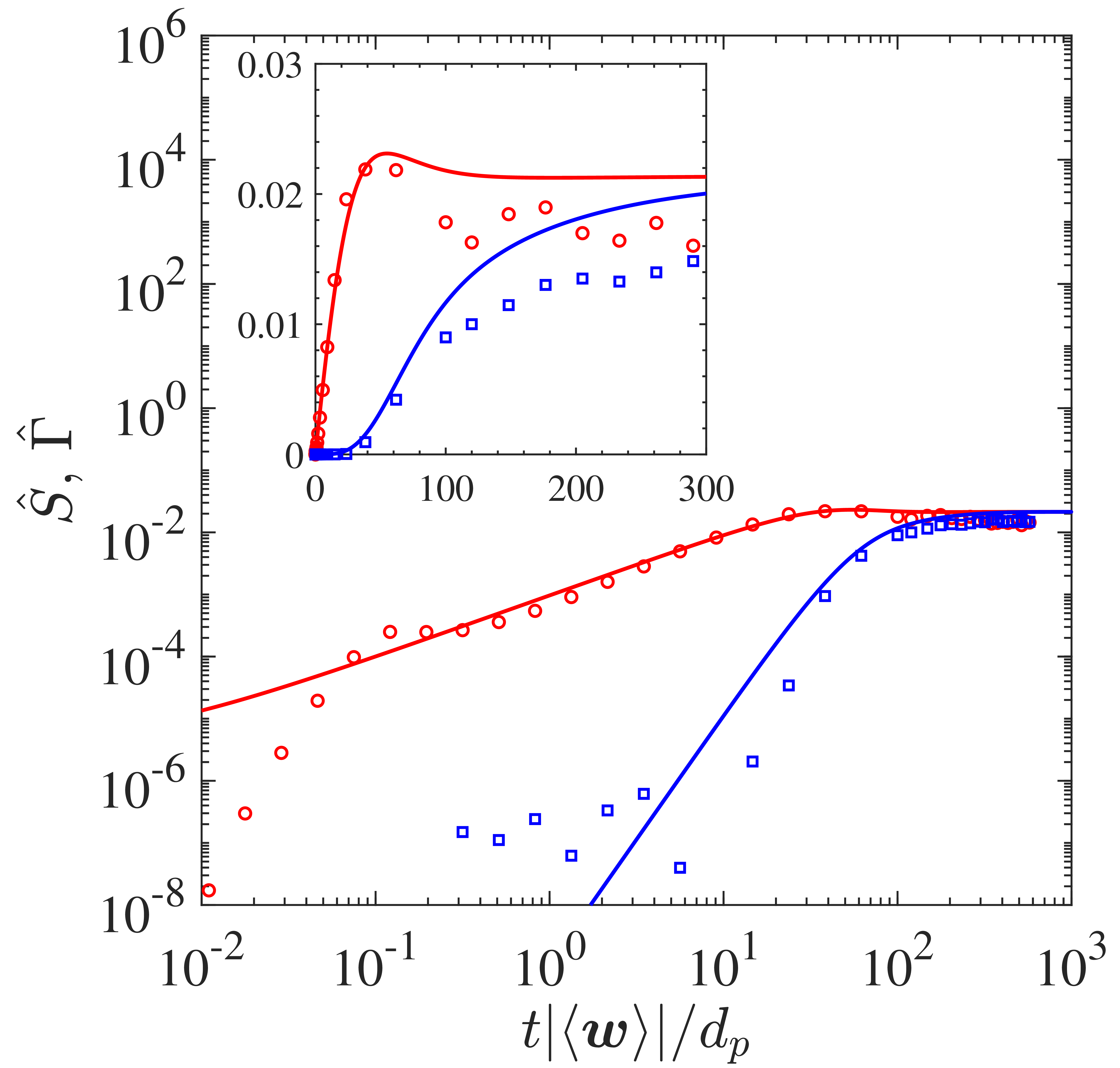
Figure 2: Non-dimensional source (red) and sink (blue) in the HHS. Analytic solution obtained from Eq. (8) with $\rho_{0}=1$ (lines), PR–DNS data (symbols). The inset shows the same data with linear scaling.

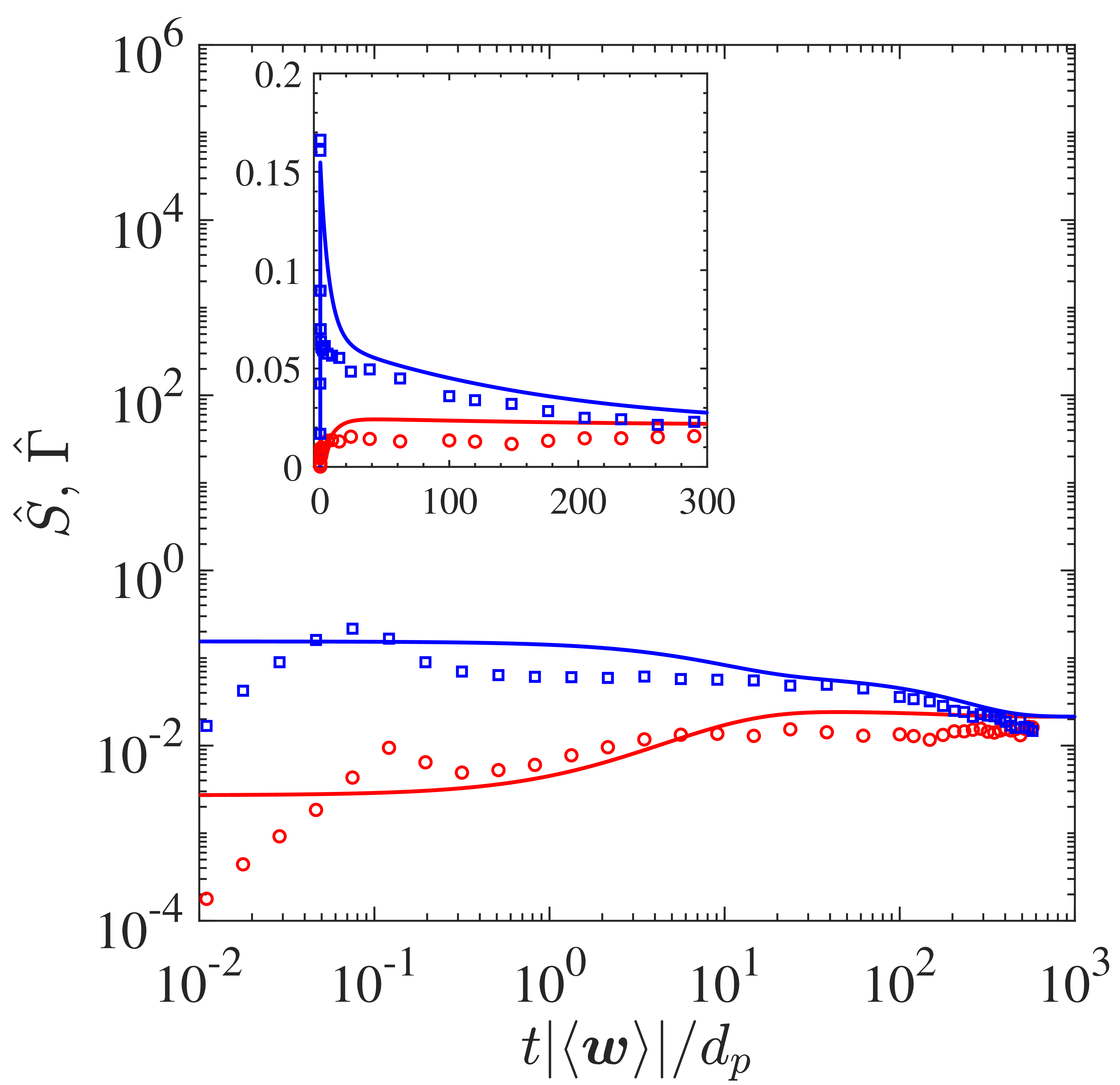
Figure 3: Same legend as Fig. 2 for the HCS but with $\rho_{0}=-0.75$.

While the present theory is designed around inertial particles at high density ratios $\rho_{p}/\rho_{f}\gg 1$, it is beneficial to consider the behavior across density ratio. Previous PR–DNS studies concluded that $T_{\infty}\sim\rho_{f}/\rho_{p}$ for $\rho_{p}/\rho_{f}\geq 100$ [12, 26]. However, such scaling leads to unrealistic granular temperature for low density particles. Tavanashad et al. [27] showed that $T_{\infty}$ levels off at low density ratio due to the additional dissipation associated with unsteady hydrodynamic forces (e.g., added mass and Basset history). Taking $\lim_{t\to\infty}\sigma_{v^{\prime}}^{2}(t)$ yields an algebraic relation $T_{\infty}=\sigma_{a^{\prime\prime}}^{2}\tau_{d}^{2}\tau_{a^{\prime\prime}}(T_{\infty})/(\tau_{d}+\tau_{a^{\prime\prime}}(T_{\infty}))$.

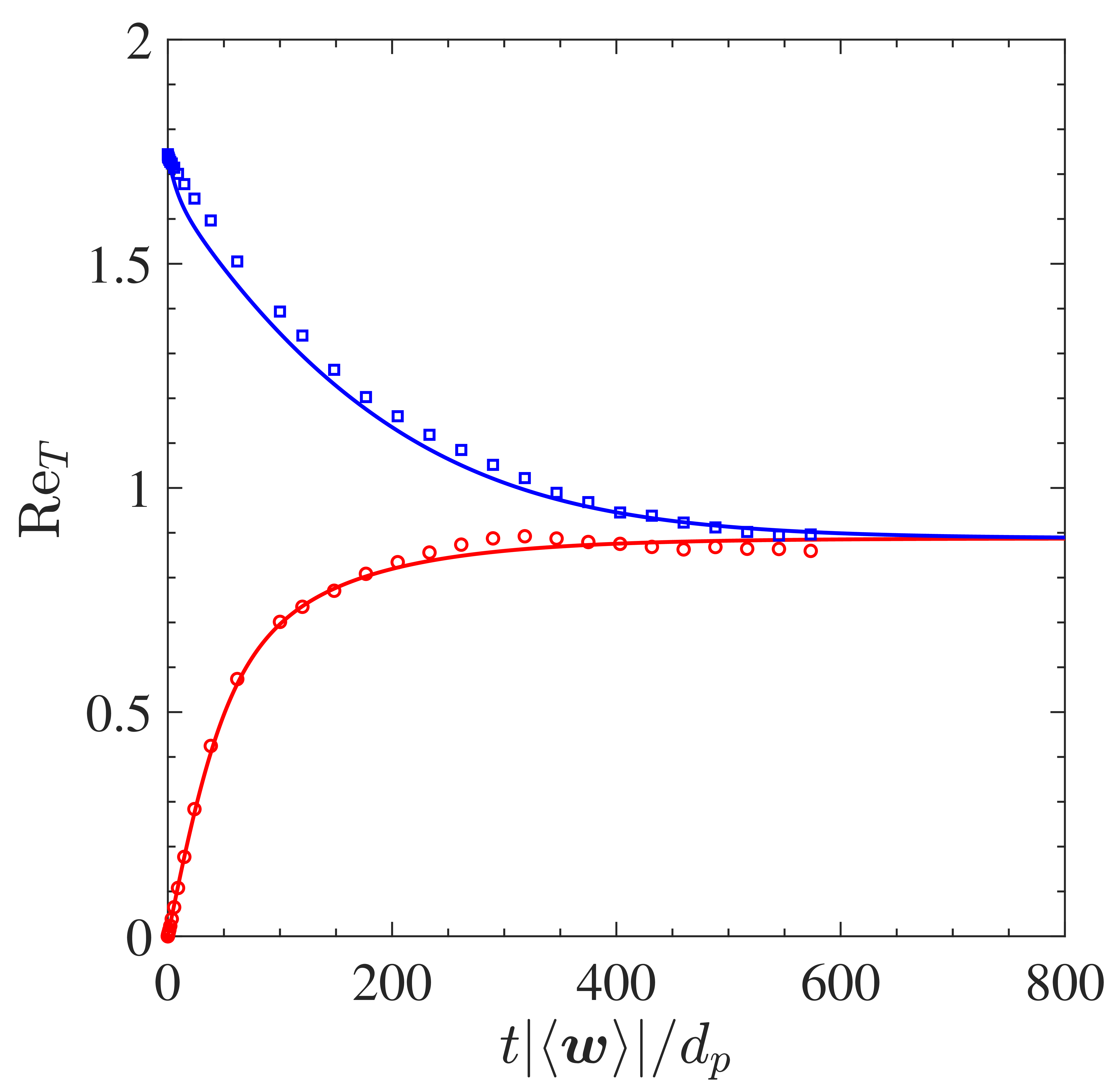
Figure 4: Evolution of non-dimensional granular temperature for the HHS (red) and HCS (blue). Analytic solution (lines), PR–DNS (symbols).

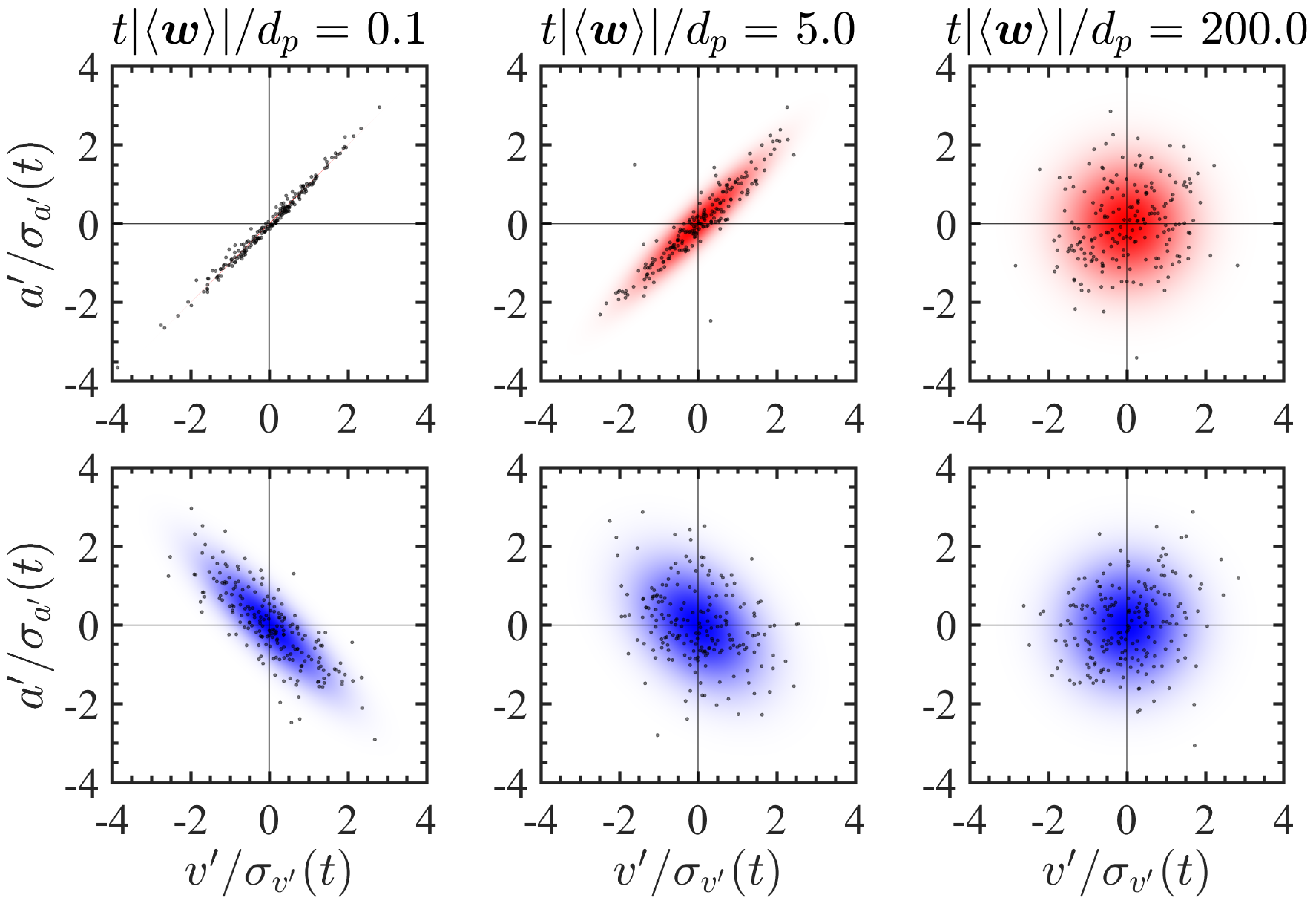
Figure 5: Joint PDFs of the fluctuating particle acceleration and fluctuating particle velocity for the HHS (top) and HCS (bottom). Analytic solution (color), PR–DNS (symbols). The first and third quadrant correspond to sources of granular temperature and the second and fourth quadrant correspond to dissipation.

We solve said relation to ascertain the behavior of the present theory across a wide range of density ratios (see Fig. 6). As opposed to earlier correlations obtained from PR–DNS of inertial particles [12, 26], the acceleration Langevin solution is capable of predicting the tail off of granular temperature reported by Tavanashad et al. [27]. The asymptotic behavior of the theory may be seen by noting that $\tau_{d}=f(\rho_{p})$ and $\tau_{d}\ll\tau_{a^{\prime\prime}}$ as $\rho_{p}/\rho_{f}\rightarrow 0$.

While results presented here at low density ratio are incipient, the modeling paradigm shows promise as a viable starting place for developing a theory across particle density ratio. In this spirit, $\sigma_{a^{\prime\prime}}$ correlations may be obtained beyond the static particle limit and utilized alongside drag correlations that are valid across density ratio [28]. These efforts may allow extension of the present theory beyond inertial particles — i.e., a general description for fluid-mediated sources to granular temperature that is valid from gas–solid to bubbly flows appears possible.

This work was supported by National Science Foundation under grants CBET-1904742 and CBET-1438143.

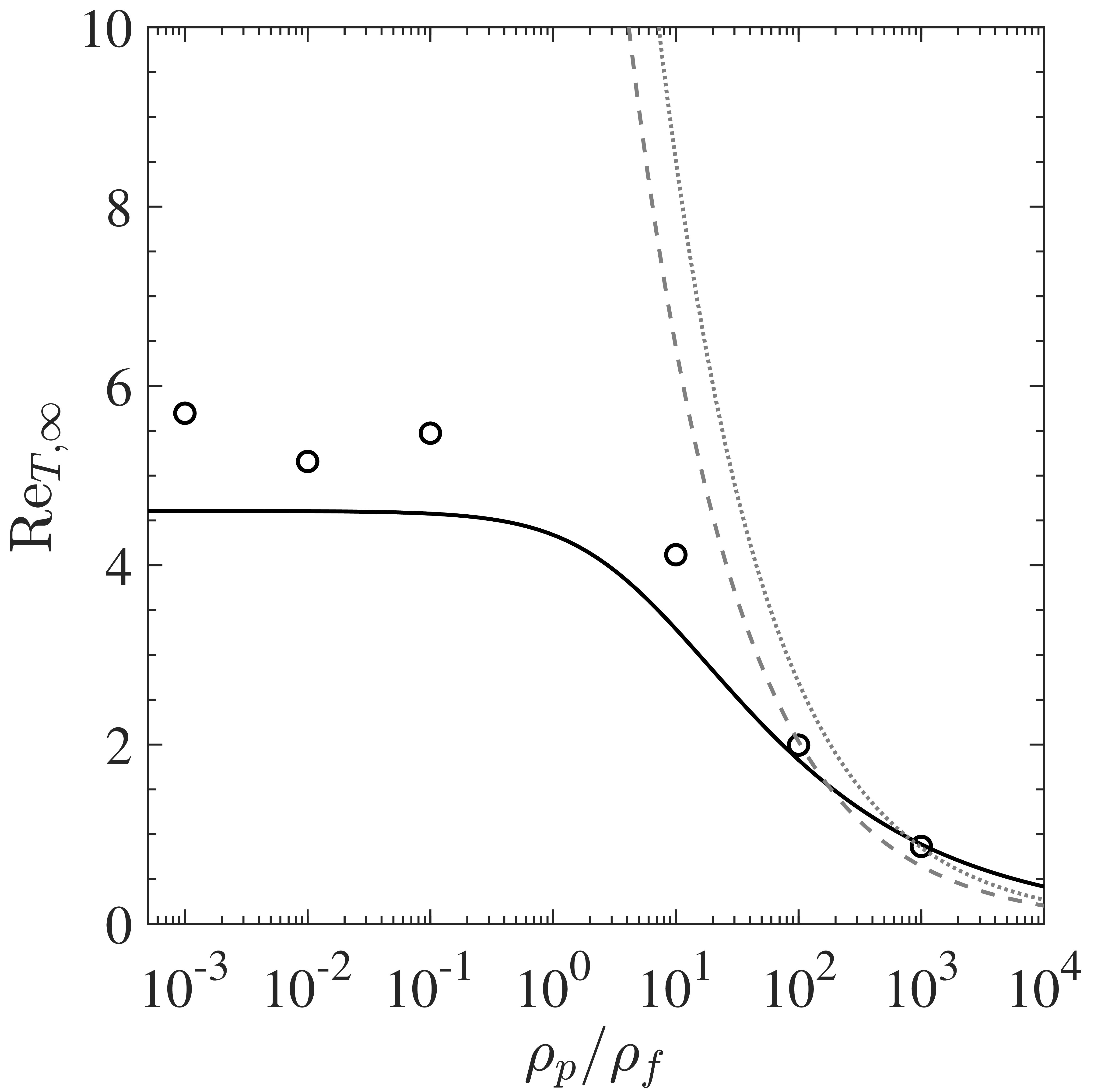
Figure 6: Non-dimensional granular temperature at steady state as a function of density ratio. Analytical solution (solid line), PR–DNS of Tavanashad et al. [27] (symbols), correlation of Tenneti et al. [12] (dashed line), correlation of Tang et al. [26] (dotted line).

Supplemental Material:
Fluid-mediated sources of granular temperature at finite Reynolds numbers

I The joint acceleration-velocity distribution

I.1 General formulation

Following our previous works on neighbor-induced drag disturbances [29, 21], we consider a stochastic approach for the hydrodynamic force perturbation induced by particles in close proximity. Specifically, the following stochastic differential equations (SDEs) are considered

$$\mathrm{d}\bm{x}_{p}^{\prime} =\bm{v}_{p}^{\prime}\,\mathrm{d}t,$$ (S1a)

$$\mathrm{d}\bm{v}_{p}^{\prime} =-\frac{1}{\tau_{d}}\bm{v}_{p}^{\prime}\,\mathrm{d}t+\bm{a}_{h}^{\prime\prime}\,\mathrm{d}t,$$ (S1b)

$$\mathrm{d}\bm{a}_{h}^{\prime\prime} =-\frac{1}{\tau_{a^{\prime\prime}}}\bm{a}_{h}^{\prime\prime}\,\mathrm{d}t+\sqrt{\frac{2}{\tau_{a^{\prime\prime}}}}\sigma_{a^{\prime\prime}}\,\mathrm{d}\bm{W}_{t},$$ (S1c)

where $\bm{x}_{p}^{\prime}$, $\bm{v}_{p}^{\prime}$, $\bm{a}_{h}^{\prime\prime}$ are the fluctuating position, velocity, and hydrodynamic acceleration, respectively, $\tau_{a^{\prime\prime}}$ is the fluctuating acceleration memory, $\sigma_{a^{\prime\prime}}=\sigma_{F^{\prime\prime}}/m_{p}$ is the fluctuating acceleration standard deviation, $\sigma_{F^{\prime\prime}}$ is the standard deviation in drag force, and $m_{p}$ is the particle mass. $\tau_{d}$ is the drag response time scale obtained from applying the correlation of Tenneti et al. [30] in the same manner as Appendix C of Lattanzi et al. [29]. When deriving the weak (distribution) solution to the set of stochastic differential equations, we consider the coefficients $(\tau_{d};\,\tau_{a^{\prime\prime}};\,\sigma_{a^{\prime\prime}})$ to be constant. Physical arguments are provided in § I.2 for why $\sigma_{a^{\prime\prime}}$ may be approximated as constant in the homogeneous system. However, the acceleration memory is approximated with the mean-free-time between collisions (Eq. 7 in main text) and will lead to $\tau_{a^{\prime\prime}}=f(T(t))$, where $T$ is the granular temperature (velocity variance). The constant coefficient solution obtained below (see Eq. (S18)) may be integrated forward in time to account for the functional dependence of $\tau_{a^{\prime\prime}}$. Supplementary code is provided to demonstrate how solutions derived herein yield the reported results. More specifically, we include a library of solutions (AL_Lib.m) that is utilized by integration routines for the homogeneous heating (AL_HHS_Example.m) and homogeneous cooling (AL_HCS_Example.m) cases to reproduce Figures 2–4 in the main text.

The Fokker-Planck equation resulting from Eqs. (S1a)–(S1c) is given by

$$\frac{\partial P}{\partial t}+\nabla_{\bm{x}^{\prime}}\cdot\left(\bm{v}^{\prime}P\right)+\nabla_{\bm{v}^{\prime}}\cdot\left[\left(\bm{a}^{\prime\prime}-\frac{1}{\tau_{d}}\bm{v}^{\prime}\right)P\right]-\frac{1}{\tau_{a^{\prime\prime}}}\nabla_{\bm{a}^{\prime\prime}}\cdot\left(\bm{a}^{\prime\prime}P\right)=\frac{\sigma_{a^{\prime\prime}}^{2}}{\tau_{a^{\prime\prime}}}\Delta_{\bm{a}^{\prime\prime}}P,$$ (S2)

where $P(\bm{x}^{\prime},\bm{v}^{\prime},\bm{a}^{\prime\prime};t|\bm{y}^{\prime},\bm{u}^{\prime},\bm{b}^{\prime\prime};s)$ is the probability density function and subscripts denote the phase space variables being differentiated. Considering Eq. (S2) in 1D, we integrate over $x^{\prime}$ to obtain the evolution of the joint acceleration-velocity distribution $P(v^{\prime},a^{\prime\prime};t|u^{\prime},b^{\prime\prime};s)$

$$\frac{\partial P}{\partial t}+\frac{\partial}{\partial v^{\prime}}\left[\left(a^{\prime\prime}-\frac{1}{\tau_{d}}v^{\prime}\right)P\right]-\frac{1}{\tau_{a^{\prime\prime}}}\frac{\partial}{\partial a^{\prime\prime}}\left(a^{\prime\prime}P\right)=\frac{\sigma_{a^{\prime\prime}}^{2}}{\tau_{a^{\prime\prime}}}\frac{\partial^{2}P}{{\partial a^{\prime\prime}}^{2}}.$$ (S3)

Applying Fourier transform to Eq. (S3), $\mathcal{F}\left[P(\bm{x};t)\right]=\mathcal{P}(\bm{k};t)$, we obtain

$$\frac{\partial\mathcal{P}}{\partial t}+\frac{k_{v^{\prime}}}{\tau_{d}}\frac{\partial\mathcal{P}}{\partial k_{v^{\prime}}}+\left[\frac{k_{a^{\prime\prime}}}{\tau_{a^{\prime\prime}}}-k_{v^{\prime}}\right]\frac{\partial\mathcal{P}}{\partial k_{a^{\prime\prime}}}=-\frac{k_{a^{\prime\prime}}^{2}\sigma_{a^{\prime\prime}}^{2}}{\tau_{a^{\prime\prime}}}\mathcal{P}.$$ (S4)

Employing method of characteristics (MOC), we seek a parameterizaton variable $s$

$$\frac{{\rm d}\mathcal{P}(t(s),k_{v^{\prime}}(s),k_{a^{\prime\prime}}(s))}{{\rm d}s}=\frac{\partial\mathcal{P}}{\partial t}\frac{{\rm d}t}{{\rm d}s}+\frac{\partial\mathcal{P}}{\partial k_{v^{\prime}}}\frac{{\rm d}k_{v^{\prime}}}{{\rm d}s}+\frac{\partial\mathcal{P}}{\partial k_{a^{\prime\prime}}}\frac{{\rm d}k_{a^{\prime\prime}}}{{\rm d}s},$$ (S5)

and match the coefficients of Eq. (S5) with Eq. (S4) to yield a system of equations

$$\frac{{\rm d}t}{{\rm d}s} =1$$ (S6a)

$$\frac{{\rm d}k_{v^{\prime}}}{{\rm d}s} =\frac{k_{v^{\prime}}}{\tau_{d}}$$ (S6b)

$$\frac{{\rm d}k_{a^{\prime\prime}}}{{\rm d}s} =\frac{k_{a^{\prime\prime}}}{\tau_{a^{\prime\prime}}}-k_{v^{\prime}}$$ (S6c)

$$\frac{{\rm d}\mathcal{P}}{{\rm d}s} =-\frac{k_{a^{\prime\prime}}^{2}\sigma_{a^{\prime\prime}}^{2}}{\tau_{a^{\prime\prime}}}\mathcal{P}.$$ (S6d)

Integrating the system of equations gives

$$t =s+C_{0},$$ (S7a)

$$k_{v^{\prime}} =C_{1}\exp\left(\frac{s}{\tau_{d}}\right),$$ (S7b)

$$k_{a^{\prime\prime}} =C_{1}\hat{\tau}^{-}\exp\left(\frac{s}{\tau_{d}}\right)+C_{2}\exp\left(\frac{s}{\tau_{a^{\prime\prime}}}\right),$$ (S7c)

$$\mathcal{P} =C_{3}\exp\left(-\frac{\sigma_{a^{\prime\prime}}^{2}}{2}\left[\left(C_{1}\hat{\tau}^{-}\right)^{2}\frac{\tau_{d}}{\tau_{a^{\prime\prime}}}\exp\left(\frac{2s}{\tau_{d}}\right)+C_{2}^{2}\exp\left(\frac{2s}{\tau_{a^{\prime\prime}}}\right)+4C_{1}C_{2}\frac{\hat{\tau}^{-}\hat{\tau}^{+}}{\tau_{a^{\prime\prime}}}\exp\left(\frac{s}{\hat{\tau}^{+}}\right)\right]\right),$$ (S7d)

where $\hat{\tau}^{-}=\tau_{d}\tau_{a^{\prime\prime}}/(\tau_{d}-\tau_{a^{\prime\prime}})$ and $\hat{\tau}^{+}=\tau_{d}\tau_{a^{\prime\prime}}/(\tau_{d}+\tau_{a^{\prime\prime}})$. Taking $C_{0}=0$, we show the MOC solution is invertible, viz.

$$s =t,$$ (S8a)

$$C_{1} =k_{v^{\prime}}\exp\left(-\frac{t}{\tau_{d}}\right),$$ (S8b)

$$C_{2} =\left[k_{a^{\prime\prime}}-k_{v^{\prime}}\hat{\tau}^{-}\right]\exp\left(-\frac{t}{\tau_{a^{\prime\prime}}}\right).$$ (S8c)

To obtain a closed-form solution one must impose an initial condition $\mathcal{P}(0)$, invert constants via Eqs. (S8a)–(S8c), and apply an inverse Fourier transform $\mathcal{F}^{-1}\left[\mathcal{P}(\bm{k};t)\right]=P(\bm{x};t)$. We consider a general initial condition in the following subsection.

I.2 Arbitrarily correlated initial condition

We consider particles with specified initial velocity variance $\sigma_{v^{\prime},0}^{2}$ and initial acceleration-velocity covariance $\sigma_{v^{\prime}a^{\prime\prime},0}=\rho_{0}\sigma_{a^{\prime\prime}}\sigma_{v^{\prime},0}$. The initial condition allows us to consider general fluidization, which will encompasses the cooling and heating systems probed by PR–DNS studies [18, 12, 27]. For inertial particles, fluid boundary layers will develop on much smaller time scales than the particle velocity variance; thus, we consider the fluctuating hydrodynamic acceleration to be fully-developed (steady solution to Ornstein-Uhlenbeck process in Eq. (S1c)). The correlated initial condition yields

$$\mathcal{F}\left[\mathcal{N}\left(\bar{\bm{\Sigma}}^{-1}\right)\right]=\exp\left(-\frac{k_{a^{\prime\prime}}^{2}\sigma_{a^{\prime\prime}}^{2}}{2}-\frac{k_{v^{\prime}}^{2}\sigma_{v^{\prime},0}^{2}}{2}-k_{a^{\prime\prime}}k_{v^{\prime}}\sigma_{v^{\prime}a^{\prime\prime},0}\right),$$ (S9)

where $\mathcal{N}\left(\bar{\bm{\Sigma}}^{-1}\right)$ is the normal distribution with covariance matrix $\bar{\bm{\Sigma}}$. Evaluating Eq. (S9) at $k_{i}(0)$ gives the initial condition

$$\mathcal{P}(0)=\exp\left(-\frac{\sigma_{a^{\prime\prime}}^{2}}{2}\left[\left(C_{1}\hat{\tau}^{-}\right)^{2}+C_{2}^{2}+2C_{1}C_{2}\hat{\tau}^{-}\right]-\frac{\sigma_{v^{\prime},0}^{2}}{2}C_{1}^{2}-\sigma_{v^{\prime}a^{\prime\prime},0}\left[C_{1}^{2}\hat{\tau}^{-}+C_{1}C_{2}\right]\right),$$ (S10)

which allows the $C_{3}$ constant to be obtained

$$C_{3}= \exp\left(\frac{\sigma_{a^{\prime\prime}}^{2}}{2}\left[\left(C_{1}\hat{\tau}^{-}\right)^{2}\left(\frac{\tau_{d}}{\tau_{a^{\prime\prime}}}-1\right)+4C_{1}C_{2}\frac{\hat{\tau}^{-}\hat{\tau}^{+}}{\tau_{a^{\prime\prime}}}-2C_{1}C_{2}\hat{\tau}^{-}\right]\right)\times$$ (S11)

$$\exp\left(-\frac{\sigma_{v^{\prime},0}^{2}}{2}C_{1}^{2}-\sigma_{v^{\prime}a^{\prime\prime},0}\left[C_{1}^{2}\hat{\tau}^{-}+C_{1}C_{2}\right]\right).$$

After inverting the constants ($C_{1}$; $C_{2}$), and a considerable amount of algebra, the joint distribution solution in wave-space is obtained

$$\mathcal{P}(k_{v^{\prime}},k_{a^{\prime\prime}};t)=\exp\left(-\frac{k_{a^{\prime\prime}}^{2}}{2}\sigma_{a^{\prime\prime}}^{2}-\frac{k_{v^{\prime}}^{2}}{2}\sigma_{v^{\prime}}^{2}(t)-k_{a^{\prime\prime}}k_{v^{\prime}}\sigma_{v^{\prime}a^{\prime\prime}}(t)\right),$$ (S12a)

$$\sigma_{v^{\prime}}^{2}(t)=\sigma_{a^{\prime\prime}}^{2}\hat{\tau}^{+}\left[\tau_{d}\mathbb{E}_{2}+2\hat{\tau}^{-}\left(\mathbb{E}_{2}-\mathbb{E}_{3}\right)+\mathbb{C}_{0}\tau_{d}\left(1-\mathbb{E}_{2}\right)-2\rho_{0}\sqrt{\frac{\mathbb{C}_{0}\tau_{d}}{\hat{\tau}^{+}}}\hat{\tau}^{-}\left(\mathbb{E}_{2}-\mathbb{E}_{3}\right)\right],$$ (S12b)

$$\sigma_{v^{\prime}a^{\prime\prime}}(t)=\sigma_{a^{\prime\prime}}^{2}\hat{\tau}^{+}\left[\mathbb{E}_{3}+\rho_{0}\sqrt{\frac{\mathbb{C}_{0}\tau_{d}}{\hat{\tau}^{+}}}\left(1-\mathbb{E}_{3}\right)\right],$$ (S12c)

$$\mathbb{E}_{2}=\left\{1-\exp\left(-\frac{2t}{\tau_{d}}\right)\right\},$$ (S12d)

$$\mathbb{E}_{3}=\left\{1-\exp\left(-\frac{t}{\hat{\tau}^{+}}\right)\right\}.$$ (S12e)

$\mathbb{C}_{0}\geq 0$ is a proportionality constant that specifies the initial velocity variance $\sigma_{v^{\prime},0}^{2}$ as a fraction of the steady velocity variance $\sigma_{v^{\prime},\infty}^{2}=\sigma_{a^{\prime\prime}}^{2}\hat{\tau}^{+}\tau_{d}$. Similarly, $\rho_{0}\in\left[-1\,1\right]$ is the initial correlation coefficient that specifies the initial covariance $\sigma_{v^{\prime}a^{\prime\prime},0}$. Since Eq. (S12a) is joint-normal in wave-space, it will also be joint-normal in physical space. Furthermore, taking $\lim\mathbb{C}_{0}\rightarrow 0$ and $\lim\rho_{0}\rightarrow 0$ shows that the velocity variance $\sigma_{v^{\prime}}^{2}(t)$ and acceleration-velocity covariance $\sigma_{v^{\prime}a^{\prime\prime}}(t)$ match the solutions provided in [29].

I.3 Total acceleration distribution

The total fluctuating hydrodynamic acceleration $\bm{a}_{h}^{\prime}$, right hand side of Eq. (S1b), includes contributions from deterministic drag and stochastic fluctuations

$$\bm{a}_{h}^{\prime}=-\frac{1}{\tau_{d}}\bm{v}_{p}^{\prime}+\bm{a}_{h}^{\prime\prime}.$$ (S13)

To compare with PR–DNS, we require $P(\bm{v}^{\prime},\bm{a}^{\prime};t)$ rather than $P(\bm{v}^{\prime},\bm{a}^{\prime\prime};t)$. Thus, we seek to characterize the variances and covariances of total fluctuating hydrodynamic acceleration. The covariance tensors are given by

$$\left\langle\bm{a}_{h}^{\prime}\otimes\bm{a}_{h}^{\prime}\right\rangle =\frac{1}{\tau_{d}^{2}}\left\langle\bm{v}_{p}^{\prime}\otimes\bm{v}_{p}^{\prime}\right\rangle-\frac{1}{\tau_{d}}\left\langle\bm{v}_{p}^{\prime}\otimes\bm{a}_{h}^{\prime\prime}\right\rangle+\left\langle\bm{a}_{h}^{\prime\prime}\otimes\bm{a}_{h}^{\prime\prime}\right\rangle,$$ (S14a)

$$\left\langle\bm{v}_{p}^{\prime}\otimes\bm{a}_{h}^{\prime}\right\rangle =-\frac{1}{\tau_{d}}\left\langle\bm{v}_{p}^{\prime}\otimes\bm{v}_{p}^{\prime}\right\rangle+\left\langle\bm{v}_{p}^{\prime}\otimes\bm{a}_{h}^{\prime\prime}\right\rangle.$$ (S14b)

Substituting results from Eqs. (S12b)–(S12c), we then obtain

$$\sigma_{a^{\prime}}^{2} =\frac{1}{\tau_{d}^{2}}\sigma_{v^{\prime}}^{2}-\frac{1}{\tau_{d}}\sigma_{v^{\prime}a^{\prime\prime}}+\sigma_{a^{\prime\prime}}^{2},$$ (S15a)

$$\sigma_{v^{\prime}a^{\prime}} =-\frac{1}{\tau_{d}}\sigma_{v^{\prime}}^{2}+\sigma_{v^{\prime}a^{\prime\prime}}.$$ (S15b)

Therefore, the fluctuating acceleration-velocity distribution $P(\bm{v}^{\prime},\bm{a}^{\prime};t)$ is a normal distribution $\mathcal{N}\left(\bar{\bm{\Sigma}}^{-1}\right)$ with time dependent covariance tensor given by

$$\bar{\bm{\Sigma}} =\left[\begin{array}[]{cc}\sigma_{a^{\prime}}^{2}(t)&\sigma_{v^{\prime}a^{\prime}}(t)\\ \sigma_{v^{\prime}a^{\prime}}(t)&\sigma_{v^{\prime}}^{2}(t)\end{array}\right].$$ (S18)

II Evolution of sources & sinks

II.1 Quadrant-covariance integrals

As described in Tenneti et al. [12], the fluctuating acceleration-velocity covariance dictates the temporal evolution of granular temperature in homogeneous fluidization of elastic particles. For a given particle, the sign of the covariance dictates if the acceleration acts as a source (positive; $a^{\prime}-v^{\prime}$ quadrants 1 & 3) or a sink (negative; $a^{\prime}-v^{\prime}$ quadrants 2 & 4). Therefore, to quantify the sources and sinks produced by the acceleration Langevin model, the quadrant-conditioned covariances must be computed

$$2\left\langle v^{\prime}a^{\prime}\right\rangle \equiv S-\Gamma=4\int_{0}^{\infty}\int_{0}^{\infty}v^{\prime}a^{\prime}\,\mathcal{N}\left(\bar{\bm{\Sigma}}^{-1}\right)\,{\rm d}a^{\prime}\,{\rm d}v^{\prime}-4\int_{-\infty}^{0}\int_{0}^{\infty}v^{\prime}a^{\prime}\,\mathcal{N}\left(\bar{\bm{\Sigma}}^{-1}\right)\,{\rm d}a^{\prime}\,{\rm d}v^{\prime},$$ (S19)

where $\mathcal{N}\left(\bar{\bm{\Sigma}}^{-1}\right)$ is the derived normal probability distribution with covariance matrix given in Eq. (S18), $S$ denotes the source, and $\Gamma$ denotes the sink. To evaluate the integrals given in Eq. (S19), we proceed similar to the derivation provided in Stuart and Ord [22]. For the source integral, substituting the Fourier transform of the characteristic function in place of the normal distribution function yields

$$S=\frac{4}{(2\pi)^{2}}\int_{0}^{\infty}\int_{0}^{\infty}x_{1}x_{2}\int_{-\infty}^{\infty}\int_{-\infty}^{\infty}\exp\left(-i\bm{k}^{\intercal}\bm{x}-\frac{1}{2}\bm{k}^{\intercal}\bar{\bm{\Sigma}}\bm{k}\right){\rm d}\bm{k}\,{\rm d}\bm{x},$$ (S20)

where $\bm{x}=\left[v^{\prime}\,a^{\prime}\right]^{\intercal}$ and $\bm{k}=[k_{v^{\prime}}\,k_{a^{\prime}}]^{\intercal}$. Exchanging the order of integration and employing the identity

$$x_{j}\exp\left(-ik_{j}x_{j}\right)=i\frac{\partial}{\partial k_{j}}\left(\exp\left(-ik_{j}x_{j}\right)\right),$$ (S21)

where no summation over $j$ is implied, leads to

$$S=\frac{1}{\pi^{2}}\int_{-\infty}^{\infty}\int_{-\infty}^{\infty}\exp\left(-\frac{1}{2}\bm{k}^{\intercal}\bar{\bm{\Sigma}}\bm{k}\right)\prod_{j=1}^{2}\left(i\frac{\partial}{\partial k_{j}}\right)\int_{0}^{\infty}\int_{0}^{\infty}\exp\left(-i\bm{k}^{\intercal}\bm{x}\right){\rm d}\bm{x}\,{\rm d}\bm{k}.$$ (S22)

The inner most integrals over $\bm{x}$ may be interpreted as the Fourier transforms of the Heaviside function, which have principal values $\prod_{j}\left(ik_{j}\right)^{-1}$. After evaluating the derivatives, one obtains

$$S=\frac{1}{\pi^{2}}\int_{-\infty}^{\infty}\int_{-\infty}^{\infty}\exp\left(-\frac{1}{2}\bm{k}^{\intercal}\bar{\bm{\Sigma}}\bm{k}\right)\frac{1}{k_{v^{\prime}}^{2}k_{a^{\prime}}^{2}}{\rm d}\bm{k}.$$ (S23)

The exponential in Eq. (S23) will contain a covariance term $-\rho\sigma_{v^{\prime}}\sigma_{a^{\prime}}k_{v^{\prime}}k_{a^{\prime}}$, where $\rho$ is the correlation coefficient. Differentiating both sides twice with respect to $\rho$ yields

$$\frac{{\rm d}^{2}S}{{\rm d}\rho^{2}}=\frac{\sigma_{v^{\prime}}^{2}\sigma_{a^{\prime}}^{2}}{\pi^{2}}\int_{-\infty}^{\infty}\int_{-\infty}^{\infty}\exp\left(-\frac{1}{2}\bm{k}^{\intercal}\bar{\bm{\Sigma}}\bm{k}\right){\rm d}\bm{k}.$$ (S24)

The above integral will yield the reciprocal of the normalization constant for a bi-normal distribution

$$\frac{{\rm d}^{2}S}{{\rm d}\rho^{2}}\equiv\frac{\sigma_{v^{\prime}}^{2}\sigma_{a^{\prime}}^{2}}{\pi^{2}}2\pi\left|\bar{\bm{\Sigma}}\right|^{-1/2}=\frac{2\sigma_{v^{\prime}}\sigma_{a^{\prime}}}{\pi}\frac{1}{\sqrt{1-\rho^{2}}}.$$ (S25)

Integrating twice and determining the constants — e.g. for sources $S=0;\,\rho=-1$ and $S=2\sigma_{v^{\prime}}\sigma_{a^{\prime}};\,\rho=1$ — yields the following

$$S=\frac{2\sigma_{v^{\prime}}\sigma_{a^{\prime}}}{\pi}\left(\rho\arcsin{\rho}+\sqrt{1-\rho^{2}}+\frac{\pi}{2}\rho\right),$$ (S26)

$$\Gamma=\frac{2\sigma_{v^{\prime}}\sigma_{a^{\prime}}}{\pi}\left(\rho\arcsin{\rho}+\sqrt{1-\rho^{2}}-\frac{\pi}{2}\rho\right).$$ (S27)

Declaration of interests

The authors report no conflict of interest.

References

Lun et al. [1984]C. Lun, S. Savage,
D. Jeffrey, and N. Chepurniy, Kinetic theories for granular flow: inelastic particles in
Couette flow and slightly inelastic particles in a general flowfield, Journal of Fluid Mechanics 140, 223 (1984).
Puglisi et al. [1998]A. Puglisi, V. Loreto,
U. Marconi, A. Petri, and A. Vulpiani, Clustering and Non-Gaussian Behavior in Granular Matter, Physical Review Letters 81, 3848 (1998).
Cafiero et al. [2000]R. Cafiero, S. Luding, and H. Jürgen Herrmann, Two-Dimensional Granular Gas of
Inelastic Spheres with Multiplicative Driving, Physical Review Letters 84, 6014 (2000).
Pagonabarraga et al. [2001]I. Pagonabarraga, E. Trizac, T. van Noije, and M. Ernst, Randomly driven granular fluids: Collisional
statistics and short scale structure, Physical Review E 65, 011303 (2001).
Garzó et al. [2012]V. Garzó, S. Tenneti,
S. Subramaniam, and C. Hrenya, Enskog kinetic theory for monodisperse gas–solid
flows, Journal of Fluid Mechanics 712, 129 (2012).
Koch and Sangani [1999]D. Koch and A. Sangani, Particle pressure and marginal
stability limits for a homogeneous monodisperse gas-fluidized bed: kinetic
theory and numerical simulations, Journal of Fluid Mechanics 400, 229 (1999).
Tenneti et al. [2016]S. Tenneti, M. Mehrabadi, and S. Subramaniam, Stochastic Lagrangian model for
hydrodynamic acceleration of inertial particles in gas–solid suspensions, Journal of Fluid Mechanics 788, 695 (2016).
Basset [1888]A. B. Basset, A treatise on
hydrodynamics: with numerous examples, Vol. 2 (Deighton, Bell and Company, 1888).
Boussinesq [1885]J. Boussinesq, Application des
potentiels à l’étude de l’équilibre et du mouvement des solides
élastiques: principalement au calcul des déformations et des
pressions que produisent, dans ces solides, des efforts quelconques
exercés sur une petite partie de leur surface ou de leur intérieur:
mémoire suivi de notes étendues sur divers points de physique,
mathematique et d’analyse, Vol. 4 (Gauthier-Villars, 1885).
Oseen [1927]C. W. Oseen, Neuere methoden und
ergebnisse in der hydrodynamik, Leipzig: Akademische Verlagsgesellschaft mb H.
(1927).
Maxey and Riley [1983]M. Maxey and J. Riley, Equation of motion for a small rigid
sphere in a nonuniform flow, The Physics of Fluids 26, 883 (1983).
Akiki et al. [2016]G. Akiki, T. Jackson, and S. Balachandar, Force variation within arrays of
monodisperse spherical particles, Physical Review Fluids 1, 044202 (2016).
Mehrabadi et al. [2015]M. Mehrabadi, S. Tenneti,
R. Garg, and S. Subramaniam, Pseudo-turbulent gas-phase velocity fluctuations
in homogeneous gas–solid flow: fixed particle assemblies and freely
evolving suspensions, Journal of Fluid Mechanics 770, 210 (2015).
Lattanzi et al. [2021]A. Lattanzi, V. Tavanashad, S. Subramaniam, and J. Capecelatro, A stochastic model
for the hydrodynamic force in Euler–Lagrange simulations of
particle-laden flows, arXiv:2103.10581 (2021).
Stuart and Ord [2010]A. Stuart and K. Ord, Kendall’s Advanced Theory of
Statistics, Distribution Theory, 6th ed. (Wiley, London, 2010).
Chapman et al. [1970]S. Chapman, T. Cowling, and D. Burnett, The Mathematical Theory of
Non-uniform Gases: An Account of the Kinetic Theory of
Viscosity, Thermal Conduction and Diffusion in Gases (Cambridge University Press, 1970).
Ma and Ahmadi [1988]D. Ma and G. Ahmadi, A kinetic model for rapid granular
flows of nearly elastic particles including interstitial fluid effects, Powder Technology 56, 191 (1988).
Schiller and Naumann [1933]L. Schiller and A. Naumann, Fundamental calculations
in gravitational processing, Zeitschrift Des Vereines Deutscher Ingenieure 77, 318 (1933).
Tang et al. [2016]Y. Tang, F. Peters, and J. Kuipers, Direct numerical simulations of dynamic gas-solid
suspensions, AIChE Journal 62, 1958 (2016).
Tavanashad et al. [2019]V. Tavanashad, A. Passalacqua, R. Fox, and S. Subramaniam, Effect of density ratio on velocity
fluctuations in dispersed multiphase flow from simulations of finite-size
particles, Acta Mechanica 230, 469 (2019).
Lattanzi et al. [2020]A. Lattanzi, V. Tavanashad, S. Subramaniam, and J. Capecelatro, Stochastic models for
capturing dispersion in particle-laden flows, Journal of Fluid Mechanics 903, 10.1017/jfm.2020.625 (2020).
Tenneti et al. [2011]S. Tenneti, R. Garg, and S. Subramaniam, Drag law for monodisperse gas–solid
systems using particle-resolved direct numerical simulation of flow past
fixed assemblies of spheres, International Journal of Multiphase Flow 37, 1072 (2011).