Solar sail with superconducting circular current-carrying wire

Abstract

Background: A solar sail presents a large sheet of low areal density membrane and is the most elegant propellant-less propulsion system for the future exploration of the Solar System and beyond. By today the study on sail membrane deployment strategies has attracted considerable attention.

Goal: In this work we present an idea of the deployment and stretching of the circular solar sail. We consider the superconducting current loop attached to the thin membrane and predict that a superconducting current loop can deploy and stretch the circular solar sail membrane.

Method: In the framework of a strict mathematical approach based on the classical electrodynamics and theory of elasticity the magnetic field induced by the superconducting current loop and elastic properties of a circular solar sail membrane and wire loop are analyzed. The formulas for the wire and sail membrane stresses and strains caused by the current in the superconducting wire are derived.

Results: The obtained analytical expressions can be applied to a wide range of solar sail sizes. Numerical calculations for the sail of radius of 5 m to 150 m made of CP1 membrane of the thickness of 3.5 $\mu m$ attached to Bi$-$2212 superconducting wire with the cross-section radius of 0.5 mm to 10 mm are presented. Calculations are performed for the engineering current densities of 100 A/mm² to 1000 A/mm².

Conclusion: Our calculations demonstrate the feasibility of the proposed idea for the solar sail deployment for the future exploration of the deep space by means of the light pressure propellent.

I Introduction

Today the de facto chemical propulsion rocket remains the main space exploration vehicle. However, this propulsion system is faced with several difficulties such as: i. the necessity to transport fuel on a board imposes prohibitive requirements on mass/payload ratio and economic coast; ii. the maximum speed that a rocket can reach is limited by the rocket equation. The question arises: Can we use natural astrophysical sources as a propulsion mechanism for space exploration? There are a variety of suggestions alternative to the traditional propulsion system that must carry fuel on the vehicle: i. a solar sail that is accelerated by the Sun electromagnetic flux; ii. magnetic sail Zubrin1991 ; Zubrin1993 ; iii. electric sail Janhunen2004 ; Janhunen2007 . The magnetic and electric sails deflect and extract the momentum from the solar wind particles using the induced on a board magnetic and electric fields, respectively. A spacecraft based on such a propulsion mechanism no longer need to carry the mass of a propulsion system and would not require refueling missions to increase the longevity of the fuel-propelled spacecraft.

A solar sail is the most elegant propellant-less propulsion system for the future exploration of the Solar System and beyond. A solar sail is a large sheet of low areal density material that captures and reflects the Sun electromagnetic flux as a means of acceleration. Let’s give a short overview of the concept of solar sailing. Over 150 years ago, in 1873 James Clerk Maxwell Maxwell in his famous “A Treatise on Electricity and Magnetism” published by the Oxford University Press, theoretically predicted that electromagnetic radiation exerts pressure upon any surface exposed to it. It took 27 years before Lebedev Lebedev and independently Nicholas and Hill Nichols1901 ; Nichols1903 presented the first experimental evidence that confirmed Maxwell’s prediction that light had a measurable pressure in agreement with Maxwell’s equations.

Interesting enough, in 1915 following the experimental verification of the solar radiation pressure, Yakov Perelman, a Soviet science writer and author of many popular science books, in his book titled ”Interplanetary Journeys” Perelman1915 proposed that solar radiation pressure could be used for the propulsion of solar sail spacecraft. However, because the solar radiation pressure is too small, he concluded that such a spacecraft should be mostly unrealistic. The concept of solar sailing was articulated as an engineering principle in the early 1920s by Konstantin Tsiolkowsky along with Fridrikh Tsander. In 1924 Tsander Tsander1924 promoted Tsiolkovsky’s work and developing it further. Although the basic idea behind solar sailing appears simple, challenging engineering problems must be solved.

After the launch of the first artificial satellite Sputnik in 1957 the question of the importance of the effect of solar radiation on the orbital motion of satellites was raised. In general, the perturbing effects of solar radiation pressure on satellite orbits have been considered by celestial mechanicians to be negligible. However, the studies of Parkinson et al. Parkinson1960 and Musen Musen1960 pointed to the importance of the effects of solar radiation pressure on Earth satellite orbits. The Vanguard I was an American satellite that was the fourth artificial satellite launched into Earth orbit. The difference between observed and theoretical values of perigee height for the Vanguard I satellite has suggested a reexamination of radiation pressure as a possible source of the discrepancy. An investigation of the effect of solar radiation pressure on the motion of an artificial satellite was reported in Ref. Musen21960 . The theory has been applied to the orbit of the Vanguard I satellite for which the discrepancies between the theoretical and experimental orbits were observed. The inclusion of the effect of radiation pressure led to close agreement between the orbit data and the theoretical results for Vanguard I. It was also found that for representative values of the orbit elements of the Echo I balloon satellite, solar radiation can in fact produce orbit perturbations of the order of hundreds of kilometers in a few months. The successful launch of the Echo I balloon on August 12, 1960 Pezditz1962 provided the first definitive test of the effect of solar radiation pressure on the satellite orbits. During the first 12 days the motion of the Echo communications satellite clearly confirmed predictions of the influence of solar radiation pressure. During this time, solar pressure reduced perigee height by 44 km Shapiro1960 . Calculations show that, at a mean altitude of 1600 km, radiation pressure can displace the orbit of the 30.5-meter diameter Echo balloon satellite at rates up to 6 km per day, the orbit of the inflatable 3.66-meter Beacon satellite at 1.1 km per day. For the certain resonant conditions, this effect accumulates and drastically affects the satellite’s lifetime.

Only 110 years after the experimental measurements of the solar radiation pressure a JAXA team reported the injection of the world’s first interplanetary solar sail, Japan’s $\sim$ 200 m² IKAROS, which demonstrated the feasibility of spacecraft propulsion by solar radiation pressure Mori2011 ; ASRKez2011 .

The propulsion using a solar sail has three primary and complementary foci: i. finding low areal density material that allows the deployment of the sail close to the Sun to utilize the maximum possible acceleration due to the solar radiation pressure; ii. the area of the solar sail made of a low areal density material needs to be maximized to increase the solar thrust; iii. the development of the mechanism for the deployment and stretching the large size of solar sail membrane.

The study on sail membrane deployment strategies has attracted considerable attention. An important question that arises in the context of deployable solar sail structures is their weight and stability. Many different systems have been previously considered for the sail opening. Each system was characterized by the presence of guide rollers, electromechanical actuation devices, or composite booms 9 . The deployment is usually performed by uniaxial mechanisms, such as a telescopic boom, the extendable masts, the deployable booms, the inflatable booms, the centrifugal force that renders a spin-type deployment mechanism (See Refs. Deployment4 ; Deployment1 ; Deployment2 ; Deployment3 and references therein). We cite these works, but the recent literature on the subject is not limited by them. Recently an alternative method for the solar sail self-deployment based on shape memory alloys was suggested MemorySail ; MemorySail2 , where the authors use shape memory alloys as mechanical actuators for solar sail self-deployment instead of heavy and bulky mechanical booms. Most recently a torus-shaped sail consisting of a reflective membrane attached to an inflatable torus-shaped rim was suggested KezASR2021 . The sail deployment from its stowed configuration is initiated by the introduction of the inflation pressure into the toroidal rim. However, in the actual deployment technology of the solar sail, the main limit is still the high weight of the system and the complexity of the deployment mechanism for the solar sail surface.

We propose a circular superconducting current-carrying wire attached to a circular solar sail to achieve the solar sail deployment and stretching. To the best of our knowledge, such a configuration was not considered so far, although the magnetic and elastic properties of a circular current-currying wire alone constitute a well-known problem of the classical electrodynamics Maxwell ; Jeans27 ; Sommerfeld48 ; Abraham32 ; Panofsky62 ; Landau8 ; Smythe89 ; Greiner98 ; Jackson98 and the theory of elasticity Timoshenko51 ; Landau7 ; Boyko94 .

This article is organized in the following way. In Sec. II within the framework of the classical electrodynamics, we consider the magnetic field of the thin superconducting wire which generates magnetic self-forces that lead to the deployment of an ultra-lightweight circular sail membrane attached to the wire. The stress and strain of the circular membrane under the uniformly distributed force applied to the membrane edge as well as the stress and strain in the wire-membrane combination are considered within the theory of elasticity. Results of calculations and discussion are presented in Sec. III. The concluding remarks follow in Sec. IV.

II Circular Current Wire Attached to Circular Membrane

A schematic of the circular solar sail of a radius $b$ attached to a superconducting circular wire of a circular cross-section radius $a$ currying steady-state current $I$ is presented in Fig. 1. The radius of the circular wire $b$ is significantly greater than the radius of the wire cross-section $a$: $b\gg a$. The solar sail membrane is stretched by self-forces generated by the magnetic field induced by the current-carrying wire on itself. In this Section we consider the circular current-carrying wire and the magnetic self-forces induced by the current. After that, the detailed consideration of the stress and strain in the circular membrane resulting from uniformly distributed force applied to the membrane edge is presented. Finally, the combined system of the circular membrane with the attached superconducting wire is considered.

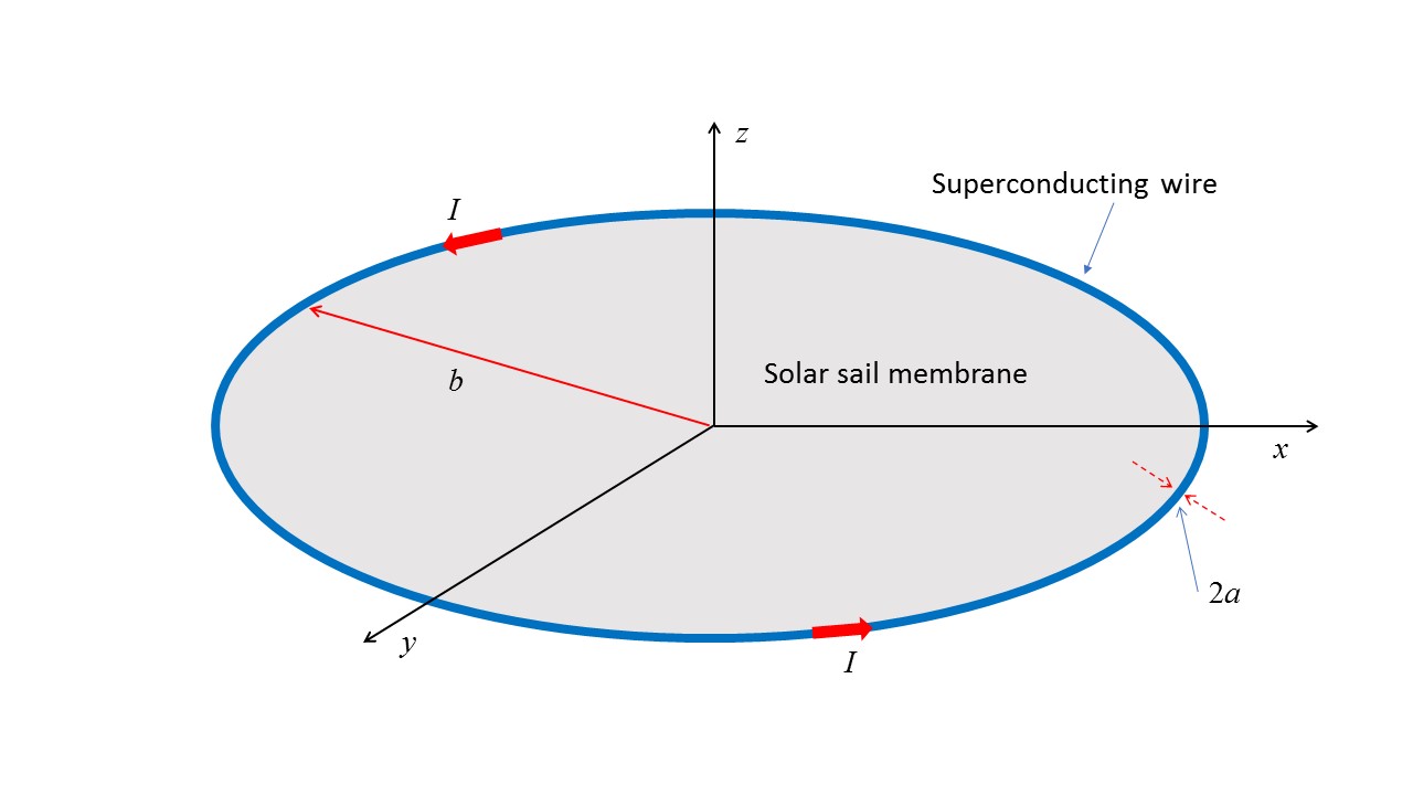
Figure 1: (Color online) A schematic of the circular solar sail of a radius $b$ attached to a superconducting circular wire of the cross-section radius $a$ currying steady-state current $I$ and laying in $x-y$ plane. The solar sail is stretched by self-forces generated by the magnetic field induced by the current-carrying wire on itself. The radius $b$ is significantly bigger than the cross-section radius of the wire $a$: $b\gg a$. The figure is not to scale.

II.1
Circular Current Wire

Let us consider a planar circular wire laying in $x-y$ plane, centered at the origin and currying steady-state current $I$ as shown in Fig. 2. We assume that the permeability $\mu=\mu_{0}$, where $\mu_{0}=4\pi\times 10^{-7}$T$\cdot$m$/$A is the permeability of the free space, in the whole space including the volume of the wire, means that both the wire and the surrounding medium are nonpermeable. If the wire is sufficiently thin and the magnetic field of interest is only in surrounding space the thickness of the wire can be neglected Landau8 . One can say that such a wire carries a linear current. Let us answer the question: can one find the force acting on the linear current due to its own magnetic field? For a system of any linear currents the vector potential $\mathbf{A}$ and magnetic induction $\mathbf{B}$ in the surrounding space become Jackson98 ; Landau8 :

$$\mathbf{A} \mathbf{=}\frac{\mu_{0}I}{4\pi}\oint\frac{d\mathbf{l}}{R},$$ (1)

$$\mathbf{B} \mathbf{=}\frac{\mu_{0}I}{4\pi}\oint\frac{d\mathbf{l\times R}}{R^{3}},$$ (2)

where for the vector potential uniqueness the Coulomb’s gauge is assumed: $div$ $\mathbf{A}=0$. In Eqs. (1) and (2) $I$ is the total current in the wire and $\mathbf{R}$ shown in Fig. 2 is the radius-vector from the current element $d\mathbf{l}$ to the point $P$, where $\mathbf{A}$ and $\mathbf{B}$ are observed. By introducing the cylindrical coordinates $r$, $\varphi$, $z$ (Fig. 2), due to axially symmetric current the vector Eq. (1) can be reduced to single scalar one:

$$A_{r}=0,\text{ }A_{z}=0,\text{ }A_{\varphi}=A(r,z).$$ (3)

For Eq. (2) we have

$$B_{r} = -\frac{1}{r}\frac{\partial}{\partial z}\left(rA_{\varphi}\right)+\frac{1}{r}\frac{\partial}{\partial\varphi}\left(A_{z}\right)=-\frac{\partial A_{\varphi}}{\partial z},\text{ }$$

$$B_{z} = -\frac{1}{r}\frac{\partial}{\partial\varphi}\left(A_{r}\right)+\frac{1}{r}\frac{\partial}{\partial r}\left(rA_{\varphi}\right)=\frac{1}{r}\frac{\partial}{\partial r}(rA_{\varphi}),\text{ }$$

$$B_{\varphi} = \frac{\partial}{\partial z}\left(A_{r}\right)-\frac{\partial}{\partial r}\left(A_{z}\right)=0.$$ (4)

It is worth noting that since we neglect the thickness of the wire, no boundary conditions at its surface need to be applied. The exact analytical solutions of Eqs. (3) and (4) are well known Landau8 ; Smythe89

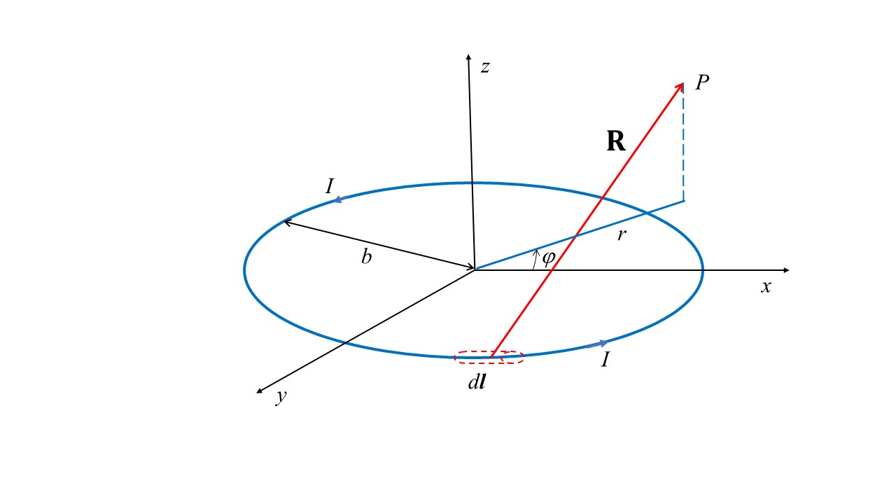
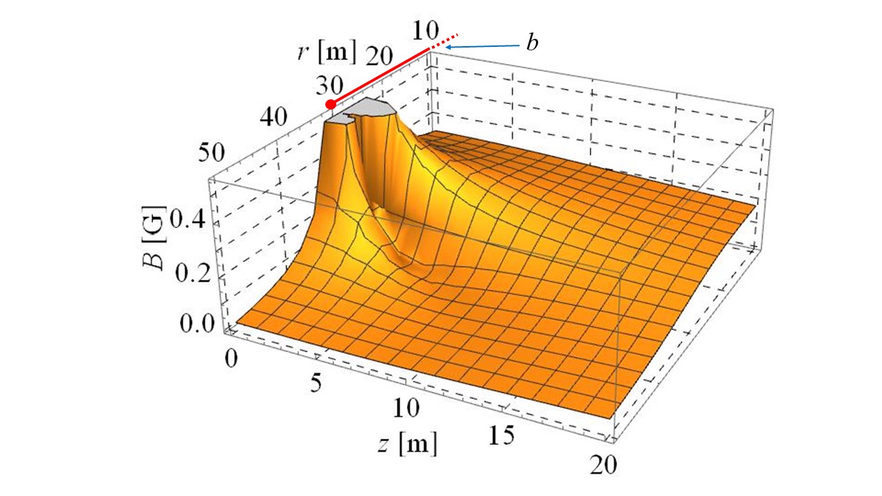
Figure 2: (Color online) Left panel: The circular wire laying in $x-y$ plane, centered at the origin and currying steady-state current $I$. The radius of the wire is $b$. $P$ indicates any point in the surrounding space where the magnetic field is induced by the wire current. Right panel: The magnetic field of the circular current-carrying wire as a function of $r$ and $z$. The logarithmic singularity of the magnetic field at $r=b$ is indicated by the point. The figure is not to scale: $b\gg a$.

$$A_{\varphi} =\frac{\mu_{0}I}{\pi k}\left(\frac{b}{r}\right)^{1/2}\left[\left(1-\frac{1}{2}k^{2}\right)K(k)-E(k)\right],$$ (5)

$$B_{r} =\frac{\mu_{0}I}{2\pi}\frac{z}{r\left[\left(b+r\right)^{2}+z^{2}\right]^{1/2}}\left[-K(k)+\frac{b^{2}+r^{2}+z^{2}}{\left(b-r\right)^{2}+z^{2}}E(k)\right],$$ (6)

$$B_{z} =\frac{\mu_{0}I}{2\pi}\frac{1}{\left[\left(b+r\right)^{2}+z^{2}\right]^{1/2}}\left[K(k)+\frac{b^{2}-r^{2}-z^{2}}{\left(b-r\right)^{2}+z^{2}}E(k)\right].$$ (7)

In Eqs. (5) - (7)

$$K(k)=\int\limits_{0}^{\pi/2}\frac{d\theta}{\sqrt{1-k^{2}\sin^{2}\theta}}\quad\text{and }\quad E(k)=\int\limits_{0}^{\pi/2}\sqrt{1-k^{2}\sin^{2}\theta}d\theta,$$ (8)

are complete elliptical integrals of the first and second kind, respectively Abramowitz ; Ryzhik . The argument $k$ of the elliptic integrals $K(k)$ and $E(k)$ is defined through $k^{2}=\frac{4br}{\left(b+r\right)^{2}+z^{2}}$ and $\theta=\frac{1}{2}\left(\varphi-\pi\right).$

It is easy to obtain well-known results given in the general physics text books for the magnetic field along $z$ axes and at the center of the circular loop. At $z$ axes ($r=0$) $B_{r}=\underset{r\rightarrow 0}{\lim}B_{r}=0$ Smythe89 ; Abramowitz and $B_{z}=\frac{\mu_{0}b^{2}I}{2\left(b^{2}+z^{2}\right)^{3/2}}$, while at the center of the circular loop $B_{r}=0$ and $B_{z}=\frac{\mu_{0}I}{2b}$. However, at the wire when $r=b$ and $z=0$, $k=1$ and, therefore, $K=\int\limits_{0}^{\pi/2}\frac{d\theta}{\cos\theta}=\ln\left|\tan\frac{\pi}{2}\right|$ diverges logarithmically, so is the magnetic field. The right panel in Fig. 2 shows an example of the distribution of magnetic field as a function of the $r$ and the distance $z$ from the $x-y$ plane. The calculations are performed for $I=1000$ A, $b=30$ m. Along the circumference of the radius $r=b$ when $z=0$ the magnetic field becomes singular. The force being a product of the current, circumference, and magnetic field becomes singular also. This result means that an attempt to calculate the force acting on the linear current due to its own magnetic field leads to the logarithmic divergence. Thus, to find the magnetic self-force on the circular wire due to its own magnetic field the cross-section of the current-caring wire can not be ignored.

II.2 Current-carrying wire self-forces

The total energy of the magnetic field of a single wire carrying a constant current $I$ is Landau8 ; Smythe89 :

$$U=\frac{1}{2}LI^{2},$$ (9)

where $L$ is the self-inductance of the wire. Again let us assume that the wire and surrounding media are nonpermeable ( $\mu=\mu_{0}$). To establish a current $I$ in the wire the change of energy of sources of electromotive force (EMF) are $-LI^{2}$ Abraham32 , so that the total free energy of the system of the EMF and wire is

$$\widetilde{U}=-\frac{1}{2}LI^{2}.$$ (10)

Thus, the total magnetic energy of the wire is

$$U=\frac{1}{2}LI^{2}=-\widetilde{U}.$$ (11)

The forces acting on the wire are Landau8 ; Jackson98

$$F_{q}=\left(-\frac{\partial\widetilde{U}}{\partial q}\right)_{I}=\left(\frac{\partial U}{\partial q}\right)_{I}=\frac{1}{2}I^{2}\left(\frac{\partial L}{\partial q}\right)_{I},$$ (12)

where $q$ is a generalized displacement of the wire and the partial derivative is taken under fixed current. These forces act as follows. For the fixed $I$ the total free energy $\widetilde{U}$ reaches the minimum. The latter means that the forces acting on the wire will tend to increase wire self-inductance. $L$ having the dimension of the length times $\mu_{0}$, is proportional to the size of the wire. Therefore, the size of the circular wire increases under the action of the magnetic self-field Landau8 .

The self-inductance of a wire can not be calculated using Newmann’s formula for the mutual inductance between $i$ and $k$ current-carrying wires Panofsky62

$$L_{ik}=\frac{\mu_{0}}{4\pi}\oint\oint\frac{d\mathbf{l}_{i}d\mathbf{l}_{k}}{r_{ik}}$$ (13)

due to the logarithmic divergence at $r_{ik}\rightarrow 0$ arising from the fact that the integrals have to be taken over the same contour. The self-inductance is much more difficult to calculate. The standard way Landau8 ; Smythe89 ; Jackson98 is to calculate the energy of the magnetic field over the whole nonpermeable space $V$ as

$$U=\frac{1}{2\mu_{0}}\int B^{2}dV$$ (14)

and then obtain $L$ from (9) as $L=\frac{2U}{I^{2}}$. The self-inductance of a current loop of the circular cross-section of radius $a$, length $C$ and a projected area $A$ (loop can be none planar) is Landau8 ; Jackson98 :

$$L\approx\frac{\mu_{0}}{4\pi}C\left(\ln\frac{\varsigma A}{a^{2}}+\frac{1}{2}\right),$$ (15)

where $a\ll\frac{C}{2\pi}$ or $a\ll A^{1/2}$and $\varsigma$ is a unitless constant of the order of 1. Equation (15) is logarithmically accurate and leads to an important conclusion: in equilibrium a flexible closed current loop of any shape will tend to take the shape spanning the maximum area $A$ for the fixed length of the wire $C$, which is the area of the circle $A=\frac{C^{2}}{4\pi}$. In other words the equilibrium shape of the flexible current-carrying wire is a perfect circle due to the magnetic force self-action. It is worth mentioning that due to inaccurate folding of the flexible wire it can be bent and have kinks and as a result, any excess rigidity in any part of the wire, will prevent wire to take the perfect circle shape. This does not contradict the conclusion above, because in the general case the free energy includes non-magnetic parts and may take a minimum with kinks remaining.

The self-inductance of the current-carrying circular wire of radius $b$ with the radius $a$ of the cross-section area when $a\ll b$ is Abraham32 ; Landau8 ; Smythe89 ; Jackson98 :

$$L=\mu_{0}b\left(\ln\frac{8b}{a}-\frac{7}{4}\right).$$ (16)

Equation (16) includes the contributions to the self-inductance due to the field inside the wire $L_{i}$ and the field outside the wire $L_{0}$. For type I superconductors and type II superconductors with the magnetic field below the first critical field, the field is expelled from the volume of the wire ($L_{i}=0$), so (16) as shown in Refs. Landau8 ; Fok becomes

$$L=\mu_{0}b\left(\ln\frac{8b}{a}-2\right).$$ (17)

For type II superconducting wire above the first critical field, the magnetic field penetrates the wire into a regular array of vortices Abrikosov and $L$ is still expressed by Eq. (16). The same is true for modern superconducting wires consisting of the regular array of individual superconducting filaments bundeled together CSWire .

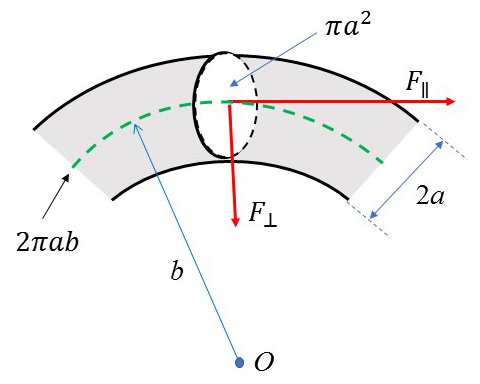
Figure 3: (Color online) A schematic for the action of forces $F_{\parallel}$ and $F_{\perp}$ on the circular wire element. The force $F_{\parallel}$ acts on the cross-section area $\pi a^{2}$ along the axis of the wire. For visibility, the cross-section of the wire is given in 3D format. The force $F_{\perp}$ acts on the area $2\pi ab$ perpendicular to the plane of the figure (shown by the dashed curve) along the normal to the axis. The figure is not to scale: $b\gg a$.

Now let us consider the self-action effect of the magnetic field on the wire. The generalized displacements of the wire are the circumference $2\pi b$ and the radius of the wire cross-section $a$. The variation of the length of the circular loop, $2\pi b$, is responsible for the force $F_{\parallel}$ acting along the axis of the wire as shown in Fig. 3, causing the tensile stress $\sigma_{\parallel}$ along it. The variation of the radius of the wire leads to the force $F_{\perp}$ normal to the axis and causing the stress $\sigma_{\perp}$ compressing the wire Landau8 . Following Ref. Landau8 and using Eqs. (12) and (16) we obtain

$$F_{\parallel} = \frac{1}{2}I^{2}\frac{\partial L}{\partial\left(2\pi b\right)}=\frac{\mu_{0}}{4\pi}I^{2}\left(\ln\frac{8b}{a}-\frac{3}{4}\right)=\pi a^{2}\sigma_{\parallel},$$ (18)

$$F_{\perp} = \frac{1}{2}I^{2}\frac{\partial L}{\partial a}=-\frac{1}{2}\frac{\mu_{0}b}{a}I^{2}=2\pi ab\sigma_{\perp},$$ (19)

where

$$\sigma_{\parallel} = \frac{\mu_{0}}{4\pi^{2}}\frac{I^{2}}{a^{2}}\left(\ln\frac{8b}{a}-\frac{3}{4}\right),$$ (20)

$$\sigma_{\perp} = -\frac{\mu_{0}}{2\pi}\frac{I^{2}}{a^{2}}.$$ (21)

The stresses $\sigma_{\parallel}$  and $\sigma_{\perp}$ will strain the wire leading to the relative elongation of the wire $\Delta b_{w}/b$, which can be obtained in the framework of the classic theory of elasticity. Following Refs. Landau8 ; Timoshenko51 ; Landau7 one can obtain

$$\frac{\Delta b_{w}}{b}=\frac{1}{E_{w}}(\sigma_{\parallel}-2\nu_{w}\sigma_{\perp}),$$ (22)

where $E_{w}$ and $\nu_{w}$ are the Young modulus of elasticity and Poisson ratio of the wire, respectively. In accordance to (20) and (21), Eq. (22) gives the change of the wire loop’s radius $b$:

$$\Delta b_{w}=\frac{\mu_{0}}{4\pi^{2}}\frac{I^{2}}{a^{2}}\frac{b}{E_{w}}\left(\ln\frac{8b}{a}-\frac{3}{4}+2\pi\nu_{w}\right).$$ (23)

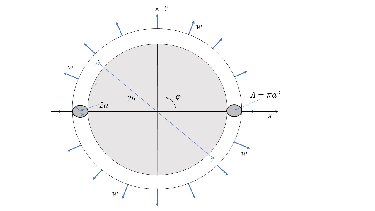
Figure 4: (Color online) A schematic for the action of uniform radial force $\omega$ acting per unit of circumferential length on the circular current-carrying wire. For visibility, the cross-section of the wire is given in 3D format. The figure is not to scale: $b\ll a$.

Let’s consider the task of finding a radial force uniformly distributed along the wire circumference which causes the change of the wire radius equal to (23). The wire under uniform radial force $w$ per unit of circumferential length is shown in Fig. 4. The final result of this classical problem is presented in Ref. Young Table 9.2, case 12 and reads:

$$\Delta b_{w}=-\frac{wb^{4}}{2\pi E_{w}\mathfrak{I}}\left[k_{1}\left(\frac{\pi^{2}\sin\theta}{2}-\sin\theta+\theta\cos\theta\right)+k_{2}\pi\left(\theta-\sin\theta-2\right)+2k_{2}^{2}\left(\pi-\theta-\sin\theta\right)\right].$$ (24)

In Eq. (24) $\mathfrak{I}=\frac{\pi a^{4}}{4}$ is the moment of inertia of the wire cross-section. In our case of the force distributed uniformly throughout the wire circumference the angle $\theta$ equals 0. In the case of $\theta=0$ the term with $k_{1}$ in the square brackets of Eq. (24) is vanishing and only the terms with $k_{2}=1-\alpha$, where $\alpha=\frac{\mathfrak{I}}{\pi a^{2}b^{2}}$ is the hoop-stress deformation factor, will survive. Substitution of the moment of inertia of the wire cross-section $\mathfrak{I}$ in the latter expression gives $\alpha=\frac{1}{4}\left(\frac{a}{b}\right)^{2}\ll 1$. Therefore, within $\left(\frac{a}{b}\right)^{2}$ accuracy Eq. (24) reads:

$$\Delta b_{w}=\frac{wb^{2}}{\pi E_{w}a^{2}}.$$ (25)

The same result for $\Delta b_{w}$ can be obtained with much less efforts following Ref. Timoshenko51 as it is illustrated in Fig. 4 by calculating tensile stress $\sigma_{t}$ in the wire cross-section due to the uniformly distributed radial force $w$

$$\sigma_{t}=\frac{1}{2\pi a^{2}}\int\limits_{0}^{\pi}wb\sin\varphi d\varphi=\frac{wb}{\pi a^{2}}$$ (26)

and equating it to the strain $\frac{\Delta b_{w}}{b}$ by considering the linear response according to the Hook’s law

$$\sigma_{t}=E_{w}\frac{\Delta b_{w}}{b}\equiv\frac{wb}{\pi a^{2}}.$$ (27)

The latter equation leads to the result (25). Equating $\Delta b_{w}$ determined by the analysis of the stress due to the magnetic self-force (23) to (25) obtained within the theory of elasticity

$$\frac{wb^{2}}{\pi E_{w}a^{2}}=\frac{\mu_{0}}{4\pi^{2}}\frac{I^{2}}{a^{2}}\frac{b}{E_{w}}\left(\ln\frac{8b}{a}-\frac{3}{4}+2\pi\nu_{w}\right),$$ (28)

one gets the magnitude of the radial uniformly distributed force $w$ per units length of the circumference

$$w=\frac{\mu_{0}}{4\pi}\frac{I^{2}}{b}\left(\ln\frac{8b}{a}-\frac{3}{4}+2\pi\nu_{w}\right).$$ (29)

Equation (29) concludes the quest for the self-force acting on the current-carrying wire due to the magnetic field induced by the current. As could be expected this force per unit of length is proportional to $\frac{\mu_{0}}{2\pi}\frac{I^{2}}{(2b)}$ as for two long wires parallel to each other which are separated by the distance 2$b$ and carrying equal current $I$. Every infinitesimally short piece of the circular wire has a counterpart parallel to it at the diameter 2$b$ away. Both pieces have the same current $I$ flow in the opposite directions and repel each other in agreement with the radially out direction of self-force $w$. Due to the circular shape of the wire the simple expression $\frac{\mu_{0}}{2\pi}\frac{I^{2}}{(2b)}$ is modified by the factor in parentheses in Eq. (29). The first term of this factor is dominant and is of the order of 10 for $b/a\sim 10^{2}-10^{4}$. The other two terms of this factor are of the order of 1 and are significantly smaller than $\ln\frac{8b}{a}$. In the equilibrium the stand-alone circular current-carrying wire under the force $w$ is balanced by the opposite elastic forces.

II.3 Stress and strain of circular membrane

Let’s consider a thin circular membrane of the radius $b$ and thickness $t$ ($t\ll b$) under a uniform distributed force $w_{m}$ per unit length of a circumference acting at the membrane edge in the radial direction as shown in Fig. 5. If the membrane is sufficiently thin, the deformation can be treated as uniform over its thickness and we have to deal with longitudinal deformations of the membrane and not with any membrane bending. For a two-dimensional case, the strain tensor is a function of $x$ and $y$ coordinates and is independent of $z$. The boundary conditions for the stress tensor on both surfaces of the membrane are

Figure 5: (Color online) Schematics for the action of the uniformly distributed radial force $w_{m}$ per unit of circumferential length of the circular membrane. ($a$) top view. ($b$) side view. The figure is not to scale: $b\gg t$.

$$\sigma_{ik}n_{k}=0,n_{k}=n_{z},i=x,y,z,$$ (30)

where $n_{k}$ is the normal vector parallel to $z-$axis and lead to

$$\sigma_{xz}=\sigma_{yz}=\sigma_{zz}=0$$ (31)

in the whole volume of the membrane when $t\ll b$ Landau7 .

The equation of equilibrium in the absence of the body forces in the two-dimensional vector form is Landau7 :

$$grad\text{ }grad\text{ }\mathbf{u-}\frac{1}{2}(1-\nu_{m})curl\text{ }curl\mathbf{u}=0,$$ (32)

where $\mathbf{u}$ is the displacement vector, $\nu_{m}$ is the membrane Poisson ratio and all the vector operators are two-dimensional. Due to the axial symmetry $\mathbf{u}$ is directed along the radius and is a function of $r$ only, so $curl$ $\mathbf{u}=0$ and Eq. (32) in polar coordinates becomes:

$$div\text{ }\mathbf{u=}\frac{1}{r}\frac{d(ru)}{dr}=const\equiv 2c$$ (33)

and gives

$$u=cr+\frac{d}{r}$$ (34)

and, therefore, the components are

$$u_{rr}=\frac{du}{dr}=c-\frac{d}{r^{2}},\text{ }u_{\varphi\varphi}=\frac{u}{r}=c+\frac{d}{r^{2}}$$ (35)

where $c$ and $d$ are some constants Handbook . In polar coordinates at $\varphi=0$ the stress $\sigma_{ik}$ and strain $u_{ik}$ tensor components are:

$$\sigma_{rr} \mathbf{=} \sigma_{xx},\text{ }\sigma_{\varphi\varphi}\mathbf{=}\sigma_{yy},\text{ }$$ (36)

$$u_{rr} \mathbf{=} u_{xx},\text{ }u_{\varphi\varphi}\mathbf{=}u_{yy}.$$ (37)

The general equations relating the strain tensor components to the stress tensor components Landau7 in our case of $\sigma_{zz}=0$ become:

$$\sigma_{xx} = \frac{E_{m}}{1-\nu_{m}^{2}}\left(u_{xx}+\nu_{m}u_{yy}\right),$$ (38)

$$\sigma_{yy} = \frac{E_{m}}{1-\nu_{m}^{2}}\left(u_{yy}+\nu_{m}u_{xx}\right),$$ (39)

where $E_{m}$ and $\nu_{m}$ are the Young modulus of elasticity and Poisson ratio of the membrane, respectively. By substituting (36) and (37) at $\varphi=0$ into (38) and (39) the stress tensor radial and angular components become:

$$\sigma_{rr} \mathbf{=} \frac{E_{m}}{1-\nu_{m}^{2}}\left(u_{rr}+\nu_{m}u_{\varphi\varphi}\right),$$ (40)

$$\sigma_{\varphi\varphi} \mathbf{=} \frac{E_{m}}{1-\nu_{m}^{2}}\left(u_{\varphi\varphi}+\nu_{m}u_{rr}\right).$$ (41)

The requirement for the deformation $u$ (34) to be finite at the membrane center and the boundary condition for $\sigma_{rr}$ (40) combined with $u_{rr}$ and $u_{\varphi\varphi}$ (35) at the membrane edge:

$$u\left(0\right)=0\text{ and }\sigma_{rr}(r=b)=\frac{w_{m}}{t}$$ (42)

determine the values of the constants $c$ and $d$:

$$c=\frac{w_{m}}{t}\frac{(1-\nu_{m})}{E_{m}},\text{ }d=0.$$ (43)

The use of the constants (43) provides the expressions for the deformation $u$ (34) and the strain (35) and the stress (40), (41) tensor components:

$$u \mathbf{=} \frac{w_{m}}{t}\frac{(1-\nu_{m})}{E_{m}}r,$$ (44)

$$u_{rr} = u_{\varphi\varphi}=\frac{w_{m}}{t}\frac{(1-\nu_{m})}{E_{m}},$$ (45)

$$\sigma_{rr} = \sigma_{\varphi\varphi}=\frac{w_{m}}{t}.$$ (46)

As expected the stress distribution (46) in the membrane deformed by the forces acting at the edge of the membrane does not depend on the elasticity constants of the membrane media Landau7 . Finally, both the radial deformation $\Delta b_{m}=u(r=b)$, the strain $\frac{\Delta b_{m}}{b}(r=b)$ and the stress $\sigma_{rm}=\sigma_{rr}(r=b)$ of the membrane edge are:

$$\Delta b_{m} \mathbf{=} \frac{w_{m}}{t}\frac{(1-\nu_{m})}{E_{m}}b,$$ (47)

$$\frac{\Delta b_{m}}{b} = \frac{w_{m}}{t}\frac{(1-\nu_{m})}{E_{m}},$$ (48)

$$\sigma_{rm} = \frac{w_{m}}{t}.$$ (49)

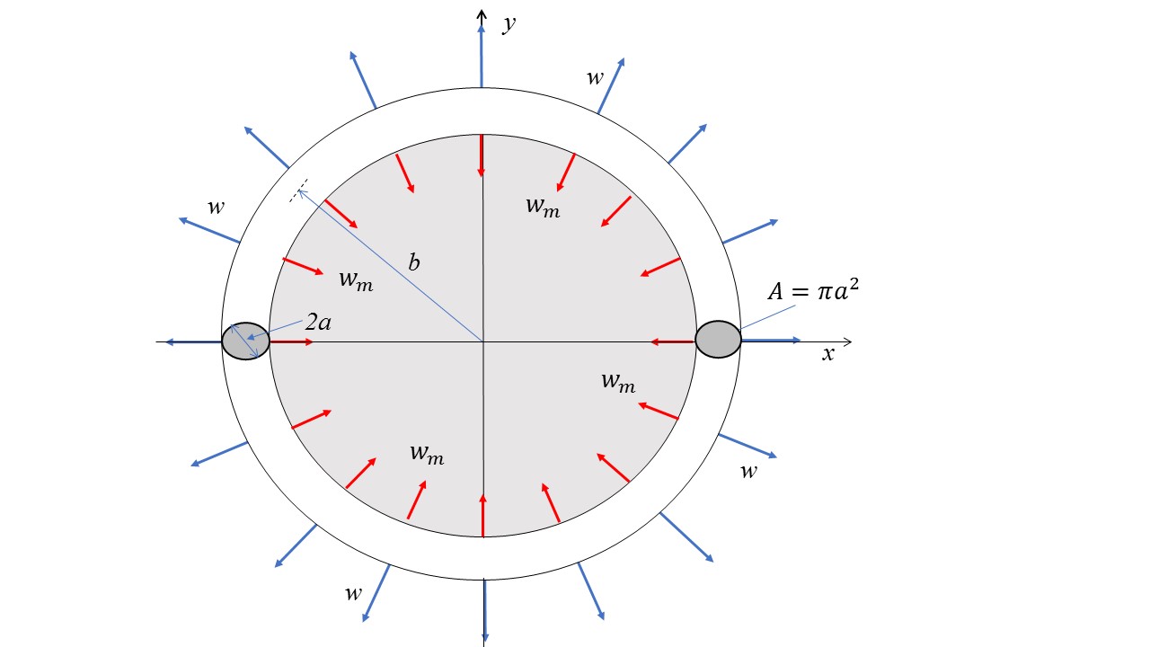
Figure 6: (Color online) Schematics for the action of uniform radial forces $w$ and $w_{m}$ per unit of circumferential length on the circular current-carrying wire. The force opposite in direction and equal in magnitude to $w_{m}$ acts on the circular membrane and is not shown. For visibility, the cross-section of the wire is given in 3D format. The figure is not to scale: $b\gg a$.

It is important to mention that all expressions in Subsec. II.3 are valid for the membrane of thickness $t$ in the shape of a ring of the external radius $b$ and internal radius of any value less than $b$ when both radii have the same center and the membrane is clamped along the internal edge. This is still the same case of two-dimensional uniform expansion as considered above.

II.4 Circular membrane attached to current-carrying wire

In the absence of the current in the wire, there are no stresses along the line of the attachment of the membrane to the wire and the membrane forms the planar disk. The current running in the wire causes the magnetic self-force $w$ acting on the wire radially out and $w_{m}$ acting on the wire from the membrane radially in as shown in Fig. 6. The latter force is in return to the stress caused by the force of the wire acting on the membrane and equal in magnitude to $w_{m}$. In the state of equilibrium we have

$$\Delta b_{w}=\Delta b_{m}.$$ (50)

The radial forces $w$ and $w_{m}$ resulting in total radial force $w-w_{m}$ has to be balanced out by the elastic forces in the wire causing the wire radius change $\Delta b_{w}$ according to (25), but with the force $w$ for stand-alone wire replaced to the force $w-w_{m}$ for the wire membrane combination. Using (25) in place of $\Delta b_{w}$ with $w$ replaced to $w-w_{m}$, and using (47) for the membrane leads (50) to

$$\frac{(w-w_{m})b^{2}}{\pi E_{w}a^{2}}=\frac{w_{m}}{t}\frac{(1-\nu_{m})}{E_{m}}b,$$ (51)

and

$$w_{m}=w\left(1+\frac{\pi a^{2}}{tb}\frac{E_{w}}{E_{m}}(1-\nu_{m})\right)^{-1}.$$ (52)

In conclusion, (48) with (52) for $w_{m}$ and (29) for $w$ allow the determination of the strain of both the wire and the membrane, $\sigma_{rm}=w_{m}/t$ (49) determines the radial stress on the membrane, and (27) with $w$ replaced by $w-w_{m}$:

$$\sigma_{t}=\frac{\left(w-w_{m}\right)b}{\pi a^{2}}$$ (53)

provides for the tensile stress of the wire.

III Results and discussion

The theory given in the previous section provides expressions to calculate different quantities related to solar sail with superconducting circular current-carrying wire such as self-inductance, magnetic energy, stress and strain. The general assumptions of applicability of these expressions are the following:

i. the materials of the wire and the membrane are nonpermeable;

ii. the radius of wire cross-section $a\ll b$, where $b$ is the radius of both the wire circular loop and membrane;

iii. both strain and stress are small and within the limit of elasticity.

The first condition is satisfied when magnetically weak materials are used, such as a superconducting wire. To satisfy the second condition the values of $\frac{a}{b}\leq 2\times 10^{-3}$ will be used. The third condition means that the stress in the wire and membrane have to be less than the yield strength of the corresponding material.

Let’s consider CP1 Polyimide films CP1 as an example of the material of the membrane used for the solar sail. The properties of CP1 are listed in Table 1. The yield strength of CP1 is not available to the authors. In general, it is much less than the Young modulus. Not knowing better one can estimate the yield strength to be greater than 10^-3 part of the Young modulus, keeping in mind that the real design decisions have to be based on experimentally measured values.

Table 1: Model parameters for the superconducting wire extracted from Refs. 45 ; 46 , and the sail membrane extracted from Refs. CP1 . $\rho_{w}$ and $\rho_{m}$, $E_{w}$ and $E_{m}$, $\nu_{w}$ and $\nu_{m}$ are the density, Young modulus, Poisson ratio, for the superconducting wire and sail membrane, respectively. $t$ is the membrane thickness.

Superconducting wire, Bi$-$2212			Sail’s membrane, CP1
$\rho_{w}$, kg/m3	$E_{w},$ Pa	$\nu_{w}$	$\rho_{m}$, kg/m3	$E_{m}$, Pa	$\nu_{m}$	$t$, m
$9.5\times 10^{3}$	$8.0\times 10^{10}$	$3.7\times 10^{-1}$	$1.43\times 10^{3}$	$2.17\times 10^{9}$	$3.40\times 10^{-1}$	$3.5\times 10^{-6}$

The High Temperature Superconducting (HTS) wire made of (Bi,Pb)₂Sr₂Ca₃Cu₂O_8-x (Bi$-$2212) with properties listed in Table 1 is chosen as the current-carrying wire. The Bi$-$2212 wire can be made into round-wire, multifilamentary strand embedded in strengthen Ag matrix CSWire ; 45 . According to the yield strength data presented in Ref. 45 it is also safe to estimate the yield strength for Bi$-$2212 superconducting wire to be greater than 10^-3 part of the corresponding Young modulus. The estimate of the engineering current density $J_{e}$, which is the current density over the whole wire cross-section including Ag matrix, is in the range of 500 A/mm² to 1000 A/mm². The rapid progress in the development of HTS wires allows to be optimistic about the commercial availability of HTS wires with even greater $J_{e}$ in near future. The current in the wire $I=\pi a^{2}J_{e}$ will be used in the calculations.

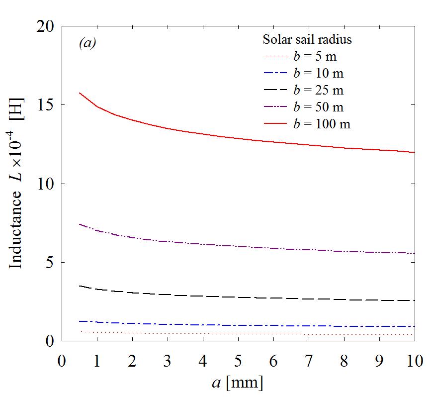
Figure 7: (Color online) Dependence of the superconducting wire self-inductance $L$ ($a$) and the total energy $U$ of the magnetic field of the wire ($b$) on the radius of the wire. Calculations performed for the engineering current $J_{e}=500$ A/mm² and a solar sail with areas from 78.5 m² to 10⁴ m².

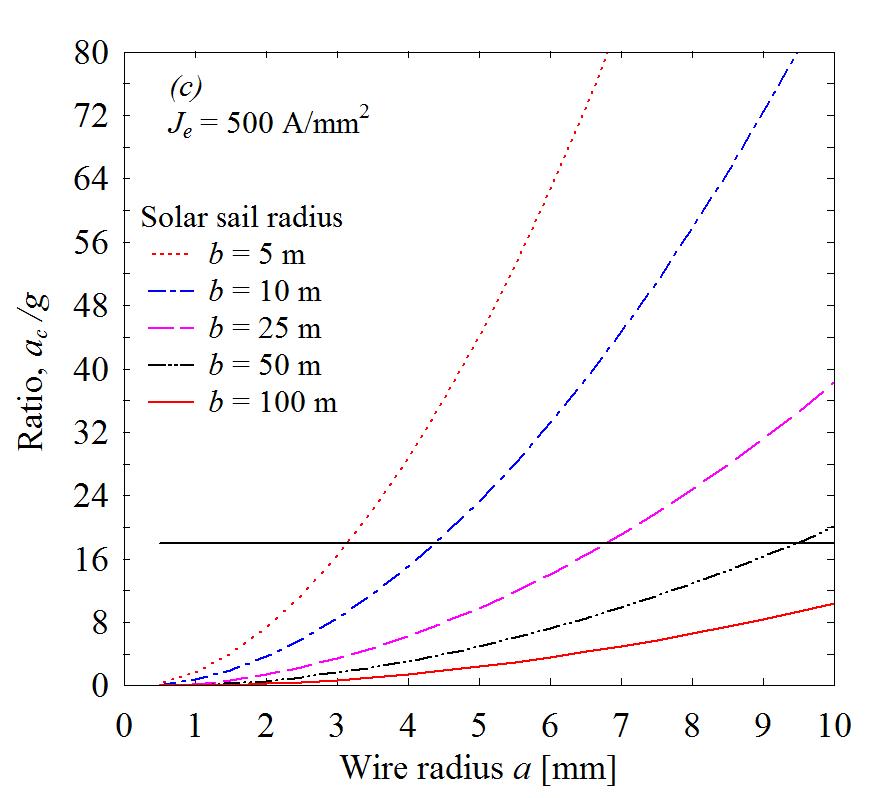
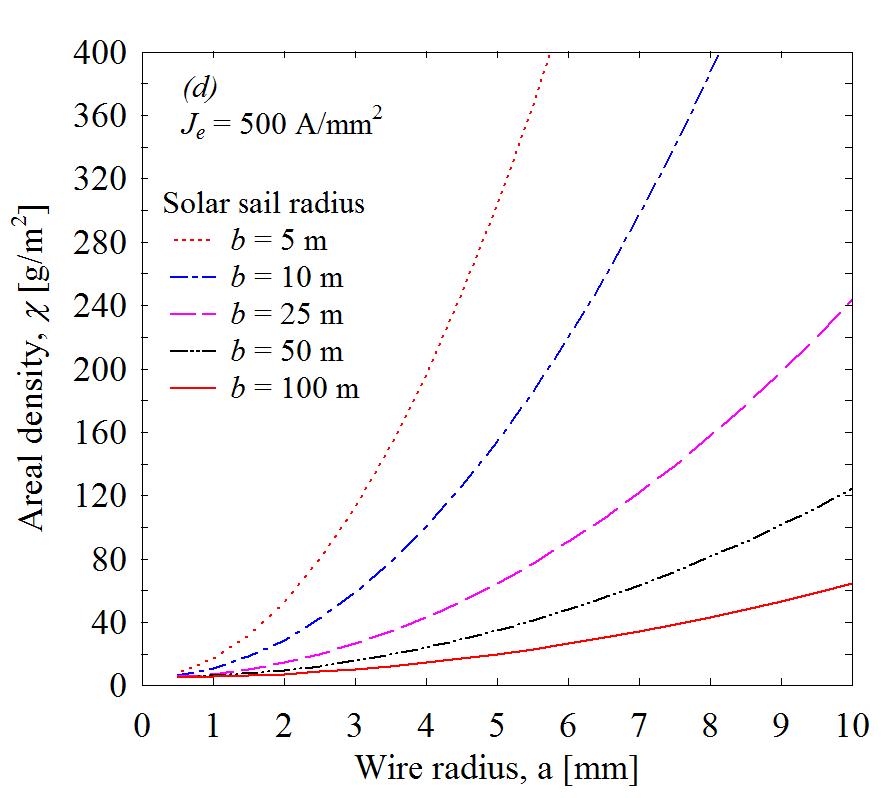
Figure 8: (Color online) Dependence of the tensile stress ($a$), membrane radial stress ($b$), the ratio $a_{c}/g$ ($c$), and arial density ($d$) on the wire radius. Calculations performed for the current density $J_{e}=500$ A/mm² and different sizes of solar sail. The horizontal line in ($c$) for the ratio $a_{c}/g$ is obtained based on the result from Ref. Deployment4 .

The expressions (16) and (9) are used to calculate the superconducting wire self-inductance $L$ and the total energy $U$ of the magnetic field of the wire carrying current $I$, respectively. The twofold of that energy $2U$ determines the minimum requirement of energy consumption of the source of EMF to establish current $I$ in the wire. The expression (29) is employed to calculate the self-force $w$ acting on the current-carrying wire due to the magnetic field induced by the current, and expression (52) gives the value of the force $w_{m}$ acting at the membrane edge. The knowledge of $w$ and $w_{m}$ is used to calculate the stress of the membrane $\sigma_{rm}$ using Eq. (49), the stress of the wire $\sigma_{t}$ using Eq. (53) and the strain $\Delta b_{m}/b$ of both Eq. (48).

Let us also introduce the ratio $a_{c}/g$ given as

$$\frac{a_{c}}{g}=\frac{\left(w-w_{m}\right)}{\rho_{w}\pi a^{2}g},$$ (54)

where $\rho_{w}$ is the wire mass density and $g=9.8$ m/s² is the acceleration due to gravity at the Earth surface. The quantity $a_{c}$ is effective acceleration equivalent to centripetal acceleration of the circular wire would it be spinning around its center with frequency

$$f=\frac{1}{2\pi}\left(\frac{a_{c}}{g}\right)^{1/2}.$$ (55)

The greater $a_{c}/g$ ratio the greater the chance of successful deployment of initially folded superconductive wire and sail membrane to the open state of circular shape. A simple analysis of the partial derivatives shows that $\sigma_{t}$, $\sigma_{rm}$, and $a_{c}/g$ are the monotonically increasing functions of radius $a$ of the wire cross-section and current density $J_{e}$. The behavior of $\sigma_{t}$ and $\sigma_{rm}$, when the radius $b$ of the wire varies is not that simple. Both $\sigma_{t}$ and $\sigma_{rm}$ exhibit a broad maximum at the same value of $b$. The position of the maximum shifts to the greater value of $b$ with an increasing value of $a$. The $a_{c}/g$ ratio behavior remains simple, it decreases monotonically with an increase of $b$.

One of the key metrics related to the performance of solar sail is the characteristic acceleration Colin ; Matloff ; Matloff2 . The characteristic acceleration is defined as $a_{0}=2\eta P_{0}/\chi$, where $0.5\leq\eta\leq 1$, $P_{0}$ is the solar radiation pressure near the Earth and $\chi=m/A$ is the areal density. In the latter expression, $m$ is the total mass of the solar sail, in our case a sum of the wire and sail membrane masses, and $A$ is the sail membrane area. While the actual sail acceleration is a function of heliocentric distance and its orientation, the characteristic acceleration allows a comparison of solar sail design concepts on an equal footing. The areal density $\chi$ is an important parameter determining the sail acceleration due to light pressure. It is easy the calculate $\chi$ for known geometry and densities of sail materials. Less $\chi$ leads to the greater sail acceleration.

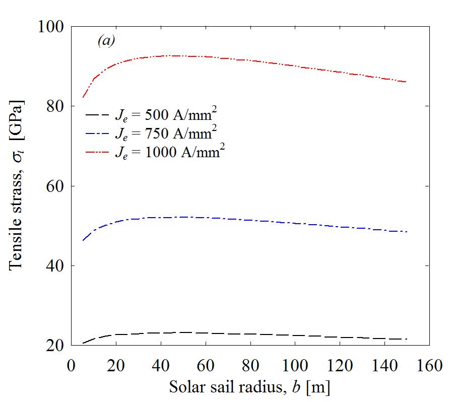
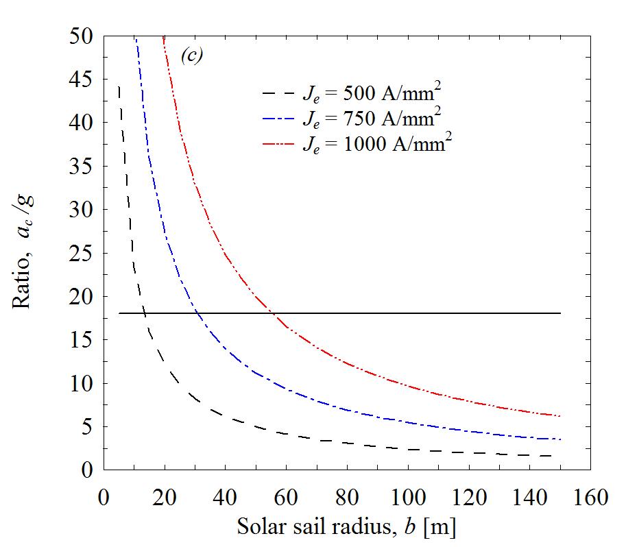
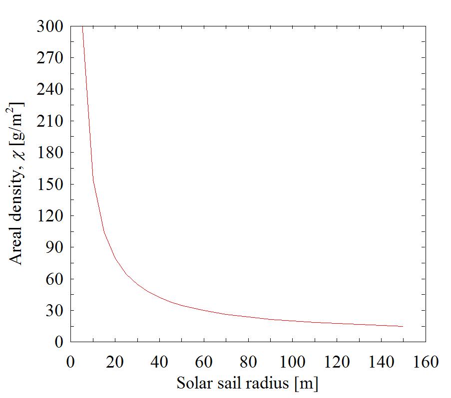
Figure 9: (Color online) Dependence of the tensile stress ($a$), membrane radial stress ($b$), the ratio $a_{c}/g$ ($c$), and arial density ($d$) on the solar sail radius. Calculations performed for the wire radius $a=5$ mm and different current densities $J_{e}$. The horizontal line in ($c$) for the ratio $a_{c}/g$ is obtained based on the result from Ref. Deployment4 .

The self-inductance $L$ and magnetic energy $U$ are presented in Fig. 7 as the function of the radius $a$ for several values of $b$. The values of $L$ are dependent only on the geometry. The values of $U$ are given for the engineering current density $J_{e}=500$ A/mm² and being dependent on the square of the current can be used to find the energy for another current density. The energy 2$U$ is of special interest giving the minimal requirement for the power supply. The superconducting wire can be operated in persistent mode with the power supply turn off after the current is established in the wire. The minimal estimate for power supply is as high as 2 MJ for the $b=10$ m sail radius with $a=10$ mm wire radius.

The dependencies of stresses $\sigma_{t}$, $\sigma_{rm}$, $a_{c}/g$ ratio, and the areal density $\chi$, respectively, on the wire radius $a$ for $J_{e}=500$ A/mm² and different fixed values of solar sail radius are presented in Fig. 8. It is clear that both the wire and membrane stresses stay within the 10^-3 range of the corresponding Young modulus for $a<7$ mm. Thus $a=7$ mm is the maximum radius of the wire cross-section to be safely used for the choice of $b<100$ m and $J_{e}=500$ A/mm². The $a_{c}/g$ ratio values range depends greatly on the value of the sail radius $b$. The greater the value of $b$ the less the range. For example, for $b=100$ m the ratio stays below 10. For $b=$ 5 m the ratio increases from 0.3 up to 63 as the wire radius $a$ changes from 0.5 mm to 6 mm.

The logical question which arises now is the following: which value of the ratio is enough to deploy the sail? Although a certain answer can be obtained only in the experiment it’s possible to compare the calculated values of $a_{c}/g$ ratio with the equivalent estimate based on the successful ground demonstration of the spinning sail deployment by Jet Propulsion Laboratory Deployment4 . The data provided in Ref. Deployment4 for the spinning frequency 200 RPM or more of the sail of 0.8 m in diameter gives the estimate of the ratio of centripetal acceleration over the acceleration due to gravity equal to 18 or more. The calculated $a_{c}/g$ ratio presented in Fig. 8c exceeds this estimate for the certain range of wire radius $a$ values for a choice of sail radius $b<$ 25 m. For example, the ratio is well above the estimate for $b=10$ m as $a>4$ mm. As is expected the areal density increases with the increase of the wire radius and decrease of the sail radius. This means that for the certain choice of sail size the less value of wire radius is preferable as far as the $a_{c}/g$ ratio allows the sail to be deployed and the wire and the sail membrane stay within the limit of elasticity. For $J_{e}=$500 A/mm² and $b=10$ m the choice of $a=5$ mm is close to an optimal with $\chi=155$ g/m².

Figure 9 presents the stresses $\sigma_{t}$, $\sigma_{rm}$, $a_{c}/g$ ratio, and the areal density $\chi$, respectively, as function of sail radius $b$ for the different current densities $J_{e}$ and the fixed value of the wire radius $a=5$ mm. It is clear that both the wire and membrane stresses stay within the 10^-3 range of the corresponding Young modulus for $J_{e}\leq 750$ A/mm². As expected, both the $a_{c}/g$ and $\chi$ monotonically decrease with the increase of the sail radius $b$. For fixed $b$ the increase of current density leads to increase of the $a_{c}/g$ without any effect of the areal density. This means that the reasonable values of $b$ increase with the increase of the current density. For example, for the chosen values of $a=5$ mm and $J_{e}=750$ A/mm² the solar sail radius can be as big as 25 m with $\chi\sim 64$ g/m².

It is worth noting that we performed the same calculations for the dependencies of stresses on the wire and solar sail radii for the most widely used low temperature superconductor Nb$-$Ti. The similar results were obtained.

IV Concluding remarks

The theory of circular solar sail attached to superconducting current-carrying wire is developed within the framework of classical electrodynamics and theory of elasticity. We obtained the analytical expressions that can be applied to a wide range of the materials of both the wire and sail membrane. The presented numerical example demonstrates the power of the developed theory to provide sound estimates of the stresses of the solar sail with attached superconducting circular current-carrying wire along with the power requirements solely based on the geometry, engineering current density and elastic properties of the materials used.

It is possible to imagine different options of the sail attachment to the useful load, which can represent the spacecraft itself. The theory presented is directly applicable to the case when the sail is in the shape of a ring and is clamped along the internal edge to the load having a circular cross section in the plane of the sail. Another option is the sail in the shape of the rosette of the daisy. In this case, the leaves of the rosette are sails of the same size arranged regularly around the base represented by a load of circular cross section. Each leave sail is the circular sail with superconducting current-carrying wire around. It is not necessary to have all the leave sails in the same plane, each of them can have its own orientation in space allowing to steer the load. Moreover, one can envision that the orientation of each leave can be changed to achieve the needed maneuver. Arrangement of multiple sails in daisy-like shape will require further advance of the presented theory to take into account the effects of mutual inductance of the sails. The case of the load attached via flexible tethers to the wire of the sail at regular length intervals will require the theory advance to take into account the action of the forces at the points of tethers attachment. One can operate the sail in persistent mode when the superconducting wire is detached from the power supply after the current is established, and also dump the current and close the sail using the lightweight flexible tethers and re-open it by injecting the current in the wire as needed. This kind of close-open operating mode can be quite useful in the case of daisy shaped sail, when all the leave sails are in the same plane, but the needed maneuver can be achieved by closing one or more leave sails and later re-opening them.

Today all launched solar sails have a square shape and such design is related to the deployment mechanism. The world’s first interplanetary solar sail, – the IKAROS, successfully deployed its 196 m² sail in 2010. NASA’s first solar sail deployed in low earth orbit was NanoSail-D which had 9.3 m² of light-reflecting catching surface and the LightSail-2 on July 23, 2019, deployed its 32 m² solar sail. For comparison, our calculations show that the sail of $\sim 1,963$ m² area (25 m radius) with the attached wire of 5 mm cross-section radius is expected to be deployed by the current in the wire of the engineering density 750 A/mm² with $a_{c}/g=22$ and $\chi=64$ g/m². This sail is even bigger than NASA’s Solar Cruiser, a mission launching in 2025 to test a giant sail measuring 1,650 m².

To conclude our calculations demonstrate the feasibility of the proposed idea for the deployment and stretching of the circular solar sail constructed as the superconducting current loop attached to the thin circular membrane. At this point, the sound experimental study is needed to find out the level of the feasibility of the proposed idea for the future of the deep space exploration by means of the light pressure propellent.

- (1) R. M. Zubrin and D. G. Andrews, Magnetic sails and interplanetary travel. J. Spacecr Rockets 28, 197–203 (1991).
- (2) R. M. Zubrin, The use of magnetic sails to escape from low earth orbit. J. Br. Interplanet. Soc. 46, 3–10 (1993).
- (3) P. Janhunen, Electric Sail for Spacecraft Propulsion, J. Propul. Power, 20, 763 (2004).
- (4) P. Janhunen and A. Sandroos, Simulation study of solar wind push on a charged wire: basis of solar wind electric sail propulsion, Ann. Geophys. 25, 755–767 (2007).
- (5) J. C. Maxwell, A Treatise on Electricity and Magnetism. Oxford University Press, Oxford, 1873.
- (6) P. N. Lebedev, 1901. First experimental evidence for pressure of the light on the solid bodies. Annalen der Physik, Leipzig: Barth 6, 433–458 (1901).
- (7) E. F. Nichols and G. F. Hull, A preliminary communication on the pressure of heat and light radiation, Phys. Rev. 13, 307 (1901).
- (8) R. F. Nichols and G. F. Hull, Pressure due to radiation. Physical Review (Series I) XVII, 26–50 (1903).
- (9) Ya. M. Perelman, 1915. Mezhplanetnie puteshestvia, in: Russian (Interplanetary Journeys). Publisher P.P. Soykin, Peterburg, 1915.
- (10) F. A. Tsander, F. A. Zander, Technika i Zhizn, 13, 15 (1924). Iz nauchnogo nasledia, in Russian, (From a scientific heritage), Nauka, Moscow, 1967; Selected Papers, in Russian, Zinatne, Riga, 1977.
- (11) R. W. Parkinson, H. M. Jones, and I. I. Shapiro, Effects of solar radiation pressure on earth satellite orbits, Science 131, 920 (1960).
- (12) P. Musen, 1960. The Influence of the solar radiation pressure on the motion of an artificial satellite, J. Geophys. Res. 65, 1391 (1962).
- (13) P. Musen, R. Bryant, and A. Baili, Perturbations in Perigee Height of Vanguard I, Science 131, 935 (1960).
- (14) G. F. Pezditz, Erectable space structures-ECHO Satellites, NASA N62-12545 (1962).
- (15) I. I. Shapiro and H. M. Jones, Perturbations of the orbit of the Echo balloon, Science, 132, 1484 (1960).
- (16) Y. Tsuda, O. Mori, R. Funase, H. Sawada, T. Yamamoto, T. Saiki, T. Endo, and J. I. Kawaguchi, Flight status of IKAROS deep space solar sail demonstrator. Acta Astronautica 69, 833–840 (2011).
- (17) R. Ya. Kezerashvili, Solar sailing: Concepts, technology, and missions, Adv. Space Res. 48, 1683 (2011).
- (18) J. M. Fernandez, V. J. Lappas, A. J. Daton-Lovett, Completely stripped solar sail concept using bi-stable reeled composite booms. Acta Astronautica 69, 78–85 (2011).
- (19) M. Salama, C. White, and R. Leland, Ground demonstration of a spinning solar sail deployment concept. J. Spacecraft Rock. 40, 9–14 (2003) https://doi.org/10.2514/2.3933.
- (20) B. Vatankhahghadim and C. J. Damaren, Solar sail deployment dynamics, Adv. Space Res. 67, 2746–2756 (2021).
- (21) V. Parque, W. Suzaki, S. Miura, A.Torisaka, T. Miyashita, and M. Natori, Packaging of thick membranes using a multi-spiral folding approach: Flat and curved surfaces, Adv. Space Res. 67, 2589–2612 (2021).
- (22) L. T. Hibbert and H. W. Jordaan, Considerations in the design and deployment of flexible booms for a solar sail, Adv. Space Res. Adv. Space Res. 67, 2716–2726 (2021).
- (23) A. Boschetto, L. Bottini, G. Costanza, and M. E. Tata, Shape memory activated self-deployable solar sails: small-scale prototypes manufacturing and planarity analysis by 3D laser scanner, Actuators 8, 38 (2019).
- (24) A. Boschetto, L. Bottini, G. Costanza, and M. E. Tata, A novel self-deployable solar sail system activated by shape memory alloys, Aerospace 6, 78 (2019).
- (25) R. Ya. Kezerashvili, O. L. Starinova, A. S. Chekashov, and D. J. Slocki, A torus-shaped solar sail accelerated via thermal desorption of coating, Adv. Space Res. 67, 2577–2588 (2021).
- (26) J. H. Jeans, The Mathematical Theory of Electricity and Magnetism, 5th Edition, Cambridge University Press, London, UK, 1927.
- (27) A. Sommerfeld, Electrodynamics, Academic Press, New York, USA, 1952.
- (28) M. Abraham and R. Becker, Electricity and Magnetism, Blackie & Son Ltd, Glasgow, UK, 1932.
- (29) W. K. H. Panofsky and M. Phillips, Classical Elecricity and Magnetism, 2nd Edition, Addison-Wesley Pub. Com. Inc. Massachusetts, USA, 1962.
- (30) L. D. Landau and E. M. Lifshitz, Electrodynamics of Continuos Media, 2nd Edition, Revised and Enlarged, Pergamon Press, Oxford, UK, 1984.
- (31) W. R. Smythe, Static and Dymanics Electricity, 3Edition, Taylor & Francis, Bristol, Pennsylvania, USA, 1989.
- (32) W. Greiner, Classical Electrodynamics, Springer-Verlag, New York, Inc, 1998.
- (33) J. D. Jackson, Classical Electrodynamics, 3rd Edition, John Wiley & Sons, Inc., New York, USA, 1998.
- (34) S. Timoshenko, Strength of Materials, Part I, Elementary Theory and Problems, 2nd Edition, D. Van Nostrand Com., 1940.
- (35) L. D. Landau and E. M. Lifshitz, Theory of Elasticity, 3rd English Edition, Revised and Enlarged, Pergamon Press, Oxford, UK, 1986.
- (36) V. S. Boyko, R. I. Garber, and A. M. Kossevich, Reversible Crystal Plasticity, American Institute of Physics, New York, USA, 1994.
- (37) Handbook of Mathematical Functions With Formulas, Graphs, and Mathematical Tables, edited by M. Abramowitz and I. A. Stegun, NBS Applied Mathematics Series 55, National Bureau of Standards, Washington, 1964.
- (38) I. S. Gradshteyn and I. M. Ryzhik, Table of Integrals, Series, and Products, 7th Edition, Elsevier, Amsterdam, 2007.
- (39) V. A. Fok, Skin-effect in a ring of a circular section, Physicalische Zeitschrift der Sowjetunion, Phys. Zs. Sowjet. 1, 215-236 (1932).
- (40) A. A. Abrikosov, The magnetic properties of superconducting alloys, J. Phys. Chem. Solids, 2, 199-208 (1957).
- (41) G. De Marzi, L. Muzzi, and P. J. Lee, Superconducting Wires and Cables: Materials and Processing. Elsevier, 2016.
- (42) W. C. Young and R. G. Budynas, Roark’s Formulas for Stress and Strain, 7th Edition, McGraw-Hill, New York, USA, 2002.
- (43) A. D. Polyanin and V. F. Zaitsev, Handbook of Ordinary Differential Equations, CRC Press, Taylor & Francis, Boca Raton, USA, 2018.
- (44) A. Peloni, D. Barbera, S. Laurenzi, C. Circi, Dynamic and structural performances of a new sailcraft concept for interplanetary missions, Scientific World Journal, Volume 2015, Article ID 714371, 14 pages http://dx.doi.org/10.1155/2015/714371.
- (45) X. F. Lu, N. Cheggour, T. C. Stauffer, C. C. Clickner, L. F. Goodrich, U. Trociewitz, D. Myers, and T. G. Holesinger, Electromechanical Characterization of Bi-2212 Strands, IEEE Transactions on Applied Superconductivity 21, 3086 (2011).
- (46) American Institute of Physics Handbook, Third Edition, McGray-Hill, 1972.
- (47) C. R. McInnes, Solar Sailing - Technology, Dynamics and Mission Applications. Springer, Praxis Publishing, Chichester UK, 1999.
- (48) G. L. Matloff, Deep Space Probes: To the Outer Solar System and Beyond. Springer/Praxis Books 2005.
- (49) G. Vulpetti, L. Johnson, and G. L. Matloff, Solar Sails - A Novel Approach to Interplanetary Travel. Copernicus Books, 2008.