A First Detection of the Connected 4-Point Correlation Function of Galaxies Using the BOSS CMASS Sample

Abstract

We present an $8.1\sigma$ detection of the non-Gaussian 4-Point Correlation Function (4PCF) using a sample of $N_{\rm g}\approx 8\times 10^{5}$ galaxies from the BOSS CMASS dataset. Our measurement uses the $\mathcal{O}(N_{\rm g}^{2})$ NPCF estimator of Philcox et al. (2021), including a new modification to subtract the disconnected 4PCF contribution (arising from the product of two 2PCFs) at the estimator level. This approach is unlike previous work and ensures that our signal is a robust detection of gravitationally-induced non-Gaussianity. The estimator is validated with a suite of lognormal simulations, and the analytic form of the disconnected contribution is discussed. Due to the high dimensionality of the 4PCF, data compression is required; we use a signal-to-noise-based scheme calibrated from theoretical covariance matrices to restrict to $\sim$ $100$ basis vectors. The compression has minimal impact on the detection significance and facilitates traditional $\chi^{2}$-like analyses using a suite of mock catalogs. The significance is stable with respect to different treatments of noise in the sample covariance (arising from the limited number of mocks), but decreases to $4.7\sigma$ when a minimum galaxy separation of $14\,h^{-1}\mathrm{Mpc}$ is enforced on the 4PCF tetrahedra (such that the statistic can be modelled more easily). The detectability of the 4PCF in the quasi-linear regime implies that it will become a useful tool in constraining cosmological and galaxy formation parameters from upcoming spectroscopic surveys.

I Introduction

The detection of a non-Gaussian signature in the early Universe would be a smoking gun for many inflation models [e.g., 1]. Despite a number of searches, no evidence has been found for primordial non-Gaussianity in the Cosmic Microwave Background (CMB) [2]. Given that its signal in the CMB is found primarily on large, cosmic variance dominated scales, the situation is unlikely to change dramatically in the near future [3]. With the upcoming influx of data from spectroscopic surveys such as DESI [4] and Euclid [5], it is natural to expect that large-scale structure (LSS) will soon become a key dataset with which to probe such signatures.

At late times, there is an additional source of non-Gaussianity: structure growth induced by gravitational evolution [e.g., 6]. Far from simply being a contaminant in the search for signatures from early-Universe physics, gravitational non-Gaussianities provide significant information on cosmological parameters such as the growth rate, neutrino masses, and modified gravity parameters [e.g., 7, 8, 9, 10]. As such, measuring non-Gaussian statistics such as the higher-order $N$-Point Correlation Functions (NPCFs) or their Fourier-space equivalents (polyspectra) provides a powerful approach with which to enhance cosmological analyses, capturing information shifted out of the Gaussian two-point function due to gravitational evolution [11]. Furthermore, it is vital to understand the late-time contributions to these statistics if we wish to use them to extract constraints on primordial non-Gaussianities [12, 13].

A number of recent analyses have included the simplest non-Gaussian statistic; the 3-Point Correlation Function (3PCF) [14, 15], or bispectrum [16, 17, 18, 19, 20]. This has been facilitated by fast algorithms for computing such statistics [e.g., 21, 22, 23, 24, 25, 26, 27, 28, 29], as well as the development of theory models for the galaxy 3PCF [30] and bispectrum [e.g., 31, 32, 33, 34, 35, 36, 37], though the latter is still in its infancy. The additional information contained within the 3PCF has sharpened cosmological parameter constraints [20, 38, 18], particularly through the Baryon Acoustic Oscillation (BAO) feature [39, 17], and probed the relative velocity of baryons and dark matter [40, 15].

In this work, we focus on the next non-Gaussian statistic: the 4-Point Correlation Function (4PCF). This has been scarcely considered in the literature; a handful of works explore its estimation [25, 41, 42], and, for the matter field, its modelling [43, 44], and projected parameter constraints [45]. Besides sharpening constraints on $\Lambda$CDM parameters, the 4PCF can also be used to test new physics such as parity violation [46]; this will be considered in depth in [47]. Unlike the 2PCF and 3PCF, the 4PCF contains both an intrinsic (‘connected’) four-point function, and a disconnected piece, which depends on the product of two 2PCFs (as sketched in Fig. 1). Given that the latter contains only information degenerate with that in the 2PCF, it is important to separate the two contributions. Here, our goal is to extract only the connected 4PCF, unlike previous work [41].

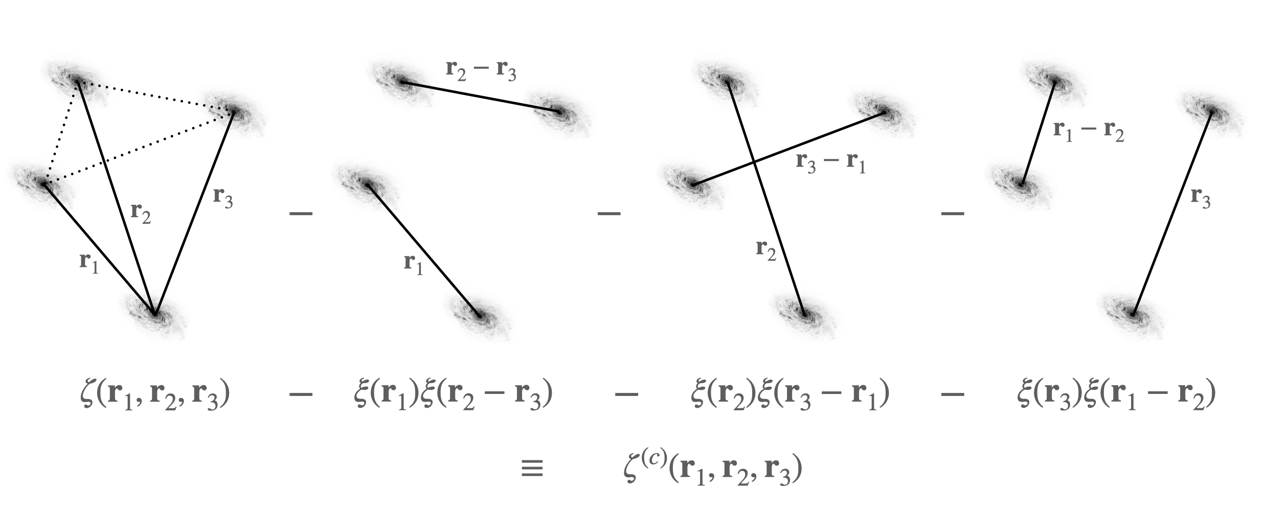
Figure 1: Schematic of the connected galaxy 4PCF. The first cartoon shows the contribution of a single tetrahedron of galaxies to the full 4PCF, $\zeta(\bm{r}_{1},\bm{r}_{2},\bm{r}_{3})$, which is parametrized by the separations of three secondary galaxies from a given primary (at the base of the tetrahedron). The complete statistic can be formed by summing over all such tetrahedra of galaxies; in practice, we use a spherical harmonic decomposition which is considerably more efficient [48]. In the second through fourth diagrams, we show the contributions to the disconnected 4PCF, arising from products of two 2PCFs, $\xi(\bm{r})$. The complete statistic may be computed by iterating over pairs of galaxies. The difference between the full and disconnected configurations gives the connected 4PCF, $\zeta^{(\rm c)}(\bm{r}_{1},\bm{r}_{2},\bm{r}_{3})$, which is the quantity of interest in this work.

Performing a 4PCF analysis comes with a number of challenges. Firstly, estimation of the statistic is non-trivial, with naïve approaches having $\mathcal{O}(N_{\rm g}^{4})$ complexity when applied to a dataset containing $N_{\rm g}$ galaxies. Here, we apply the recently-proposed $\mathcal{O}(N_{\rm g}^{2})$ NPCF estimators [48, 49] which achieve a significant speed-boost by projecting the statistic onto a separable angular basis obtained from the theory of angular momentum addition [50]. Coupled with a new procedure for removing the disconnected component at the estimator level, this allows the connected isotropic 4PCF to be computed in only a few tens of CPU-hours, including survey geometry corrections. Furthermore, the dimensionality of the 4PCF is large, making traditional mock-based analyses difficult. To ameliorate this, we use the signal-to-noise based compression scheme of [31], which greatly reduces the number of bins with minimal impact on the detection significance. A key part of the compression scheme is a smooth approximation to the 4PCF covariance; for this purpose, we make use of analytic NPCF covariances derived in [51] under certain simplifying assumptions. This facilitates a traditional $\chi^{2}$ analysis calibrated using realistic mock catalogs, allowing our 4PCF detection significance to be quantified, albeit under the assumption of a Gaussian likelihood.

The remainder of this paper is structured as follows. §II provides a summary of the 4PCF estimator introduced in [48], before we discuss the modifications required to remove the disconnected 4PCF in §III. Using a suite of lognormal simulations and an analytic form for the disconnected 4PCF, the estimator is tested in §IV. In §V, we outline our data compression scheme, with the data, simulations and analytic covariance being introduced in §VI. The results of our analysis are presented in §VII, before we conclude in §VIII. Appendices A, B & C present various useful results and consistency checks. Our main results are displayed in Figs. 3 & 5, respectively showing a selection of the BOSS 4PCF measurements, and the detection significance.

Throughout this work we use the fiducial cosmology $\{\Omega_{m}=0.31,\Omega_{b}h^{2}=0.022,h=0.676,\sigma_{8}=0.8,n_{s}=0.96,\sum m_{\nu}=0.06\,\mathrm{eV}\}$ as in [52]; the neutrino sector is modeled as a single massive neutrino. Furthermore, we adopt the Fourier conventions $P(\bm{k})=\int d\bm{r}\,e^{-i\bm{k}\cdot\bm{r}}\xi(\bm{r})\leftrightarrow\xi(\bm{r})=\int_{\bm{k}}P(\bm{k})e^{i\bm{k}\cdot\bm{r}}\xi(\bm{r})$ for power spectrum $P(\bm{k})$ and 2PCF $\xi(\bm{r})$, denoting $(2\pi)^{-3}\int d\bm{k}\equiv\int_{\bm{k}}$. The main analysis pipeline of this work is available on GitHub.

II The Full 4PCF Estimator

We begin with a summary of the isotropic 4PCF estimator of [48, 49], including discussion of the relevant angular basis [50]. Note that this estimates both the disconnected and connected 4PCF; the removal of the former piece is described in §III. All estimators are implemented in the public encore code, written in C++ and cuda.

II.1 Idealized Estimator

The 4PCF is defined as a statistical expectation of four copies of the density field, $\delta$:

$$\zeta(\bm{r}_{1},\bm{r}_{2},\bm{r}_{3})\equiv\left\langle{\delta(\bm{s})\delta(\bm{s}+\bm{r}_{1})\delta(\bm{s}+\bm{r}_{2})\delta(\bm{s}+\bm{r}_{3})}\right\rangle.$$ (1)

By definition, the isotropic 4PCF depends only on the shape of the quadrilateral defined by the separation vectors $\{\bm{r}_{1},\bm{r}_{2},\bm{r}_{3}\}$ (as in Fig. 1), and not on its spatial position or orientation. As shown in [50], any isotropic function of $(N-1)$ coordinates in 3D can be expanded in terms of the following basis vectors:

$$\mathcal{P}_{\Lambda}(\hat{\bm{r}}_{1},\ldots,\hat{\bm{r}}_{N-1}) = \sum_{M}C_{\Lambda}^{M}\;Y_{\ell_{1}}^{m_{1}}(\hat{\bm{r}}_{1})\cdots Y_{\ell_{N-1}}^{m_{N-1}}(\hat{\bm{r}}_{N-1}),$$ (2)

where $\Lambda$ and $M$ are sets of total and projected angular momentum indices respectively, $C_{\Lambda}^{M}$ is a coupling matrix, and $Y_{\ell}^{m}(\hat{\bm{r}})$ is a spherical harmonic. Since the dependence of (2) on the unit vectors $\hat{\bm{r}}_{i}$ is separable, the $\mathcal{P}_{\Lambda}$ functions offer a convenient basis for efficient computation of the isotropic NPCFs [48]. For $N=4$, the basis becomes

$$\boxed{\mathcal{P}_{\ell_{1}\ell_{2}\ell_{3}}(\hat{\bm{r}}_{1},\hat{\bm{r}}_{2},\hat{\bm{r}}_{3})=(-1)^{\ell_{1}+\ell_{2}+\ell_{3}}\sum_{m_{1}=-\ell_{1}}^{\ell_{1}}\sum_{m_{2}=-\ell_{2}}^{\ell_{2}}\sum_{m_{3}=-\ell_{3}}^{\ell_{3}}\begin{pmatrix}{\ell_{1}}&{\ell_{2}}&{\ell_{3}}\\ {m_{1}}&{m_{2}}&{m_{3}}\end{pmatrix}Y_{\ell_{1}}^{m_{1}}(\hat{\bm{r}}_{1})Y_{\ell_{2}}^{m_{2}}(\hat{\bm{r}}_{2})Y_{\ell_{3}}^{m_{3}}(\hat{\bm{r}}_{3}),}$$ (3)

where the $2\times 3$ matrix is a Wigner 3-$j$ symbol [53, §34.3] and the basis depends on three angular momentum indices $\{\ell_{1},\ell_{2},\ell_{3}\}$, which (a) can take only non-negative integer values, and (b) must satisfy the triangle condition $|\ell_{1}-\ell_{2}|\leq\ell_{3}\leq\ell_{1}+\ell_{2}$. (3) is closely related to the tripolar spherical harmonic (TriPoSH) basis functions of zero total angular momentum [54]. The isotropic 4PCF can be expanded in this basis as

$$\zeta(\bm{r}_{1},\bm{r}_{2},\bm{r}_{3})=\sum_{\ell_{1}\ell_{2}\ell_{3}}\zeta_{\ell_{1}\ell_{2}\ell_{3}}(r_{1},r_{2},r_{3})\mathcal{P}_{\ell_{1}\ell_{2}\ell_{3}}(\hat{\bm{r}}_{1},\hat{\bm{r}}_{2},\hat{\bm{r}}_{3});$$ (4)

by orthogonality, the coefficients (hereafter denoted ‘multiplets’) can be obtained via

$$\zeta_{\ell_{1}\ell_{2}\ell_{3}}(r_{1},r_{2},r_{3}) = \int d\hat{\bm{r}}_{1}d\hat{\bm{r}}_{2}d\hat{\bm{r}}_{3}\,\zeta(\bm{r}_{1},\bm{r}_{2},\bm{r}_{3})\,\mathcal{P}^{*}_{\ell_{1}\ell_{2}\ell_{3}}(\hat{\bm{r}}_{1},\hat{\bm{r}}_{2},\hat{\bm{r}}_{3}).$$ (5)

In this work, we assume the 4PCF to be invariant under the parity transform $\{\bm{r}_{1},\bm{r}_{2},\bm{r}_{3}\}\rightarrow\{-\bm{r}_{1},-\bm{r}_{2},-\bm{r}_{3}\}$ (i.e. parity-even); this implies that the multiplets $\zeta_{\ell_{1}\ell_{2}\ell_{3}}$ are non-zero only for even $\ell_{1}+\ell_{2}+\ell_{3}$ [48]. Furthermore, the condition ensures that both the basis functions and the 4PCF coefficients are real. The parity-odd case will be discussed in [47]; standard model physics is not expected to generate such a contribution on large scales.

Via the ergodic principle, the full 4PCF may be estimated as a spatial integral over four copies of $\delta$, assuming statistical homogeneity:

$$\hat{\zeta}(\bm{r}_{1},\bm{r}_{2},\bm{r}_{3})=\frac{1}{V}\int d\bm{s}\,\delta(\bm{s})\delta(\bm{s}+\bm{r}_{1})\delta(\bm{s}+\bm{r}_{2})\delta(\bm{s}+\bm{r}_{3}),$$ (6)

where $V$ is the survey volume. In combination with (5), this gives an estimator for the 4PCF multiplets in radial bins $\{a,b,c\}$:

$$\hat{\zeta}^{abc}_{\ell_{1}\ell_{2}\ell_{3}}=\frac{1}{V}\int d\bm{s}\,d\bm{r}_{1}d\bm{r}_{2}d\bm{r}_{3}\,\delta(\bm{s})\delta(\bm{s}+\bm{r}_{1})\delta(\bm{s}+\bm{r}_{2})\delta(\bm{s}+\bm{r}_{3})\,\mathcal{P}^{*}_{\ell_{1}\ell_{2}\ell_{3}}(\hat{\bm{r}}_{1},\hat{\bm{r}}_{2},\hat{\bm{r}}_{3})\frac{\Theta^{a}(r_{1})}{v_{a}}\frac{\Theta^{b}(r_{2})}{v_{b}}\frac{\Theta^{c}(r_{3})}{v_{c}},$$ (7)

where the binning functions $\Theta^{u}(r)$ are unity if $r=|\bm{r}|$ is in bin $u$ and zero else, and $v_{u}$ is the bin volume. The estimator can be factorized:

$$\hat{\zeta}^{abc}_{\ell_{1}\ell_{2}\ell_{3}} = \frac{1}{V}\int d\bm{s}\,\delta(\bm{s})\sum_{m_{1}m_{2}m_{3}}\begin{pmatrix}{\ell_{1}}&{\ell_{2}}&{\ell_{3}}\\ {m_{1}}&{m_{2}}&{m_{3}}\end{pmatrix}\left[\frac{1}{v_{a}}\int d\bm{r}_{1}\,\delta(\bm{s}+\bm{r}_{1})Y_{\ell_{1}}^{m_{1}}(\hat{\bm{r}}_{1})\Theta^{a}(r_{1})\right]$$

$$\,\times\,\left[\frac{1}{v_{b}}\int d\bm{r}_{2}\,\delta(\bm{s}+\bm{r}_{2})Y_{\ell_{2}}^{m_{2}}(\hat{\bm{r}}_{2})\Theta^{b}(r_{2})\right]\left[\frac{1}{v_{c}}\int d\bm{r}_{3}\,\delta(\bm{s}+\bm{r}_{3})Y_{\ell_{3}}^{m_{3}}(\hat{\bm{r}}_{3})\Theta^{c}(r_{3})\right]$$

$$\Rightarrow\boxed{\hat{\zeta}^{abc}_{\ell_{1}\ell_{2}\ell_{3}}=\frac{1}{V}\int d\bm{s}\,\delta(\bm{s})\sum_{m_{1}m_{2}m_{3}}\begin{pmatrix}{\ell_{1}}&{\ell_{2}}&{\ell_{3}}\\ {m_{1}}&{m_{2}}&{m_{3}}\end{pmatrix}a^{a}_{\ell_{1}m_{1}}(\bm{s})\,a^{b}_{\ell_{2}m_{2}}(\bm{s})\,a^{c}_{\ell_{3}m_{3}}(\bm{s}),}$$ (9)

inserting (3) and defining the coefficients $a_{\ell m}^{u}(\bm{s})$ in the final line (using the conjugate properties of the basis [50]).

For discrete data, such as that from galaxy surveys, the 4PCF multiplets of $N_{\rm g}$ galaxies may be computed in $\mathcal{O}(N_{\rm g}^{2})$ time by first computing the $a_{\ell m}^{u}$ functions at the location of each primary galaxy $\bm{s}$, then combining these via (II.1). Given some field $\mathcal{Z}$ estimated from $N_{\rm p}$ particles located at $\{\bm{s}_{i}\}$ with weights $\{w_{i}\}$, thie estimator takes the explicit form:

$$\mathcal{Z}^{abc}_{\ell_{1}\ell_{2}\ell_{3}} = \frac{1}{V}\sum_{i=1}^{N_{\rm p}}w_{i}\sum_{m_{1}m_{2}m_{3}}\begin{pmatrix}{\ell_{1}}&{\ell_{2}}&{\ell_{3}}\\ {m_{1}}&{m_{2}}&{m_{3}}\end{pmatrix}a^{a}_{\ell_{1}m_{1}}(\bm{s}_{i})\,a^{b}_{\ell_{2}m_{2}}(\bm{s}_{i})\,a^{c}_{\ell_{3}m_{3}}(\bm{s}_{i}),$$ (10)

$$a_{\ell m}^{u}(\bm{s}) = \sum_{j=1}^{N_{\rm p}}w_{j}\,Y_{\ell}^{m}(\widehat{\bm{r}_{j}-\bm{s}})\,\Theta^{u}(|\bm{r}_{j}-\bm{s}|),$$

where the $a_{\ell m}^{u}(\bm{s})$ summation is only over particles whose separations from $\bm{s}$ lie within bin $u$. Strictly, this factorization is correct only if the bins $a$, $b$ and $c$ are not coincident (due to shot noise effects, cf. [48]); in practice we ensure this by enforcing $a<b<c$.

II.2 Edge Correction

In practice, we do not have access to the overdensity field $\delta$ directly, and must work instead with a set of data and random particles. Given weights $\{w_{i}^{D}\}$ and $\{w_{j}^{R}\}$, we define

$$N(\bm{r})\equiv D(\bm{r})-\alpha\,R(\bm{r}),\quad D(\bm{r})\equiv\sum_{i=1}^{N_{D}}w^{D}_{i}\,\delta_{\mathrm{D}}(\bm{r}-\bm{r}_{i}),\quad R(\bm{r})\equiv\sum_{j=1}^{N_{R}}w^{R}_{j}\,\delta_{\mathrm{D}}(\bm{r}-\bm{r}_{j}),\quad\alpha\equiv\sum_{i=1}^{N_{\rm g}}w^{D}_{i}\big{/}\sum_{j=1}^{N_{R}}w^{R}_{j},$$ (11)

allowing estimation of the full 4PCF via a generalization of [55]:

$$\hat{\zeta}(\bm{r}_{1},\bm{r}_{2},\bm{r}_{3}) = \frac{\mathcal{N}(\bm{r}_{1},\bm{r}_{2},\bm{r}_{3})}{\mathcal{R}(\bm{r}_{1},\bm{r}_{2},\bm{r}_{3})}.$$ (12)

Here, $\mathcal{N}$ and $\mathcal{R}$ represent 4PCF counts (10) involving four $N$ and four $R$ fields respectively. Using (10), we may compute the multiplets $\mathcal{N}_{\ell_{1}\ell_{2}\ell_{3}}$ and $\mathcal{R}_{\ell_{1}\ell_{2}\ell_{3}}$, which can be combined to form the binned 4PCF estimates via the edge correction equation:

$$\boxed{\zeta_{\ell_{1}\ell_{2}\ell_{3}}^{abc}=\sum_{\ell_{1}^{\prime}\ell_{2}^{\prime}\ell_{3}^{\prime}}\left[\mathsf{M}^{-1}\right]_{\ell_{1}\ell_{2}\ell_{3}}^{\ell_{1}^{\prime}\ell_{2}^{\prime}\ell_{3}^{\prime},abc}\;\frac{\mathcal{N}_{\ell_{1}^{\prime}\ell_{2}^{\prime}\ell_{3}^{\prime}}^{abc}}{\mathcal{R}_{000}^{abc}}}$$ (13)

[cf.  48]. This involves a coupling matrix, $\mathsf{M}$, with elements

$$\mathsf{M}^{\ell_{1}^{\prime}\ell_{2}^{\prime}\ell_{3}^{\prime},abc}_{\ell_{1}\ell_{2}\ell_{3}} = (4\pi)^{-3/2}\sum_{L_{1}L_{2}L_{3}}\frac{\mathcal{R}_{L_{1}L_{2}L_{3}}^{abc}}{\mathcal{R}_{000}^{abc}}\left[\prod_{i=1}^{3}\sqrt{(2\ell_{i}+1)(2L_{i}+1)(2\ell_{i}^{\prime}+1)}\right]\begin{Bmatrix}\ell_{1}&L_{1}&\ell_{1}^{\prime}\\ \ell_{2}&L_{2}&\ell_{2}^{\prime}\\ \ell_{3}&L_{3}&\ell_{3}^{\prime}\end{Bmatrix}$$ (14)

$$\,\times\begin{pmatrix}{\ell_{1}}&{L_{1}}&{\ell_{1}^{\prime}}\\ 0&0&0\end{pmatrix}\begin{pmatrix}{\ell_{2}}&{L_{2}}&{\ell_{2}^{\prime}}\\ 0&0&0\end{pmatrix}\begin{pmatrix}{\ell_{3}}&{L_{3}}&{\ell_{3}^{\prime}}\\ 0&0&0\end{pmatrix},$$

where the $3\times 3$ matrix in curly brackets is a Wigner 9-$j$ symbol [e.g., 54]. In practice, the matrix elements are straightforward to compute from the random counts $\mathcal{R}_{\ell_{1}\ell_{2}\ell_{3}}$. Given the set of all $\{\ell_{1},\ell_{2},\ell_{3}\}$ triplets, $\mathsf{M}$ may be written as an invertible two-dimensional matrix. In the limit of a uniform periodic box geometry with unweighted particles, the random counts are known precisely:

$$\left.\mathcal{R}_{\ell_{1}\ell_{2}\ell_{3}}^{abc}\right|_{\mathrm{periodic}}=\frac{\bar{n}^{4}}{(4\pi)^{3/2}}\,\delta^{\mathrm{K}}_{\ell_{1}0}\delta^{\mathrm{K}}_{\ell_{2}0}\delta^{\mathrm{K}}_{\ell_{3}0}\quad\Rightarrow\quad\left.\zeta_{\ell_{1}\ell_{2}\ell_{3}}^{abc}\right|_{\mathrm{Periodic}}=\frac{(4\pi)^{3}}{\bar{n}^{4}}\,\mathcal{N}_{\ell_{1}\ell_{2}\ell_{3}}^{abc}$$ (15)

where $\delta^{\mathrm{K}}$ is the Kronecker delta, and $\bar{n}$ is the number density. In practice, the non-uniform survey geometry generates higher-order $\mathcal{R}$ multiplets, thus the full form of (13) is required. The coupling matrix $\mathsf{M}$ is usually found to be close to tridiagonal [48], such that, when measuring data and random multiplets up to $\ell_{i}=\ell_{\mathrm{max}}$, the output NPCFs are accurate up to $\ell_{i}=(\ell_{\mathrm{max}}-1)$ (since the contributions from higher multiplets are small).

III The Connected 4PCF Estimator

Here, we discuss an improved estimator that removes the disconnected 4PCF arising from the product of two 2PCFs. An alternative approach would be to retain the disconnected component and account for it via a theory model (described in Appendix A); this approach is disfavored since it requires an accurate model of the two-point function across a large range of scales.

III.1 Idealized Disconnected Estimator

Averaging over realizations of the density field $\delta$, the product of four density fields gives

$$\left\langle{\delta(\bm{s})\delta(\bm{s}+\bm{r}_{1})\delta(\bm{s}+\bm{r}_{2})\delta(\bm{s}+\bm{r}_{3})}\right\rangle = \left\langle{\delta(\bm{s})\delta(\bm{s}+\bm{r}_{1})\delta(\bm{s}+\bm{r}_{2})\delta(\bm{s}+\bm{r}_{3})}\right\rangle_{c}$$

$$\,\quad\,+\,\left[\left\langle{\delta(\bm{s})\delta(\bm{s}+\bm{r}_{1})}\right\rangle\left\langle{\delta(\bm{s}+\bm{r}_{2})\delta(\bm{s}+\bm{r}_{3})}\right\rangle+\text{2 perms.}\right]$$

$$\equiv \zeta^{(\rm c)}(\bm{r}_{1},\bm{r}_{2},\bm{r}_{3})+\left[\xi(\bm{r}_{1})\xi(\bm{r}_{2}-\bm{r}_{3})+\text{2 perms.}\right],$$

assuming statistical homogeneity (but not isotropy) and denoting connected pieces by ‘$c$’. This decomposition is visualized in Fig. 1. Given the standard 2PCF estimator,

$$\hat{\xi}(\bm{r})=\frac{1}{V}\int d\bm{s}\,\delta(\bm{s})\delta(\bm{s}+\bm{r}),$$ (17)

we can write a simple estimator for the disconnected 4PCF:

$$\hat{\zeta}^{\mathrm{(disc)}}(\bm{r}_{1},\bm{r}_{2},\bm{r}_{3}) = \hat{\xi}(\bm{r}_{1})\hat{\xi}(\bm{r}_{2}-\bm{r}_{3})+\text{2 perms.}$$

$$= \left[\frac{1}{V}\int d\bm{s}\,\delta(\bm{s})\delta(\bm{s}+\bm{r}_{1})\right]\left[\frac{1}{V}\int d\bm{s}^{\prime}\,\delta(\bm{s}^{\prime}+\bm{r}_{2})\delta(\bm{s}^{\prime}+\bm{r}_{3})\right]+\text{2 perms.},$$

before binning. This is unbiased, such that $\left\langle{\hat{\zeta}^{(\mathrm{disc})}(\bm{r}_{1},\bm{r}_{2},\bm{r}_{3})}\right\rangle=\zeta^{(\mathrm{disc})}(\bm{r}_{1},\bm{r}_{2},\bm{r}_{3})$.

Projecting onto the isotropic basis functions (3), we obtain an expression analogous to (7):

$$\hat{\zeta}^{(\mathrm{disc})}_{\ell_{1}\ell_{2}\ell_{3}}(r_{1},r_{2},r_{3}) \equiv \left[\frac{1}{V}\int d\bm{s}\,d\hat{\bm{r}}_{1}\,\delta(\bm{s})\delta(\bm{s}+\bm{r}_{1})\right]\left[\frac{1}{V}\int d\bm{s}^{\prime}d\hat{\bm{r}}_{2}d\hat{\bm{r}}_{3}\,\delta(\bm{s}^{\prime}+\bm{r}_{2})\delta(\bm{s}^{\prime}+\bm{r}_{3})\right]\mathcal{P}^{*}_{\ell_{1}\ell_{2}\ell_{3}}(\hat{\bm{r}}_{1},\hat{\bm{r}}_{2},\hat{\bm{r}}_{3})+\text{2 perms.}$$ (19)

$$= (-1)^{\ell_{1}+\ell_{2}+\ell_{3}}\sum_{m_{1}m_{2}m_{3}}\begin{pmatrix}{\ell_{1}}&{\ell_{2}}&{\ell_{3}}\\ {m_{1}}&{m_{2}}&{m_{3}}\end{pmatrix}\left[\frac{1}{V}\int d\bm{s}\,d\hat{\bm{r}}_{1}\,\delta(\bm{s})\delta(\bm{s}+\bm{r}_{1})Y^{*}_{\ell_{1}m_{1}}(\hat{\bm{r}}_{1})\right]$$

$$\,\times\,\left[\frac{1}{V}\int d\bm{s}^{\prime}d\hat{\bm{r}}_{2}d\hat{\bm{r}}_{3}\,\delta(\bm{s}^{\prime}+\bm{r}_{2})\delta(\bm{s}^{\prime}+\bm{r}_{3})Y^{*}_{\ell_{2}m_{2}}(\hat{\bm{r}}_{2})Y^{*}_{\ell_{3}m_{3}}(\hat{\bm{r}}_{3})\right]+\text{2 perms.}$$

Defining

$$\hat{\xi}_{\ell m}(r) \equiv \frac{1}{V}\int d\bm{s}\,d\hat{\bm{r}}\,\delta(\bm{s})\delta(\bm{s}+\bm{r})Y^{*}_{\ell m}(\hat{\bm{r}}),$$ (20)

$$\hat{\xi}_{\ell m\ell^{\prime}m^{\prime}}(r,r^{\prime}) \equiv \frac{1}{V}\int d\bm{s}^{\prime}d\hat{\bm{r}}\,d\hat{\bm{r}}^{\prime}\,\delta(\bm{s}^{\prime}+\bm{r})\delta(\bm{s}^{\prime}+\bm{r}^{\prime})Y^{*}_{\ell m}(\hat{\bm{r}})Y^{*}_{\ell^{\prime}m^{\prime}}(\hat{\bm{r}}^{\prime}),$$

(19) can be written

$$\hat{\zeta}_{{\ell_{1}\ell_{2}\ell_{3}}}^{(\mathrm{disc})}(r_{1},r_{2},r_{3}) = (-1)^{\ell_{1}+\ell_{2}+\ell_{3}}\sum_{m_{1}m_{2}m_{3}}\begin{pmatrix}{\ell_{1}}&{\ell_{2}}&{\ell_{3}}\\ {m_{1}}&{m_{2}}&{m_{3}}\end{pmatrix}\hat{\xi}_{\ell_{1}m_{1}}(r_{1})\hat{\xi}_{\ell_{2}m_{2}\ell_{3}m_{3}}(r_{2},r_{3})+\text{2 perms.}.$$ (21)

Combining with the full 4PCF estimator (II.1), we obtain an unbiased estimator for the connected 4PCF as

$$\boxed{\hat{\zeta}_{\ell_{1}\ell_{2}\ell_{3}}^{(\rm c)}(r_{1},r_{2},r_{3})=\hat{\zeta}_{\ell_{1}\ell_{2}\ell_{3}}(r_{1},r_{2},r_{3})-\hat{\zeta}^{(\mathrm{disc})}_{\ell_{1}\ell_{2}\ell_{3}}(r_{1},r_{2},r_{3}).}$$ (22)

Incorporating radial binning in this expression is straightforward (cf. 7).

III.2 Computation of $\xi_{\ell m}(r)$ and $\xi_{\ell m\ell^{\prime}m^{\prime}}(r,r^{\prime})$

To estimate the connected 4PCF of discrete data, we must compute the multipoles $\xi_{\ell m}(r)$ and $\xi_{\ell m\ell^{\prime}m^{\prime}}(r,r^{\prime})$ from the set of data and random particles. Computation of these is analogous to that of the isotropic 2PCF and 3PCF, and has $\mathcal{O}(N_{\rm g}^{2})$ complexity.

For $\hat{\xi}_{\ell m}(r)$, we may write

$$\hat{\xi}_{\ell m}(r)=\frac{1}{Vv(r)}\int d\bm{s}\,d\hat{\bm{r}}\,\delta(\bm{s})\delta(\bm{s}+\bm{r})Y^{*}_{\ell m}(\hat{\bm{r}})\equiv\frac{1}{V}\int d\bm{s}\,\delta(\bm{s})\,a^{*}_{\ell m}(\bm{s};r),$$ (23)

using the $a_{\ell m}(\bm{s};r)$ quantities defined for estimation of the full NPCF in (II.1), and including a (continuous) bin volume $v(r)$. To compute this from discrete data, we use the standard Landy-Szalay estimator for $\hat{\xi}(\bm{r})$ [55], giving:

$$\hat{\xi}(\bm{r})=\frac{NN(\bm{r})}{RR(\bm{r})} \Rightarrow \sum_{\ell m}\hat{\xi}_{\ell m}(r)Y_{\ell m}(\hat{\bm{r}})=\frac{\sum_{LM}NN_{LM}(r)Y_{LM}(\hat{\bm{r}})}{\sum_{\ell^{\prime}m^{\prime}}RR_{\ell^{\prime}m^{\prime}}(r)Y_{\ell^{\prime}m^{\prime}}(\hat{\bm{r}})},$$ (24)

expanding $\hat{\xi}(\bm{r})$, $NN(\bm{r})$, and $RR(\bm{r})$ in the (complete) basis of spherical harmonics in the second equation. Following some algebra, we obtain the edge correction equation for $\xi_{\ell m}(r)$, analogous to (13):

$$\boxed{\hat{\xi}_{\ell m}(r)=\sum_{LM}\left[\sum_{\ell^{\prime}m^{\prime}}\frac{RR_{\ell^{\prime}m^{\prime}}(r)}{RR_{00}(r)}\mathcal{G}_{\ell\ell^{\prime}L}^{mm^{\prime}-M}(-1)^{M}\right]^{-1}\frac{NN_{LM}(r)}{RR_{00}(r)},}$$ (25)

where $\mathcal{G}^{mm^{\prime}(-M)}_{\ell\ell^{\prime}L}$ is the Gaunt integral, defined by

$$\mathcal{G}_{\ell_{1}\ell_{2}\ell_{3}}^{m_{1}m_{2}m_{3}}\equiv\sqrt{\frac{(2\ell_{1}+1)(2\ell_{2}+1)(2\ell_{3}+1)}{4\pi}}\begin{pmatrix}{\ell_{1}}&{\ell_{2}}&{\ell_{3}}\\ {m_{1}}&{m_{2}}&{m_{3}}\end{pmatrix}\begin{pmatrix}{\ell_{1}}&{\ell_{2}}&{\ell_{3}}\\ 0&0&0\end{pmatrix}$$ (26)

[53, §34.3]. (25) is straightforward to compute given the $NN_{LM}$ and $RR_{LM}$ pair counts:

$$NN_{\ell m}(r)=\int\frac{d\bm{s}}{V}\,N(\bm{s})\,a^{*}_{\ell m}[N](\bm{s};r),\quad RR_{\ell m}(r)=\int\frac{d\bm{s}}{V}\,R(\bm{s})\,a^{*}_{\ell m}[R](\bm{s};r),$$ (27)

where $a_{\ell m}[X](\bm{s};r)$ are the usual $a_{\ell m}$ coefficients with $\delta$ replaced by $X$. For a periodic survey geometry with $R(\bm{r})\equiv\bar{n}$, these expressions simplify

$$\left.RR_{\ell m}(r)\right|_{\mathrm{periodic}}=\frac{\bar{n}^{2}}{\sqrt{4\pi}}\,\delta^{\mathrm{K}}_{\ell 0}\delta^{\mathrm{K}}_{m0}\qquad\Rightarrow\qquad\left.\hat{\xi}_{\ell m}(r)\right|_{\mathrm{periodic}} = \frac{4\pi}{\bar{n}^{2}}NN_{\ell m}(r).$$ (28)

$\hat{\xi}_{\ell m\ell^{\prime}m^{\prime}}(r,r^{\prime})$ may be computed similarly. Starting from the definition (20), we can write

$$\hat{\xi}_{\ell m\ell^{\prime}m^{\prime}}(r,r^{\prime}) = \frac{1}{Vv(r)v(r^{\prime})}\int d\bm{s}^{\prime}\delta(\bm{s}^{\prime}+\bm{r})\delta(\bm{s}^{\prime}+\bm{r}^{\prime})Y^{*}_{\ell m}(\hat{\bm{r}})Y^{*}_{\ell^{\prime}m^{\prime}}(\hat{\bm{r}}^{\prime})\equiv\frac{1}{V}\int d\bm{s}\,a^{*}_{\ell m}(\bm{s};r)a^{*}_{\ell^{\prime}m^{\prime}}(\bm{s};r^{\prime}),$$ (29)

in terms of the familiar $a_{\ell m}(\bm{s};r)$ quantities. Since (29) does not include a weighting $\delta(\bm{s})$, it is difficult to compute from discrete datasets, since $a_{\ell m}(\bm{s};r)$ is usually measured at values of $\bm{s}$ corresponding to the locations of galaxies or random particles. An alternative estimator that can be straightforwardly computed from discrete data is obtained by starting from

$$\hat{\xi}(\bm{r},\bm{r}^{\prime}) = \frac{RNN(\bm{r},\bm{r}^{\prime})}{RRR(\bm{r},\bm{r}^{\prime})}\equiv\frac{\int d\bm{s}^{\prime}\,R(\bm{s}^{\prime})N(\bm{s}^{\prime}+\bm{r})N(\bm{s}^{\prime}+\bm{r}^{\prime})}{\int d\bm{s}^{\prime}\,R(\bm{s}^{\prime})R(\bm{s}^{\prime}+\bm{r})R(\bm{s}^{\prime}+\bm{r}^{\prime})}.$$ (30)

Whilst unconventional (and not strictly minimum-variance), this is unbiased, such that $\left\langle{\hat{\xi}(\bm{r},\bm{r}^{\prime})}\right\rangle=\xi(|\bm{r}-\bm{r}^{\prime}|)$, which can be easily shown by replacing the variables by their Poisson expectations, i.e. $N(\bm{r})\rightarrow n(\bm{r})\delta(\bm{r})$, $R(\bm{r})\rightarrow n(\bm{r})$, and averaging over realizations of $\delta$. Analogously to before, we can expand each function as a double spherical harmonic series, giving

$$\sum_{\ell_{1}m_{1}\ell_{2}m_{2}}\hat{\xi}_{\ell_{1}m_{1}\ell_{2}m_{2}}(r_{1},r_{2})Y_{\ell_{1}m_{1}}(\hat{\bm{r}}_{1})Y_{\ell_{2}m_{2}}(\hat{\bm{r}}_{2})=\frac{\sum_{L_{1}M_{1}L_{2}M_{2}}RNN_{L_{1}M_{1}L_{2}M_{2}}(r_{1},r_{2})Y_{L_{1}M_{1}}(\hat{\bm{r}}_{1})Y_{L_{2}M_{2}}(\hat{\bm{r}}_{2})}{\sum_{\ell_{1}^{\prime}m_{1}^{\prime}\ell_{2}^{\prime}m_{2}^{\prime}}RRR_{\ell_{1}^{\prime}m_{1}^{\prime}\ell_{2}^{\prime}m_{2}^{\prime}}(r_{1},r_{2})Y_{\ell_{1}^{\prime}m_{1}^{\prime}}(\hat{\bm{r}}_{1})Y_{\ell_{2}^{\prime}m_{2}^{\prime}}(\hat{\bm{r}}_{2})}.$$

Rearranging this equation and contracting products of spherical harmonics via the Gaunt integral [53, §34.3.20] leads to the edge correction equation

$$\boxed{\hat{\xi}_{\ell_{1}m_{1}\ell_{2}m_{2}}(r_{1},r_{2})=\sum_{L_{1}M_{1}L_{2}M_{2}}\left[\bar{\mathsf{M}}^{-1}\right]_{\ell_{1}m_{1}\ell_{2}m_{2}}^{L_{1}M_{1}L_{2}M_{2}}(r_{1},r_{2})\frac{RNN_{L_{1}M_{1}L_{2}M_{2}}(r_{1},r_{2})}{RRR_{0000}(r_{1},r_{2})},}$$ (31)

$$\bar{\mathsf{M}}^{L_{1}M_{1}L_{2}M_{2}}_{\ell_{1}m_{1}\ell_{2}m_{2}}(r_{1},r_{2})=\sum_{\ell_{1}^{\prime}m_{1}^{\prime}\ell_{2}^{\prime}m_{2}^{\prime}}\frac{RRR_{\ell_{1}^{\prime}m_{1}^{\prime}\ell_{2}^{\prime}m_{2}^{\prime}}(r_{1},r_{2})}{RRR_{0000}(r_{1},r_{2})}\mathcal{G}_{\ell_{1}\ell_{1}^{\prime}L_{1}}^{m_{1}m_{1}^{\prime}-M_{1}}\mathcal{G}_{\ell_{2}\ell_{2}^{\prime}L_{2}}^{m_{2}m_{2}^{\prime}-M_{2}}(-1)^{M_{1}+M_{2}}.$$

As in (27), the $RNN$ and $NNN$ multiplets may be written

$$RNN_{\ell m\ell^{\prime}m^{\prime}}(r,r^{\prime}) = \frac{1}{V}\int d\bm{s}^{\prime}R(\bm{s}^{\prime})a^{*}_{\ell m}[N](\bm{s}^{\prime};r)a^{*}_{\ell^{\prime}m^{\prime}}[N](\bm{s}^{\prime};r^{\prime}),$$ (32)

$$RRR_{\ell m\ell^{\prime}m^{\prime}}(r,r^{\prime}) = \frac{1}{V}\int d\bm{s}^{\prime}\,R(\bm{s}^{\prime})a^{*}_{\ell m}[R](\bm{s}^{\prime};r)a^{*}_{\ell^{\prime}m^{\prime}}[R](\bm{s}^{\prime};r^{\prime}).$$

Both are simple to compute alongside the usual $\mathcal{N}_{\ell_{1}\ell_{2}\ell_{3}}$ and $\mathcal{R}_{\ell_{1}\ell_{2}\ell_{3}}$ counts. In detail, the first may be computed by accumulating the sum only if the primary weight is negative, i.e. it belongs to the $R(\bm{s}^{\prime})$ field. Taking the periodic limit offers a simpler expression, as before:

$$\left.RNN_{\ell m\ell^{\prime}m^{\prime}}(r,r^{\prime})\right|_{\mathrm{periodic}} = \frac{\bar{n}^{3}}{4\pi}\,\delta^{\mathrm{K}}_{\ell 0}\delta^{\mathrm{K}}_{m0}\delta^{\mathrm{K}}_{\ell^{\prime}0}\delta^{\mathrm{K}}_{m^{\prime}0}$$ (33)

$$\Rightarrow\left.\hat{\xi}_{\ell m\ell^{\prime}m^{\prime}}(r,r^{\prime})\right|_{\mathrm{periodic}} = \frac{(4\pi)^{2}}{\bar{n}^{3}}RNN_{\ell m\ell^{\prime}m^{\prime}}(r,r^{\prime}).$$

In summary, we estimate the connected 4PCF components in the following manner:

• Compute the full 4PCF as usual via (7).

• Alongside the $\mathcal{R}_{\ell_{1}\ell_{2}\ell_{3}}$ multiplets, accumulate $RR_{\ell m}(r)$ and $RRR_{\ell m\ell^{\prime}m^{\prime}}(r,r^{\prime})$ contributions.

• Alongside the $\mathcal{N}_{\ell_{1}\ell_{2}\ell_{3}}$ multiplets, accumulate $NN_{\ell m}(r)$ and $RNN_{\ell m\ell^{\prime}m^{\prime}}(r,r^{\prime})$ contributions.

• Apply edge corrections via (13), (25) & (31) and construct the disconnected piece via (21).

• Form the connected estimator by subtracting the disconnected piece from the full 4PCF (22).

IV Tests on Lognormal Simulations

Before proceeding to analyze the 4PCF of survey data, we test the estimators of §II & III by applying them to a suite of lognormal simulations at $z=2$. This has twofold utility: firstly, we may verify that the disconnected estimator is unbiased, i.e. that it measures the product of two 2PCFs, projected onto our basis functions; secondly, we may check that the connected contribution is small, as expected at high redshift.

Simulations are generated with nbodykit [56] using the fiducial cosmology of this work, alongside a mean number density $\bar{n}=1.5\times 10^{-4}\,h^{-3}\mathrm{Mpc}^{3}$ and a boxsize $L=1574\,h^{-1}\mathrm{Mpc}$, matching the number density and volume of the BOSS CMASS sample in the North Galactic Cap (NGC, cf. §VI). The density fields are generated from a known power spectrum including redshift-space distortions (RSD), using a linear bias of $b=1.8$. Whilst the high redshift ensures that contributions to the connected 4PCF from the intrinsic galaxy trispectrum are small, we caution that the exponential transform (needed to obtain a discrete density field) gives non-zero $N$-point functions of all order. This further implies that the output 2PCFs will not exactly correspond to those of the input; this mismatch is also sourced by RSD contributions beyond the Kaiser effect. In practice, these effects are found to be small.

For each simulation, we output a set of $\sim$ $6\times 10^{5}$ particle positions, which are then combined with sets of uniform random particles. These can be used to compute the $\mathcal{N}_{\ell_{1}\ell_{2}\ell_{3}}$, $RNN_{\ell m\ell^{\prime}m^{\prime}}$ and $NN_{\ell m}$ contributions required to form the full and disconnected 4PCF (and thus the connected 4PCF, via 22). The computation will be further discussed in §VI.2. Since the mocks have periodic boundary conditions, edge correction of the NPCFs is trivial, and is performed using (15), (28) & (33). All calculations are implemented in the encore code [48], and use $N_{r}=10$ radial bins per dimension (with $r_{\rm min}=20\,h^{-1}\mathrm{Mpc}$ and $r_{\rm max}=160\,h^{-1}\mathrm{Mpc}$) including all multiplets up to $\ell_{\rm max}=4$, giving a total of $N_{\zeta}=5040$ 4PCF bins (given the above restrictions on $\ell_{i}$ and $r_{i}$). Computation of the full and disconnected 4PCFs from 1 000 lognormal simulations required $\sim$ $13$k CPU-hours overall.

To validate the disconnected 4PCF estimator, we require a theory model. As noted above, the disconnected piece is simply the product of two 2PCFs, i.e. $\zeta^{(\rm disc)}(\bm{r}_{1},\bm{r}_{2},\bm{r}_{3})=\xi(\bm{r}_{1})\xi(\bm{r}_{2}-\bm{r}_{3})+\text{2 perms}$, projected onto the isotropic basis functions of (3). Following a short calculation described in Appendix A, we find the following model for the disconnected contribution (or equivalently, the full 4PCF in the Gaussian limit):

$$\zeta^{\mathrm{G}}_{\ell_{1}\ell_{2}\ell_{3}}(r_{1},r_{2},r_{3})=(4\pi)^{3/2}\sqrt{(2\ell_{1}+1)(2\ell_{2}+1)(2\ell_{3}+1)}\begin{pmatrix}{\ell_{1}}&{\ell_{2}}&{\ell_{3}}\\ 0&0&0\end{pmatrix}$$ (34)

$$\,\times\,\left\{\frac{i^{\ell_{2}-\ell_{3}}}{(2\ell_{1}+1)^{2}}\,\xi_{\ell_{1}}(r_{1})f^{\ell_{1}}_{\ell_{2}\ell_{3}}(r_{2},r_{3})+\frac{i^{\ell_{1}-\ell_{3}}}{(2\ell_{2}+1)^{2}}\,\xi_{\ell_{2}}(r_{2})f^{\ell_{2}}_{\ell_{1}\ell_{3}}(r_{1},r_{3})+\frac{i^{\ell_{1}-\ell_{2}}}{(2\ell_{3}+1)^{2}}\,\xi_{\ell_{3}}(r_{3})f^{\ell_{3}}_{\ell_{1}\ell_{2}}(r_{1},r_{2})\right\},$$

(59), defining

$$f^{L}_{\ell\ell^{\prime}}(r,r^{\prime})=\int\frac{k^{2}dk}{2\pi^{2}}P_{L}(k)j_{\ell}(kr)j_{\ell^{\prime}}(kr^{\prime}),$$ (35)

where $j_{\ell}(x)$ is a spherical Bessel function of order $\ell$ and $P_{L}$ ($\xi_{L}$) is the $L$-th Legendre multipole of the non-linear power spectrum (2PCF), assuming a fixed line-of-sight. Importantly, the isotropic 4PCF contains contributions from the anisotropic 2PCF multipoles; this is analogous to the anisotropic contributions that enter the covariance matrix of the isotropic 2PCF [e.g., 57]. Assuming that only even 2PCF multipoles are non-zero and noting that the 3-$j$ symbol requires $(-1)^{\ell_{1}+\ell_{2}+\ell_{3}}=1$, we find that the Gaussian 4PCF is explicitly real. For comparison to data, the theory model must additionally be binned in radius. This procedure is described in Appendix A and simply leads to the replacement of $\xi_{\ell}$ and $f_{\ell_{1}\ell_{2}}^{L}$ in (34) by their bin-averaged forms (63), involving (analytic) bin-averaged spherical Bessel functions.

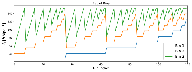
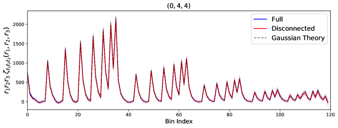
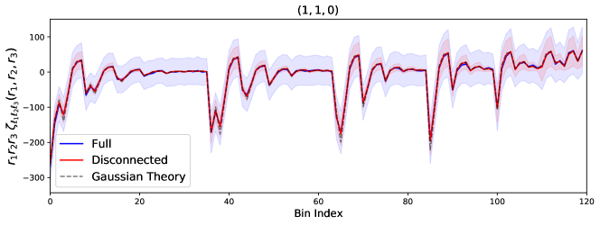
Figure 2: Full and disconnected 4PCF multiplets estimated from a suite of 1 000 lognormal mocks at $z=2$. The first panel shows the values of the linearly-averaged radial bin-centers, with the horizontal axis giving the index of the bins, collapsed into one dimension. Bins are ordered in increasing radius, and satisfy $r_{1}<r_{2}<r_{3}$. In the succeeding panels, we display the 4PCF of three representative multiplets (i.e. $\zeta_{\ell_{1}\ell_{2}\ell_{3}}$ for different choices of $\ell_{1},\ell_{2},\ell_{3}$), with the multiplets indicated by the title. Measurements using the full 4PCF estimator of §II are shown in solid blue lines, with those using the disconnected estimator of §III shown in solid red lines. In both cases the mean values are shown as lines with the shaded regions giving the $1\sigma$ errors. We further show the Gaussian theory model in dashed gray lines. The disconnected 4PCF closely matches the theory model, and furthermore, the connected 4PCF (equal to the difference between full and disconnected contributions) is small.

In Fig. 2, we compare the measured 4PCF multiplets from lognormal simulations with those of the analytic model (34), computed using the input power spectrum multipoles $P_{L}(k)$. We find good agreement between the disconnected measurements and the Gaussian theory model, affording us confidence that the disconnected 4PCF estimator works as expected. As noted in Appendix A, if the 2PCF is isotropic, only multiplets of the form $\{0,\ell,\ell\}$, $\{\ell,0,\ell\}$ or $\{\ell,\ell,0\}$ are non-zero; the clear non-zero $\zeta_{112}$ contributions shown in Fig. 2 highlight the importance of incorporating 2PCF anisotropies into the modelling. Furthermore, the connected contributions (equal to the difference between the full and disconnected estimator) are found to be very small. Again, this validates our procedure, since we are working at high redshift, whereupon the trispectrum contributions should be strongly suppressed. Motivated by these conclusions, we will henceforth display results only from the connected 4PCF estimator.

V Analysis Techniques

Given the estimators of §II & III and their verification in §IV, we are now in a position to consider how best to analyze the 4PCF of real surveys. Classically, cosmological data are analyzed by way of the $\chi^{2}$ statistic, defined as

$$\chi^{2}\equiv\left(\hat{\zeta}^{(\rm c)}-\zeta^{(\rm c)}_{\rm model}\right)^{T}\mathsf{C}^{-1}\left(\hat{\zeta}^{(\rm c)}-\zeta^{(\rm c)}_{\rm model}\right),$$ (36)

treating the connected 4PCF measurements as an $N_{\zeta}$-dimensional vector with covariance $\mathsf{C}$, implicitly summing over multiplets and bins. Here, our null hypothesis is that there is no connected 4PCF, hence $\zeta_{\rm model}^{(\rm c)}=\bm{0}$. It is common to use the sample covariance $\hat{\mathsf{S}}$ as a proxy for the true covariance:

$$\hat{\mathsf{S}}=\frac{1}{N_{\mathrm{mocks}}-1}\sum_{i=1}^{N_{\rm mocks}}\left(\zeta^{(\rm c)}_{i}-\bar{\zeta}^{(\rm c)}\right)\left(\zeta^{(\rm c)}_{i}-\bar{\zeta}^{(\rm c)}\right)^{T},$$ (37)

where $\{\zeta^{(\rm c)}_{i}\}$ are the 4PCF measurements from a suite of $N_{\rm mocks}$ mocks with mean $\bar{\zeta}^{(\rm c)}$. This gives the $\chi^{2}$ estimate

$$\hat{\chi}^{2}=\hat{\zeta}^{(\rm c),T}\hat{\mathsf{S}}^{-1}\hat{\zeta}^{(\rm c)}.$$ (38)

This approach bears a number of problems: (a) the sample covariance is invertible only if $N_{\rm mocks}>N_{\zeta}$, which is difficult to achieve given the high dimensionality of the 4PCF, (b) noise in the sample covariance matrix gives an additional source of noise in $\chi^{2}$, changing its probability distribution [58], and (c) an underlying assumption is that the 4PCF is Gaussian-distributed, which is questionable [e.g., 59, 60, 61, 62]. To ameliorate (a) and (b), one can replace $\hat{\mathsf{S}}$ with some theoretical covariance matrix (cf. §VI.3), which is straightforwardly invertible. However, with realistic survey geometries, the theoretical covariance is known to differ significantly from the measured covariance [51]. In this case, the expectation of (36) is not equal to $N_{\zeta}$ even under the null hypothesis of $\left\langle{\hat{\zeta}^{(\rm c)}}\right\rangle=\bm{0}$, thus it may lead to a spurious detection of non-Gaussianity. In [51] (and to an extent in [64, 65, 66]), it was suggested that altering the survey volume $V$ and number density $\bar{n}$ could partially absorb the effects of non-Gaussianity and window function non-uniformity; whilst this results in visually similar covariances, it can lead to spurious detections of non-Gaussianity, as discussed in Appendix B.

V.1 Data Compression

A convenient manner in which to deal with the curse of dimensionality is to compress the 4PCF data-vector $\zeta^{(\rm c)}$. Many compression schemes exist in the literature [e.g., 67, 68, 69, 38], all of which aim to reduce the dimension of the observable whilst retaining information contained within the Fisher matrix or log-likelihood. Since our goal is to simply make a measurement of non-Gaussianity, quantified by a $\chi^{2}$-like test under the null hypothesis, we will adopt a procedure similar to [31, 70], expanding the signal in a basis of approximate eigenmodes, then selecting those with maximal signal-to-noise. A key part of this is a theoretical covariance matrix; here, we use that of [51], which will be discussed further in §VI.3.

Explicitly, we first perform an eigendecomposition of the theory covariance matrix via $\mathsf{C}_{\rm theory}=\mathsf{U}\mathsf{D}\mathsf{U}^{T}$, where $\mathsf{U}$ is the unitary matrix of eigenvectors and $\mathsf{D}$ is a diagonal matrix of eigenvalues. Since the theory covariance is of full rank, we expect all eigenvalues to be non-zero. The 4PCF is then projected onto the eigenvectors via

$$v\equiv\mathsf{U}^{T}\zeta^{(\rm c)}.$$ (39)

Finally, we perform dimensionality reduction by restricting to the first $N_{\rm eig}$ eigenvectors, as ordered by signal-to-noise:

$$\left(\frac{S}{N}\right)_{i}=\frac{|\bar{v}_{i}|}{D_{i}},$$ (40)

where $\bar{v}$ is the mean 4PCF from a suite of realistic mocks (which we assume to be non-zero). Assuming $\mathsf{C}_{\rm theory}$ to be close to the true covariance, the compression scheme picks out the basis vectors that contribute most to the detection of non-zero $\chi^{2}$ in the data. Had our goal been to derive parameter constraints from the 4PCF, this decomposition would not be optimal, since the components contributing most to the signal-to-noise are not necessarily those with maximal information about the parameters of interest. In such a case, a Fisher- or likelihood-based compression scheme such as [67] or [69] would be preferred.

Following the compression, analysis proceeds in the low-dimensional subspace. In particular, we can define a new $\chi^{2}$ variable by compressing the mock 4PCF measurements and defining a sample covariance in the standard fashion (cf. 37):

$$\hat{\mathsf{S}}_{v}=\frac{1}{N_{\rm mocks}}\sum_{i=1}^{N_{\rm mocks}}\left(v_{i}-\bar{v}\right)\left(v_{i}-\bar{v}\right)^{T}\equiv\mathsf{U}^{T}\hat{\mathsf{S}}\mathsf{U},$$ (41)

assuming $\mathsf{U}$ to be of dimension $N_{\zeta}\times N_{\rm eig}$, i.e. dropping all but the highest signal-to-noise eigenmodes. If $N_{\rm mocks}>N_{\rm eig}$ this is invertible, meaning that a mock-based analysis is possible. The compressed $\chi^{2}$ is given by (cf. 38)

$$\hat{\chi}^{2}_{v}=\hat{v}^{T}\hat{\mathsf{S}}_{v}^{-1}\hat{v}\equiv\hat{\zeta}^{(\rm c),T}\mathsf{U}\left[\mathsf{U}^{T}\hat{\mathsf{S}}\mathsf{U}\right]^{-1}\mathsf{U}^{T}\hat{\zeta}^{(\rm c)}.$$ (42)

Since we apply the same compression to the data, the covariance, and the model, the compression cannot generate any spurious 4PCF signals, i.e. it is unbiased for any choice of projection matrix $\mathsf{U}$. In fact, the only effect of data compression is to lessen the significance of any detection. To see this, consider the case when $N_{\rm mocks}$ is large, such that $\hat{\mathsf{S}}\approx\mathsf{C}$. The signal-to-noise of some true 4PCF $\bar{\zeta}^{(\rm c)}$ is given by

$$\left(\frac{S}{N}\right)^{2}=\bar{\zeta}^{(\rm c)}\mathsf{C}^{-1}\bar{\zeta}^{(\rm c)},\qquad\left(\frac{S}{N}\right)^{2}_{v}=\bar{\zeta}^{(\rm c),T}\mathsf{U}\left[\mathsf{U}^{T}\mathsf{C}\mathsf{U}\right]^{-1}\mathsf{U}^{T}\bar{\zeta}^{(\rm c)},$$ (43)

pre- and post-compression respectively. Using the properties of projection matrices, we find that

$$\left(\frac{S}{N}\right)^{2}\geq\left(\frac{S}{N}\right)^{2}_{v}$$ (44)

for arbitrary $\bar{\zeta}^{(\rm c)}$, with equality only if $N_{\rm eig}=N_{\zeta}$, i.e. without projection. Thus, the compression can lead only to a reduced signal-to-noise; further, this is minimized by our choice of projection matrix $\mathsf{U}$. By the Eckart-Young theorem [71], our compression is optimal (in terms of signal-to-noise) if $\mathsf{C}_{\rm theory}=\mathsf{C}$. In practice, increasing $N_{\rm eig}$ might not lead to an increased detection significance, due to the broadening of the $\chi^{2}$ posterior when using a finite number of mocks, as we further discuss below.

V.2 Probability Distribution

If the data are Gaussian-distributed and the covariance is known precisely (i.e. in the limit $N_{\rm mocks}\to\infty$), the compressed $\chi^{2}$ statistic of (42) follows the $\chi^{2}$ distribution with $N_{\rm eig}$ degrees of freedom. In the case of a finite number of mocks, we must account for the effects of noise in the sample covariance, which changes the distribution of (42). A commonly-used approach is to rescale (42) by the Hartlap factor, i.e.

$$\hat{\chi}^{2}_{v}\to\frac{N_{\rm mocks}-N_{\rm eig}-2}{N_{\rm mocks}-1}\hat{\chi}^{2}_{v}\equiv\hat{H}^{2}_{v}$$ (45)

[72, 73], which debiases the inverse sample covariance. In this case, $\hat{H}^{2}_{p}$ is then analyzed using the $\chi^{2}$ distribution with $N_{\rm eig}$ degrees of freedom.

As shown in [58], this is not a consistent manner in which to treat noise in the sample covariance. Instead, the data follow the $t$-distribution, with the PDF

$$f_{T}(T^{2};n,p)=\frac{\Gamma\left([n+1]/2\right)}{\Gamma(p/2)\Gamma\left([n-p+1]/2\right)}\frac{n^{-p/2}(T^{2})^{p/2-1}}{(T^{2}/n+1)^{(n+1)/2}}$$ (46)

[58], denoting the sample statistic of (42) by $T^{2}$ and writing $n=N_{\rm mocks}-1$ and $p=N_{\rm eig}$ for Gamma function $\Gamma$. At finite $N_{\rm mocks}$, $f_{T}$ has a greater width than the $\chi^{2}$ distribution and will be used to avoid false signal detections.

V.3 Likelihood Non-Gaussianity

An underlying assumption in the above sections is that the likelihood for the 4PCF is Gaussian; i.e. that $\hat{\zeta}$ is a draw from some multivariate normal distribution with covariance $\mathsf{C}$. However, higher-order statistics such as the NPCFs are known to have increasingly non-Gaussian distributions as $N$ increases [e.g., 59, 60, 61, 62], thus performing a $\chi^{2}$ analysis (or a variant such as 46) may significantly over- (or under-)estimate the detection significance. In general, empirical determination of likelihood non-Gaussianity is difficult (though see [62] for an interesting approach) and beyond the scope of this work. Since the bulk of our analysis is performed on compressed statistics with $\mathcal{O}(100)$ elements, we expect the Central Limit Theorem to significantly reduce any non-Gaussianity present. A simple check of this reduction is to take a set of simulations and split them into two pieces, one of which is used to determine the sample mean and covariance, and the other of which is used as mock data. One may then compare the empirical distribution of $\hat{\chi}^{2}_{v}$ (including the sample mean) to the expected distribution (46). A visual comparison suggests that the degree of non-Gaussianity is not of particular importance; that said we encourage the reader to take the exact detection significances quoted below with a grain of salt, and hope to examine these effects in more detail in future work.

VI Practical Application

Below, we consider the practicalities of computing and analyzing the 4PCF from observational data, including discussion of the theoretical covariance matrix.

VI.1 Data and Simulations

Our dataset comprises galaxies from the twelfth data release (DR12) [74] of the Baryon Oscillation Spectroscopic Survey (BOSS), part of SDSS-III [75, 76]. In particular, we use the CMASS region, containing a total of 587 071 (216 041) galaxies in the redshift range $z_{\mathrm{min}}=0.43$ to $z_{\mathrm{max}}=0.7\}$ from the North (South) Galactic Cap (hereafter denoted ‘NGC’ and ‘SGC’). Here, we use both the galaxy data (converting angles and distances into Cartesian coordinates using our fiducial cosmology) and a set of unclustered randoms of $\sim$ $50\times$ greater number density. Galaxies are assigned weights as in [52]:

$$w_{\mathrm{tot}}=(w_{\mathrm{rf}}+w_{\mathrm{fc}}-1)w_{\mathrm{sys}}w_{\mathrm{fkp}}$$ (47)

where $w_{\mathrm{rf}}$, $w_{\mathrm{fc}}$ and $w_{\mathrm{sys}}$ correspond to redshift-failure, fiber-collision and systematic weights, with $w_{\mathrm{fkp}}=[1+n(z)P_{0}]^{-1}$ being the FKP weight [77] for background number density $n(z)$ and $P_{0}=10^{4}\,h^{-3}\mathrm{Mpc}^{3}$. The FKP weight ensures optimal spectrum extraction on small scales. Similar considerations apply for the random weights, except that the BOSS randoms do not contain any completeness or systematic weights.

To generate sample covariance matrices for our 4PCF statistic (required in §V), we use a suite of $1\,000$ MultiDark-Patchy (hereafter ‘Patchy’) simulations [79, 80], with the same survey geometry and radial selection function as the BOSS sample, both for the NGC and SGC regions. Weights are assigned via

$$w_{\mathrm{tot}}=w_{\mathrm{veto}}w_{\mathrm{fc}}w_{\mathrm{fkp}}$$ (48)

where $w_{\mathrm{veto}}$ is the veto flag (either zero or one), arising, from, for example, bright star masks. The Patchy simulations additionally have a separate random catalog.

VI.2 4PCF Computation

As in §IV, we compute the 4PCF multiplets, $\zeta_{\ell_{1}\ell_{2}\ell_{3}}^{abc}$, using the encore code [48]. As in §IV, we use $N_{r}=10$ radial bins per dimension with $r_{\mathrm{min}}=20\,h^{-1}\mathrm{Mpc}$, $r_{\mathrm{max}}=160\,h^{-1}\mathrm{Mpc}$. Given the additional restriction $r_{1}<r_{2}<r_{3}$, in order to avoid zero-separation bins, we have a total of 120 radial components per multiplet. To accurately capture the dominant signal contributions, we compute all $\{\ell_{1},\ell_{2},\ell_{3}\}$ multiplets up to $\ell_{\mathrm{max}}=5$, but use the $\ell=5$ elements only for edge correction. In total, we estimate $8\,280$ 4PCF components, of which $5\,040$ are used in the analysis of §VII. Whilst increasing the number of bins ensures that any fine features (such as BAO) are fully resolved, this incurs a significant computational penalty both in dimensionality of the output statistic (which is bounded from above by $N_{r}^{3}[\ell_{\mathrm{max}}+1]^{3}$) and in computation time (which scales as $N_{\rm g}N_{r}^{3}(\ell_{\mathrm{max}}+1)^{5}$ for $N_{\rm g}$ galaxies).

For computational ease, we split the random catalogs into 32 chunks, each containing $1.5\times$ more randoms than galaxies, and analyze each corresponding ‘data-minus-random’ catalog separately, using (11). Notably, we store the $a^{i}_{\ell m}(\bm{s})$ counts (10) from each ‘data-data’ particle pair after the first iteration to avoid unnecessary re-computation. All simulations are analyzed on a 16-core Intel processor (of various generations), embarrassingly parallelized using OpenMP. We simultaneously compute both the full 4PCF counts (13) and the two- and three-particle counts required to compute the disconnected piece (25) & (31), which are combined straightforwardly in post-processing using Python. In total, computation of the connected 4PCF requires $\sim$ $40$ ($6$) CPU-hours per NGC (SGC) simulation, or a total of $\sim$ $50$k CPU-hours for the complete set of data and 1 000 Patchy mocks. The inclusion of the disconnected component is found to increase the runtime by $\sim 20\%$. Whilst not insignificant, the runtime is comparable to the computational cost of the 2PCF analysis in [81].

VI.3 Analytic Covariance Matrices

To facilitate the data compression techniques discussed in §V.1, we require a smooth approximation to the connected 4PCF covariance matrix. For this purpose, we will use that derived in [51], under the assumptions of isotropy (i.e. no redshift-space distortions), Gaussianity (i.e. no contributions from NPCFs with $N>2$) and a uniform survey geometry. Whilst these assumptions lead to a covariance that does not precisely match the sample covariance of a realistic survey (as found in [51] for the MultiDark-Patchy simulations, and demonstrated here in Fig. 4), they do offer an analytically tractable theory. We recall that our compression scheme does not require the theoretical covariance to be unbiased; rather it should be smooth and have eigenvectors close to those of the true covariance.

Before projection onto the angular basis, the covariance matrix of the full 4PCF (including both connected and disconnected contributions) is defined by:

$$\mathrm{Cov}(\bm{r}_{1},\bm{r}_{2},\bm{r}_{3};\bm{r}_{1}^{\prime},\bm{r}_{2}^{\prime},\bm{r}_{3}^{\prime})=\left\langle{\hat{\zeta}(\bm{r}_{1},\bm{r}_{2},\bm{r}_{3})\hat{\zeta}^{*}(\bm{r}_{1}^{\prime},\bm{r}_{2}^{\prime},\bm{r}_{3}^{\prime})}\right\rangle-\left\langle{\hat{\zeta}(\bm{r}_{1},\bm{r}_{2},\bm{r}_{3})}\right\rangle\left\langle{\hat{\zeta}^{*}(\bm{r}_{1}^{\prime},\bm{r}_{2}^{\prime},\bm{r}_{3}^{\prime})}\right\rangle.$$ (49)

Inserting (6), this involves the expectation of eight density fields. As noted in [51], the Gaussian covariance contains two contributions: ‘fully coupled’ (including correlations only between density fields in different 4PCFs, e.g., between $\delta(\bm{s}+\bm{r}_{1})$ and $\delta(\bm{s}^{\prime}+\bm{r}_{1}^{\prime})$), and ‘partially coupled’ (including one correlation within each 4PCF, e.g., between $\delta(\bm{s}+\bm{r}_{1})$ and $\delta(\bm{s}+\bm{r}_{2})$). Respectively, these give the covariance contributions

$$\mathrm{Cov}^{(fc)}\left(\bm{r}_{1},\bm{r}_{2},\bm{r}_{3},\bm{r}_{1}^{\prime},\bm{r}_{2}^{\prime},\bm{r}_{3}^{\prime}\right) = \frac{1}{V}\int d\bm{s}\,\xi(\bm{s}+\bm{r}_{0}-\bm{r}_{0}^{\prime})\xi(\bm{s}+\bm{r}_{1}-\bm{r}_{1}^{\prime})\xi(\bm{s}+\bm{r}_{2}-\bm{r}_{2}^{\prime})\xi(\bm{s}+\bm{r}_{3}-\bm{r}_{3}^{\prime})+\text{23 perms.}$$

$$\mathrm{Cov}^{(pc)}\left(\bm{r}_{1},\bm{r}_{2},\bm{r}_{3},\bm{r}_{1}^{\prime},\bm{r}_{2}^{\prime},\bm{r}_{3}^{\prime}\right) = \xi(\bm{r}_{1}-\bm{r}_{0})\xi(\bm{r}_{1}^{\prime}-\bm{r}_{0}^{\prime})\,\frac{1}{V}\int d\bm{s}\,\xi(\bm{s}+\bm{r}_{2}-\bm{r}_{2}^{\prime})\xi(\bm{s}+\bm{r}_{3}-\bm{r}_{3}^{\prime})+\text{71 perms.},$$ (50)

via Wick’s theorem. To simplify the permutation structure of (VI.3), we have introduced dummy variables $\bm{r}_{0}$ and $\bm{r}_{0}^{\prime}$; these can be later set to zero. Here, we require the covariance of the connected 4PCF estimator (22), which requires only the ‘fully-coupled’ terms of (VI.3) [51]. All partially-coupled terms are cancelled by subtraction of the disconnected piece (22), which significantly reduces the estimator covariance. An explicit demonstration of this is given in Appendix C.

The above argument extends naturally to the 4PCF multiplets. In this case, the covariance becomes

$$\mathrm{Cov}_{\ell_{1}\ell_{2}\ell_{3};\,\ell_{1}^{\prime}\ell_{2}^{\prime}\ell_{3}^{\prime}}(r_{1},r_{2},r_{3};r_{1}^{\prime},r_{2}^{\prime},r_{3}^{\prime}) = \int\left[\prod_{i=1}^{3}d\hat{\bm{r}}_{i}\,d\hat{\bm{r}}^{\prime}_{i}\right]\,\mathrm{Cov}\left(\bm{r}_{1},\bm{r}_{2},\bm{r}_{3},\bm{r}_{1}^{\prime},\bm{r}_{2}^{\prime},\bm{r}_{3}^{\prime}\right)$$

$$\,\times\,\mathcal{P}_{\ell_{1}\ell_{2}\ell_{3}}^{*}(\hat{\bm{r}}_{1},\hat{\bm{r}}_{2},\hat{\bm{r}}_{3})\mathcal{P}_{\ell_{1}\ell_{2}\ell_{3}}^{*}(\hat{\bm{r}}_{1}^{\prime},\hat{\bm{r}}_{2}^{\prime},\hat{\bm{r}}_{3}^{\prime});$$

the simplified forms for this are given explicitly in [51]. It is straightforward to include radial binning in the covariance by replacing any spherical Bessel functions in (VI.3) with their bin-averaged equivalents as in (64). Both basis projection and radial binning are included in the covariances used in §VII.

To implement the Gaussian covariance, we require a model for the (survey-geometry-corrected) galaxy power spectrum. Here, we first compute the power spectrum multipoles, $P_{\ell}(k)$ (for $\ell\in\{0,2,4\}$), of the Patchy simulations using nbodykit [56], adopting a $k$-space binning of $k_{\mathrm{min}}=0.005h\,\mathrm{Mpc}^{-1}$, $k_{\mathrm{max}}=0.25h\,\mathrm{Mpc}^{-1}$ and $\Delta k=0.005h\,\mathrm{Mpc}^{-1}$. Since this work uses the CMASS sample, rather than the ‘z1’ and ‘z3’ split found in BOSS power spectrum analyses [e.g., 52, 82], we recompute the window function multipoles, $RR_{\ell}(r)$, by performing finely binned angular and radial pair-counts of the random particle catalog using corrfunc [83], downsampling the randoms by a factor of five for tractability. As in [84, 52], these facilitate comparison of the unwindowed power spectrum model and the window-convolved data. Data are fitted using a one-loop Effective Field Theory of Large Scale Structure model using the class-pt code [85] and the bias parametrization of [82]. This was recently shown to have exquisite accuracy on huge volume simulations [86], and we follow the treatment and bias parametrization of [82]. The unwindowed best-fit power spectrum is then used as an input to the analytic covariance. For simplicity, we compute only a single theory model using the NGC data, since the two hemispheres are found to have similar bias parameters [82]. To define the volume and shot-noise of each region we use the approach of [66, Appendix A] involving the random particle catalog, as described in [51].

VII Results

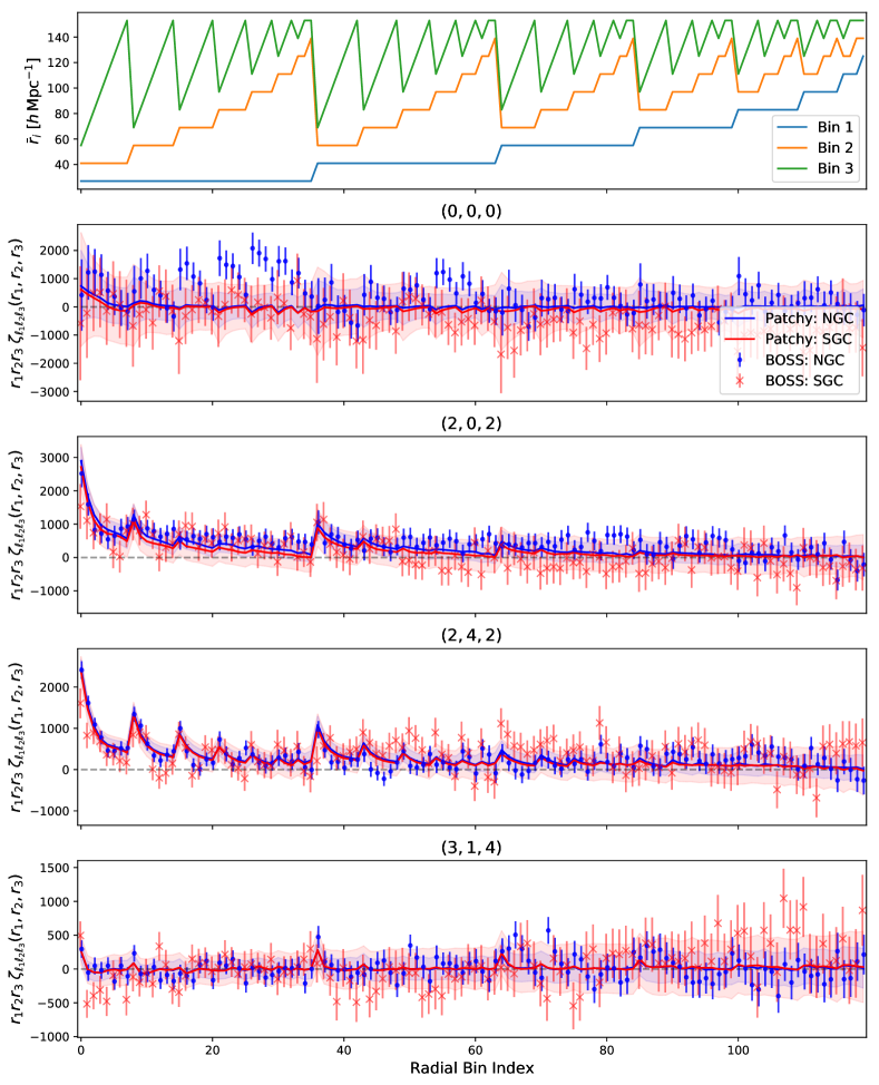
Figure 3: Connected 4PCF measurements from the BOSS CMASS dataset, alongside a suite of 1 000 Patchy mocks. Results from the NGC (SGC) region are shown in blue (red), with the lines and shaded regions showing the mean and $1\sigma$ deviations from Patchy respectively. As in Fig. 2, the first panel shows the radial bins corresponding to each one-dimensional bin index, and the lower panels give the results for a subset of the 42 measured multiplets, $\zeta_{\ell_{1}\ell_{2}\ell_{3}}$ (rescaled by $r_{1}r_{2}r_{3}$), with the values of $\ell_{1},\ell_{2},\ell_{3}$ given in the title. Though the measurements are both highly correlated and noisy, there is a clear non-zero signal observed, particularly in bins where the three side lengths are small. Any such detection is evidence of (gravitationally-induced) non-Gaussianity in the dataset.

In Fig. 3, we show a selection of the 42 connected 4PCF multiplets measured from the BOSS dataset and the Patchy simulations. Considering first Patchy, we find that, whilst the measurements are noisy, those from the mean-of-the-mocks show strong evidence for a non-zero connected 4PCF, i.e. for gravitational non-Gaussianity. This is enhanced on scales with small tetrahedron side lengths (i.e. small $\bar{r}_{i}$ in the figure); since structure forms first on small scales, this is as expected. Results from the NGC and SGC Patchy datasets are broadly consistent, though the latter has $\sim$ $2.5\times$ larger variance due to the smaller survey volume. Considering next the BOSS results, we find a similar story, i.e. a noisy dataset with generally increasing amplitudes on small scales. Overall, the observational dataset appears consistent with the distribution of Patchy mocks; unlike for the 2PCF and 3PCF [79], the Patchy mocks are not calibrated using the 4PCF data, thus the agreement in the 4PCF is not necessarily obvious a priori. Due to the high correlations between individual 4PCF measurements, it is difficult to assert a strong detection of non-Gaussianity from a visual inspection of the BOSS dataset; rather, we look to a statistical analysis, as described below.

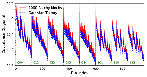
(a) Variance Comparison

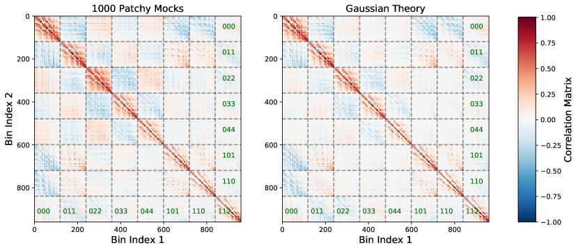
(b) Correlation Comparison

Figure 4: Comparison of sample and theoretical covariance matrices for the connected 4PCF used in this work. We show results only for the NGC region, with sample covariances computed from (37) using 1 000 Patchy mocks. The theoretical covariances are those of [51] and assume isotropy, Gaussianity and a periodic-box geometry. Fig. 4a shows the diagonal elements of the covariance, whilst Fig. 4b compares the correlation matrices, defined as the covariance normalized by its diagonal (i.e. $\mathsf{C}_{ij}/\sqrt{\mathsf{C}_{ii}\mathsf{C}_{jj}}$). Each submatrix refers to a different set of multiplets $\{\ell_{1},\ell_{2},\ell_{3}\}$, labelled in green, and within the submatrices, the elements are ordered in increasing radius as in Fig. 3. We show only the first 8 out of 42 multiplets for clarity. We note generally good agreement between the matrices, though some differences are evident on the diagonal. Since the theoretical covariance is only used as a tool to facilitate efficient data compression, such differences do not bias the analysis of this work.

In Fig. 4 we show the variance and correlation matrix of the connected 4PCF, measured from the 1 000 Patchy simulations using (37). As for the lower-point functions, the variance is a strongly declining function of scale (comparing with the bin-centers shown in Fig. 3); however, if one multiplies by $r_{1}r_{2}r_{3}$ (as in Fig. 3), it is roughly scale-independent. This reaffirms our conclusion that non-Gaussianity can be best probed on small scales (i.e. using tetrahedrons with at least one short side), where the signal is largest. From the correlation matrices (equal to the covariances normalized by their diagonal), we see strong off-diagonal contributions approaching unity for bins within the same $\{\ell_{1},\ell_{2},\ell_{3}\}$ multiplet. This is again visible in Fig. 3 in the coherent fluctuations between neighboring bins, and is a consequence of the high dimensionality of the 4PCF statistic. Significant (anti-)correlations are also seen between neighboring multiplets (i.e. those with $\ell$’s differing by at most one), which is a generic feature of our basis, and is similar to the structure found for the 3PCF in [14].

Additionally shown in Fig. 4 is a comparison between the Patchy sample covariance and the theoretical covariance discussed in §VI.3. From the diagonal elements, we see that the variance is fairly well reproduced by the Gaussian model, though the ratio of sample to theory covariance is roughly $1.7\pm 0.6$, showing an overall underprediction from the theory. More troublingly, this ratio is observed to vary with $\ell$; for example, results from the $\{1,1,0\}$ multiplet match the sample covariance well, but those from the $\{0,4,4\}$ multiplet are a clear underprediction. On the other hand, the correlation plots indicate that the matrix structure is well reproduced, including the non-trivial correlations within multiplets and between them. In [51], it was shown that the 4PCF covariance was a good model for simulations with periodic-box geometries; it is therefore likely that the discrepancies arise due to the impact of the non-uniform survey geometry. Such effects are known to be of importance in the covariances of lower-order statistics [e.g., 87, 66, 64, 65, 88], thus this is unsurprising. If the theoretical covariances were being used directly in the analysis this would be a cause for concern (as shown in Appendix B), but is not in our context, since the theory covariance is used only to define the compression vectors (§V.1).

Figure 5: PDFs of the test statistics discussed in §V, showing the significance of a detection of non-zero 4PCF in the BOSS CMASS dataset as a function of the number of basis vectors in the compression scheme, $N_{\rm eig}$. In orange and blue we show the $H^{2}$ and $T^{2}$ statistics respectively, both of which are related to the $\chi^{2}$ statistic, but differently account for the finite number of mocks. The $H^{2}$ statistic follows a $\chi^{2}$-distribution, which will show a reduced width as $N_{\rm eig}$ approaches $N_{\rm mocks}$. Sample covariances are computed by jackknifing the 1 000 Patchy mocks (using each subset of 999 mocks to define a sample covariance), and results are shown for four choices of compressed data-vector size, with the BOSS data shown as vertical dashed lines. The sample statistics of the NGC and SGC regions are summed, giving a resulting distribution that can be evaluated via a convolution (as discussed in the main text). In each case, we report a strong detection of non-Gaussianity, at the level equivalent to a Gaussian significance of $8.1\sigma,8.2\sigma$ and $8.1\sigma$ for $N_{\rm eig}=10$, $50$, and $100$ respectively, using the $T^{2}$ statistic.

Given the connected 4PCF measurements and covariances, we may proceed to assess the significance of a detection of non-Gaussianity. As in §V.1, we first compress the data by projecting it onto a basis of eigenmodes of the theory covariance. Here, we perform the compression for the NGC and SGC regions separately (assuming them to be uncorrelated), using $N_{\rm eig}=10,50,$ or $100$. The test statistics $H^{2}$ (the Hartlap-rescaled $\chi^{2}$ of 45) and $T^{2}$ (from 42) are computed both for the BOSS data and the Patchy mocks (obtaining the relevant covariance matrices via jackknifing in the latter case), then compared to the theory distributions. To combine the two data chunks, we simply add the $H^{2}$ or $T^{2}$ sample statistics, such that their expected distributions (under the null hypothesis) become the convolution of two $\chi^{2}$ distributions or of two copies of (46) (both with $N_{\rm eig}$ degrees of freedom). These are easily evaluated using Fast Fourier Transforms of the single-sample PDFs. For small $N_{\rm eig}$, we expect both likelihoods to yield similar results, though the less-conventional $T^{2}$ statistic is the more appropriate choice as $N_{\rm eig}$ approaches $N_{\rm mocks}$ [58].

Fig. 5 shows the test statistics obtained from the Patchy and BOSS data compared against the distribution expected under the null hypothesis of zero connected 4PCF. The conclusion is readily apparent; we report a strong detection of non-Gaussianity in the 4PCF of BOSS. By comparing the BOSS $T^{2}$ statistic to the CDF of the null distribution, we find a probability-to-exceed of $\sim$ $10^{-15}$; this corresponds to a Gaussian detection significance of $\sim$ $8\sigma$. As $N_{\rm eig}$ increases, the detection significances remain consistent; this indicates that our compression scheme has captured the majority of the signal-to-noise, and that we are not yet limited by the number of mocks. Extending to $N_{\rm eig}=250$, the detection significance reduces to $\sim$ $7\sigma$, due to the limited number of mocks. We further note that the BOSS and Patchy results are highly consistent, as observed in Fig. 3. The results are broadly consistent using the Hartlap-rescaled statistic $H^{2}$ and its $\chi^{2}$-distribution, though the detection significance increases to $\sim$ $8.5\sigma$ with $N_{\rm eig}=250$, most likely due to the artificially narrow theory distribution. We caution however that non-Gaussianity of the 4PCF likelihood will modify the exact detection significances somewhat (cf. §V.3).

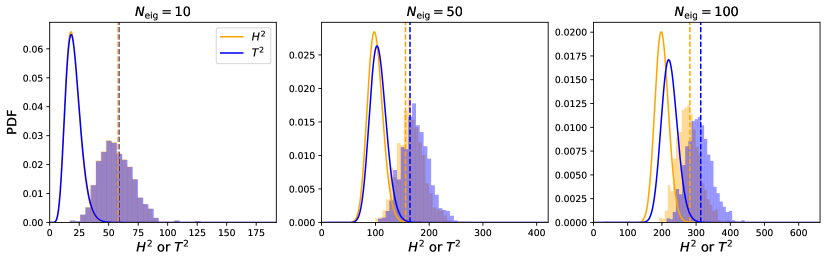
Figure 6: As Fig. 5, but enforcing a minimum separation of $\Delta r=14\,h^{-1}\mathrm{Mpc}$ between any two galaxies forming the 4PCF tetrahedra. In this case, we find the detection strength is equivalent to a Gaussian significance of $4.7\sigma$, $4.0\sigma$ and $4.0\sigma$ for $N_{\rm eig}=10,50$, and $100$ respectively. As expected, this significance is less than that of Fig. 5, since the non-Gaussian signature is found primarily on short-scales. However, this result provides a practical sense of the useful 4PCF signal strength, since the modes expected to be most difficult to model have been removed.

As observed in Fig. 3, most of the signal-to-noise in the connected 4PCF occurs on small scales, where non-Gaussianity is largest. Whilst our analysis has restricted to $r_{\rm min}=20\,h^{-1}\mathrm{Mpc}$, this does not in fact enforce a minimum separation on all points in the 4PCF tetrahedron, just the distance of the secondary galaxies from some primary vertex. As an example, a 4PCF bin with $r_{1}$, $r_{2}$ and $r_{3}$ legs in the ranges $[20,34)\,h^{-1}\mathrm{Mpc}$, $[34,48)\,h^{-1}\mathrm{Mpc}$ and $[48,62)\,h^{-1}\mathrm{Mpc}$ (corresponding to the first bin in Fig. 3), can have arbitrarily small (though non-zero) values of $|\bm{r}_{1}-\bm{r}_{2}|$ and $|\bm{r}_{2}-\bm{r}_{3}|$. Whilst not a problem for the detection of the 4PCF, such modes are challenging to model since any perturbative description necessarily breaks down beyond the non-linear scale and there will be significant effects from baryonic physics not included in simulations. To this end, we consider restricting to bins with centers separated by greater than $\Delta r=14\,h^{-1}\mathrm{Mpc}$; this enforces a minimum separation of $\Delta r$ between each galaxy in the 4PCF tetrahedron, thus avoiding the most difficult-to-model modes. It additionally reduces the dimensionality by a factor of roughly two. The corresponding detection PDFs are shown in Fig. 6, and are heuristically similar to those of Fig. 5. Here, we find a probability-to-exceed of $\sim$ $10^{-5}$, equivalent to a Gaussian significance of $\sim$ $4.7\sigma$ for $N_{\rm eig}=10$. Whilst this significance is noticeably decreased from that of Fig. 3, it is still a clear detection, implying that a non-zero 4PCF can still be detected in the BOSS dataset when restricting to scales outside the non-linear regime.

VIII Summary and Conclusions

To maximize the information gain from future spectroscopic surveys, it is vital to harness statistics that extract maximal information from the galaxy density field. Whilst analyses have historically focused around the 2PCF or power spectrum, there has been a recent effort to extract information from the higher-point functions, in particular the 3PCF or bispectrum [17, 19, 20, 39]. In this work, we present a practical method for measuring the next-order statistic, the 4PCF, and quantify its signal-to-noise in the BOSS dataset. In particular, we extend the NPCF algorithms of [48, 49] to measure the connected 4PCF by removing the Gaussian piece (which is degenerate with the 2PCF) at the estimator level. This is unlike previous works, and ensures that our measurement is specifically one of non-Gaussianity, rather than a recapitulation of known physics. The estimator is fast (scaling quadratically with the galaxy number density), corrected for the non-uniform survey geometry, and implemented in the public encore code. We verify its performance on a suite of lognormal simulations at high redshift, before applying it to the BOSS dataset and Patchy simulations. Analysis of the higher-point functions is hampered by their high dimension; here, we implement a signal-to-noise-based compression scheme (originally proposed in [31]), which allows us to project the 4PCF into a set of $\sim 50$ numbers with minimal impact on the detection significance. Performing a classical $\chi^{2}$-like analysis in the compressed subspace leads to an $8.1\sigma$ detection of the non-Gaussian 4PCF, or $4.7\sigma$ if we restrict to galaxy quadruplets with separations outside the highly non-linear regime.

Based on this work, a number of avenues present themselves for future study:

• Theory Model: To extract information from the 4PCF, we require a physical model for its dependence on cosmological and galaxy formation parameters. Whilst this is not trivial to compute, it is tractable, at least at tree level. Simulation-based approaches, such as emulators [e.g., 89], also provide an interesting prospect for obtaining theory predictions in difficult-to-model regimes.

• Fisher Forecasting: In the absence of a theory model, one can test the information content of the 4PCF with simulation-based Fisher forecasts. This requires a large number of simulations of varying cosmological and hydrodynamic parameters [e.g., 10], which may be analyzed using a fast algorithm such as encore.

• Odd-Parity 4PCF: The present work has considered only 4PCF multiplets with even $\ell_{1}+\ell_{2}+\ell_{3}$, i.e. the contribution invariant under parity transformations. Complementary to this is the set of multiplets with odd $\ell_{1}+\ell_{2}+\ell_{3}$, which can be measured in a similar fashion, and probes parity-violating physics. This will be discussed in [47].

• Anisotropic 4PCF: Due to redshift-space distortions, the density field is statistically anisotropic, with azimuthal symmetry about the line of sight. As such, the full 4PCF contains both an isotropic contribution (discussed in this work) and an anisotropic component. The latter can be probed in a similar manner to this work (using the estimators derived in [49]), and will allow all the 4PCF information to be captured.

• 4PCF Likelihood: A major assumption in this work is that the 4PCF is drawn from some multivariate Gaussian distribution. As shown in a number of works [e.g., 60, 62, 61], this assumption is questionable and should be examined further, particularly if one wishes to use the 4PCF to derive constraints on cosmological parameters.

• Observational Systematics: Since the present work has focused on the detectability of the non-Gaussian 4PCF signal, we have assumed that the standard galaxy weighting scheme (§VI) can sufficiently account for systematic effects in the data. To derive parameter constraints from our signal, a more careful treatment of such effects, in particular those of fiber collisions, is likely needed.

Given the significance with which we can detect the 4PCF in current datasets, it is worth considering prospects for future surveys. Whilst the cosmic volume mapped will grow dramatically with efforts such as DESI and Euclid, the majority of the galaxy observations will take place at higher redshifts, where the relative importance of the 4PCF will be severely diminished. In particular, the squared signal-to-noise of a 4PCF detection scales with redshift approximately as $D^{4}(z)$ for linear growth rate $D(z)$, and linearly with volume. Using the effective volume and redshift parameters from [4, Table 2.3] and [9, Table 1], a back-of-the-envelope calculation suggests that the overall 4PCF squared signal-to-noise will increase by a factor of $\sim$ $60\%$ and $\sim$ $100\%$ for DESI and Euclid respectively, assuming the tracers to be similar. This is significantly below that which one might expect from pure volume-rescaling arguments, and is caused by the strong redshift dependence. That said, the detection is still likely to be strong, and consequently one may expect the 4PCF to become a useful probe of physical parameters, both those pertaining to $\Lambda$CDM and to more exotic phenomena such as primordial non-Gaussianity and modified gravity.

Appendix A Gaussian Theory Model

Below, we derive the expected form of the 4PCF in the Gaussian (but non-linear) regime, i.e. the disconnected term, as discussed in §IV. Before projection, the Gaussian 4PCF is given by a set of Wick contractions of pairs of density fields:

$$\zeta^{\mathrm{G}}(\bm{r}_{1},\bm{r}_{2},\bm{r}_{3}) = \left\langle{\delta(\bm{s})\delta(\bm{s}+\bm{r}_{1})\delta(\bm{s}+\bm{r}_{2})\delta(\bm{s}+\bm{r}_{3})}\right\rangle=\xi(\bm{r}_{1})\xi(\bm{r}_{2}-\bm{r}_{3})+\text{2 perms.}$$

$$= \xi(\bm{r}_{1})\int_{\bm{k}}P(\bm{k})e^{i\bm{k}\cdot(\bm{r}_{2}-\bm{r}_{3})}+\text{2 perms.},$$

writing the 2PCF in terms of the power spectrum in the second line. Accounting for RSD, $\xi(\bm{r})$ and $P(\bm{k})$ may be expanded as Legendre series around the (assumed fixed) line-of-sight (LoS) $\hat{\bm{n}}$:

$$\xi(\bm{r})=\sum_{L}\xi_{L}(r)L_{L}(\hat{\bm{r}}\cdot\hat{\bm{n}}),\quad P(\bm{k})=\sum_{L}P_{L}(k)L_{L}(\hat{\bm{k}}\cdot\hat{\bm{n}}),$$ (53)

where $L_{L}(\mu)$ is a Legendre polynomial of order $L$, which is even if the overdensity field conserves parity. In the simplest instance of Kaiser linear theory [90], only moments with $L\in\{0,2,4\}$ are non-zero. Inserting (53) into (A) gives

$$\zeta^{\rm G}(\bm{r}_{1},\bm{r}_{2},\bm{r}_{3}) = \sum_{LL^{\prime}}\xi_{L}(r_{1})\int_{\bm{k}}P_{L^{\prime}}(k)e^{i\bm{k}\cdot(\bm{r}_{2}-\bm{r}_{3})}\int\frac{d\hat{\bm{n}}}{4\pi}L_{L}(\hat{\bm{r}}_{1}\cdot\hat{\bm{n}})L_{L^{\prime}}(\hat{\bm{k}}\cdot\hat{\bm{n}})+\text{2 perms.}$$

$$= \sum_{L}\frac{1}{2L+1}\,\xi_{L}(r_{1})\int_{\bm{k}}P_{L}(k)e^{i\bm{k}\cdot(\bm{r}_{2}-\bm{r}_{3})}L_{L}(\hat{\bm{r}}_{1}\cdot\hat{\bm{k}}),$$

where we have additionally inserted an angular integral over the LoS, justified since we consider only the isotropic 4PCF, which cannot depend on $\hat{\bm{n}}$. In the final line, we perform the $\hat{\bm{n}}$ integral via Legendre polynomial orthogonality [53, §14.7.6]. Expanding the exponentials $e^{i\bm{k}\cdot\bm{r}_{2}}$ and $e^{-i\bm{k}\cdot\bm{r}_{3}}$ via the Rayleigh plane wave identity [91, Eq., 16.63] gives

$$\int\frac{d\hat{\bm{n}}}{4\pi}\,\xi(\bm{r}_{1})\xi(\bm{r}_{2}-\bm{r}_{3}) = \sum_{L,\ell_{1},\ell_{2}}\frac{(4\pi)^{3}}{(2L+1)^{2}}\,i^{\ell_{1}-\ell_{2}}\xi_{L}(r_{1})\int_{\bm{k}}P_{L}(k)j_{\ell_{1}}(kr_{2})j_{\ell_{2}}(kr_{3})$$

$$\,\times\,Y_{L}^{M}(\hat{\bm{k}})Y_{\ell_{1}}^{m_{1}}(\hat{\bm{k}})Y_{\ell_{2}}^{m_{2}}(\hat{\bm{k}})Y_{L}^{M*}(\hat{\bm{r}}_{1})Y_{\ell_{1}}^{m_{1}*}(\hat{\bm{r}}_{2})Y_{\ell_{2}}^{m_{2}*}(\hat{\bm{r}}_{3}),$$

additionally rewriting the Legendre polynomial in terms of spherical harmonics [53, §14.30.9] and introducing spherical Bessel functions $j_{L}(x)$. The angular integral over $\hat{\bm{k}}$ yields a Gaunt integral [53, §34.3.22]; writing this explicitly in terms of 3-$j$ symbols gives

$$\int\frac{d\hat{\bm{n}}}{4\pi}\,\xi(\bm{r}_{1})\xi(\bm{r}_{2}-\bm{r}_{3}) = \sum_{L\ell_{1}\ell_{2}}\left[\frac{(4\pi)^{3}(2\ell_{1}+1)(2\ell_{2}+1)}{(2L+1)^{3}}\right]^{1/2}\begin{pmatrix}{L}&{\ell_{1}}&{\ell_{2}}\\ 0&0&0\end{pmatrix}i^{\ell_{1}-\ell_{2}}\xi_{L}(r_{1})$$

$$\,\times\,\int\frac{k^{2}dk}{2\pi^{2}}P_{L}(k)j_{\ell_{1}}(kr_{2})j_{\ell_{2}}(kr_{3})\sum_{Mm_{1}m_{2}}\begin{pmatrix}{L}&{\ell_{1}}&{\ell_{2}}\\ {M}&{m_{1}}&{m_{2}}\end{pmatrix}Y_{L}^{M*}(\hat{\bm{r}}_{1})Y_{\ell_{1}}^{m_{1}*}(\hat{\bm{r}}_{2})Y_{\ell_{2}}^{m_{2}*}(\hat{\bm{r}}_{3}).$$

We recognize the sum over three $m$ indices as the basis function $\mathcal{P}_{L\ell_{1}\ell_{2}}(\hat{\bm{r}}_{1},\hat{\bm{r}}_{2},\hat{\bm{r}}_{3})$ in (3) (assuming even $L+\ell_{1}+\ell_{2}$, such that $\mathcal{P}_{\ell_{1}\ell_{2}\ell_{3}}^{*}=\mathcal{P}_{\ell_{1}\ell_{2}\ell_{3}}$). By orthogonality, we can read off the multipole coefficients as

$$\zeta^{\mathrm{G}}_{L\ell_{1}\ell_{2}}(r_{1},r_{2},r_{3}) = i^{\ell_{1}-\ell_{2}}\left[\frac{(4\pi)^{3}(2\ell_{1}+1)(2\ell_{2}+1)}{(2L+1)^{3}}\right]^{1/2}\begin{pmatrix}{L}&{\ell_{1}}&{\ell_{2}}\\ 0&0&0\end{pmatrix}\xi_{L}(r_{1})\int\frac{k^{2}dk}{2\pi^{2}}P_{L}(k)j_{\ell_{1}}(kr_{2})j_{\ell_{2}}(kr_{3}),$$ (57)

with analogous results found for the other two permutations. This has support for all multiplets in which the triangle conditions on $\{L,\ell_{1},\ell_{2}\}$ are satisfied.

Defining

$$f^{L}_{\ell\ell^{\prime}}(r,r^{\prime})=\int\frac{k^{2}dk}{2\pi^{2}}P_{L}(k)j_{\ell}(kr)j_{\ell^{\prime}}(kr^{\prime}),$$ (58)

with the special case $f^{L}_{\ell 0}(r,0)=i^{-\ell}\xi_{\ell}(r)$, (57) can be written succinctly as

$$\zeta^{\mathrm{G}}_{\ell_{1}\ell_{2}\ell_{3}}(r_{1},r_{2},r_{3}) = \left[\frac{(4\pi)^{3}(2\ell_{2}+1)(2\ell_{3}+1)}{(2\ell_{1}+1)^{3}}\right]\begin{pmatrix}{\ell_{1}}&{\ell_{2}}&{\ell_{3}}\\ 0&0&0\end{pmatrix}i^{\ell_{2}-\ell_{3}}\xi_{\ell_{1}}(r_{1})f^{\ell_{1}}_{\ell_{2}\ell_{3}}(r_{2},r_{3})+\text{2 perms.}$$ (59)

An interesting case is the limit of zero RSD, in which case $\xi_{\ell}$ and $P_{\ell}$ are zero for $\ell>0$. Following simplification, this yields only three non-zero multiplets:

$$\zeta_{0\ell\ell}^{\mathrm{G,no\,RSD}}(r_{1},r_{2},r_{3}) = (4\pi)^{3/2}(-1)^{\ell}\sqrt{2\ell+1}\xi_{0}(r_{1})f^{0}_{\ell\ell}(r_{2},r_{3}),$$ (60)

$$\zeta_{\ell 0\ell}^{\mathrm{G,no\,RSD}}(r_{1},r_{2},r_{3}) = (4\pi)^{3/2}(-1)^{\ell}\sqrt{2\ell+1}\xi_{0}(r_{2})f^{0}_{\ell\ell}(r_{1},r_{3}),$$

$$\zeta_{\ell\ell 0}^{\mathrm{G,no\,RSD}}(r_{1},r_{2},r_{3}) = (4\pi)^{3/2}(-1)^{\ell}\sqrt{2\ell+1}\xi_{0}(r_{3})f^{0}_{\ell\ell}(r_{1},r_{2}).$$

A detection of non-zero 4PCF in any multiplet not of this form is thus evidence for RSD effects (in the disconnected piece) or non-Gaussianity (in the connected piece).

Finally, we consider radial binning. As in §II, the 4PCF algorithm natively measures the correlators averaged across bins of finite width, thus the same averaging must be performed for the theory model. Given a bin triplet $\{a,b,c\}$, the binned theory is defined by

$$\zeta^{abc}_{\ell_{1}\ell_{2}\ell_{3}}=\frac{(4\pi)^{3}}{v_{a}v_{b}v_{c}}\int r_{1}^{2}dr_{1}\,\Theta^{a}(r_{1})\int r_{2}^{2}dr_{2}\,\Theta^{b}(r_{2})\int r_{3}^{2}dr_{3}\,\Theta^{c}(r_{3})\,\zeta_{\ell_{1}\ell_{2}\ell_{3}}(r_{1},r_{2},r_{3}),$$ (61)

where $v_{u}=4\pi\int r^{2}dr\,\Theta^{u}(r)$. In the above model, binning can be simply realized by replacing $\xi_{\ell}$ and $f_{\ell_{1}\ell_{2}}^{L}$ by their binned equivalents, i.e.

$$\zeta^{\mathrm{G},abc}_{\ell_{1}\ell_{2}\ell_{3}} = (4\pi)^{3/2}\sqrt{(2\ell_{1}+1)(2\ell_{2}+1)(2\ell_{3}+1)}\begin{pmatrix}{\ell_{1}}&{\ell_{2}}&{\ell_{3}}\\ 0&0&0\end{pmatrix}$$

$$\,\times\,\left\{\frac{i^{\ell_{2}-\ell_{3}}}{(2\ell_{1}+1)^{2}}\,\xi^{a}_{\ell_{1}}f^{\ell_{1},bc}_{\ell_{2}\ell_{3}}+\frac{i^{\ell_{1}-\ell_{3}}}{(2\ell_{2}+1)^{2}}\,\xi^{b}_{\ell_{2}}f^{\ell_{2},ac}_{\ell_{1}\ell_{3}}+\frac{i^{\ell_{1}-\ell_{2}}}{(2\ell_{3}+1)^{2}}\,\xi_{\ell_{3}}^{c}(r_{3})f^{\ell_{3},ab}_{\ell_{1}\ell_{2}}\right\},$$

where

$$\xi_{\ell}^{u}=i^{\ell}\int\frac{k^{2}dk}{2\pi^{2}}P_{\ell}(k)j_{\ell}^{u}(k),\qquad f_{\ell\ell^{\prime}}^{L,uv}=\int\frac{k^{2}dk}{2\pi^{2}}P_{L}(k)j_{\ell}^{u}(k)j_{\ell^{\prime}}^{v}(k).$$ (63)

These use the bin-averaged spherical Bessel functions, defined by

$$j_{\ell}^{u}(k)=\frac{4\pi}{v_{u}}\int r^{2}dr\,j_{\ell}(kr)\Theta^{u}(r).$$ (64)

These are in fact analytic, and their general form can be expressed in terms of generalized hypergeometric functions as in [Appendix A 92]. For integer $\ell$, they are simple sums of trigonometric functions and the Sine integral, and easily evaluated using e.g.,, Mathematica. Performing such computations analytically allows for the theory model to be evaluated quickly and at high precision.

Appendix B Analysis Using a Fitted Theory Covariance Matrix

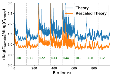
Figure 7: Comparison between the variances of the Patchy mocks and those obtained from the theoretical covariance model discussed in §VI.3. We present results both before and after fitting for the volume $V_{\rm eff}$ and shot-noise $\bar{n}_{\rm eff}$ by comparing the theoretical and sample covariances. Results are shown only for the first 8 of 42 multiplets, as in Fig. 4, again restricting to the NGC data chunk. The inclusion of fitting parameters leads to better agreement between theory and simulations, though not perfect, as evidenced by the underpredictions at small radii.

As demonstrated in Fig. 4, the Gaussian covariance derived in [51] is not in perfect agreement with the sample covariance from the Patchy mocks, particularly when the variance is considered. As advocated for in [51], one way to ameliorate this is to adjust the effective survey volume $V$ and shot-noise parameter $1/\bar{n}$, which can, to some extent, mimic the effects of non-uniform geometry and non-Gaussianity [cf., 64, 93, 65]. Here, we implement this approach, fitting for $V$ and $1/\bar{n}$ by comparing the theoretical and sample covariances using the Kullback-Leibler divergence as in [64], which accounts for the expected (Wishart) distribution of the mock-based covariance. For the NGC data chunk, minimization leads to the best-fit parameters $\{V_{\rm eff}=1.57h^{-3}\mathrm{Gpc}^{3},\bar{n}^{-1}_{\rm eff}=4.2\times 10^{3}\,h^{3}\mathrm{Mpc}^{-3}\}$, which differ significantly from the fiducial values $\{V=1.9h^{-3}\mathrm{Gpc}^{3},\bar{n}^{-1}=3.0\times 10^{3}\,h^{3}\mathrm{Mpc}^{-3}\}$. Comparison of the sample and theoretical variances, both before and after parameter fitting, are shown in Fig. 7. Noticeably, we find much improved agreement between Patchy and the theory model after the rescaling, implying that the free parameters have been able to account for some of the survey geometry and non-Gaussian effects. That said, there remain some systematic offsets in the rescaled theory covariance, particularly in bins corresponding to small radii.

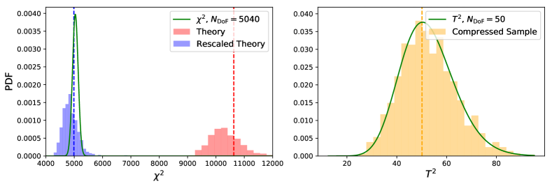
Figure 8: Distributions of the $\chi^{2}$ (left) and compressed $T^{2}$ (right) statistics from a set of mock 4PCFs with the mean subtracted. As before, the vertical lines give the corresponding results for BOSS. In the left panel, we show the $\chi^{2}$ statistic, computed using the theory covariance of §V.1 (red), optionally with fitted $V$ and $\bar{n}$ parameters (blue, cf. Fig. 7). Since the signal has been removed from the data, we should see agreement between the expected distribution (green) and the empirical histograms (blue and red) if the theoretical covariances are accurate; this is clearly not the case, both before and after fitting. In the right panel, we perform an analysis in the compressed subspace using $N_{\rm eig}=50$ basis vectors (cf. §V.1), plotting the $T^{2}$ statistic of (42) and the expected distribution of (46). In this case, we do not find any evidence for bias, as expected.

To test the rescaled covariance matrix more rigorously, we consider a scenario in which the expected 4PCF signal is zero, easily obtained by taking the connected 4PCF results from Patchy and subtracting the mean. This is of use since the distribution is known; if the theoretical covariances match the true underlying covariance (and the underlying likelihood is Gaussian), then the $\chi^{2}$ statistic

$$\left.\chi^{2}\right|_{\rm theory}=\tilde{\zeta}^{T}\mathsf{C}^{-1}_{\rm theory}\tilde{\zeta}$$ (65)

of the mean-subtracted data $\tilde{\zeta}$ will be distributed according to a $\chi^{2}$ distribution with $N_{\zeta}=5\,040$ degrees of freedom. In the left panel of Fig. 8, we plot the empirical $\chi^{2}$ distributions obtained from the $1\,000$ Patchy NGC simulations using both the fiducial and fitted theoretical covariance matrices, alongside the expected distribution. The fiducial (unrescaled) covariance leads to an empirical distribution which is highly inconsistent with that of the theory; a naïve analysis using this data would obtain $\chi^{2}/N_{\zeta}\approx 2$ and conclude a strong detection of non-Gaussianity, even though none was present in the data. When using the fitted covariance matrix, the result is far more reasonable (as expected, since one has effectively minimized the expectation of $|\chi^{2}-N_{\zeta}|$); however, the empirical and sample distributions are still not in agreement. In particular, the shape of the distribution is incorrect, and, for many data realizations, one would conclude that there was less non-Gaussianity present than in the null-hypothesis, which is nonsensical.

In the right panel of Fig. 8, we give the corresponding results for the mean-subtracted 4PCFs analyzed in the compressed subspace of §V.1 using $N_{\rm eig}=50$ and a sample covariance computed from 1 000 Patchy mocks. As discussed previously compression cannot lead to a spurious signal detection (assuming the 4PCF to be Gaussian distributed); this is borne out in practice, since the empirical distribution of $T^{2}$ is well modelled by its theory distribution (46). The excellent agreement also indicates that the non-Gaussianity in the 4PCF likelihood is not of significant importance here. Our main conclusion is the following: if one wishes to compute the 4PCF detection significance, it is dangerous to use the theoretical covariances directly in $\chi^{2}$, since this can give significant mis-detections of the signal even when none is present. Working in the compressed subspace avoids such concerns, even though it may lead to a slight loss of signal-to-noise if the theory covariance (used to define the basis vectors) is far from the truth.

Appendix C Connected 4PCF Covariance

In §VI.3, it was noted that the covariance matrix of the connected 4PCF contains only fully-coupled contributions (VI.3). Here, we provide an explicit demonstration of this, as well as a visual comparison of the full and connected 4PCF covariance matrices using lognormal simulations.

Firstly, consider the connected estimator in the form

$$\hat{\zeta}^{(\rm c)}(\bm{r}_{1},\bm{r}_{2},\bm{r}_{3}) = \frac{1}{V}\int d\bm{s}\,\delta(\bm{s}+\bm{r}_{0})\delta(\bm{s}+\bm{r}_{1})\delta(\bm{s}+\bm{r}_{2})\delta(\bm{s}+\bm{r}_{3})$$

$$\,-\,\left[\frac{1}{V}\int d\bm{s}\,\delta(\bm{s}+\bm{r}_{0})\delta(\bm{s}+\bm{r}_{1})\,\frac{1}{V}\int d\bm{s}^{\prime}\,\delta(\bm{s}^{\prime}+\bm{r}_{2})\delta(\bm{s}^{\prime}+\bm{r}_{3})+\text{2 perms.}\right]$$

again introducing the dummy variable $\bm{r}_{0}=\bm{0}$ for keeping track of the permutations. Computing the covariance of (C) and applying statistical homogeneity will give terms proportional to $V^{-\alpha}$ where $\alpha\in\{1,2,3\}$. Assuming the survey size to be much larger than the typical correlation length $r_{c}\approx 100\,h^{-1}\mathrm{Mpc}$, we may drop any terms with $\alpha>1$, since these are suppressed by powers of $r_{c}^{3}/V\ll 1$. As an example, consider the term arising from the expectation of two disconnected 4PCFs;

$$\left\langle{\zeta^{(\rm disc)}(\bm{r}_{1},\bm{r}_{2},\bm{r}_{3})\zeta^{(\rm disc)}(\bm{r}_{1}^{\prime},\bm{r}_{2}^{\prime},\bm{r}_{3}^{\prime})}\right\rangle \supset \frac{1}{V}\int d\bm{s}_{1}\,\frac{1}{V}\int d\bm{s}_{1}^{\prime}\,\left\langle{\delta(\bm{s}_{1}+\bm{r}_{0})\delta(\bm{s}_{1}^{\prime}+\bm{r}_{0}^{\prime})}\right\rangle\left\langle{\delta(\bm{s}_{1}+\bm{r}_{1})\delta(\bm{s}_{1}^{\prime}+\bm{r}_{1}^{\prime})}\right\rangle$$

$$\,\times\,\frac{1}{V}\int d\bm{s}_{2}\,\frac{1}{V}\int d\bm{s}_{2}^{\prime}\,\left\langle{\delta(\bm{s}_{2}+\bm{r}_{2})\delta(\bm{s}_{2}^{\prime}+\bm{r}_{2}^{\prime})}\right\rangle\left\langle{\delta(\bm{s}_{2}+\bm{r}_{3})\delta(\bm{s}_{2}^{\prime}+\bm{r}_{3}^{\prime})}\right\rangle$$

$$= \frac{1}{V}\int d\bm{s}\,\xi(\bm{s}+\bm{r}_{0}-\bm{r}_{0}^{\prime})\xi(\bm{s}+\bm{r}_{1}-\bm{r}_{1}^{\prime})\frac{1}{V}\int d\bm{s}^{\prime}\,\xi(\bm{s}^{\prime}+\bm{r}_{2}-\bm{r}_{2}^{\prime})\xi(\bm{s}^{\prime}+\bm{r}_{3}-\bm{r}_{3}^{\prime}),$$

relabelling variables in the second line and using Wick’s theorem. This scales as $(r_{c}^{3}/V)^{2}$ unlike the terms in (VI.3).

Decomposing the covariance into terms arising from the full and disconnected 4PCF estimators, the remaining terms in the connected covariance (i.e. those not suppressed by additional powers of $r_{c}^{3}/V$) are given by

$$\mathrm{Cov}^{(\rm full,full)} = \frac{1}{V}\int d\bm{s}\,\xi(\bm{s}+\bm{r}_{0}-\bm{r}_{0}^{\prime})\xi(\bm{s}+\bm{r}_{1}-\bm{r}_{1}^{\prime})\xi(\bm{s}+\bm{r}_{2}-\bm{r}_{2}^{\prime})\xi(\bm{s}+\bm{r}_{3}-\bm{r}_{3}^{\prime})+\text{23 perms.}$$

$$\,+\,\xi(\bm{r}_{1}-\bm{r}_{0})\xi(\bm{r}_{1}^{\prime}-\bm{r}_{0}^{\prime})\frac{1}{V}\int d\bm{s}\,\xi(\bm{s}+\bm{r}_{2}-\bm{r}_{2}^{\prime})\xi(\bm{s}+\bm{r}_{3}-\bm{r}_{3}^{\prime})+\text{71 perms.}$$

$$\mathrm{Cov}^{(\rm full,disc)} = \xi(\bm{r}_{1}-\bm{r}_{0})\xi(\bm{r}_{1}^{\prime}-\bm{r}_{0}^{\prime})\frac{1}{V}\int d\bm{s}\,\xi(\bm{s}+\bm{r}_{2}-\bm{r}_{2}^{\prime})\xi(\bm{s}+\bm{r}_{3}-\bm{r}_{3}^{\prime})+\text{71 perms.}$$

$$\mathrm{Cov}^{(\rm disc,full)} = \xi(\bm{r}_{1}-\bm{r}_{0})\xi(\bm{r}_{1}^{\prime}-\bm{r}_{0}^{\prime})\frac{1}{V}\int d\bm{s}\,\xi(\bm{s}+\bm{r}_{2}-\bm{r}_{2}^{\prime})\xi(\bm{s}+\bm{r}_{3}-\bm{r}_{3}^{\prime})+\text{71 perms.}$$

$$\mathrm{Cov}^{(\rm disc,disc)} = \xi(\bm{r}_{1}-\bm{r}_{0})\xi(\bm{r}_{1}^{\prime}-\bm{r}_{0}^{\prime})\frac{1}{V}\int d\bm{s}\,\xi(\bm{s}+\bm{r}_{2}-\bm{r}_{2}^{\prime})\xi(\bm{s}+\bm{r}_{3}-\bm{r}_{3}^{\prime})+\text{71 perms.},$$ (69)

dropping the $\bm{r}_{i}$ labels on the LHS for brevity, and using Wick’s theorem extensively. In full, we find the connected covariance

$$\mathrm{Cov}^{(c,c)} = \mathrm{Cov}^{(\rm full,full)}-\mathrm{Cov}^{(\rm full,disc)}-\mathrm{Cov}^{(\rm disc,full)}+\mathrm{Cov}^{(\rm disc,disc)}$$

$$= \frac{1}{V}\int d\bm{s}\,\xi(\bm{s}+\bm{r}_{0}-\bm{r}_{0}^{\prime})\xi(\bm{s}+\bm{r}_{1}-\bm{r}_{1}^{\prime})\xi(\bm{s}+\bm{r}_{2}-\bm{r}_{2}^{\prime})\xi(\bm{s}+\bm{r}_{3}-\bm{r}_{3}^{\prime})+\text{23 perms.}+\mathcal{O}\left(\frac{r_{c}^{6}}{V^{2}}\right),$$

i.e. (VI.3), including only fully-coupled terms.

Fig. 9 displays the empirical correlation matrices of the full and connected 4PCF (i.e. $\mathrm{Cov}^{(\rm full,full)}$ and $\mathrm{Cov}^{(c,c)}$) obtained from the lognormal simulations of §IV. Notably, removal of the disconnected terms leads to a far more diagonal correlation matrix with significantly reduced bin-to-bin correlations, particularly between multiplets with one $\ell$ equal to zero (i.e. those containing a Gaussian disconnected piece in the isotropic limit, cf. 60). The correlation is also significantly reduced compared to that of the Patchy mocks (Fig. 4) due to the higher redshift adopted. This illustrates the utility of subtracting the disconnected terms at the estimator level, rather than simply including them in the theory model using the results of Appendix A.

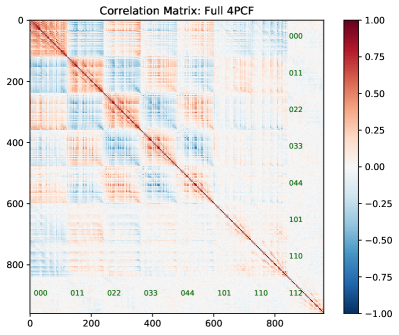
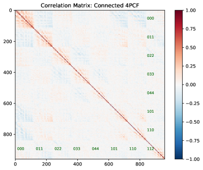
Figure 9: Correlation matrices for the full and connected 4PCFs, as measured from a suite of 1 000 lognormal mocks at $z=2$. The connected 4PCF contribution is computed as the difference between full and disconnected 4PCFs, as in (22). Each $120\times 120$ submatrix contains a single pair of multiplets with $\{\ell_{1},\ell_{2},\ell_{3}\}$ ($\{\ell^{\prime}_{1},\ell^{\prime}_{2},\ell^{\prime}_{3}\}$) indicated in green on the bottom (right) of each matrix. We note that the 4PCF becomes substantially less correlated after subtracting the disconnected piece (which sources the partially-coupled covariance contributions discussed in §VI.3).

References

• [1] N. Bartolo, E. Komatsu, S. Matarrese and A. Riotto, Non-Gaussianity from inflation: theory and observations, Phys. Rep. 402 (2004) 103 [astro-ph/0406398].
• [2] Planck Collaboration, Y. Akrami, F. Arroja, M. Ashdown, J. Aumont, C. Baccigalupi et al., Planck 2018 results. IX. Constraints on primordial non-Gaussianity, A&A 641 (2020) A9 [1905.05697].
• [3] P. Ade, J. Aguirre, Z. Ahmed, S. Aiola, A. Ali, D. Alonso et al., The Simons Observatory: science goals and forecasts, JCAP 2019 (2019) 056 [1808.07445].
• [4] DESI Collaboration, A. Aghamousa, J. Aguilar, S. Ahlen, S. Alam, L. E. Allen et al., The DESI Experiment Part I: Science,Targeting, and Survey Design, arXiv e-prints (2016) arXiv:1611.00036 [1611.00036].
• [5] R. Laureijs, J. Amiaux, S. Arduini, J. L. Auguères, J. Brinchmann, R. Cole et al., Euclid Definition Study Report, arXiv e-prints (2011) arXiv:1110.3193 [1110.3193].
• [6] F. Bernardeau, S. Colombi, E. Gaztañaga and R. Scoccimarro, Large-scale structure of the Universe and cosmological perturbation theory, Phys. Rep. 367 (2002) 1 [astro-ph/0112551].
• [7] P. Gagrani and L. Samushia, Information Content of the Angular Multipoles of Redshift-Space Galaxy Bispectrum, MNRAS 467 (2017) 928 [1610.03488].
• [8] N. Agarwal, V. Desjacques, D. Jeong and F. Schmidt, Information content in the redshift-space galaxy power spectrum and bispectrum, JCAP 2021 (2021) 021 [2007.04340].
• [9] A. Chudaykin and M. M. Ivanov, Measuring neutrino masses with large-scale structure: Euclid forecast with controlled theoretical error, JCAP 2019 (2019) 034 [1907.06666].
• [10] C. Hahn and F. Villaescusa-Navarro, Constraining Mν with the bispectrum. Part II. The information content of the galaxy bispectrum monopole, JCAP 2021 (2021) 029 [2012.02200].
• [11] M. Schmittfull, Y. Feng, F. Beutler, B. Sherwin and M. Y. Chu, Eulerian BAO reconstructions and N -point statistics, Phys. Rev. D 92 (2015) 123522 [1508.06972].
• [12] D. Karagiannis, A. Lazanu, M. Liguori, A. Raccanelli, N. Bartolo and L. Verde, Constraining primordial non-Gaussianity with bispectrum and power spectrum from upcoming optical and radio surveys, MNRAS 478 (2018) 1341 [1801.09280].
• [13] A. Moradinezhad Dizgah, M. Biagetti, E. Sefusatti, V. Desjacques and J. Noreña, Primordial non-Gaussianity from biased tracers: likelihood analysis of real-space power spectrum and bispectrum, JCAP 2021 (2021) 015 [2010.14523].
• [14] Z. Slepian, D. J. Eisenstein, F. Beutler, C.-H. Chuang, A. J. Cuesta, J. Ge et al., The large-scale three-point correlation function of the SDSS BOSS DR12 CMASS galaxies, MNRAS 468 (2017) 1070 [1512.02231].
• [15] Z. Slepian, D. J. Eisenstein, J. A. Blazek, J. R. Brownstein, C.-H. Chuang, H. Gil-Marín et al., Constraining the baryon-dark matter relative velocity with the large-scale three-point correlation function of the SDSS BOSS DR12 CMASS galaxies, MNRAS 474 (2018) 2109 [1607.06098].
• [16] H. Gil-Marín, J. Noreña, L. Verde, W. J. Percival, C. Wagner, M. Manera et al., The power spectrum and bispectrum of SDSS DR11 BOSS galaxies - I. Bias and gravity, MNRAS 451 (2015) 539 [1407.5668].
• [17] D. W. Pearson and L. Samushia, A Detection of the Baryon Acoustic Oscillation features in the SDSS BOSS DR12 Galaxy Bispectrum, MNRAS 478 (2018) 4500 [1712.04970].
• [18] D. Gualdi, H. Gil-Marín, R. L. Schuhmann, M. Manera, B. Joachimi and O. Lahav, Enhancing BOSS bispectrum cosmological constraints with maximal compression, MNRAS 484 (2019) 3713 [1806.02853].
• [19] G. d’Amico, J. Gleyzes, N. Kokron, K. Markovic, L. Senatore, P. Zhang et al., The cosmological analysis of the SDSS/BOSS data from the Effective Field Theory of Large-Scale Structure, JCAP 2020 (2020) 005 [1909.05271].
• [20] H. Gil-Marín, W. J. Percival, L. Verde, J. R. Brownstein, C.-H. Chuang, F.-S. Kitaura et al., The clustering of galaxies in the SDSS-III Baryon Oscillation Spectroscopic Survey: RSD measurement from the power spectrum and bispectrum of the DR12 BOSS galaxies, MNRAS 465 (2017) 1757 [1606.00439].
• [21] Z. Slepian and D. J. Eisenstein, Computing the three-point correlation function of galaxies in O(N2̂) time, MNRAS 454 (2015) 4142 [1506.02040].
• [22] Z. Slepian and D. J. Eisenstein, Accelerating the two-point and three-point galaxy correlation functions using fourier transforms, Monthly Notices of the Royal Astronomical Society: Letters 455 (2015) L31–L35.
• [23] Z. Slepian and D. J. Eisenstein, A practical computational method for the anisotropic redshift-space three-point correlation function, MNRAS 478 (2018) 1468 [1709.10150].
• [24] I. Szapudi, Three-Point Statistics from a New Perspective, ApJ 605 (2004) L89 [astro-ph/0404476].
• [25] L. L. Zhang and U.-L. Pen, Fast n-point correlation functions and three-point lensing application, New. Astron. 10 (2005) 569 [astro-ph/0305447].
• [26] A. W. Moore, A. J. Connolly, C. Genovese, A. Gray, L. Grone, I. Kanidoris, Nick et al., Fast Algorithms and Efficient Statistics: N-Point Correlation Functions, in Mining the Sky, A. J. Banday, S. Zaroubi and M. Bartelmann, eds., p. 71, Jan., 2001, astro-ph/0012333, DOI.
• [27] R. Scoccimarro, Fast estimators for redshift-space clustering, Phys. Rev. D 92 (2015) 083532 [1506.02729].
• [28] K. Garcia and Z. Slepian, Improving the line of sight for the anisotropic 3-point correlation function of galaxies: Centroid and unit-vector-average methods scaling as $\mathcal{O}(n^{2})$, 2020.
• [29] N. S. Sugiyama, S. Saito, F. Beutler and H.-J. Seo, A complete fft-based decomposition formalism for the redshift-space bispectrum, Monthly Notices of the Royal Astronomical Society 484 (2018) 364–384.
• [30] Z. Slepian and D. J. Eisenstein, Modelling the large-scale redshift-space 3-point correlation function of galaxies, Monthly Notices of the Royal Astronomical Society 469 (2017) 2059–2076.
• [31] R. Scoccimarro, The Bispectrum: From Theory to Observations, ApJ 544 (2000) 597 [astro-ph/0004086].
• [32] M. Takada and B. Jain, The three-point correlation function in cosmology, MNRAS 340 (2003) 580 [astro-ph/0209167].
• [33] E. Gaztañaga and R. Scoccimarro, The three-point function in large-scale structure: redshift distortions and galaxy bias, MNRAS 361 (2005) 824 [astro-ph/0501637].
• [34] F. A. Marín, R. H. Wechsler, J. A. Frieman and R. C. Nichol, Modeling the Galaxy Three-Point Correlation Function, ApJ 672 (2008) 849 [0704.0255].
• [35] Z. Slepian and D. J. Eisenstein, Modelling the large-scale redshift-space 3-point correlation function of galaxies, MNRAS 469 (2017) 2059 [1607.03109].
• [36] T. Baldauf, L. Mercolli, M. Mirbabayi and E. Pajer, The bispectrum in the Effective Field Theory of Large Scale Structure, JCAP 2015 (2015) 007 [1406.4135].
• [37] R. E. Angulo, S. Foreman, M. Schmittfull and L. Senatore, The one-loop matter bispectrum in the Effective Field Theory of Large Scale Structures, JCAP 2015 (2015) 039 [1406.4143].
• [38] D. Gualdi, H. Gil-Marín, M. Manera, B. Joachimi and O. Lahav, Geometrical compression: a new method to enhance the BOSS galaxy bispectrum monopole constraints, MNRAS 484 (2019) L29 [1901.00987].
• [39] Z. Slepian, D. J. Eisenstein, J. R. Brownstein, C.-H. Chuang, H. Gil-Marín, S. Ho et al., Detection of baryon acoustic oscillation features in the large-scale three-point correlation function of SDSS BOSS DR12 CMASS galaxies, MNRAS 469 (2017) 1738 [1607.06097].
• [40] Z. Slepian and D. J. Eisenstein, On the signature of the baryon–dark matter relative velocity in the two- and three-point galaxy correlation functions, Monthly Notices of the Royal Astronomical Society 448 (2015) 9–26.
• [41] C. G. Sabiu, B. Hoyle, J. Kim and X.-D. Li, Graph Database Solution for Higher-order Spatial Statistics in the Era of Big Data, ApJS 242 (2019) 29 [1901.00296].
• [42] J. Tomlinson, D. Jeong and J. Kim, Efficient Parallel Algorithm for Estimating Higher-order Polyspectra, AJ 158 (2019) 116 [1904.11055].
• [43] D. Bertolini, K. Schutz, M. P. Solon and K. M. Zurek, The trispectrum in the Effective Field Theory of Large Scale Structure, JCAP 2016 (2016) 052 [1604.01770].
• [44] D. Gualdi, S. Novell, H. Gil-Marín and L. Verde, Matter trispectrum: theoretical modelling and comparison to N-body simulations, JCAP 2021 (2021) 015 [2009.02290].
• [45] D. Gualdi, H. Gil-Marin and L. Verde, Joint analysis of anisotropic power spectrum, bispectrum and trispectrum: application to N-body simulations, arXiv e-prints (2021) arXiv:2104.03976 [2104.03976].
• [46] M. Shiraishi, Parity violation in the CMB trispectrum from the scalar sector, Phys. Rev. D 94 (2016) 083503 [1608.00368].
• [47] O. H. E. Philcox, “Probing Parity-Violation with the BOSS Four-Point Galaxy Correlation Function.” in prep.
• [48] O. H. E. Philcox, Z. Slepian, J. Hou, C. Warner, R. N. Cahn and D. J. Eisenstein, ENCORE: Estimating Galaxy $N$-point Correlation Functions in $\mathcal{O}(N_{\rm g}^{2})$ Time, arXiv e-prints (2021) arXiv:2105.08722 [2105.08722].
• [49] O. H. E. Philcox and Z. Slepian, Efficient Computation of $N$-point Correlation Functions in $D$ Dimensions, arXiv e-prints (2021) arXiv:2106.10278 [2106.10278].
• [50] R. N. Cahn and Z. Slepian, Isotropic N-Point Basis Functions and Their Properties, arXiv e-prints (2020) arXiv:2010.14418 [2010.14418].
• [51] J. Hou, N. Cahn, Robert, O. H. E. Philcox, Z. Slepian and et al., Analytic Gaussian Covariance Matrices for Galaxy $N$-Point Correlation Functions, .
• [52] F. Beutler, H.-J. Seo, S. Saito, C.-H. Chuang, A. J. Cuesta, D. J. Eisenstein et al., The clustering of galaxies in the completed SDSS-III Baryon Oscillation Spectroscopic Survey: anisotropic galaxy clustering in Fourier space, MNRAS 466 (2017) 2242 [1607.03150].
• [53] NIST, NIST Digital Library of Mathematical Functions. DLMF.
• [54] D. A. Varshalovich, A. N. Moskalev and V. K. Khersonskii, Quantum Theory of Angular Momentum. 1988, 10.1142/0270.
• [55] S. D. Landy and A. S. Szalay, Bias and Variance of Angular Correlation Functions, ApJ 412 (1993) 64.
• [56] N. Hand, Y. Feng, F. Beutler, Y. Li, C. Modi, U. Seljak et al., nbodykit: An Open-source, Massively Parallel Toolkit for Large-scale Structure, AJ 156 (2018) 160 [1712.05834].
• [57] J. N. Grieb, A. G. Sánchez, S. Salazar-Albornoz and C. Dalla Vecchia, Gaussian covariance matrices for anisotropic galaxy clustering measurements, MNRAS 457 (2016) 1577 [1509.04293].
• [58] E. Sellentin and A. F. Heavens, Parameter inference with estimated covariance matrices, MNRAS 456 (2016) L132 [1511.05969].
• [59] U.-L. Pen, T. Zhang, L. van Waerbeke, Y. Mellier, P. Zhang and J. Dubinski, Detection of Dark Matter Skewness in the VIRMOS-DESCART Survey: Implications for $\Omega$0, ApJ 592 (2003) 664 [astro-ph/0302031].
• [60] T. L. Smith and M. Kamionkowski, Probability distribution for non-Gaussianity estimators constructed from the CMB trispectrum, Phys. Rev. D 86 (2012) 063009 [1203.6654].
• [61] M. Münchmeyer and K. M. Smith, Higher N -point function data analysis techniques for heavy particle production and WMAP results, Phys. Rev. D 100 (2019) 123511 [1910.00596].
• [62] C. Hahn, F. Beutler, M. Sinha, A. Berlind, S. Ho and D. W. Hogg, Likelihood non-Gaussianity in large-scale structure analyses, MNRAS 485 (2019) 2956 [1803.06348].
• [63] B. Joachimi, Non-linear shrinkage estimation of large-scale structure covariance, MNRAS 466 (2017) L83 [1612.00752].
• [64] R. O’Connell, D. Eisenstein, M. Vargas, S. Ho and N. Padmanabhan, Large covariance matrices: smooth models from the two-point correlation function, MNRAS 462 (2016) 2681 [1510.01740].
• [65] O. H. E. Philcox, D. J. Eisenstein, R. O’Connell and A. Wiegand, RASCALC: a jackknife approach to estimating single- and multitracer galaxy covariance matrices, MNRAS 491 (2020) 3290 [1904.11070].
• [66] D. Wadekar, M. M. Ivanov and R. Scoccimarro, Cosmological constraints from BOSS with analytic covariance matrices, Phys. Rev. D 102 (2020) 123521 [2009.00622].
• [67] A. F. Heavens, R. Jimenez and O. Lahav, Massive lossless data compression and multiple parameter estimation from galaxy spectra, MNRAS 317 (2000) 965 [astro-ph/9911102].
• [68] J. Alsing and B. Wandelt, Generalized massive optimal data compression, MNRAS 476 (2018) L60 [1712.00012].
• [69] O. H. E. Philcox, M. M. Ivanov, M. Zaldarriaga, M. Simonović and M. Schmittfull, Fewer mocks and less noise: Reducing the dimensionality of cosmological observables with subspace projections, Phys. Rev. D 103 (2021) 043508 [2009.03311].
• [70] A. Taylor, B. Joachimi and T. Kitching, Putting the precision in precision cosmology: How accurate should your data covariance matrix be?, MNRAS 432 (2013) 1928 [1212.4359].
• [71] C. Eckart and G. Young, The approximation of one matrix by another of lower rank, Psychometrika 1 (1936) 211.
• [72] J. Hartlap, P. Simon and P. Schneider, Why your model parameter confidences might be too optimistic. Unbiased estimation of the inverse covariance matrix, A&A 464 (2007) 399 [astro-ph/0608064].
• [73] J. Wishart and M. S. Bartlett, The generalised product moment distribution in a normal system, Proceedings of the Cambridge Philosophical Society 29 (1933) 260.
• [74] S. Alam, F. D. Albareti, C. Allende Prieto, F. Anders, S. F. Anderson, T. Anderton et al., The Eleventh and Twelfth Data Releases of the Sloan Digital Sky Survey: Final Data from SDSS-III, ApJS 219 (2015) 12 [1501.00963].
• [75] D. J. Eisenstein, D. H. Weinberg, E. Agol, H. Aihara, C. Allende Prieto, S. F. Anderson et al., SDSS-III: Massive Spectroscopic Surveys of the Distant Universe, the Milky Way, and Extra-Solar Planetary Systems, AJ 142 (2011) 72 [1101.1529].
• [76] K. S. Dawson, D. J. Schlegel, C. P. Ahn, S. F. Anderson, É. Aubourg, S. Bailey et al., The Baryon Oscillation Spectroscopic Survey of SDSS-III, AJ 145 (2013) 10 [1208.0022].
• [77] H. A. Feldman, N. Kaiser and J. A. Peacock, Power-Spectrum Analysis of Three-dimensional Redshift Surveys, ApJ 426 (1994) 23 [astro-ph/9304022].
• [78] O. H. E. Philcox, Cosmology without window functions: Quadratic estimators for the galaxy power spectrum, Phys. Rev. D 103 (2021) 103504 [2012.09389].
• [79] F.-S. Kitaura, S. Rodríguez-Torres, C.-H. Chuang, C. Zhao, F. Prada, H. Gil-Marín et al., The clustering of galaxies in the SDSS-III Baryon Oscillation Spectroscopic Survey: mock galaxy catalogues for the BOSS Final Data Release, MNRAS 456 (2016) 4156 [1509.06400].
• [80] S. A. Rodríguez-Torres, C.-H. Chuang, F. Prada, H. Guo, A. Klypin, P. Behroozi et al., The clustering of galaxies in the SDSS-III Baryon Oscillation Spectroscopic Survey: modelling the clustering and halo occupation distribution of BOSS CMASS galaxies in the Final Data Release, MNRAS 460 (2016) 1173 [1509.06404].
• [81] M. Vargas-Magaña, S. Ho, A. J. Cuesta, R. O’Connell, A. J. Ross, D. J. Eisenstein et al., The clustering of galaxies in the completed SDSS-III Baryon Oscillation Spectroscopic Survey: theoretical systematics and Baryon Acoustic Oscillations in the galaxy correlation function, MNRAS 477 (2018) 1153 [1610.03506].
• [82] M. M. Ivanov, M. Simonović and M. Zaldarriaga, Cosmological parameters from the BOSS galaxy power spectrum, JCAP 2020 (2020) 042 [1909.05277].
• [83] M. Sinha and L. H. Garrison, CORRFUNC - a suite of blazing fast correlation functions on the CPU, MNRAS 491 (2020) 3022 [1911.03545].
• [84] M. J. Wilson, J. A. Peacock, A. N. Taylor and S. de la Torre, Rapid modelling of the redshift-space power spectrum multipoles for a masked density field, MNRAS 464 (2017) 3121 [1511.07799].
• [85] G. Cabass and F. Schmidt, The EFT likelihood for large-scale structure, JCAP 2020 (2020) 042 [1909.04022].
• [86] T. Nishimichi, G. D’Amico, M. M. Ivanov, L. Senatore, M. Simonović, M. Takada et al., Blinded challenge for precision cosmology with large-scale structure: Results from effective field theory for the redshift-space galaxy power spectrum, Phys. Rev. D 102 (2020) 123541 [2003.08277].
• [87] D. Wadekar and R. Scoccimarro, Galaxy power spectrum multipoles covariance in perturbation theory, Phys. Rev. D 102 (2020) 123517 [1910.02914].
• [88] O. H. E. Philcox and D. J. Eisenstein, Estimating covariance matrices for two- and three-point correlation function moments in Arbitrary Survey Geometries, MNRAS 490 (2019) 5931 [1910.04764].
• [89] Y. Kobayashi, T. Nishimichi, M. Takada, R. Takahashi and K. Osato, Accurate emulator for the redshift-space power spectrum of dark matter halos and its application to galaxy power spectrum, Phys. Rev. D 102 (2020) 063504 [2005.06122].
• [90] N. Kaiser, Clustering in real space and in redshift space, MNRAS 227 (1987) 1.
• [91] G. B. Arfken and H. J. Weber, Mathematical methods for physicists 6th ed. 2005.
• [92] O. H. E. Philcox and D. J. Eisenstein, Computing the small-scale galaxy power spectrum and bispectrum in configuration space, MNRAS 492 (2020) 1214 [1912.01010].
• [93] R. O’Connell and D. J. Eisenstein, Large covariance matrices: accurate models without mocks, MNRAS 487 (2019) 2701 [1808.05978].