2Graduate School of AI, KAIST
11email: ygyoon@kaist.ac.kr
Efficient Neural Network Approximation
of Robust PCA for Automated Analysis
of Calcium Imaging Data
Abstract
Calcium imaging is an essential tool to study the activity of neuronal populations. However, the high level of background fluorescence in images hinders the accurate identification of neurons and the extraction of neuronal activities. While robust principal component analysis (RPCA) is a promising method that can decompose the foreground and background in such images, its computational complexity and memory requirement are prohibitively high to process large-scale calcium imaging data. Here, we propose BEAR, a simple bilinear neural network for the efficient approximation of RPCA which achieves an order of magnitude speed improvement with GPU acceleration compared to the conventional RPCA algorithms. In addition, we show that BEAR can perform foreground-background separation of calcium imaging data as large as tens of gigabytes. We also demonstrate that two BEARs can be cascaded to perform simultaneous RPCA and non-negative matrix factorization for the automated extraction of spatial and temporal footprints from calcium imaging data. The source code used in the paper is available at https://github.com/NICALab/BEAR.
Keywords:
Calcium imaging Robust Principal Component Analysis Neural Network Non-negative matrix factorization.1 Introduction
Recent advances in calcium imaging techniques have enabled imaging population neuronal activity across a large volume [21]. State-of-the-art functional imaging methods can generate more than a gigabyte of data per second [2, 6, 23, 25] that is prohibitively large to be analyzed by humans, which necessitates the development of automated analysis algorithms. Furthermore, calcium imaging data suffers from a high level of background fluorescence, which stems from the intrinsic property of calcium indicator molecules. Neurons with a calcium indicator have a certain baseline fluorescence level at rest (i.e., no activity), which becomes brighter by 20 to 40% when there is a single spike. Because most of the neurons are silent at a given time, the images consist of mostly background and a very small portion of foreground, which makes it challenging to identify neurons in calcium imaging data. Therefore, it is desirable to first separate the foreground (i.e., activity) from the backgrounds [13, 17] before applying downstream analysis algorithms, such as image-based neuron detection algorithms [7, 12], NMF-based signal extraction methods [18, 15], and even volume reconstruction [25].
Robust principal component analysis (RPCA) [4] is a promising method for the separation of the foreground in calcium imaging data. Neuronal activities can be separated from the background fluorescence by exploiting that the background is nearly stationary, while the activity is spatiotemporally sparse [25]. The separation can be formulated as the following optimization problem:
| (1) |
where , L, , , and are a data matrix, a low-rank matrix, a sparse matrix, the norm of , and a hyperparameter, respectively. While this problem is known to be computationally intractable, the exact solution can be obtained under weak assumptions through the surrogate optimization as follows [4, 5]:
| (2) |
where is the nuclear norm of , and is the norm of .
However, conventional RPCA based on the principal component pursuit method (PCP) [4] for solving the optimization problem has limited capabilities when it comes to handling extremely large data because it involves singular value decomposition (SVD) of the entire data matrix, which is computationally expensive. In addition, solving the exact optimization problem requires storage of the entire data in the main memory, which is not feasible for large-scale calcium imaging data sets. Thus, many variants of RPCA have been developed to increase the speed [10, 27, 28] or to process large data [8, 19, 24], but it remains a challenge to simultaneously achieve high speed and scalability.
Here, we introduce a Bilinear neural network for Efficient Approximation of RPCA (BEAR) which is a computationally efficient implementation of RPCA as a neural network. BEAR has a number of advantages over conventional RPCA algorithms. It (a) has significantly lower time complexity of than conventional RPCA with time complexity of for single iteration, where and are the sizes of the data along two dimensions and is the rank of which is typically a small integer, (b) can decompose extremely large data, and (c) can be naturally combined with other neural networks for end-to-end training.
2 Methods
2.1 BEAR as a Robust Principal Component Analysis
BEAR is based on the following surrogate optimization:
| (3) |
which is attained by replacing the minimization of in (2) by the maximum rank constraint on . A low-rank representation of the data is obtained by choosing a small integer . The constraint is enforced by setting , where and . We note that is a stronger condition than , and this additional condition allows us to implement the optimization process as training the network shown in Fig. 1a. Furthermore, we imposed an additional constraint on and by setting to reduce the number of trainable parameters and make the training more stable. Thus, the final form of the optimization problem is expressed as
| (4) |
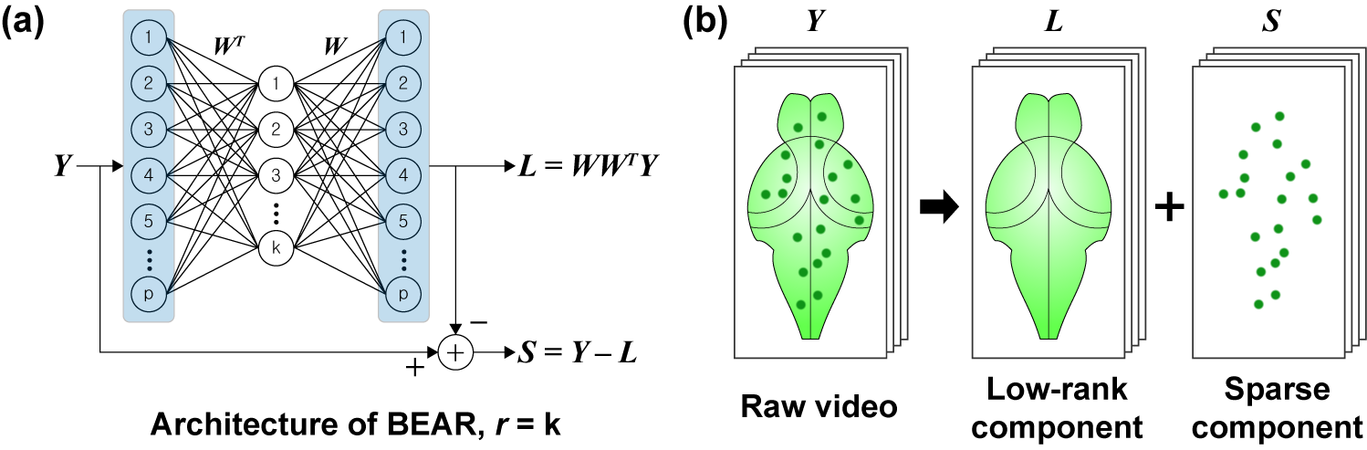
As the three constraints, (a) , (b) , and (c) , are set by the network architecture, the optimization problem can be solved by simply training the network to minimize the loss function (Algorithm S1 in the supplementary material), using gradient-based optimization algorithms, such as stochastic gradient descent, RMSprop [22], and Adam [11]. This allows us to use mini-batches for training the network; hence, it can be applied to an extremely large data matrix . This property is ideal for separating foregrounds in large-scale calcium imaging data (Fig. 1b). It should be noted that both forward propagation and backpropagation through the network require only two matrix multiplications thereby achieving the computational complexity of , whereas other methods that employ SVD have the computational complexity of . Furthermore, the network can be used to infer the low-rank components without updating , assuming that the network is trained with the earlier data points and the low-rank components remain stationary. This inference-only mode can significantly improve the computation time.
2.2 Extensions of BEAR
2.2.1 BEAR with greedy rank estimation.
BEAR requires the integer number to be explicitly set which has to come from prior knowledge regarding the rank of the low-rank matrix , whereas general RPCA methods do not. To employ BEAR in the absence of such prior knowledge, we introduce an extension of BEAR with greedy rank estimation (Greedy BEAR).
Rank estimation is done by adding an outer loop to BEAR in which the target rank is gradually increased. As soon as increases, where is the target rank and is the loss after training the BEAR with the target rank, the algorithm terminates, and the network from the earlier iteration of the outer loop is chosen as the final model. Note that this algorithm (Algorithm S2 in the supplementary material) attempts to solve , which is similar to the original optimization problem expressed in (1).
2.2.2 BEAR as non-negative matrix factorization.
We note that BEAR can be modified to solve non-negative matrix factorization (NMF) by changing the loss function and introducing a non-negativity constraint on as follows:
| (5) |
This optimization problem is equivalent to projective NMF [26]. It is known to produce localized sparse footprints, which is ideal for neuron segmentation.
2.2.3 BEAR cascaded with downstream networks.
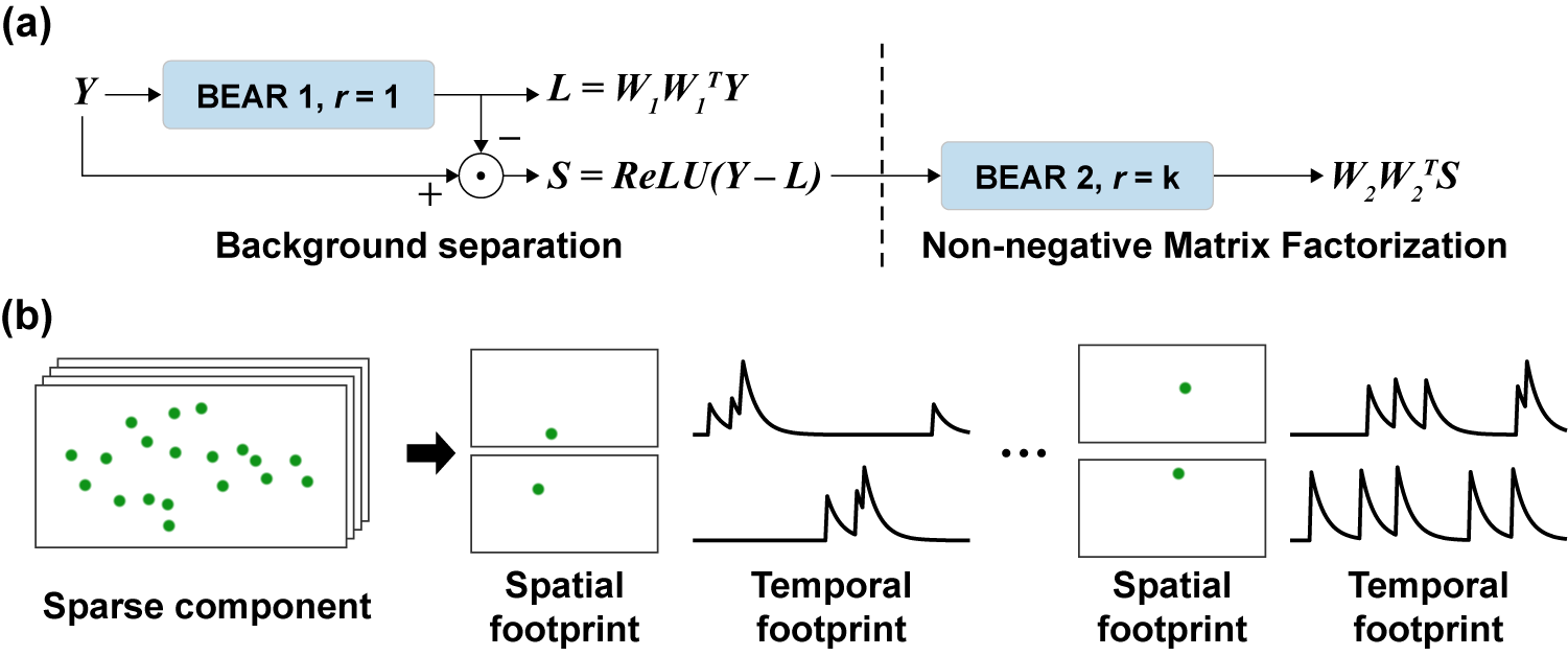
Because BEAR is a neural network, it can be combined with other networks for downstream tasks and trained end-to-end. This can be implemented by cascading BEAR with another network (Cascaded BEAR). The loss function can be set as , where and are the loss functions of the first and second networks, respectively, and is a hyperparameter. As an example, two BEARs can be cascaded to simultaneously perform RPCA and NMF as shown in Fig. 2a. The sparse component from the first BEAR is fed to a ReLU layer to ensure non-negativity and then fed to the second BEAR for NMF (Algorithm S3 in the supplementary material) to extract the spatial and temporal footprints as illustrated in Fig. 2b.
3 Experiments
To validate and evaluate our algorithm, we compared Greedy BEAR with existing RPCA algorithms, PCP [4], IALM [14], GreGoDec [28] and OMWRPCA [24]. Next, we applied the cascaded BEAR to calcium imaging datasets to demonstrate its capability to perform RPCA and NMF simultaneously. We ran these tests on a PC with Intel i7-9700K CPU, NVIDIA GeForce RTX 2080 Ti GPU, and 128GB of RAM. The source code of PCP, IALM, and GreGoDec was from LRSLibrary [3, 20], a publicly available repository of multiple RPCA algorithms. The source code of OMWRPCA was from [24]. PCP, IALM, GreGoDec, and OMWRPCA were run on the CPU. BEAR was implemented using Pytorch, and its performance on the GPU and the CPU was tested separately. The computation time of BEAR includes the time taken for both training and inference. The default maximum number of iterations of PCP was reduced by a factor of 10. The animal experiments conducted for this study were approved by the Institutional Animal Care and Use Committee (IACUC) of KAIST (KA2019‐13).
3.1 Phase diagram in rank and sparsity
We evaluated the ability of the algorithms to recover varying rank matrices from data matrices that have error with varying levels of sparsity. We randomly generated each data matrix by adding a low-rank matrix and a sparse matrix , where was set as 1,000. Each low rank matrix was generated as , where the entities of and were drawn from a normal distribution with the mean value of zero and the variance of . Each sparse matrix was generated by drawing each entity from a probability mass function as follows: .
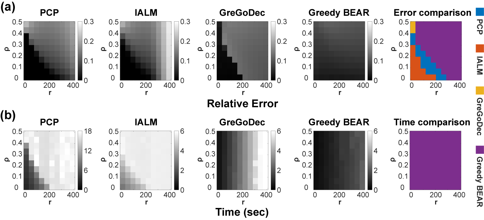
For each (, ) pair, we generated 5 random matrices, each of which was solved with the four algorithms. The evaluation metrics were the relative error, defined as where was the recovered low-rank matrix, and the computation time. We averaged the relative error and computation time from 5 trials for each (, ) pair. We used the Adam optimizer with the batch size of . The learning rate was , and the number of training epochs was .
Figure 3 shows the obtained phase diagrams. Greedy BEAR achieved a relatively uniform level of error across a wide range of and , while other algorithms failed in the high-rank or low-sparsity phase (Fig. 3a). Greedy BEAR was the fastest under all conditions (Fig. 3b). In the rightmost plots in Fig. 3, each grid, which represents each (, ) pair, is assigned to the best algorithm in terms of each measure. The percentages of (, ) pairs which Greedy BEAR achieved the best relative error and the computation time were 69% and 100%, respectively.
3.2 Performance on large calcium imaging data
We measured the computation times of the algorithms using 3-D calcium imaging data. The data was acquired by performing calcium imaging of larval zebrafish brains at 4 Hz using a custom-designed epi-fluorescence microscope. The larvae expressing GCaMP7a pan-neuronally were imaged at 4 days post fertilization. The larvae were paralyzed in standard fish water containing of pancuronium bromide for 2 minutes prior to imaging and then embedded in agarose for immobilization.
| algorithms | PCP | IALM | GreGoDec | OMWRPCA | Greedy BEAR | BEAR† | |
| data size | CPU | CPU | CPU | CPU | CPU | GPU | GPU |
| 13814 | 1211 | 429 | 37883** | 371 | 134 | 42 | |
| OOM* | OOM* | OOM* | 80883** | 1345 | 537 | 377 | |
The sizes of the videos were and , respectively, and they were reshaped to (3.2GB) and (21.3GB), respectively. For BEAR with inference-only mode, the network was trained with the first one third of the data, and inference was performed on the entire data. We used the Adam optimizer with the batch size of . The learning rate was , and the number of training epochs was .
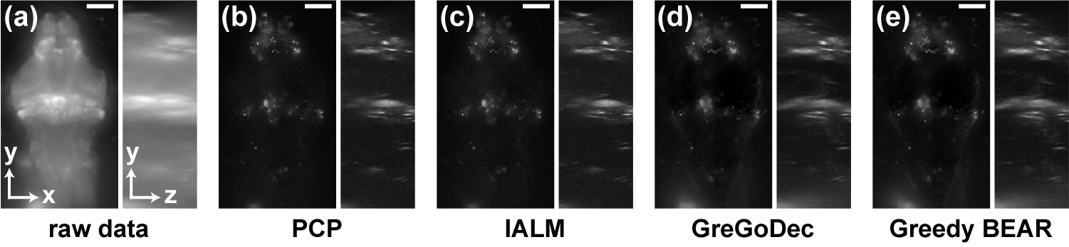
The computation times of the four algorithms are summarized in Table 1. Greedy BEAR with GPU acceleration was faster than the existing algorithms and was capable of processing the largest data. The decomposition results obtained by the four algorithms were visually nearly indistinguishable as shown in Fig. 4 and Supplementary Video 1.
3.3 Simultaneous RPCA and NMF using cascaded BEAR
We applied cascaded BEAR illustrated in Fig. 2a to the publicly available mouse brain calcium imaging data obtained by two-photon microscopy [9] for simultaneous RPCA and NMF. The dimensions of the video were , which were reshaped to . The ranks for the first and second BEARs were set as 1 and 8, respectively. We used the Adam optimizer with the batch size of . The learning rate was and the number of training epochs was 5,000. As shown in Fig. 5, the spatial components from cascaded BEAR were confined and sparse, whereas those from conventional NMF [1, 16] were not. In addition, the temporal signals from cascaded BEAR showed lower baseline fluctuation due to less signal mixing.
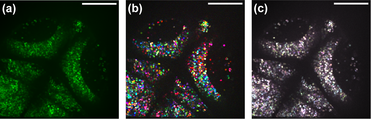
Next, we applied cascaded BEAR to a zebrafish calcium imaging video (Fig. 6a). It was acquired by imaging a larval zebrafish brain, expressing nuclear localized GCaMP6s pan-neuronally, at 10 Hz using a spinning disk confocal microscope with a 25x 1.1NA objective lens. The dimensions of the video were , which were reshaped to . The ranks for the first BEAR and second BEAR were set as 1 and 50, respectively. We used the Adam optimizer with the batch size of . The learning rate was , and the number of training epochs was 1,000. As shown in Fig. 6, cascaded BEAR was able to process the calcium imaging data with a very large number of neurons. The obtained spatial footprints were confined and they corresponded well with the neurons (Fig. 6b), whereas the results obtained by conventional NMF were not confined, which manifested as low color contrast (Fig. 6c).

4 Conclusion
In summary, we proposed BEAR, a bilinear neural network for analyzing large calcium imaging data. Because BEAR can be trained using the gradient from mini-batches, it can decompose arbitrary sized data while exploiting GPU acceleration for speed improvement. Furthermore, BEAR can be cascaded with other networks for end-to-end training. For example, two BEARs can be cascaded for simultaneous RPCA and NMF to identify neurons in a large calcium imaging data. Although our demonstration was focused on processing calcium imaging data, BEAR could be used for other general RPCA applications.
4.0.1 Acknowledgements.
This research was supported by National Research Foundation of Korea (2020R1C1C1009869), the Korea Medical Device Development Fund grant funded by the Korea government (202011B21-05), Institute of Information & communications Technology Planning & Evaluation (IITP) grant funded by the Korea government (MSIT) (No.2019-0-00075, Artificial Intelligence Graduate School Program (KAIST)), and 2020 KAIST-funded AI Research Program. The zebrafish lines used for calcium imaging were provided by the Zebrafish Center for Disease Modeling (ZCDM), Korea.
References
- [1] Berry, M.W., Browne, M., Langville, A.N., Pauca, V.P., Plemmons, R.J.: Algorithms and applications for approximate nonnegative matrix factorization. Computational statistics & data analysis 52(1), 155–173 (2007)
- [2] Bouchard, M.B., Voleti, V., Mendes, C.S., Lacefield, C., Grueber, W.B., Mann, R.S., Bruno, R.M., Hillman, E.M.: Swept confocally-aligned planar excitation (scape) microscopy for high-speed volumetric imaging of behaving organisms. Nature photonics 9(2), 113–119 (2015)
- [3] Bouwmans, T., Sobral, A., Javed, S., Jung, S.K., Zahzah, E.H.: Decomposition into low-rank plus additive matrices for background/foreground separation: A review for a comparative evaluation with a large-scale dataset. Computer Science Review 23, 1–71 (2017)
- [4] Candès, E.J., Li, X., Ma, Y., Wright, J.: Robust principal component analysis? Journal of the ACM (JACM) 58(3), 1–37 (2011)
- [5] Chandrasekaran, V., Sanghavi, S., Parrilo, P.A., Willsky, A.S.: Rank-sparsity incoherence for matrix decomposition. SIAM Journal on Optimization 21(2), 572–596 (2011)
- [6] Cong, L., Wang, Z., Chai, Y., Hang, W., Shang, C., Yang, W., Bai, L., Du, J., Wang, K., Wen, Q.: Rapid whole brain imaging of neural activity in freely behaving larval zebrafish (danio rerio). Elife 6, e28158 (2017)
- [7] Dong, M., Liu, D., Xiong, Z., Chen, X., Zhang, Y., Zha, Z.J., Bi, G., Wu, F.: Towards neuron segmentation from macaque brain images: A weakly supervised approach. In: Martel, A.L., Abolmaesumi, P., Stoyanov, D., Mateus, D., Zuluga, M.A., Zhou, S.K., Racoceanu, D., Joskowicz, L. (eds.) MICCAI 2020. pp. 194–203. LNCS, Springer, Cham (2020)
- [8] Feng, J., Xu, H., Yan, S.: Online robust pca via stochastic optimization. Advances in neural information processing systems 26, 404–412 (2013)
- [9] Giovannucci, A., Friedrich, J., Gunn, P., Kalfon, J., Brown, B.L., Koay, S.A., Taxidis, J., Najafi, F., Gauthier, J.L., Zhou, P., et al.: Caiman an open source tool for scalable calcium imaging data analysis. Elife 8, e38173 (2019)
- [10] Hovhannisyan, V., Panagakis, Y., Parpas, P., Zafeiriou, S.: Multilevel approximate robust principal component analysis. In: Proceedings of the IEEE International Conference on Computer Vision Workshops. pp. 536–544 (2017)
- [11] Kingma, D.P., Ba, J.: Adam: A method for stochastic optimization. arXiv preprint arXiv:1412.6980 (2014)
- [12] Kirschbaum, E., Bailoni, A., Hamprecht, F.A.: Disco: Deep learning, instance segmentation, and correlations for cell segmentation in calcium imaging. In: Martel, A.L., Abolmaesumi, P., Stoyanov, D., Mateus, D., Zuluga, M.A., Zhou, S.K., Racoceanu, D., Joskowicz, L. (eds.) MICCAI 2020. pp. 151–162. LNCS, Springer, Cham (2020)
- [13] Li, C., Li, X., Cao, H., Jiang, H., Deng, X., Chen, D.Z., Yang, L., Shao, Z.: Fast background removal method for 3d multi-channel deep tissue fluorescence imaging. In: Descoteaux, M., Maier-Hein, L., Franz, A., Jannin, P., Collins, D.L., Duchesne, S. (eds.) MICCAI 2017. LNCS, vol. 10434, pp. 92–99. Springer, Cham (2017)
- [14] Lin, Z., Chen, M., Ma, Y.: The augmented lagrange multiplier method for exact recovery of corrupted low-rank matrices. arXiv preprint arXiv:1009.5055 (2010)
- [15] Nejatbakhsh, A., Varol, E., Yemini, E., Venkatachalam, V., Lin, A., Samuel, A.D., Hobert, O., Paninski, L.: Demixing calcium imaging data in c. elegans via deformable non-negative matrix factorization. In: Martel, A.L., Abolmaesumi, P., Stoyanov, D., Mateus, D., Zuluga, M.A., Zhou, S.K., Racoceanu, D., Joskowicz, L. (eds.) MICCAI 2020. LNCS, vol. 12265, pp. 14–24. Springer, Cham (2020)
- [16] Paatero, P., Tapper, U.: Positive matrix factorization: A non-negative factor model with optimal utilization of error estimates of data values. Environmetrics 5(2), 111–126 (1994)
- [17] Peng, T., Wang, L., Bayer, C., Conjeti, S., Baust, M., Navab, N.: Shading correction for whole slide image using low rank and sparse decomposition. In: Golland, P., Hata, N., Barillot, C., Hornegger, J., Howe, R. (eds.) MICCAI 2014. LNCS, vol. 8673, pp. 33–40. Springer, Cham (2014)
- [18] Pnevmatikakis, E.A., Soudry, D., Gao, Y., Machado, T.A., Merel, J., Pfau, D., Reardon, T., Mu, Y., Lacefield, C., Yang, W., et al.: Simultaneous denoising, deconvolution, and demixing of calcium imaging data. Neuron 89(2), 285–299 (2016)
- [19] Rahmani, M., Atia, G.K.: High dimensional low rank plus sparse matrix decomposition. IEEE Transactions on Signal Processing 65(8), 2004–2019 (2017)
- [20] Sobral, A., Bouwmans, T., Zahzah, E.h.: Lrslibrary: Low-rank and sparse tools for background modeling and subtraction in videos. Robust Low-Rank and Sparse Matrix Decomposition: Applications in Image and Video Processing (2016)
- [21] Stevenson, I.H., Kording, K.P.: How advances in neural recording affect data analysis. Nature neuroscience 14(2), 139–142 (2011)
- [22] Tieleman, T., Hinton, G.: Lecture 6.5-rmsprop: Divide the gradient by a running average of its recent magnitude. COURSERA: Neural networks for machine learning 4(2), 26–31 (2012)
- [23] Voleti, V., Patel, K.B., Li, W., Campos, C.P., Bharadwaj, S., Yu, H., Ford, C., Casper, M.J., Yan, R.W., Liang, W., et al.: Real-time volumetric microscopy of in vivo dynamics and large-scale samples with scape 2.0. Nature methods 16(10), 1054–1062 (2019)
- [24] Xiao, W., Huang, X., He, F., Silva, J., Emrani, S., Chaudhuri, A.: Online robust principal component analysis with change point detection. IEEE Transactions on Multimedia 22(1), 59–68 (2019)
- [25] Yoon, Y.G., Wang, Z., Pak, N., Park, D., Dai, P., Kang, J.S., Suk, H.J., Symvoulidis, P., Guner-Ataman, B., Wang, K., et al.: Sparse decomposition light-field microscopy for high speed imaging of neuronal activity. Optica 7(10), 1457–1468 (2020)
- [26] Yuan, Z., Yang, Z., Oja, E.: Projective nonnegative matrix factorization: Sparseness, orthogonality, and clustering. Neural Process. Lett pp. 11–13 (2009)
- [27] Zhou, T., Tao, D.: Godec: Randomized low-rank & sparse matrix decomposition in noisy case. In: Proceedings of the 28th International Conference on Machine Learning, ICML 2011 (2011)
- [28] Zhou, T., Tao, D.: Greedy bilateral sketch, completion & smoothing. In: AISTATS. vol. 31, pp. 650–658. PMLR (2013)