Computation of Gravitational Particle Production Using Adiabatic Invariants

Abstract

Analytic and numerical techniques are presented for computing gravitational production of scalar particles in the limit that the inflaton mass is much larger than the Hubble expansion rate at the end of inflation. These techniques rely upon adiabatic invariants and time modeling of a typical inflaton field which has slow and fast time variation components. A faster computation time for numerical integration is achieved via subtraction of slowly varying components that are ultimately exponentially suppressed. The fast oscillatory remnant results in production of scalar particles with a mass larger than the inflationary Hubble expansion rate through a mechanism analogous to perturbative particle scattering. An improved effective Boltzmann collision equation description of this particle production mechanism is developed. This model allows computation of the spectrum using only adiabatic invariants, avoiding the need to explicitly solve the inflaton equations of motion.

I Introduction

Gravitational production of superheavy hidden sector particles during the transition out of the inflationary quasi-de Sitter (quasi-dS) era remains a plausible mechanism of dark matter production (e.g. [1, 2, 3, 4, 5, 6, 7, 8, 9, 10, 11, 12, 13, 14, 15]). However, gravitational production of super-Hubble-mass particles was largely considered phenomenologically uninteresting due to an exponential suppression during inflation. This outlook has changed after it was found [29, 30, 8] that unsuppressed production can take place after inflation via

$$\mbox{coherent oscillating inflatons }\phi\rightarrow\mbox{graviton}\rightarrow\chi\mbox{ particles }$$ (1)

for some inflationary models if $m_{\phi}>m_{\chi}\gg H_{\mathrm{inf}}$, where $H_{\mathrm{inf}}$ is the inflationary Hubble expansion rate, and $m_{\phi}$ and $m_{\chi}$ are the masses of the respective particles. For example, this can occur in hilltop models such as those of refs. [31, 32, 33, 34, 15].

Intuitively, the fast oscillatory component in an otherwise slow Hubble expansion rate $H$ after the quasi-dS era leads to the production of particles. In contrast with preheating related particle production (e.g.  [35, 36, 37, 38, 39, 40]), this scenario requires mediation by the massless gravitational sector, which cannot be integrated out. Also, unlike the scenarios of refs. [27, 41, 42, 43], the phase space structure of the initial inflaton degrees of freedom is fixed by the Bunch-Davies/adiabatic vacuum prescription during inflation. It is in this sense that the particle production considered in ref. [8] might naively be thought of as part of the gravitational particle production resulting from the transition out of the quasi-dS era.

In ref. [44], an analytic formalism for computing the particle production in this scenario was constructed based on a double expansion in $H/m_{\phi}\ll 1$ and $H/m_{\chi}\ll 1$. In using the formalism, a Gaussian spectral model was introduced to obtain a compact formula. It was based on the assumptions that the Fourier spectrum of the fast time variation of the inflaton field is approximately Gaussian, and that most of the particle production takes place during the first few oscillations. A production rate was then estimated using a naive matching to the Fermi’s golden rule, and the Boltzmann equation was integrated to obtain the final number density.

However, there were at least two problems with this. Firstly, the matching to Fermi’s golden rule was done in a non-systematic manner, and neglected the long time behavior of the dynamics, although it certainly is correct to $O(1)$ accuracy. Secondly, the high $k$ part of the particle production spectrum requires the fast oscillation component of $H$ to be tracked for longer than a few oscillation periods. This is because the time $t_{*}$ at which the time-integral in the formalism picks up the dominant contribution to the particle production amplitude is when

$$\frac{k^{2}}{a^{2}(t_{*})}+m_{\chi}^{2}\approx m_{\phi}^{2},$$ (2)

corresponding to the on-shell condition of eq. (1).

One of the main results of this paper is to correct these shortcomings. More specifically, using the technique of adiabatic invariants, we construct an accurate time model instead of a spectral model. We will see that these will lead to a 2+$O(1)$ factor correction to the final spectrum compared to that of ref. [44].

It is important to note that the adiabatic invariant formalism of this paper is distinct from the adiabatic vacuum of refs. [45, 46, 47]. In particular, the latter is essentially the WKB approximation, and applies only to linear wave equations, while the former requires oscillatory motion, and can be applied to non-linear Hamiltonian dynamics. Furthermore, in the context of gravitational particle production, the WKB approach is used to solve the $\chi_{k}$ mode equation, and is controlled by an expansion in $H/m_{\chi}$. In contrast, the adiabatic invariant formalism of this paper is used to analyze the dynamics of the inflaton $\phi$ and the scale factor $a$, and is controlled by $H/m_{\phi}$. This then determines the $\chi$ mode dispersion, which controls its particle production.

A second main result of this paper demonstrates that one can use the formalism of ref. [44] to compute the spectrum numerically more efficiently than the brute force methods used in the literature. We note that what is expensive to compute numerically is the slow time-varying component weighted integration over fast oscillating functions which converge slowly to a negligible contribution. Instead, the formalism of ref. [44] already isolates the fast time variation such that its numerical integration can be more than $O(1000)$ faster in convergence. The relative gain in efficiency depends on the amplitude of the spectrum.

It is important to note that although the original motivation for this scenario is the production of dark matter, the computational tools presented in this work are useful for constraining top down constructions as well. For example, in contrast with moduli problem scenarios such as those of refs. [48, 49], moduli much heavier than the inflationary expansion rate can be gravitationally produced as well during the first few oscillations out of inflation [50] (where the largest number is produced in the first oscillation). Furthermore, even if the particles decay too rapidly to be dark matter, they can have observable consequences as long as they are sufficiently long lived, as discussed for example in refs. [2, 51, 5, 52, 53, 54, 55, 56, 57, 58, 59, 60].

The order of presentation will be as follows. In section II, we summarize the previous work of separating the $H$ time scale from the $m_{\phi}$ time scale and explain its shortcomings [44]. Here, we also establish the notation for this paper. In section III, we explain how the adiabatic invariant can be constructed and how to use it to compute the long time behavior of slowly varying fields. This tool will play a crucial role in section IV, where we present a more accurate approximation of the Boltzmann equation, which is one of the main goals of this paper. We parameterize the associated errors based on a coarse graining over short time scales. In section V, we introduce an explicit time model of the inflaton dynamics that separates the short and long time scale dependences.

In section VI, we derive an analytic formula for the coarse grained particle production amplitude that includes $\{1\rightarrow 2,2\rightarrow 2,3\rightarrow 2\}$ resonance contributions. The formulae of this section are analogous to the S-matrix amplitude, which will need to be supplemented with an analog of phase space integrals to express a physically measurable number density. The coarse graining time scale is computed in section VII by minimizing the competing errors associated with quantum interference and general sum to integral approximations. We calculate the spectrum and number density estimates in section VIII by utilizing the explicit solutions obtained from the adiabatic invariant tool. In section IX, we present our second main result: numerical integration advantage of the “fast only” formula of eq. (162) over the brute force Bogoliubov formulation of eq. (8). In that section, we also generalize the Gaussian spectral model of ref. [44] by incorporating the adiabatic invariant formalism, and compare it with other computational methods.

We summarize our results in section X. The appendices include a review of the adiabatic invariant formalism used in this paper and a derivation of an explicit formula for the time dependence of the slowly varying Hubble expansion rate after the end of inflation for a generic inflationary potential.

II Aspects of previous work on the topic

Here we review our conventions and previous work on this topic. Consider the action in the metric signature (1,-1,-1,-1):

$$S=\int d^{4}x\sqrt{-g}\left(-\frac{M_{P}^{2}}{2}R+\frac{1}{2}g^{\mu\nu}\partial_{\mu}\phi\partial_{\nu}\phi-V(\phi)+\frac{1}{2}g^{\mu\nu}\partial_{\mu}\chi\partial_{\nu}\chi-\frac{1}{2}\left(m_{\chi}^{2}-\xi R\right)\chi^{2}\right),$$ (3)

where $M_{P}=1/\sqrt{8\pi G}$ is the reduced Planck mass, $R$ is the Ricci scalar, $\phi$ denotes the inflaton field with potential $V(\phi)$, and $\chi$ denotes a real scalar field. We assume that $\chi$ interacts only through gravity controlled by a non-minimal coupling $\xi$. Pure Einstein gravity (i.e. minimal coupling) corresponds to $\xi=0$ while conformal coupling corresponds to $\xi=1/6$. The standard background cosmological metric is written as

$$ds^{2}=g_{\mu\nu}dx^{\mu}dx^{\nu}=dt^{2}-a^{2}(t)\left|d\vec{x}\right|^{2}=a^{2}(\tau)\left(d\tau^{2}-\left|d\vec{x}\right|^{2}\right),$$ (4)

where the scalar factor $a$ is a function of either coordinate time $t$ or conformal time $\tau$. The Hubble parameter $H$ and Ricci scalar $R$ have the conventions

$$H=\frac{\dot{a}}{a}=\frac{a^{\prime}}{a^{2}}\qquad\text{and}\qquad R=-6\left(\frac{\ddot{a}}{a}+\frac{\dot{a}^{2}}{a^{2}}\right)=-6\frac{a^{\prime\prime}}{a^{3}},$$ (5)

where $\dot{a}=\partial_{t}a$ and $a^{\prime}=\partial_{\tau}a$. The energy-momentum tensor is assumed to arise primarily from a homogeneous inflaton field $\phi$, and therefore Einstein’s equation can be written as

$$3M_{P}^{2}H^{2}=\rho\simeq\frac{1}{2}\dot{\phi}^{2}+V(\phi)\qquad\text{and}\qquad-M_{P}^{2}R=\rho-3P\simeq-\dot{\phi}^{2}+4V(\phi).$$ (6)

It is well known that the number density $n_{\chi}$ can be written as

$$a^{3}(t)n_{\chi}(t)=\int\frac{d^{3}k}{(2\pi)^{3}}\,f_{\chi}(k,t),\qquad f_{\chi}(k,t)\equiv\left|\beta_{k}(t)\right|^{2},$$ (7)

where the Bogoliubov coefficient expression for gravitational production of $\chi$ particles with mass $m_{\chi}$ is

$$\beta_{k}(t)=\int_{-\infty}^{t}dt^{\prime}\frac{\dot{\omega}_{k}(t^{\prime})}{2\omega_{k}(t^{\prime})}e^{-2i\int_{-\infty}^{t^{\prime}}dt^{\prime\prime}\frac{\omega_{k}(t^{\prime\prime})}{a(t^{\prime\prime})}},$$ (8)

with $\omega_{k}^{2}\equiv k^{2}+a^{2}m_{\chi}^{2}+\frac{1}{6}(1-6\xi)a^{2}R$ as long as $|\beta_{k}|\ll 1$ [62, 38]. After separating out the time scale much faster than $H^{-1}$, the expression can be written as

$$\beta_{k}(t)\approx\int_{t_{\mathrm{end}}}^{t}dt^{\prime}\,B_{k}(t^{\prime})e^{-2i\Omega_{k}(t^{\prime})},$$ (9)

where $t_{\mathrm{end}}$ is the time when inflation ends (when the slow-roll parameter $\epsilon$ is unity), with

$$E_{k}^{2}(t) \equiv\frac{k^{2}}{a_{\mathrm{slow}}^{2}(t)}+m_{\chi}^{2},$$ (10)

$$\Omega_{k}(s) \equiv\int_{t_{\mathrm{end}}}^{s}E_{k}(s^{\prime})ds^{\prime},$$ (11)

$$B_{k}(t) =\left(\frac{H_{\mathrm{UV}}(t)}{2}+\frac{1}{24}\left(1-6\xi\right)\frac{\dot{R}_{\mathrm{UV}}(t)}{m_{\chi}^{2}}\right)\frac{m_{\chi}^{2}}{E_{k}^{2}(t)},$$ (12)

and the subscript UV denotes the quantities with the low frequency components filtered out [44]. In the work of ref. [44], a Gaussian Fourier spectrum function with a high frequency peak was fit to the properties of the potential to effectively define these UV components. Although this did allow one to analytically compute the dominant contribution to the particle production in a clean formula, there were some shortcomings:

1. Although the largest amplitude of inflaton oscillations occurs at $t_{\mathrm{end}}$, particle production remains significant at later times when the amplitude is appreciably smaller. Indeed, the final number density was computed in that reference by converting the first few oscillations computation into a rate using

   $$\frac{d\gamma(t_{\mathrm{end}})}{dk}\equiv\frac{\sigma}{\sqrt{2\pi}}\left.\frac{dn_{\chi}}{dk}\right|_{t_{\mathrm{end}}+\frac{\sqrt{2\pi}}{\sigma}},$$ (13)

   (where $\sigma$ is related to the Gaussian spectral model), setting $t_{\mathrm{end}}\rightarrow t$, and using a Boltzmann equation to compute the production rate. However, no formalism was provided on how to solve for the long time scale dependence such that the replacement $t_{\mathrm{end}}\rightarrow t$ can be made for an inflaton potential that is not purely quadratic. One expects this long time scale to be particularly important for the $k$ modes where

   $$\frac{k}{a_{\mathrm{end}}}\gg\sqrt{m_{\phi}^{2}-m_{\chi}^{2}}\gg H,\qquad a_{\mathrm{end}}\equiv a(t_{\mathrm{end}}),$$ (14)

   since for these cases, $\beta_{k}$ settles to its asymptotic final value only for $t\gg t_{\mathrm{end}}$.

2. The choice of the coarse graining time scale identification $\left(\Delta t\right)^{-1}=\sigma/\sqrt{2\pi}$ in equation 6.11 of ref. [44] was an estimate for the coarse graining time scale based on the naive expectation of the Gaussian frequency model:

   $$\delta(E_{*}-E_{*}) =\lim_{\sigma^{2}\rightarrow 0}\frac{1}{\sqrt{2\pi\sigma^{2}}}\exp[-(E_{*}-E_{*})^{2}/(2\sigma^{2})],$$ (15)

   $$\frac{\Delta t}{2\pi} =\lim_{\sigma^{2}\rightarrow 0}\frac{1}{\sqrt{2\pi\sigma^{2}}}.$$ (16)

   However, since the actual Gaussian model comes from the square of $\dot{\phi}^{2}$ whereas eq. (16) came from the $\phi$ spectral representation itself (see equation 5.23 of ref. [44]), there is an ambiguity in this identification.

Both of these shortcomings will be addressed in this paper through a novel time dependent model based on an adiabatic invariant construction replacing the Gaussian Fourier spectral model of ref. [44]. The use of the adiabatic invariant also makes more precise exactly which $\dot{\phi}^{2}$ component is being kept when evaluating $\beta_{k}$ contributions from “fast varying” (UV) modes.

III Constructing the adiabatic invariant

One of the issues outlined near eq. (14) is the long time scale behavior of the inflaton oscillation amplitude necessary for the accurate determination of the amplitude for the high $k$ modes. To compute this, we use the adiabatic invariant technique reviewed in appendix A. This technique allows one to construct an approximate invariant $Q$ because of the combination of the properties that Hamiltonian equations of motion preserving phase space and energy being conserved in the limit that an external time-translation breaking function becomes a constant.

To use the adiabatic invariant to isolate the slowly varying part from the fast varying part of $T^{\mu\nu}$ cleanly, we decompose the FLRW scale factor as $a(t)=a_{\mathrm{slow}}(t)+a_{\mathrm{fast}}(t)$. Let the slowly varying source function for the adiabatic invariant construction be $\lambda(t)=a_{\mathrm{slow}}(t)$ and let the coordinate of the phase space $q$ (in the notation of the appendix A) be the inflaton field $\phi$. An interesting part of the procedure we are going to follow is that $a_{\mathrm{slow}}(t)$ does not need to be specified to obtain the adiabatic invariant.

We start by carrying out the integral in eq. (207). We choose $C$ to be the $\phi$ path that begins and ends at $\phi(v)$. We can set the initial condition $\phi(v)$ at which $\pi(v)=0$. This can typically be done since the motion is oscillatory by assumption and the turning point typically corresponds to $\pi=0$. We can therefore write $E(v)$ from eq. (186) as

$$E(v)=H\left(\phi^{\prime},\Pi\left[\phi^{\prime},E(v),a_{\mathrm{slow}}(v)\right],a_{\mathrm{slow}}(v)\right)=H(\phi^{\prime},0,a_{\mathrm{slow}}(v)),$$ (17)

where $H$ is the Hamiltonian and $\phi^{\prime}$ is any field value in the path $C$. This results in an adiabatic invariant equation for $\phi(v)$:

$$Q=\oint_{C}d\phi^{\prime}\Pi[\phi^{\prime},H(\phi(v),0,a_{\mathrm{slow}}(v)),a_{\mathrm{slow}}(v)],$$ (18)

Since this expression is a constant, we have a prediction for how $\phi(v)$ varies as a function of $a_{\mathrm{slow}}(v)$.

Let us now obtain a more explicit expression for $\phi(v)$ using the conservation of energy per integration cycle $\oint_{C}d\phi$. First, canonically normalize the fields such that the Lagrangian is $a_{\mathrm{slow}}^{3}(t)[\tfrac{1}{2}\dot{\phi}^{2}-V(\phi)].$ If there are non-minimal gravitational couplings, such terms can be absorbed into $V$. The momentum conjugate to $\phi$ is $\pi=a_{\mathrm{slow}}^{3}\dot{\phi}$, and thus the Hamiltonian is

$$H(\phi,\pi,a_{\mathrm{slow}})=\frac{1}{2}\frac{\pi^{2}}{a_{\mathrm{slow}}^{3}}+a_{\mathrm{slow}}^{3}V(\phi).$$ (19)

Solving for $\Pi$ using eqs. (17) and (19), the adiabatic invariant can now be written as

$$Q=2\sqrt{2}a_{\mathrm{slow}}^{3}(v)\int_{\phi_{C,-}(v)}^{\phi_{C,+}(v)}d\phi^{\prime}\sqrt{V(\phi_{C,\pm}(v))-V(\phi^{\prime})},$$ (20)

where $\phi_{C,-}(v)$ and $\phi_{C,+}(v)$ are respectively the smallest and largest values $\phi$ takes during an oscillation cycle beginning at time $v$. The turning points are determined by

$$V(\phi_{C,+}(v))=V(\phi_{C,-}(v))$$ (21)

where $\phi_{C,-}(v)$ can then be viewed as a function of $\phi_{C,+}(v)$.

The mass dimension of $Q$ is 3 which is the same as that of the phase space density of canonically normalized scalar fields. This adiabatic invariant is the phase space density multiplied by the time-dependent volume scaling factor $a_{\mathrm{slow}}^{3}(v)$, which is intuitively the reason why it is constant. The interesting nontrivial aspect is that the phase space density here is not defined with respect to free particles but with interactions turned on. Starting with an initial condition $\phi_{C,+}(v_{i})$, one can replace $Q$ with this initial data and thereby solve for the slowly varying $\phi_{C,+}(v)$ using

$$\int_{\phi_{C,-}[\phi_{C,+}(v)]}^{\phi_{C,+}(v)}d\phi^{\prime}\sqrt{V(\phi_{C,+}(v))-V(\phi^{\prime})}=\frac{a_{\mathrm{slow}}^{3}(v_{i})}{a_{\mathrm{slow}}^{3}(v)}\int_{\phi_{C,-}[\phi_{C,+}(v_{i})]}^{\phi_{C,+}(v_{i})}d\phi^{\prime}\sqrt{V(\phi_{C,+}(v_{i}))-V(\phi^{\prime})},$$ (22)

where $v_{i}$ is the initial time (which we will often take to be the time at the end of inflation in practice). This can also be rewritten as

$$\sqrt{1-\left(\partial_{\phi}I(\phi_{C,+}(v),\phi_{C,+}(v_{i}))\right)^{2}}I\left(\phi_{C,-}\left[\phi_{C,+}(v)\right],\phi_{C,+}(v)\right)=\frac{a_{\mathrm{slow}}^{3}(v_{i})}{a_{\mathrm{slow}}^{3}(v)}I\left(\phi_{C,-}\left[\phi_{C,+}(v_{i})\right],\phi_{C,+}(v_{i})\right),$$ (23)

where

$$I(\phi,\phi_{C,+})\equiv\int_{\phi}^{\phi_{C,+}}d\phi^{\prime}\sqrt{1-\frac{V(\phi)}{V(\phi_{C,+})}}.$$ (24)

For some choice of potentials $V(\phi)$, $I(\phi,\phi_{C,+}(v))$ will be simple enough to compute such that $\phi_{+}(v)$ will be easy to obtain from eq. (23). We will give some examples below.

An alternative method is to compute $V_{m}\equiv V(\phi_{C,\pm})$ as a function of time using the formalism of appendix B, and solve for $\phi_{C,\pm}(v)$ through

$$\phi_{C,\pm} =V^{-1}(V_{m})$$ (25)

$$=\phi_{\mathrm{min}}\pm M_{p}\sqrt{2\tilde{V}_{m}}\left(1\pm\phi_{3}\left(2\tilde{V}_{m}\right)^{\frac{1}{2}}+\phi_{4}\left(2\tilde{V}_{m}\right)^{1}\pm\phi_{5}\left(2\tilde{V}_{m}\right)^{\frac{3}{2}}+\phi_{6}\left(2\tilde{V}_{m}\right)^{2}+\dots\right),$$ (26)

where the coefficients are defined in appendix B, and $V_{m}$ is the potential value at the peak of the oscillations. Let’s turn to some examples.

III.1 Quadratic potentials

In this notation, we know for the quadratic potential $V(\phi)=m^{2}\phi^{2}/2$ such that eq. (24) becomes

$$I(\phi,\phi_{C,+}(v))=\frac{1}{2}\left(\phi_{C,+}(v)\left(\frac{\pi}{2}-\arcsin\left(\frac{\phi}{\phi_{C,+}(v)}\right)\right)-\phi\sqrt{1-\frac{\phi^{2}}{\phi_{C,+}^{2}(v)}}\right),$$ (27)

and using eq. (21), we find that $\phi_{C,-}[\phi_{C,+}(v)]=-\phi_{C,+}(v)$. Eq. (23) then becomes

$$\frac{\phi_{C,+}(v)}{\phi_{C,+}(v_{i})}\left[\frac{\pi}{2}\phi_{C,+}(v)\right]=\frac{a_{\mathrm{slow}}^{3}(v_{i})}{a_{\mathrm{slow}}^{3}(v)}\left[\frac{\pi}{2}\phi_{C,+}(v_{i})\right],$$ (28)

which gives

$$\phi_{C,+}(v)=\left(\frac{a_{\mathrm{slow}}(v_{i})}{a_{\mathrm{slow}}(v)}\right)^{3/2}\phi_{C,+}(v_{i}).$$ (29)

This is one of the most important generic examples since most potentials have the quadratic mass terms dominating as the amplitude of the oscillations decreasing. That is why we separated this example from the next set of examples. By taking $A=0$ in eq. (271) of appendix B, one can see the time scale of $a_{\mathrm{slow}}/\dot{a}_{\mathrm{slow}}$ is determined entirely by $H_{\mathrm{end}}^{-1}$, which is much larger than the oscillatory period given by $2\pi/m_{\phi}$. This is because the solution of eq. (20) is $Q=6\pi M_{P}^{2}a_{\mathrm{end}}^{3}H_{\mathrm{end}}^{2}/m_{\phi}$ for a purely quadratic potential.

III.2 $2n$ power potentials

In the case of more general even powered potentials, for some integer $n\geq 1$ we have

$$V=\frac{\lambda}{\left(2n\right)!}\phi^{2n},$$ (30)

with eq. (21) giving $\phi_{C,-}[\phi_{C,+}]=-\phi_{C,+}.$ Now eq. (24) evaluates to

$$I(\phi,\phi_{C,+}) =\frac{1}{1+n}\left(-\phi\sqrt{1-\left[\frac{\phi}{\phi_{C,+}}\right]^{2n}}+n\phi_{C,+}\sqrt{\pi}\frac{\Gamma\left(1+\frac{1}{2n}\right)}{\Gamma\left(\frac{1+n}{2n}\right)}-n\phi\,_{2}F_{1}\left(\frac{1}{2},\frac{1}{2n};1+\frac{1}{2n},\frac{\phi^{2n}}{\phi_{C,+}^{2n}}\right)\right),$$ (31)

where $\,{}_{2}F_{1}$ is the hypergeometric function. Note that

$$I(\phi_{C,-}[\phi_{C,+}],\phi_{C,+})=\frac{2n}{n+1}\phi_{C,+}\sqrt{\pi}\frac{\Gamma\left(1+\frac{1}{2n}\right)}{\Gamma\left(\frac{1+n}{2n}\right)},$$ (32)

which allows eq. (23) to be evaluated as

$$\frac{\phi_{C,+}(v)}{\phi_{C,+}(v_{i})}=\left(\frac{a_{\mathrm{slow}}(v_{i})}{a_{\mathrm{slow}}(v)}\right)^{\frac{3}{n+1}}.$$ (33)

Consider $n=2$, which corresponds to a quartic potential. The field $\phi_{C,+}(v)$ scales consistently with the conformal scaling dimension of the scalar field and significantly different from the quadratic power index $-3/2$ (see eq. (29)). That is because even when the oscillation amplitude decreases, there is no mass term for such potentials.

III.3 Trigonometric integrability

With the potential

$$V(\phi)=V_{0}\sin^{2}\left[\frac{\phi}{F}\pi\right]$$ (34)

eq. (21) gives $\phi_{C,-}[\phi_{C,+}]=-\phi_{C,+}.$ We also find that as $|\phi|\rightarrow\infty$ the potential is bounded from below. Therefore, eq. (24) evaluates to

$$I(\phi,\phi_{C,+}) =\frac{F}{\pi}\left[E\left(\frac{\pi\phi_{C,+}}{F},\csc^{2}\left[\frac{\phi_{C,+}}{F}\pi\right]\right)-E\left(\frac{\pi\phi}{F},\csc^{2}\left[\frac{\phi_{C,+}}{F}\pi\right]\right)\right],$$ (35)

where $E(\phi,m)$ is the elliptic integral of the second kind. Note that

$$I(\phi_{C,-}[\phi_{C,+}],\phi_{C,+})=\frac{2F}{\pi}E\left(\frac{\pi\phi_{C,+}}{F},\csc^{2}\left[\frac{\phi_{C,+}}{F}\pi\right]\right),$$ (36)

which allows eq. (23) to be evaluated as

$$\frac{\sin\left[\frac{\phi_{C,+}(v)}{F}\pi\right]}{\sin\left[\frac{\phi_{C,+}(v_{i})}{F}\pi\right]}E\left(\frac{\pi\phi_{C,+}(v)}{F},\csc^{2}\left[\frac{\phi_{C,+}(v)}{F}\pi\right]\right)=\frac{a_{\mathrm{slow}}^{3}(v_{i})}{a_{\mathrm{slow}}^{3}(v)}E\left(\frac{\pi\phi_{C,+}(v_{i})}{F},\csc^{2}\left[\frac{\phi_{C,+}(v_{i})}{F}\pi\right]\right),$$ (37)

expressing a nontrivial scale factor dependence of $\phi_{C,+}(v)$. One can easily plot the function to see that $\phi_{C+}(v)$ behaves very close to $a_{\mathrm{slow}}^{-3/2}(v)$ except near $v=v_{i}$ for $\phi_{C+}(v_{i})\pi/F\sim O(1)$. That is simply because as $a_{\mathrm{slow}}(v)$ increases, the field samples the minimum of the potential which becomes quadratic. This example also illustrates that in general, one cannot find an expression for $\phi_{C,+}(v)$ as a function of $a_{\mathrm{slow}}(v)$ using elementary functions.

III.4 Asymmetric potentials

Consider the potential

$$V(\phi)=\frac{m^{2}}{2}\phi^{2}-A\phi^{3},$$ (38)

which has asymmetric turning points

$$\phi_{C,-}[\phi_{C,+}]=\frac{1}{4}\left(\frac{m^{2}}{A}-2\phi_{C,+}-\sqrt{\frac{m^{4}}{A^{2}}+4\left(\frac{m^{2}}{A}-3\phi_{C,+}\right)\phi_{C,+}}\right)$$ (39)

due to the cubic interaction term. Even though this potential is not bounded from below, as long as one considers the initial oscillation amplitude $\phi_{C,+}(v_{i})$ close to the minimum point of the potential $\phi_{\mathrm{min}}=0$, there will be stable classical oscillations. Because of $|\phi_{C,-}[\phi_{C,+}]|\neq|\phi_{C,+}|$ in the turning points, this is an example that is not covered by techniques such as that presented by ref. [63]. Although eq. (24) can be evaluated giving a result similar to eq. (37), it is more instructive to use eq. (26).

Using eqs. (234), (252), and (269), we find the long term field time dependence of

$$\phi_{C,\pm}(v) =\pm m\sqrt{\frac{2V_{m}(v)}{m^{4}}}\left(1\pm\frac{A}{m}\sqrt{\frac{2V_{m}(v)}{m^{4}}}+\dots\right),$$ (40)

$$V_{m}(v) =m\mathscr{Q}\left(\frac{a_{\mathrm{slow}}(v_{i})}{a_{\mathrm{slow}}(v)}\right)^{3}\left(1-\frac{15}{4}\left[\frac{A}{m}\right]^{2}\frac{\mathscr{Q}}{m^{3}}\left(\frac{a_{\mathrm{slow}}(v_{i})}{a_{\mathrm{slow}}(v)}\right)^{3}+\dots\right),$$ (41)

where the physical, initial condition dependent charge is

$$\mathscr{Q}\equiv\frac{Qa_{\mathrm{slow}}^{-3}(v_{i})}{2\pi}=\frac{\frac{m^{2}}{2}\phi_{C,+}^{2}(v_{i})-A\phi_{C,+}^{3}(v_{i})}{m}\left(1+\frac{15}{4}\left(\frac{A}{m}\right)^{2}\frac{\frac{m^{2}}{2}\phi_{C,+}^{2}(v_{i})-A\phi_{C,+}^{3}(v_{i})}{m^{4}}+\dots\right),$$ (42)

as given by eq. (248). Clearly, eq. (40) shows that the asymmetric time dependence of $\phi_{C,\pm}$ is suppressed parametrically by

$$\frac{A}{m}\sqrt{\frac{2V_{m}(v)}{m^{4}}}\sim\frac{A}{m}\frac{\phi}{m},$$ (43)

which is intuitively expected since this is a measure of the cubic potential strength to the quadratic potential strengths: i.e. the deviation $\Delta\phi$ from a symmetric excursion $\phi_{\mathrm{sym}}\equiv\phi-\phi_{\mathrm{min}}$ is

$$\frac{\Delta\phi}{\phi_{\mathrm{sym}}}\sim\frac{A\phi_{\mathrm{sym}}^{3}}{m^{2}\phi_{\mathrm{sym}}^{2}}$$ (44)

at a linearization level. It is interesting to see explicitly in a simple manner that field interactions lead to a non-scaling behavior of the energy density, in contrast with other interaction results such as eq. (33) (or equivalently eq. (227)).

IV Approximation of the Boltzmann equation

The Boltzmann collision equation allows number density computation of a particle production process. The collision term includes both a production rate and an annihilation rate. As noted in eq. (13), an effective production rate was estimated in ref. [44], but as explained in section II, the effective production rate can be improved by better time domain computation of the inflaton field.

We present here an approximation of the quantum production rate induced by Bogoliubov transform, which models the $\chi$ particle number density spectrum $f_{\chi}(k,t)=\left|\beta_{k}(t)\right|^{2}$ using a non-negative effective production rate spectrum. This is nontrivial as the actual time evolution of $f_{\chi}(k,t)$ is not a monotonically growing function unlike a production rate of a Boltzmann equation. However, when coarse-grained over a short quantum fluctuation time scale, the production rate is positive definite. Ultimately, this is because the initial state is a vacuum, which by construction has no particles, and the final state at time $t$ cannot have negative number of particles. The main goal of this section is to set up the parameterization of such a positive definite quantity approximation and compute the error incurred by neglecting the fluctuations and coarse-graining.

Given the short time scale separation eq. (9) of the Bogoliubov coefficient, the Boltzmann collision equation will be approximated as

$$\frac{d}{dt}\left(a^{3}(t)n_{\chi}(t)\right)=\int\frac{d^{3}k}{(2\pi)^{3}}\frac{\partial}{\partial t}\left|\beta_{k}(t)\right|^{2}\approx\int\frac{d^{3}k}{(2\pi)^{3}}\frac{1}{\Delta t(t)}\left|\tilde{b}_{k}(t)\right|^{2},$$ (45)

where we defined

$$\tilde{b}_{k}(v)\equiv\int_{0}^{\Delta t(v)}dsB_{k}(v+s)e^{-2iE_{k}(v)s},$$ (46)

and $\Delta t$ is a characteristic coarse graining time that encompasses many oscillations and will be chosen such that the error of this approximation is minimized. After accounting for all errors, an expression for $\Delta t$ is given by eq. (119). The approximation eq. (45) of the Boltzmann rate equation is equivalent to the spectrum density being modeled as

$$f_{\chi}(k,t)=\int_{t_{\mathrm{end}}}^{t}\frac{dv}{\Delta t(v)}\left|\tilde{b}_{k}(v)\right|^{2}+O(\mathcal{E}_{R_{1}})+O(\mathcal{E}_{\mathrm{Taylor}})+O(\mathcal{E}_{P})+O(\mathcal{E}_{I})+O(\mathcal{E}_{R_{2}}),$$ (47)

where the errors are estimated by

$$O(\mathcal{E}_{R_{1}}) =\left|\int_{t_{\mathrm{end}}}^{t}dsB_{k}(s)e^{-2i\Omega_{k}(s)}\right|^{2}-\left|\sum_{m=0}^{N_{t}-1}\int_{0}^{\Delta t(v_{m})}dsB_{k}(v_{m}+s)e^{-2i\Omega_{k}(v_{m}+s)}\right|^{2},$$ (48)

$$O(\mathcal{E}_{\mathrm{Taylor}}) =\left|\sum_{m=0}^{N_{t}-1}\int_{0}^{\Delta t(v_{m})}dsB_{k}(v_{m}+s)e^{-2i\Omega_{k}(v_{m}+s)}\right|^{2}-\left|\sum_{m=0}^{N_{t}-1}\tilde{b}_{k}(v_{m})e^{-2i\Omega_{k}(v_{m})}\right|^{2},$$ (49)

$$O(\mathcal{E}_{P}) \equiv\sum_{m\neq n}\tilde{b}_{k}^{*}(v_{m})\tilde{b}_{k}(v_{n})e^{2i\left(\Omega_{k}(v_{m})-\Omega_{k}(v_{n})\right)},$$ (50)

$$O(\mathcal{E}_{I}) =\sum_{m=0}^{N_{t}-1}\left|\tilde{b}_{k}(v_{m})\right|^{2}-\int_{t_{\mathrm{end}}}^{v_{N_{t}}}\frac{dv}{\Delta t(v)}\left|\tilde{b}_{k}(v)\right|^{2},$$ (51)

$$O(\mathcal{E}_{R_{2}}) =-\int_{v_{N_{t}}}^{t}\frac{dv}{\Delta t(v)}\left|\tilde{b}_{k}(v)\right|^{2},$$ (52)

with $v_{m}$ in a discrete set of times whose spacing $v_{m+1}-v_{m}$ is $\Delta t(v_{m})$.

Let us now justify this result. First, to make uniform the kinematic description of the fast time dynamics, we partition the real time variable $t$ into a pair of variables $\{v_{m},s\}$ for $m\in\mathbb{X}\equiv\{0,1,2,...\}$:

$$b_{k}(v_{m},s)=B_{k}(v_{m}+s)\hskip 10.00002pts\in[0,\Delta t(v_{m})],$$ (53)

where

$$v_{m+1}=v_{m}+\Delta t(v_{m})\hskip 10.00002pt\hskip 10.00002ptv_{0}=t_{\mathrm{end}}\hskip 10.00002pt\hskip 10.00002ptN_{t}=\mbox{minimum }m\in\mathbb{Z}\mbox{ such that }v_{m+1}>t,$$ (54)

and where the finite time interval $\Delta t(v_{m})$ will be fixed through an approximation scheme that minimizes the error terms of eq. (47).

The estimation of the phase interference error eq. (50) will be deferred to section VII due to the prerequisite results from sections V and VI. It will be shown below that the other errors associated with eqs. (48), (49), (51), and (52) have upper bounds that approximately scale with positive powers of $H(v)\Delta t(v)$, which is assumed to be a small expansion parameter.

IV.1 Taylor expansion error

Here we will estimate the error of eq. (49) due to linearizing the Bogoliubov phase. Over the time interval $s\in[0,\Delta t(v)]$ from eq. (53), the phase $\Omega_{k}(v_{m}+s)$ is approximated by the first order Taylor expansion $\Omega_{k}(v_{m})+E_{k}(v_{m})s$. The upper bound on the relative phase difference is

$$\left|\frac{\Omega_{k}(v_{m}+s)-\Omega_{k}(v_{m})-E_{k}(v_{m})s}{E_{k}(v_{m})s}\right| =\left|\frac{\frac{1}{2}\partial_{v}E_{k}(v_{m})s^{2}+\frac{1}{6}\partial_{v}^{2}E_{k}(v_{m})s^{3}+\dots}{E_{k}(v_{m})s}\right|$$ (55)

$$\leq\frac{1}{2}\left|\frac{\partial_{v}E_{k}(v_{m})}{E_{k}(v_{m})}\right|s+\frac{1}{6}\left|\frac{\partial_{v}^{2}E_{k}(v_{m})}{E_{k}(v_{m})}\right|s^{2}+\dots,$$ (56)

which is maximized at $s=\Delta t(v)$. As $E_{k}(v)$ is a slowly varying function, its $n$-th derivative scales as $H^{n}(v)E_{k}(v)$. Therefore the upper bound on the relative phase difference is

$$\left|\frac{\Omega_{k}(v_{m}+s)-\Omega_{k}(v_{m})-E_{k}(v_{m})s}{E_{k}(v_{m})s}\right|\leq\frac{E_{k}^{2}(v_{m})-m_{\chi}^{2}}{E_{k}^{2}(v_{m})}H(v_{m})\Delta t(v_{m})+O\left(H^{2}(v_{m})\Delta t^{2}(v_{m})\right),$$ (57)

which is suppressed if $H(v_{m})\Delta t(v_{m})\ll 1$.

IV.2 Sum to integral error

This subsection will justifying neglecting the term eq. (51) by showing that the relative sum to integral error, defined as

$$\mathcal{E}_{I}=\frac{\sum_{m=0}^{N_{t}-1}\left|\tilde{b}_{k}(v_{m})\right|^{2}-\int_{t_{\mathrm{end}}}^{v_{N_{t}}}\frac{dv}{\Delta t(v)}\left|\tilde{b}_{k}(v)\right|^{2}}{\sum_{m=0}^{N_{t}-1}\left|\tilde{b}_{k}(v_{m})\right|^{2}},$$ (58)

is suppressed by $H(v)\Delta t(v)$. With the Euler-Maclaurin formula, the sum can be approximated with an integral as

$$\sum_{m=0}^{N_{t}-1}\left|\tilde{b}_{k}(v_{m})\right|^{2} -\int_{t_{\mathrm{end}}}^{v_{N_{t}}}\frac{dv}{\Delta t(v)}\left|\tilde{b}_{k}(v)\right|^{2}\approx\frac{\left|\tilde{b}_{k}(t_{\mathrm{end}})\right|^{2}-\left|\tilde{b}_{k}(v_{N_{t}})\right|^{2}}{2}+\int_{t_{\mathrm{end}}}^{v_{N_{t}}}dv\frac{d\left|\tilde{b}_{k}(v)\right|^{2}}{dv}P_{1}(m(v)),$$ (59)

where $P_{1}(x)$ is the first Bernoulli polynomial and we define its argument as

$$m(v)\equiv\int_{t_{\mathrm{end}}}^{v}\frac{dv^{\prime}}{\Delta t(v^{\prime})}.$$ (60)

Slowly varying functions such as $\tilde{b}_{k}(v)$ and $\Delta t(v)$ derive their time dependence from $a_{\mathrm{slow}}(t)$, and therefore the derivative of such functions are typically on the order of the function multiplied by the Hubble parameter. Thus the error terms of the right hand side of eq. (59) are estimated as

$$\left|\tilde{b}_{k}(v_{N_{t}})\right|^{2}-\left|\tilde{b}_{k}(t_{\mathrm{end}})\right|^{2} =\left|\tilde{b}_{k}(v_{N_{t}-1}+\Delta t(v_{N_{t}-1}))\right|^{2}-\left|\tilde{b}_{k}(t_{\mathrm{end}})\right|^{2}$$ (61)

$$\sim\left|\tilde{b}_{k}(v_{N_{t}-1})\right|^{2}+O(1)H(v_{N_{t}-1})\Delta t(v_{N_{t}-1}))\left|\tilde{b}_{k}(v_{N_{t}-1})\right|^{2}-\left|\tilde{b}_{k}(t_{\mathrm{end}})\right|^{2}$$ (62)

$$\sim\sum_{m=0}^{N_{t}-1}O(1)H(v_{m})\Delta t(v_{m})\left|\tilde{b}_{k}(v_{m})\right|^{2},$$ (63)

and

$$\int_{t_{\mathrm{end}}}^{v_{N_{t}}}dv\frac{d\left|\tilde{b}_{k}(v)\right|^{2}}{dv}P_{1}(m(v)) \sim\int_{t_{\mathrm{end}}}^{v_{N_{t}}}dvH(v)\left|\tilde{b}_{k}(v)\right|^{2}$$ (64)

$$\sim\sum_{m=0}^{N_{t}-1}O(1)\Delta t(v_{m})H(v_{m})\left|\tilde{b}_{k}(v_{m})\right|^{2},$$ (65)

respectively to leading order in $H(v_{m})\Delta t(v_{m})$. Therefore the relative error is of the form

$$\mathcal{E}_{I} \sim\frac{\sum_{m=0}^{N_{t}-1}O(1)H(v_{m})\Delta t(v_{m})\left|\tilde{b}_{k}(v_{m})\right|^{2}}{\sum_{m=0}^{N_{t}-1}\left|\tilde{b}_{k}(v_{m})\right|^{2}},$$ (66)

with an upper bound given by

$$\left|\mathcal{E}_{I}\right|\lesssim\max_{m\in[0,N_{t}]}\left|c_{m}\right|H(v_{m})\Delta t(v_{m}),$$ (67)

where $c_{m}$ are order one numbers. This is suppressed if $H(v_{m})\Delta t(v_{m})\ll 1$.

IV.3 Remainder errors

We will now estimate the relative remainder errors of eq. (47). These errors will vanishes as $t\rightarrow\infty$. For finite time, they are suppressed by positive powers of $H(v_{N_{t}})\Delta t(v_{N_{t}})$.

The relative error associated with eq. (48) is written as

$$\mathcal{E}_{R_{1}} =\left|\frac{\left|\int_{t_{\mathrm{end}}}^{t}dsB_{k}(s)e^{-2i\Omega_{k}(s)}\right|^{2}-\left|\int_{t_{\mathrm{end}}}^{v_{N_{t}}}dsB_{k}(s)e^{-2i\Omega_{k}(s)}\right|^{2}}{\left|\int_{t_{\mathrm{end}}}^{t}dsB_{k}(s)e^{-2i\Omega_{k}(s)}\right|^{2}}\right|$$ (68)

$$\approx 2\left|\frac{\left|\int_{t_{\mathrm{end}}}^{t}dsB_{k}(s)e^{-2i\Omega_{k}(s)}\right|-\left|\int_{t_{\mathrm{end}}}^{v_{N_{t}}}dsB_{k}(s)e^{-2i\Omega_{k}(s)}\right|}{\left|\int_{t_{\mathrm{end}}}^{t}dsB_{k}(s)e^{-2i\Omega_{k}(s)}\right|}\right|,$$ (69)

Using the inequality

$$\left|\int_{t_{\mathrm{end}}}^{t}dsB_{k}(s)e^{-2i\Omega_{k}(s)}\right|-\left|\int_{t_{\mathrm{end}}}^{v_{N_{t}}}dsB_{k}(s)e^{-2i\Omega_{k}(s)}\right| \leq\left|\int_{v_{N_{t}}}^{t}dsB_{k}(s)e^{-2i\Omega_{k}(s)}\right|\leq\Delta t(v_{N_{t}})\left|B_{k}(v_{N_{t}})\right|,$$ (70)

we obtain an approximate upper bound of

$$\mathcal{E}_{R_{1}}\lesssim 2\frac{\Delta t(v_{N_{t}})\left|B_{k}(v_{N_{t}})\right|}{\left|\int_{t_{\mathrm{end}}}^{t}dsB_{k}(s)e^{-2i\Omega_{k}(s)}\right|}.$$ (71)

As will be shown in section VI, the fast varying component of the Bogoliubov integrand can be estimated as

$$\left|B_{k}(v)\right|\lesssim O(1)\frac{H^{2}(v)}{m_{\phi}},$$ (72)

and therefore an approximate upper bound on this remainder error is

$$\mathcal{E}_{R_{1}}\lesssim\frac{O(1)H(v_{N_{t}})/m_{\phi}}{\left|\int_{t_{\mathrm{end}}}^{t}dsB_{k}(s)e^{-2i\Omega_{k}(s)}\right|}H(v_{N_{t}})\Delta t(v_{N_{t}}).$$ (73)

The relative error arising from eq. (52) is given by

$$\mathcal{E}_{R_{2}}=\frac{\int_{v_{N_{t}}}^{t}\frac{dv}{\Delta t(v)}\left|\tilde{b}_{k}(v)\right|^{2}}{\int_{t_{\mathrm{end}}}^{t}\frac{dv}{\Delta t(v)}\left|\tilde{b}_{k}(v)\right|^{2}}\leq\frac{\frac{t-v_{N_{t}}}{\Delta t(v_{N_{t}})}\left|\tilde{b}_{k}(v_{N_{t}})\right|^{2}}{\int_{t_{\mathrm{end}}}^{t}\frac{dv}{\Delta t(v)}\left|\tilde{b}_{k}(v)\right|^{2}}\leq\frac{\left|\tilde{b}_{k}(v_{N_{t}})\right|^{2}}{\int_{t_{\mathrm{end}}}^{t}\frac{dv}{\Delta t(v)}\left|\tilde{b}_{k}(v)\right|^{2}},$$ (74)

The upper bound of eq. (72) of the Bogoliubov integrand yields

$$\left|\tilde{b}_{k}(v)\right|\leq\Delta t(v)\left|B_{k}(v)\right|\lesssim O(1)\frac{H^{2}(v)}{m_{\phi}}\Delta t(v),$$ (75)

and therefore an approximate upper bound on this remainder error is

$$\mathcal{E}_{R_{2}}\lesssim\frac{O(1)H^{2}(v_{N_{t}})/m_{\phi}^{2}}{\int_{t_{\mathrm{end}}}^{t}\frac{dv}{\Delta t(v)}\left|\tilde{b}_{k}(v)\right|^{2}}\left(H(v_{N_{t}})\Delta t(v_{N_{t}})\right)^{2}.$$ (76)

Eqs. (73) and (76) are both suppressed by positive powers of $H/m_{\phi}$ and $H\Delta t$.

V A time model of inflaton dynamics

Although Einstein equations give directly the Hubble rate $H$ in eq. (12), it is useful to compute its time derivative since that will tend to suppress the slow frequency components such that the fast frequency components become manifest. The time derivative of $H$ gives

$$\dot{H}=-\frac{1}{2M_{P}^{2}}\dot{\phi}^{2}.$$ (77)

Similarly, the Einstein equation for the Ricci scalar $R$ gives

$$R=\frac{1}{M_{P}^{2}}\left(\dot{\phi}^{2}-4V(\phi)\right),$$

which shows up in eq. (12). To extract the high frequency time variation of this term, it is also useful to take a derivative

$$\dot{R}(t) =\frac{3}{M_{P}^{2}}\left(\frac{d}{dt}\dot{\phi}^{2}+4H\dot{\phi}^{2}\right),$$ (78)

where one notes that the first term obtained a large contribution from the potential term. In this form, the second term in eq. (78) is subdominant to the first term because $H$ is much smaller than $m_{\phi}$, which is the inverse time scale of the time derivative. Remarkably we have reduced the determination of the Bogoliubov integrand $B_{k}(t)$ to modeling $\dot{\phi}^{2}$. In this section, we will develop a model of $\dot{\phi}$ using an adiabatic invariant and a fast-slow time decomposition.

Since $\phi_{C,\pm}$ are left-right bounds on the inflaton field $\phi(t)$, we can parameterize the field time dependence in terms of a phase $\Xi_{\phi}(v,s)$ such that

$$\phi(t)\approx\phi(v,s)=\bar{\phi}(v)+\Delta\phi(v)\cos\Xi_{\phi}(v,s),$$ (79)

where

$$\bar{\phi}(v) \equiv\frac{\phi_{C,+}(v)+\phi_{C,-}(v)}{2},$$ (80)

$$\Delta\phi(v) \equiv\frac{\phi_{C,+}(v)-\phi_{C,-}(v)}{2},$$ (81)

and the trajectory is only over a time period $s\in\left[0,\Delta t\right].$ To finish defining the approximate model, we must give a map between $t$ and $(v,s)$. As we will see, we will define this map through $v$ only having $\Delta t$ resolution such that the set of points $\{v\in(t_{1},t_{2}),s\in[0,\Delta t]\}$ approximately covers the same domain as $t\in(t_{1},t_{2})$. This equivalence class definition of $v$ is possible because all the quantities with $v$ dependence will be slowly varying such that they are approximately constant in the time interval $\Delta t$.

We define $\phi_{C,\pm}(v)$ to be the amplitude derived from the adiabatic invariant. This automatically gives $v$ a resolution of the period of the adiabatic invariant. In this case, we see $\Xi_{\phi}$ is real since $\phi_{C,\pm}$ are bounds of periodic motion in the adiabatic invariant approximation. As a definition of the model, we require

$$\Xi_{\phi}(v,0)=0$$ (82)

(modulo the usual solution periodicity which is unimportant here) such that $\phi(v,s)$ satisfies $\phi(v,0)=\phi_{C,+}(v)$.

Now, we attribute the fast time behavior of $\phi(t)\approx\phi(v,s)$ in eq. (79) through approximate energy conservation. We can express $\partial_{s}\phi$ as

$$\frac{1}{2}\left[\partial_{s}\phi(v,s)\right]^{2} =V_{m}(v)-V\left(\phi(v,s)\right),$$ (83)

$$\partial_{s}\phi(v,s) =-\Delta\phi(v)\frac{\partial\Xi_{\phi}(v,s)}{\partial s}\sin\Xi_{\phi}(v,s),$$ (84)

where

$$V_{m}(v)=V(\phi_{C,\pm}(v)).$$ (85)

Since $V(\phi_{C,-})=V(\phi_{C,+})$ by definition, the value of $V_{m}(v)$ can be obtained using either $\phi_{C,\pm}(v)$. Eqs. (83) and (84) lead to a quadrature integral that determines the phase $\Xi_{\phi}$ by

$$s=\int_{\Xi_{\phi}(v,0)}^{\Xi_{\phi}(v,s)}\frac{\Delta\phi(v)\sin\Xi\,d\Xi}{\sqrt{2V_{m}(v)-2V(\bar{\phi}(v)+\Delta\phi(v)\cos\Xi)}}.$$ (86)

In this paper, we will consider only potentials where there is a single dynamically relevant minimum $\phi_{\mathrm{min}}$ at the end of inflation. If we keep only the leading asymmetric term of the potential, we have the expansion

$$V(\phi) =m_{\phi}^{2}M_{P}^{2}\left(\frac{1}{2}\left(\frac{\phi-\phi_{\mathrm{min}}}{M_{P}}\right)^{2}+\alpha_{3}\left(\frac{\phi-\phi_{\mathrm{min}}}{M_{P}}\right)^{3}+\dots\right),$$ (87)

$$m_{\phi}^{2} =V^{\prime\prime}(\phi_{\mathrm{min}}),$$ (88)

$$\alpha_{3} \equiv M_{P}V^{\prime\prime\prime}(\phi_{\mathrm{min}})/(6m_{\phi}^{2}),$$ (89)

and if we define

$$a_{3}(v) =\alpha_{3}\sqrt{\frac{2V_{m}(v)}{m_{\phi}^{2}M_{P}^{2}}}=\sqrt{6}\alpha_{3}\frac{H_{\mathrm{slow}}(v)}{m_{\phi}},$$ (90)

this leads to the expansion

$$\phi_{C,\pm}(v) \approx\phi_{\text{min}}\pm\sqrt{\frac{2V_{m}(v)}{m_{\phi}^{2}}}-a_{3}(v)\sqrt{\frac{2V_{m}(v)}{m_{\phi}^{2}}}+O(\alpha_{3}^{2}),$$ (91)

$$V_{m}(v)-V(\phi(v,s)) \approx V_{m}(v)\sin^{2}\Xi_{\phi}(v,s)\left(1+2a_{3}(v)\cos\Xi_{\phi}(v,s)\right)+O(\alpha_{3}^{2}),$$ (92)

which makes manifest how $\alpha_{3}$ controls the asymmetric nature of the maximum and minimum value of the field excursion represented by $\phi_{C,\pm}$. Putting this into eq. (86) gives

$$\sin\Xi_{\phi}(v,s)\approx\sin\tau(v,s)\left(1+a_{3}(v)\cos\tau(v,s)\right).$$ (93)

where

$$\tau(v,s)=\sqrt{\frac{2V_{m}(v)}{[\Delta\phi(v)]^{2}}}s.$$ (94)

Using eqs. (93) and (92), the time dependence of $[\partial_{s}\phi]^{2}$ is approximated (to leading order in $\alpha_{3}$) as

$$[\partial_{s}\phi(v,s)]^{2} \approx V_{m}(v)\left(1-\cos 2\tau(v,s)\right)\left(1+4a_{3}(v)\cos\tau(v,s)\right).$$ (95)

Note the squaring produced a slowly varying term even though $\Delta\phi(v)\cos\Xi_{\phi}$ naively looked to be fast varying only. The fast varying part is obtained by throwing out the terms that depend on $v$ only. We will call this UV:

$$\boxed{\left(\partial_{s}\phi(v,s)\right)_{\mathrm{UV}}^{2}=-V_{m}(v)\left[\cos 2\tau(v,s)+2a_{3}(v)\left(\cos 3\tau(v,s)-\cos\tau(v,s)\right)\right]}.$$ (96)

VI Amplitude of the production rate

In the time interval of $s\in[0,\Delta t(v)]$, the relevant quantities for evaluation of the Bogoliubov coefficient integrand are eqs. (12), (77), and (78). To leading order in $H/m_{\phi}$, we therefore have

$$b_{k}(v,s) =\frac{1}{4M_{P}^{2}}\left(\frac{1-6\xi}{2m_{\chi}^{2}}\partial_{s}\left[\partial_{s}\phi(v,s)\right]^{2}-\left(\int_{0}^{s}ds^{\prime}\left[\partial_{s^{\prime}}\phi(v,s^{\prime})\right]^{2}\right)_{\mathrm{UV}}\right)\frac{m_{\chi}^{2}}{E_{k}^{2}(v)},$$ (97)

which is essentially determined by the inflaton fast velocity squared function $[\partial_{s}\phi(v,s)]_{\mathrm{UV}}^{2}$. For convenience of interpretation later, this can be evaluated using eq. (96) rewritten in a complexified form as

$$\left(\partial_{s}\phi(v,s)\right)_{\mathrm{UV}}^{2}=-3M_{P}^{2}H_{\mathrm{slow}}^{2}(v)\Re\left\{e^{2i\tau(v,s)}+2a_{3}(v)\left(e^{3i\tau(v,s)}-e^{i\tau(v,s)}\right)\right\},$$ (98)

where we substituted $V_{m}=3M_{P}^{2}H_{\mathrm{slow}}^{2}$. The key quantity eq. ((53)) can therefore be written as

$$b_{k}(v,s)=\Re\left\{A_{2}(k,v)e^{2i\omega_{*}(v)s}+A_{3}(k,v)e^{3i\omega_{*}(v)s}+A_{1}\left(k,v\right)e^{i\omega_{*}(v)s}\right\},$$ (99)

where we defined

$$A_{2}(k,t) =\frac{3H_{\mathrm{slow}}^{2}(t)}{4i\omega_{*}(t)}\frac{(1-6\xi)\omega_{*}^{2}(t)+\frac{1}{2}m_{\chi}^{2}}{E_{k}^{2}(t)},$$ (100)

$$A_{3}(k,t) =+2a_{3}(t)\frac{3H_{\mathrm{slow}}^{2}(t)}{4i\omega_{*}(t)}\frac{\frac{3}{2}(1-6\xi)\omega_{*}^{2}(t)+\frac{1}{3}m_{\chi}^{2}}{E_{k}^{2}(t)},$$ (101)

$$A_{1}(k,t) =-2a_{3}(t)\frac{3H_{\mathrm{slow}}^{2}(t)}{4i\omega_{*}(t)}\frac{\frac{1}{2}(1-6\xi)\omega_{*}^{2}(t)+m_{\chi}^{2}}{E_{k}^{2}(t)},$$ (102)

$$\omega_{*}(t) =\sqrt{\frac{2V(\phi_{C,\pm}(t))}{[\Delta\phi(t)]^{2}}},$$ (103)

and the order of terms in the brackets in eq. (99) is in the order of typical importance in magnitude.

We now arrive at one of our main analytic results of this paper. Using the Boltzmann equation approximation of section IV, we write the spectrum as

$$f_{\chi}(k,t) =\int_{t_{\mathrm{end}}}^{t}\frac{dv}{\Delta t(v)}\left|\tilde{b}_{k}(v)\right|^{2}=\int_{t_{\mathrm{end}}}^{t}\frac{dv}{\Delta t(v)}\left|F(E_{k}(v))+F^{*}(-E_{k}(v))\right|^{2},$$ (104)

$$\tilde{b}_{k}(v) =\int_{0}^{\Delta t}ds\,b_{k}(v,s)e^{-2iE_{k}(v)s}=F(E_{k}(v))+F^{*}(-E_{k}(v)),$$ (105)

$$F(E_{k}) \equiv\frac{A_{2}}{2}\frac{e^{i\left(2\omega_{*}-2E_{k}\right)\Delta t}-1}{i(2\omega_{*}-2E_{k})}+\frac{A_{3}}{2}\frac{e^{i\left(3\omega_{*}-2E_{k}\right)\Delta t}-1}{i(3\omega_{*}-2E_{k})}+\frac{A_{1}}{2}\frac{e^{i\left(\omega_{*}-2E_{k}\right)\Delta t}-1}{i(\omega_{*}-2E_{k})}.$$ (106)

For brevity of notation $F(E_{k})$ has its $v$ dependences that exist through $\{V_{m}(v),\omega_{*}(v),E_{k}(v),a_{3}(v)\}$ hidden (see eqs. (85), (103), (10), and (90)). Note the denominator of eq. (106) gives a clear interpretation of the various contributions. $\{A_{1},A_{2},A_{3}\}$ terms contribute to the processes $\{\delta\phi\rightarrow\chi\chi,\delta\phi\delta\phi\rightarrow\chi\chi,\delta\phi\delta\phi\delta\phi\rightarrow\chi\chi\}$. The fact that $\mathrm{odd}\rightarrow\mathrm{even}$ processes are mediated by the $m_{\phi}\alpha_{3}(\phi-\phi_{\mathrm{min}})^{3}\equiv m_{\phi}\alpha_{3}\delta\phi^{3}$ interaction vertex is clear since without the cubic vertex, the symmetry $\delta\phi\rightarrow-\delta\phi$ would forbid all odd $\delta\phi$ number changing processes.

To obtain an intuition for $a_{3}$ consider the example potential of

$$V(\phi)=M^{4}\left(1-\left(\frac{\phi}{v_{\phi}}\right)^{n}\right)^{2}.$$ (107)

The inflaton mass will be $m_{\phi}=\sqrt{2}nM^{2}/v_{\phi}$. We choose $v_{\phi}=0.5M_{P}$. The leading asymmetry term will be $\alpha_{3}=n-1$ and thus

$$a_{3}(t_{\mathrm{end}}) =\alpha_{3}\sqrt{\frac{2V(\phi_{\mathrm{end}})}{m_{\phi}^{2}M_{P}^{2}}}\simeq\frac{n-1}{2n},$$ (108)

which is an O(1) number. At later times, $a_{3}(t)$ will decay as $H_{\text{slow}}(t)$ and therefore become a small expansion parameter at large resonance times.

VII Estimation of coarse graining time $\Delta t$

Until now, we still have not specified the time width $\Delta t(v)$. Its specification dominantly affects the computation in several ways. First, it fixes the errors of eq. (47). Second, it enters in the approximation eq. (79) and the trajectory interval $s\in[0,\Delta t(v)]$ specifying the adiabatic invariant based time model. As far as most of the errors of eq. (47) are concerned, the smallest error is obtained when $\Delta t$ is the smallest. On the other hand, there is a preferred $\Delta t>0$ that makes the quantum interference error of eq. (50) negligible. The adiabatic invariant interpretation also sets a minimum $\Delta t$. We will see that they can be made commensurate. We will find below that the quantum interference error considerations lead to a time width at an intermediate scale between those set by the inflaton mass and Hubble expansion rate, i.e. $m_{\phi}^{-1}\ll\Delta t(v)\ll H^{-1}(v)$. This scale is larger than the one set by the adiabatic invariant minimum of a single oscillation.

We will first consider the quantum interference error of eq. (50). The dominant interference term is

$$\frac{|\mathcal{E}_{P}|}{\sum_{n=1}^{N(t)}\left|\tilde{b}_{k}(v_{n})\right|^{2}} =\frac{\left|\sum_{m\neq n}e^{2i\left(\Omega_{k}(v_{m})-\Omega_{k}(v_{n})\right)}\tilde{b}_{k}^{*}(v_{m})\tilde{b}_{k}(v_{n})\right|}{\sum_{n}^{N(t)}\left|\tilde{b}_{k}(v_{n})\right|^{2}}$$ (109)

$$\simeq\frac{2\mathcal{R}\left\{e^{2i\left(\Omega_{k}(v_{p})-\Omega_{k}(v_{p+1})\right)}\tilde{b}_{k}^{*}(v_{p})\tilde{b}_{k}(v_{p+1})+e^{2i\left(\Omega_{k}(v_{p})-\Omega_{k}(v_{p-1})\right)}\tilde{b}_{k}^{*}(v_{p})\tilde{b}_{k}(v_{p-1})\right\}}{\left|\tilde{b}_{k}(v_{p})\right|^{2}}$$ (110)

$$\lesssim 2\frac{\left|\tilde{b}_{k}(v_{p+1})\right|+\left|\tilde{b}_{k}(v_{p-1})\right|}{\left|\tilde{b}_{k}(v_{p})\right|},$$ (111)

where $v_{p}$ is the nearest time to resonance $\bar{v}_{k}$, and therefore dominates the denominator sum. Neglecting the cubic coupling $a_{3}$, and for large frequencies $E_{k}\sim\omega_{*}\gg m_{\chi}$, eqs. (105) and (106) lead to

$$\left|\tilde{b}_{k}\left(v_{p}\right)\right| \approx\frac{1}{2}\left|A_{2}(k,v_{p})\right|\Delta t(v_{p})\left|\text{sinc}\left[\left(E_{k}(v_{p})-\omega_{*}(v_{p})\right)\Delta t(v_{p})\right]\right|,$$ (112)

where $\mathrm{sinc}(x)=\frac{\sin x}{x}$, and $A_{2}$ is given by eq. (100). As such, we have

$$\left|\left(E_{k}(v_{p})-\omega_{*}(v_{p})\right)\Delta t(v_{p})\right|<\pi,$$ (113)

for times $v_{p}$ nearest the central peak of $\tilde{b}_{k}$. The largest off-diagonal contributions will be

$$\left|\tilde{b}_{k}\left(v_{p\pm 1}\right)\right| \approx\frac{1}{2}|A_{2}(k,v_{p\pm 1})|\Delta t(v_{p\pm 1})\left|\text{sinc}\left[\left(E_{k}(v_{p\pm 1})-\omega_{*}(v_{p\pm 1})\right)\Delta t(v_{p\pm 1})\right]\right|$$ (114)

$$\approx\frac{1}{2}|A_{2}(k,v_{p})|\Delta t(v_{p})\left|\text{sinc}\left[\left(E_{k}(v_{p})-\omega_{*}(v_{p})\right)\Delta t(v_{p})\pm\partial_{v}E_{k}(v_{p})\left[\Delta t(v_{p})\right]^{2}\right]\right|,$$ (115)

where we made use of $\partial_{v}\omega_{*}(v)\sim H^{3}(v)/m_{\phi}$ and $\partial_{v}\Delta t(v)\sim H(v)\Delta t(v)\ll 1$ to neglect sub-leading terms. Therefore, the quantity

$$\frac{|\mathcal{E}_{P}|}{\sum_{n=1}^{N(t)}\left|\tilde{b}_{k}(v_{n})\right|^{2}}\sim\frac{\left|\text{sinc}\left[\left(E_{k}(v_{p})-\omega_{*}(v_{p})\right)\Delta t(v_{p})\pm\partial_{v}E_{k}(v_{p})\left[\Delta t(v_{p})\right]^{2}\right]\right|}{\left|\text{sinc}\left[\left(E_{k}(v_{p})-\omega_{*}(v_{p})\right)\Delta t(v_{p})\right]\right|}$$ (116)

is an estimate of the relative error.

To minimize this error, we require the arguments of the sine-cardinal functions in the numerator to lie outside the central peak:

$$\left|\partial_{v}E_{k}(v_{p})\right|\left[\Delta t(v_{p})\right]^{2}-\left|E_{k}(v_{p})-\omega_{*}(v_{p})\right|\Delta t(v_{p})>\pi,$$ (117)

where the other sign equation is automatically satisfied if this condition is satisfied. The above inequality will be satisfied if $\left|\partial_{v}E_{k}(v_{p})\right|\left[\Delta t(v_{p})\right]^{2}>2\pi$ for all $v_{p}$ that satisfy eq. (113). The coarse graining time $\Delta t(v_{p})$ is therefore set to the lower bound:

$$\Delta t(v_{p})=\sqrt{\frac{2\pi}{\left|\partial_{v}E_{k}(v_{p})\right|}}\simeq\sqrt{\frac{2\pi}{H(v_{p})m_{\phi}}},$$ (118)

where we have assumed $E_{k}\approx m_{\phi}$. For general times $v$ away from the peak, we take $H(v_{p})\rightarrow H(v)$ to ensure $H(v)\Delta t(v)$ remains a small expansion parameter. As such, we set

$$\Delta t(v)\simeq\sqrt{\frac{2\pi}{H(v)m_{\phi}}}$$ (119)

as the coarse graining time width of the Boltzmann rate approximation.

This time interval is longer than the single period of the adiabatic invariant construction oscillations which is of order $\omega_{*}^{-1}\sim m_{\phi}^{-1}$ since $H(v_{p})\ll m_{\phi}$ for these scenarios. However, we see that $H(v)\Delta t(v)\rightarrow 0$ as $v\rightarrow\infty$, which allows for an accurate fast-slow decomposition. A slow varying function can be treated as approximately constant over the time interval $\left(v,v+\Delta t(v)\right)$ because the Taylor expansion terms are suppressed by positive powers of $H(v)\Delta t(v)$.

VIII Predicted spectrum and number density

Using the time model described by eqs. (104), (105) and (106), the particle density spectrum $f_{\chi}(k,t)$ and the number density $n_{\chi}(t)$ can be computed using slow varying quantities derived from the adiabatic invariant formalism. We begin with the integration approximation

$$f_{\chi}(k,t) =\int_{t_{\mathrm{end}}}^{t}\frac{dv}{\Delta t(v)}\left|F(E_{k})+F^{*}(-E_{k})\right|^{2}$$ (120)

$$\approx\int_{t_{\mathrm{end}}}^{t}dv\left|\frac{A_{2}(k,v)}{2}\right|^{2}\Delta t(v)\mathrm{sinc}^{2}\left[\left(\omega_{*}(v)-E_{k}(v)\right)\Delta t(v)\right],$$ (121)

with $F(E_{k})$ given in eq. (106). Here $F(-E_{k})$ and the cubic vertex amplitudes eqs. (102) and (101) were treated as subdominant to $F(E_{k})$ and $A_{2}$ of eq. (100) respectively.

It is evident that the particle production peaks at the resonance time $\bar{v}_{k}$ when the energy matching condition $E_{k}(\bar{v}_{k})=\omega_{*}(\bar{v}_{k})$ is satisfied. As the inverse time width is much smaller than the energy scale set by the inflaton mass, one can treat the limit $\Delta t^{-1}\rightarrow 0$ as a good approximation. The spectrum of the particle production rate then follows Fermi’s golden rule:

$$\frac{\partial f_{\chi}(k,v)}{\partial v}\rightarrow 2\pi\left|\frac{A_{2}(k,v)}{2}\right|^{2}\delta\left(2\omega_{*}(v)-2E_{k}(v)\right),$$ (122)

with $A_{2}/2$ acting as the transition matrix element, and the delta function as the energy density of states. In analogy to refs. [42, 41], this can be interpreted as the particle scattering process $\phi\phi\rightarrow\chi\chi$ of two inflatons with total energy $2\omega_{*}(v)$ under going gravitational annihilation to produce two $\chi$ particles with total energy $2E_{k}(v)$ in the center of mass frame.

After integration of eq. (122), the spectrum and number density limit to

$$f_{\chi}(k,t) \rightarrow\frac{\pi}{4}\frac{\left|A_{2}(k,\bar{v}_{k})\right|^{2}}{\left|\partial_{v}\left(E_{k}(\bar{v}_{k})-\omega_{*}(\bar{v}_{k})\right)\right|}\Theta(t_{\mathrm{end}}\leq\bar{v}_{k}\leq t),$$ (123)

$$a^{3}(t)n_{\chi}(t) \rightarrow\frac{1}{8\pi}\int_{t_{\mathrm{end}}}^{t}dv\,a^{3}(v)\omega_{*}^{2}(v)\left|A_{2}(\bar{k}(v),v)\right|^{2}\sqrt{1-\frac{m_{\chi}^{2}}{\omega_{*}^{2}(v)}}\Theta\left(\omega_{*}(v)-m_{\chi}\right),$$ (124)

respectively, where $\bar{v}_{k}$ is the time such that

$$E_{k}(\bar{v}_{k})=\omega_{*}(\bar{v}_{k}),$$ (125)

and we defined $\bar{k}(v)=a(v)\sqrt{\omega_{*}^{2}(v)-m_{\chi}^{2}}$. The number density was obtained by resolving the delta function through wave-vector $k$ integration. Integration of the spectrum eq. (123) with bounds $k\in\left[\bar{k}(\bar{v}_{k}),\bar{k}(t)\right]$ yields an alternative formula for the number density. Using the explicit form of eq. (100) gives

$$f_{\chi}(k,t) \approx\frac{9\pi}{64}\frac{H_{\mathrm{slow}}^{3}(\bar{v}_{k})}{\omega_{*}(\bar{v}_{k})(\omega_{*}^{2}(u)-m_{\chi}^{2})}\left(1-6\xi+\frac{m_{\chi}^{2}}{2\omega_{*}^{2}(\bar{v}_{k})}\right)^{2}\Theta(t_{\mathrm{end}}\leq\bar{v}_{k}\leq t),$$ (126)

$$a^{3}(t)n_{\chi}(t) \approx\frac{9}{128\pi}\int_{a_{\mathrm{end}}}^{a(t)}du\,u^{2}H_{\mathrm{slow}}^{3}(u)\left(1-6\xi+\frac{m_{\chi}^{2}}{2\omega_{*}^{2}(u)}\right)^{2}\sqrt{1-\frac{m_{\chi}^{2}}{\omega_{*}^{2}(u)}}\Theta\left(\omega_{*}(u)-m_{\chi}\right),$$ (127)

where we treated $\partial_{v}\omega_{*}(\bar{v}_{k})\sim H^{3}(\bar{v}_{k})/m_{\phi}$ as subdominant to $\partial_{v}E_{k}(\bar{v}_{k})\sim H(\bar{v}_{k})m_{\phi}$, and made the change of variables $u=a(v)$ in the last line.

For a quadratic potential, the scale factor dependence of the Hubble rate and oscillation frequency can be treated as

$$H_{\mathrm{slow}}(a_{\mathrm{slow}}(t))=H_{\mathrm{end}}\left(\frac{a_{\mathrm{end}}}{a_{\mathrm{slow}}(t)}\right)^{3/2},$$ (128)

and $\omega_{*}=m_{\phi}$ respectively, and this yields the estimates

$$f_{\chi}(k,t) =\frac{9\pi}{64}\frac{H_{\mathrm{end}}^{3}}{m_{\phi}(m_{\phi}^{2}-m_{\chi}^{2})}\left(1-6\xi+\frac{m_{\chi}^{2}}{2m_{\phi}^{2}}\right)^{2}\left(\frac{k/a_{\mathrm{end}}}{\sqrt{m_{\phi}^{2}-m_{\chi}^{2}}}\right)^{-9/2}\Theta(t_{\mathrm{end}}\leq\bar{v}_{k}\leq t),$$ (129)

$$\left(\frac{a(t)}{a_{\mathrm{end}}}\right)^{3}n_{\chi}(t) =\frac{3H_{\mathrm{end}}^{3}}{64\pi}\left(1-6\xi+\frac{m_{\chi}^{2}}{2m_{\phi}^{2}}\right)^{2}\sqrt{1-\frac{m_{\chi}^{2}}{m_{\phi}^{2}}}\left(1-\left(\frac{a_{\mathrm{end}}}{a(t)}\right)^{3/2}\right)\Theta\left(m_{\phi}-m_{\chi}\right),$$ (130)

where $H_{\mathrm{end}}=H_{\mathrm{slow}}(t_{\mathrm{end}})$. The number density scales as $n_{\chi}\propto a^{-3}(t)$ at large times, as expected for non-relativistic massive particles. Note that the spectrum scales as $f_{\chi}\propto k^{-9/2}$, matching the results of ref. [8]. These estimates of the number density are larger by a factor of 2 from the results of the spectral model of ref. [44]. The spectral model suffered from an ambiguity of setting the correct time scale of Fermi’s golden rule. The time model has no such ambiguity, with eq. (122) emerging as a result without being put in by hand.

For a more general potential which is quadratic near its minimum, we show in appendix B that a perturbative expansion in the adiabatic invariant charge $Q$ allows us to write the Hubble expansion rate as

$$H_{\mathrm{slow}}(u)=\tilde{H}_{\mathrm{end}}\left(\frac{a_{\mathrm{end}}}{u}\right)^{3/2}\left(1+h_{1}\tilde{Q}_{\mathrm{end}}\left(\frac{a_{\mathrm{end}}}{u}\right)^{3}+h_{2}\tilde{Q}_{\mathrm{end}}^{2}\left(\frac{a_{\mathrm{end}}}{u}\right)^{6}+\dots\right),$$ (131)

where we define

$$\tilde{Q}_{\mathrm{end}}\equiv\frac{Qa_{\mathrm{end}}^{-3}}{2\pi m_{\phi}M_{P}^{2}},\quad\text{and}\quad\tilde{H}_{\mathrm{end}}\equiv\sqrt{\frac{Qm_{\phi}a_{\mathrm{end}}^{-3}}{6\pi M_{P}^{2}}},$$ (132)

and

$$h_{1} =\frac{3}{8}\left(-5\alpha_{3}^{2}+2\alpha_{4}\right)$$ (133)

$$h_{2} =\frac{1}{128}\left(-3045\alpha_{3}^{4}+3780\alpha_{3}^{2}\alpha_{4}-308\alpha_{4}^{2}-1120\alpha_{3}\alpha_{5}+160\alpha_{6}\right)$$ (134)

$$\alpha_{n} \equiv\frac{1}{n!}\frac{M_{P}^{n-2}}{m_{\phi}^{2}}\left.\frac{\partial^{n}V}{\partial\phi^{n}}\right|_{\phi=\phi_{\min}},$$ (135)

are the relevant coefficients. The leading $u^{-3/2}$ term of eq. (131) quickly dominates at later times. The spectrum eq. (126) can therefore be estimated as

$$f_{\chi}(k,t) =\frac{9\pi}{64}\frac{\tilde{H}_{\mathrm{end}}^{3}}{\omega_{*}(\bar{v}_{k})(\omega_{*}^{2}(\bar{v}_{k})-m_{\chi}^{2})}\left(1-6\xi+\frac{m_{\chi}^{2}}{2\omega_{*}^{2}(\bar{v}_{k})}\right)^{2}\left(\frac{k/a_{\mathrm{end}}}{\sqrt{\omega_{*}^{2}(\bar{v}_{k})-m_{\chi}^{2}}}\right)^{-9/2}\Theta(t_{\mathrm{end}}\leq\bar{v}_{k}\leq t).$$ (136)

for large $k$. Let us now neglect the time dependence of the frequency $\omega_{*}$ as $H^{2}/m_{\phi}^{2}$ relative corrections to $m_{\phi}$. The integral for the number density in eq. (127) is then proportional to

$$\int_{a_{\mathrm{end}}}^{\infty}\frac{du\,u^{2}}{a_{\mathrm{end}}^{3}}H_{\mathrm{slow}}^{3}(u) =\tilde{H}_{\mathrm{end}}^{3}\int_{1}^{\infty}dx\,x^{-\frac{5}{2}}\left(1+3h_{1}\tilde{Q}_{\mathrm{end}}x^{-3}+3\left(h_{1}^{2}+h_{2}\right)\tilde{Q}_{\mathrm{end}}^{2}x^{-6}+\dots\right)$$ (137)

$$=\frac{2}{3}\tilde{H}_{\mathrm{end}}^{3}\left(1+h_{1}\tilde{Q}_{\mathrm{end}}+\frac{3}{5}\left(h_{1}^{2}+h_{2}\right)\tilde{Q}_{\mathrm{end}}^{2}+\dots\right),$$ (138)

and therefore the number density is estimated as

$$\left(\frac{a(t)}{a_{\mathrm{end}}}\right)^{3}n_{\chi}(t) =\frac{3F}{64\pi}\tilde{H}_{\mathrm{end}}^{3}\left(1-6\xi+\frac{m_{\chi}^{2}}{2m_{\phi}^{2}}\right)^{2}\sqrt{1-\frac{m_{\chi}^{2}}{m_{\phi}^{2}}}\Theta\left(m_{\phi}-m_{\chi}\right)$$ (139)

$$F =1+h_{1}\tilde{Q}_{\mathrm{end}}+\frac{3}{5}\left(h_{1}^{2}+h_{2}\right)\tilde{Q}_{\mathrm{end}}^{2}+\dots$$ (140)

at late times for $m_{\phi}>m_{\chi}$. Note the differences between this number density and eq. (130) for a purely quadratic potential. The effect of the non-quadratic terms of the inflaton potential is summarized by the factors $F$ and $\tilde{H}_{\mathrm{end}}/H_{\mathrm{end}}$, which are derived from the adiabatic invariant $Q$ and the $\alpha_{n}$ coefficients. In contrast with ref. [63], this formalism is applicable for potentials that are asymmetric about their minimum.

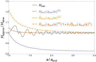
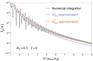
Figure 1: Left: approximations of the Hubble rate given by eqs. (128) and (131) for the potential eq. (141). Right: approximations of the spectrum given by eqs. (129) and (139).

As an example, consider the potential

$$V(\phi)=M^{4}\left(1-\left(\frac{\phi}{v_{\phi}}\right)^{6}\right)^{2},$$ (141)

with $v_{\phi}=M_{P}/2$. The relevant parameters are

$$m_{\phi} =30.41H_{\mathrm{end}} \tilde{Q}_{\mathrm{end}} =4.875\times 10^{-3}$$ (142)

$$\alpha_{3} =5 \alpha_{4} =155/6$$ (143)

$$\alpha_{5} =260/3 \alpha_{6} =1844/9$$ (144)

$$h_{1} =-55/2 h_{2} =-119973/128$$ (145)

where the large numbers stem partly from the large $M_{p}/m_{\phi}$ ratio (see e.g. eq. (269) and the comment below (271) for further explanation). When the inflaton potential is quadratic, the Hubble rate has the time behavior of eq. (128). For general potentials, the Hubble rate is more accurately modeled as eq. (131), with the leading order $u^{-3/2}$ term dominating at late times. The ratio of these two estimates will deviate from unity for non-quadratic potentials, and this will change the magnitude of predicted spectrum and number density. For the potential eq. (141), this ratio is

$$\frac{\tilde{H}_{\mathrm{end}}^{3}}{H_{\mathrm{end}}^{3}}=1.843,$$ (146)

which deviates significantly from unity. The relative corrections to the $u^{-3/2}$ dominant contribution are

$$h_{1}\tilde{Q}_{\mathrm{end}} =-0.134\qquad\text{and}\qquad\frac{3}{5}\left(h_{1}^{2}+h_{2}\right)\tilde{Q}_{\mathrm{end}}^{2}=-2.58\times 10^{-3}.$$ (147)

Overall, the predictions given by eqs. (130) and (139) differ by a factor of around 1.6 for this example. As shown in figure 1, numerical results demonstrate this for the example potential eq. (141), with eq. (136) being a better numerical fit of the spectrum than eq. (129) at large $k$.

IX Comparison of different computational approaches

In this section, we compare some different approaches to computing the super-Hubble mass scale particle production. The second main result of this paper presented in section IX.2 is to note the $O(m_{\phi}/H)$ (which can easily be a factor of 100) enhancement in numerical integration efficiency is achieved for a formulation obtained by subtracting out the slowly varying component of $H$. All of our numerical illustrations will be done with a prototype inflationary model presented in subsection IX.1. In subsection IX.3, we compare the particle production results of the Gaussian spectral model of ref. [44] with a generalized Gaussian spectral model based on an adiabatic invariant and an analogous time-model of V. In subsection IX.4, we illustrate the time model in the context of potentials where the maximum displacement from the minimum of the potential is asymmetric on two sides of the minimum.

IX.1 Inflationary model used for illustration

As a prototype of an inflaton potential for low-scale inflation, we test the time model developed in this paper by considering the hilltop model :

$$V(\phi)=M^{4}\left(1-\left(\frac{\phi}{v_{\phi}}\right)^{n}\right)^{2},$$ (148)

where $n>2$ is an integer and $v_{\phi}>0$ is the vacuum expectation value of the inflaton at the minimum of its potential [64, 65, 31, 66, 67]. The mass of the inflaton near the minimum is

$$m_{\phi}=n\sqrt{2}M^{2}/v_{\phi}\,,$$ (149)

and there is an effective cubic interaction of field displacements from the minimum (as well as higher order interactions). The Hubble expansion rate at the end of inflation is estimated as $H_{\mathrm{end}}\simeq\left(\sqrt{3}M_{P}\right)^{-1}M^{2}$. By calculating the large-scale curvature perturbations, the scalar spectral index and the tensor-to-scalar ratio is found to be

$$n_{s}=1-\frac{2}{N}\frac{n-1}{n-2},\qquad r=\frac{16n}{N(n-2)}\left[\frac{1}{2Nn(n-2)}\frac{v_{\phi}^{2}}{M_{P}^{2}}\right]^{\frac{n}{n-2}},$$ (150)

where the e-folding number $N$ of the CMB lies between 50 and 60 [68]. As observed by the Planck satellite, the overall normalization of the curvature perturbation implies

$$P_{\zeta}\simeq\frac{M^{4}}{12\pi^{2}}\left[\frac{2n(N(n-2))^{n-1}}{v_{\phi}^{n}M_{P}^{n-4}}\right]^{\frac{2}{n-2}}\simeq 2.2\times 10^{-9},$$ (151)

which relates $M$ and $v_{\phi}$. Hence there is one free parameter left, which can be taken as $v_{\phi}$ [64].

The measured range of the spectral index ($n_{s}=0.968(6)$ at 1$\sigma$ level [69]) can be made consistent with $n\geq 6$ [64]. We take $n=6$ in the potential eq. (148) and $v_{\phi}=0.5M_{P}$ to compare to the numerical results of ref. [8]. This is a somewhat tuned model that could be destabilized by loop generated Planck suppressed operators, but it serves as an algebraically simple demonstration of the adiabatic invariant formalism. It is interesting that the cosmological data driven phenomenology favoring $n\geq 6$ also enforces $m_{\phi}/H\gg 1$ since

$$\frac{m_{\phi}}{H_{\mathrm{end}}}\approx\frac{n\sqrt{2}M^{2}/v_{\phi}}{\sqrt{M^{4}/(3M_{P}^{2})}}=2n\sqrt{6},$$ (152)

which is equivalent to the condition $m_{\phi}\approx 30H_{\mathrm{end}}$ with $n=6$. As we saw in eqs. (143) and (144), the expansion in non-quadratic parameters $\alpha_{n}\propto\partial_{\phi}^{n}V$ defined in eq. (233) allows us to capture many different models [15, 70, 71] even though we focused for numerical illustrations on the model of eq. (148).

IX.2 Exact versus fast component numerical integration

In this section, we will summarize our numerical procedure to compute $\beta_{k}$ using the brute force exact integration eq. (8) and the fast only component integration eq. (9). We will then discuss figures that illustrate the differences between these methods, and explain observed features.

Both methods first required solving for the solution $\phi_{\mathrm{ode}}(t)$ to the inflaton equation of motion, given by the non-linear ordinary differential equation

$$\ddot{\phi}_{\mathrm{ode}}+3\sqrt{\frac{\frac{1}{2}\dot{\phi}_{\mathrm{ode}}^{2}+V(\phi_{\mathrm{ode}})}{3M_{P}^{2}}}\dot{\phi}_{\mathrm{ode}}+V^{\prime}(\phi_{\mathrm{ode}})=0,$$ (153)

where we assumed a background homogeneous inflaton field that dominates the energy density. Here the initial conditions and parameters were chosen such that at least $N\approx 55$ e-folds in the scale factor occurred before the end of inflation. We used the initial conditions $\phi(t_{i})=0.17\phi_{\mathrm{end}}$ and $\dot{\phi}(t_{i})=0$, and found that $t_{i}-t_{\mathrm{end}}\approx-63H_{\mathrm{end}}^{-1}$. It was found that the relevant portions of the ODE solution were nearly independent of the slow roll initial conditions.

The time $t_{\mathrm{end}}$ when the quasi-dS era ends is given by the solution to

$$\phi_{\mathrm{ode}}(t_{\mathrm{end}})=\phi_{\mathrm{end}}\equiv v_{\phi}\left(\frac{v_{\phi}}{\sqrt{2}nM_{P}}\right)^{1/(n-1)},$$ (154)

following the criterion used in ref. [8]. For the sake of convenience, we shifted time such that $t_{\mathrm{end}}=0$. We also set our time scale such that $M=5297H_{\mathrm{end}}$ and $M_{P}=1.565\times 10^{7}H_{\mathrm{end}}$, where we have defined

$$H_{\mathrm{end}}\equiv\sqrt{\frac{V(\phi_{\mathrm{end}})}{3M_{P}^{2}}},$$ (155)

which is approximately the usual Hubble expansion rate at the end of inflation.

The Hubble rate and Ricci scalar were determined by the Einstein equations $3M_{P}^{2}H_{\mathrm{ode}}^{2}=$ $\frac{1}{2}\dot{\phi}_{\mathrm{ode}}^{2}+V(\phi_{\mathrm{ode}})$, and $M_{P}^{2}R_{\mathrm{ode}}=\dot{\phi}_{\mathrm{ode}}^{2}-4V(\phi_{\mathrm{ode}})$, respectively. The scalar factor was then computed by solving $\dot{a}_{\mathrm{ode}}=H_{\mathrm{ode}}a_{\mathrm{ode}}$. With these quantities in hand, we evaluated the exact $\beta_{k}$ integration as

$$\beta_{k}^{(\mathrm{exact})}(t_{f}) =\frac{1}{2}\int_{t_{i}}^{t_{f}}dt\frac{H_{\mathrm{ode}}(t)m_{\chi}^{2}+\frac{1}{12}(1-6\xi)\left(\dot{R}_{\mathrm{ode}}(t)+2H_{\mathrm{ode}}(t)R_{\mathrm{ode}}(t)\right)}{\frac{k^{2}}{a_{\mathrm{ode}}^{2}(t)}+m_{\chi}^{2}+\frac{1}{6}(1-6\xi)R_{\mathrm{ode}}(t)}e^{-2i\Phi_{k}(t)}$$ (156)

$$\Phi_{k}(t) \equiv\int_{t_{i}}^{t}dt^{\prime}\sqrt{\frac{k^{2}}{a_{\mathrm{ode}}^{2}(t^{\prime})}+m_{\chi}^{2}+\frac{1}{6}(1-6\xi)R_{\mathrm{ode}}(t^{\prime})},$$ (157)

where $t_{i}$ was chosen sufficiently in the past compared to $t_{\mathrm{end}}$ to approximate the adiabatic initial conditions of the Bunch-Davies vacuum. In our computations, we chose $H_{\mathrm{end}}(t_{i}-t_{\mathrm{end}})=-5$.

To obtain the necessary components for the fast only integration, we solved the adiabatic invariant equation to obtain the slow time behavior of the Hubble expansion parameter. We first defined

$$J(V_{m})=2\int d\phi\Theta\left(V_{m}-V(\phi)\right)\sqrt{2V_{m}-2V(\phi)},$$ (158)

and computed it for various values of $V_{m}$ starting with $V(\phi_{\mathrm{end}})$ and proceeding to smaller values as needed. The step function ensured that finding the turning points was numerically unnecessary, and the smooth monotonic nature of the integration ensured that only a few sampling points of $V_{m}$ were needed to obtain a good interpolation.

The monotonic nature of $J(V_{m})$ also guarantees the existence of its inverse. The adiabatic invariant equation $Q=a_{\mathrm{slow}}^{3}J(V_{m})$ can then be written as

$$V_{m}(a_{\mathrm{slow}})=\mathrm{inverse\,of\,}J\left(Qa_{\mathrm{slow}}^{-3}\right),$$ (159)

which determines $V_{m}$ in terms of $a_{\mathrm{slow}}$. We computed the adiabatic invariant using the initial conditions as $Q=a_{\mathrm{end}}^{3}J\left(V(\phi_{\mathrm{end}})\right)$. The time dependence of $a_{\mathrm{slow}}$ was then obtained by integrating

$$\dot{a}_{\mathrm{slow}}=a_{\mathrm{slow}}\sqrt{\frac{V_{m}(a_{\mathrm{slow}})}{3M_{P}^{2}}},$$ (160)

with the initial condition being $a_{\mathrm{slow}}(t_{\mathrm{end}})=a_{\mathrm{end}}$. For convenience, we chose for our numerical work the normalization $a_{\mathrm{end}}=1$.

With $a_{\mathrm{slow}}(t)$ in hand, we arrived at the desired quantities

$$H_{\mathrm{slow}}(t)\equiv\sqrt{\frac{V_{m}(a_{\mathrm{slow}}(t))}{3M_{P}^{2}}},\quad\text{and}\quad H_{\mathrm{fast}}(t)\equiv H_{\mathrm{ode}}(t)-H_{\mathrm{slow}}(t),$$ (161)

where $H_{\mathrm{fast}}$ is defined to be zero before $t_{\mathrm{end}}$. One can compute other slowly varying quantities by taking $\langle\frac{1}{2}\dot{\phi}^{2}\rangle_{\mathrm{slow}}=\langle V(\phi)\rangle_{\mathrm{slow}}\approx\frac{1}{2}V_{m}(a_{\mathrm{slow}}(t))$. For example, $\rho_{\mathrm{slow}}=V_{m}$ and $R_{\mathrm{slow}}=-V_{m}/M_{P}^{2}$. However, only $H_{\mathrm{slow}}$ was necessary for our purposes here as $\dot{R}_{\mathrm{ode}}$ is dominated by its oscillatory components.

The fast only integration refers to subtracting out the slow components and sub-leading contributions, such as assuming that $\dot{R}\gg HR$ and $m_{\chi}^{2}\gg R$, as indicated by eq. (9). We also assumed $\dot{R}_{\mathrm{slow}}\ll\dot{R}_{\mathrm{fast}}$ and kept $R_{\mathrm{ode}}$ for the sake of computational simplicity and accuracy. For similar reasons, we avoided replacing $a_{\mathrm{ode}}$ with $a_{\mathrm{slow}}$. In summary, we evaluated

$$\beta_{k}^{(\mathrm{fast})}(t_{f}) =\frac{1}{2}\int_{t_{\mathrm{end}}}^{t_{f}}dt\left(H_{\text{fast}}(t)+\frac{1}{12}\left(1-6\xi\right)\frac{\dot{R}_{\mathrm{ode}}(t)}{m_{\chi}^{2}}\right)\frac{m_{\chi}^{2}}{E_{k}^{2}(t)}e^{-2i\int_{t_{\text{end}}}^{t}E_{k}(t^{\prime})dt^{\prime}},$$ (162)

where $E_{k}(t)=\sqrt{k^{2}/a_{\mathrm{ode}}^{2}(t)+m_{\chi}^{2}}$. The integration time $t_{f}$ should be chosen long enough such that the dominant resonance occurs for a given $k$ mode i.e. $t_{f}>\bar{v}_{k}$, where $\bar{v}_{k}$ is defined in eq. (125). This is particularly important for particle mass $m_{\chi}$ close to the $m_{\phi}$ threshold. The scale factor at resonance is $a(\bar{v}_{k})\approx k/\sqrt{m_{\phi}^{2}-m_{\chi}^{2}}$, and therefore $\bar{v}_{k}\rightarrow\infty$ as $m_{\chi}\rightarrow m_{\phi}$. In practice, one uses a cutoff $k_{c}$ for the wave-vector integration of the number density. The relative error incurred in the number density can be estimated to be

$$\left(\frac{k_{c}/a_{\mathrm{end}}}{\sqrt{m_{\phi}^{2}-m_{\chi}^{2}}}\right)^{-3/2},$$ (163)

as implied by eq. (130).

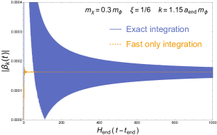
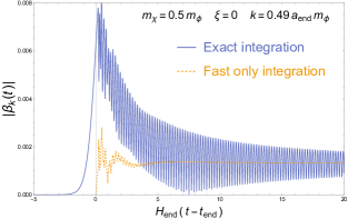
Figure 2: The exact (slow+fast) vs fast only integrations for computing $\beta_{k}(t)$, given by eqs. (156) and (162), respectively, are compared for the inflationary model of eq. (148). Although both methods tend towards nearly identical asymptotic values, the fast integration converges 3 orders of magnitude faster in integration time than the exact integration. The long convergence time of the latter is due to the slowly varying component in eq. (8), which damps down only as $t^{-1}$ for large times. On the right, we see that the exact integration is sensitive to the initial conditions before the end of inflation, while the fast integration is not. Starting the exact integration at $t_{\text{end}}$ would lead to a large deviation in the asymptotic limit, which is due to the adiabatic condition not being satisfied at that time.

Figure 2 illustrates the efficiency advantage of fast integration formulation of eq. (162) over the exact integration formulation of eq. (8). For this illustration, the parameters were chosen such that the $2\rightarrow 2$ resonance at time (see eq. (122)) in the $m_{\phi}/H_{\mathrm{end}}\approx 30$ model of section IX.1 is at $t$ satisfying

$$\frac{H_{\mathrm{end}}t_{\mathrm{end}}}{H_{\mathrm{end}}t}\approx\left(\frac{a_{\text{end}}}{a_{\mathrm{slow}}(t)}\right)^{3/2}\sim O(1),$$ (164)

which explains the spike in the dashed curve at near unity time. The fast integration formulation of eq. (162) occurs because the integration over the sinc function in eq. (121) converges on a time scale

$$\Delta t\approx\frac{14}{m_{\phi}}\approx\frac{14}{30}H_{\mathrm{end}}^{-1},$$ (165)

as given by  eq. (119).

The comparatively slow convergence of the “exact” numerical integration stems from

$$\beta_{k}(t)=\frac{1}{2}\int^{t}dt^{\prime}\frac{m_{\chi}^{2}H(t^{\prime})}{k^{2}/a^{2}+m_{\chi}^{2}}e^{-2i\int_{-\infty}^{t^{\prime}}dt^{\prime\prime}\frac{\omega_{k}(t^{\prime\prime})}{a(t^{\prime\prime})}},$$ (166)

which has a fluctuation amplitude $\Delta\beta_{k}$ scaling as $t^{-1}$ if $k/a\ll 1$ after the resonance is reached. This requires an integration time $t$ of

$$H_{\mathrm{end}}t\sim 10^{-1}|\Delta\beta|^{-1}$$ (167)

for $|\Delta\beta|$ is the accuracy of the amplitude that is desired. For figure 2, the final $|\beta_{k}|$ is $O(10^{-4})$, which means we require an accuracy of $|\Delta\beta|\sim|\beta_{k}|\sim 10^{-4}$. This gives a convergence time of

$$H_{\mathrm{end}}t\gtrsim 10^{3}.$$ (168)

for the brute force numerical integration (“exact integration”). As shown by eq. (167), the advantage of the fast only integration method increases for small $|\beta_{k}|$ which is typical for the scenarios of physical interest.

Figure 2 illustrates another advantage of the fast only integration technique over the exact integration for a mode slightly off resonance at the initial time $t_{\mathrm{end}}$. The exact integration is more sensitive to satisfying the adiabatic vacuum condition during the quasi-dS era because imposing the standard adiabatic vacuum condition at a non-adiabatic time of $t_{\mathrm{end}}$ is apparently an excited state which contains a sizable amount late time high frequency particle modes. On the other hand the fast only integration started at $t_{\mathrm{end}}$ has by construction subtracted out the leading nonadiabaticity governed by $O(H_{\mathrm{end}})$ dynamical scales, giving rise to an apparently acceptable level of consistency with the implicitly assumed adiabaticity (with respect to high frequency modes) at $t_{\mathrm{end}}$.

To put this another way, assuming an adiabatic boundary condition at a nonadiabatic time with an adiabaticity violating scale of $O(H_{\mathrm{end}})$ is equivalent to assuming the extra presence of late-time high frequency (i.e. $\omega_{k}/a_{\mathrm{end}}\gg H_{\mathrm{end}}$) modes, even though naively $O(H_{\mathrm{end}})$ nonadiabaticity should not contain any high frequency components. This somewhat surprising result may be due to the fact that imposing the adiabatic vacuum boundary condition at a nonadiabatic time $t_{\mathrm{end}}$ implicitly contains a step function in time with a non-negligible amplitude, which necessarily includes non-negligible high frequency components.

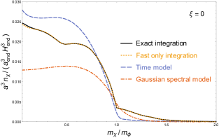
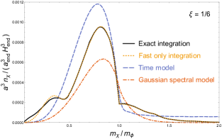
Figure 3: Different approximations of the number density $a^{3}n_{\chi}$ as a function of the mass $m_{\chi}$ are compared. In both the exact and fast only integrations, there is a clear threshold behavior at $m_{\chi}=m_{\phi}$. For $m_{\chi}<m_{\phi}$, there is an approximate factor of $2$ difference between the time model and the Gaussian spectral model, as noted below eq. (130). The “Time model” here refers to the symmetric time model of eq. (175). The “Gaussian spectral model” is defined according to eq. (171).

The produced $\chi$ number density as a function of $m_{\chi}$ is shown using various approximations in figure 3. The “Exact integration” and “Fast only integration” use eqs. (156) and (162), respectively, along with eq. (7). The figure clearly shows that the number density reaches a significant threshold at $m_{\chi}=m_{\phi}$. This is due to the $\delta\phi\delta\phi\rightarrow\chi\chi$ resonance becoming kinematically suppressed. A similar suppression of the $\delta\phi\rightarrow\chi\chi$ resonance causes the slope change around the $m_{\chi}=\frac{1}{2}m_{\phi}$ threshold. The largest deviation between the fast only and exact integrations occurs at low $m_{\chi}$, where the assumption of $m_{\chi}^{2}\gg R$ made in eq, (10) becomes less accurate.

IX.3 Time model versus Gaussian model

In this subsection, we generalize the Gaussian spectral model of ref. [44] and compare its computational accuracy with that of the symmetric time model of eq. (121). In both models, we compute the spectrum using the Boltzmann equation approximation form of eq. (47):

$$f_{\chi}(k,t)=\int_{t_{\mathrm{end}}}^{t}\frac{dv}{\Delta t(v)}\left|\tilde{b}_{k}(v)\right|^{2},$$ (169)

where $\Delta t(v)$ and $\tilde{b}_{k}(v)$ will be defined differently based on the model: i.e. $\{\Delta t\rightarrow\Delta t^{(\mathrm{GS})},\tilde{b}_{k}\rightarrow\tilde{b}_{k}^{(\mathrm{GS})}\}$ or $\{\Delta t\rightarrow\Delta t^{(\mathrm{TM})},\tilde{b}_{k}\rightarrow\tilde{b}_{k}^{(\mathrm{TM})}(v)\}$.

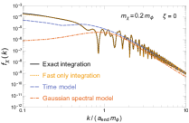
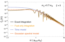
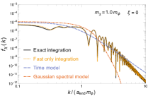
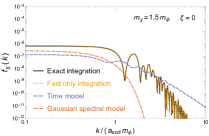
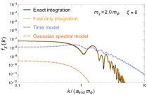
Figure 4: This figure compares the produced particle spectrum computed using the Bogoliubov integration eq. (156), fast only integration eq. (162), Gaussian spectral model eq. (171), and the time model eq. (175). Note that for $m_{\chi}<m_{\phi}$, and $k>m_{\phi}a_{\mathrm{end}}$, the time model and exact integration match while the spectral model differs from both by a factor of 2. The spectrum in this regime scales like $k^{-9/2}$, which appears as linear behavior on this log-log plot.

As discussed in section II, the Gaussian model had several shortcomings partly because of the ambiguities associated with mapping to Boltzmann equations as well as not having a long time understanding of oscillating field amplitudes. The Gaussian spectral model with the adiabatic invariant evolved fields resolving these deficiencies is defined by generalizing the Gaussian model of ref. [44] as

$$\Delta t^{(\mathrm{GS})}(v) =\frac{\sqrt{2\pi}}{\sigma(v)},$$ (170)

$$\tilde{b}_{k}^{(\mathrm{GS})}(v) \approx\frac{\pi}{8i}\left(\frac{\Delta\phi(v)}{M_{P}}\right)^{2}\left(\left(1-6\xi\right)E_{k}(v)+\frac{m_{\chi}^{2}}{2E_{k}(v)}\right)\frac{1}{\sqrt{4\pi\sigma^{2}(v)}}e^{-\left(E_{k}(v)-\omega_{*}(v)\right)^{2}/\sigma^{2}(v)},$$ (171)

$$\omega_{*}(v) =\frac{2\pi}{\oint_{C}d\phi/\sqrt{2V_{m}(v)-2V(\phi)}}$$ (172)

where the width $\sigma(v)$ is defined as

$$\sigma^{2}(v)=\left|\frac{V^{\prime}\left(\phi_{C,+}(v)\right)-V^{\prime}\left(\phi_{C,-}(v)\right)}{\phi_{C,+}(v)-\phi_{C,-}(v)}-\omega_{*}^{2}(v)\right|+\epsilon,$$ (173)

with $\epsilon$ as a small positive parameter to ensure computational convergence. This model still has the limitation that the spectrum has a limited shape, but it will be able to reproduce the high $k$ part of the spectrum as can be seen in figure 4. This analytic fit to the high $k$ part of the spectrum was used as the primary guidance in the generalization of the Gaussian model.

In the time model, we have instead from eq. (121) the expressions

$$\Delta t^{(\mathrm{TM})}(v) =\sqrt{\frac{2\pi}{m_{\phi}H_{\text{slow}}(v)}},$$ (174)

$$\tilde{b}_{k}^{(\mathrm{TM})}(v) =\frac{3\pi}{4i}\frac{H_{\text{slow}}^{2}(v)}{\omega_{*}(v)}\left(\frac{\left(1-6\xi\right)\omega_{*}^{2}(v)+\frac{1}{2}m_{\chi}^{2}}{E_{k}^{2}(v)}\right)\frac{\Delta t(v)}{2\pi}\text{sinc}\left[\Delta t(v)\left(E_{k}(v)-\omega_{*}(v)\right)\right],$$ (175)

$$\omega_{*}(v) =\sqrt{\frac{2V_{m}(v)}{[\Delta\phi(v)]^{2}}},$$ (176)

which are similar to eq. (171) in having a peaked function, but different in how fast that peaked function falls off with $E_{k}-\omega_{*}$. The $\mathrm{sinc}$ function falls off much slower and has multiple peaks. Furthermore, the prefactors dependent on the non-minimal coupling parameter $\xi$ are different and can become significant for large $\omega_{*}/E_{k}\sim m_{\phi}/m_{\chi}$ applicable for small $k/(a_{\mathrm{end}}m_{\phi})$. These features can be seen in figure 4.

Shown in figure 3 is also the integrated number density of the “Time model” (eq. (175)) and the “Gaussian spectral model” (eq. (171)). The “Time model” plot does not fall off with large $m_{\chi}/m_{\phi}$ because eq. (175) grows as $m_{\chi}^{2}$ and therefore the rate is boosted by an $m_{\chi}^{4}$ factor. Even though the minimally coupled case plot seems to indicate that the large $m_{\chi}/m_{\phi}$ region has a vanishing asymptote, this is an illusion associated with the vertical resolution of the figure. This mismatch between the “Time model” approximation and the better approximation of the “Fast only integration” is due to the loss of validity in the kinematic region in which eq. (2) does not have a solution (e.g. see eq.(118)).

In fact, for the symmetric time model, one can interpret the nonzero $a^{3}n_{\chi}$ for the $m_{\chi}>m_{\phi}$ parametric region as an error on the particle production computation for any finite $v$. Using eqs. (7),  (47) and (175), we can estimate this error as

$$\Delta\left(a^{3}(t)n_{\chi}(t)\right)\sim\left.\frac{9}{512\pi^{2}}m_{\chi}\int_{t_{\mathrm{end}}}^{t}\frac{dv}{\Delta t(v)}\left(\frac{H_{\text{slow}}^{2}(v)}{m_{\phi}}\right)^{2}a_{\mathrm{slow}}^{3}\int_{0}^{\infty}dw\frac{w^{2}}{\left(w^{2}+1\right)^{3}}\right|_{m_{\chi}=m_{\phi}}$$ (177)

which with

$$H_{\mathrm{slow}}(v)\approx\frac{H_{i}}{1+\frac{3}{2}H_{i}(v-t_{i})}$$ (178)

evaluates to

$$\Delta\left(\frac{a^{3}}{a_{i}^{3}}n_{\chi}\right)\sim\frac{1}{2048\sqrt{2}\pi^{3/2}}\frac{H_{i}^{7/2}}{m_{\phi}^{1/2}}$$ (179)

which is suppressed by $\sqrt{H_{i}/m_{\phi}}$ and the small prefactor. The Gaussian model in contrast has an exponentially suppressed error as $m_{\chi}/m_{\phi}$ becomes larger than unity.

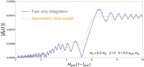
Figure 5: The Bogoliubov coefficient approximation results are compared for the asymmetric time model with the fast integration method. There are two spikes in the rate corresponding to the $\delta\phi\delta\phi\delta\phi\rightarrow\chi\chi$ and $\delta\phi\delta\phi\rightarrow\chi\chi$ resonances. In the case of the time model, $\left|\beta_{k}(t)\right|$ was obtained by taking the square root of $f_{\chi}(k,t)$, which was computed via eqs. (169), (180), and (181).

IX.4 Asymmetric time model

The time model in subsection IX.3 did not account for the $\delta\phi\delta\phi\delta\phi\rightarrow\chi\chi$ and $\delta\phi\rightarrow\chi\chi$ scattering. Using eq. (104), we can make the substitution $\{\Delta t\rightarrow\Delta t^{\mathrm{ASTM}},\tilde{b}_{k}\rightarrow\tilde{b}_{k}^{\mathrm{ASTM}}\}$ in eq. (169) where

$$\Delta t^{\mathrm{ASTM}} =\sqrt{\frac{2\pi}{m_{\phi}H_{\text{slow}}}},$$ (180)

$$\tilde{b}_{k}^{\mathrm{ASTM}} =\frac{A_{1}}{2}\frac{e^{i\left(\omega_{*}-2E_{k}\right)\Delta t}-1}{i(\omega_{*}-2E_{k})}+\frac{A_{2}}{2}\frac{e^{i\left(2\omega_{*}-2E_{k}\right)\Delta t}-1}{i(2\omega_{*}-2E_{k})}+\frac{A_{3}}{2}\frac{e^{i\left(3\omega_{*}-2E_{k}\right)\Delta t}-1}{i(3\omega_{*}-2E_{k})},$$ (181)

and $A_{n}$ are amplitudes given by eqs. (102), (100), and (101). Notice that because $\omega_{*}\approx m_{\phi}$ while $E_{k}$ redshifts, one can see from the denominators of eq. (181) that $\delta\phi\delta\phi\delta\phi\rightarrow\chi\chi$ amplitude $A_{3}$ will be reached first before the $\delta\phi\delta\phi\rightarrow\chi\chi$ amplitude as a function of time for $2m_{\chi}<3m_{\phi}$

The time evolution of the particle spectrum for an example parametric point is shown in figure 5. In the following argument, we will set $t_{\mathrm{end}}=0$ for convenience. Using the resonance condition $3\omega_{*}=2E_{k}$, we would predict a step in particle spectrum time evolution at

$$a(t_{*})=\frac{k}{\sqrt{\left(\frac{3}{2}\omega_{*}\right)^{2}-m_{\chi}^{2}}}\qquad\Rightarrow\qquad H_{\mathrm{end}}t_{*}\approx\frac{2}{3}\left[\left(\frac{k/(m_{\phi}a_{\mathrm{end}})}{\sqrt{9/4-m_{\chi}^{2}/m_{\phi}^{2}}}\right)^{3/2}-1\right],$$ (182)

which is consistent with the step feature in the figure near $H_{\mathrm{end}}t\approx 3$. The step at $H_{\mathrm{end}}t\approx 5.5$ is due to the dominant $2\omega_{*}=2E_{k}$ resonance.

X Summary

In this paper, we developed analytic and numerical techniques to compute the Bogoliubov coefficient $\beta_{k}$ more accurately and efficiently. Using the adiabatic invariant equation, we computed the slowly varying components of the $\beta_{k}$ integrand necessary to implement the fast-slow decomposition formalism of ref. [44]. In the process, a numerical integration technique was created that is O(1000) faster than a brute force computation.

To compute the particle production rate and number density, an approximation of the Boltzmann equation was presented, and a coarse graining time $\Delta t$ was introduced. We demonstrated that $\Delta t$ minimizes the error of this approximation at an intermediate scale between the inflaton mass and Hubble rate, and that the overall error is suppressed by powers of $H/m_{\phi}$. This simplified the integration by linearizing the phase of the Bogoliubov integrand, yielding a form reminiscent of a Fourier transform.

We derived a time model of inflaton dynamics and used it simplify the $\beta_{k}$ integrand to a form amenable to exact analytical integration. This was done using the adiabatic turning points to create an envelope of the oscillatory motion. A differential equation for the fast oscillatory phase was then obtained using approximate energy conservation. By treating the slowly varying components as constant, and using a perturbative expansion of the inflaton potential, the phase was obtained as a function of adiabatic invariants.

A closed form production rate proportional to a sine-cardinal function was derived, with a resonant peak when the inflaton oscillatory frequency $\omega_{*}$ equals the time derivative of the Bogoliubov phase $E_{k}$. We then integrated the production rate to obtain the spectrum and number density. For $m_{\chi}<m_{\phi}$ and large $k$, these results matched the exact Bogoliubov integration.

For $k>m_{\phi}a_{\mathrm{end}}$, the rate limits to the form of Fermi’s golden rule for the tree-level graviton-mediated process $\phi\phi\rightarrow\chi\chi$ in a frame where both inflatons are at rest. In this case, $\omega_{*}$ and $E_{k}$ can be interpreted as the energies of the $\phi$ and $\chi$ particles, respectively. The delta function in the production rate allowed an analytical evaluation of the time integral, which yielded simple closed form approximations of the spectrum and number density. These made O(1) corrections to the predictions of the Gaussian spectral model of ref. [44].

This formalism demonstrates a correspondence between the Bogoliubov and scattering methods of computing gravitational particle production. The predicted spectrum and number density are the same, up to factors of 2, as the results of papers that considered a gas of inflatons at rest undergoing gravitational annihilation [42, 41]. These factors of 2 are not currently understood, but we suspect that the inflaton gas must be treated as an appropriate coherent state in the scattering picture to obtain an exact correspondence.

The noisy behavior of the numerical spectrum as a function of $k$ (see for example numerical results of ref. [8] and figure 4 of the present work) remains unexplained and is a subject of ongoing research by our group. Preliminary results suggest this is due to quantum interference between different resonances of the Bogoliubov integral, and have interesting implications for the particle scattering method of computing gravitational particle production. It would also be of great interest to find cosmological observables that are sensitive to the details in the momentum spectrum of the gravitationally produced particles, which is one of the main results of this paper.

Appendix A Adiabatic invariant

Here we give a clarification of the adiabatic invariant construction presented in ref. [73]. In addition to the derivation of the conserved adiabatic invariant expression of eq. (207), the error incurred over a long time period $T/\epsilon$ (where $T$ is the period of fast periodic motion and $\epsilon$ is a small adiabaticity parameter) is explicitly evaluated in eq. (216) using eq. (208). We also compare it to the canonical transformation approach of ref. [74].

Consider an external influence on the system represented by the function $\lambda(t)$. The Hamiltonian of the system is denoted as $H(\vec{q},\vec{\pi},\lambda(t))$, where $\vec{\pi}$ is the conjugate momentum to $\vec{q}$. Suppose this function is slowly (adiabatically) changing such that

$$T\frac{d\lambda}{dt}+T^{2}\frac{d^{2}\lambda}{dt^{2}}+...\ll\lambda$$ (183)

on a time scale $T$. The energy $E(t)\equiv H(\vec{q}(t),\vec{\pi}(t),\lambda(t))$ is not conserved because of the time dependence of $\lambda(t)$. We write the time average of $dE/dt$ at time $v$ over a time period $T$ as

$$\left\langle\frac{dE(t)}{dt}\right\rangle_{v} =\left\langle\frac{d\lambda}{dt}\partial_{\lambda}H\right\rangle_{v}\approx\frac{1}{T}\left.\frac{d\lambda}{dt}\right|_{v}\int_{v}^{v+T}dt\,\partial_{\lambda}H(\vec{q}(t),\vec{\pi}(t),\lambda(v))+\Delta_{1}(v),$$ (184)

where the leading order error $\Delta_{1}$ is estimated as

$$\Delta_{1}(v) \equiv\frac{1}{T}\int_{v}^{v+T}dt(t-v)\left(\left.\frac{d^{2}\lambda}{dt^{2}}\right|_{v}\partial_{\lambda}H(\vec{q}(t),\vec{\pi}(t),\lambda(v))+\left(\left.\frac{d\lambda}{dt}\right|_{v}\right)^{2}\partial_{\lambda}^{2}H(\vec{q}(t),\vec{\pi}(t),\lambda(v))\right)$$ (185)

through a Taylor expansion.

Next, restrict to a 1-dimensional motion which becomes periodic in $t$ when $\lambda(t)$ becomes independent of $t$ as $\lambda(t)=\lambda(v)$. Define $\Pi(q,E,\lambda)$ to be the solution to

$$E=H\left(q,\Pi(q,E,\lambda),\lambda\right)$$ (186)

as an algebraic identity. Using this, we can define the time period to be

$$T(v) \equiv \int_{v}^{v+T}dt$$ (187)

$$\approx \oint_{C_{T}(v)}\frac{dq^{\prime}}{\partial_{\pi}H\left(q^{\prime},\Pi\left[q^{\prime},E(v),\lambda(v)\right],\lambda(v)\right)}\left(1+\Delta_{2}\right)$$ (188)

$$\Delta_{2} \equiv \frac{O\left([q(v+T)-q(v)]\left.\frac{dt}{dq}\right|_{v}\right)}{\oint_{C_{T}(v)}\frac{dq^{\prime}}{\partial_{\pi}H(q^{\prime},\Pi\left[q^{\prime},E(v),\lambda(v)\right],\lambda(v))}},$$ (189)

where $C_{T}(v)$ represents a chosen 1-dimensional path where $q_{C}(t)$ returns to itself periodically with $\lambda(t)=\lambda(v)$ fixed, i.e. $q_{C}(t)$ is a solution to the equation of motion with $\lambda(t)=\lambda(v)$.

From eq. (186), we conclude

$$\frac{dE}{d\lambda} =\partial_{\lambda}H\left(q,\Pi\left(q,E,\lambda\right),\lambda\right)+\partial_{\lambda}\Pi\left(q,E,\lambda\right)\partial_{\pi}H\left(q,\Pi\left(q,E,\lambda\right),\lambda\right)=0,$$ (190)

as $E$ and $\lambda$ are independent variables. One can use this to write

$$dt=-dq\frac{\partial_{\lambda}\Pi[q,E(t),\lambda(t)]}{\partial_{\lambda}H\left(q,\Pi\left(q,E(t),\lambda(t)\right),\lambda(t)\right)},$$ (191)

where we made use of $\dot{q}=\partial_{\pi}H\left(q,\Pi\left(q,E,\lambda\right),\lambda\right)$ just as in eq. (188). Since there are 2 values of $t$ for a given value of $q$ in the time interval $[v,v+T]$, we will call one branch of eq. (184) integral “branch 1” and the other “branch 2”. Putting eq. (191) into eq. (184) gives

$$\left\langle\frac{dE(t)}{dt}\right\rangle_{v} \approx\frac{-1}{T}\left.\frac{d\lambda}{dt}\right|_{v}\left[\int_{\mathrm{branch\,1}}dq^{\prime}+\int_{\mathrm{branch\,2}}dq^{\prime}\right]\partial_{\lambda}\Pi\left[q^{\prime},E(\tilde{t}(q^{\prime})),\lambda(\tilde{t}(q^{\prime}))\right]+\Delta_{1}(v),$$ (192)

where $\tilde{t}(q^{\prime})$ is the implicit solution of eq. (191) such that $\tilde{t}(q(t))=t$.

As the external parameter is fixed at $\lambda=\lambda(v)$ without time variation for which $q_{C}(t)$ is defined below eq. (189), a small error is incurred by putting in approximate solutions with $\lambda$ fixed. Therefore, we define the error $\Delta_{4}$ as

$$\partial_{\lambda}\Pi(q(t),E(t),\lambda(t))=\partial_{\lambda}\Pi(q_{C}(t),E(v),\lambda(v))\left(1+\Delta_{4}(t)\right),$$ (193)

where

$$\Delta_{4}(t)\equiv\frac{\partial_{\lambda}\Pi(q(t),E(t),\lambda(t))}{\partial_{\lambda}\Pi(q_{C}(t),E(v),\lambda(v))}-1$$ (194)

which is still a function of time. Putting this in to eq. (192) gives

$$\left\langle\frac{dE(t)}{dt}\right\rangle_{v} =-\frac{1}{T(v)}\left.\frac{d\lambda}{dt}\right|_{v}\oint_{C_{T}(v)}dq^{\prime}\partial_{\lambda}\Pi[q^{\prime},E(v),\lambda(v)]\left(1+\Delta_{4}(\tilde{t}(q^{\prime}))\right)+\Delta_{1}(v),$$ (195)

which implies

$$0 =T(v)\left(\left\langle\frac{dE(t)}{dt}\right\rangle_{v}-\Delta_{1}(v)\right)+\left.\frac{d\lambda}{dt}\right|_{v}\oint_{C_{T}(v)}dq^{\prime}\partial_{\lambda}\Pi[q^{\prime},E(v),\lambda(v)]\left(1+\Delta_{4}(\tilde{t}(q^{\prime}))\right)$$ (196)

$$=\oint_{C_{T}(v)}dq^{\prime}\left[\frac{\left(1+\Delta_{2}(q^{\prime},v)\right)\left(\left\langle\frac{dE(t)}{dt}\right\rangle_{v}-\Delta_{1}(v)\right)}{\partial_{\pi}H\left(q^{\prime},\Pi\left[q^{\prime},E(v),\lambda(v)\right],\lambda(v)\right)}+\left.\frac{d\lambda}{dt}\right|_{v}\partial_{\lambda}\Pi[q^{\prime},E(v),\lambda(v)]\left(1+\Delta_{4}(\tilde{t}(q^{\prime}))\right)\right],$$ (197)

where we replaced $T(v)$ in the second line using eq. (187). Taking a derivative of eq. (186) with respect to $E$ yields

$$1=\partial_{E}\Pi\left(q,E,\lambda\right)\partial_{\pi}H\left(q,\Pi[q,E,\lambda],\lambda\right).$$ (198)

Combining this with eq. (197) results in

$$0=\oint_{C_{T}(v)}dq^{\prime}\left[\frac{\left(1+\Delta_{2}(q^{\prime},v)\right)\left(\left\langle\frac{dE(t)}{dt}\right\rangle_{v}-\Delta_{1}(v)\right)}{1/\partial_{E}\Pi\left(q^{\prime},E(v),\lambda(v)\right)}+\left.\frac{d\lambda}{dt}\right|_{v}\partial_{\lambda}\Pi\left(q^{\prime},E(v),\lambda(v)\right)\left(1+\Delta_{4}(\tilde{t}(q^{\prime}))\right)\right],$$ (199)

which almost brings us to the desired result after neglecting the $\Delta_{n}$ errors.

Given that $v$-dependent quantities do not depend on $t$, we expand the time-averaging in eq. (199) to the entire integral as

$$0=\left\langle\oint_{C_{T}(v)}dq^{\prime}\left[\frac{\left(1+\Delta_{2}(q^{\prime},v)\right)\left(\frac{dE(t)}{dt}-\Delta_{1}(v)\right)}{1/\partial_{E}\Pi\left(q^{\prime},E(v),\lambda(v)\right)}+\left.\frac{d\lambda}{dt}\right|_{v}\partial_{\lambda}\Pi\left(q^{\prime},E(v),\lambda(v)\right)\left(1+\Delta_{4}(\tilde{t}(q^{\prime}))\right)\right]\right\rangle_{v}$$ (200)

such that there is now a simple motivation to approximate judicious objects inside the more inclusive time average as a function of $t$. Taylor expanding $v$ dependent quantities $E(v)$ and $\lambda(v)$ about the point $t$, the integrand becomes

$$0 =\left\langle\oint_{C_{T}(v)}dq^{\prime}\left[\frac{\left(1+\Delta_{2}(q^{\prime},v)\right)\left(\left.\frac{dE}{dt}\right|_{t}-\Delta_{1}(v)\right)}{1/\partial_{E}\Pi\left(q^{\prime},E(t)-(t-v)\left.\frac{dE}{dt}\right|_{v},\lambda(t)-(t-v)\left.\frac{d\lambda}{dt}\right|_{v}\right)}+\left(\left.\frac{d\lambda}{dt}\right|_{t}-(t-v)\left.\frac{d^{2}\lambda}{dt}\right|_{v}\right)\right.\right.$$

$$\left.\left.\times\partial_{\lambda}\Pi\left(q^{\prime},E(t)-(t-v)\left.\frac{dE}{dt}\right|_{v},\lambda(t)-(t-v)\left.\frac{d\lambda}{dt}\right|_{v}\right)\left(1+\Delta_{4}(\tilde{t}(q^{\prime}))\right)\right]\right\rangle_{v},$$ (201)

and the function $\Pi$ can be expanded further as

$$\partial_{E}\Pi\left(q^{\prime},E(t)-(t-v)\left.\frac{dE}{dt}\right|_{v},\lambda(t)-(t-v)\left.\frac{d\lambda}{dt}\right|_{v}\right)$$

$$=\partial_{E}\Pi\left(q,E(t),\lambda(t)\right)-(t-v)\left(\left.\frac{dE}{dt}\right|_{t}\partial_{E}^{2}\Pi\left(q,\lambda(t),E(t)\right)+\left.\frac{d\lambda}{dt}\right|_{t}\partial_{\lambda}\partial_{E}\Pi\left(q,\lambda(t),E(t)\right)\right)+\dots,$$ (202)

$$\partial_{\lambda}\Pi\left(q^{\prime},E(t)-(t-v)\frac{dE}{dt}|_{t},\lambda(t)-(t-v)\frac{d\lambda}{dt}|_{t}\right)$$

$$=\partial_{\lambda}\Pi\left(q,E(t),\lambda(t)\right)-(t-v)\left(\left.\frac{dE}{dt}\right|_{t}\partial_{E}\partial_{\lambda}\Pi\left(q,\lambda(t),E(t)\right)+\left.\frac{d\lambda}{dt}\right|_{t}\partial_{\lambda}^{2}\Pi\left(q,\lambda(t),E(t)\right)\right)+\dots,$$ (203)

to obtain more small error quantities. We therefore define

$$\Delta_{3}(q,t,v) \equiv-(t-v)\left[\left(\left.\frac{dE}{dt}\right|_{t}\right)^{2}\partial_{E}^{2}\Pi\left(q,\lambda(t),E(t)\right)+2\left.\frac{dE}{dt}\right|_{t}\left.\frac{d\lambda}{dt}\right|_{t}\partial_{E}\partial_{\lambda}\Pi\left(q,\lambda(t),E(t)\right)\right.$$

$$\left.+\left(\left.\frac{d\lambda}{dt}\right|_{t}\right)^{2}\partial_{\lambda}^{2}\Pi\left(q,\lambda(t),E(t)\right)+\left.\frac{d^{2}\lambda}{dt^{2}}\right|_{v}\partial_{\lambda}\Pi\left(q,E(t),\lambda(t)\right)\right]$$ (204)

$$=O\left(\left(\frac{dE}{dt}\right)^{2},\frac{dE}{dt}\frac{d\lambda}{dt},\left(\frac{d\lambda}{dt}\right)^{2},\frac{d^{2}\lambda}{dt^{2}}\right),$$ (205)

as the error due to these last set of expansions.

Neglecting all $\Delta_{n}$, we find

$$0 =\left\langle\oint_{C_{T}(v)}dq^{\prime}\left[\left.\frac{dE}{dt}\right|_{t}\frac{\partial\Pi\left(q^{\prime},E(t),\lambda(t)\right)}{\partial E}+\left.\frac{d\lambda}{dt}\right|_{t}\frac{\partial\Pi[q^{\prime},E(t),\lambda(t)]}{\partial\lambda}\right]\right\rangle_{v},$$ (206)

or equivalently, the statement is that

$$\boxed{Q(t)\equiv\oint_{C_{T}(t)}dq^{\prime}\Pi\left(q^{\prime},E(t),\lambda(t)\right)}$$ (207)

is conserved when $\Delta_{n}$ are all neglected. To be more explicit, the identity is

$$\left\langle\dot{Q}\right\rangle_{v}=0$$

when errors $\Delta_{n}$ are neglected.

The correction to $Q(t)$ is

$$\Delta\left\langle\dot{Q}\right\rangle_{v} =\left\langle\oint_{C_{T}(v)}dq^{\prime}\left[\frac{\Delta_{2}(q^{\prime},v)\left.\frac{dE}{dt}\right|_{t}-\Delta_{1}(v)}{1/\partial_{E}\Pi\left(q^{\prime},E(t),\lambda(t)\right)}+\left.\frac{d\lambda}{dt}\right|_{t}\partial_{\lambda}\Pi\left(q^{\prime},E(t),\lambda(t)\right)\Delta_{4}(\tilde{t}(q^{\prime}))+\Delta_{3}(q^{\prime},t,v)\right]\right\rangle_{v}$$ (208)

to leading order in $\Delta_{n}$. Let us compute the change in $Q$ over a long time period over which $\lambda$ changes significantly, denoted as

$$\Delta t(v)\sim\frac{\lambda(v)}{\dot{\lambda}(v)}\equiv\frac{T(v)}{\epsilon(v)},$$ (209)

to leading order in $\epsilon\ll 1$. For a generic non-adiabatic-invariant quantity $\mathcal{O}_{\mathrm{NAI}}(t)$ that derives time dependence from $\lambda(t)$, the change over the long time period $\Delta t(v)$ is

$$\Delta\mathcal{O_{\mathrm{NAI}}}\sim\Delta t\left\langle\dot{\mathcal{O}}_{\mathrm{NAI}}\right\rangle_{v}\sim\mathcal{O}_{\mathrm{NAI}}$$ (210)

where the time average has been estimated as $\left\langle\dot{\mathcal{O}}_{\mathrm{NAI}}\right\rangle_{v}\sim\epsilon\mathcal{O}_{\mathrm{NAI}}/T(v)$ which exactly vanishes in the limit that $\lambda(t)$ becomes time independent. Note regardless of how small the time variation $\epsilon$ is, the change in $\mathcal{O}_{\mathrm{NAI}}$ over the long time period $\Delta t$ is large.

This is in contrast with the case of the adiabatic invariant for which the change is

$$\Delta Q =\Delta\left\langle\dot{Q}\right\rangle_{v}\Delta t\sim\left(\frac{O\left([q(v+T)-q(v)]\frac{dt}{dq}\right)}{T(v)}Q+QO(\epsilon)+\frac{T(v)}{\epsilon}\oint_{C_{T}(v)}dq^{\prime}\Delta_{3}(q^{\prime},T(v),v)\right)$$ (211)

where we have assumed, for example, $\dot{E}(t)\sim\dot{\lambda}(t)E/\lambda,$ $\ddot{\lambda}(t)/\lambda\sim O(\epsilon^{2})/T^{2}$, $Q\sim ET$, and $\partial_{\lambda}^{2}H(\vec{q},\vec{\pi},\lambda(v))\sim H/\lambda^{2}$, based on smoothness of these functions. Simplifying the large piece $\Delta_{3}$, we find

$$\frac{T(v)}{\epsilon}\oint_{C_{T}(v)}dq^{\prime}\Delta_{3}(q^{\prime},T(v),v) =QO(\epsilon)$$ (212)

and thus

$$\Delta Q\sim\left(\frac{O\left([q(v+T)-q(v)]\frac{dt}{dq}\right)}{T}+O(\epsilon)\right)Q$$ (213)

to be the variation in the adiabatic invariant charge $Q$ over a long time period $\Delta t\sim T/\epsilon$. This makes manifest the importance of the periodicity of $q$ motion. If the motion were not periodic, then we would conclude

$$\frac{O\left([q_{\mathrm{nonperiodic}}(v+T)-q_{\mathrm{nonperiodic}}(v)]\frac{dt}{dq_{\mathrm{nonperiodic}}}\right)}{T}\sim O(1)$$ (214)

leading to a result analogous to eq. (210). However, for periodic motion relevant to the adiabatic invariant construction, the first term in eq. (213) turns into

$$\frac{q(v+T)-q(v)}{\dot{q}}\sim\epsilon T,$$ (215)

resulting in

$$\frac{\Delta Q}{Q}\sim O(\epsilon),$$ (216)

which shows that $Q$ is conserved to leading order even on long time scales over which $\lambda$ changes.

This matches the more subtle analysis of ref. [74] where the key idea is to first derive the leading order approximation

$$\langle\dot{Q}\rangle_{T}=-\frac{\epsilon\dot{\lambda}(0)}{T}\int_{0}^{T}dt\frac{\partial}{\partial\Omega}\left(\left[\partial_{\lambda}\underline{F}_{1}(q(t),\Omega(t),\lambda(0))\right]_{q=q(\Omega,J,\lambda(0))}\right)$$ (217)

where $\underline{F}_{1}(q,\Omega,\lambda(0))$ is the generating function of the canonical transformation to a special set of variables: action angle variables $(\Omega,Q)$ for the time independent problem except with the constant parameter $\lambda(0)$ lifted to a function of time $\lambda(t)$. More explicitly, one first solves the phase space symplectic form preserving map $(q,p;\lambda(0))\leftrightarrow(\Omega,Q;\lambda(0))$ for the time independent problem, use this to find $p(q,\Omega;a(0))$ and $Q\left(q,\Omega;a(0)\right)$, make the replacement $a(0)\rightarrow a(t)$, and solve the differential equations

$$p(q,\Omega;a(t)) =\partial_{q}\underline{F_{1}}(q,\Omega,a(t)),$$ (218)

$$Q\left(q,\Omega;a(t)\right) =-\partial_{\Omega}\underline{F_{1}}(q,\Omega,a(t)),$$ (219)

to construct $\underline{F_{1}}(q,\Omega,a(t))$. Because of the action-angle variable choice, one can show that

$$\left[\partial_{\lambda}\underline{F}_{1}(q(t),\Omega(t),\lambda(0))\right]_{q=q(\Omega,J,\lambda(0))}\mbox{ and }\frac{\partial}{\partial\Omega}\left(\left[\partial_{\lambda}\underline{F}_{1}(q(t),\Omega(t),\lambda(0))\right]_{q=q(\Omega,J,\lambda(0))}\right),$$ (220)

are periodic with period $T$ such that eq. (217) vanishes.

Appendix B A perturbative expansion of the Hubble rate time dependence

In this section we will develop a formalism to estimate the time dependence of the adiabatic energy $V_{m}=V(\phi_{C,\pm})$ by using an expansion of the inflation potential from leading order behavior at its minimum. As the time dependence is given by the first few terms of this expansion, this formalism is broadly applicable to many models of inflation.

B.1 Integral equation

If we want to solve for $V_{m}$ as a function of scale factor $a_{\mathrm{slow}}$, we want to solve

$$\frac{Q}{2\sqrt{2}a_{\mathrm{slow}}^{3}V_{m}^{3/2}}=\int_{0}^{1}ds\frac{\sqrt{1-s}}{\left[-V^{\prime}(V_{<}^{-1}(sV_{m}))\right]}+\int_{0}^{1}ds\frac{\sqrt{1-s}}{V^{\prime}(V_{>}^{-1}(sV_{m}))}$$ (221)

obtained from eq. (20) for the potential at the oscillation maximum $V_{m}$ where

$$V_{>}^{-1}(V) \equiv V^{-1}(V)>\phi_{\mathrm{min}}$$ (222)

$$V_{<}^{-1}(V) \equiv V^{-1}(V)<\phi_{\mathrm{min}},$$ (223)

and we have shifted the potential such that minimum of the potential is at $V(\phi_{\mathrm{min}})=0$. For potentials $V(\phi)$ where the inverse function $V^{-1}(V)$ is simple enough for the integration to be executed in a closed form (such as monomial potentials), eq. (221) is useful. Since $Q$ is a constant, we can take ratios to write

$$\frac{a_{\mathrm{slow}}^{3}V_{m}^{3/2}}{a_{\mathrm{end}}^{3}V_{m}^{3/2}|_{\mathrm{end}}}=\frac{\int_{0}^{1}ds\frac{\sqrt{1-s}}{\left[-V^{\prime}(V_{<}^{-1}(sV_{m}|_{\mathrm{end}}))\right]}+\int_{0}^{1}ds\frac{\sqrt{1-s}}{V^{\prime}(V_{>}^{-1}(sV_{m}|_{\mathrm{end}}))}}{\int_{0}^{1}ds\frac{\sqrt{1-s}}{\left[-V^{\prime}(V_{<}^{-1}(sV_{m}))\right]}+\int_{0}^{1}ds\frac{\sqrt{1-s}}{V^{\prime}(V_{>}^{-1}(sV_{m}))}}.$$ (224)

An interesting information offered by this expression is that even though $V_{m}$ will generically not scale as a power law with $a_{\mathrm{slow}}$, there is always some function of $V_{m}$ only that will scale as $a_{\mathrm{slow}}^{3}/a_{\mathrm{end}}^{3}$.

As an example of using eq. (221), consider the potential of eq. (30). We can easily work out

$$V_{\gtrless}^{-1}(V)=\pm\left(\frac{(2n)!}{\lambda}V\right)^{\frac{1}{2n}},$$ (225)

making eq. (221) evaluate to

$$\frac{Q}{2\sqrt{2}\left(a_{\mathrm{slow}}\right)^{3}V_{m}^{3/2}}=\frac{\sqrt{\pi}}{2n}\left(\frac{\lambda}{(2n)!}\right)^{-1/(2n)}V_{m}^{-1+\frac{1}{2n}}\frac{\Gamma\left(\frac{1}{2n}\right)}{\Gamma\left(\frac{3}{2}+\frac{1}{2n}\right)},$$ (226)

which allows us to write by taking the ratio as in eq. (224) a simple expression

$$V_{m}=V_{m}|_{\mathrm{end}}\left(\frac{a_{\mathrm{end}}}{a}\right)^{\frac{6n}{1+n}},$$ (227)

matching the result of eq. (33). In the limit $n\rightarrow\infty$, the potential is infinitely flat near the minimum, corresponding to an effectively massless scalar energy density behavior. Indeed, it is well known that for kination dominated fields, the equation of state is such that the energy density scales as $a^{-6}$ consistently with eq. (227).

As a second example, consider eq. (141) for which

$$V_{\gtrless}^{-1}(V)=v_{\phi}\left(1\pm\sqrt{\frac{V}{M^{4}}}\right)^{1/6},$$ (228)

and

$$V^{\prime}(\phi)=-12M^{4}\left(1-\left(\frac{\phi}{v_{\phi}}\right)^{6}\right)\left(\frac{\phi^{5}}{v_{\phi}^{6}}\right),$$ (229)

which can be inserted into eq. (221) to evaluate $V_{m}$ implicitly in terms of hypergeometric functions. However, writing the formal expressions are not as illuminating as the original integral expression of eq. (224) with the substitutions of Eqs. (228) and (229). This in turn is not as illuminating as the Taylor expansion derived expression of eq. (131) whose derivation we turn to next.

B.2 Small $\sqrt{V_{m}}$ expansion

The equation (20) for the adiabatic invariant can be written as

$$\tilde{Q}(u)=\frac{1}{\sqrt{2}}\sqrt{\tilde{V}_{m}(u)}\oint_{C}\frac{d\phi}{M_{P}\pi}\sqrt{1-\frac{V(\phi)}{m_{\phi}^{2}M_{P}^{2}\tilde{V}_{m}(u)}},$$ (230)

where we defined the dimensionless parameters

$$\tilde{Q}(u)=\frac{Qu^{-3}}{2\pi m_{\phi}M_{P}^{2}},\qquad\text{and}\qquad\tilde{V}_{m}(u)=\frac{V_{m}(u)}{m_{\phi}^{2}M_{P}^{2}}=\frac{3H_{\mathrm{slow}}^{2}(u)}{m_{\phi}^{2}}.$$ (231)

and $u=a_{\mathrm{slow}}(t)$ is the independent variable of the slow time dependence. Let us now solve eq. (230) for $\tilde{V}_{m}(u)$ by expanding the potential about its local minimum $\phi_{\min}$ in the path $C$ as

$$\frac{V(\phi_{\min}+\delta\phi)}{m_{\phi}^{2}M_{P}^{2}} =\sum_{n=2}\alpha_{n}\left(\frac{\delta\phi}{M_{P}}\right)^{n}$$ (232)

$$\alpha_{n} \equiv\frac{M_{P}^{n-2}}{m_{\phi}^{2}n!}\left.\partial_{\phi}^{n}V(\phi)\right|_{\phi=\phi_{\min}}$$ (233)

which allows one to compute the integral of eq. (230) with the bounds of integration $\phi_{C,\pm}$ computed by inverting $\tilde{V}_{m}=V(\phi_{C,\pm})/(m_{\phi}^{2}M_{P}^{2})$:

$$\frac{\phi_{C,\pm}}{M_{P}} =\frac{\phi_{\min}}{M_{P}}\pm\sqrt{2\tilde{V}_{m}}\left(1\pm\phi_{3}\left(2\tilde{V}_{m}\right)^{\frac{1}{2}}+\phi_{4}\left(2\tilde{V}_{m}\right)^{1}\pm\phi_{5}\left(2\tilde{V}_{m}\right)^{\frac{3}{2}}+\phi_{6}\left(2\tilde{V}_{m}\right)^{2}+\dots\right)$$ (234)

$$\phi_{3} =-\alpha_{3}$$ (235)

$$\phi_{4} =\frac{5}{2}\alpha_{3}^{2}-\alpha_{4}$$ (236)

$$\phi_{5} =-8\alpha_{3}^{2}+6\alpha_{3}\alpha_{4}-\alpha_{5}$$ (237)

$$\phi_{6} =\frac{231}{8}\alpha_{3}^{4}-\frac{63}{2}\alpha_{3}^{2}\alpha_{4}+\frac{7}{2}\alpha_{4}^{2}+7\alpha_{3}\alpha_{5}-\alpha_{6}$$ (238)

$$\phi_{7} =\dots$$ (239)

which is effectively an expansion in smallness of $\sqrt{\hat{V}}\sim H/m_{\phi}$.

We then parameterize the integral over $\phi$ as

$$\phi=\bar{\phi}(\tilde{V}_{m})+\Delta\phi(\tilde{V}_{m})\cos\Xi,$$ (240)

where

$$\bar{\phi} =\frac{\phi_{C,+}+\phi_{C,-}}{2}=\phi_{\min}+M_{P}\sqrt{2\tilde{V}_{m}}\left(\phi_{3}\left(2\tilde{V}_{m}\right)^{\frac{1}{2}}+\phi_{5}\left(2\tilde{V}_{m}\right)^{\frac{3}{2}}+\dots\right),$$ (241)

$$\Delta\phi =\frac{\phi_{C,+}-\phi_{C,-}}{2}=M_{P}\sqrt{2\tilde{V}_{m}}\left(1+\phi_{4}\left(2\tilde{V}_{m}\right)^{1}+\phi_{6}\left(2\tilde{V}_{m}\right)^{2}+\dots\right),$$ (242)

and the integration is over $\Xi\in[0,2\pi]$. Eq. (230) can then be expressed as

$$\tilde{Q}=\sqrt{\frac{\tilde{V}_{m}}{2}}\frac{\Delta\phi(\tilde{V}_{m})}{M_{P}}\oint\frac{d\left(\cos\Xi\right)}{\pi}\sqrt{1-\frac{V\left(\bar{\phi}(\tilde{V}_{m})+\Delta\phi(\tilde{V}_{m})\cos\Xi\right)}{m_{\phi}^{2}M_{P}^{2}\tilde{V}_{m}}}.$$ (243)

The first terms of the expansion of the integrand are

$$\sqrt{1-\frac{V\left(\bar{\phi}(\tilde{V}_{m})+\Delta\phi(\tilde{V}_{m})\cos\Xi\right)}{m_{\phi}^{2}M_{P}^{2}\tilde{V}_{m}}}$$ (244)

$$=\left|\sin\Xi\right|\left(1+\left(\sqrt{2}\alpha_{3}\cos\Xi\right)\tilde{V}_{m}^{1/2}+\left(-\alpha_{3}^{2}\left(1+\cos^{2}\Xi\right)+2\alpha_{4}\cos^{2}\Xi\right)\tilde{V}_{m}+\dots\right),$$ (245)

where we have assumed that $\tilde{V}_{m}$ is small enough to avoid any branch points. This automatically holds given that $V_{m}\geq V(\phi)$ along the entire integration path. The integrand will always be proportional to $\sqrt{1-\cos^{2}\Xi}$ at each order in the perturbative series as one can always factor out the roots of $1-V(\phi)/V_{m}$ at $\cos\Xi=\pm 1$. This expansion can be integrated to find

$$\oint\frac{dx}{\pi}\sqrt{1-\frac{V\left(\bar{\phi}(\tilde{V}_{m})+\Delta\phi(\tilde{V}_{m})x\right)}{m_{\phi}^{2}M_{P}^{2}\tilde{V}_{m}}}$$

$$=\frac{2}{\pi}\int_{-1}^{+1}dx\sqrt{1-x^{2}}\left(1+\sqrt{2}\alpha_{3}\tilde{V}_{m}^{1/2}x+\left(-\alpha_{3}^{2}\left(1+x^{2}\right)+2\alpha_{4}x^{2}\right)\tilde{V}_{m}+\dots\right)$$ (246)

$$=1+\frac{-5\alpha_{3}^{3}+2\alpha_{4}}{4}\tilde{V}_{m}+\frac{-593\alpha_{3}^{4}+676\alpha_{3}^{2}\alpha_{4}-68\alpha_{4}^{2}-168\alpha_{3}\alpha_{5}+24\alpha_{6}}{16}\tilde{V}_{m}^{2}+\dots$$ (247)

By multiplying this with $\Delta\phi(\tilde{V}_{m})\sqrt{\tilde{V}_{m}/2}$, we find $\tilde{Q}$ in terms of an expansion in $\tilde{V}_{m}$:

$$\tilde{Q} =\tilde{V}_{m}\left(1+q_{1}\tilde{V}_{m}+q_{2}\tilde{V}_{m}^{2}+q_{3}\tilde{V}_{m}^{3}+q_{4}\tilde{V}_{m}^{4}+\dots\right)$$ (248)

$$q_{1} =\frac{3}{4}\left(5\alpha_{3}^{2}-2\alpha_{4}\right)$$ (249)

$$q_{2} =\frac{5}{16}\left(231\alpha_{3}^{4}-252\alpha_{3}^{2}\alpha_{4}+28\alpha_{4}^{2}+56\alpha_{3}\alpha_{5}-8\alpha_{6}\right)$$ (250)

$$q_{3} =\dots$$ (251)

The inversion of this result gives

$$\tilde{V}_{m} =\tilde{Q}\left(1+v_{1}\tilde{Q}+v_{2}\tilde{Q}^{2}+v_{3}\tilde{Q}^{3}+v_{4}\tilde{Q}^{4}+\dots\right)$$ (252)

$$v_{1} =-q_{1}$$ (253)

$$v_{2} =2q_{1}^{2}-q_{2}$$ (254)

$$v_{3} =-5q_{1}^{3}+5q_{1}q_{2}-q_{3}$$ (255)

$$v_{4} =14q_{1}^{4}-21q_{1}^{2}q_{2}+3q_{2}^{2}+6q_{1}q_{3}-q_{4}$$ (256)

$$v_{5} =\dots$$ (257)

Using the relation $H_{\mathrm{slow}}=\sqrt{V_{m}/3M_{P}^{2}}$ yields a perturbative expansion of the Hubble rate as

$$\frac{H_{\mathrm{slow}}(u)}{m_{\phi}} =\sqrt{\frac{\tilde{Q}(u)}{3}}\left(1+h_{1}\tilde{Q}(u)+h_{2}\tilde{Q}^{2}(u)+h_{3}\tilde{Q}^{3}(u)+h_{4}\tilde{Q}^{4}(u)+\dots\right)$$ (258)

$$h_{1} =\tfrac{1}{2}v_{1}$$ (259)

$$h_{2} =\tfrac{1}{8}\left(-v_{1}^{2}+4v_{2}\right)$$ (260)

$$h_{3} =\tfrac{1}{16}\left(v_{1}^{3}-4v_{1}v_{2}+8v_{3}\right)$$ (261)

$$h_{4} =\tfrac{1}{128}\left(-5v_{1}^{4}+24v_{1}^{2}v_{2}-16v_{2}^{2}-32v_{1}v_{3}+64v_{4}\right)$$ (262)

We can summarize in terms of the potential coefficients as

$$\frac{H_{\mathrm{slow}}(u)}{m_{\phi}} =\sqrt{\frac{\tilde{Q}_{\mathrm{end}}}{3}}\frac{a_{\mathrm{end}}^{3/2}}{u^{3/2}}\left(1+h_{1}\tilde{Q}_{\mathrm{end}}\frac{a_{\mathrm{end}}^{3}}{u^{3}}+h_{2}\tilde{Q}_{\mathrm{end}}^{2}\frac{a_{\mathrm{end}}^{6}}{u^{6}}+\dots\right)$$ (263)

$$\tilde{Q}_{\mathrm{end}} =\frac{Qa_{\mathrm{end}}^{-3}}{2\pi m_{\phi}M_{P}^{2}}\sim\frac{3H_{\mathrm{end}}^{3}}{m_{\phi}^{2}}$$ (264)

$$h_{1} =\frac{3}{8}\left(-5\alpha_{3}^{2}+2\alpha_{4}\right)$$ (265)

$$h_{2} =\frac{1}{128}\left(-3045\alpha_{3}^{4}+3780\alpha_{3}^{2}\alpha_{4}-308\alpha_{4}^{2}-1120\alpha_{3}\alpha_{5}+160\alpha_{6}\right)$$ (266)

$$h_{3} =\dots$$ (267)

To gain intuition for this formalism, consider a toy potential of eq. (38) with $m_{\phi}=m=M$ giving

$$V=\frac{m^{2}}{2}\phi^{2}-A\phi^{3},$$ (268)

and $\phi_{\mathrm{min}}=0$. The potential Taylor expansion coefficients are

$$\alpha_{2}=\frac{1}{2}\hskip 10.00002pt\alpha_{3}=-\frac{AM_{P}}{m^{2}},$$ (269)

which gives

$$\phi_{C,\pm}=\pm\frac{\sqrt{2V_{m}}}{m}+\frac{2AV_{m}}{m^{4}}+...$$ (270)

consistently with an easily obtainable exact solution. Note that in situations where $A\phi^{3}$ vanish, $\alpha_{3}$ and $2V_{m}/m^{3}$ would be absent. This also illustrates that $\alpha_{n}$ is not necessarily small, partly due to the hierarchy between $M_{P}$ and the non-gravitational dynamics scales $m$ and $A$. As long as the potential is analytic, the Taylor expansion of eq. (232) can be exact, which means that $\alpha_{n}$ has no requirement of being small. Eq. (263) becomes

$$\frac{H_{\mathrm{slow}}(u)}{m}=\sqrt{\frac{Qa_{\mathrm{end}}^{-3}}{6\pi mM_{P}^{2}}}\frac{a_{\mathrm{end}}^{3/2}}{u^{3/2}}\left(1-\frac{15}{8}\frac{A^{2}Q}{2\pi m^{5}}\frac{a_{\mathrm{end}}^{3}}{u^{3}}-\frac{3045}{128}\left[\frac{A^{2}Q}{2\pi m^{5}}\right]^{2}\frac{a_{\mathrm{end}}^{6}}{u^{6}}+\dots\right),$$ (271)

where one sees that the corrections to the $u^{-3/2}$ coming from the cubic interactions do not depend on the $M_{P}/m$ hierarchy of the intermediate steps coming from $\alpha_{n}$. Although the growing pure numbers such as $3045/128$ seem alarming, the extra power of $A^{2}Q/(2\pi m^{5}u^{3})$ (which can be orders of magnitude smaller than $10^{-1}$ in practice) leads to a suppression, particularly at large times when $u^{3}$ grows large. For a cosmologically relevant example, see eq. (147).

References

- [1] D. J. H. Chung, E. W. Kolb and A. Riotto, Superheavy dark matter, Phys. Rev. D 59 (1998) 023501, [hep-ph/9802238].
- [2] V. Kuzmin and I. Tkachev, Ultrahigh-energy cosmic rays, superheavy long living particles, and matter creation after inflation, JETP Lett. 68 (1998) 271–275, [hep-ph/9802304].
- [3] D. J. H. Chung, P. Crotty, E. W. Kolb and A. Riotto, On the Gravitational Production of Superheavy Dark Matter, Phys. Rev. D 64 (2001) 043503, [hep-ph/0104100].
- [4] G. Shiu and L.-T. Wang, D matter, Phys. Rev. D 69 (2004) 126007, [hep-ph/0311228].
- [5] R. Aloisio, V. Berezinsky and M. Kachelriess, On the status of superheavy dark matter, Phys. Rev. D 74 (2006) 023516, [astro-ph/0604311].
- [6] V. Berezinsky, M. Kachelriess and M. A. Solberg, Supersymmetric superheavy dark matter, Phys. Rev. D 78 (2008) 123535, [0810.3012].
- [7] M. A. Fedderke, E. W. Kolb and M. Wyman, Irruption of massive particle species during inflation, Phys. Rev. D 91 (2015) 063505, [1409.1584].
- [8] Y. Ema, K. Nakayama and Y. Tang, Production of Purely Gravitational Dark Matter, JHEP 09 (2018) 135, [1804.07471].
- [9] S. Hashiba and J. Yokoyama, Gravitational particle creation for dark matter and reheating, Phys. Rev. D 99 (2019) 043008, [1812.10032].
- [10] S. Hashiba and J. Yokoyama, Gravitational reheating through conformally coupled superheavy scalar particles, JCAP 01 (2019) 028, [1809.05410].
- [11] Y. Ema, K. Nakayama and Y. Tang, Production of purely gravitational dark matter: the case of fermion and vector boson, JHEP 07 (2019) 060, [1903.10973].
- [12] L. Li, T. Nakama, C. M. Sou, Y. Wang and S. Zhou, Gravitational Production of Superheavy Dark Matter and Associated Cosmological Signatures, JHEP 07 (2019) 067, [1903.08842].
- [13] S. K. Modak, Cosmological Particle Creation Beyond de Sitter, Int. J. Mod. Phys. D 28 (2019) 1930015, [1905.04111].
- [14] N. Herring and D. Boyanovsky, Gravitational production of nearly thermal fermionic dark matter, Phys. Rev. D 101 (2020) 123522, [2005.00391].
- [15] S. Ling and A. J. Long, Superheavy scalar dark matter from gravitational particle production in -attractor models of inflation, Phys. Rev. D 103 (2021) 103532, [2101.11621].
- [16] K. Benakli, J. R. Ellis and D. V. Nanopoulos, Natural candidates for superheavy dark matter in string and M theory, Phys. Rev. D 59 (1999) 047301, [hep-ph/9803333].
- [17] T. Han, T. Yanagida and R.-J. Zhang, Adjoint messengers and perturbative unification at the string scale, Phys. Rev. D 58 (1998) 095011, [hep-ph/9804228].
- [18] K. Hamaguchi, Y. Nomura and T. Yanagida, Superheavy dark matter with discrete gauge symmetries, Phys. Rev. D 58 (1998) 103503, [hep-ph/9805346].
- [19] G. K. Leontaris and J. Rizos, N=1 supersymmetric SU(4) x SU(2)(L) x SU(2)(R) effective theory from the weakly coupled heterotic superstring, Nucl. Phys. B 554 (1999) 3–49, [hep-th/9901098].
- [20] K. Hamaguchi, K. I. Izawa, Y. Nomura and T. Yanagida, Longlived superheavy particles in dynamical supersymmetry breaking models in supergravity, Phys. Rev. D 60 (1999) 125009, [hep-ph/9903207].
- [21] Y. Uehara, Right-handed neutrinos as superheavy dark matter, JHEP 12 (2001) 034, [hep-ph/0107297].
- [22] C. Csaki, M. Graesser, L. Randall and J. Terning, Cosmology of brane models with radion stabilization, Phys. Rev. D 62 (2000) 045015, [hep-ph/9911406].
- [23] C. Coriano, A. E. Faraggi and M. Plumacher, Stable superstring relics and ultrahigh-energy cosmic rays, Nucl. Phys. B 614 (2001) 233–253, [hep-ph/0107053].
- [24] J.-C. Park and S. C. Park, A testable scenario of WIMPZILLA with Dark Radiation, Phys. Lett. B 728 (2014) 41–44, [1305.5013].
- [25] K. Kannike, A. Racioppi and M. Raidal, Super-heavy dark matter – Towards predictive scenarios from inflation, Nucl. Phys. B 918 (2017) 162–177, [1605.09378].
- [26] K. Harigaya, T. Lin and H. K. Lou, GUTzilla Dark Matter, JHEP 09 (2016) 014, [1606.00923].
- [27] M. Redi, A. Tesi and H. Tillim, Gravitational Production of a Conformal Dark Sector, JHEP 05 (2021) 010, [2011.10565].
- [28] C. Gross, S. Karamitsos, G. Landini and A. Strumia, Gravitational Vector Dark Matter, JHEP 03 (2021) 174, [2012.12087].
- [29] Y. Ema, R. Jinno, K. Mukaida and K. Nakayama, Gravitational Effects on Inflaton Decay, JCAP 05 (2015) 038, [1502.02475].
- [30] Y. Ema, R. Jinno, K. Mukaida and K. Nakayama, Gravitational particle production in oscillating backgrounds and its cosmological implications, Phys. Rev. D 94 (2016) 063517, [1604.08898].
- [31] L. Boubekeur and D. H. Lyth, Hilltop inflation, JCAP 0507 (2005) 010, [hep-ph/0502047].
- [32] K. Kohri, C.-M. Lin and D. H. Lyth, More hilltop inflation models, JCAP 0712 (2007) 004, [0707.3826].
- [33] C.-M. Lin and K. Cheung, Super Hilltop Inflation, JCAP 0903 (2009) 012, [0812.2731].
- [34] R. Armillis and C. Pallis, Implementing Hilltop F-term Hybrid Inflation in Supergravity, in Recent Advances in Cosmology (A. Travena and B. Soren, eds.), pp. 159–192. 2013. 1211.4011.
- [35] J. H. Traschen and R. H. Brandenberger, Particle Production During Out-of-equilibrium Phase Transitions, Phys. Rev. D42 (1990) 2491–2504.
- [36] Y. Shtanov, J. H. Traschen and R. H. Brandenberger, Universe reheating after inflation, Phys. Rev. D 51 (1995) 5438–5455, [hep-ph/9407247].
- [37] L. Kofman, A. D. Linde and A. A. Starobinsky, Reheating after inflation, Phys. Rev. Lett. 73 (1994) 3195–3198, [hep-th/9405187].
- [38] L. Kofman, A. D. Linde and A. A. Starobinsky, Towards the theory of reheating after inflation, Phys. Rev. D 56 (1997) 3258–3295, [hep-ph/9704452].
- [39] G. F. Giudice, M. Peloso, A. Riotto and I. Tkachev, Production of massive fermions at preheating and leptogenesis, JHEP 08 (1999) 014, [hep-ph/9905242].
- [40] Y. Bai, M. Korwar and N. Orlofsky, Electroweak-Symmetric Dark Monopoles from Preheating, JHEP 07 (2020) 167, [2005.00503].
- [41] Y. Mambrini and K. A. Olive, Gravitational Production of Dark Matter during Reheating, Phys. Rev. D 103 (2021) 115009, [2102.06214].
- [42] Y. Tang and Y.-L. Wu, On Thermal Gravitational Contribution to Particle Production and Dark Matter, Phys. Lett. B 774 (2017) 676–681, [1708.05138].
- [43] J. Haro and L. Aresté Saló, Gravitational production of superheavy baryonic and dark matter in quintessential inflation: nonconformally coupled case, Phys. Rev. D 100 (2019) 043519, [1906.02548].
- [44] D. J. H. Chung, E. W. Kolb and A. J. Long, Gravitational production of super-Hubble-mass particles: an analytic approach, JHEP 01 (2019) 189, [1812.00211].
- [45] S. Habib, C. Molina-Paris and E. Mottola, Energy momentum tensor of particles created in an expanding universe, Phys. Rev. D 61 (2000) 024010, [gr-qc/9906120].
- [46] Y. Kluger, E. Mottola and J. M. Eisenberg, The Quantum Vlasov equation and its Markov limit, Phys. Rev. D 58 (1998) 125015, [hep-ph/9803372].
- [47] N. D. Birrell and P. C. W. Davies, Quantum Fields in Curved Space. Cambridge Monographs on Mathematical Physics. Cambridge Univ. Press, Cambridge, UK, 2, 1984, 10.1017/CBO9780511622632.
- [48] G. N. Felder, L. Kofman and A. D. Linde, Gravitational particle production and the moduli problem, JHEP 02 (2000) 027, [hep-ph/9909508].
- [49] G. F. Giudice, I. Tkachev and A. Riotto, Nonthermal production of dangerous relics in the early universe, JHEP 08 (1999) 009, [hep-ph/9907510].
- [50] K. Nakayama, A Note on Gravitational Particle Production in Supergravity, Phys. Lett. B 797 (2019) 134857, [1905.09143].
- [51] P. Blasi, R. Dick and E. W. Kolb, Ultra-High Energy Cosmic Rays from Annihilation of Superheavy Dark Matter, Astropart. Phys. 18 (2002) 57–66, [astro-ph/0105232].
- [52] I. F. M. Albuquerque and C. Perez de los Heros, Closing the Window on Strongly Interacting Dark Matter with IceCube, Phys. Rev. D 81 (2010) 063510, [1001.1381].
- [53] C. Rott, K. Kohri and S. C. Park, Superheavy dark matter and IceCube neutrino signals: Bounds on decaying dark matter, Phys. Rev. D 92 (2015) 023529, [1408.4575].
- [54] L. Marzola and F. R. Urban, Ultra High Energy Cosmic Rays \& Super-heavy Dark Matter, Astropart. Phys. 93 (2017) 56–69, [1611.07180].
- [55] M. Kachelriess, O. E. Kalashev and M. Y. Kuznetsov, Heavy decaying dark matter and IceCube high energy neutrinos, Phys. Rev. D 98 (2018) 083016, [1805.04500].
- [56] D. Hooper, S. Wegsman, C. Deaconu and A. Vieregg, Superheavy dark matter and ANITA’s anomalous events, Phys. Rev. D 100 (2019) 043019, [1904.12865].
- [57] C. W. Bauer, N. L. Rodd and B. R. Webber, Dark matter spectra from the electroweak to the Planck scale, JHEP 06 (2021) 121, [2007.15001].
- [58] O. Kalashev, M. Kuznetsov and Y. Zhezher, Constraining superheavy decaying dark matter with directional ultra-high energy gamma-ray limits, 2005.04085.
- [59] L. A. Anchordoqui et al., Hunting super-heavy dark matter with ultra-high energy photons, Astropart. Phys. 132 (2021) 102614, [2105.12895].
- [60] K. Ishiwata, O. Macias, S. Ando and M. Arimoto, Probing heavy dark matter decays with multi-messenger astrophysical data, JCAP 01 (2020) 003, [1907.11671].
- [61] Y. Gouttenoire, G. Servant and P. Simakachorn, BSM with Cosmic Strings: Heavy, up to EeV mass, Unstable Particles, JCAP 07 (2020) 016, [1912.03245].
- [62] E. Brezin and C. Itzykson, Pair production in vacuum by an alternating field, Phys. Rev. D 2 (1970) 1191–1199.
- [63] M. S. Turner, Coherent Scalar Field Oscillations in an Expanding Universe, Phys. Rev. D 28 (1983) 1243.
- [64] Y. Ema, K. Mukaida and K. Nakayama, Electroweak Vacuum Metastability and Low-scale Inflation, JCAP 12 (2017) 030, [1706.08920].
- [65] G. Barenboim, E. J. Chun and H. M. Lee, Coleman-Weinberg Inflation in light of Planck, Phys. Lett. B 730 (2014) 81–88, [1309.1695].
- [66] A. Albrecht and P. J. Steinhardt, Cosmology for Grand Unified Theories with Radiatively Induced Symmetry Breaking, Phys.Rev.Lett. 48 (1982) 1220–1223.
- [67] A. D. Linde, A New Inflationary Universe Scenario: A Possible Solution of the Horizon, Flatness, Homogeneity, Isotropy and Primordial Monopole Problems, Phys.Lett. B108 (1982) 389–393.
- [68] A. R. Liddle and D. H. Lyth, Cosmological inflation and large scale structure. 2000.
- [69] Planck collaboration, P. A. R. Ade et al., Planck 2015 results. XX. Constraints on inflation, Astron. Astrophys. 594 (2016) A20, [1502.02114].
- [70] M. Bose, M. Dine, A. Monteux and L. S. Haskins, Small Field Inflation and the Spectral Index, JCAP 1401 (2014) 038, [1310.2609].
- [71] P. Brax, J.-F. Dufaux and S. Mariadassou, Preheating after Small-Field Inflation, Phys. Rev. D 83 (2011) 103510, [1012.4656].
- [72] E. Babichev, D. Gorbunov, S. Ramazanov and L. Reverberi, Gravitational reheating and superheavy Dark Matter creation after inflation with non-minimal coupling, JCAP 09 (2020) 059, [2006.02225].
- [73] L. D. Landau and E. M. Lifschits, The Classical Theory of Fields, vol. Volume 2 of Course of Theoretical Physics. Pergamon Press, Oxford, 1975.
- [74] H. Goldstein, C. Poole and J. Safko, Classical Mechanics. Addison Wesley, 2002.