Classical observables from coherent-spin amplitudes

Abstract

The quantum field-theoretic approach to classical observables due to Kosower, Maybee and O’Connell provides a rigorous pathway from on-shell scattering amplitudes to classical perturbation theory. In this paper, we promote this formalism to describe general classical spinning objects by using coherent spin states. Our approach is fully covariant with respect to the massive little group ${\rm SU}(2)$ and is therefore completely synergistic with the massive spinor-helicity formalism. We apply this approach to classical two-body scattering due gravitational interaction. Starting from the coherent-spin elastic-scattering amplitude, we derive the classical impulse and spin kick observables to first post-Minkowskian order but to all orders in the angular momenta of the massive spinning objects. From the same amplitude, we also extract an effective two-body Hamiltonian, which can be used beyond the scattering setting. As a cross-check, we rederive the classical observables in the center-of-mass frame by integrating the Hamiltonian equations of motion to the leading order in Newton’s constant.

1 Introduction

The experimental observations of gravitational waves generated during black-hole and neutron-star mergers Abbott:2016blz ; TheLIGOScientific:2017qsa have accentuated the need for an accurate and efficient theoretical description of binary inspiral dynamics of celestial bodies. A new perspective on this classical problem in general relativity has recently been offered by methods rooted in quantum field theory (QFT), which profit from a wide variety of on-shell methods developed for the study of quantum scattering amplitudes. In particular, many state-of-the-art post-Minkowskian (PM) computations of the two-body dynamics of Schwarzschild and Kerr black holes have been performed using the philosophy of effective field theory (EFT), either in the genuinely quantum-theoretic sense Cheung:2018wkq ; Bern:2019nnu ; Bern:2019crd ; Bern:2020buy ; Bern:2021dqo ; Kosmopoulos:2021zoq or in the form of classical worldline effective theory Damour:2016gwp ; Damour:2017zjx ; Bini:2018ywr ; Kalin:2019rwq ; Kalin:2019inp ; Damour:2019lcq ; Bini:2020flp ; Kalin:2020mvi ; Kalin:2020fhe ; Kalin:2020lmz ; Damour:2020tta ; Mogull:2020sak ; Jakobsen:2021smu ; Liu:2021zxr ; Dlapa:2021npj ; Jakobsen:2021lvp , see also refs. Bjerrum-Bohr:2018xdl ; KoemansCollado:2019ggb ; Cristofoli:2020uzm ; AccettulliHuber:2020oou ; Bjerrum-Bohr:2021vuf ; DiVecchia:2021bdo ; Bjerrum-Bohr:2021din ; Damgaard:2021ipf for concurrent developments using eikonal methods.

A related framework for computing classical observables directly from expectation values of appropriately chosen QFT operators has been developed by Kosower, Maybee and O’Connell (KMOC) in ref. Kosower:2018adc and further extended in subsequent works Maybee:2019jus ; delaCruz:2020bbn ; Cristofoli:2021vyo . In particular, although ref. Maybee:2019jus only considered massive particles of spin 1/2 and 1 in the KMOC formalism, it was already mentioned that for a well-defined classical limit of spinning-particle scattering one should strictly speaking consider very large spin representations. Such a limit for integer-spin representations was considered concurrently in refs. Guevara:2019fsj ; Arkani-Hamed:2019ymq , albeit in a heuristic manner, as well as in the eikonal setting in refs. Guevara:2018wpp ; Bern:2020buy ; Kosmopoulos:2021zoq , see also refs. Guevara:2017csg ; Chung:2018kqs ; Chung:2019duq ; Chung:2019yfs ; Chung:2020rrz ; Aoude:2020mlg ; Chen:2021huj .

In this paper, we aim to elucidate the more rigorous machinery behind certain unceremonious steps that were taken in some of the mentioned works. For this, we employ the KMOC framework and construct the incoming massive spinning states using the coherent-state formalism Atkins:1971zy ; Radcliffe_1971 ; Perelomov_1977 , which is based on the Jordan–Schwinger construction of the general spin representations of the massive little group ${\rm SU}(2)$. At a superficial level, the coherent-state formalism provides a perfect ${\rm SU}(2)$ spinor to saturate the little-group indices that were left uncontracted in earlier approaches to the classical limit of quantum scattering with spin Guevara:2018wpp ; Guevara:2019fsj — where a heuristic notion of “generalized expectation value” was introduced instead. In addition, the coherent-state formalism provides guidance as to which quantities one should send to zero or infinity in the classical limit and with which speed. In particular, the normalization of these states precisely cancels with non-classical terms, allowing us to directly extract the classical spin vector from the amplitudes. This normalization also identifies the relevant three-point amplitudes which are diagonal in the spin of the massive particles.

Massless coherent states have also been very recently used for classical radiation in ref. Cristofoli:2021vyo . In such an approach, a state corresponding to a classically meaningful carrier-force field (e.g. electromagnetic or gravitational) is described as an on-shell momentum integral over states with arbitrary numbers of massless quanta. Similarly, here we construct massive states with classically meaningful angular momenta from states with arbitrarily large quantum spins. The basic difference is the discreteness of the set of spin states that we need to sum over in the massive-spin setting.

Specializing to gravity in section 3, we consider general classical multipole interactions that couple the angular momentum of a massive body to the gravitational field. Such interactions may be included in the formalism by considering spinning quantum particles non-minimally coupled to the graviton. We observe an interesting feature of such non-minimal couplings: by default they become power-suppressed in the classical limit. In other words, we see a need to effectively rescale the quantum coupling by inverse powers of $\hbar$ in order to reproduce the freedom of choice in the classical multipole moments. Interestingly, if one does not apply such a “superclassical” rescaling of the non-minimal couplings, they seem to disappear in the classical limit, leaving the Kerr black hole as the naturally favored spinning object.

In section 4 we employ our formalism to compute the leading-order net changes in linear and angular momenta of general spinning objects during two-body gravitational scattering. These basic Lorentz-covariant observables, given by eqs. (129) and (131), are naturally derived from the four-point coherent-spin amplitude (121). We complement our results by presenting an effective two-body Hamiltonian in the center-of-mass (COM) frame, which encapsulates the dynamical information contained in this amplitude. The value of such a Hamiltonian is in its universality, as it can easily be used for bound-state problems just as well. We find our Hamiltonian (140) to be in a different gauge as compared to the result of ref. Chung:2020rrz , so we validate it by recomputing the COM versions of the linear and angular impulse observables directly from the corresponding Hamiltonian equations of motion.

At various points in our paper we pause to consider the particularly interesting case of spinning black-hole scattering, in which we find perfect agreement with the classical 1PM solution to all orders in spin Vines:2017hyw , as well as a new perspective on the considerations of ref. Guevara:2019fsj .

2 Classical observables via coherent spin states

In this section we review the KMOC formalism for classical observables Kosower:2018adc ; Maybee:2019jus ; delaCruz:2020bbn ; Cristofoli:2021vyo focusing on the aspects due to the spin degrees of freedom, which are implemented using coherent states.

The starting point of the formalism is to consider the change in the expectation value of a certain quantum operator $O$ due to scattering:

$$\Delta O=\langle\text{in}|S^{\dagger}OS|\text{in}\rangle-\langle\text{in}|O|\text{in}\rangle=\underbrace{i\langle\text{in}|\>\![OT-T^{\dagger}O]\>\!|\text{in}\rangle}_{\Delta_{1}O}+\underbrace{\langle\text{in}|\>\!T^{\dagger}OT\>\!|\text{in}\rangle}_{\Delta_{2}O},$$ (1)

where we have used the scattering matrix $S=1+iT$. As indicated, this object naturally splits into two parts, linear and quadratic in the scattering transition operator $T$. For this observable to have a well-defined classical interpretation, we need the $|\text{in}\rangle$ states to behave in a predictable manner in the classical limit.

For concreteness, we set up relativistic scattering with an impact parameter $b^{\mu}$ for two massive objects with definite classical momenta $m_{\rm a}u_{\rm a}^{\mu}$ and $m_{\rm b}u_{\rm b}^{\mu}$, where $u_{\rm a,b}^{2}=1$ and $b\cdot u_{\rm a,b}=0$. Then a convenient choice of the initial state is AlHashimi:2009bb ; Kosower:2018adc

$$|\text{in}\rangle=\int_{p_{1}}\int_{p_{2}}\psi_{\rm a}(p_{1})\psi_{\rm b}(p_{2})e^{ib\cdot p_{1}/\hbar}|p_{1};p_{2}\rangle,\qquad\quad\int_{p}\equiv\int\!\!\frac{d^{4}p}{(2\pi)^{3}}\Theta(p^{0})\delta(p^{2}-m^{2}),$$ (2)

with the relativistic momentum-space wavefunctions of the form

$$\psi_{\xi}(p)=\frac{1}{m}\bigg{[}\frac{8\pi^{2}}{\xi K_{1}(2/\xi)}\bigg{]}^{1/2}\!\exp\!\bigg{(}{-}\frac{p\cdot u}{\xi m}\bigg{)}.$$ (3)

Here the normalization involves the modified Bessel function of the second kind. These wavefunctions produce well-behaved one-particle expectation values

$$\langle p^{\mu}\rangle_{\xi}=mu^{\mu}+{\cal O}(\xi),\qquad\quad\langle p^{2}\rangle_{\xi}=m^{2},\qquad\quad\langle\boldsymbol{p}^{2}\rangle_{\xi}\big{|}_{u^{\mu}=(1,\boldsymbol{0})}=\frac{3}{2}\xi m^{2}+{\cal O}(\xi^{2}),$$ (4)

the latter of which can be interpreted as the standard deviation (squared) in the rest frame. The dimensionless parameter $\xi$ may therefore be thought of as the ratio

$$\xi\approx\frac{2\sigma_{p}^{2}}{3m^{2}},\qquad\quad\sigma_{p}^{2}=-\big{\langle}(p-\langle p\rangle_{\xi})^{2}\big{\rangle}_{\xi},$$ (5)

which must naturally be sent to zero in the classical limit Kosower:2018adc .

The main feature of the initial states (2) is that they are built up from definite-momentum states, for which we know best how to compute scattering amplitudes. In the presence of additional degrees of freedom, one needs to find a way to model them with quantum states in a similar manner Maybee:2019jus ; delaCruz:2020bbn .

2.1 Quantum spin

In the presence of angular degrees of freedom at the classical level, we wish to encode them using spinning quantum states. Let us first review the salient features of quantum angular momentum.

2.1.1 Definite-spin states

It will be particularly convenient to use Schwinger’s construction Schwinger:1952dse , in which general spin states are obtained from the zero-spin state $|s\!=\!0\rangle$ by acting with two kinds of creation operators:

$$|s,s_{z}\rangle=\frac{\big{(}a_{1}^{\dagger}\big{)}^{s+s_{z}}\big{(}a_{2}^{\dagger}\big{)}^{s-s_{z}}}{\sqrt{(s+s_{z})!(s-s_{z})!}}|0\rangle,\qquad\quad s_{z}=-s,-s+1,\ldots,s-1,s.$$ (6)

Let us covariantize this construction right away — at this point merely with respect to the massive little group ${\rm SU}(2)$. We then implement the angular-momentum algebra using the Pauli matrices as follows:

$$[a^{a},a_{b}^{\dagger}]=\delta^{a}_{b},\qquad\quad\boldsymbol{S}=\frac{\hbar}{2}a_{a}^{\dagger}\boldsymbol{\sigma}^{a}{}_{b}a^{b}\qquad\Rightarrow\qquad[S^{i},S^{j}]=i\hbar\epsilon^{ijk}S^{k}.$$ (7)

Note that the creation and annihilation operators are naturally equipped with the ${\rm SU}(2)$ spinor indices that are dual to each other under the symplectic bilinear form $\epsilon_{ab}$. The vectorial rotations $O\in{\rm SO}(3)$ are related to their spinorial counterparts $U\in{\rm SU}(2)$ via the standard double covering map

$$O^{ij}=\frac{1}{2}\operatorname*{tr}(\sigma^{i}U\sigma^{j}U^{\dagger}).$$ (8)

The operator algebra (7) is evidently covariant with respect to such transformations, which encode the arbitrariness of the choice of the spin quantization axis:

$$a^{a}\to U^{a}{}_{b}a^{b},\qquad\quad a_{a}^{\dagger}\to U_{a}{}^{b}a_{b}^{\dagger}=a_{b}^{\dagger}(U^{\dagger})^{b}{}_{a}\qquad\Rightarrow\qquad S^{i}\to O^{ij}S^{j}.$$ (9)

Starting from the scalar state, which by definition obeys $a^{a}|0\rangle=0$, we may now construct ${\rm SU}(2)$-covariant $s$-spin states

$$|s,\{a\}\rangle\equiv|s,\{a_{1}\dots a_{2s}\}\rangle=\frac{1}{\sqrt{(2s)!}}a_{a_{1}}^{\dagger}a_{a_{2}}^{\dagger}\dots a_{a_{2s}}^{\dagger}|0\rangle~{}\equiv~{}\frac{\big{(}a_{a}^{\dagger}\big{)}^{\odot 2s}\!}{\sqrt{(2s)!}}|0\rangle.$$ (10)

Here the indices are automatically fully symmetrized, and for brevity we have introduced the symbol $\odot$, which will denote the symmetrized tensor product Guevara:2017csg . Note that the normalization of the general spin states (10)

$$\langle s,\{a_{1}\dots a_{2s}\}|s^{\prime}\!,\{b_{1}\dots b_{2s^{\prime}}\}\rangle=\delta^{s}_{s^{\prime}}\delta^{(a_{1}}_{(b_{1}}\cdots\delta^{a_{2s})}_{b_{2s})}=\delta^{s}_{s^{\prime}}\big{(}\delta^{a}_{b}\big{)}^{\odot 2s}$$ (11)

involves two symmetrizations (one of which is redundant), which include the $1/(2s)!$ denominators and imply combinatorial prefactors when translated to the states (6):

$$|s,s_{z}\rangle=\sqrt{\tfrac{(2s)!}{(s+s_{z})!(s-s_{z})!}}|s,\{\underbrace{1,\dots,1}_{s+s_{z}},\underbrace{2,\dots,2}_{s-s_{z}}\}\rangle,\qquad\quad\langle s,s_{z}|s^{\prime}\!,s_{z}^{\prime}\rangle=\delta^{s}_{s^{\prime}}\delta^{s_{z}}_{s_{z}^{\prime}}.$$ (12)

For future reference, the spin expectation values are explicitly

$$\!\!\boldsymbol{S}^{\{a\}}{}_{\{b\}}\equiv\langle s,\{a\}|\boldsymbol{S}|s^{\prime}\!,\{b\}\rangle=\hbar s\,\delta^{s}_{s^{\prime}}\,\boldsymbol{\sigma}^{(a_{1}}{}_{(b_{1}}\delta^{a_{2}}_{b_{2}}\cdots\delta^{a_{2s})}_{b_{2s})}=\hbar s\,\delta^{s}_{s^{\prime}}\,\boldsymbol{\sigma}^{a}{}_{b}\odot\big{(}\delta^{a}_{b}\big{)}^{\odot(2s-1)}.\!$$ (13)

As is standard for quantum angular momentum, this representation is diagonal in the total-spin quantum number $s$ and not entirely diagonal in the spin-projection quantum number $s_{z}$.

2.1.2 Coherent spin states

The reason why we chose Schwinger’s construction Schwinger:1952dse to deal with definite-spin states is that it allows for a straightforward implementation of coherent spin states — which are well-suited for setting up classical angular momentum, see e.g. refs. Atkins:1971zy ; Radcliffe_1971 ; Perelomov_1977 . These states are defined as

$$|\alpha\rangle=e^{-\tilde{\alpha}_{a}\alpha^{a}/2}e^{\alpha^{a}a_{a}^{\dagger}}|0\rangle\qquad\Rightarrow\qquad a^{a}|\alpha\rangle=\alpha^{a}|\alpha\rangle,$$ (14)

starting from the same scalar state as above. We use $\tilde{\alpha}_{a}$ to denote complex conjugation of the ${\rm SU}(2)$ spinor $\alpha^{a}$. The coherent spin states may of course be immediately expanded in terms of the definite-spin states:

$$|\alpha\rangle=e^{-\tilde{\alpha}_{a}\alpha^{a}/2}\!\!\sum_{s=0,1/2}^{\infty}\sum_{a_{1},\dots,a_{2s}\!\!}\!\frac{\alpha^{a_{1}}\!\cdots\alpha^{a_{2s}}\!}{\sqrt{(2s)!}}|s,\{a_{1}\!\dots\!a_{2s}\}\rangle\equiv e^{-(\tilde{\alpha}\alpha)/2}\!\sum_{2s=0}^{\infty}\frac{(\alpha^{a})^{\odot 2s}\!}{\sqrt{(2s)!}}\cdot|s,\{a\}\rangle,$$ (15)

where we have also introduced a shorthand notation for the lengthy but straightforward contractions of little-group indices.

The crucial property of the coherent spin states is the behavior of their one-particle expectation values for the angular momentum operator, namely

$$\langle S^{i}\rangle_{\alpha}=\frac{\hbar}{2}(\tilde{\alpha}\>\!\sigma^{i}\alpha),\qquad\quad\langle S^{i}S^{j}\rangle_{\alpha}=\langle S^{i}\rangle_{\alpha}\langle S^{j}\rangle_{\alpha}+\frac{\hbar^{2}}{4}\big{[}\delta^{ij}(\tilde{\alpha}\alpha)+i\epsilon^{ijk}(\tilde{\alpha}\>\!\sigma^{k}\alpha)\big{]}.$$ (16)

The first equation above implies that classical spin is obtained in the limit where the spinors grow as

$$\|\alpha\|\equiv\sqrt{\tilde{\alpha}_{a}\alpha^{a}}=\sqrt{2|\boldsymbol{s}_{\text{cl}}|/\hbar}={\cal O}(\hbar^{-1/2}).$$ (17)

In this limit $\langle S^{i}S^{j}\rangle_{\alpha}$ factorizes into $\langle S^{i}\rangle_{\alpha}\langle S^{j}\rangle_{\alpha}$, and more generally we have

$$\langle\alpha|\boldsymbol{S}^{\otimes n}|\alpha\rangle=\big{(}\langle\boldsymbol{S}\rangle_{\alpha}\big{)}^{\otimes n}+{\cal O}(\hbar)~{}\xrightarrow[\hbar\to 0]{}~{}(\boldsymbol{s}_{\text{cl}})^{\otimes n}.$$ (18)

2.2 Covariant spin quantization

Before we return to the computation of a classical observable from eq. (1), it is worthwhile to covariantize the above construction further — now with respect to the Lorentz group. Indeed, we wish to be able to describe states with different momenta $p^{\mu}$, as opposed the rest-frame spinning states considered thus far.

2.2.1 Definite-spin wavefunctions

An elegant way to promote our discussion to Minkowski space is offered by the massive spinor-helicity formalism Arkani-Hamed:2017jhn (for earlier formulations see refs. Kleiss:1986qc ; Dittmaier:1998nn ; Kosower:2004yz ; Schwinn:2005pi ; Conde:2016vxs ; Conde:2016izb ), which relies on the splitting of the four-momentum into two Weyl spinors:

$$p_{\alpha\dot{\beta}}=p_{\mu}\sigma^{\mu}_{\alpha\dot{\beta}}=|p^{a}\rangle_{\alpha}[p_{a}|_{\dot{\beta}}=\epsilon_{ab}|p^{a}\rangle_{\;\!\!\alpha}\;\![p^{b}|_{\dot{\beta}},\qquad\quad p^{2}=\det\{p_{\alpha\dot{\beta}}\}=m^{2}.$$ (19)

Here the familiar ${\rm SU}(2)$ little-group indices $a$ and $b$ should not be confused with the Weyl ${\rm SL}(2,\mathbb{C})$ indices $\alpha$ and $\dot{\beta}$, which represent the Lorentz group. The latter are also raised and lowered using the two-dimensional Levi-Civita tensors, e.g. $\langle p^{a}|^{\alpha}=\epsilon^{\alpha\beta}|p^{a}\rangle_{\beta}$, and the placement of the angle and square brackets helps to differentiate between the two chiralities and allows to keep the indices implicit. The same notation is widely used in the massless spinor-helicity formalism DeCausmaecker:1981jtq ; Gunion:1985vca ; Kleiss:1985yh ; Xu:1986xb ; Gastmans:1990xh , in which the momentum splitting is more straightforward:

$$k_{\alpha\dot{\beta}}=k_{\mu}\sigma^{\mu}_{\alpha\dot{\beta}}=|k\rangle_{\alpha}[k|_{\dot{\beta}},\qquad\quad k^{2}\!=\det\{k_{\alpha\dot{\beta}}\}=0.$$ (20)

The on-shell spinors serve as ideal building blocks for definite-spin wavefunctions appearing in quantum field theory. For Dirac or Majorana fermions, one may use Arkani-Hamed:2017jhn

$$\!\!u_{p}^{a}=v_{-p}^{a}=\begin{pmatrix}|p^{a}\rangle_{\alpha}\>\!\!\\ |p^{a}]^{\dot{\alpha}}\end{pmatrix},\qquad\bar{u}_{p}^{a}=\bar{v}_{-p}^{a}=\begin{pmatrix}-\langle p^{a}|^{\alpha}\\ ~{}~{}\>[p^{a}|_{\dot{\alpha}}\end{pmatrix}\quad\text{assuming}\quad\left\{\begin{aligned} |{-}p\rangle&=-|p\rangle\\ |{-}p]&=|p].\end{aligned}\right.\!\!$$ (21)

In the Weyl basis of the gamma matrices $\gamma^{\mu}=\left(\begin{smallmatrix}0&\sigma^{\mu}\\ \bar{\sigma}^{\mu}&0\end{smallmatrix}\right)$, these four-spinors obey all the standard properties, such as the Dirac equation $(\!\not{\!p}-m)u_{p}=0$. For vector bosons, one may adopt massive polarization vectors Guevara:2018wpp

$$\varepsilon_{p\>\!\mu}^{ab}=\frac{i\langle p^{(a}|\sigma_{\mu}|p^{b)}]}{\sqrt{2}m},$$ (22)

which are automatically transverse and spacelike. General higher-spin wavefunctions may then be constructed as Guevara:2018wpp ; Chung:2018kqs ; Johansson:2019dnu

$$\text{integer }s: ~{}~{}\quad\varepsilon_{p\>\!\mu_{1}\ldots\>\!\mu_{s}}^{\{a\}}\!=\varepsilon_{p\>\!\mu_{1}}^{(a_{1}a_{2}}\cdots\>\!\varepsilon_{p\>\!\mu_{s}}^{a_{2s-1}a_{2s})},$$ (23a)

$$\text{half-integer }s: \quad u_{p\>\!\mu_{1}\ldots\>\!\mu_{\lfloor s\rfloor}}^{\{a\}}\!=u_{p}^{(a_{1}}\varepsilon_{p\>\!\mu_{1}}^{a_{2}a_{3}}\cdots\>\!\varepsilon_{p\>\!\mu_{\lfloor s\rfloor}}^{a_{2s-1}a_{2s})}.$$ (23b)

2.2.2 Covariant spin

The spin-$s$ wavefunctions set up a relativistic representation for angular momentum, naturally divided into subspaces of definite total-spin quantum number. Indeed, their spanning properties follow from their inner products in each such subspace:

$$\varepsilon_{p\{a\}}\cdot\varepsilon_{p}^{\{b\}}=(-1)^{s}\big{(}\delta_{a}^{b}\big{)}^{\odot 2s},\qquad\quad\bar{u}_{p\{a\}}\cdot u_{p}^{\{b\}}=(-1)^{\lfloor s\rfloor}\;\!2m\big{(}\delta_{a}^{b}\big{)}^{\odot 2s},$$ (24)

where the discrepancy in the overall factors, as compared to eq. (11), is due to the conventional properties of polarization vectors and spinors. Moreover, appropriate spin-$s$ generalizations of the Lorentz generators $\Sigma^{\mu\nu,\sigma}{}_{\tau}=i[\eta^{\mu\sigma}\delta^{\nu}_{\tau}-\eta^{\nu\sigma}\delta^{\mu}_{\tau}]$, namely

$$\text{integer }s: \quad(\Sigma_{s}^{\mu\nu})^{\sigma_{1}\ldots\sigma_{s}}{}_{\tau_{1}\ldots\tau_{s}}=\Sigma^{\mu\nu,\sigma_{1}}{}_{\tau_{1}}\delta^{\sigma_{2}}_{\tau_{2}}\!\cdots\delta^{\sigma_{s}}_{\tau_{s}}+\ldots+\delta^{\sigma_{1}}_{\tau_{1}}\!\cdots\delta^{\sigma_{s-1}}_{\tau_{s-1}}\Sigma^{\mu\nu,\sigma_{s}}{}_{\tau_{s}},$$

$$\text{half-integer }s: \;\!\!\qquad\qquad\qquad\Sigma_{s}^{\mu\nu}=\frac{i}{4}[\gamma^{\mu},\gamma^{\nu}]+\Sigma_{\lfloor s\rfloor}^{\mu\nu},$$ (25)

may be combined with the on-shell momentum into the Pauli-Lubanski spin operator

$$\Sigma_{\lambda}=\frac{1}{2m}\epsilon_{\lambda\mu\nu\rho}\Sigma^{\mu\nu}p^{\rho}.$$ (26)

The one-particle matrix elements of this (dimensionless) operator are explicitly Guevara:2019fsj

$$\text{integer }s: \quad\frac{1}{(-1)^{s}}\,\varepsilon_{p\{a\}}\!\cdot\Sigma^{\mu}\!\cdot\varepsilon_{p}^{\{b\}}=s\,\sigma_{p\>\!\mu,(a_{1}}{}^{(b_{1}}\delta_{a_{2}}^{b_{2}}\cdots\delta_{a_{2s})}^{b_{2s})},$$ (27a)

$$\text{half-integer }s: \quad\frac{1}{(-1)^{\lfloor s\rfloor}2m}\,\bar{u}_{p\{a\}}\!\cdot\Sigma^{\mu}\!\cdot u_{p}^{\{b\}}=s\,\sigma_{p\>\!\mu,(a_{1}}{}^{(b_{1}}\delta_{a_{2}}^{b_{2}}\cdots\delta_{a_{2s})}^{b_{2s})}.$$ (27b)

The prefactors on the left-hand side simply account for the aforementioned difference in the normalizations of the quantum states and their wavefunction counterparts. The non-trivial ingredient on the right-hand side of eq. (27) is the Lorentz-covariant ${\rm SU}(2)$ spin operator Maybee:2019jus

$$\sigma_{p\>\!\mu,a}{}^{b}=-\frac{1}{2m}\Big{(}\langle p_{a}|\sigma_{\mu}|p^{b}]+[p_{a}|\bar{\sigma}_{\mu}|p^{b}\rangle]\Big{)},$$ (28)

not to be confused with the ${\rm SL}(2,\mathbb{C})$ matrices $\sigma_{\alpha\dot{\beta}}^{\mu}$ and $\bar{\sigma}^{\mu,\dot{\alpha}\beta}$. It is transverse, and its properties mimic those of the Pauli matrices:

$$p\cdot\sigma_{p\>\!\mu,a}{}^{b} =0,\qquad\quad\sigma_{p\>\!\mu,a}{}^{a}=0,\qquad\quad\sigma_{p~{}a}^{\mu,}{}^{b}\sigma_{p\>\!\mu,c}{}^{d}=-\delta_{a}^{d}\delta_{c}^{b}-\epsilon_{ac}\epsilon^{bd},$$ (29)

$$(\sigma_{p\>\!\mu,a}{}^{b})^{*} =\sigma_{p\>\!\mu,b}{}^{a},\qquad\;\,\qquad\big{(}\sigma_{p}^{\mu}\sigma_{p}^{\nu}\big{)}_{a}{}^{b}=-\bigg{[}\eta^{\mu\nu}-\frac{p^{\mu}p^{\nu}}{m^{2}}\bigg{]}\delta_{a}^{b}+\frac{i}{m}\epsilon^{\mu\nu\rho\sigma}p_{\rho}\sigma_{p\>\!\sigma,a}{}^{b}.\!$$

Unsurprisingly, it coincides with the Dirac spin operator $\sigma_{p\>\!\mu,a}{}^{b}=\bar{u}_{p\>\!a}\gamma_{\mu}\gamma^{5}u_{p}^{b}/2m$. Moreover, in the rest frame $p^{\mu}=(m,\boldsymbol{0})$ the operator $\sigma_{p\>\!\mu}$ reduces to $(0,U^{\dagger}\boldsymbol{\sigma}U)$ for some little-group rotation $U\in{\rm SU}(2)$. Therefore, the one-particle matrix elements (27) comprise a Lorentz-covariant representation of the rest-frame angular-momentum operator (13). Indeed, if we use the tracelessness property in eq. (28) to define $\sigma_{p\>\!\mu}\equiv\sigma_{p\>\!\mu,1}{}^{1}=-\sigma_{p\>\!\mu,2}{}^{2}$, such that $\sigma_{p}^{2}=-1$, then it can be found to serve as the spin-quantization unit four-vector Guevara:2019fsj :

$$\begin{aligned} \frac{\varepsilon_{p\{a\}}\!\cdot\Sigma^{\mu}\!\cdot\varepsilon_{p}^{\{a\}}\!}{\varepsilon_{p\{a\}}\!\cdot\varepsilon_{p}^{\{a\}}}&~{}\>\underset{s\,\in\,\mathbb{Z}}{=}\\ \frac{\bar{u}_{p\{a\}}\!\cdot\Sigma^{\mu}\!\cdot u_{p}^{\{a\}}\!}{\bar{u}_{p\{a\}}\!\cdot u_{p}^{\{a\}}}&\underset{s\,\in\,\mathbb{Z}+\frac{1}{2}}{=}\end{aligned}\left\{\!\begin{aligned} s\>\!&\sigma_{p}^{\mu},~{}~{}a_{1}=\ldots=a_{2s}=1,\\ (s-1)&\sigma_{p}^{\mu},~{}~{}{\textstyle\sum_{j=1}^{2s}}a_{j}=2s+1,\\ (s-2)&\sigma_{p}^{\mu},~{}~{}{\textstyle\sum_{j=1}^{2s}}a_{j}=2s+2,\\ \dots{\\ }-(s-1)&\sigma_{p}^{\mu},~{}~{}{\textstyle\sum_{j=1}^{2s}}a_{j}=4s-1,\\ \!-s\>\!&\sigma_{p}^{\mu},~{}~{}a_{1}=\ldots=a_{2s}=2,\end{aligned}\right.$$ (30)

where no summation of the little-group indices is implied.

To summarize, the one-particle angular-momentum representation for a given momentum $p^{\mu}$ is (now with $\hbar$)

$$(S_{p}^{\mu})_{s,\{a\}}{}^{s^{\prime},\{b\}}=\hbar s\,\delta_{s}^{s^{\prime}}\,\sigma_{p~{}(a_{1}}^{\mu,}{}^{(b_{1}}\delta_{a_{2}}^{b_{2}}\cdots\delta_{a_{2s})}^{b_{2s})}=\hbar s\,\delta_{s}^{s^{\prime}}\,\sigma_{p~{}a}^{\mu,}{}^{b}\odot\big{(}\delta_{a}^{b}\big{)}^{\odot(2s-1)},$$ (31)

It satisfies the transverse Lie algebra

$$[S_{p}^{\mu},S_{p}^{\nu}]=\frac{i\hbar}{m}\epsilon^{\mu\nu\rho\sigma}p_{\rho}S_{p\>\!\sigma},$$ (32)

which reduces to eq. (7) in the rest frame. For completeness, the anticommutator is

$$\big{(}[S_{p}^{\mu},S_{p}^{\nu}]_{+}\big{)}_{s,\{a\}}{}^{s^{\prime},\{b\}}= -\hbar^{2}s\,\delta_{s}^{s^{\prime}}\big{[}\eta^{\mu\nu}-p^{\mu}p^{\nu}/m^{2}\big{]}\big{(}\delta_{a}^{b}\big{)}^{\odot 2s}$$ (33)

$$+\hbar^{2}s(2s-1)\>\!\delta_{s}^{s^{\prime}}\sigma_{p~{}a}^{\mu,}{}^{b}\odot\sigma_{p~{}a}^{\nu,}{}^{b}\odot\big{(}\delta_{a}^{b}\big{)}^{\odot(2s-2)}.$$

A straightforward extension of the coherent-state discussion in section 2.1.2 allows for a well-defined classical limit for spin

$$\langle S_{p}^{\mu}\rangle_{\alpha} =\frac{\hbar}{2}(\tilde{\alpha}\>\!\sigma_{p}^{\mu}\alpha)~{}\xrightarrow[\hbar\to 0]{}~{}s_{\text{cl}}^{\mu},\qquad\qquad~{}\,\quad p\cdot s_{\text{cl}}=0,$$ (34a)

$$\langle S_{p}^{\mu}S_{p}^{\nu}\rangle_{\alpha} =\langle S_{p}^{\mu}\rangle_{\alpha}\langle S_{p}^{\nu}\rangle_{\alpha}+{\cal O}(\hbar)~{}\xrightarrow[\hbar\to 0]{}~{}s_{\text{cl}}^{\mu}s_{\text{cl}}^{\nu},\qquad\quad\text{etc. }$$ (34b)

2.3 Classical observables

We are now in position to write an initial state for two massive objects “${\rm a}$” and “${\rm b}$” with definite classical linear and angular momenta:

$$|\text{in}\rangle=\int_{p_{1}}\int_{p_{2}}\psi_{\rm a}(p_{1})\psi_{\rm b}(p_{2})e^{ib\cdot p_{1}/\hbar}|p_{1},\alpha;p_{2},\beta\rangle$$ (35)

$$=e^{-(\|\alpha\|^{2}+\|\beta\|^{2})/2}\sum_{s_{1},s_{2}}\int_{p_{1},p_{2}}\!\!\!\!e^{ib\cdot p_{1}/\hbar}\psi_{\rm a}(p_{1})\psi_{\rm b}(p_{2})\frac{(\alpha^{a})^{\odot 2s_{1}}(\beta^{b})^{\odot 2s_{2}}\!}{\sqrt{(2s_{1})!(2s_{2})!}}\cdot|p_{1},s_{1},\{a\};p_{2},s_{2},\{b\}\rangle.$$

Here the ${\rm SU}(2)$ spinors $\alpha$ and $\beta$ transform in the little groups of $p_{1}$ and $p_{2}$, respectively, which are integrated over. However, let us recall that their main purpose is to define classical spin vectors $s_{\rm a}^{\mu}$ and $s_{\rm b}^{\mu}$ in the sense of eq. (34a), which in presence of the momentum-wavefunction integration should be upgraded to

$$\langle S^{\mu}\rangle_{\xi,\alpha}=\frac{\hbar}{2}\int_{p}\!|\psi_{\xi}(p)|^{2}\tilde{\alpha}(p)\sigma_{p}^{\mu}\alpha(p)~{}\xrightarrow[\hbar\to 0]{}~{}s_{\text{cl}}^{\mu}\equiv\lim_{\hbar\to 0}\frac{\hbar}{2}(\tilde{\alpha}(u)\sigma_{u}^{\mu}\alpha(u)),$$ (36)

such that $u\cdot s_{\text{cl}}=0$. Therefore, in the context of computing classical observables, we only need to consider the spinors $\alpha$ and $\beta$ which depend on the momenta in a unitary fashion — exclusively to account for the misalignment between the little-group representations of $p^{\mu}$ and $u^{\mu}$, namely

$$\alpha^{a}(p_{1})=U^{a}{}_{c}(p_{1}/m_{\rm a},u_{\rm a})\>\!\alpha^{c}(u_{\rm a}),$$ (37)

and likewise for $\beta(p_{2})$. This is why in eq. (35) we allowed their ${\rm SU}(2)$-invariant norms to be pulled outside of the momentum integration. We leave the residual momentum dependence of $\alpha$ and $\beta$ implicit, until we need to specify it further.

Let us now return to the observable $\Delta O$, which we split into two parts:

$$\!\!\!\Delta_{1}O =\;\!\!\!\int_{p_{1}^{\prime},p_{2}^{\prime},p_{1},p_{2}}\!\!\!\!\!e^{-ik\cdot b/\hbar}\psi_{\rm a}^{*}(p_{1}^{\prime})\psi_{\rm b}^{*}(p_{2}^{\prime})\psi_{\rm a}(p_{1})\psi_{\rm b}(p_{2})i\langle p_{1}^{\prime},\alpha;p_{2}^{\prime},\beta|[OT\!-\!T^{\dagger}O]|p_{1},\alpha;p_{2},\beta\rangle,$$

$$\!\!\!\Delta_{2}O =\;\!\!\!\int_{p_{1}^{\prime},p_{2}^{\prime},p_{1},p_{2}}\!\!\!\!\!e^{-ik\cdot b/\hbar}\psi_{\rm a}^{*}(p_{1}^{\prime})\psi_{\rm b}^{*}(p_{2}^{\prime})\psi_{\rm a}(p_{1})\psi_{\rm b}(p_{2})\langle p_{1}^{\prime},\alpha;p_{2}^{\prime},\beta|T^{\dagger}OT|p_{1},\alpha;p_{2},\beta\rangle,\!$$ (38)

where $k^{\mu}=p_{1}^{\prime\mu}-p_{1}^{\mu}$ is a momentum mismatch. In the present context of relativistic spinning objects, $O$ should be thought of as either a momentum or spin operator. Depending on whether it is the latter or the former (or a function thereof), we may need or not need to further expand the coherent spin states in terms of definite spins.

2.3.1 Impulse formulae

Let us consider the more involved case of the angular impulse observable. The contribution linear in the scattering transition operator $T$ is

$$\!\!\!\!\Delta_{1}S_{\rm a}^{\mu}=e^{-\|\alpha\|^{2}}\sum_{s_{1},s_{1}^{\prime}}\int_{p_{1}^{\prime},p_{2}^{\prime},p_{1},p_{2}}\!\!e^{-ik\cdot b/\hbar}\psi_{\rm a}^{*}(p_{1}^{\prime})\psi_{\rm b}^{*}(p_{2}^{\prime})\psi_{\rm a}(p_{1})\psi_{\rm b}(p_{2})\frac{(\tilde{\alpha}_{a^{\prime}}\!)^{\odot 2s_{1}^{\prime}}(\alpha^{a})^{\odot 2s_{1}}\!}{\sqrt{(2s_{1}^{\prime})!(2s_{1})!}}$$ (39)

$$\cdot\,i\langle p_{1}^{\prime},s_{1}^{\prime},\{a^{\prime}\};p_{2}^{\prime},\beta|[S_{\rm a}^{\mu}T-T^{\dagger}S_{\rm a}^{\mu}]|p_{1},s_{1},\{a\};p_{2},\beta\rangle .\!$$

Here and below, we will make use of the completeness relation in the Hilbert subspace involving at least the two massive particles ${\rm a}$ and ${\rm b}$,

$$1_{n\geq 2}=\!\int_{p_{1},p_{2}}\sum_{s_{1}}\int\!\frac{d^{4}\beta}{\pi^{2}}\sum_{X}|p_{1},s_{1},\{a\};p_{2},\beta;X\rangle\cdot\langle p_{1},s_{1},\{a\};p_{2},\beta;X|.$$ (40)

Here the dot is again used as a shorthand for the contraction of the little-group indices $\{a_{1},\ldots,a_{s_{1}}\}$. Of course, the spin operator $S_{\rm a}^{\mu}$ does not change the number of particles and is diagonal in $p_{1}$ and $s_{1}$. Therefore, in the case of eq. (39) the matrix elements of the quantum operators in the second line become

$$\langle p_{1}^{\prime},s_{1}^{\prime},\{a^{\prime}\};p_{2}^{\prime},\beta|[S_{\rm a}^{\mu}T-T^{\dagger}S_{\rm a}^{\mu}]|p_{1},s_{1},\{a\};p_{2},\beta\rangle$$ (41)

$$=\!\int_{r_{1},r_{2}}\sum_{s_{1}^{\prime\prime}}\bigg{[}\delta_{p_{1}^{\prime}-r_{1}}\delta_{p_{2}^{\prime}-r_{2}}\big{(}S_{p_{1}^{\prime}}^{\mu}\big{)}^{s_{1}^{\prime},\{a^{\prime}\}}{}_{s_{1}^{\prime\prime},\{c\}}\cdot\langle r_{1},s_{1}^{\prime\prime},\{c\};r_{2},\beta|T|p_{1},s_{1},\{a\};p_{2},\beta\rangle$$

$$\qquad\>\>\qquad-\langle p_{1}^{\prime},s_{1}^{\prime},\{a^{\prime}\};p_{2}^{\prime},\beta|T^{\dagger}|r_{1},s_{1}^{\prime\prime},\{c\};r_{2},\beta\rangle\cdot\big{(}S_{p_{1}}^{\mu}\big{)}^{s_{1}^{\prime\prime},\{c\}}{}_{s_{1},\{a\}}\delta_{r_{1}-p_{1}}\delta_{r_{2}-p_{2}}\bigg{]}$$

$$=(2\pi)^{4}\delta^{(4)}(p_{1}+p_{2}-p_{1}^{\prime}-p_{2}^{\prime})\bigg{[}\sum_{c_{1},\dots,c_{s_{1}^{\prime}}\!}\!\!\big{(}S_{p_{1}^{\prime}}^{\mu}\big{)}^{\{a^{\prime}\}}{}_{\{c\}}\,{\cal A}^{\{c\}}{}_{\{a\}}(p_{1}^{\prime},s_{1}^{\prime};p_{2}^{\prime},\beta|p_{1},s_{1};p_{2},\beta)$$

$$\qquad\qquad\qquad\qquad\qquad~{}~{}\>\qquad-\!\sum_{c_{1},\dots,c_{s_{1}}\!}\!\!\big{(}{\cal A}^{*}(p_{1},s_{1};p_{2},\beta|p_{1}^{\prime},s_{1}^{\prime};p_{2}^{\prime},\beta)\big{)}_{\{c\}}{}^{\{a^{\prime}\}}\big{(}S_{p_{1}}^{\mu}\big{)}^{\{c\}}{}_{\{a\}}\bigg{]},$$

where $\delta_{p-p^{\prime}}$ is a shorthand for the on-shell delta function $2p^{0}(2\pi)^{3}\delta^{(3)}(\boldsymbol{p}-\boldsymbol{p}^{\prime})$. We have thus converted the transition matrix elements to scattering amplitudes, in which we write the outgoing particles first and the incoming particles after the vertical line — so as to mimic the structure of the matrix elements and preserve consistency with the placement of the ${\rm SU}(2)$ indices. The indices of the complex-conjugated amplitude in the last line are dualized but still written in the “out-in” order. The spin operators in the definite-spin representation (31) have also been reduced with respect to the total-spin quantum number in a natural way: $(S_{p}^{\mu})^{\{a\}}{}_{\{b\}}\equiv(S_{p}^{\mu})^{s,\{a\}}{}_{s^{\prime}=s,\{b\}}$. Note that in the explicit summations in the last two lines of eq. (41) the number of the contracted ${\rm SU}(2)$ indices are different, and they correspond to distinct little groups.

After integrating the momentum-conservation delta function

$$\int_{p_{1}^{\prime},p_{2}^{\prime}}\!\!(2\pi)^{4}\delta^{(4)}(p_{1}+p_{2}-p_{1}^{\prime}-p_{2}^{\prime})$$ (42)

$$\qquad=\int\!\!\frac{d^{4}k}{(2\pi)^{2}}\Theta(p_{1}^{0}+k^{0})\Theta(p_{2}^{0}-k^{0})\delta(2p_{1}\!\cdot k+k^{2})\delta(2p_{2}\!\cdot k-k^{2}),$$

and replacing $p_{1}^{\prime}=p_{1}+k$ and $p_{2}^{\prime}=p_{2}-k$ in the rest of the integrand, we obtain

$$\!\!\!\Delta_{1}S_{\rm a}^{\mu} =e^{-\|\alpha\|^{2}}\sum_{s_{1},s_{1}^{\prime}}\int_{p_{1},p_{2}}\int_{k}\!e^{-ik\cdot b/\hbar}\psi_{\rm a}^{*}(p_{1}+k)\psi_{\rm b}^{*}(p_{2}-k)\psi_{\rm a}(p_{1})\psi_{\rm b}(p_{2})\frac{(\tilde{\alpha}_{a^{\prime}}\!)^{\odot 2s_{1}^{\prime}}(\alpha^{a})^{\odot 2s_{1}}\!}{\sqrt{(2s_{1}^{\prime})!(2s_{1})!}}\!\!$$

$$\qquad\qquad\cdot\Big{[}\big{(}S_{p_{1}+k}^{\mu}\big{)}^{\{a^{\prime}\}}{}_{\{c^{\prime}\}}\cdot i{\cal A}^{\{c^{\prime}\}}{}_{\{a\}}(p_{1}\!+\!k,s_{1}^{\prime};p_{2}\!-\!k,\beta|p_{1},s_{1};p_{2},\beta)$$

$$\qquad\qquad\quad-i\big{(}{\cal A}^{*}(p_{1},s_{1};p_{2},\beta|p_{1}\!+\!k,s_{1}^{\prime};p_{2}\!-\!k,\beta)\big{)}_{\{c\}}{}^{\{a^{\prime}\}}\cdot\big{(}S_{p_{1}}^{\mu}\big{)}^{\{c\}}{}_{\{a\}}\Big{]},\!$$ (43)

where $\int_{k}$ is a shorthand for the two-dimensional integration measure in eq. (42).

After similar manipulations involving the completeness relation (40), the second angular-impulse contribution

$$\!\!\!\Delta_{2}S_{\rm a}^{\mu}=e^{-\|\alpha\|^{2}}\sum_{s_{1},s_{1}^{\prime}}\int_{p_{1}^{\prime},p_{2}^{\prime},p_{1},p_{2}}\!\!e^{-ik\cdot b/\hbar}\psi_{\rm a}^{*}(p_{1}^{\prime})\psi_{\rm b}^{*}(p_{2}^{\prime})\psi_{\rm a}(p_{1})\psi_{\rm b}(p_{2})\frac{(\tilde{\alpha}_{a}^{\prime})^{\odot 2s_{1}^{\prime}}(\alpha^{a})^{\odot 2s_{1}}\!}{\sqrt{(2s_{1}^{\prime})!(2s_{1})!}}$$ (44)

$$\cdot\,\langle p_{1}^{\prime},s_{1}^{\prime},\{a^{\prime}\};p_{2}^{\prime},\beta|T^{\dagger}S_{\rm a}^{\mu}T|p_{1},s_{1},\{a\};p_{2},\beta\rangle ,\!$$

which is quadratic in the transition operator $T$, may be rewritten as

$$\Delta_{2}S_{\rm a}^{\mu}=e^{-\|\alpha\|^{2}}\sum_{s_{1},s_{1}^{\prime}}\int_{p_{1},p_{2}}\int_{k}\!e^{-ik\cdot b/\hbar}\psi_{\rm a}^{*}(p_{1}+k)\psi_{\rm b}^{*}(p_{2}-k)\psi_{\rm a}(p_{1})\psi_{\rm b}(p_{2})\frac{(\tilde{\alpha}_{a^{\prime}}\!)^{\odot 2s_{1}^{\prime}}(\alpha^{a})^{\odot 2s_{1}}\!}{\sqrt{(2s_{1}^{\prime})!(2s_{1})!}}\!\!$$

$$\!\cdot\!\sum_{s_{1}^{\prime\prime},s_{2}^{\prime\prime}}\int\!\frac{d^{4}w_{1}d^{4}w_{2}}{(2\pi)^{2}}\Theta(p_{1}^{0}+w_{1}^{0})\Theta(p_{2}^{0}+w_{2}^{0})\delta(2p_{1}\!\cdot w_{1}+w_{1}^{2})\delta(2p_{2}\!\cdot w_{2}+w_{2}^{2})$$

$$~{}\times\sum_{X}\delta^{(4)}(w_{1}+w_{2}+p_{X})\big{(}{\cal A}^{*}(p_{1}\!+\!w_{1},s_{1}^{\prime\prime};p_{2}\!+\!w_{2},s_{2}^{\prime\prime},\{b\};X|p_{1}\!+\!k,s_{1}^{\prime};p_{2}\!-\!k,\beta)\big{)}_{\{c\}}{}^{\{a^{\prime}\}}$$

$$\qquad\>\,\,\cdot\big{(}S_{p_{1}+w_{1}}^{\mu}\big{)}^{\{c\}}{}_{\{e\}}\cdot{\cal A}^{\{e\}}{}_{\{a\}}{}(p_{1}\!+\!w_{1},s_{1}^{\prime\prime};p_{2}\!+\!w_{2},s_{2}^{\prime\prime},\{b\};X|p_{1},s_{1};p_{2},\beta).$$ (45)

Analogously, the momentum-change contributions $\Delta_{1}P_{\rm a}^{\mu}$ and $\Delta_{2}P_{\rm a}^{\mu}$ together give

$$\Delta P_{\rm a}^{\mu}=\int_{p_{1},p_{2}}\int_{k}\!e^{-ik\cdot b/\hbar}\psi_{\rm a}^{*}(p_{1}+k)\psi_{\rm b}^{*}(p_{2}-k)\psi_{\rm a}(p_{1})\psi_{\rm b}(p_{2})$$ (46)

$$\!\!\times\!\bigg{\{}(p_{1}\!+\!k)^{\mu}i{\cal A}(p_{1}\!+\!k,\alpha;p_{2}\!-\!k,\beta|p_{1},\alpha;p_{2},\beta)-p_{1}^{\mu}i{\cal A}^{*}(p_{1},\alpha;p_{2},\beta|p_{1}\!+\!k,\alpha;p_{2}\!-\!k,\beta)$$

$$\>\,+\!\sum_{s_{1}^{\prime\prime},s_{2}^{\prime\prime}}\int\!\frac{d^{4}w_{1}d^{4}w_{2}}{(2\pi)^{2}}\Theta(p_{1}^{0}+w_{1}^{0})\Theta(p_{2}^{0}+w_{2}^{0})\delta(2p_{1}\!\cdot w_{1}+w_{1}^{2})\delta(2p_{2}\!\cdot w_{2}+w_{2}^{2})$$

$$\,\,\quad\times\!\sum_{X}\,\delta^{(4)}(w_{1}\!+\!w_{2}\!+\!p_{X})\,{\cal A}^{*}(p_{1}\!+\!w_{1},s_{1}^{\prime\prime},\{a\};p_{2}\!+\!w_{2},s_{2}^{\prime\prime},\{b\};X|p_{1}\!+\!k,\alpha;p_{2}\!-\!k,\beta)$$

$$\qquad\qquad\qquad\qquad\qquad\>\cdot(p_{1}\!+\!w_{1})^{\mu}{\cal A}(p_{1}\!+\!w_{1},s_{1}^{\prime\prime},\{a\};p_{2}\!+\!w_{2},s_{2}^{\prime\prime},\{b\};X|p_{1},\alpha;p_{2},\beta)\bigg{\}},$$

where the spin degrees of freedom merely play a spectator role, as they are not affected by the momentum operator.

2.3.2 $\hbar$ power-counting

The impulse formulae above hold in fully quantum field theory. Let us now analyze the powers of $\hbar$ to determine the simplifications due to the classical limit.

Formally, the classical limit should be defined in terms of dimensionless quantities; namely, for each particle we take

$$\xi\approx\frac{2\sigma_{p}^{2}}{3m^{2}}~{}\to~{}0,\qquad\quad\|\alpha\|^{2}=\frac{2}{\hbar}\sqrt{-s_{\text{cl}}^{2}}~{}\to~{}\infty.$$ (47a)

These conditions on the incoming objects, however, are not sufficient to guarantee that the scattering outcome will be classically calculable. To rule out the possibility of head-on or deeply inelastic collisions, which tend to heavily depend on the internal structure of the projectiles, we must additionally impose that the impact parameter be much larger than the wavepacket spreads (which we estimate via Heisenberg’s uncertainty principle):

$$|b|\equiv\sqrt{-b^{2}}~{}\gg~{}(\sigma_{x})_{\rm a,b}\geq\frac{\hbar}{2(\sigma_{p})_{\rm a,b}}\propto\frac{\hbar}{\sqrt{\xi}\>\!m_{\rm a,b}}.$$ (47b)

In other words, we require that $$|b|\gg\sigma_{x}\gg(\lambda_{\text{Compton}})_{\rm a,b} \lambda_{\text{Compton}}\equiv 2\pi\hbar/m e^{-ik\cdot b/\hbar}$$ at the same time, where of course . Due to the Fourier transformation to momentum space via , this naturally translates to

$$|k|\equiv\sqrt{-k^{2}}~{}\ll~{}(\sigma_{p})_{\rm a,b}\propto\sqrt{\xi}\>\!m_{\rm a,b}.$$ (47c)

Indeed, outside of this classically relevant region of small $|k|$ the Fourier integral becomes highly oscillatory at least for some $b$. The condition (47c) is further improved in the longitudinal directions, as both copies of the momentum wavefunction, $\psi_{\rm a}(p_{1})$ and $\psi_{\rm a}^{*}(p_{1}+k)$, become sharply peaked around the same classical momentum $m_{\rm a}u_{\rm a}^{\mu}$ (and likewise for particle ${\rm b}$), thus constraining $k\cdot u_{\rm a,b}\ll\xi m_{\rm a,b}\ll(\sigma_{p})_{\rm a,b}$.

Perhaps a simpler way to keep track of the above limits is offered by the heuristic classical limit $\hbar\to 0$, for which we adopt the following rules:

$$\sigma_{x},\sigma_{p}\propto\hbar^{1/2},\qquad\xi\propto\hbar,\qquad\|\alpha\|\propto\hbar^{-1/2},\qquad|k|\propto\hbar,\qquad k\cdot u_{\rm a,b}\propto\hbar^{3/2}.$$ (48)

The remaining quantities, such as $m_{\rm a,b}$, $u_{\rm a,b}^{\mu}$ and $s_{\rm a,b}^{\mu}$, remain classically meaningful. In fact, all force-carrier momenta inside scattering amplitudes should be thought of in terms of their wavenumbers $\bar{k}^{\mu}\equiv k^{\mu}/\hbar$, as argued on unitarity grounds in ref. Kosower:2018adc .

2.3.3 Leading classical impulse

Here we wish to focus on the classical observables at leading order in the coupling constant. Both in gauge theory and gravity, it is convenient to absorb factors of $1/\sqrt{\hbar}$ into the coupling constants Kosower:2018adc , namely

$$\sqrt{\alpha_{e}}=e/\sqrt{4\pi\hbar},\qquad\quad\kappa=\sqrt{32\pi G/\hbar}.$$ (49)

Indeed, since we choose to work with momentum-space amplitudes of mass dimension $M^{4-n}$, the natural expansion parameters for them must have a pure mass dimension, such as $0$ for the fine-structure constant $\alpha_{e}$ and $-1$ for the gravitational coupling $\kappa$ defined above. The need for these additional powers of $\hbar$ arises from the mismatch between the dimensions of momenta and coordinate derivatives. (We still keep $c=1$.)

At leading order, unitarity restricts the amplitudes to be hermitian via the identity $T^{\dagger}=T-iT^{\dagger}T\approx T$. Hence we have tree-level conjugation rules such as

$${\cal A}^{(0)\{a^{\prime}\}}{}_{\{a\}}(p_{1}^{\prime},s_{1}^{\prime};p_{2}^{\prime},\beta^{\prime}|p_{1},s_{1};p_{2},\beta)=\big{(}{\cal A}^{(0)*}(p_{1},s_{1};p_{2},\beta|p_{1}^{\prime},s_{1}^{\prime};p_{2}^{\prime},\beta^{\prime})\big{)}_{\{a\}}{}^{\{a^{\prime}\}}.$$ (50)

Therefore, the linear- and angular-impulse formulae (46) and (43) simplify to

$$\!\!\Delta P_{\rm a}^{\mu} =i\!\int_{p_{1},p_{2}}\int_{k}\!e^{-i\bar{k}\cdot b}|\psi_{\rm a}(p_{1})|^{2}|\psi_{\rm b}(p_{2})|^{2}\,k^{\mu}{\cal A}^{(0)}(p_{1}\!+\!k,\alpha;p_{2}\!-\!k,\beta|p_{1},\alpha;p_{2},\beta),\!$$ (51a)

$$\!\!\Delta S_{\rm a}^{\mu} =ie^{-\|\alpha\|^{2}}\sum_{s_{1},s_{1}^{\prime}}\int_{p_{1},p_{2}}\int_{k}\!e^{-i\bar{k}\cdot b}|\psi_{\rm a}(p_{1})|^{2}|\psi_{\rm b}(p_{2})|^{2}\frac{(\tilde{\alpha}_{a^{\prime}}\!)^{\odot 2s_{1}^{\prime}}(\alpha^{a})^{\odot 2s_{1}}\!}{\sqrt{(2s_{1}^{\prime})!(2s_{1})!}}\!\!$$

$$\qquad~{}\qquad\cdot\Big{[}\big{(}S_{p_{1}+k}^{\mu}\big{)}^{\{a^{\prime}\}}{}_{\{c^{\prime}\}}\cdot{\cal A}^{(0)\{c^{\prime}\}}{}_{\{a\}}(p_{1}\!+\!k,s_{1}^{\prime};p_{2}\!-\!k,\beta|p_{1},s_{1};p_{2},\beta)$$ (51b)

$$\qquad\qquad~{}\quad-{\cal A}^{(0)\{a^{\prime}\}}{}_{\{c\}}(p_{1}\!+\!k,s_{1}^{\prime};p_{2}\!-\!k,\beta|p_{1},s_{1};p_{2},\beta)\cdot\big{(}S_{p_{1}}^{\mu}\big{)}^{\{c\}}{}_{\{a\}}\Big{]},$$

where we have also neglected the shifts by $\pm k={\cal O}(\hbar)$ in the momentum wavepackets.

In fact, in these leading-order equations $\hbar$ may be set to zero everywhere but in the denominators, for instance, in $\delta(2p_{1}\!\cdot k+k^{2})=\delta(2p_{1}\!\cdot\bar{k})/\hbar+{\cal O}(h^{0})$. This is because the leading contribution in $\hbar$ will end up ${\cal O}(\hbar^{0})$ by itself — which is not the case at higher orders, where the leading contributions develop poles in $\hbar$ that cancel only after summing multiple contributions, and it is the subleading terms ${\cal O}(\hbar^{0})$ that give the classical observables Kosower:2018adc . In view of this, and keeping in mind that in the KMOC formalism both $p_{1}^{\mu}$ and $p_{1}^{\prime\mu}=p_{1}^{\mu}+k^{\mu}$ correspond to the initial-state momentum $m_{\rm a}u_{\rm a}^{\mu}$, we propose to treat them democratically

$$p_{\rm a}^{\mu}=(p_{1}^{\mu}+p_{1}^{\prime\mu})/2=p_{1}^{\mu}+k^{\mu}/2,\qquad\quad p_{\rm b}^{\mu}=(p_{2}^{\mu}+p_{2}^{\prime\mu})/2=p_{2}^{\mu}-k^{\mu}/2,$$ (52)

such that the wavefunctions (3) satisfy the following exact identities

$$\psi_{\rm a}^{*}(p_{1}+k)\psi_{\rm a}(p_{1})=|\psi_{\rm a}(p_{\rm a})|^{2},\qquad\quad\psi_{\rm b}^{*}(p_{2}-k)\psi_{\rm b}(p_{2})=|\psi_{\rm b}(p_{\rm b})|^{2}.$$ (53)

The overall integration measure can then be expressed as

$$\int_{p_{1},p_{2}}\int_{k}=\int\!\frac{d^{4}p_{\rm a}d^{4}p_{\rm b}d^{4}k}{(2\pi)^{8}}\Theta(p_{\rm a}^{0}-k^{0}\!/2)\Theta(p_{\rm a}^{0}+k^{0}\!/2)\Theta(p_{\rm b}^{0}-k^{0}\!/2)\Theta(p_{\rm b}^{0}+k^{0}\!/2)$$

$$\qquad\qquad\quad~{}~{}\times\delta(p_{\rm a}^{2}-m_{\rm a}^{2}+k^{2}\!/4)\delta(p_{\rm b}^{2}-m_{\rm b}^{2}+k^{2}\!/4)\delta(2p_{\rm a}\!\cdot k)\delta(2p_{\rm b}\!\cdot k),$$ (54)

where in the classically relevant region $|k|={\cal O}(\hbar)$ the four theta functions amount to simply $\Theta(p_{\rm a}^{0})\Theta(p_{\rm b}^{0})$. We also see that the masses of $p_{\rm a}$ and $p_{\rm b}$ are both shifted by $-k^{2}/4={\cal O}(\hbar^{2})$. Since these shifts may be safely ignored in the classical limit, the only important $k$ dependence in the measure remains in the transversality delta functions. Therefore, we are allowed to make the integration-measure replacement

$$\int_{p_{1},p_{2}}\int_{k}~{}\to~{}\int_{p_{\rm a},p_{\rm b}}\int_{k},\qquad\quad\int_{k}\equiv\int\!\frac{d^{4}k}{(2\pi)^{2}}\delta(2p_{\rm a}\!\cdot k)\delta(2p_{\rm b}\!\cdot k),$$ (55)

where $\int_{k}$ is now the standard eikonal measure, while $\int_{p_{\rm a}}$ and $\int_{p_{\rm b}}$ are defined just as in eq. (2) without any additional reference to $k$.

Furthermore, the LO impulse formula (51a) may be rewritten in terms of a partial derivative in the impact parameter:

$$\Delta P_{\rm a}^{\mu}=-\hbar\frac{\partial~{}}{\partial b_{\mu}\!} \int_{p_{\rm a},p_{\rm b}}\!\!\!|\psi_{\rm a}(p_{\rm a})|^{2}|\psi_{\rm b}(p_{\rm b})|^{2}$$ (56)

$$\times \int_{k}e^{-i\bar{k}\cdot b}{\cal A}^{(0)}(p_{\rm a}\!+\!k/2,\alpha;p_{\rm b}\!-\!k/2,\beta|p_{\rm a}\!-\!k/2,\alpha;p_{\rm b}\!+\!k/2,\beta).$$

This seemingly four-dimensional derivative should be understood in the two-dimensional sense within the transverse subspace

$${\rm E}^{\perp}_{p_{\rm a},p_{\rm b}}\equiv\{x\in\mathbb{R}^{4}:x\cdot p_{\rm a}=x\cdot p_{\rm b}=0\}.$$ (57)

A simple way to enforce this is to additionally contract $\partial/\partial b_{\mu}$ with the transverse projector

$$\Pi^{\mu}{}_{\nu}(p_{\rm a},p_{\rm b})=\frac{\epsilon^{\mu\rho\alpha\beta}\epsilon_{\nu\rho\gamma\delta}}{(p_{\rm a}\cdot p_{\rm b})^{2}-m_{\rm a}^{2}m_{\rm b}^{2}}p_{{\rm a}\>\!\alpha}p_{{\rm b}\>\!\beta}p_{\rm a}^{\gamma}p_{\rm b}^{\delta},$$ (58)

which we leave implicit for the time being. Note that at this order there is no need to distinguish ${\rm E}^{\perp}_{p_{\rm a},p_{\rm b}}\ni k$ and ${\rm E}^{\perp}_{u_{\rm a},u_{\rm b}}\ni b$.

2.3.4 Leading classical spin kick

In order to understand the classical limit of the angular impulse (51) more closely, we need to simplify its ${\rm SU}(2)$-index structure (which currently refers to multiple little groups) by boosting the spin operators to the same reference momentum. In view of the tensor-product structure (31) of these operators, it is only the spin-1/2 operator (28) that is boosted non-trivially:

$$\sigma_{p_{\rm a}\pm k/2}^{\mu}{}^{a}{}_{b}=U^{a}{}_{c}(p_{\rm a}\!\pm\!k/2,p_{\rm a})\bigg{[}\sigma_{p_{\rm a}}^{\mu}\mp\frac{\hbar}{2m_{\rm a}^{2}}p_{\rm a}^{\mu}\bar{k}^{\nu}\sigma_{p_{\rm a}\>\!\mu}+{\cal O}(\hbar)\bigg{]}^{c}_{~{}d}U^{d}{}_{b}(p_{\rm a},p_{\rm a}\!\pm\!k/2),$$ (59)

see refs. Maybee:2019jus ; Guevara:2019fsj or section 3.2 below for more details. The ${\rm SU}(2)$ transformations here satisfy

$$U^{a}{}_{c}(p_{\rm a}\!\pm\!k/2,p_{\rm a})U^{c}{}_{b}(p_{\rm a},p_{\rm a}\!\pm\!k/2)=\delta^{a}_{b}$$ (60)

and have the same nature as those introduced in eq. (37) for the coherent-state spinors. We may therefore identify

$$\tilde{\alpha}_{a^{\prime}}(p_{\rm a}\!+\!k/2)U^{a}{}_{c}(p_{\rm a}\!+\!k/2,p_{\rm a}) =\tilde{\alpha}_{c}(p_{\rm a}),$$ (61)

$$U^{c}{}_{a}(p_{\rm a},p_{\rm a}\!-\!k/2)\alpha^{a}(p_{\rm a}\!-\!k/2) =\alpha^{c}(p_{\rm a}).$$

This allows us to rewrite the leading angular impulse (51) with all ${\rm SU}(2)$ indices associated with the little group of the same momentum $p_{\rm a}$:

$$\Delta S_{\rm a}^{\mu}=ie^{-\|\alpha\|^{2}}\sum_{s_{1},s_{1}^{\prime}}\int_{p_{\rm a},p_{\rm b}}\!\!\!|\psi_{\rm a}(p_{\rm a})|^{2}|\psi_{\rm b}(p_{\rm b})|^{2}\int_{k}\frac{(\tilde{\alpha}_{a^{\prime}}(p_{\rm a}))^{\odot 2s_{1}^{\prime}}(\alpha^{a}(p_{\rm a}))^{\odot 2s_{1}}\!}{\sqrt{(2s_{1}^{\prime})!(2s_{1})!}}$$ (62)

$$\!\cdot\!\Bigg{\{}\bigg{[}S_{p_{\rm a}}^{\mu}\!-\frac{p_{\rm a}^{\mu}k_{\nu}}{2m_{\rm a}^{2}}S_{p_{\rm a}}^{\nu}\bigg{]}^{\{a^{\prime}\}}_{~{}~{}~{}\,\{c^{\prime}\}}\!\cdot\tilde{\cal A}^{(0)\{c^{\prime}\}}{}_{\{a\}}(p_{\rm a}\!+\!k/2,s_{1}^{\prime};p_{\rm b}\!-\!k/2,\beta|p_{\rm a}\!-\!k/2,s_{1};p_{\rm b}\!+\!k/2,\beta)$$

$$\;\!-\tilde{\cal A}^{(0)\{a^{\prime}\}}{}_{\{c\}}(p_{\rm a}\!+\!k/2,s_{1}^{\prime};p_{\rm b}\!-\!k/2,\beta|p_{\rm a}\!-\!k/2,s_{1};p_{\rm b}\!+\!k/2,\beta)\cdot\bigg{[}S_{p_{\rm a}}^{\mu}\!+\frac{p_{\rm a}^{\mu}k_{\nu}}{2m_{\rm a}^{2}}S_{p_{\rm a}}^{\nu}\bigg{]}^{\{c\}}_{~{}~{}\;\{a\}}\Bigg{\}},$$

where we have introduced little-group reduced amplitudes

$$\tilde{\cal A}^{\{a^{\prime}\}}{}_{\{b\}}(p_{\rm a}\!+\!k/2,s_{1}^{\prime};p_{\rm b}\!-\!k/2,\beta|p_{\rm a}\!-\!k/2,s_{1};p_{\rm b}\!+\!k/2,\beta)\equiv U^{\{a^{\prime}\}}{}_{\{c^{\prime}\}}(p_{\rm a},p_{\rm a}\!+\!k/2)$$ (63)

$$\cdot\,{\cal A}^{\{c^{\prime}\}}{}_{\{d\}}(p_{\rm a}\!+\!k/2,s_{1}^{\prime};p_{\rm b}\!-\!k/2,\beta|p_{\rm a}\!-\!k/2,s_{1};p_{\rm b}\!+\!k/2,\beta)\cdot U^{\{d\}}{}_{\{b\}}(p_{\rm a}\!-\!k/2,p_{\rm a})$$ ,

These amplitudes may be expressed as functions of momenta and spin operators. The external spin operators in the formula (62) occur in the form of a commutator and an anticommutator with the tree amplitude. Due to the crucial property (16) of the coherent spin states, the leading classical contribution comes from replacing the spin operator with its expectation value $\langle S_{p_{\rm a}}^{\mu}\rangle_{\alpha}$. Hence the anticommutator amounts to a factor of two:

$$\langle[S_{p_{\rm a}}^{\nu},{\cal A}]_{+}\rangle_{\alpha}=2\langle S_{p_{\rm a}}^{\nu}\rangle_{\alpha}\langle{\cal A}\rangle_{\alpha}+{\cal O}(\hbar).$$ (64)

It may seem that the commutator term should be negligible with respect to the anticommutator. However, since the latter is multiplied by $k_{\nu}=\hbar\bar{k}_{\nu}$, the leading classical contribution of the former is just as important. Now the only operators inside the amplitude that $S_{p_{\rm a}}^{\mu}$ does not commute with are its own components, as encoded by the transverse spin algebra (32). In view of the contraction with the coherent spin states, we may ignore the order of multiplication in the leading non-vanishing commutator contribution, which becomes Guevara:2019fsj

$$\langle[S_{p_{\rm a}}^{\mu},{\cal A}]\rangle_{\alpha} =\Big{\langle}[S_{p_{\rm a}}^{\mu},S_{p_{\rm a}}^{\sigma}]\frac{\partial{\cal A}}{\partial S_{p_{\rm a}}^{\sigma}\!}\Big{\rangle}_{\!\alpha}+{\cal O}(\hbar)=\frac{i\hbar}{m_{\rm a}}\epsilon^{\mu\nu\rho\sigma}p_{{\rm a}\>\!\nu}\langle S_{p_{\rm a}\rho}\rangle_{\alpha}\frac{\partial\langle\cal A\rangle_{\alpha}}{\partial\langle S_{p_{\rm a}}^{\sigma}\rangle_{\alpha}\!}+{\cal O}(\hbar).$$ (65)

Here the coherent-spin amplitude $\langle\cal A\rangle_{\alpha}$ is understood to be a function of the classical spin $\langle S_{p_{\rm a}}^{\mu}\rangle_{\alpha}$ at momentum $p_{\rm a}$, and the partial derivative should be understood in the three-dimensional sense within the subspace transverse to $p_{\rm a}$.

It is convenient to have a shorthand notation for spin-length expectation values

$$a_{\rm a}^{\mu}\equiv\frac{1}{m_{\rm a}\!}\langle S_{p_{\rm a}}^{\mu}\rangle_{\alpha},\qquad\quad a_{\rm b}^{\mu}\equiv\frac{1}{m_{\rm b}\!}\langle S_{p_{\rm b}}^{\mu}\rangle_{\beta}.$$ (66)

They are in correspondence with classical spins $s_{\rm a}^{\mu}=\langle S_{u_{\rm a}}^{\mu}\rangle_{\alpha}$ and $s_{\rm b}^{\mu}=\langle S_{u_{\rm b}}^{\mu}\rangle_{\beta}$, to which they become proportional, but strictly speaking only after integration over $p_{\rm a}$ and $p_{\rm b}$, as in eq. (36). In terms of these intermediate spin lengths, the leading angular impulse may therefore be expressed as Guevara:2019fsj

$$\Delta S_{\rm a}^{\mu}=\frac{\hbar}{m_{\rm a}\!} \int_{p_{\rm a},p_{\rm b}}\!\!\!|\psi_{\rm a}(p_{\rm a})|^{2}|\psi_{\rm b}(p_{\rm b})|^{2}\bigg{[}p_{\rm a}^{\mu}a_{\rm a}^{\nu}\frac{\partial~{}}{\partial b^{\nu}\!}-\epsilon^{\mu\nu\rho\sigma}p_{{\rm a}\>\!\nu}a_{{\rm a}\rho}\frac{\partial~{}~{}}{\partial a_{\rm a}^{\sigma}}\bigg{]}$$ (67)

$$\times \int_{k}e^{-i\bar{k}\cdot b}{\cal A}^{(0)}(p_{\rm a}\!+\!k/2,\alpha;p_{\rm b}\!-\!k/2,\beta|p_{\rm a}\!-\!k/2,\alpha;p_{\rm b}\!+\!k/2,\beta).$$

3 Classical spinning amplitudes

In this section we analyze the coherent-spin amplitudes, in terms of which we have already written the leading-order impulse formulae (56) and (67). These amplitudes naturally appear in the expectation value of the scattering transition operator

$$\langle\text{in}|T|\text{in}\rangle=\int_{p_{1}^{\prime},p_{2}^{\prime},p_{1},p_{2}}\!\!\!\!\!e^{-ik\cdot b/\hbar}\psi_{\rm a}^{*}(p_{1}^{\prime})\psi_{\rm b}^{*}(p_{2}^{\prime})\psi_{\rm a}(p_{1})\psi_{\rm b}(p_{2})\langle p_{1}^{\prime},\alpha;p_{2}^{\prime},\beta|T|p_{1},\alpha;p_{2},\beta\rangle$$ (68)

$$=\int_{p_{\rm a},p_{\rm b}}\!\!\!|\psi_{\rm a}(p_{\rm a})|^{2}|\psi_{\rm b}(p_{\rm b})|^{2}\int_{k}\!e^{-i\bar{k}\cdot b}{\cal A}(p_{\rm a}\!+\!k/2,\alpha;p_{\rm b}\!-\!k/2,\beta|p_{\rm a}\!-\!k/2,\alpha;p_{\rm b}\!+\!k/2,\beta),$$

which may be called “the scattering function” in the impact-parameter space. It is, roughly speaking, an eikonal Fourier transform of “the classical scattering amplitude” in momentum space.

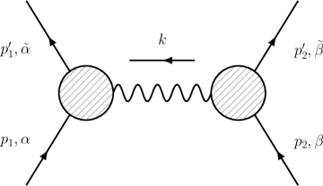
Figure 1: Residue of tree-level four-point scattering amplitude in $t$ channel

The classical limit is dominated by small momentum transfer

$$t=k^{2}=\hbar^{2}\bar{k}^{2}.$$ (69)

where the tree-level four-point amplitude is factorized into two three-point ones:

$${\cal A}^{(0)}(p_{1}^{\prime},\alpha;p_{2}^{\prime},\beta|p_{1},\alpha;p_{2},\beta)=-\frac{1}{\hbar^{2}\bar{k}^{2}}\!\sum_{\pm} {\cal A}^{(0)}(p_{1}^{\prime},\alpha|p_{1},\alpha;k,\pm)$$ (70)

$$\times {\cal A}^{(0)}(p_{2}^{\prime},\beta;k,\mp|p_{2},\beta)+{\cal O}(1/\hbar),$$

as illustrated in figure 1. For real external momenta on the mass shell, $k$ is always spacelike. However, we may extract the $t$-channel residue by first considering complex on-shell momenta consistent with $k^{2}=0$ and then analytically continuing the result to real spacelike $k$, along the lines of the Holomorphic Classical Limit of ref. Guevara:2017csg .

3.1 Three-point amplitudes

Let us now focus on the classical limit of the three-point amplitude shown in figure 2

$${\cal A}_{3}^{h} \equiv{\cal A}^{(0)}(p_{2},\beta|p_{1},\alpha;k,h)$$ (71)

$$=e^{-(\|\alpha\|^{2}+\|\beta\|^{2})/2}\sum_{s_{1},s_{2}}\frac{(\tilde{\beta}_{b})^{\odot 2s_{2}}(\alpha^{a})^{\odot 2s_{1}}}{\sqrt{(2s_{1})!(2s_{2})!}}\cdot{\cal A}^{(0)\{b\}}{}_{\{a\}}(p_{2},s_{2}|p_{1},s_{1};k,h),$$

which we have relabeled with respect to the amplitudes appearing in eq. (70), so as to unclutter the notation within this subsection. Although we have allowed the angular-momentum spinors to be different for the incoming and outgoing massive states, we will keep in mind that, in view of the classical impulse formulae, we are particularly interested in the case where $\alpha=\beta$. Note, however, that the state expansion above involves a double summation over amplitudes with all possible combinations of incoming and outgoing massive spins. In fact, one can think of coherent-state amplitudes as generating functions for various definite-spin amplitudes, for instance

$${\cal A}^{(0)\{b\}}{}_{\{a\}}(p_{2},s_{2}|p_{1},s_{1};k,h)=\frac{1}{\sqrt{(2s_{1})!(2s_{2})!}}\bigg{[}\frac{\partial~{}}{\partial\tilde{\beta}_{b}}\bigg{]}^{\odot 2s_{2}}\bigg{[}\frac{\partial~{}}{\partial\alpha^{a}}\bigg{]}^{\odot 2s_{1}}{\cal A}_{3}^{h}\,\bigg{|}_{\alpha=\beta=0}.$$ (72)

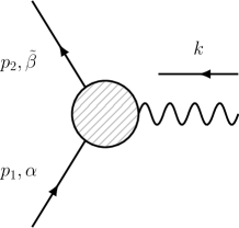
Figure 2: Tree-level three-point scattering amplitude

For concreteness, we work with the case of gravitational interaction. We start with the minimal-coupling amplitudes

$${\cal A}_{\text{min}}^{(0)\{b\}}{}_{\{a\}}(p_{2},s|p_{1},s;k,+) =-\frac{\kappa}{2}\frac{\langle 2^{b}1_{a}\rangle^{\odot 2s}\!}{m^{2s-2}}x^{2},$$ (73a)

$${\cal A}_{\text{min}}^{(0)\{b\}}{}_{\{a\}}(p_{2},s|p_{1},s;k,-) =(-1)^{2s+1}\frac{\kappa}{2}\frac{[2^{b}1_{a}]^{\odot 2s}\!}{m^{2s-2}}x^{-2},$$ (73b)

where $x$ is the unit-helicity factor that has multiple equivalent representations in terms of massless helicity spinors or polarization vectors:

$$x=\frac{[k|p_{1}|r\rangle}{m\langle k\;\!r\rangle}=\frac{m[k\;\!r]}{\langle k|p_{1}|r]}=-\frac{\sqrt{2}}{m}(p_{1}\cdot\varepsilon^{+})=\bigg{[}\frac{\sqrt{2}}{m}(p_{1}\cdot\varepsilon^{-})\bigg{]}^{-1}.$$ (74)

These simplest general-spin amplitudes were proposed by Arkani-Hamed, Huang and Huang Arkani-Hamed:2017jhn based on their tame behavior in the massless limit, but were soon realized Guevara:2018wpp ; Chung:2018kqs to correspond to scattering of Kerr’s rotating black hole (also obtained by means of on-shell heavy particle theories Aoude:2020onz ). Let us derive this result in our current formalism.

3.2 From minimal coupling to Kerr

The minimal-coupling amplitudes correspond to the diagonal slice $s_{1}=s_{2}=s$ of the summation in the total-spin quantum numbers, so their contribution to the coherent-spin amplitude (71) is simply

$${\cal A}_{3,\text{min}}^{+} =-\frac{\kappa}{2}x^{2}e^{-(\|\alpha\|^{2}+\|\beta\|^{2})/2}\sum_{2s=0}^{\infty}\frac{1}{(2s)!}(\tilde{\beta}_{b})^{\odot 2s}\cdot\frac{\langle 2^{b}1_{a}\rangle^{\odot 2s}\!}{m^{2s-2}}\cdot(\alpha^{a})^{\odot 2s}$$ (75)

$$=-\frac{\kappa}{2}m^{2}x^{2}e^{-(\|\alpha\|^{2}+\|\beta\|^{2})/2}\exp\bigg{\{}\frac{1}{m}\tilde{\beta}_{b}\langle 2^{b}1_{a}\rangle\alpha^{a}\bigg{\}}.$$

Recall that in section 2.3.4 we boosted the initial- and final-state spin operators to the same intermediate momentum $p_{\rm a}$. In the same spirit, we are now going to determine the dependence of the above exponent on the angular-momentum operator $S_{p_{\rm a}}^{\mu}$, which generates the little group of the average momentum $p_{\rm a}=(p_{1}+p_{2})/2=p_{1}+k/2$. The three-point on-shell kinematics implies that this momentum is also on-shell due to $p_{1}\cdot k=p_{2}\cdot k=p_{\rm a}\cdot k=0$, and it is related to $p_{1}$ and $p_{2}$ via boosts

$$p_{1}^{\rho}=\exp\!\bigg{[}{-}\frac{ip_{\rm a}^{\mu}k^{\nu}\!}{2m^{2}}\Sigma_{\mu\nu}\bigg{]}^{\rho}_{~{}\sigma}p_{\rm a}^{\sigma},\qquad\quad p_{2}^{\rho}=\exp\!\bigg{[}\frac{ip_{\rm a}^{\mu}k^{\nu}\!}{2m^{2}}\Sigma_{\mu\nu}\bigg{]}^{\rho}_{~{}\sigma}p_{\rm a}^{\sigma}.$$ (76)

The initial- and final-state spinors may be similarly boosted using the chiral Lorentz generators $\sigma^{\mu\nu}=i\sigma^{[\mu}\bar{\sigma}^{\nu]}/2$:

$$|1_{a}\rangle =U_{a}{}^{b}(p_{1},p_{\rm a})\exp\!\bigg{[}{-}\frac{ip_{\rm a}^{\mu}k^{\nu}\!}{2m^{2}}\sigma_{\mu\nu}\bigg{]}|{\rm a}_{b}\rangle=U_{a}{}^{b}(p_{1},p_{\rm a})\bigg{(}|{\rm a}_{b}\rangle-\frac{1}{4m}|k|{\rm a}_{b}]\bigg{)},$$ (77)

$$|2^{a}\rangle =U^{a}{}_{b}(p_{2},p_{\rm a})\exp\!\bigg{[}\frac{ip_{\rm a}^{\mu}k^{\nu}\!}{2m^{2}}\sigma_{\mu\nu}\bigg{]}|{\rm a}^{b}\rangle~{}~{}\Rightarrow~{}~{}\langle 2^{a}|=U^{a}{}_{b}(p_{2},p_{\rm a})\bigg{(}\langle{\rm a}^{b}|-\frac{1}{4m}[{\rm a}^{b}|k|\bigg{)},$$

where we have used the nilpotency of $p_{\rm a}^{\mu}k^{\nu}\sigma_{\mu\nu}$ for $k^{2}=0$. Recalling the mild momentum dependence (37) of the ${\rm SU}(2)$ spinors, as well as the properties of ${\rm SU}(2)$ transformations pointed out in footnote 4, we may rewrite the exponent in (75) as

$$\tilde{\beta}_{b}(p_{2})\langle 2^{b}1_{a}\rangle\alpha^{a}(p_{1}) =\tilde{\beta}_{b}(p_{\rm a})\bigg{(}\langle{\rm a}^{b}{\rm a}_{a}\rangle-\frac{1}{4m}\Big{(}[{\rm a}^{b}|k|{\rm a}_{a}\rangle+\langle{\rm a}^{b}|k|{\rm a}_{a}]\Big{)}\!\bigg{)}\alpha^{a}(p_{\rm a}).$$ (78)

Here $\langle{\rm a}^{b}{\rm a}_{a}\rangle=m\delta_{a}^{b}$, and we may recognize the ${\rm SU}(2)$ spin generator

$$\sigma_{p_{\rm a}}^{\mu,a}{}_{b}=\frac{1}{2m}\Big{(}\langle{\rm a}^{a}|\sigma^{\mu}|{\rm a}_{b}]+[{\rm a}^{a}|\bar{\sigma}^{\mu}|{\rm a}_{b}\rangle\Big{)},$$ (79)

showing the separation between spinless and spin effects.

Having thus evaluated the positive-helicity amplitude (75), for completeness we display the coherent-spin amplitudes for both graviton helicities:

$${\cal A}_{3,\text{min}}^{\pm}=-\frac{\kappa}{2}m^{2}x^{\pm 2}e^{-(\|\alpha\|^{2}+\|\beta\|^{2})/2+\tilde{\beta}\alpha}\exp\bigg{\{}{\mp}\frac{\hbar}{2m}\bar{k}_{\mu}(\tilde{\beta}\>\!\sigma_{p_{\rm a}}^{\mu}\;\!\!\alpha)\bigg{\}},$$ (80)

where all spinors are understood to correspond to the little group of $p_{\rm a}$. A remarkable property here is that we have factored out the standard coherent-state overlap function

$$\langle\beta|\alpha\rangle=e^{-(\|\alpha\|^{2}+\|\beta\|^{2})/2+\tilde{\beta}\alpha}.$$ (81)

Note that in the classical limit of the four-point amplitude (70) we take $\tilde{\beta}_{a}=(\alpha^{a})^{*}$ and can therefore identify the spin expectation value (34a):

$${\cal A}_{3,\text{min}}^{\pm}\big{|}_{\beta=\alpha}=-\frac{\kappa}{2}m^{2}x^{\pm 2}\exp\bigg{\{}{\mp}\frac{1}{m}\bar{k}_{\mu}\langle S_{p_{\rm a}}^{\mu}\rangle_{\alpha}\bigg{\}}=-\frac{\kappa}{2}m^{2}x^{\pm 2}e^{\mp\bar{k}\cdot a_{\rm a}}.$$ (82)

Importantly, this result would have been classically vanishing if the exponential suppression by the original prefactor $e^{-(\|\alpha\|^{2}+\|\beta\|^{2})/2}=e^{-\|\alpha\|^{2}}$, as $\|\alpha\|^{2}$ grows as $1/\hbar$, had not been canceled by the exponential growth of $e^{\tilde{\beta}\alpha}=e^{\|\alpha\|^{2}}$.

3.2.1 Connection to Kerr black hole

The exponential spin-multipole structure that we have obtained is a firm basis for the identification of the minimal-coupling amplitudes with gravitational scattering of black holes. The argument for this is given in refs. Guevara:2018wpp ; Guevara:2019fsj and is based on the classical stress-energy tensor Vines:2017hyw

$$T^{\mu\nu}_{\text{Kerr}}(x)=m\!\int\!d\tau\;\!u^{(\mu}\exp(a*\partial)^{\nu)}{}_{\rho}u^{\rho}\delta^{4}(x-u\tau),$$ (83)

which in linearized gravity serves as an effective source for a Kerr black hole with mass $m$, velocity $u^{\mu}$ and spin length $a^{\mu}$. The exponential $e^{a*\partial}$, involving the Levi-Civita contraction

$$(a*b)^{\mu\nu}=\epsilon^{\mu\nu\alpha\beta}a_{\alpha}b_{\beta},$$ (84)

may be shown to yield precisely $e^{\mp\bar{k}\cdot a_{\rm a}}$ when coupled to an on-shell graviton (see appendix A for a matching calculation encompassing the Kerr case). In fact, formulae identical to the right-hand side of eq. (82) appeared in ref. Guevara:2019fsj but featured chiral-spinor versions of the Pauli-Lubanski operator (26) instead of the spin expectation value $a_{\rm a}^{\mu}$. An obvious advantage of our current approach is that it enables us to directly identify the classical spin vector right away, instead of heuristically replacing quantum-mechanical operators with the corresponding classical quantities.

3.2.2 Multipoles from lower spins

As first noticed in ref. Vaidya:2014kza , lower spin-induced black-hole multipoles may be extracted from considering particles with finite quantum spin. Namely, the $2^{2s}$-pole interaction appears for spin-$s$ particles. To see how this occurs in our formalism, let us truncate the exponential (75) in the argument above:

$${\cal A}_{3,\text{min}}^{+,\text{trunc}}\big{|}_{\beta=\alpha}=-\frac{\kappa}{2}x^{2}e^{-\|\alpha\|^{2}}\sum_{2s=0}^{r}\frac{1}{(2s)!}(\tilde{\alpha}_{b}(p_{2}))^{\odot 2s}\cdot\frac{\langle 2^{b}1_{a}\rangle^{\odot 2s}\!}{m^{2s-2}}\cdot(\alpha^{a}(p_{1}))^{\odot 2s}$$

$$=-\frac{\kappa}{2}m^{2}x^{2}e^{-\|\alpha\|^{2}}\sum_{2s=0}^{r}\frac{1}{(2s)!}(\tilde{\alpha}_{b}(p_{\rm a}))^{\odot 2s}\!\cdot\bigg{(}\delta^{b}_{a}-\frac{\hbar}{2m}\bar{k}_{\mu}\sigma_{p_{\rm a}}^{\mu,b}{}_{a}\!\bigg{)}^{\!\odot 2s}\!\!\cdot(\alpha^{a}(p_{\rm a}))^{\odot 2s}$$ (85)

$$=-\frac{\kappa}{2}m^{2}x^{2}e^{-\|\alpha\|^{2}}\sum_{2s=0}^{r}\sum_{n=0}^{2s}\frac{(\tilde{\alpha}_{b}(p_{\rm a}))^{\odot 2s}\!}{n!(2s-n)!}\cdot\bigg{(}{-}\frac{\hbar}{2m}\bar{k}\cdot\sigma_{p_{\rm a}}^{~{}\,b}{}_{a}\!\bigg{)}^{\!\odot n}\!\!\odot(\delta^{b}_{a})^{\odot(2s-n)}\!\cdot(\alpha^{a}(p_{\rm a}))^{\odot 2s}.$$

To deal with this truncated sum, we may use the following property of the quantum angular-momentum representation (31), true for any lightlike $k$ satisfying $p\cdot k=0$:

$$\big{[}(k\cdot S_{p})^{n}\big{]}^{s,\{a\}}{}_{s^{\prime},\{b\}}=\frac{\hbar^{n}(2s)!}{2^{n}(2s-n)!}\;\!\delta^{s}_{s^{\prime}}\big{(}k\cdot\sigma_{p}{}^{a}{}_{b}\big{)}^{\odot n}\odot\big{(}\delta^{a}_{b}\big{)}^{\odot(2s-n)}.$$ (86)

Whenever $n>2s$, the gamma function $\Gamma(2s-n+1)=(2s-n)!$ in the denominator develops poles, implying that the right-hand side then vanishes, so we can still obtain an exponential:

$${\cal A}_{3,\text{min}}^{+,\text{trunc}}\big{|}_{\beta=\alpha} =-\frac{\kappa}{2}m^{2}x^{2}e^{-\|\alpha\|^{2}}\sum_{2s=0}^{r}\frac{1}{(2s)!}\sum_{n=0}^{2s}\frac{1}{n!}(\tilde{\alpha}_{b})^{\odot 2s}\!\cdot\!\bigg{[}\bigg{(}{-}\frac{1}{m}\bar{k}\cdot S_{p_{\rm a}}\bigg{)}^{\!n}\bigg{]}^{\{b\}}_{~{}\;\;\;\{a\}}\!\!\cdot(\alpha^{a})^{\odot 2s}$$

$$=-\frac{\kappa}{2}m^{2}x^{2}e^{-\|\alpha\|^{2}}\sum_{2s=0}^{r}\frac{1}{(2s)!}(\tilde{\alpha}_{b})^{\odot 2s}\!\cdot\exp\!\bigg{[}{-}\frac{1}{m}\bar{k}\cdot S_{p_{\rm a}}\bigg{]}^{\{b\}}_{~{}\;\;\;\{a\}}\!\!\cdot(\alpha^{a})^{\odot 2s}$$

$$=-\frac{\kappa}{2}m^{2}x^{2}e^{-\|\alpha\|^{2}}\sum_{2s=0}^{r}\frac{\|\alpha\|^{4s}}{(2s)!}\bigg{\langle}\!\exp\!\bigg{[}{-}\frac{1}{m}\bar{k}\cdot S_{p_{\rm a}}\bigg{]}\bigg{\rangle}_{\!2s},$$ (87)

where we have used a finite-spin expectation value defined in an obvious way as $\langle O\rangle_{2s}=(\tilde{\alpha}_{a})^{\odot 2s}\cdot O^{s,\{a\}}{}_{s^{\prime}=s,\{b\}}\cdot(\alpha^{b})^{\odot 2s}/\|\alpha\|^{4s}$. For any finite truncation $r$, taking $\|\alpha\|~{}\to~{}\infty$ according to the classical limit (47c) would nullify the coherent-spin amplitude. Moreover, for any finite $s=0,1/2,\dots,r/2$, the spin exponential in eq. (87) is naturally truncated at the $2^{2s}$ multipole, exactly as in refs. Guevara:2018wpp ; Guevara:2019fsj ; Aoude:2020onz . However, if we presume a classical-limit property of the type (34b), we may recognize that the multipoles which are present in the finite-spin contributions above very well correspond to those in our full result (82) — except for the summation over $s$ and the normalization prefactors $e^{-\|\alpha\|^{2}}\|\alpha\|^{4s}/(2s)!$, which are important in the coherent-spin formalism but should rather be ignored in a finite-spin approach.

3.3 Non-minimal coupling

Now that we have explored how the multipole structure of a Kerr black hole arises from the minimal-coupling amplitudes, we may as well consider more general massive particles which couple to gravity in a non-minimal way. We write the corresponding three-point amplitudes still for equal spins but otherwise in full generality as Arkani-Hamed:2017jhn

$${\cal A}_{\text{gen}}^{(0)\{b\}}{}_{\{a\}}(p_{2},s|p_{1},s;k,+) =-\frac{\kappa}{2}\sum_{n=0}^{2s}g_{n}^{+}\frac{x^{n+2}\langle 2^{b}1_{a}\rangle^{\odot(2s-n)}\!}{m^{2s+n-2}}\odot\big{(}\langle 2^{b}k\rangle\langle k\>\!1_{a}\rangle\big{)}^{\odot n},$$ (88)

$${\cal A}_{\text{gen}}^{(0)\{b\}}{}_{\{a\}}(p_{2},s|p_{1},s;k,-) =(-1)^{2s+1}\frac{\kappa}{2}\sum_{n=0}^{2s}g_{n}^{-}\frac{x^{-n-2}[2^{b}1_{a}]^{\odot(2s-n)}\!}{m^{2s+n-2}}\odot\big{(}[2^{b}k][k\>\!1_{a}]\big{)}^{\odot n}.$$

The dimensionless coupling constants $g_{n}^{+}$ and $g_{n}^{-}$ are understood to be related by complex conjugation due to parity conservation. Moreover, as we have seen above and will be able to further confirm below, the minimal couplings $g_{0}^{\pm}$ determine the gravitational interaction at zero spin and are therefore pegged to unity by the equivalence principle. Importantly, we assume that the coupling constants $g_{n>0}^{\pm}$ depend only on their “non-minimalness” $n$ and not on the spin quantum number $s$.

Let us construct the non-minimal coherent-spin amplitude for positive helicity:

$${\cal A}_{3,\text{gen}}^{+} =-\frac{\kappa}{2}e^{-(\|\alpha\|^{2}+\|\beta\|^{2})/2}\sum_{2s=0}^{\infty}\sum_{n=0}^{2s}\frac{g_{n}^{+}x^{n+2}}{(2s)!m^{2s+n-2}}\big{(}\tilde{\beta}_{b}\langle 2^{b}1_{a}\rangle\alpha^{a}\big{)}^{2s-n}\big{(}\tilde{\beta}_{b}\langle 2^{b}k\rangle\langle k\>\!1_{a}\rangle\alpha^{a}\big{)}^{n}$$

$$=-\frac{\kappa}{2}m^{2}x^{2}e^{-(\|\alpha\|^{2}+\|\beta\|^{2})/2}\sum_{n=0}^{\infty}g_{n}^{+}x^{n}\bigg{(}\frac{\tilde{\beta}_{b}\langle 2^{b}k\rangle\langle k\>\!1_{a}\rangle\alpha^{a}}{m\>\!\tilde{\beta}_{b}\langle 2^{b}1_{a}\rangle\alpha^{a}}\bigg{)}^{\!n}\sum_{2s=n}^{\infty}\frac{\big{(}\tilde{\beta}_{b}\langle 2^{b}1_{a}\rangle\alpha^{a}\big{)}^{2s}\!}{(2s)!m^{2s}}$$

$$=-\frac{\kappa}{2}m^{2}x^{2}e^{-(\|\alpha\|^{2}+\|\beta\|^{2})/2}\exp\bigg{\{}\frac{1}{m}\tilde{\beta}_{b}\langle 2^{b}1_{a}\rangle\alpha^{a}\bigg{\}}$$ (89)

$$\qquad\>\!\!\times\sum_{n=0}^{\infty}g_{n}^{+}x^{n}\bigg{(}\frac{\tilde{\beta}_{b}\langle 2^{b}k\rangle\langle k\>\!1_{a}\rangle\alpha^{a}}{m\>\!\tilde{\beta}_{b}\langle 2^{b}1_{a}\rangle\alpha^{a}}\bigg{)}^{\!n}\bigg{[}1-\frac{1}{(n-1)!}\Gamma\bigg{(}n,\frac{1}{m}\tilde{\beta}_{b}\langle 2^{b}1_{a}\rangle\alpha^{a}\bigg{)}\bigg{]},$$

where changing the order of summation allowed us to evaluate the sum in the total-spin quantum number $s$. Setting $\tilde{\beta}_{a}=(\alpha^{a})^{*}$, we can again identify

$$\frac{1}{m}\tilde{\alpha}_{b}(p_{2})\langle 2^{b}1_{a}\rangle\alpha^{a}(p_{1})=\|\alpha\|^{2}-\bar{k}\cdot a_{\rm a},$$ (90)

as in section 3.2. In addition, we will now also need the equalities

$$x\;\!\tilde{\alpha}_{b}(p_{2})\langle 2^{b}k\rangle\langle k\>\!1_{a}\rangle\alpha^{a}(p_{1})=x^{-1}\tilde{\alpha}_{b}(p_{2})[2^{b}k][k\>\!1_{a}]\alpha^{a}(p_{1})=2m^{2}(\bar{k}\cdot a_{\rm a}).$$ (91)

They may be proven by using the three-point spinorial identities

$$[2^{b}1_{a}]=-\langle 2^{b}1_{a}\rangle-\frac{x}{m}\langle 2^{b}k\rangle\langle k\>\!1_{a}\rangle,\qquad\quad[2^{b}k]=x\langle 2^{b}k\rangle,\qquad\quad[k\>\!1_{a}]=x\langle k\>\!1_{a}\rangle,$$ (92)

together with the parity-conjugated version of eq. (90)

$$-\frac{1}{m}\tilde{\alpha}_{b}(p_{2})[2^{b}1_{a}]\alpha^{a}(p_{1})=\|\alpha\|^{2}+\bar{k}\cdot a_{\rm a},$$ (93)

which was implicitly used earlier to arrive at the negative-helicity version of eq. (80). In this way, we obtain

$$\!\!{\cal A}_{3,\text{gen}}^{\pm}\big{|}_{\beta=\alpha}\!=-\frac{\kappa}{2}m^{2}x^{\pm 2}e^{\mp\bar{k}\cdot a_{\rm a}}\!\sum_{n=0}^{\infty}g_{n}^{\pm}\bigg{[}\frac{\pm 2\bar{k}\cdot a_{\rm a}}{\|\alpha\|^{2}\mp\bar{k}\cdot a_{\rm a}}\bigg{]}^{\!n}\Bigg{[}1-\frac{\Gamma\big{(}n,\|\alpha\|^{2}\mp\bar{k}\cdot a_{\rm a}\big{)}}{(n-1)!}\Bigg{]},\!$$ (94)

where we have again displayed both helicity amplitudes for completeness. In the classical limit (47c), the gamma-function term is exponentially suppressed, since $\Gamma(n,\|\alpha\|^{2})\sim\|\alpha\|^{2(n-1)}e^{-\|\alpha\|^{2}}$ as $\|\alpha\|\to\infty$. Even still, the non-minimal couplings $g_{n>0}^{\pm}$ seem to be polynomially suppressed by $\|\alpha\|^{-2n}$.

This means that, in order to be able to model a classically spinning massive object with generic spin-induced multipoles using a quantum particle, one needs to introduce non-minimal coupling constants $g_{n>0}^{\pm}$ that scale as ${\cal O}(\hbar^{-n})$. In general relativity, the dynamics of such classical objects is conveniently described by the worldline effective theory, in which the spin-induced multipole contributions linear in the curvature tensor enter via the interaction Lagrangian Porto:2006bt ; Porto:2008tb ; Levi:2015msa

$$S_{R}=m\!\int\!d\tau\bigg{[} \sum_{n=1}^{\infty}\frac{(-1)^{n}}{(2n)!}C_{{\rm ES}^{2n}}(a\cdot\nabla)^{2n-2}R_{\lambda\mu\,\nu\rho}u^{\lambda}a^{\mu}u^{\nu}a^{\rho}$$ (95)

$$+\sum_{n=1}^{\infty}\frac{(-1)^{n}}{(2n+1)!}C_{{\rm BS}^{2n+1}}(a\cdot\nabla)^{2n-1}\,{}^{*}\!R_{\lambda\mu\,\nu\rho}u^{\lambda}a^{\mu}u^{\nu}a^{\rho}\bigg{]}_{x=r(\tau)},$$

where ${}^{*}\!R_{\lambda\mu\,\nu\rho}=\sqrt{-g}\;\!\epsilon_{\lambda\mu\sigma\tau}R^{\sigma\tau}{}_{\nu\rho}/2$, and $r^{\mu}(\tau)$, $u^{\mu}(\tau)=dr^{\mu}/d\tau$ and $a^{\mu}(\tau)$ are the coordinate, velocity and spin functions of proper time, respectively. In fact, it is possible to establish a correspondence between our non-minimal couplings $g_{n>0}^{\pm}$ and the dimensionless worldline Wilson coefficients $C_{{\rm ES}^{2n}}$ and $C_{{\rm BS}^{2n+1}}$. To do this, here we rely on the scattering amplitude

$${\cal A}^{\pm}_{\text{gen}}(p,k)=-\frac{\kappa}{2}m^{2}x^{\pm 2}\bigg{[}\sum_{n=0}^{\infty}\frac{C_{{\rm ES}^{2n}}}{(2n)!}(\bar{k}\cdot a)^{2n}\pm\sum_{n=0}^{\infty}\frac{C_{{\rm BS}^{2n+1}}}{(2n+1)!}(\bar{k}\cdot a)^{2n+1}\bigg{]},$$ (96)

which follows from the worldline action above and is derived in appendix A. The classical limit of the amplitude (94) may be reorganized in a similar fashion:

$${\cal A}_{3,\text{gen}}^{\pm}\big{|}_{\beta=\alpha} =-\frac{\kappa}{2}m^{2}x^{\pm 2}e^{\mp\bar{k}\cdot a_{\rm a}}\!\sum_{n=0}^{\infty}g_{n}^{\pm}\bigg{[}\frac{\pm 2\bar{k}\cdot a_{\rm a}}{\|\alpha\|^{2}}\bigg{]}^{\!n}$$ (97)

$$=-\frac{\kappa}{2}m^{2}x^{\pm 2}\sum_{n=0}^{\infty}\big{(}{\mp}\bar{k}\cdot a_{\rm a}\big{)}^{n}\sum_{r=0}^{n}\frac{(-2)^{r}g_{r}^{\pm}}{(n-r)!\|\alpha\|^{2r}}.$$

We can therefore read off the worldline Wilson coefficients implied by the non-minimal amplitudes (88):

$$C_{{\rm ES}^{2n}}=\sum_{r=0}^{2n}\frac{(2n)!(-2)^{r}g_{r}^{\pm}}{(2n-r)!\|\alpha\|^{2r}},\qquad\quad C_{{\rm BS}^{2n+1}}=-\sum_{r=0}^{2n+1}\frac{(2n+1)!(-2)^{r}g_{r}^{\pm}}{(2n-r+1)!\|\alpha\|^{2r}}.$$ (98)

This matching clearly requires that $g_{n}^{+}$ and $g_{n}^{-}$ be real and equal to each other. Moreover, let us point out the fact that, as explained in appendix A, in passing from the action (95) to the amplitude (96) we had to introduce the $n=0$ terms with $C_{{\rm ES}^{0}}=-C_{{\rm BS}^{1}}=1$, which unequivocally follow from the worldline kinetic terms. Hence

$$g_{0}^{\pm}=C_{{\rm ES}^{0}}=1,\qquad\quad g_{1}^{\pm}=\|\alpha\|^{2}(C_{{\rm BS}^{1}}+g_{0}^{\pm})/2=0.$$ (99)

The crucial feature of the Wilson-coefficient map (98) is that, in order to describe a generic classical particle using the three-point amplitudes (88), one must consider the non-minimal coupling constants $g_{n>0}$ that depend on the classical spin length $a$ of the particle via

$$\|\alpha\|^{2}=\frac{2m}{\hbar}\sqrt{-a^{2}}.$$ (100)

The only gravitational objects escaping this rule seem to be black holes, for which $g_{0}^{\pm}=1$ and $g_{n>0}^{\pm}=0$.

In this section, we have naturally landed on equal coefficients $g_{n}^{+}=g_{n}^{-}$ for positive- and negative- helicity amplitudes. Non-equal coefficients can be motivated by the electric-magnetic duality, which in electromagnetism mixes the electric and magnetic charges. The gravitational electric-magnetic duality relates the mass and NUT charge parameter in a similar manner Henneaux:2004jw . Together with double copy and the Newman-Janis shift Newman:1965tw , the duality generates a whole web of theories described in refs. Huang:2019cja ; Emond:2020lwi , in which the three-point coupling coefficients $g_{n}^{\pm}$ develop complex phases while still being related by complex conjugation.

3.4 Unequal spin amplitudes

So far we have been focusing on the diagonal slice $s_{1}=s_{2}$ of the double sum in the three-point coherent-spin amplitude (71). This is because, as we will show in this section, the off-diagonal contributions vanish in the classical limit, or at least may be considered to vanish unless certain artificial assumptions are made beforehand.

For concreteness, let us consider the positive-helicity amplitudes with $s_{1}>s_{2}$, which may be written in full generality as Arkani-Hamed:2017jhn

$${\cal A}_{s_{1}>s_{2}}^{(0)\{b\}}{}_{\{a\}}(p_{2},s_{2}|p_{1},s_{1};k,+) =-\frac{\kappa}{2}\sum_{n=0}^{2s_{2}}g_{n,s_{1},s_{2}}\frac{x^{s_{1}-s_{2}+n+2}}{m^{2s_{1}+n-2}}$$ (101)

$$\qquad\!\times\langle 2^{b}1_{a}\rangle^{\odot(2s_{2}-n)}\odot\langle 2^{b}k\rangle^{\odot n}\odot\langle k\>\!1_{a}\rangle^{\odot(2s_{1}-2s_{2}+n)}.$$

Dressing it with coherent states gives

$${\cal A}_{3,s_{1}>s_{2}}^{+} =-\frac{\kappa}{2}m^{2}x^{2}e^{-(\|\alpha\|^{2}+\|\beta\|^{2})/2}\!\sum_{2s_{2}=0}^{\infty}\,\sum_{2s_{1}=2s_{2}+1}^{\infty}\,\sum_{n=0}^{2s_{2}}\frac{g_{n,s_{1},s_{2}}x^{s_{1}-s_{2}+n}}{\sqrt{(2s_{1})!(2s_{2})!}m^{2s_{1}+n}}$$ (102)

$$\qquad\,\qquad\times\big{(}\tilde{\beta}_{b}\langle 2^{b}1_{a}\rangle\alpha^{a}\big{)}^{2s_{2}-n}\big{(}\tilde{\beta}_{b}\langle 2^{b}k\rangle\langle k\>\!1_{a}\rangle\alpha^{a}\big{)}^{n}\big{(}\langle k\>\!1_{a}\rangle\alpha^{a}\big{)}^{2(s_{1}-s_{2})}.$$

We are now interested in the behavior of the above triple sum in the classical limit, in which

$$\|\alpha\|={\cal O}(\hbar^{-1/2})=\|\beta\|,\qquad\quad|k\rangle={\cal O}(\hbar^{1/2}).$$ (103)

So the only factor that has a chance to counteract the vanishing of the exponential prefactor is the term

$$\frac{1}{m}\tilde{\beta}_{b}(p_{2})\langle 2^{b}1_{a}\rangle\alpha^{a}(p_{1})=\tilde{\beta}_{a}(p_{\rm a})\alpha^{a}(p_{\rm a})-\frac{1}{m}\bar{k}_{\mu}\langle\beta|S_{p_{\rm a}}^{\mu}|\alpha\rangle,$$ (104)

in which the second contribution is classically finite but the first one grows as ${\cal O}(1/\hbar)$. Indeed, we have seen in section 3.2 how this contribution can in principle combine with the exponential prefactor to produce the coherent-state overlap $\langle\beta|\alpha\rangle$, which is finite unless $\|\alpha-\beta\|\to\infty$, as follows from $|\langle\beta|\alpha\rangle|^{2}=e^{-\|\alpha-\beta\|^{2}}$. Let us therefore denote the finite dimensionless contributions ${\cal O}(\hbar^{0})$ as

$$\frac{\tilde{\beta}_{b}(p_{2})\langle 2^{b}1_{a}\rangle\alpha^{a}(p_{1})}{m\tilde{\beta}_{a}(p_{\rm a})\alpha^{a}(p_{\rm a})}=A,\quad\frac{x}{m^{2}}\tilde{\beta}_{b}(p_{2})\langle 2^{b}k\rangle\langle k\>\!1_{a}\rangle\alpha^{a}(p_{1})=B,\quad\frac{\sqrt{x}}{m}\langle k\>\!1_{a}\rangle\alpha^{a}(p_{1})=C,$$ (105)

in terms of which the amplitude contribution writes

$$\!\!{\cal A}_{3,s_{1}>s_{2}}^{+}\!=-\frac{\kappa}{2}m^{2}x^{2}e^{-(\|\alpha\|^{2}+\|\beta\|^{2})/2}\!\sum_{2s_{2}=0}^{\infty}\sum_{r=1}^{\infty}\sum_{n=0}^{2s_{2}}\frac{g_{n,s_{2}+r/2,s_{2}}B^{n}C^{r}}{\sqrt{(2s_{2}+r)!(2s_{2})!}}\big{(}A\tilde{\beta}_{a}\alpha^{a}\big{)}^{2s_{2}-n}\!.\!$$ (106)

Moreover, although we have allowed the coupling constants $g_{n,s_{1},s_{2}}$ to depend on the spin quantum numbers, in the following estimations let us replace them with

$$y_{n}\equiv\sup_{s_{1}>s_{2}}|g_{n,s_{1},s_{2}}|.$$ (107)

This is going to allow us to change the order of summation:

$$\bigg{|}\frac{2{\cal A}_{3,s_{1}>s_{2}}^{+}}{\kappa\;\!m^{2}x^{2}}\bigg{|} \leq e^{-(\|\alpha\|^{2}+\|\beta\|^{2})/2}\sum_{n=0}^{\infty}\frac{y_{n}|B|^{n}}{|A\tilde{\beta}_{a}\alpha^{a}|^{n}}\sum_{r=1}^{\infty}|C|^{r}\!\sum_{2s_{2}=n}^{\infty}\!\frac{|A\tilde{\beta}_{a}\alpha^{a}|^{2s_{2}}}{\sqrt{(2s_{2}+r)!(2s_{2})!}}.$$ (108)

In order to deal with the square roots of the factorials, we use the following inequality

$$(t+r)!\,t!=\Gamma(t+r+1)\,\Gamma(t+1)~{}>~{}\Gamma^{2}(t+3/2)\,\Gamma(r),\qquad\quad t,r=1,2,\ldots$$ (109)

The resulting sum may be evaluated using

$$\sum_{t=n}^{\infty}\frac{a^{t}}{\Gamma(t+3/2)}=\frac{e^{a}}{\sqrt{a}}\bigg{[}1-\frac{\Gamma(n+1/2,a)}{\Gamma(n+1/2)}\bigg{]}<\frac{e^{a}}{\sqrt{a}},\qquad\quad a>0.$$ (110)

Hence our estimation becomes

$$\bigg{|}\frac{2{\cal A}_{3,s_{1}>s_{2}}^{+}}{\kappa\;\!m^{2}x^{2}}\bigg{|}<e^{-(\|\alpha\|^{2}+\|\beta\|^{2})/2}\sum_{n=0}^{\infty}\frac{y_{n}|B|^{n}}{|A\tilde{\beta}_{a}\alpha^{a}|^{n}}\sum_{r=1}^{\infty}\frac{|C|^{r}}{\sqrt{(r-1)!}}\frac{\exp|A\tilde{\beta}_{a}\alpha^{a}|}{\sqrt{|A\tilde{\beta}_{a}\alpha^{a}|}}.$$ (111)

Here we may recall that $A\tilde{\beta}_{a}\alpha^{a}$ is precisely given by eq. (104), so we finally obtain

$$\big{|}{\cal A}_{3,s_{1}>s_{2}}^{+}\big{|}<\frac{\kappa}{2}m^{2}x^{2}\frac{e^{-(\|\alpha\|-\|\beta\|)^{2}/2}\!}{|\tilde{\beta}_{a}\alpha^{a}|^{1/2}}\exp\Big{|}\frac{1}{m}\bar{k}_{\mu}\langle\beta|S_{p_{\rm a}}^{\mu}|\alpha\rangle\Big{|}$$ (112)

$$\times\sum_{n=0}^{\infty}\frac{y_{n}|B|^{n}}{|\tilde{\beta}_{a}\alpha^{a}|^{n}\,|A|^{n+1/2}}\sum_{r=1}^{\infty}\frac{|C|^{r}}{\sqrt{(r-1)!}}$$ .

In the classical limit, we are interested in $\beta\approx\alpha$, including the case where $\tilde{\beta}_{a}=(\alpha^{a})^{*}$, which means that the relative “cosine” inside the inner product $\tilde{\beta}_{a}\alpha^{a}$ should be regarded as at least finite. Therefore, the product $\tilde{\beta}_{a}\alpha^{a}$ grows as ${\cal O}(1/\hbar)$. Similarly to situation with the equal-spin non-minimal couplings in section 3.3, the coupling-constants $y_{n}$ are accompanied by factors of $1/(\tilde{\beta}_{a}\alpha^{a})^{n}$ and are thus power-suppressed — unless they or their counterparts $g_{n,s_{1},s_{2}}$ are rescaled at the level of the scattering amplitude (101). For equal spins, however, such a rescaling procedure was motivated by the knowledge of classical multipole interactions, which could be modeled by proportionally amplified coupling constants. In addition, the crucial difference between equal and unequal spins is the presence of an overall factor $1/|\tilde{\beta}_{a}\alpha^{a}|^{1/2}={\cal O}(\hbar^{1/2})$ in the estimation (112), which means that even the “almost minimal” couplings $g_{0,s_{1},s_{2}}$ would need to scale as ${\cal O}(\hbar^{-1/2})$. Since we are not aware of classical interactions that would benefit from such an elaborate rescaling procedure — which in this case could not be consistently implemented by a $|k\rangle\to|\bar{k}\rangle$ switch, and moreover the classical interpretation of the expression $C=\sqrt{x}\langle k\>\!1_{a}\rangle\alpha^{a}/m$ seems rather obscure, we see no interest in trying to retain the non-equal spin couplings in the classical limit. We are thus vindicated for ignoring the off-diagonal contributions in the coherent-spin amplitude (71).

4 Elastic gravitational scattering

In this section we return to the four-point amplitude ${\cal A}^{(0)}(p_{1}^{\prime},\alpha;p_{2}^{\prime},\beta|p_{1},\alpha;p_{2},\beta)$, which determines the leading-order impulse and spin-kick observables via the formulae (56) and (67). We have already explained that the classical limit of this amplitude is naturally factorized into a product of two three-point amplitudes, as depicted in figure 1. Now that we have extensively dissected these lower-point ingredients, we may proceed to constructing the four-point amplitude.

For the sake of generality, we will use the “classical” amplitudes (96), which in appendix A are derived from the worldline effective action with free Wilson coefficients

$$C_{2n}\equiv C_{{\rm ES}^{2n}},\qquad\quad C_{2n+1}\equiv C_{{\rm BS}^{2n+1}}.$$ (113)

In view of the matching (98), we may easily reinterpret these amplitudes as the classical limit of the coherent-state amplitudes (94). After the above Wilson-coefficient relabeling, we can write them simply as

$${\cal A}^{(0)}(p_{1}^{\prime},\alpha|p_{1},\alpha;k,\pm)=-\frac{\kappa}{2}m_{\rm a}^{2}x_{\rm a}^{\pm 2}\sum_{n=0}^{\infty}\frac{C_{{\rm a}\>\!n}}{n!}\big{(}{\pm}\bar{k}\cdot a_{\rm a}\big{)}^{n}+{\cal O}(\hbar^{0}),$$ (114)

and similarly for particle ${\rm b}$, except a sign switch for $\bar{k}$. If we plug these amplitudes into eq. (70), we run into the helicity-factor ratios, which on the $t$-channel pole kinematics evaluate to

$$x_{\rm a}/x_{\rm b}=\gamma(1-v),\qquad\quad x_{\rm b}/x_{\rm a}=\gamma(1+v).$$ (115)

Here we have used the relative Lorentz factor $\gamma$ and the corresponding velocity $v$ defined by

$$\gamma=\frac{1}{\sqrt{1-v^{2}}}=\frac{p_{\rm a}\!\cdot p_{\rm b}}{m_{\rm a}m_{\rm b}}.$$ (116)

The physical meaning of these quantities is that in the rest frame of one of the incoming particles the other one moves with speed $v$, as in

$$\left\{\begin{aligned} p_{\rm a}^{\mu}&=\gamma m_{\rm a}(1,0,0,v),\\ p_{\rm b}^{\mu}&=(m_{\rm b},0,0,0),\end{aligned}\right.\qquad\overset{\begin{subarray}{c}\text{Lorentz boost}\\ ~{}\end{subarray}}{\Leftrightarrow}\qquad\left\{\begin{aligned} p_{\rm a}^{\mu}&=(m_{\rm a},0,0,0),\\ p_{\rm b}^{\mu}&=\gamma m_{\rm b}(1,0,0,-v).\end{aligned}\right.$$ (117)

Therefore, the classical limit of the elastic scattering amplitude (70) becomes

$${\cal A}^{(0)}(p_{1}^{\prime},\alpha;p_{2}^{\prime},\beta|p_{1},\alpha;p_{2},\beta)=-\frac{\kappa^{2}m_{\rm a}^{2}m_{\rm b}^{2}}{4\hbar^{2}\bar{k}^{2}}\sum_{\pm} \>\!\!\gamma^{2}(1\mp v)^{2}$$ (118)

$$\times\sum_{n_{1}=0}^{\infty}\frac{C_{{\rm a}\>\!n_{1}}}{n_{1}!}\big{(}{\pm}\bar{k}\cdot a_{\rm a}\big{)}^{n_{1}}\sum_{n_{2}=0}^{\infty} \frac{C_{{\rm b}\>\!n_{2}}}{n_{2}!}\big{(}{\pm}\bar{k}\cdot a_{\rm b}\big{)}^{n_{2}}+{\cal O}(\hbar^{-5/2}).$$

We are still not entirely ready to analytically continue this expression away from the $t$-channel pole kinematics, since it contains parity-odd products of the type $\bar{k}\cdot a$ — which make sense on the three-point kinematics and are naturally accompanied by the helicity-dependent signs, but are alien to real-valued classical physics. Note, for example, that in order to make the transition between a clearly parity-even action (95) and the amplitude expression (96) we need the three-point identity (170) involving the massless polarization vector. Now that we wish to go away from the on-shell kinematics for the graviton, using eq. (170) is not an option. There are, however, four-point identities which involve the Levi-Civita tensor and are valid on the $t$-channel pole kinematics, namely Guevara:2019fsj

$$i\epsilon_{\mu\nu\rho\sigma}p_{\rm a}^{\mu}p_{\rm b}^{\nu}\bar{k}^{\rho}a_{\rm a}^{\sigma}=m_{\rm a}m_{\rm b}\gamma v(\bar{k}\cdot a_{\rm a}),\qquad\quad i\epsilon_{\mu\nu\rho\sigma}p_{\rm a}^{\mu}p_{\rm b}^{\nu}\bar{k}^{\rho}a_{\rm b}^{\sigma}=m_{\rm a}m_{\rm b}\gamma v(\bar{k}\cdot a_{\rm b}).$$ (119)

For brevity, we follow ref. Vines:2017hyw in introducing the notation

$$w^{\mu\nu}=\frac{2p_{\rm a}^{[\mu}p_{\rm b}^{\nu]}}{m_{\rm a}m_{\rm b}\gamma v},\qquad\quad[w*a]_{\lambda}=(*w)_{\lambda\mu}a^{\mu}=\frac{\epsilon_{\lambda\mu\nu\rho}p_{\rm a}^{\mu}p_{\rm b}^{\nu}a^{\rho}}{m_{\rm a}m_{\rm b}\gamma v},$$ (120)

which allows us to write a new expression for the elastic scattering amplitude that may be understood beyond the $t$-channel pole kinematics:

$${\cal A}^{(0)}(p_{\rm a}\!+\!k/2,\alpha;p_{\rm b}\!-\!k/2,\beta|p_{\rm a}\!-\!k/2,\alpha;p_{\rm b}\!+\!k/2,\beta)=-\frac{8\pi Gm_{\rm a}^{2}m_{\rm b}^{2}\gamma^{2}}{\hbar^{3}\bar{k}^{2}}~{}~{}\>$$ (121)

$$\times\sum_{\pm}(1\mp v)^{2}\!\!\sum_{n_{1},n_{2}=0}^{\infty}\!\!\frac{C_{{\rm a}\>\!n_{1}}C_{{\rm b}\>\!n_{2}}\!}{n_{1}!n_{2}!}\big{(}{\pm}i\bar{k}\cdot[w*a_{\rm a}]\big{)}^{n_{1}}\big{(}{\pm}i\bar{k}\cdot[w*a_{\rm b}]\big{)}^{n_{2}} +{\cal O}(\hbar^{-5/2}).$$

4.1 Eikonal phase

Our formulae (56) and (67) for both of the leading-order impulse observables involve the eikonal Fourier transform of the above amplitude

$${\cal A}_{4}^{(0)}(b)=\int_{k}e^{-i\bar{k}\cdot b}{\cal A}^{(0)}(p_{\rm a}\!+\!k/2,\alpha;p_{\rm b}\!-\!k/2,\beta|p_{\rm a}\!-\!k/2,\alpha;p_{\rm b}\!+\!k/2,\beta),$$ (122)

where $\int_{k}$ is the measure (55). This object is widely referred to as the eikonal phase Bjerrum-Bohr:2018xdl ; Bern:2019nnu ; Bern:2019crd ; Bern:2020buy ; Aoude:2020ygw ; Kosmopoulos:2021zoq ; Bern:2021dqo ; Bjerrum-Bohr:2021vuf ; Bjerrum-Bohr:2021din . In view of the form of the integrand (121), let us proceed to computing the integrals

$$I^{(n)}_{\mu_{1}\dots\mu_{n}}(b_{\perp})=\int_{k}\frac{e^{-i\bar{k}\cdot b}}{\bar{k}^{2}}\bar{k}_{\mu_{1}}\!\cdots\bar{k}_{\mu_{n}}=\frac{\hbar^{2}}{4}\!\int\!\frac{d^{4}\bar{k}}{(2\pi)^{2}}\delta(p_{\rm a}\!\cdot\bar{k})\delta(p_{\rm b}\!\cdot\bar{k})\frac{e^{-i\bar{k}\cdot b_{\perp}}}{\bar{k}^{2}}\bar{k}_{\mu_{1}}\!\cdots\bar{k}_{\mu_{n}},$$ (123)

where we have extracted the Planck constants inherent to the eikonal measure. We have also taken care to indicate that these integrals only depend on $b_{\perp}^{\mu}=\Pi^{\mu}{}_{\nu}(p_{\rm a},p_{\rm b})b^{\nu}$, which lies in ${\rm E}^{\perp}_{p_{\rm a},p_{\rm b}}$, as opposed to the original impact parameter $b\in{\rm E}^{\perp}_{u_{\rm a},u_{\rm b}}$.

The simplest of these integrals is a scalar that may be computed in the center-of-mass (COM) frame, in which $\bar{k}$ is constrained to be $(0,\bar{k}^{1},\bar{k}^{2},0)\in{\rm E}^{\perp}_{p_{\rm a},p_{\rm b}}$. The result is

$$I^{(0)}(b_{\perp})=\frac{\hbar^{2}}{8\pi m_{\rm a}m_{\rm b}\gamma v}\Big{(}\log\sqrt{-b_{\perp}^{2}}+C_{\epsilon}\Big{)},\qquad\quad C_{\epsilon}=\log\frac{\epsilon}{2}+\gamma_{\text{Euler}}+{\cal O}(\epsilon^{2}).$$ (124)

where $C_{\epsilon}$ is a logarithmically divergent constant, which we wrote in terms of the infrared regulator $\epsilon<|\bar{\boldsymbol{k}}_{\perp}|$. Being interested in the observables, the formulae for which only depend on the derivatives of ${\cal A}^{(0)}(b)$, we may safely omit this infinite constant later. All of the tensor integrals (123) may now be obtained as partial derivatives

$$I_{(n)}^{\mu_{1}\dots\mu_{n}}(b_{\perp})=i^{n}\Pi^{\mu_{1}\nu_{1}}\cdots\Pi^{\mu_{n}\nu_{n}}\frac{\partial~{}}{\partial b_{\perp}^{\nu_{1}}}\cdots\frac{\partial~{}}{\partial b_{\perp}^{\nu_{n}}}I^{(0)}(b_{\perp}).$$ (125)

The projectors (58) are important to ensure that that the resulting expression stays transverse in all of its indices. In this way, one can obtain explicit answers like

$$I_{(1)}^{\mu}(b_{\perp})=\frac{i\hbar^{2}}{8\pi m_{\rm a}m_{\rm b}\gamma v}\frac{b_{\perp}^{\mu}}{b_{\perp}^{2}},\qquad\quad I_{(2)}^{\mu\nu}(b_{\perp})=\frac{-\hbar^{2}}{8\pi m_{\rm a}m_{\rm b}\gamma v}\frac{b_{\perp}^{2}\Pi^{\mu\nu}-2b_{\perp}^{\mu}b_{\perp}^{\nu}}{b_{\perp}^{4}},$$ (126)

which match those in e.g. ref. Maybee:2019jus . However, we choose to exploit the fact that the numerator of our amplitude (121) depends on $\bar{k}$ exclusively via $\bar{k}\cdot[w*a_{\rm a}]$, which already does the job of projecting the non-transverse components of any such integral for us. We may therefore write the eikonal phase (122) directly in terms of derivatives:

$${\cal A}_{4}^{(0)}(b)= -\frac{Gm_{\rm a}m_{\rm b}\gamma}{\hbar\>\!v}\sum_{\pm}(1\pm v)^{2}\!\!\sum_{n_{1},n_{2}=0}^{\infty}\!\!\frac{(\pm 1)^{n_{1}+n_{2}}\!}{n_{1}!n_{2}!}C_{{\rm a}\>\!n_{1}}C_{{\rm b}\>\!n_{2}}$$ (127)

$$~{}~{}\;\times\big{(}[w*a_{\rm a}]\cdot\partial_{b_{\perp}}\big{)}^{n_{1}}\big{(}[w*a_{\rm b}]\cdot\partial_{b_{\perp}}\big{)}^{n_{2}}\log\sqrt{-b_{\perp}^{2}}+{\cal O}(\hbar^{-1/2}).$$

As a cross-check, we can switch to Kerr scattering by setting $C_{{\rm a}\>\!n}=C_{{\rm b}\>\!n}=(-1)^{n}$. Then the infinite sums organize themselves into translation operators, and eq. (127) becomes

$${\cal A}_{4}^{(0)}(b) =-\frac{Gm_{\rm a}m_{\rm b}\gamma}{\hbar\>\!v}\sum_{\pm}(1\pm v)^{2}\log\sqrt{-\big{(}b_{\perp}\mp w*(a_{\rm a}\!+a_{\rm b})\big{)}^{2}}+{\cal O}(\hbar^{-1/2}),$$ (128)

which matches the eikonal phase in ref. Guevara:2019fsj .

4.2 Impulse observables

We are now ready to compute the leading-order linear and angular impulses. First, we apply the formula (56) to the eikonal phase (127) and obtain

$$\Delta P_{\rm a}^{\mu}=-\hbar\frac{\partial~{}}{\partial b_{\mu}\!}\int_{p_{\rm a},p_{\rm b}}\!\!\!|\psi_{\rm a}(p_{\rm a})|^{2}|\psi_{\rm b}(p_{\rm b})|^{2}{\cal A}_{4}^{(0)}(b)$$ (129)

$$\!=Gm_{\rm a}m_{\rm b}\frac{\gamma}{v}\sum_{\pm}(1\pm v)^{2}\!\!\sum_{n_{1},n_{2}=0}^{\infty}\!\!\frac{(\pm 1)^{n_{1}+n_{2}}\!}{n_{1}!n_{2}!}C_{{\rm a}\>\!n_{1}}C_{{\rm b}\>\!n_{2}}\big{(}[w*a_{\rm a}]\cdot\partial_{b}\big{)}^{n_{1}}\big{(}[w*a_{\rm b}]\cdot\partial_{b}\big{)}^{n_{2}}\frac{b^{\mu}}{b^{2}}\bigg{|}_{\text{cl}}\!.$$

Here “cl” identification indicates that the wave-function integration has localized the initial momenta $p_{\rm a,b}^{\mu}$ on their classical values $m_{\rm a,b}u_{\rm a,b}^{\mu}$. This has allowed us to replace the transverse projection of the impact parameter $b_{\perp}\in{\rm E}^{\perp}_{p_{\rm a},p_{\rm b}}$ by the original quantity $b\in{\rm E}^{\perp}_{u_{\rm a},u_{\rm b}}$. Other quantities are also naturally understood in terms of the initial four-velocities:

$$\gamma_{\text{cl}}=\frac{1}{\sqrt{1-v_{\text{cl}}^{2}}}=u_{\rm a}\!\cdot u_{\rm b},\qquad\quad[w_{\text{cl}}*a]_{\lambda}=\frac{1}{\sqrt{\gamma_{\text{cl}}^{2}-1}}\epsilon_{\lambda\mu\nu\rho}u_{\rm a}^{\mu}u_{\rm b}^{\nu}a^{\rho}.$$ (130)

In particular, the spin-length expectation values, defined at momenta $p_{\rm a,b}$ in eq. (66), are now identified with the initial classical angular momenta $s_{\rm a,b}=m_{\rm a,b}a_{\rm a,b}^{\text{cl}}$.

Similarly, the spin kick formula (67) yields the following answer:

$$\Delta S_{\rm a}^{\mu} =\frac{\hbar}{m_{\rm a}\!}\int_{p_{\rm a},p_{\rm b}}\!\!\!|\psi_{\rm a}(p_{\rm a})|^{2}|\psi_{\rm b}(p_{\rm b})|^{2}\bigg{[}p_{\rm a}^{\mu}a_{\rm a}^{\nu}\frac{\partial~{}}{\partial b^{\nu}\!}-\epsilon^{\mu\nu\rho\sigma}p_{{\rm a}\>\!\nu}a_{{\rm a}\rho}\frac{\partial~{}~{}}{\partial a_{\rm a}^{\sigma}}\bigg{]}{\cal A}_{4}^{(0)}(b)$$

$$=-Gm_{\rm a}m_{\rm b}\frac{\gamma}{v}\sum_{\pm}(1\pm v)^{2}\!\!\sum_{n_{1},n_{2}=0}^{\infty}\!\!\frac{(\pm 1)^{n_{1}+n_{2}}\!}{n_{1}!n_{2}!}C_{{\rm a}\>\!n_{1}}C_{{\rm b}\>\!n_{2}}\big{(}[w*a_{\rm b}]\cdot\partial_{b}\big{)}^{n_{2}}$$ (131)

$$\qquad\qquad\qquad\qquad\>\,\,\times\!\bigg{[}u_{\rm a}^{\mu}a_{\rm a}^{\nu}\frac{\partial~{}}{\partial b^{\nu}\!}-\epsilon^{\mu\nu\rho\sigma}u_{{\rm a}\>\!\nu}a_{{\rm a}\rho}\frac{\partial~{}~{}}{\partial a_{\rm a}^{\sigma}}\bigg{]}\big{(}[w*a_{\rm a}]\cdot\partial_{b}\big{)}^{n_{1}}\log\sqrt{-b^{2}}\bigg{|}_{\text{cl}}\!,$$

where the derivatives in the square brackets could be easily evaluated further for the price of enlarging the final expression. Note there is always at least one derivative acting on the logarithm, thus ensuring that the answer stays independent of the implicit infrared singularity. More structure expectedly arises in the Kerr black-hole scattering case, in which we derive

$$\Delta P_{\rm a}^{\mu}=Gm_{\rm a}m_{\rm b}\frac{\gamma}{v}\sum_{\pm}(1\mp v)^{2}\frac{[b\pm w*(a_{\rm a}\!+a_{\rm b})]^{\mu}}{[b\pm w*(a_{\rm a}\!+a_{\rm b})]^{2}}\bigg{|}_{\text{cl}}\!,$$ (132a)

$$\Delta S_{\rm a}^{\mu}=-Gm_{\rm a}m_{\rm b}\frac{\gamma}{v}\sum_{\pm}\frac{(1\mp v)^{2}}{[b\pm w*(a_{\rm a}\!+a_{\rm b})]^{2}\!}\bigg{[}(a_{\rm a}\!\cdot[b\pm w*a_{\rm b}])\;\!u_{\rm a}^{\mu}$$ (132b)

$$\qquad~{}\,\,\quad\pm\frac{1}{\gamma v}\Big{(}(u_{\rm b}\!\cdot a_{\rm a})\;\![b\pm w*(a_{\rm a}\!+a_{\rm b})]^{\mu}-(a_{\rm a}\!\cdot[b\pm w*a_{\rm b}])\;\![u_{\rm b}\!-\gamma u_{\rm a}]^{\mu}\Big{)}\bigg{]}\bigg{|}_{\text{cl}}\!.$$

We have verified that these expressions are entirely equivalent to the leading-order black-hole results first obtained by Vines Vines:2017hyw .

4.3 Effective Hamiltonian

An alternative route to classical mechanics due to gravity, that is notably also usable for bound-state problems such as binary compact-object inspirals, is to pass via an effective two-body Hamiltonian. It is convenient to set it up in the center-of-mass frame, in which

$$\!p_{\rm a}=(E_{\rm a},\boldsymbol{p}),\!\!\qquad p_{\rm b}=(E_{\rm b},-\boldsymbol{p}),\!\!\qquad E_{j}=\sqrt{\boldsymbol{p}^{2}+m_{j}^{2}},\!\!\qquad\gamma v=\frac{(E_{\rm a}+E_{\rm b})|\boldsymbol{p}|}{m_{\rm a}m_{\rm b}}.$$ (133)

Then the conservative Hamiltonian is composed of the kinetic energy $(E_{\rm a}+E_{\rm b})$ and an effective potential $V$ Damour:2001tu ; Porto:2016pyg ; Bern:2020buy :

$$H(\boldsymbol{r},\boldsymbol{p},\boldsymbol{S}_{\rm a},\boldsymbol{S}_{\rm b})=\sqrt{\boldsymbol{p}^{2}+m_{\rm a}^{2}}+\sqrt{\boldsymbol{p}^{2}+m_{\rm b}^{2}}+V(\boldsymbol{r},\boldsymbol{p},\boldsymbol{S}_{\rm a},\boldsymbol{S}_{\rm b}).$$ (134)

The leading-order effective potential may be extracted directly from the tree-level classical scattering amplitude simply as

$$V^{(1)}(\boldsymbol{r},\boldsymbol{p},\boldsymbol{S}_{\rm a},\boldsymbol{S}_{\rm b})=-\frac{\hbar^{3}}{4E_{\rm a}E_{\rm b}}\!\int\!\frac{d^{3}\bar{\boldsymbol{k}}}{(2\pi)^{3}}e^{i\bar{\boldsymbol{k}}\cdot\boldsymbol{r}}{\cal A}^{(0)}(\bar{\boldsymbol{k}},\boldsymbol{p},\boldsymbol{S}_{\rm a},\boldsymbol{S}_{\rm b}),$$ (135)

whereas a more intricate EFT matching is needed Cheung:2018wkq ; Cristofoli:2019neg at higher orders. Another important difference of this approach from the KMOC formalism is that it does not involve any additional momentum-wavefunction integration, so the momenta $p_{\rm a,b}^{\mu}$ are identified with the classical incoming momenta $m_{\rm a,b}u_{\rm a,b}^{\mu}$ from the start. In fact, the amplitude input is then taken to be ${\cal A}(p_{\rm a}+k,p_{\rm b}-k|p_{\rm a},p_{\rm b})$ — as opposed to ${\cal A}(p_{\rm a}+k/2,p_{\rm b}-k/2|p_{\rm a}-k/2,p_{\rm b}+k/2)$. This difference is, however, irrelevant at leading order, since the classical limit sends $k\to 0$ in the numerator anyway. Therefore, the COM amplitude may be read off directly from our result in eq. (121):

$${\cal A}^{(0)}(\bar{\boldsymbol{k}},\boldsymbol{p},\boldsymbol{S}_{\rm a},\boldsymbol{S}_{\rm b})= \;\frac{8\pi Gm_{\rm a}^{2}m_{\rm b}^{2}\gamma^{2}}{\hbar^{3}\bar{\boldsymbol{k}}^{2}}\sum_{\pm}(1\mp v)^{2}\!\!$$ (136)

$$\times\!\!\sum_{n_{1},n_{2}=0}^{\infty}\!\!\frac{C_{{\rm a}\>\!n_{1}}C_{{\rm b}\>\!n_{2}}\!}{n_{1}!n_{2}!}\bigg{(}{\pm}\frac{i}{m_{\rm a}\!}\bar{\boldsymbol{k}}\cdot[\hat{\boldsymbol{p}}\times\boldsymbol{S}_{\rm a}]\bigg{)}^{\!n_{1}}\bigg{(}{\pm}\frac{i}{m_{\rm b}\!}\bar{\boldsymbol{k}}\cdot[\hat{\boldsymbol{p}}\times\boldsymbol{S}_{\rm b}]\bigg{)}^{\!n_{2}},$$

where the Levi-Civita contractions have naturally been converted to cross products:

$$[w*a]^{0}=0,\qquad\quad[w*a]^{i}=-[\hat{\boldsymbol{p}}\times\boldsymbol{a}]^{i},\qquad\quad\hat{\boldsymbol{p}}=\boldsymbol{p}/|\boldsymbol{p}|.$$ (137)

Let us further justify how we have just traded the spin vectors $\boldsymbol{a}_{\rm a,b}$ for $\boldsymbol{S}_{\rm a,b}/m_{\rm a,b}$ in translating between eqs. (121) and (136). We wish to follow the EFT approach of ref. Bern:2020buy , in which the integer-spin amplitudes are constructed directly in terms of the rest-frame spin operators $\hat{\boldsymbol{S}}_{\rm a,b}$ acting on external polarization tensors. By invoking a coherent spin-state construction Klauder_1985 , these operators themselves were identified with the classical spin vectors obeying the equations of motion

$$\dot{\boldsymbol{r}}=\frac{\partial H}{\partial\boldsymbol{p}},\qquad\quad\dot{\boldsymbol{p}}=-\frac{\partial H}{\partial\boldsymbol{r}},\qquad\quad\dot{\boldsymbol{S}}_{j}=-\boldsymbol{S}_{j}\times\frac{\partial H}{\partial\boldsymbol{S}_{j}},\qquad j={\rm a},{\rm b}.$$ (138)

Note that the minimal boost from the rest frame of particle ${\rm a}$ to the COM frame is

$$\boldsymbol{a}_{\rm a}=\frac{\boldsymbol{S}_{\rm a}}{m_{\rm a}}+\frac{(\boldsymbol{p}\cdot\boldsymbol{S}_{\rm a})\boldsymbol{p}}{m_{\rm a}^{2}(E_{\rm a}+m_{\rm a})},\qquad\quad a_{\rm a}^{0}=\frac{\boldsymbol{p}\cdot\boldsymbol{S}_{\rm a}}{m_{\rm a}^{2}}.$$ (139)

(Here and below, the corresponding expressions for particle ${\rm b}$ may be easily obtained by flipping the sign in front of $\boldsymbol{p}$.) Clearly, the triple product $\bar{\boldsymbol{k}}\cdot[\hat{\boldsymbol{p}}\times\boldsymbol{a}_{\rm a}]$ is insensitive to the spin-length contribution proportional to $\boldsymbol{p}$, so the COM amplitude is indeed given simply by eq. (136).

Taking its three-dimensional Fourier transform (135), we immediately obtain the 1PM effective conservative potential at first PM order:

$$V^{(1)}(\boldsymbol{r},\boldsymbol{p},\boldsymbol{S}_{\rm a},\boldsymbol{S}_{\rm b}) ={-}\frac{Gm_{\rm a}^{2}m_{\rm b}^{2}\gamma^{2}}{2E_{\rm a}E_{\rm b}}\sum_{\pm}(1\mp v)^{2}\!\!$$ (140)

$$\>\!\times\!\!\sum_{n_{1},n_{2}=0}^{\infty}\!\!\frac{C_{{\rm a}\>\!n_{1}}C_{{\rm b}\>\!n_{2}}\!}{n_{1}!n_{2}!}\bigg{(}{\pm}\frac{1}{m_{\rm a}\!}[\hat{\boldsymbol{p}}\times\boldsymbol{S}_{\rm a}]\cdot\nabla_{\boldsymbol{r}}\bigg{)}^{\!n_{1}}\bigg{(}{\pm}\frac{1}{m_{\rm b}\!}[\hat{\boldsymbol{p}}\times\boldsymbol{S}_{\rm b}]\cdot\nabla_{\boldsymbol{r}}\bigg{)}^{\!n_{2}}\!\frac{1}{|\boldsymbol{r}|}.$$

This closed-form expression is spin-exact but remarkably simple and may be easily expanded to any required order in the angular momenta by repeated differentiation. In the particularly interesting case of two Kerr black holes, the effective potential becomes

$$V^{(1)}(\boldsymbol{r},\boldsymbol{p},\boldsymbol{S}_{\rm a},\boldsymbol{S}_{\rm b})={-}\frac{Gm_{\rm a}^{2}m_{\rm b}^{2}\gamma^{2}}{2E_{\rm a}E_{\rm b}}\sum_{\pm}\frac{(1\pm v)^{2}}{|\boldsymbol{r}\pm\hat{\boldsymbol{p}}\times(\boldsymbol{a}_{\rm a}+\boldsymbol{a}_{\rm b})|},$$ (141)

where we are still free to use either $\boldsymbol{a}_{\rm a,b}$ or $\boldsymbol{S}_{\rm a,b}/m_{\rm a,b}$.

An expression very similar to eq. (140) in the form of a Fourier integral has been written by Chung, Huang, Kim and Lee Chung:2020rrz , who then expanded it to the first four orders in spin and found agreement with the literature Levi:2014sba ; Levi:2014gsa ; Levi:2015msa ; Levi:2015uxa ; Levi:2016ofk ; Levi:2019kgk . Our results, however, are different from those of ref. Chung:2020rrz . This is perhaps most evident in our black-hole potential (141), which has a simpler denominator than in ref. Chung:2020rrz . We claim, however, that our Hamiltonian (140) is physically equivalent to that in ref. Chung:2020rrz and differs from it by something that would constitute a gauge choice in a more traditional derivation of an effective two-body Hamiltonian from general relativity. Indeed, the absence of terms involving $(\boldsymbol{r}\cdot\boldsymbol{p})$ in the potential of ref. Chung:2020rrz corresponds to the so-called isotropic gauge, whereas we start to run into such terms already at quadratic order in spin:

$$([\hat{\boldsymbol{p}}\times\boldsymbol{S}_{\rm a}]\cdot\nabla_{r})^{2}\frac{1}{|\boldsymbol{r}|}=\frac{1}{|\boldsymbol{r}|^{3}}\begin{aligned} \big{\{}2\boldsymbol{S}_{\rm a}^{2}-2(\hat{\boldsymbol{p}}\cdot\boldsymbol{S}_{\rm a})^{2}+6(\hat{\boldsymbol{r}}\cdot\hat{\boldsymbol{p}})(\hat{\boldsymbol{r}}\cdot\boldsymbol{S}_{\rm a})(\hat{\boldsymbol{p}}\cdot\boldsymbol{S}_{\rm a})&\\ -\,3(\hat{\boldsymbol{r}}\cdot\boldsymbol{S}_{\rm a})^{2}-3(\hat{\boldsymbol{r}}\cdot\hat{\boldsymbol{p}})^{2}\boldsymbol{S}_{\rm a}^{2}&\>\!\big{\}}.\end{aligned}$$ (142)

Since finding canonical transformations between Hamiltonians is a non-trivial task, here we choose to follow a more instructive path and rederive (the COM version of) the impulse observables (129) and (131) directly from our potential (141).

4.4 Observables from motion

The starting point for solving the equations of motion (138) perturbatively is to acknowledge the fact that the kinetic part of the Hamiltonian depends exclusively on momenta. This means that in absence of interaction only the relative trajectory $\boldsymbol{r}(t)$ has a non-trivial evolution. Therefore, we can set up the initial conditions by assuming the momenta and spins to be constant at zeroth order in $G$:

$$\boldsymbol{p}(t)=\boldsymbol{p}_{\text{in}}+{\cal O}(G),\qquad\quad\boldsymbol{S}_{j}(t)=\boldsymbol{S}_{j}^{\text{in}}+{\cal O}(G),$$ (143a)

whereas the relative trajectory becomes

$$\dot{\boldsymbol{r}}=\frac{\partial H}{\partial\boldsymbol{p}}=\frac{\boldsymbol{p}}{E_{\rm a}}+\frac{\boldsymbol{p}}{E_{\rm b}}+{\cal O}(G)\qquad\Rightarrow\qquad\boldsymbol{r}(t)=\boldsymbol{b}+\bigg{[}\frac{E_{\rm a}+E_{\rm b}}{E_{\rm a}E_{\rm b}}\boldsymbol{p}\bigg{]}_{\text{in}}t+{\cal O}(G).$$ (143b)

Here we have set $\boldsymbol{r}(0)=\boldsymbol{b}$, so the impact parameter, such that $\boldsymbol{b}\cdot\boldsymbol{p}_{\text{in}}=0$, naturally coincides with the minimal distance between the two massive objects. Here and below, we use the subscript “in” to freeze the affected dynamical variables at their initial values; e.g. $E_{\rm a}^{\text{in}}=\sqrt{m_{\rm a}^{2}+\boldsymbol{p}_{\text{in}}^{2}}$, $[\hat{\boldsymbol{p}}\times\boldsymbol{S}_{\rm b}]_{\text{in}}=\hat{\boldsymbol{p}}_{\text{in}}\times\boldsymbol{S}_{\rm b}^{\text{in}}$, etc.

4.4.1 Impulse from motion

In order to handle the two-body motion of general spinning objects with more ease, it is convenient to introduce a shorthand for the following differential operators

$${\cal C}_{j}^{\pm}(\nabla_{\boldsymbol{r}})\equiv\sum_{n=0}^{\infty}\frac{C_{j\>\!n}\!}{n!}\bigg{(}{\pm}\frac{1}{m_{j}\!}[\hat{\boldsymbol{p}}\times\boldsymbol{S}_{j}]\cdot\nabla_{\boldsymbol{r}}\bigg{)}^{\!n},\qquad\quad j={\rm a},{\rm b},$$ (144)

which are ubiquitous to the 1PM effective potential (140). Its coordinate derivative

$$\frac{\partial H}{\partial\boldsymbol{r}}=\frac{Gm_{\rm a}^{2}m_{\rm b}^{2}\gamma^{2}}{2E_{\rm a}E_{\rm b}}\sum_{\pm}(1\mp v)^{2}{\cal C}_{\rm a}^{\pm}(\nabla_{\boldsymbol{r}}){\cal C}_{\rm b}^{\pm}(\nabla_{\boldsymbol{r}})\frac{\boldsymbol{r}}{|\boldsymbol{r}|^{3}\!}+{\cal O}(G^{2})=-\dot{\boldsymbol{p}}$$ (145)

governs the evolution of the momentum variable. In the non-spinning case ${\cal C}_{j}^{\pm}=1$, the leading-order solution is obtained by straightforward time integration

$$\int\!dt\frac{\boldsymbol{r}}{|\boldsymbol{r}|^{3}\!}\bigg{|}_{\boldsymbol{r}\,=\,\boldsymbol{b}\,+\big{[}\frac{E_{\rm a}+E_{\rm b}}{E_{\rm a}E_{\rm b}}\boldsymbol{p}\big{]}_{\text{in}}\!t}\!\!=\!\int\!dt\frac{\boldsymbol{b}+\big{[}\frac{E_{\rm a}+E_{\rm b}}{E_{\rm a}E_{\rm b}}\boldsymbol{p}\big{]}_{\text{in}}t}{\!\big{(}\boldsymbol{b}^{2}\!+\big{[}\frac{m_{\rm a}m_{\rm b}\gamma v}{E_{\rm a}E_{\rm b}}\big{]}^{2}_{\text{in}}t^{2}\big{)}^{3/2}\!}=\frac{\frac{\boldsymbol{b}}{\boldsymbol{b}^{2}}t-\big{[}\frac{E_{\rm a}E_{\rm b}\boldsymbol{p}}{(E_{\rm a}+E_{\rm b})\boldsymbol{p}^{2}}\big{]}_{\text{in}}}{\!\big{(}\boldsymbol{b}^{2}\!+\big{[}\frac{m_{\rm a}m_{\rm b}\gamma v}{E_{\rm a}E_{\rm b}}\big{]}^{2}_{\text{in}}t^{2}\big{)}^{1/2}\!}+\boldsymbol{C},$$ (146)

where in the denominator we have used the kinematic relation (133). To do the same in the general spinning case, we need to convince ourselves in the following:

$$\!\!{\cal C}_{{\rm a},\text{in}}^{\pm}(\nabla_{\boldsymbol{r}}){\cal C}_{{\rm b},\text{in}}^{\pm}(\nabla_{\boldsymbol{r}})\frac{\boldsymbol{r}}{|\boldsymbol{r}|^{3}\!}\bigg{|}_{\boldsymbol{r}\,=\,\boldsymbol{b}\,+\big{[}\frac{E_{\rm a}+E_{\rm b}}{E_{\rm a}E_{\rm b}}\boldsymbol{p}\big{]}_{\text{in}}\!t}\!\!={\cal C}_{{\rm a},\text{in}}^{\pm}(\nabla_{\boldsymbol{b}}){\cal C}_{{\rm b},\text{in}}^{\pm}(\nabla_{\boldsymbol{b}})\frac{\boldsymbol{b}+\big{[}\frac{E_{\rm a}+E_{\rm b}}{E_{\rm a}E_{\rm b}}\boldsymbol{p}\big{]}_{\text{in}}t}{\!\big{(}\boldsymbol{b}^{2}\!+\big{[}\frac{m_{\rm a}m_{\rm b}\gamma v}{E_{\rm a}E_{\rm b}}\big{]}^{2}_{\text{in}}t^{2}\big{)}^{3/2}\!}\,.$$ (147)

This is indeed true due to the structure of ${\cal C}_{j,\text{in}}^{\pm}(\nabla_{\boldsymbol{r}})$, which differentiate exclusively along directions orthogonal to $\boldsymbol{p}_{\text{in}}$. In other words, these differential operators only depend on the transverse gradient

$$\nabla_{\boldsymbol{r}}^{\perp}=\Pi_{\text{in}}\nabla_{\boldsymbol{r}},\qquad\Pi_{\text{in}}^{ij}=\delta^{ij}-p^{i}_{\text{in}}p^{j}_{\text{in}}/p^{2}_{\text{in}}\qquad\Rightarrow\qquad\nabla_{\boldsymbol{r}}=\hat{\boldsymbol{p}}_{\text{in}}(\hat{\boldsymbol{p}}_{\text{in}}\!\cdot\nabla_{\boldsymbol{r}})+\nabla_{\boldsymbol{r}}^{\perp},$$ (148)

where we have used the COM-frame version of the transverse projector (58). Therefore, we can formulate a more general statement:

$$(\nabla_{\boldsymbol{r}}^{\perp})^{\otimes n}f(\boldsymbol{r})\big{|}_{\boldsymbol{r}=\boldsymbol{b}+\boldsymbol{c}}=(\nabla_{\boldsymbol{b}}^{\perp})^{\otimes n}f(\boldsymbol{b}+\boldsymbol{c})\qquad\text{provided that}\qquad\boldsymbol{c}^{\perp}=\Pi_{\text{in}}\boldsymbol{c}=0,$$ (149)

from which eq. (147) follows directly. We also remind the reader that the impact-parameter differentiation is always assumed to be transverse, $\nabla_{\boldsymbol{b}}\equiv\nabla_{\boldsymbol{b}}^{\perp}$.

In this way, we find that the momentum equation of motion is solved by

$$\boldsymbol{p}(t)= \,{-}\bigg{[}\frac{Gm_{\rm a}^{2}m_{\rm b}^{2}\gamma^{2}}{2E_{\rm a}E_{\rm b}}\sum_{\pm}(1\mp v)^{2}{\cal C}_{\rm a}^{\pm}(\nabla_{\boldsymbol{b}}){\cal C}_{\rm b}^{\pm}(\nabla_{\boldsymbol{b}})\bigg{]}_{\text{in}}\,\frac{\frac{\boldsymbol{b}}{\boldsymbol{b}^{2}}t-\big{[}\frac{E_{\rm a}E_{\rm b}\boldsymbol{p}}{(E_{\rm a}+E_{\rm b})\boldsymbol{p}^{2}}\big{]}_{\text{in}}}{\sqrt{\boldsymbol{b}^{2}\!+\big{[}\frac{m_{\rm a}m_{\rm b}\gamma v}{E_{\rm a}E_{\rm b}}\big{]}^{2}_{\text{in}}t^{2}}}+\boldsymbol{C}+{\cal O}(G^{2})$$

$$\xrightarrow[t\to{\color[rgb]{0,0,0}\pm\infty}]{}{\color[rgb]{0,0,0}\mp}\frac{Gm_{\rm a}m_{\rm b}\gamma_{\text{in}}}{2v_{\text{in}}}\sum_{\pm}(1\mp v)_{\text{in}}^{2}{\cal C}_{{\rm a},\text{in}}^{\pm}(\nabla_{\boldsymbol{b}}){\cal C}_{{\rm b},\text{in}}^{\pm}(\nabla_{\boldsymbol{b}})\frac{\boldsymbol{b}}{\boldsymbol{b}^{2}\!}+\boldsymbol{C}+{\cal O}(G^{2})$$ (150)

where the two time limits differ only by an overall sign. The impulse $\Delta\boldsymbol{p}$ is the difference between these two limits. It can thus be read off directly from eq. (150) even without specifying the constant of integration $\boldsymbol{C}$, which, incidentally, can be determined simply by enforcing $\boldsymbol{p}(-\infty)=\boldsymbol{p}_{\text{in}}$. Recalling the definition (144) of the differential operators, we can express the net momentum change as

$$\Delta\boldsymbol{p}=-Gm_{\rm a}m_{\rm b}\Bigg{[}\frac{\gamma}{v}\sum_{\pm}(1\mp v)^{2}\!\!\sum_{n_{1},n_{2}=0}^{\infty}\!\!\!\frac{C_{{\rm a}\>\!n_{1}}C_{{\rm b}\>\!n_{2}}\!}{n_{1}!n_{2}!} \bigg{(}{\pm}\frac{1}{m_{\rm a}\!}[\hat{\boldsymbol{p}}\times\boldsymbol{S}_{\rm a}]\cdot\nabla_{\boldsymbol{b}}\bigg{)}^{\!n_{1}}$$ (151)

$$\times \bigg{(}{\pm}\frac{1}{m_{\rm b}\!}[\hat{\boldsymbol{p}}\times\boldsymbol{S}_{\rm b}]\cdot\nabla_{\boldsymbol{b}}\bigg{)}^{\!n_{2}}\Bigg{]}_{\text{in}}\frac{\boldsymbol{b}}{\boldsymbol{b}^{2}\!}\,.$$

We can now easily recognize that this leading-order solution to the Hamiltonian equations of motion is nothing but the COM-frame version of the Lorentz-covariant impulse observable (129), which was computed earlier using scattering amplitudes.

4.4.2 Spin kick from motion

Let us now find the leading solution to the angular-momentum equation of motion

$$\!\!\dot{\boldsymbol{S}}_{\rm a}=-\boldsymbol{S}_{\rm a}\times\frac{\partial H}{\partial\boldsymbol{S}_{\rm a}}=\frac{Gm_{\rm a}^{2}m_{\rm b}^{2}\gamma^{2}}{2E_{\rm a}E_{\rm b}}\sum_{\pm}(1\mp v)^{2}{\cal C}_{\rm b}^{\pm}(\nabla_{\boldsymbol{r}})\bigg{[}\boldsymbol{S}_{\rm a}\!\times\!\frac{\partial{\cal C}_{\rm a}^{\pm}(\nabla_{\boldsymbol{r}})}{\partial\boldsymbol{S}_{\rm a}}\bigg{]}\frac{1}{|\boldsymbol{r}|}+{\cal O}(G^{2}).\!\!$$ (152)

The new differential operator

$$\frac{\partial{\cal C}_{\rm a}^{\pm}(\nabla_{\boldsymbol{r}})}{\partial\boldsymbol{S}_{\rm a}}=\sum_{n=1}^{\infty}\frac{\mp C_{{\rm a}\>\!n}\!}{(n-1)!\>\!m_{\rm a}\!}\bigg{(}{\pm}\frac{1}{m_{\rm a}\!}[\hat{\boldsymbol{p}}\times\boldsymbol{S}_{\rm a}]\cdot\nabla_{\boldsymbol{r}}\bigg{)}^{\!n-1}[\hat{\boldsymbol{p}}\times\nabla_{\boldsymbol{r}}]$$ (153)

is clearly transverse as well. We may therefore convert between derivatives $\nabla_{\boldsymbol{r}}$ and $\nabla_{\boldsymbol{b}}$ as before and integrate the spin evolution all the way to

$$\boldsymbol{S}_{\rm a}(t)=\bigg{[}\frac{Gm_{\rm a}m_{\rm b}\gamma}{4v}\sum_{\pm}(1\mp v)^{2}{\cal C}_{\rm b}^{\pm}(\nabla_{\boldsymbol{b}})\boldsymbol{S}_{\rm a}\!\times\!\frac{\partial{\cal C}_{\rm a}^{\pm}(\nabla_{\boldsymbol{b}})}{\partial\boldsymbol{S}_{\rm a}}\bigg{]}_{\text{in}}$$ (154)

$$\times\log\frac{\sqrt{\boldsymbol{b}^{2}+\big{[}\frac{m_{\rm a}m_{\rm b}\gamma v}{E_{\rm a}E_{\rm b}}\big{]}^{2}_{\text{in}}t^{2}}+\big{[}\frac{m_{\rm a}m_{\rm b}\gamma v}{E_{\rm a}E_{\rm b}}\big{]}_{\text{in}}t}{\sqrt{\boldsymbol{b}^{2}+\big{[}\frac{m_{\rm a}m_{\rm b}\gamma v}{E_{\rm a}E_{\rm b}}\big{]}^{2}_{\text{in}}t^{2}}-\big{[}\frac{m_{\rm a}m_{\rm b}\gamma v}{E_{\rm a}E_{\rm b}}\big{]}_{\text{in}}t} +\boldsymbol{C}+{\cal O}(G^{2}).$$

In order to safely take $t\to\pm\infty$, we need to evaluate the gradient that became exposed in eq. (153). We find that its late/early time limits give simply

$$[\hat{\boldsymbol{p}}_{\text{in}}\!\times\nabla_{\boldsymbol{b}}]\log\frac{\sqrt{\boldsymbol{b}^{2}+\big{[}\frac{m_{\rm a}m_{\rm b}\gamma v}{E_{\rm a}E_{\rm b}}\big{]}^{2}_{\text{in}}t^{2}}+\big{[}\frac{m_{\rm a}m_{\rm b}\gamma v}{E_{\rm a}E_{\rm b}}\big{]}_{\text{in}}t}{\sqrt{\boldsymbol{b}^{2}+\big{[}\frac{m_{\rm a}m_{\rm b}\gamma v}{E_{\rm a}E_{\rm b}}\big{]}^{2}_{\text{in}}t^{2}}-\big{[}\frac{m_{\rm a}m_{\rm b}\gamma v}{E_{\rm a}E_{\rm b}}\big{]}_{\text{in}}t}~{}\xrightarrow[t\to{\color[rgb]{0,0,0}\pm\infty}]{}~{}{\color[rgb]{0,0,0}\mp}\frac{2}{\boldsymbol{b}^{2}}[\hat{\boldsymbol{p}}_{\text{in}}\!\times\boldsymbol{b}].$$ (155)

Thus we arrive at the following expression for the three-dimensional angular impulse:

$$\!\!\!\!\tilde{\Delta}\boldsymbol{S}_{\rm a}=-Gm_{\rm a}m_{\rm b}\Bigg{[}\frac{\gamma}{v}\sum_{\pm}(1\mp v)^{2}\!\sum_{n_{1}=1}^{\infty}\sum_{n_{2}=0}^{\infty}\frac{\mp C_{{\rm a}\>\!n_{1}}C_{{\rm b}\>\!n_{2}}}{(n_{1}\!-\!1)!n_{2}!m_{\rm a}\!}\bigg{(}{\pm}\frac{1}{m_{\rm b}\!}[\hat{\boldsymbol{p}}\times\boldsymbol{S}_{\rm b}]\cdot\nabla_{\boldsymbol{b}}\bigg{)}^{\!n_{2}}$$ (156)

$$\times\bigg{(}{\pm}\frac{1}{m_{\rm a}\!}[\hat{\boldsymbol{p}}\times\boldsymbol{S}_{\rm a}]\cdot\nabla_{\boldsymbol{b}}\bigg{)}^{\!(n_{1}-1)}\frac{1}{\boldsymbol{b}^{2}}\big{[}(\boldsymbol{b}\cdot\boldsymbol{S}_{\rm a})\hat{\boldsymbol{p}}-(\hat{\boldsymbol{p}}\cdot\boldsymbol{S}_{\rm a})\boldsymbol{b}\big{]} \Bigg{]}_{\text{in}}\!.\!\!\!\!\!\!$$

4.4.3 Frame-choice subtlety

The reason why we have labeled the above expression as $\tilde{\Delta}\boldsymbol{S}_{\rm a}$ is to discern it from a similar result that follows from scattering amplitudes. Namely, taking $\Delta\boldsymbol{a}_{\rm a}$ to be the three-dimensional part of the Lorentz-covariant spin kick (131) in the COM frame, we can convert it to its rest-frame version $\Delta\boldsymbol{S}_{\rm a}$ by appropriately perturbing the boost relationship (139):

$$\Delta\boldsymbol{S}_{\rm a}=m_{\rm a}\Delta\boldsymbol{a}_{\rm a}-\frac{m_{\rm a}(\boldsymbol{p}\cdot\Delta\boldsymbol{a}_{\rm a})+\Delta\boldsymbol{p}\cdot\boldsymbol{S}_{\rm a}}{E_{\rm a}(E_{\rm a}+m_{\rm a})}\boldsymbol{p}-\frac{\boldsymbol{p}\cdot\boldsymbol{S}_{\rm a}}{m_{\rm a}(E_{\rm a}+m_{\rm a})}\Delta\boldsymbol{p}+{\cal O}(G^{2}),$$ (157)

where we have used $\Delta E_{\rm a}={\cal O}(G^{2})$. In this way, we find the full angular impulse to be

$$\Delta\boldsymbol{S}_{\rm a}=\tilde{\Delta}\boldsymbol{S}_{\rm a}+\frac{(\Delta\boldsymbol{p}\cdot\boldsymbol{S}_{\rm a})\boldsymbol{p}-(\boldsymbol{p}\cdot\boldsymbol{S}_{\rm a})\Delta\boldsymbol{p}}{m_{\rm a}(E_{\rm a}+m_{\rm a})},$$ (158)

where the $\tilde{\Delta}\boldsymbol{S}_{\rm a}$ portion is given precisely by the solution (156) to the equations of motion. The rest of the terms are evidently due to $\Delta\boldsymbol{p}$, which was computed in eq. (151). In fact, they can be seen to descend from the contribution in the master spin-kick formula (67) that involves $\partial{\cal A}_{4}^{(0)}(b)/\partial b^{\nu}$, and they are therefore structurally different from $\tilde{\Delta}\boldsymbol{S}_{\rm a}$. Moreover, these terms can be traced further back to the boost difference (59) between the angular-momentum operators associated with the incoming and outgoing momenta $p_{\rm a}\mp k/2$ in the scattering amplitude.

It should then not come as a surprise that this difference between $\tilde{\Delta}\boldsymbol{S}_{\rm a}$ and $\Delta\boldsymbol{S}_{\rm a}$ is explained by the fact that these two changes in the rest-frame angular momenta are actually set up in different frames. Indeed, $\tilde{\Delta}\boldsymbol{S}_{\rm a}$ has been derived from the equations of motion

$$\dot{\boldsymbol{S}}_{\rm a}=-\boldsymbol{S}_{\rm a}\times\frac{\partial H}{\partial\boldsymbol{S}_{\rm a}}=\{\boldsymbol{S}_{\rm a},H\},\qquad\quad\{S_{\rm a}^{i},S_{\rm a}^{j}\}=\epsilon^{ijk}S_{\rm a}^{k},$$ (159)

which rely on the classical analogue of the rest-frame spin algebra (7), which disregards changes in momenta. Therefore, $\tilde{\Delta}\boldsymbol{S}_{\rm a}$ follows the rest frame of the initial momentum $(E_{\rm a},\boldsymbol{p})_{\text{in}}$, whereas $\Delta\boldsymbol{S}_{\rm a}$ refers to the rest frame of the outgoing momentum $(E_{\rm a}^{\text{in}},\boldsymbol{p}_{\text{in}}+\Delta\boldsymbol{p})$. It is perhaps more clearly summarized by the following scattering diagram:

$$(S+\tilde{\Delta}S)^{i} =L^{i}{}_{\mu}\big{(}(m,\boldsymbol{0}),(E,\boldsymbol{p})\big{)}m(a+\Delta a)^{\mu}$$ (160)

$$\overset{\begin{subarray}{c}\!\begin{rotate}{137.0}$\xrightarrow[~{}~{}~{}~{}]{}$\end{rotate}\end{subarray}}{S^{i}} =L^{i}{}_{\mu}\big{(}(m,\boldsymbol{0}),(E,\boldsymbol{p})\big{)}m\overset{\begin{subarray}{c}~{}\\ ~{}\\ \begin{rotate}{60.0}$\>\!\!\xrightarrow[~{}~{}~{}\;]{}$\end{rotate}\end{subarray}}{a^{\mu}}$$

$$\overset{\begin{subarray}{c}~{}\\ ~{}~{}\,\begin{rotate}{43.0}$\!\xleftarrow[~{}~{}~{}~{}]{}$\end{rotate}\end{subarray}}{(S+\Delta S)^{i}} =L^{i}{}_{\mu}\big{(}(m,\boldsymbol{0}),(E,\overset{\begin{subarray}{c}\begin{rotate}{-65.0}$\!\!\xrightarrow[~{}~{}~{}]{}$\end{rotate}\\ ~{}\\ ~{}\end{subarray}}{\boldsymbol{p}}+\Delta\boldsymbol{p}\overset{\begin{subarray}{c}\begin{rotate}{-27.0}$\!\!\!\!\!\!\!\xrightarrow[~{}~{}~{}~{}~{}~{}~{}]{}$\end{rotate}\\ ~{}\end{subarray}}{)}\big{)}m(a+\Delta a)^{\mu},$$

where the “${\rm a}$” and “in” subscripts are omitted for brevity. The standard minimal boosts are given by

$$L^{\lambda}{}_{\mu}(p_{2},p_{1})=\delta^{\lambda}_{\mu}+\frac{2}{p_{1}^{2}}p_{2}^{\lambda}p_{1\mu}-\frac{(p_{1}+p_{2})^{\lambda}(p_{1}+p_{2})_{\mu}}{p_{1}^{2}+p_{1}\cdot p_{2}},\qquad\quad p_{1}^{2}=p_{2}^{2},$$ (161)

and the arrows in the diagram (160) show the time evolution from past to future infinity. Note that in both cases the Lorentz-covariant angular momentum develops the same spin kick $m_{\rm a}\Delta a_{\rm a}^{\mu}$, as given by eq. (131), and it is only at the level of the three-dimensional frame choice that the discrepancy between $\tilde{\Delta}\boldsymbol{S}_{\rm a}$ and $\Delta\boldsymbol{S}_{\rm a}$ appears.

The self-consistent choice is of course to define $\boldsymbol{S}_{\rm a}^{\text{out}}$ to be in the rest frame of $\boldsymbol{p}_{\text{out}}=\boldsymbol{p}_{\text{in}}+\Delta\boldsymbol{p}$, so we tend to regard $\Delta\boldsymbol{S}_{\rm a}=\boldsymbol{S}_{\rm a}^{\text{out}}-\boldsymbol{S}_{\rm a}^{\text{in}}$ as the true rest-frame angular impulse. One should therefore be aware of this subtlety when dealing with solutions of the three-dimensional equations of motion (159).

5 Summary and outlook

In this paper, we have extended the KMOC formalism Kosower:2018adc ; Maybee:2019jus ; delaCruz:2020bbn ; Cristofoli:2021vyo to describe general spinning bodies. Their classical angular momenta are build up as coherent superpositions of massive quantum states with arbitrarily large quantum spin numbers. In section 3.2.2 we have also commented on how quantum states with finite lower spins can still be use to model lower-multipole interactions, as it was done in ref. Maybee:2019jus following earlier intuition from refs. Holstein:2008sw ; Holstein:2008sx ; Vaidya:2014kza . In many ways, we find that our approach provides a more solid justification for the earlier treatments of classical scattering of spinning black holes Guevara:2017csg ; Guevara:2018wpp ; Guevara:2019fsj . Note that coherent spin states were also invoked in the EFT approach of refs. Bern:2020buy ; Kosmopoulos:2021zoq .

We have observed throughout sections 2 and 3 that the ${\rm SU}(2)$ spinors, on which coherent spin states depend, naturally saturate the little-group indices that represent the spin quantum numbers in scattering amplitudes considered within the massive spinor-helicity formalism Arkani-Hamed:2019ymq . In fact, such spinors can even be used as a convenient bookkeeping device for the spin degrees of freedom, as recently employed in ref. Chiodaroli:2021eug .

Here we have concentrated on the three-point amplitudes involving graviton emission, as well as the classical limit of the elastic scattering amplitude for two massive bodies. Although the coherent-spin summation involves amplitudes with arbitrary combinations of definite massive spins, we could prove that all three-point amplitudes with two massive particles of unequal spins (and one massless particle) are naturally suppressed in the classical limit. From the four-point coherent-spin amplitude, we have computed the leading-order impulse (129), spin kick (131) and an effective two-body Hamiltonian (140), which can be used beyond the scattering setting. Unlike the Hamiltonians of refs. Chung:2020rrz ; Bern:2020buy ; Kosmopoulos:2021zoq , which were obtained directly in the isotropic gauge, our result is in a different gauge.

We have chosen to verify the validity of our Hamiltonian by direct time integration of the corresponding equations of motion, from which we could rederive the impulse observables in the center-of-mass frame. We found perfect agreement for the net momentum change $\Delta\boldsymbol{p}$. As for the angular impulse, the net change in the rest-frame angular momentum $\tilde{\Delta}\boldsymbol{S}_{\rm a}$, which we obtained from the Hamiltonian equations of motion, was found to be missing certain terms that are present in the answer $\Delta\boldsymbol{S}_{\rm a}$ derived from scattering amplitudes. The same superficial discrepancy was earlier noticed in ref. Aoude:2020ygw . In section 4.4.3, we have found that these angular-impulse terms depend on the linear impulse $\Delta\boldsymbol{p}$ and are simply due to the mismatch between the three-dimensional frames, in which they are set up. In other words, they can both be obtained by considering slightly different Lorentz boosts of the same Lorentz-covariant answer $\Delta S_{\rm a}^{\mu}$, which is unequivocally given by the KMOC formalism.

It will be interesting to apply our formalism to gravitational Compton scattering Falkowski:2020aso ; Bautista:2021wfy ; Chiodaroli:2021eug . The amplitudes for such a process are known to suffer from a spurious pole at higher spins Arkani-Hamed:2017jhn ; Chung:2018kqs ; Johansson:2019dnu , but solutions to this problem have already started to take shape Falkowski:2020aso ; Chiodaroli:2021eug . In this setting, the KMOC formalism will naturally integrate our coherent-state approach to spin and a similar approach to classical radiation Cristofoli:2021vyo .

Appendix A Non-minimal spin multipoles

Here we outline a connection between the Wilson coefficients for the spin-induced multipole couplings in the worldline effective action (95) and the corresponding “classical” three-point amplitudes. We start by expanding the curvature tensor in terms of the linear gravitational perturbation $h_{\mu\nu}=g_{\mu\nu}-\eta_{\mu\nu}$,

$$R_{\lambda\mu\,\nu\rho}=\frac{1}{2}\big{(}\partial_{\mu}\partial_{\nu}h_{\lambda\rho}-\partial_{\mu}\partial_{\rho}h_{\lambda\nu}-\partial_{\lambda}\partial_{\nu}h_{\mu\rho}+\partial_{\lambda}\partial_{\rho}h_{\mu\nu}\big{)}+{\cal O}(h^{2}),$$ (162)

and plugging this into the worldline effective action. We get

$$S_{\text{Int}}=-\frac{m}{2}\!\int\!d\tau\bigg{[} \sum_{n=0}^{\infty}\frac{(-1)^{n}}{(2n)!}C_{{\rm ES}^{2n}}(a\cdot\partial)^{2n}u^{\mu}u^{\nu}h_{\mu\nu}$$ (163)

$$+\sum_{n=0}^{\infty}\frac{(-1)^{n}}{(2n+1)!}C_{{\rm BS}^{2n+1}}(a\cdot\partial)^{2n}\,u^{\mu}\epsilon^{\nu\rho\sigma\tau}u_{\rho}a_{\sigma}\partial_{\tau}h_{\mu\nu}\bigg{]}_{x=r(\tau)}\!+{\cal O}(h^{2}).$$

In producing the above result, we were allowed to neglect the time derivatives of $u^{\mu}$ and $a^{\mu}$, since they are ${\cal O}(h)$ and thus increase the order of approximation. Moreover, we have taken care to introduce the $n=0$ terms, which are hardwired into the worldline kinetic terms

$$S_{\text{Kin}}=\int\!d\tau\bigg{[}{-m}\sqrt{u^{2}}-\frac{1}{2}S_{\mu\nu}\Omega^{\mu\nu}\bigg{]}$$ (164)

along with their Wilson coefficients $C_{{\rm ES}^{0}}=-C_{{\rm BS}^{1}}=1$, see e.g. refs. Chung:2018kqs ; Guevara:2020xjx .

Let us reinterpret the linearized action (163) as the interaction

$$S_{\text{Int}}=-\frac{1}{2}\!\int\!d^{4}x\;\!h_{\mu\nu}(x)T^{\mu\nu}_{\text{gen}}(x)=-\frac{1}{2}\!\int\!\!\frac{d^{4}\bar{k}}{(2\pi)^{4}}h_{\mu\nu}(\bar{k})T^{\mu\nu}_{\text{gen}}(-\bar{k}),$$ (165)

where the effective stress-energy tensor can be read off eq. (163) as

$$T^{\mu\nu}_{\text{gen}}(\bar{k})=m\!\int\!d\tau\;\!e^{i\bar{k}\cdot r(\tau)}\sum_{n=0}^{\infty}(\bar{k}\cdot a)^{2n}\bigg{[}\frac{C_{{\rm ES}^{2n}}}{(2n)!}u^{\mu}u^{\nu}+\frac{C_{{\rm BS}^{2n+1}}}{(2n+1)!}iu^{(\mu}\epsilon^{\nu)\rho\sigma\tau}u_{\rho}a_{\sigma}\bar{k}_{\tau}\bigg{]}.$$ (166)

Note that in the case where $C_{{\rm ES}^{2n}}=-C_{{\rm BS}^{2n+1}}=1$ the stress-energy tensor (166) may be shown to be equivalent to the Kerr source given in eq. (83).

A recipe to obtain a scattering amplitude from the worldline action (165) is to consider a straight particle trajectory and couple it to an on-shell graviton:

$$h^{\mu\nu}(\bar{k})~{}\to~{}\kappa\;\!2\pi\delta(\bar{k}^{2})\varepsilon_{k}^{\mu}\varepsilon_{k}^{\nu},\qquad\quad r^{\mu}(\tau)=\frac{p^{\mu}}{m}\tau\qquad\Rightarrow\qquad u^{\mu}(\tau)=\frac{p^{\mu}}{m}.$$ (167)

Then the interaction term becomes

$$S_{\text{Int}}=\int\!\!\frac{d^{4}\bar{k}}{(2\pi)^{2}}\delta(\bar{k}^{2})\delta(2p\cdot\bar{k}){\cal A}_{\text{gen}}(p,k),$$ (168)

in terms of the “classical amplitude”

$${\cal A}^{\pm}_{\text{gen}}(p,k)=-\kappa(p\cdot\varepsilon_{k}^{\pm})^{2}\bigg{[}\sum_{n=0}^{\infty}\frac{C_{{\rm ES}^{2n}}}{(2n)!}(\bar{k}\cdot a)^{2n}\pm\sum_{n=0}^{\infty}\frac{C_{{\rm BS}^{2n+1}}}{(2n+1)!}(\bar{k}\cdot a)^{2n+1}\bigg{]},$$ (169)

where we have used

$$i\epsilon^{\mu\nu\rho\sigma}\varepsilon_{k\>\!\mu}^{\pm}\bar{k}_{\nu}p_{\rho}a_{\sigma}=\mp(p\cdot\varepsilon_{k}^{\pm})(\bar{k}\cdot a).$$ (170)

This identity holds on the support of the delta functions in eq. (168), which is, strictly speaking, incompatible with real momenta. However, we can understand the above equations in the sense of analytic continuation to complex kinematics, which is precisely the context of section 3. Alternatively, one might consider an analytic continuation to “split” signature $(+,+,-,-)$, as e.g. in refs. Monteiro:2020plf ; Guevara:2020xjx .

An easy cross-check of eq. (169) is to observe that for $C_{{\rm ES}^{2n}}=-C_{{\rm BS}^{2n+1}}=1$ it reduces to the expected Kerr result (82):

$${\cal A}^{\pm}_{\text{min}}(p,k)=-\kappa(p\cdot\varepsilon_{k}^{\pm})^{2}\big{[}\cosh(\bar{k}\cdot a)\mp\sinh(\bar{k}\cdot a)\big{]}=-\frac{\kappa}{2}m^{2}x^{\pm 2}e^{\mp\bar{k}\cdot a}.$$ (171)

References

- (1) LIGO Scientific, Virgo collaboration, Observation of Gravitational Waves from a Binary Black Hole Merger, Phys. Rev. Lett. 116 (2016) 061102 [1602.03837].
- (2) LIGO Scientific, Virgo collaboration, GW170817: Observation of Gravitational Waves from a Binary Neutron Star Inspiral, Phys. Rev. Lett. 119 (2017) 161101 [1710.05832].
- (3) C. Cheung, I.Z. Rothstein and M.P. Solon, From Scattering Amplitudes to Classical Potentials in the Post-Minkowskian Expansion, Phys. Rev. Lett. 121 (2018) 251101 [1808.02489].
- (4) Z. Bern, C. Cheung, R. Roiban, C.-H. Shen, M.P. Solon and M. Zeng, Scattering Amplitudes and the Conservative Hamiltonian for Binary Systems at Third Post-Minkowskian Order, Phys. Rev. Lett. 122 (2019) 201603 [1901.04424].
- (5) Z. Bern, C. Cheung, R. Roiban, C.-H. Shen, M.P. Solon and M. Zeng, Black Hole Binary Dynamics from the Double Copy and Effective Theory, JHEP 10 (2019) 206 [1908.01493].
- (6) Z. Bern, A. Luna, R. Roiban, C.-H. Shen and M. Zeng, Spinning Black Hole Binary Dynamics, Scattering Amplitudes and Effective Field Theory, 2005.03071.
- (7) Z. Bern, J. Parra-Martinez, R. Roiban, M.S. Ruf, C.-H. Shen, M.P. Solon et al., Scattering Amplitudes and Conservative Binary Dynamics at , Phys. Rev. Lett. 126 (2021) 171601 [2101.07254].
- (8) D. Kosmopoulos and A. Luna, Quadratic-in-Spin Hamiltonian at from Scattering Amplitudes, 2102.10137.
- (9) T. Damour, Gravitational scattering, post-Minkowskian approximation and Effective One-Body theory, Phys. Rev. D94 (2016) 104015 [1609.00354].
- (10) T. Damour, High-energy gravitational scattering and the general relativistic two-body problem, Phys. Rev. D97 (2018) 044038 [1710.10599].
- (11) D. Bini and T. Damour, Gravitational spin-orbit coupling in binary systems at the second post-Minkowskian approximation, Phys. Rev. D98 (2018) 044036 [1805.10809].
- (12) G. Kälin and R.A. Porto, From Boundary Data to Bound States, JHEP 01 (2020) 072 [1910.03008].
- (13) G. Kälin and R.A. Porto, From boundary data to bound states. Part II. Scattering angle to dynamical invariants (with twist), JHEP 02 (2020) 120 [1911.09130].
- (14) T. Damour, Classical and quantum scattering in post-Minkowskian gravity, Phys. Rev. D 102 (2020) 024060 [1912.02139].
- (15) D. Bini, T. Damour and A. Geralico, Scattering of tidally interacting bodies in post-Minkowskian gravity, Phys. Rev. D 101 (2020) 044039 [2001.00352].
- (16) G. Kälin and R.A. Porto, Post-Minkowskian Effective Field Theory for Conservative Binary Dynamics, JHEP 11 (2020) 106 [2006.01184].
- (17) G. Kälin, Z. Liu and R.A. Porto, Conservative Dynamics of Binary Systems to Third Post-Minkowskian Order from the Effective Field Theory Approach, Phys. Rev. Lett. 125 (2020) 261103 [2007.04977].
- (18) G. Kälin, Z. Liu and R.A. Porto, Conservative Tidal Effects in Compact Binary Systems to Next-to-Leading Post-Minkowskian Order, Phys. Rev. D 102 (2020) 124025 [2008.06047].
- (19) T. Damour, Radiative contribution to classical gravitational scattering at the third order in , Phys. Rev. D 102 (2020) 124008 [2010.01641].
- (20) G. Mogull, J. Plefka and J. Steinhoff, Classical black hole scattering from a worldline quantum field theory, JHEP 02 (2021) 048 [2010.02865].
- (21) G.U. Jakobsen, G. Mogull, J. Plefka and J. Steinhoff, Classical Gravitational Bremsstrahlung from a Worldline Quantum Field Theory, Phys. Rev. Lett. 126 (2021) 201103 [2101.12688].
- (22) Z. Liu, R.A. Porto and Z. Yang, Spin Effects in the Effective Field Theory Approach to Post-Minkowskian Conservative Dynamics, JHEP 06 (2021) 012 [2102.10059].
- (23) C. Dlapa, G. Kälin, Z. Liu and R.A. Porto, Dynamics of Binary Systems to Fourth Post-Minkowskian Order from the Effective Field Theory Approach, 2106.08276.
- (24) G.U. Jakobsen, G. Mogull, J. Plefka and J. Steinhoff, Gravitational Bremsstrahlung and Hidden Supersymmetry of Spinning Bodies, 2106.10256.
- (25) N.E.J. Bjerrum-Bohr, P.H. Damgaard, G. Festuccia, L. Planté and P. Vanhove, General Relativity from Scattering Amplitudes, Phys. Rev. Lett. 121 (2018) 171601 [1806.04920].
- (26) A. Koemans Collado, P. Di Vecchia and R. Russo, Revisiting the second post-Minkowskian eikonal and the dynamics of binary black holes, Phys. Rev. D100 (2019) 066028 [1904.02667].
- (27) A. Cristofoli, P.H. Damgaard, P. Di Vecchia and C. Heissenberg, Second-order Post-Minkowskian scattering in arbitrary dimensions, JHEP 07 (2020) 122 [2003.10274].
- (28) M. Accettulli Huber, A. Brandhuber, S. De Angelis and G. Travaglini, Eikonal phase matrix, deflection angle and time delay in effective field theories of gravity, Phys. Rev. D 102 (2020) 046014 [2006.02375].
- (29) N.E.J. Bjerrum-Bohr, P.H. Damgaard, L. Planté and P. Vanhove, Classical Gravity from Loop Amplitudes, 2104.04510.
- (30) P. Di Vecchia, C. Heissenberg, R. Russo and G. Veneziano, The eikonal approach to gravitational scattering and radiation at (G3), JHEP 07 (2021) 169 [2104.03256].
- (31) N.E.J. Bjerrum-Bohr, P.H. Damgaard, L. Planté and P. Vanhove, The Amplitude for Classical Gravitational Scattering at Third Post-Minkowskian Order, 2105.05218.
- (32) P.H. Damgaard, L. Plante and P. Vanhove, On an Exponential Representation of the Gravitational S-Matrix, 2107.12891.
- (33) D.A. Kosower, B. Maybee and D. O’Connell, Amplitudes, Observables, and Classical Scattering, JHEP 02 (2019) 137 [1811.10950].
- (34) B. Maybee, D. O’Connell and J. Vines, Observables and amplitudes for spinning particles and black holes, JHEP 12 (2019) 156 [1906.09260].
- (35) L. de la Cruz, B. Maybee, D. O’Connell and A. Ross, Classical Yang-Mills observables from amplitudes, JHEP 12 (2020) 076 [2009.03842].
- (36) A. Cristofoli, R. Gonzo, D.A. Kosower and D. O’Connell, Waveforms from Amplitudes, 2107.10193.
- (37) A. Guevara, A. Ochirov and J. Vines, Black-hole scattering with general spin directions from minimal-coupling amplitudes, Phys. Rev. D100 (2019) 104024 [1906.10071].
- (38) N. Arkani-Hamed, Y.-t. Huang and D. O’Connell, Kerr black holes as elementary particles, JHEP 01 (2020) 046 [1906.10100].
- (39) A. Guevara, A. Ochirov and J. Vines, Scattering of Spinning Black Holes from Exponentiated Soft Factors, JHEP 09 (2019) 056 [1812.06895].
- (40) A. Guevara, Holomorphic Classical Limit for Spin Effects in Gravitational and Electromagnetic Scattering, JHEP 04 (2019) 033 [1706.02314].
- (41) M.-Z. Chung, Y.-T. Huang, J.-W. Kim and S. Lee, The simplest massive S-matrix: from minimal coupling to Black Holes, JHEP 04 (2019) 156 [1812.08752].
- (42) M.-Z. Chung, Y.-T. Huang and J.-W. Kim, Classical potential for general spinning bodies, JHEP 09 (2020) 074 [1908.08463].
- (43) M.-Z. Chung, Y.-T. Huang and J.-W. Kim, Kerr-Newman stress-tensor from minimal coupling, JHEP 12 (2020) 103 [1911.12775].
- (44) M.-Z. Chung, Y.-t. Huang, J.-W. Kim and S. Lee, Complete Hamiltonian for spinning binary systems at first post-Minkowskian order, JHEP 05 (2020) 105 [2003.06600].
- (45) R. Aoude, M.-Z. Chung, Y.-t. Huang, C.S. Machado and M.-K. Tam, Silence of Binary Kerr Black Holes, Phys. Rev. Lett. 125 (2020) 181602 [2007.09486].
- (46) B.-T. Chen, M.-Z. Chung, Y.-t. Huang and M.K. Tam, Minimal spin deflection of Kerr-Newman and Supersymmetric black hole, 2106.12518.
- (47) P.W. Atkins and J.C. Dobson, Angular momentum coherent states, Proc. Roy. Soc. Lond. A321 (1971) 321.
- (48) J.M. Radcliffe, Some properties of coherent spin states, Journal of Physics A: General Physics 4 (1971) 313.
- (49) A.M. Perelomov, Generalized coherent states and some of their applications, Soviet Physics Uspekhi 20 (1977) 703.
- (50) J. Vines, Scattering of two spinning black holes in post-Minkowskian gravity, to all orders in spin, and effective-one-body mappings, Class. Quant. Grav. 35 (2018) 084002 [1709.06016].
- (51) M.H. Al-Hashimi and U.J. Wiese, Minimal Position-Velocity Uncertainty Wave Packets in Relativistic and Non-relativistic Quantum Mechanics, Annals Phys. 324 (2009) 2599 [0907.5178].
- (52) J. Schwinger, On angular momentum, Tech. Rep. NYO-3071, Harvard University, Cambridge, MA, United States (Jan, 1952), DOI.
- (53) N. Arkani-Hamed, T.-C. Huang and Y.-t. Huang, Scattering amplitudes for all masses and spins, 1709.04891.
- (54) R. Kleiss and W.J. Stirling, Cross-sections for the Production of an Arbitrary Number of Photons in Electron - Positron Annihilation, Phys. Lett. B179 (1986) 159.
- (55) S. Dittmaier, Weyl-van der Waerden formalism for helicity amplitudes of massive particles, Phys. Rev. D59 (1998) 016007 [hep-ph/9805445].
- (56) D.A. Kosower, Next-to-maximal helicity violating amplitudes in gauge theory, Phys. Rev. D 71 (2005) 045007 [hep-th/0406175].
- (57) C. Schwinn and S. Weinzierl, Scalar diagrammatic rules for Born amplitudes in QCD, JHEP 0505 (2005) 006 [hep-th/0503015].
- (58) E. Conde and A. Marzolla, Lorentz Constraints on Massive Three-Point Amplitudes, JHEP 09 (2016) 041 [1601.08113].
- (59) E. Conde, E. Joung and K. Mkrtchyan, Spinor-Helicity Three-Point Amplitudes from Local Cubic Interactions, JHEP 08 (2016) 040 [1605.07402].
- (60) A. Ochirov, Helicity amplitudes for QCD with massive quarks, JHEP 04 (2018) 089 [1802.06730].
- (61) P. De Causmaecker, R. Gastmans, W. Troost and T.T. Wu, Multiple Bremsstrahlung in Gauge Theories at High-Energies. 1. General Formalism for Quantum Electrodynamics, Nucl. Phys. B 206 (1982) 53.
- (62) J. Gunion and Z. Kunszt, Improved Analytic Techniques for Tree Graph Calculations and the G g q anti-q Lepton anti-Lepton Subprocess, Phys.Lett. B161 (1985) 333.
- (63) R. Kleiss and W.J. Stirling, Spinor Techniques for Calculating + Jets, Nucl.Phys. B262 (1985) 235.
- (64) Z. Xu, D.-H. Zhang and L. Chang, Helicity Amplitudes for Multiple Bremsstrahlung in Massless Nonabelian Gauge Theories, Nucl. Phys. B291 (1987) 392.
- (65) R. Gastmans and T. Wu, The Ubiquitous photon: Helicity method for QED and QCD, Int.Ser.Monogr.Phys. 80 (1990) 1.
- (66) H. Johansson and A. Ochirov, Double copy for massive quantum particles with spin, JHEP 09 (2019) 040 [1906.12292].
- (67) R. Aoude, K. Haddad and A. Helset, On-shell heavy particle effective theories, JHEP 05 (2020) 051 [2001.09164].
- (68) P.H. Damgaard, K. Haddad and A. Helset, Heavy Black Hole Effective Theory, JHEP 11 (2019) 070 [1908.10308].
- (69) V. Vaidya, Gravitational spin Hamiltonians from the S matrix, Phys. Rev. D91 (2015) 024017 [1410.5348].
- (70) R.A. Porto and I.Z. Rothstein, The Hyperfine Einstein-Infeld-Hoffmann potential, Phys. Rev. Lett. 97 (2006) 021101 [gr-qc/0604099].
- (71) R.A. Porto and I.Z. Rothstein, Spin(1)Spin(2) Effects in the Motion of Inspiralling Compact Binaries at Third Order in the Post-Newtonian Expansion, Phys. Rev. D 78 (2008) 044012 [0802.0720].
- (72) M. Levi and J. Steinhoff, Spinning gravitating objects in the effective field theory in the post-Newtonian scheme, JHEP 09 (2015) 219 [1501.04956].
- (73) M. Henneaux and C. Teitelboim, Duality in linearized gravity, Phys. Rev. D 71 (2005) 024018 [gr-qc/0408101].
- (74) E.T. Newman and A.I. Janis, Note on the Kerr spinning particle metric, J. Math. Phys. 6 (1965) 915.
- (75) Y.-T. Huang, U. Kol and D. O’Connell, Double copy of electric-magnetic duality, Phys. Rev. D 102 (2020) 046005 [1911.06318].
- (76) W.T. Emond, Y.-T. Huang, U. Kol, N. Moynihan and D. O’Connell, Amplitudes from Coulomb to Kerr-Taub-NUT, 2010.07861.
- (77) R. Aoude, K. Haddad and A. Helset, Tidal effects for spinning particles, JHEP 03 (2021) 097 [2012.05256].
- (78) T. Damour, Coalescence of two spinning black holes: an effective one-body approach, Phys. Rev. D 64 (2001) 124013 [gr-qc/0103018].
- (79) R.A. Porto, The effective field theorist’s approach to gravitational dynamics, Phys. Rept. 633 (2016) 1 [1601.04914].
- (80) A. Cristofoli, N.E.J. Bjerrum-Bohr, P.H. Damgaard and P. Vanhove, On Post-Minkowskian Hamiltonians in General Relativity, Phys. Rev. D100 (2019) 084040 [1906.01579].
- (81) J.R. Klauder and B.-S. Skagerstam, Coherent States: Applications in Physics and Mathematical Physics, World Scientific, Singapore (1985), 10.1142/0096.
- (82) M. Levi and J. Steinhoff, Equivalence of ADM Hamiltonian and Effective Field Theory approaches at next-to-next-to-leading order spin1-spin2 coupling of binary inspirals, JCAP 12 (2014) 003 [1408.5762].
- (83) M. Levi and J. Steinhoff, Leading order finite size effects with spins for inspiralling compact binaries, JHEP 06 (2015) 059 [1410.2601].
- (84) M. Levi and J. Steinhoff, Next-to-next-to-leading order gravitational spin-orbit coupling via the effective field theory for spinning objects in the post-Newtonian scheme, JCAP 01 (2016) 011 [1506.05056].
- (85) M. Levi and J. Steinhoff, Complete conservative dynamics for inspiralling compact binaries with spins at fourth post-Newtonian order, 1607.04252.
- (86) M. Levi, S. Mougiakakos and M. Vieira, Gravitational cubic-in-spin interaction at the next-to-leading post-Newtonian order, JHEP 01 (2021) 036 [1912.06276].
- (87) B.R. Holstein and A. Ross, Spin Effects in Long Range Electromagnetic Scattering, 0802.0715.
- (88) B.R. Holstein and A. Ross, Spin Effects in Long Range Gravitational Scattering, 0802.0716.
- (89) M. Chiodaroli, H. Johansson and P. Pichini, Compton Black-Hole Scattering for , 2107.14779.
- (90) A. Falkowski and C.S. Machado, Soft Matters, or the Recursions with Massive Spinors, 2005.08981.
- (91) Y.F. Bautista, A. Guevara, C. Kavanagh and J. Vines, From Scattering in Black Hole Backgrounds to Higher-Spin Amplitudes: Part I, 2107.10179.
- (92) A. Guevara, B. Maybee, A. Ochirov, D. O’Connell and J. Vines, A worldsheet for Kerr, JHEP 03 (2021) 201 [2012.11570].
- (93) R. Monteiro, D. O’Connell, D.P. Veiga and M. Sergola, Classical solutions and their double copy in split signature, JHEP 05 (2021) 268 [2012.11190].