Triggering Failures: Out-Of-Distribution detection by learning from local adversarial attacks in Semantic Segmentation

Abstract

In this paper, we tackle the detection of out-of-distribution (OOD) objects in semantic segmentation. By analyzing the literature, we found that current methods are either accurate or fast but not both which limits their usability in real world applications. To get the best of both aspects, we propose to mitigate the common shortcomings by following four design principles: decoupling the OOD detection from the segmentation task, observing the entire segmentation network instead of just its output, generating training data for the OOD detector by leveraging blind spots in the segmentation network and focusing the generated data on localized regions in the image to simulate OOD objects. Our main contribution is a new OOD detection architecture called ObsNet associated with a dedicated training scheme based on Local Adversarial Attacks (LAA). We validate the soundness of our approach across numerous ablation studies. We also show it obtains top performances both in speed and accuracy when compared to ten recent methods of the literature on three different datasets.

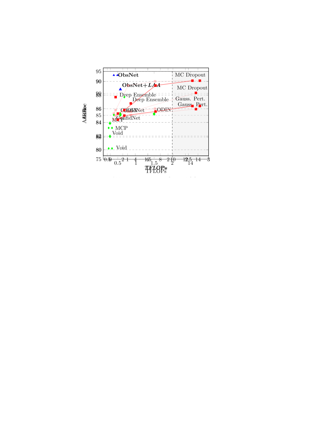
Figure 1: Evaluation of precision vs. test-time computational cost on CamVid OOD. Existing methods for OOD detection in semantic segmentation are either accurate but slow (e.g., MC Dropout [17], Deep Ensemble [30]) or fast but inaccurate (e.g., Maximum Class Prediction [25]). In contrast, our method ObsNet+LAA is both accurate and fast. Additional baselines and evaluation datasets are available in §4.3.

1 Introduction

For real-world decision systems such as autonomous vehicles, accuracy is not the only performance requirement and it often comes second to reliability, robustness, and safety concerns [40], as any failure carries serious consequences. Component modules of such systems frequently rely on Deep Neural Networks (DNNs) which have emerged as a dominating approach across numerous tasks and benchmarks [59, 21, 20]. Yet, a major source of concern is related to the data-driven nature of DNNs as they do not always generalize to objects unseen in the training data. Simple uncertainty estimation techniques, e.g., entropy of softmax predictions [11], are less effective since modern DNNs are consistently overconfident on both in-domain [19] and out-of-distribution (OOD) data samples [46, 25, 23]. This hinders further the performance of downstream components relying on their predictions. Dealing successfully with the “unknown unknown”, e.g., by launching an alert or failing gracefully, is crucial.

In this work we address OOD detection for semantic segmentation, an essential and common task for visual perception in autonomous vehicles. We consider “Out-of-distribution”, pixels from a region that has no training labels associated with. This encompasses unseen objects, but also noise or image alterations. The most effective methods for OOD detection task stem from two major categories of approaches: ensembles and auxiliary error prediction modules. DeepEnsemble (DE) [30] is a prominent and simple ensemble method that exposes potentially unreliable predictions by measuring the disagreement between individual DNNs. In spite of the outstanding performance, DE is computationally demanding for both training and testing and prohibitive for real-time on-vehicle usage. For the latter category, given a trained main task network, a simple model is trained in a second stage to detect its errors or estimate its confidence [10, 22, 4]. Such approaches are computationally lighter, yet, in the context of DNNs, an unexpected drawback is related to the lack of sufficient negative samples, i.e., failures, to properly train the error detector [10]. This is due to an accumulation of causes: reduced size of the training set for this module (essentially a mini validation set to withhold a sufficient amount for training the main predictor), few mistakes made by the main DNNs, hence few negatives.

In this work, we propose to revisit the two-stage approach with modern deep learning tools in a semantic segmentation context. Given the application context, i.e., limited hardware and high performance requirements, we aim for reliable OOD detection (see Figure 1) without compromising on predictive accuracy and computational time. To that end we introduce four design principles aimed at mitigating the most common pitfalls and covering two main aspects, (i) architecture and (ii) training:
(i.a) The pitfall of trading accuracy in the downstream segmentation task for robustness to OOD can be alleviated by decoupling OOD detection from segmentation.
(i.b) Since the processing performed by the segmentation network aims to recognize known objects and is not adapted to OOD objects, the accuracy of the OOD detection can be improved significantly by observing the entire segmentation network instead of just its output.
(ii.a) Training an OOD detector requires additional data that can be generated by leveraging blind spots in the segmentation network.
(ii.b) Generated data should focus on localized regions in the image to mimic unknown objects that are OOD.

Following these principles, we propose a new OOD detection architecture called ObsNet and its associated training scheme based on Local Adversarial Attacks (LAA). We experimentally show that our ObsNet+LAA method achieves top performance in OOD detection on three semantic segmentation datasets (CamVid [9], StreetHazards [24] and BDD-Anomaly [24]), compared to a large set of methods.

Contributions.   To summarize, our contributions are as follows: We propose a new OOD detection method for semantic segmentation based on four design principles: (i.a) decoupling OOD detection from the segmentation task; (i.b) observing the full segmentation network instead of just the output; (ii.a) generating training data for the OOD detector using blind spots of the segmentation network; (ii.b) focusing the adversarial attacks in localized region of the image to simulate unknown objects. We implement these four principles in a new architecture called ObsNet and its associated training scheme using Local Adversarial Attacks (LAA). We perform extensive ablation studies on these principles to validate them empirically. We compare our method to 10 diverse methods from the literature on three datasets (CamVid OOD, StreetHazards, BDD Anomaly) and we show it obtains top performances both in accuracy and in speed.

Strength and weakness.  The strengths and weaknesses of our approach are:

• It can be used with any pre-trained segmentation network without altering their performances and without fine-tuning them (we train only the auxiliary module).

• It is fast since only one extra forward pass is required.

• It is very effective since we show it performs best compared to 10 very diverse methods from the literature on three different datasets.

• The pre-trained segmentation network has to allow for adversarial attacks, which is the case of commonly used deep neural networks.

• Our observer network has a memory/computation overhead equivalent to that of the segmentation network, which is not ideal for real time applications, but far less than that of MC Dropout or deep ensemble methods.

In the next section, we position our work with respect to the existing literature.

2 Related work

Type	Example	OOD accuracy	Fast Inference	Memory efficient	Training specification
Softmax	MCP [25]	-	✓	✓	No
Bayesian Learning	MC Dropout [17]	✓	-	✓	Reduces IoU acc.
Reconstruction	GAN [63]	✓	✓	✓	Unstable training
Ensemble	DeepEnsemble [30]	✓	-	-	Costly Training
Auxiliary Network	ConfidNet [10]	-	✓	✓	Imbalanced train set
Test Time attacks	ODIN [32]	-*	-	✓	Extra OOD set
Prior Networks	Dirichlet [39]	✓	✓	✓	Extra OOD set
Observer	ObsNet + LAA	✓	✓	✓	No

Table 1: Summary of various OOD detection approaches amenable to semantic segmentation. For real-time safety, key requirements for an OOD detector are accuracy, speed, easy training and memory efficiency. Our method addresses all requirements. Our LAA is performed only at train time and mitigates the imbalance in the training data for the observer. *Not accurate for semantic segmentation

The problem of data samples outside the original training distribution has been long studied for various applications before the deep learning era, under slightly different names and angles: outlier [8], novelty [55], anomaly [34] and, more recently, OOD detection [25, 27]. In the context of widespread DNN adoption this field has seen a fresh wave of approaches based on input reconstruction [54, 3, 33, 63], predictive uncertainty [17, 29, 39], ensembles [30, 15], adversarial attacks [32, 31], using a void or background class [51, 35] or dataset [5, 27, 39], etc., to name just a few. We outline here only some of the methods directly related to our approach and group them in a comparative summary in Table 1.

Anomaly detection by reconstruction.   In semantic segmentation, anomalies can be detected by training a (usually variational) autoencoder [12, 3, 62] or generative model [54, 33, 63] on in-distribution data. OOD samples are expected to lead to erroneous and less reliable reconstructions as they contain unseen patterns during training. On high resolution and complex urban images, autoencoders under-perform while more sophisticated generative models require large amounts of data to reach robust reconstruction or rich pipelines with re-synthesis and comparison modules.

Bayesian approaches and ensembles.   BNNs [45, 7] can capture predictive uncertainty from distributions learned over network weights, but don’t scale well [14] and approximate solutions are preferred in practice. DE [30] is a highly effective, yet costly approach, that trains an ensemble of DNNs with different initialization seeds. Pseudo-ensemble approaches [16, 37, 15, 41] are a pragmatic alternative to DE that bypass training of multiple networks and generate predictions from different random subsets of neurons [16, 58] or from networks sampled from approximate weight distributions [37, 15, 41]. However they all require multiple forward passes and/or storage of additional networks in memory. Our ObsNet is faster than ensembles as it requires only the equivalent of two forward passes. Some approaches forego ensembling and propose deterministic networks that can output predictive distributions [39, 56, 50, 61]. They typically trade predictive performance over computational efficiency and results can match MC Dropout [17] for uncertainty estimation.

OOD detection via test-time adversarial attacks.   In ODIN, Liang et al. [32] leverage temperature scaling and small adversarial perturbations on the input at test-time to predict in- and out-of-distribution samples. Lee et. al [31] extend this idea with a confidence score based on class-conditional Mahalanobis distance over hidden activation maps. Both approaches work best when train OOD data is available for tuning, yet this does not ensure generalization to other ODD datasets [57]. Contrarily to us, ODIN uses adversarial attack at test time as a method to detect OOD. However, so far this method has not been shown effective for structured output tasks where the test cost is likely to explode, as adversarial perturbations are necessary for each pixel. In contrast, we propose to use adversarial attacks during training as a proxy for OOD training samples, with no additional test time cost.

Learning to predict errors.   Inspired by early approaches from model calibration literature [49, 66, 67, 43, 44], a number of methods propose endowing the task network with an error prediction branch allowing self-assessment of predictive performance. This branch can be trained jointly with the main network [13, 64], however better learning stability and results are achieved with two-stage sequential training [10, 22, 4, 52] Our ObsNet also uses an auxiliary network and is trained in two stages allowing it to learn from the failure modes of the task network. While [10, 22, 4, 52] focus on in-distribution errors, we address OOD detection for which there is no available training data. In contrast with these methods that struggle with the lack of sufficient negative data to learn from, we devise an effective strategy to generate failures that further enable generalization to OOD detection. We redesign both the training procedure and the architecture of the auxiliary network in order to deal with OOD examples, by introducing Local Adversarial Attack ($\operatorname*{LAA}$).

Generic approaches.   Finally we mention a set of mildly related approaches that do not address directly OOD detection, but achieve good performances on this task. In spite of the overconfidence pathological effect, using the maximum class probability from the softmax prediction can be used towards OOD detection [25, 48]. Temperature scaling [19, 49] is a strong post-hoc calibration strategy of the softmax predictions using a dedicated validation set. If predictions are calibrated, OOD samples can be detected by thresholding scores. Pre-training with adversarial attacked images [26] has also been shown to lead to better calibrated predictions and good OOD detection for image classification. We consider these simple, yet effective approaches as baselines in order to validate the utility of our contribution.

3 Proposed Method

Following our analysis of the related work, we base our OOD semantic segmentation method on two categories of aspects: (i) Architecture: OOD detection has to be decoupled from the segmentation prediction to retain maximal accuracy in both the segmentation and OOD task (§3.1); (ii) Training: Training an OOD detector without OOD data is difficult, but can be done nonetheless by generating training data with carefully designed adversarial attacks (§3.2).

Both of these aspects require careful design to work effectively, which we detail in the following. We validate them experimentally in §4.

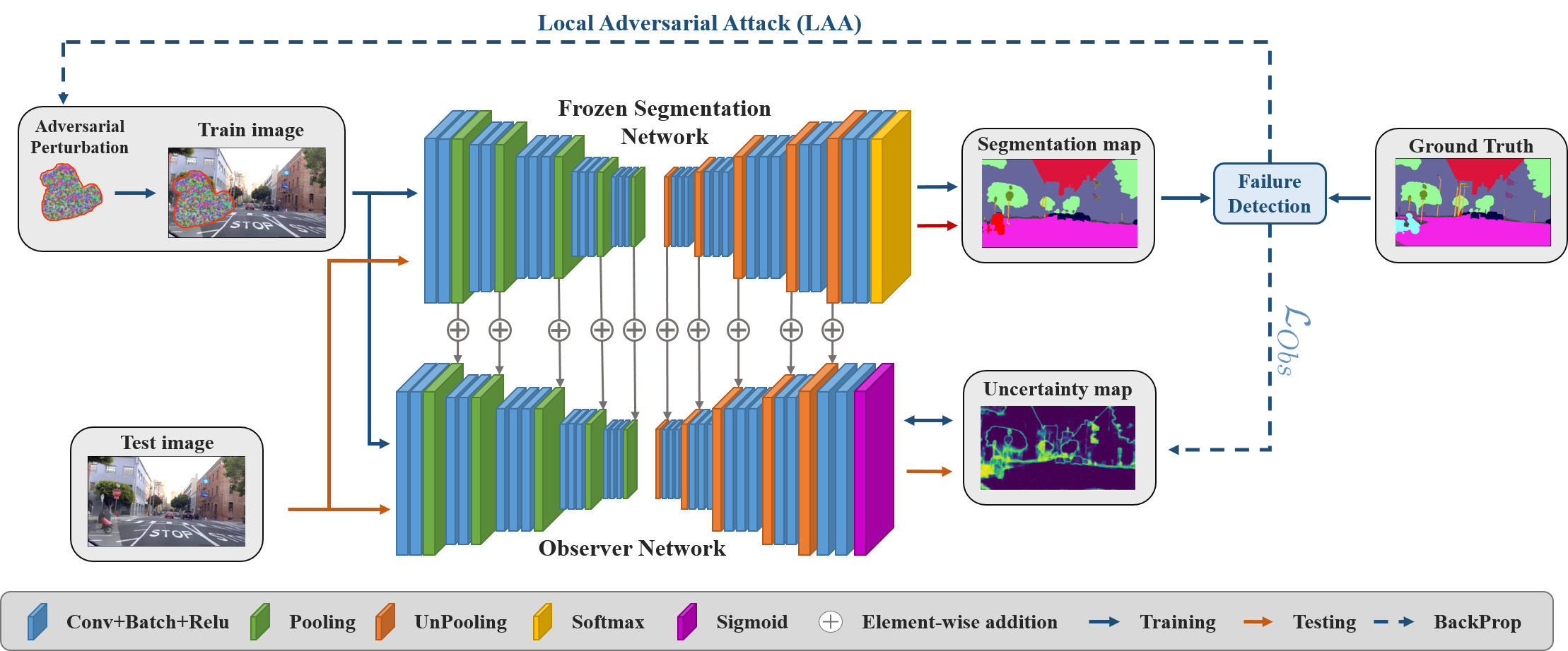
Figure 2: Overview of our method. Training (blue arrow) The Segmentation Network is frozen. The input image is perturbed by a local adversarial attack. Then the Observer Network is trained to predict Segmentation Network’s errors, given the images and some additional skip connections. Testing (red arrow) No augmentation is performed. The Observer Network highlights the out-of-distribution sample, here a motor-cycle. To compute the uncertainty map, the Observer Network requires only one additional forward pass compared to the standard segmentation prediction.

3.1 ObsNet: Dedicated OOD detector

Modifying the segmentation network to account for OOD is expected to impact its accuracy as we show in the experiments. Furthermore, it prevents from using off-the-shelf pretrained segmentation networks that have excellent segmentation accuracy. As such, we follow a two-stage approach where an additional predictor tackles the OOD detection while the segmentation network remains untouched.

In the literature, two-stage approaches are usually related to calibration [49, 66, 67, 43, 44] where the outputs of the segmentation network are mapped to normalized scores. However this is not well adapted for segmentation since it does not use the spatial information contained in nearby predictions. We show in the experiments that using only the output of the segmentation network is not enough to obtain accurate OOD detection.

As such, on the architecture side we follow two design principles in our work:
(i.a) OOD detection should be decoupled from the segmentation prediction to avoid any negative impact on the accuracy of the segmentation task.
(i.b) The OOD detector should observe the full segmentation network instead of just the output.

We thus design an observer network called ObsNet that has a similar architecture to that of the segmentation network and attend the input, the output and intermediate feature maps of the segmentation network as shown on Figure 2. We show experimentally that these design choices lead to increased OOD detection accuracy (see §4.2).

More formally, the observer network (denoted $Obs$) is trained to predict the probability that the segmentation network (denoted $Seg$) output is not aligned with the correct class $y$:

$$Obs(\bm{x},Seg_{r}(\bm{x}))\approx Pr[Seg(\bm{x})\neq y],$$ (1)

where $\bm{x}$ is the input image and $Seg_{r}$ the skip connections from intermediate feature maps of $Seg$.

To that end, we train the ObsNet to minimize a binary cross-entropy loss function:

$$\mathcal{L}_{Obs}(\bm{x},y)=(\mathds{1}_{Seg(\bm{x})\neq y}-1)\log(1-Obs(\bm{x},Seg_{r}(\bm{x})))\\ -\mathds{1}_{Seg(\bm{x})\neq y}\log Obs(\bm{x},Seg_{r}(\bm{x}))$$ (2)

with $\mathds{1}_{Seg(\bm{x})\neq y}$ the indicator function of $Seg(\bm{x})\neq y$.

Discussion.   Since the observer network processes both the image and skip connections from the segmentation network, it has the ability to observe internal behaviour and dynamics of $Seg$ which has been shown to be different when processing an OOD samples (as measured by, e.g., Mahalanobis distance on feature maps [31] or higher order Gram matrices on feature maps [53]).

We emphasize an advantage of our approach w.r.t. previous methods that is related to the low computational complexity, as we only have to make a single forward pass through the segmentation network and the observer network. Experimentally, ObsNet is 21 times faster than MC Dropout with 50 forward passes on a GeForce RTX 2080 Ti, while outperforming it (see §4). Moreover, our method can be readily used on state of the art pre-trained networks without requiring retraining or even fine-tuning them.

3.2 Training ObsNet by triggering Failures

Without a dedicated training set of labeled OOD samples, one could argue that ObsNet is an error detector (similarly to [10]) rather than an OOD detector and that it is furthermore very difficult to train since pre-trained segmentation networks are likely to make few errors. We propose to solve both of these issues by following two design principles:
(ii.a) The lack of training data should be tackled by generating training samples that trigger failures of the segmentation network, which we can obtain using adversarial attacks.
(ii.b) Adversarial attacks should be localized in space since OOD detection in a segmentation context corresponds to unknown objects.

We propose to generate the additional data required to train our ObsNet architecture by performing Local Adversarial Attacks ($\operatorname*{LAA}$) on the input image. In practice, we select a region in the image by using a random shape and we perform a Fast Gradient Sign Method (FSGM) [18] attack such that it is incorrectly classified by the segmentation network:

$$\tilde{\bm{x}} =\bm{x}+\operatorname*{LAA}(Seg,\bm{x})$$ (3)

$$\operatorname*{LAA}(Seg,\bm{x}) =\epsilon\operatorname{sign}(\nabla_{\bm{x}}\mathcal{L}(Seg(\bm{x}),y))\Omega(\bm{x})$$ (4)

with step $\epsilon$, $\mathcal{L}(\cdot)$ the categorical cross entropy and $\Omega(\bm{x})$ the binary mask of the random shape. We show $\operatorname*{LAA}$ examples in Figure 3 and schematize the training process in Figure 2.

The reasoning behind $\operatorname*{LAA}$ is two-fold. First, by controlling the shape of the attack, we can make sure that the generated example does not accidentally belong to the distribution of the training set. Second, leveraging adversarial attacks allows us to focus the training just beyond the boundaries of the predicted classes which tend to be far from the training data due to the high capacity and overconfidence of DNNs, like OOD objects would be.

We show in the experiments that $\operatorname*{LAA}$ produces a good training set for learning to detect OOD examples. In practice, we found that generating random shapes is essential to obtain good performances in contrast to non-local adversarial attacks. These random shapes coupled with $\operatorname*{LAA}$ may mimic unknown objects or objects parts, exposing common behavior patterns in the segmentation network when facing them. We validate our approach in an ablation study in §4.2.

Discussion.   We point out that by triggering failures using $\operatorname*{LAA}$, we address the problem of the low error rates of the segmentation network. We can in fact generate as many OOD-like examples as needed to balance the positive (i.e., correct predictions) and negative (i.e., erroneous predictions) terms in Equation 2 for training the observer network. Thus, even if the segmentation network attains nearly perfect performances on the training set, we are still able to train the ObsNet to detect where the predictions of the segmentation network are unreliable.

One could ask why not using $\operatorname*{LAA}$ for training a more robust and reliable segmentation network in the first place, as done in previous works [18, 42, 26], instead of adding and training the observer network. Training with adversarial examples improves the robustness of the segmentation network at the cost of its accuracy (See §4.2), but it will not make it infallible as there will still be numerous blind-spots in the multi-million dimensional parameter space of the network. It also prevents from using pre-trained state-of-the-art segmentation networks. Here, we are rather interested in capturing the main failure modes of the segmentation network to enable ObsNet to learn and to recognize them later on OOD objects.

Finally, one could ask why not perform adversarial attacks at test time as it is done in ODIN [32]. Performing test time attacks has two major drawbacks. First it is computationally intensive at test time since it requires numerous backward passes, i.e., one attack per pixel. Second, it is not well adapted to segmentation as perturbations of a single pixels can have effect on a large areas (e.g., one pixel attacks) thus hindering the detection accuracy of perfectly valid predictions. We show in §4.3 that our training scheme is better performing both in accuracy and speed when compared to test time attacks.

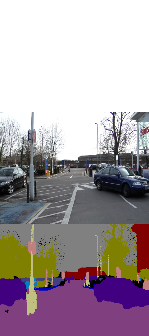
(a) No attack

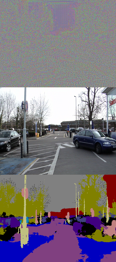
(b) All pixels

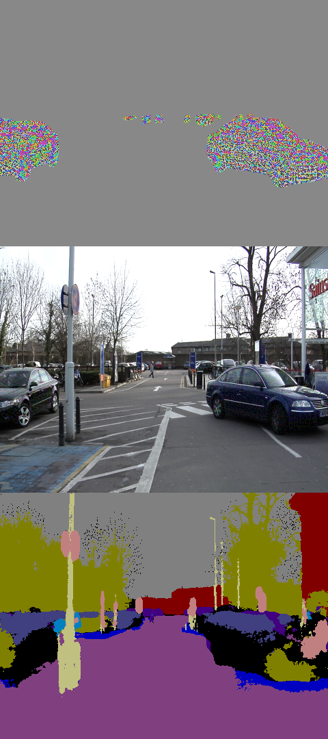
(c) Class wise

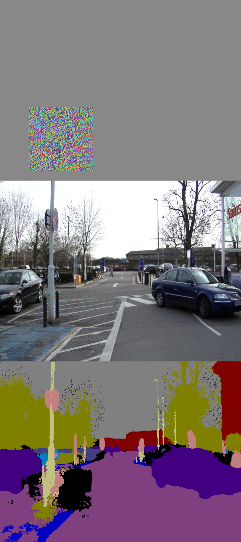
(d) Square shape

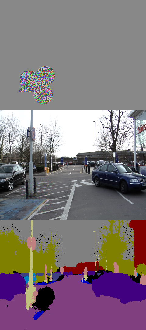
(e) Random shape

Figure 3: Adversarial attack examples. Top: Perturbations magnified 25$\times$; middle: Input image with attacks; bottom: SegNet prediction.

4 Experiments

In this section, we present extensive experiments to validate that our proposed observer network combined with local adversarial attacks outperforms a large set of very different methods on three different benchmarks.

4.1 Datasets & Metrics

To highlight our results, we select three datasets for Semantic Segmentation of urban streets scenes with anomalies in the test set. Anomalies correspond to out-of-distribution objects, not seen during train time.

CamVid OOD: We design a custom version of CamVid [9], where we blit random animals from [36] in a random part of the image. This dataset contains $367$ train and $233$ test images. There are $19$ different species of animals, and one animal in each test image. This setup is analog to that of Fishyscapes [6], with the main advantage that it does not require the use of an external evaluation server and that we provide a wide variety of baselines.

StreetHazards: This is a synthetic dataset [24] from the Carla simulator. It is composed of $5125$ train and $1500$ test images, collected in six virtual towns. There are $250$ different kinds of anomalies (like UFO, dinosaur, helicopter, etc.) with at least one anomaly per image.

BDD Anomaly: Composed of real images, this dataset is sourced from the BDD100K semantic segmentation dataset [65]. Here, motor-cycle and train are selected as anomalous objects and all images containing these objects are removed from the training set. The remaining dataset contains $6688$ images for training and $361$ for testing.

To evaluate each method on these datasets, we select three metrics for detecting misclassified and out-of-distribution examples and one metric for calibration:

• fpr95tpr [32]: It measures the false positive rate when the true positive rate is equal to 95%. The aim is to obtain the lowest possible false positive rate while guaranteeing a given number of detected errors.

• Area Under the Receiver Operating Characteristic curve (AuRoc) [25]: This threshold free metric corresponds to the probability that a certain example has a higher value than an uncertain one.

• Area under the Precision-Recall Curve (AuPR) [25]: Also a threshold-independent metric. The AuPR is less sensitive to unbalanced dataset than AuRoc.

• Adaptive Calibration Error (ACE) [47]: Compared to standard calibration metrics where bins are fixed, ACE adapts the range of each the bin to focus more on the region where most of the predictions are made.

For all our segmentation experiments we use a Bayesian SegNet [2], [28] as the main network. Therefore, our ObsNet follows the same architecture as this SegNet. Ablation on the architecture of ObsNet, hyper-parameters and training details can be found in the supplementary material.

4.2 Ablation Study

First, to validate that the local adversarial attack contributes to improving the observer network, we show on Table 2 the performance gap for each metric on each dataset. This validates the use of LAA to train the observer network as per principle (ii.a).

Dataset	Adv	fpr95tpr $\downarrow$	AuPR $\uparrow$	AuRoc $\uparrow$
CamVid OOD	✗	54.2	97.1	89.1
	✓	44.6	97.6	90.9
StreetHazards	✗	50.1	98.3	89.7
	✓	44.7	98.9	92.7
BDD Anomaly	✗	62.4	95.9	81.7
	✓	60.3	96.2	82.8

Table 2: Evaluation of the Local Adversarial Attack on each dataset.

The $\operatorname*{LAA}$ can be seen as a data augmentation performed during ObsNet training. We emphasize that this type of data augmentation is not beneficial for the main network training, which is known as robust training [38], and that it requires an external observer network. Indeed, Table 3 illustrates the drop of accuracy when training the main network with the same adversarial augmentation as there is a trade-off between the accuracy and the robustness of a deep neural network [60]. In contrast, our method keeps the main network frozen during ObsNet training, thus, the class prediction and the accuracy remain unchanged, validating principle (i.a).

Dataset	Robust	Mean IoU $\uparrow$	Global Acc $\uparrow$
Camvid ODD	-	49.6	81.8
	✓	41.6	73.9
StreetHazards	-	44.3	87.9
	✓	37.8	85.1
Bdd Anomaly	-	42.9	87.0
	✓	41.5	85.9

Table 3: Impact of robust training on accuracy.

In Table 4, we show ablations on $\operatorname*{LAA}$ by varying the type of noise (varying between attacking all pixels, random pixels, pixels from a specific class, pixels inside a square shape and pixels inside a random shape, see Figure 3). We conclude that local attacks on random shaped regions produce the best proxies for OOD detection (see supplementary material for detailed results), validating principle (ii.b).

Type	fpr95tpr $\downarrow$	AuPR $\uparrow$	AuRoc $\uparrow$
All pixels	51.9	97.1	89.6
Sparse pixels	54.2	97.2	89.6
Class pixels	46.8	97.2	89.9
Square patch	45.5	97.4	90.5
Random shape	44.6	97.4	90.6

Table 4: LAA ablation study by varying the attacked region.

In Table 5, we conduct several ablation studies on the architecture of ObsNet. The main takeaway is that mimicking the architecture of the primary network and adding skip connections from several intermediate feature maps is essential to obtain the best performances (see full results in supplementary material), validating principle (i.b).

Method	fpr95tpr $\downarrow$	AuPR $\uparrow$	AuRoc $\uparrow$
Smaller architecture	60.3	95.8	85.3
ObsNet w/o skip	81.3	92.0	74.4
ObsNet w/o input image	57.0	96.9	88.2
ObsNet	54.2	97.1	89.1

Table 5: ObsNet architecture ablation study.

4.3 Quantitative and Qualitative results

We report results on Table 6, Table 7 and Table 8, with all the metrics detailed above. We compare several methods:

• MCP [25]: Maximum Class Prediction. One minus the maximum of the prediction.

• AE [25]: An autoencoder baseline. The reconstruction error is the uncertainty measurement.

• Void [6]: Void/background class prediction of the segmentation network.

• MCDA [1]: Data augmentation such as geometric and color transformations is added during inference time. We use the entropy of 25 forward passes.

• MC Dropout [17]: The entropy of the mean softmax prediction with dropout. We use 50 forward passes for all the experiences.

• Gaussian Perturbation Ensemble [15, 41]: We take a pre-trained network and perturb its weights with a random Normal distribution. This results in an ensemble of networks centered around the pre-trained model.

• ConfidNet [10]: ConfidNet is an observer network that is trained to predict the true class score. We use the code available online and modify the data loader to test ConfidNet on our experimental setup.

• Temperature Scaling [19]: We chose the hyper-parameters Temp to have the best calibration on the validation set. Then, like MCP, we use one minus the maximum of the scaled prediction.

• ODIN [32]: ODIN performs test-time adversarial attacks on the primary network. We seek the hyper-parameters Temp and $\epsilon$ to have the best performance on the validation set. The criterion is one minus the maximum prediction.

• Deep ensemble [30]: a small ensemble of 3 networks. We use the entropy the averaged forward passes.

As we can see on these tables, ObsNet significantly outperforms all other methods on detection metrics on all three datasets. Furthermore, ACE also shows that we succeed in having a good calibration value.

Method	fpr95tpr$\downarrow$	AuPR $\uparrow$	AuRoc $\uparrow$	ACE $\downarrow$
Softmax [25]	65.4	94.9	83.2	0.510
Void [6]	66.6	93.9	80.2	0.532
AE [25]	93.0	87.1	59.3	0.745
MCDA [1]	66.5	94.6	82.1	0.477
Temp. Scale [19]	63.8	94.9	83.7	0.356
ODIN [32]	60.0	95.4	85.3	0.500
ConfidNet [10]	60.9	96.2	85.1	0.450
Gauss Pert. [15, 41]	59.2	96.0	86.4	0.520
Deep Ensemble [30]	56.2	96.6	87.7	0.459
MC Dropout [17]	49.3	97.3	90.1	0.463
ObsNet + LAA	44.6	97.6	90.9	0.446

Table 6: Evaluation on CamVid-ODD (best method in bold, second best underlined).

Method	fpr95tpr $\downarrow$	AuPR $\uparrow$	AuRoc $\uparrow$	ACE $\downarrow$
Softmax [25]	65.5	94.7	80.8	0.463
Void [6]	69.3	93.6	73.5	0.492
AE [25]	84.6	92.7	67.3	0.712
MCDA [1]	69.9	97.1	82.7	0.409
Temp. Scale [19]	65.3	94.9	81.6	0.323
ODIN [32]	61.3	95.0	82.3	0.414
ConfidNet [10]	60.1	98.1	90.3	0.399
Gauss Pert. [15, 41]	48.7	98.5	90.7	0.449
Deep Ensemble [30]	51.7	98.3	88.9	0.437
MC Dropout [17]	45.7	98.8	92.2	0.429
ObsNet + LAA	44.7	98.9	92.7	0.383

Table 7: Evaluation on StreetHazard (best method in bold, second best underlined).

Method	fpr95tpr $\downarrow$	AuPR $\uparrow$	AuRoc $\uparrow$	ACE $\downarrow$
Softmax [25]	63.5	95.4	80.1	0.633
Void [6]	68.1	92.4	75.3	0.499
AE [25]	92.1	88.0	53.1	0.832
MCDA [1]	61.9	95.8	82.0	0.411
Temp. Scale [19]	61.8	95.8	81.9	0.287
ODIN [32]	60.6	95.7	81.7	0.353
ConfidNet [10]	61.6	95.9	81.9	0.367
Gauss Pert. [15, 41]	61.3	96.0	82.5	0.384
Deep Ensemble [30]	60.3	96.1	82.3	0.375
MC Dropout [17]	61.1	96.0	82.6	0.394
ObsNet + LAA	60.3	96.2	82.8	0.345

Table 8: Evaluation on Bdd Anomaly (best method in bold, second best underlined).

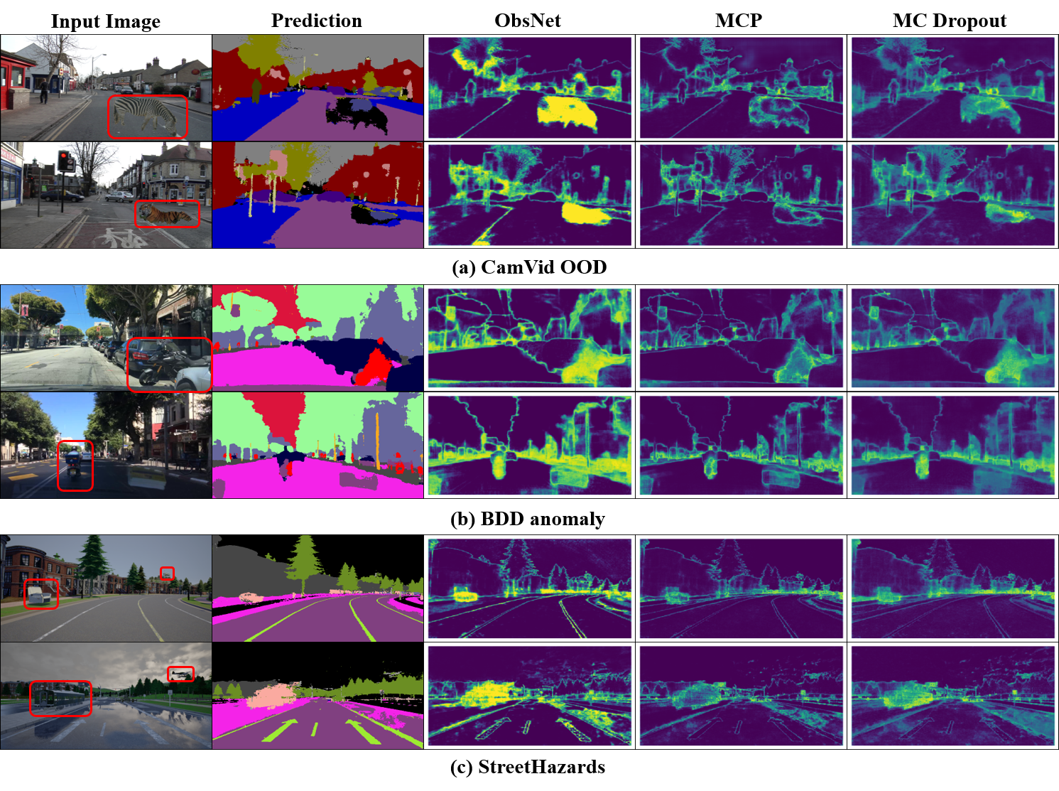
Figure 4: Uncertainty map visualization. 1st column: We highlight the ground truth locations of the OOD objects to help visualize them (red bounding box). 2nd column: Segmentation map of the SegNet. 3rd to 5th columns: Uncertainty Map highlight in yellow. Our method produces stronger responses on OOD regions compared to other methods, while being as strong on regular error regions, e.g., boundaries

To show where the uncertainty is localized, we outline the uncertainty map on the test set (see Figure 4). We can see that our method is not only able to correctly detect OOD objects, but also to highlight areas where the predictions are wrong (edges, small and far objects, etc).

Finally, the trade-off between accuracy and speed is shown on Figure 1, where we obtain excellent accuracy without any compromise over speed.

5 Conclusion

In this paper, we propose an observer network called ObsNet to address OOD detection in semantic segmentation, by learning from triggered failures. We use skip connection to allow the observer network to seek abnormal behaviour inside the main network. We use local adversarial attacks to trigger failures in the segmentation network and train the observer network on these samples. We show on three different segmentation datasets that our strategy combining an observer network with local adversarial attacks is fast, accurate and is able to detect unknown objects.

1 Implementation details & hyper-parameters

For our implementation, we use Pytorch and will release the code after the review. We share each hyper-parameter in Table 9. We train ObsNet with SGD with momentum and weight decay for at most $50$ epochs using early-stopping. ObsNet is not trained from scratch as we initialize the weights with those of the segmentation network. We also use a scheduler to divide the learning rate by 2 at epoch 25 and epoch 45. We use the same data augmentation (i.e. Horizontal Flip and Random Crop) for training of the segmentation network and as well as for ObsNet. As there are few errors in the training of ObsNet, we increase the weight of positive examples in the loss contribution (Pos Weight in Table 9).

Params	CamVid	StreetHazards	Bdd Anomaly
Epoch	50	50	50
Optimizer	SGD	SGD	SGD
LR	0.05	0.02	0.02
Batch Size	8	6	6
Loss	BCE	BCE	BCE
Pos Weight	2	3	3
LAA shape	rand shape	rand shape	rand shape
LAA type	$\min_{p(c)}$	$\max_{p(k\neq c)}$	$\max_{p(k\neq c)}$
epsilon	0.02	0.001	0.001

Table 9: Hyper-parameters to train ObsNet on the different datasets.

	Type	fpr95tpr $\downarrow$	AuPR $\uparrow$	AuRoc $\uparrow$	ACE $\downarrow$
	MC Dropout	49.3	97.3	90.1	0.463
	ObsNet base	54.2	97.1	89.1	0.396
	all pixels	53.2	97.1	89.5	0.410
	sparse pixels	61.1	97.1	89.2	0.387
$\min_{p(c)}$	class pixels	45.6	97.3	90.3	0.428
	square patch	47.4	97.3	90.1	0.461
	rand shape	44.6	97.6	90.9	0.446
	all pixels	51.9	97.1	89.6	0.405
	sparse pixels	54.2	97.2	89.6	0.374
$\max_{p(k\neq c)}$	class pixels	46.8	97.2	89.9	0.432
	square patch	45.5	97.4	90.5	0.464
	rand shape	44.6	97.4	90.6	0.446

Table 10: Ablation on adversarial attacks.

2 Ablation on ObsNet architecture, $\epsilon$ and $\operatorname*{LAA}$

One contribution of our work is the ablation we do on the architecture of the observer network compared to previous methods. We highlight that the skip connections are essential for reaching best performance. For the smaller architecture, instead of keeping the same architecture as the segmentation network, we design a smaller variant: a convolutional network with three convolutional layers and a fully connected layer. This architecture mimicks the one used by ConfidNet [10].

Method	fpr95tpr $\downarrow$	AuPR $\uparrow$	AuRoc $\uparrow$	ACE $\downarrow$
Smaller archi.	60.3	95.8	85.3	0.476
w/o skip	81.3	92.0	74.4	0.551
w/o input img	57.0	96.9	88.2	0.455
w/o pretrain	55.7	96.9	88.7	0.419
ObsNet full	54.2	97.1	89.1	0.396

Table 11: Ablation ObsNet without $\operatorname*{LAA}$ training.

Next, we outline most of the experiments we make on $\operatorname*{LAA}$. First, there are two different kinds of setups, we can either minimize the prediction class (i.e. $\min_{p(c)}$) or maximize instead a different class (i.e. $\max_{p(k\neq c)}$), with $p=Seg(x)$ the class vector, $c=\max_{p}$ the maximum class prediction and $k$ a random class. Then, we attack with five different strategies: all pixels in the image, random sparse pixels, the area of a random class, all pixels in a square patch and all pixels in a random shape. We show in Table 10 the complete results on CamVid ODD. We can see that that random shape is the most effective. We use the FSGM because it’s a well-known and easy-to-use adversarial attack. Since our goal is to hallucinate OOD objects, we believe the location and the shape of the attacked region are the important part.

Method	fpr95tpr $\downarrow$	AuPR $\uparrow$	AuRoc $\uparrow$	ACE $\downarrow$
Softmax [25]	61.9	96.5	84.4	0.480
Void [6]	79.9	90.7	67.3	0.504
MCDA [1]	65.8	96.3	83.1	0.440
Temp. Scale [19]	61.9	96.6	84.6	0.302
ODIN [32]	58.3	97.2	87.9	0.478
ConfidNet [10]	52.2	97.5	88.6	0.412
Gauss Pert. [15,41]	60.2	96.8	85.6	0.497
Deep Ensemble [30]	55.3	97.5	88.1	0.343
MC Dropout [17]	52.5	97.9	88.5	0.443
ObsNet + LAA	47.7	98.1	90.3	0.370

Table 12: Error detection evaluation on CamVid (best method in bold, second best underlined).

As shown on Figure 5, we can see that the best $\epsilon$ for the attack is $0.02$ with a random shape blit at a random position in the image. We can also see that even with a large $\epsilon$, ObsNet still achieves reasonable performance.

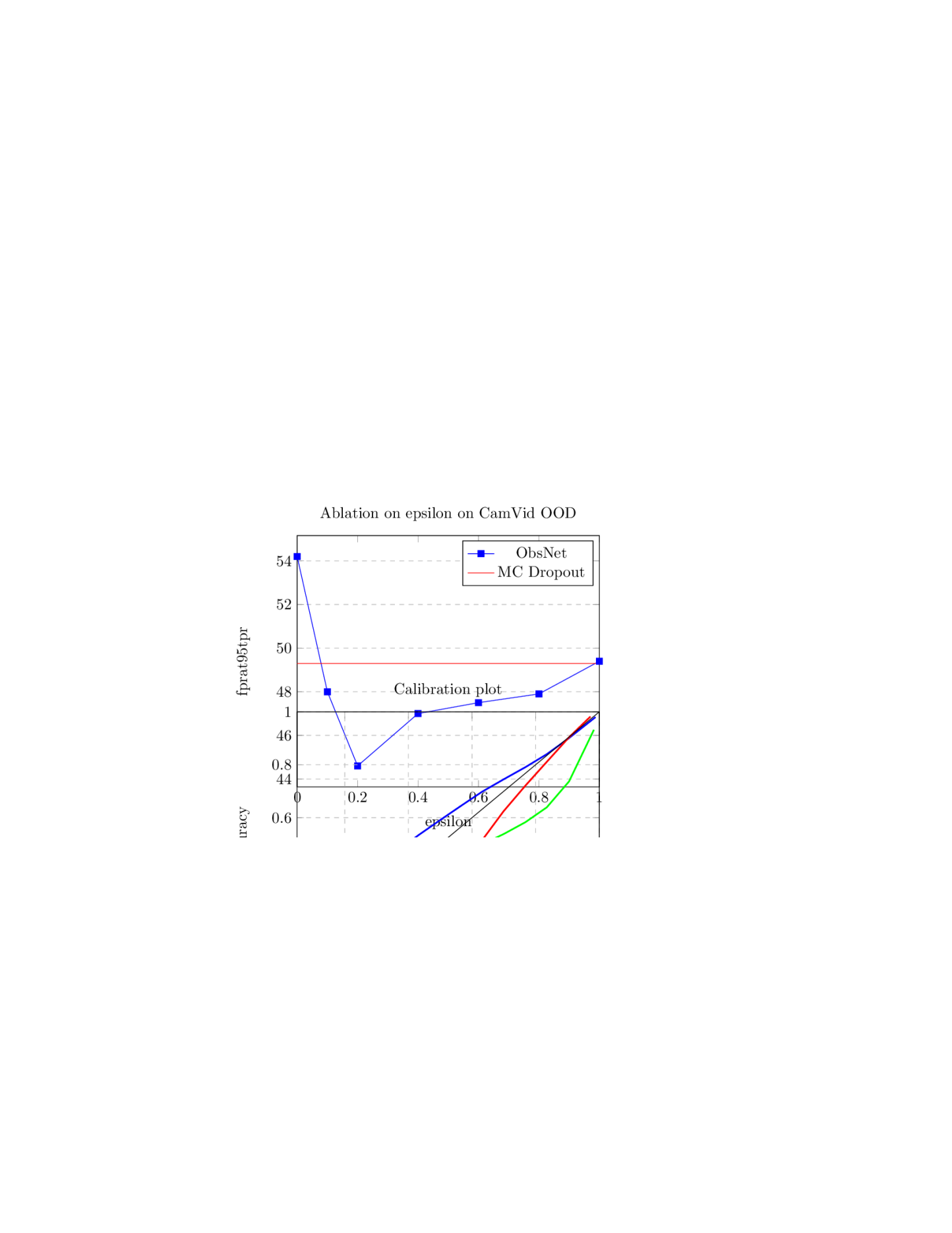
Figure 5: Evolution of the Fpr at 95 Tpr for different values of epsilon on CamVid OOD.

3 Error detector

The observer is trained to assess whether the prediction differs from the true class (which is always the case for OOD regions), so it also tends to assign low confidence scores for in-domain regions with likely high errors, as shown in Figure 6. This behavior is not caused by ObsNet, but depends on the accuracy of the main network at test time and should lessen with more accurate networks. This effect shows that our method can be used for error detection, and outperforms all other methods, as illustrated in Table 12.

4 Additional Experiments: DeepLab v3+

We show on Table 13, the results on BDD Anomaly with a more recent Deeplab v3+ with ResNet-101 encoder. Our methods performs the best, while methods like ConfidNet do not scale when the segmentation accuracy increases as they have fewer errors to learn from.

Method	fpr95tpr $\downarrow$	AuPR $\uparrow$	AuRoc $\uparrow$	ACE $\downarrow$
Softmax [25]	60.3	95.8	81.4	0.228
Void [6]	68.8	90.2	74.0	0.485
MCDA [1]	68.1	95.1	78.8	0.265
ConfidNet [10]	64.5	95.4	80.9	0.254
Gauss Pert. [15,41]	61.4	96.1	82.4	0.186
MC Dropout [17]	60.0	96.0	82.0	0.219
ObsNet + LAA	58.8	96.3	83.0	0.185

Table 13: Evaluation on Bdd Anomaly (best method in bold, second best underlined), with a DeepLab v3+.

5 CamVid OOD dataset

For our experiments, we use urban street segmentation datasets with anomalies withheld during training. Unfortunately, there are few datasets with anomalies in the test set. For this reason we propose the CamVid OOD that will be made public after the review. To design CamVid OOD, we blit random animals in test images of CamVid. We add one different such anomaly in each of the $233$ test images. The rest of the $367$ training images remain unchanged. The anomalous animals are bear, cow, lion, panda, deer, coyote, zebra, skunk, gorilla, giraffe, elephant, goat, leopard, horse, cougar, tiger, sheep, penguin, and kangaroo. Then, we add them to a $13$th class which is animals/anomalies as the corresponding ground truth of the test set.

Method	fpr95tpr $\downarrow$	AuPR $\uparrow$	AuRoc $\uparrow$	ACE $\downarrow$
Softmax [25]	67.5	94.7	82.5	0.529
ConfidNet [10]	58.4	96.4	86.8	0.462
Gauss Pert. [15,41]	61.8	95.8	85.7	0.473
Deep Ensemble [30]	63.9	96.5	86.4	0.468
MC Dropout [17]	52.8	97.2	88.5	0.483
ObsNet + LAA	42.1	97.7	91.4	0.423

Table 14: Error detection evaluation on CamVid with random square attacks (best method in bold).

This setup is similar to the Fishyscape dataset [6], without the constraint of sending a Tensorflow model online for evaluation. Thus, our dataset is easier to work with. We present some examples of the anomalies in Figure 7 with the ground truth highlighted in cyan.

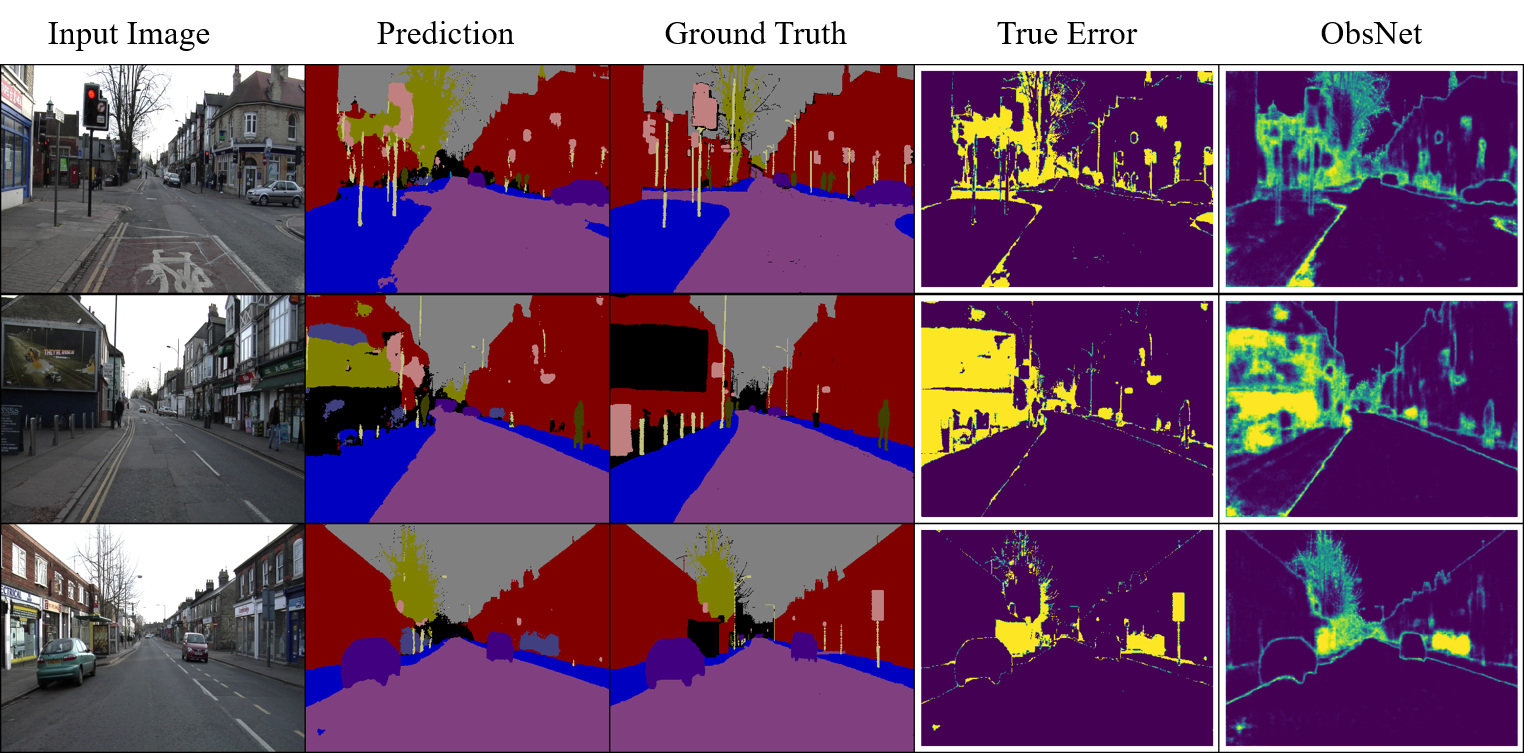
Figure 6: Evaluation of the error detection on the test set of CamVid. ObsNet prediction is close to real errors even without OOD objects.

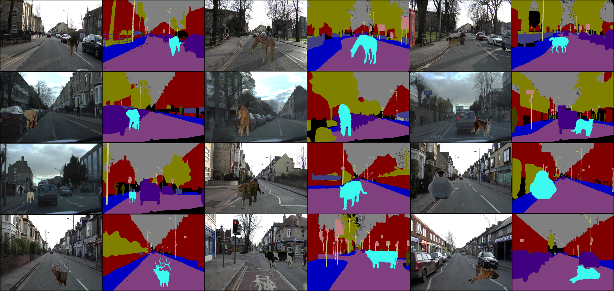
Figure 7: Examples of our dataset with anomalies and the ground truth.

6 Adversarial Attacks Detector

In safety-critical applications like autonomous driving, we know that the perception system has to be robust to adversarial attacks. Nevertheless, training a robust network is costly and robustness comes with a certain trade-off to make between accuracy and run time. Moreover, the task to only detect the adversarial attack could be sufficient as we can rely on other sensors (LiDAR, Radar, etc.). Although, in this work we do not focus on Adversarial Robustness, empirically we note that ObsNet can detect an attack. To some extent this is expected as we explicitly train the observer to detect adversarial attacks, thanks to the $\operatorname*{LAA}$.

Indeed, our observer can detect the area where the attack is performed, whereas the MC Dropout is overconfident. Furthermore, in Table 14, we evaluate the adversarial attack detection of several methods. We apply a FGSM attack in a local square patch on each testing image. Once again, we can see that our observer is the best method to capture the perturbed area.

References

- [1] Murat Seçkin Ayhan and Philipp Berens. Test-time data augmentation for estimation of heteroscedastic aleatoric uncertainty in deep neural networks. Medical Imaging with Deep Learning, 2018.
- [2] Vijay Badrinarayanan, Alex Kendall, and Roberto Cipolla. Segnet: A deep convolutional encoder-decoder architecture for image segmentation. IEEE Trans. PAMI, 2017.
- [3] Christoph Baur, Benedikt Wiestler, Shadi Albarqouni, and Nassir Navab. Deep autoencoding models for unsupervised anomaly segmentation in brain mr images. In International MICCAI Brainlesion Workshop, pages 161–169. Springer, 2018.
- [4] Victor Besnier, David Picard, and Alexandre Briot. Learning uncertainty for safety-oriented semantic segmentation in autonomous driving. arXiv preprint arXiv:2105.13688, 2021.
- [5] Petra Bevandić, Ivan Krešo, Marin Oršić, and Siniša Šegvić. Simultaneous semantic segmentation and outlier detection in presence of domain shift. In GCPR, 2019.
- [6] Hermann Blum, Paul-Edouard Sarlin, Juan Nieto, Roland Siegwart, and Cesar Cadena. The fishyscapes benchmark: Measuring blind spots in semantic segmentation. arXiv, 2019.
- [7] Charles Blundell, Julien Cornebise, Koray Kavukcuoglu, and Daan Wierstra. Weight uncertainty in neural networks. ICML, 2015.
- [8] Markus M Breunig, Hans-Peter Kriegel, Raymond T Ng, and Jörg Sander. Lof: identifying density-based local outliers. In Proceedings of the 2000 ACM SIGMOD international conference on Management of data, pages 93–104, 2000.
- [9] Gabriel J. Brostow, Julien Fauqueur, and Roberto Cipolla. Semantic object classes in video: A high-definition ground truth database. Pattern Recognition Letters, 2008.
- [10] Charles Corbière, Nicolas Thome, Avner Bar-Hen, Matthieu Cord, and Patrick Pérez. Addressing failure prediction by learning model confidence. In NeurIPS, 2019.
- [11] Thomas M Cover. Elements of information theory. John Wiley & Sons, 1999.
- [12] Clement Creusot and Asim Munawar. Real-time small obstacle detection on highways using compressive rbm road reconstruction. In 2015 IEEE Intelligent Vehicles Symposium (IV), pages 162–167. IEEE, 2015.
- [13] Terrance DeVries and Graham W Taylor. Learning confidence for out-of-distribution detection in neural networks. arXiv, 2018.
- [14] Michael W. Dusenberry, Ghassen Jerfel, Yeming Wen, Yian Ma, Jasper Snoek, Katherine Heller, Balaji Lakshminarayanan, and Dustin Tran. Efficient and scalable bayesian neural nets with rank-1 factors. In ICML, 2020.
- [15] Gianni Franchi, Andrei Bursuc, Emanuel Aldea, Séverine Dubuisson, and Isabelle Bloch. Tradi: Tracking deep neural network weight distributions. In ECCV, 2020.
- [16] Yarin Gal. Uncertainty in Deep Learning. PhD, 2016.
- [17] Yarin Gal and Zoubin Ghahramani. Dropout as a bayesian approximation: Representing model uncertainty in deep learning. In ICML, 2016.
- [18] Ian J. Goodfellow, Jonathon Shlens, and Christian Szegedy. Explaining and harnessing adversarial examples. ICLR, 2015.
- [19] Chuan Guo, Geoff Pleiss, Yu Sun, and Kilian Q. Weinberger. On calibration of modern neural networks. ICML, 2017.
- [20] Kaiming He, Georgia Gkioxari, Piotr Dollár, and Ross Girshick. Mask R-CNN. In ICCV, 2017.
- [21] Kaiming He, Xiangyu Zhang, Shaoqing Ren, and Jian Sun. Deep residual learning for image recognition. In CVPR, 2016.
- [22] Simon Hecker, Dengxin Dai, and Luc Van Gool. Failure prediction for autonomous driving. In 2018 IEEE Intelligent Vehicles Symposium (IV), pages 1792–1799. IEEE, 2018.
- [23] Matthias Hein, Maksym Andriushchenko, and Julian Bitterwolf. Why relu networks yield high-confidence predictions far away from the training data and how to mitigate the problem. In CVPR, 2019.
- [24] Dan Hendrycks, Steven Basart, Mantas Mazeika, Mohammadreza Mostajabi, Jacob Steinhardt, and Dawn Song. A benchmark for anomaly segmentation. ArXiv, 2019.
- [25] Dan Hendrycks and Kevin Gimpel. A baseline for detecting misclassified and out-of-distribution examples in neural networks. In ICLR, 2017.
- [26] Dan Hendrycks, Kimin Lee, and Mantas Mazeika. Using pre-training can improve model robustness and uncertainty. In ICML, 2019.
- [27] Dan Hendrycks, Mantas Mazeika, and Thomas Dietterich. Deep anomaly detection with outlier exposure. arXiv, 2018.
- [28] Alex Kendall, Vijay Badrinarayanan, , and Roberto Cipolla. Bayesian segnet: Model uncertainty in deep convolutional encoder-decoder architectures for scene understanding. arXiv, 2015.
- [29] Alex Kendall and Yarin Gal. What uncertainties do we need in bayesian deep learning for computer vision? In NeurIPS, 2017.
- [30] Balaji Lakshminarayanan, Alexander Pritzel, and Charles Blundell. Simple and scalable predictive uncertainty estimation using deep ensembles. In NeurIPS, 2017.
- [31] Kimin Lee, Kibok Lee, Honglak Lee, and Jinwoo Shin. A simple unified framework for detecting out-of-distribution samples and adversarial attacks. In NeurIPS, 2018.
- [32] Shiyu Liang, R. Srikant, and Yixuan Li. Enhancing the reliability of out-of-distribution image detection in neural networks. In ICLR, 2018.
- [33] Krzysztof Lis, Krishna Nakka, Pascal Fua, and Mathieu Salzmann. Detecting the unexpected via image resynthesis. In ICCV, 2019.
- [34] Fei Tony Liu, Kai Ming Ting, and Zhi-Hua Zhou. Isolation forest. In KDD, 2008.
- [35] Wei Liu, Dragomir Anguelov, Dumitru Erhan, Christian Szegedy, Scott Reed, Cheng-Yang Fu, and Alexander C Berg. Ssd: Single shot multibox detector. In ECCV, 2016.
- [36] Heydar Maboudi Afkham, Alireza Tavakoli Targhi, Jan-Olof Eklundh, and Andrzej Pronobis. Joint visual vocabulary for animal classification. In ICPR, 2008.
- [37] Wesley J Maddox, Pavel Izmailov, Timur Garipov, Dmitry P Vetrov, and Andrew Gordon Wilson. A simple baseline for bayesian uncertainty in deep learning. In NeurIPS, 2019.
- [38] Aleksander Madry, Aleksandar Makelov, Ludwig Schmidt, Dimitris Tsipras, and Adrian Vladu. Towards deep learning models resistant to adversarial attacks. In ICLR, 2018.
- [39] Andrey Malinin and Mark Gales. Predictive uncertainty estimation via prior networks. In NeurIPS, 2018.
- [40] Rowan McAllister, Yarin Gal, Alex Kendall, Mark Van Der Wilk, Amar Shah, Roberto Cipolla, and Adrian Weller. Concrete problems for autonomous vehicle safety: Advantages of bayesian deep learning. IJCAI, 2017.
- [41] Alireza Mehrtash, Purang Abolmaesumi, Polina Golland, Tina Kapur, Demian Wassermann, and William M Wells III. Pep: Parameter ensembling by perturbation. In NeurIPS, 2020.
- [42] Takeru Miyato, Shin-ichi Maeda, Masanori Koyama, and Shin Ishii. Virtual adversarial training: a regularization method for supervised and semi-supervised learning. IEEE Trans. PAMI, 2018.
- [43] Mahdi Pakdaman Naeini, Gregory Cooper, and Milos Hauskrecht. Obtaining well calibrated probabilities using bayesian binning. In AAAI, 2015.
- [44] Mahdi Pakdaman Naeini and Gregory F Cooper. Binary classifier calibration using an ensemble of near isotonic regression models. In KDD, 2016.
- [45] Radford M Neal. Bayesian learning for neural networks, volume 118. Springer Science & Business Media, 2012.
- [46] A. Nguyen, J. Yosinski, and J. Clune. Deep neural networks are easily fooled: High confidence predictions for unrecognizable images. In CVPR, 2015.
- [47] Jeremy Nixon, Michael W. Dusenberry, Linchuan Zhang, Ghassen Jerfel, and Dustin Tran. Measuring calibration in deep learning. In CVPRW, 2019.
- [48] Philipp Oberdiek, Matthias Rottmann, and Gernot A. Fink. Detection and retrieval of out-of-distribution objects in semantic segmentation. In Proceedings of the IEEE/CVF Conference on Computer Vision and Pattern Recognition (CVPR) Workshops, June 2020.
- [49] John Platt et al. Probabilistic outputs for support vector machines and comparisons to regularized likelihood methods. Advances in large margin classifiers, 10(3):61–74, 1999.
- [50] Janis Postels, Francesco Ferroni, Huseyin Coskun, Nassir Navab, and Federico Tombari. Sampling-free epistemic uncertainty estimation using approximated variance propagation. In ICCV, 2019.
- [51] Shaoqing Ren, Kaiming He, Ross Girshick, and Jian Sun. Faster r-cnn: Towards real-time object detection with region proposal networks. In NeurIPS, 2015.
- [52] Laurens Samson, Nanne van Noord, Olaf Booij, Michael Hofmann, Efstratios Gavves, and Mohsen Ghafoorian. I bet you are wrong: Gambling adversarial networks for structured semantic segmentation. In Proceedings of the IEEE/CVF International Conference on Computer Vision (ICCV) Workshops, Oct 2019.
- [53] Chandramouli Shama Sastry and Sageev Oore. Detecting out-of-distribution examples with in-distribution examples and gram matrices. In ICML, 2020.
- [54] Thomas Schlegl, Philipp Seeböck, Sebastian M Waldstein, Ursula Schmidt-Erfurth, and Georg Langs. Unsupervised anomaly detection with generative adversarial networks to guide marker discovery. In International conference on information processing in medical imaging, pages 146–157. Springer, 2017.
- [55] Bernhard Schölkopf, Robert C Williamson, Alex J Smola, John Shawe-Taylor, and John C Platt. Support vector method for novelty detection. In NeurIPS, 2000.
- [56] Murat Sensoy, Lance Kaplan, and Melih Kandemir. Evidential deep learning to quantify classification uncertainty. In NeurIPS, 2018.
- [57] Alireza Shafaei, Mark Schmidt, and James J Little. A less biased evaluation of out-of-distribution sample detectors. In BMVC, 2019.
- [58] Nitish Srivastava, Geoffrey Hinton, Alex Krizhevsky, Ilya Sutskever, and Ruslan Salakhutdinov. Dropout: A simple way to prevent neural networks from overfitting. JMLR, 15(1), 2014.
- [59] Christian Szegedy, Wei Liu, Yangqing Jia, Pierre Sermanet, Scott Reed, Dragomir Anguelov, Dumitru Erhan, Vincent Vanhoucke, and Andrew Rabinovich. Going deeper with convolutions. In CVPR, 2015.
- [60] Dimitris Tsipras, Shibani Santurkar, Logan Engstrom, Alexander Turner, and Aleksander Madry. Robustness may be at odds with accuracy. In ICLR, 2019.
- [61] Joost van Amersfoort, Lewis Smith, Yee Whye Teh, and Yarin Gal. Uncertainty estimation using a single deep deterministic neural network. In ICML, 2020.
- [62] Shashanka Venkataramanan, Kuan-Chuan Peng, Rajat Vikram Singh, and Abhijit Mahalanobis. Attention guided anomaly localization in images. In ECCV, 2020.
- [63] Yingda Xia, Yi Zhang, Fengze Liu, Wei Shen, and Alan Yuille. Synthesize then compare: Detecting failures and anomalies for semantic segmentation. In ECCV, 2020.
- [64] Donggeun Yoo and In So Kweon. Learning loss for active learning. In CVPR, 2019.
- [65] Fisher Yu, Haofeng Chen, Xin Wang, Wenqi Xian, Yingying Chen, Fangchen Liu, Vashisht Madhavan, and Trevor Darrell. Bdd100k: A diverse driving dataset for heterogeneous multitask learning. In CVPR, 2020.
- [66] Bianca Zadrozny and Charles Elkan. Obtaining calibrated probability estimates from decision trees and naive bayesian classifiers. In ICML, 2001.
- [67] Bianca Zadrozny and Charles Elkan. Transforming classifier scores into accurate multiclass probability estimates. In KDD, 2002.