Antiproton-deuteron hydrogenic states in optical models

Abstract

By solving the Faddeev equations for the p̄pn system, we compute the antiproton-deuteron level shifts and widths for the lowest hydrogenic states as well as the corresponding p̄d scattering lengths and volumes. The p̄d annihilation densities are obtained and compared to the nuclear density of deuterium. The validity of the Trueman relation for composite particles is studied. The strong part of N̄N interaction is described by two different optical models, including the p̄p-n̄n coupling and n-p mass difference, while for NN several realistic interactions are used.

1 Introduction

Low energy antiproton physics was an active field of research at the LEAR facility (CERN), from the beginning of the 80’s up to its closure in 1996. Among the rich variety of the experimental program, the formation and study of antiprotonic atoms in light nuclei took an important place [1, 2, 3, 4, 5]. Antiprotons at rest were captured in highly excited atomic orbits after ejecting one of the electrons. Then, these antiprotons undertook a series of radiative and L-mixing Stark transitions in consecutive cascades until reaching the lowest levels, where influenced by the strong N̄N forces, and annihilating with the nucleons. The detection of the X-ray from the the very last transitions before annihilation (S- and P-waves) allowed to extract the shifts and widths of the hydrogenic energy levels and use them to parameterize the N̄N interaction [6].

The same Coulomb-like states are planned to be used in the near future in the framework of the PUMA project [7] devoted to study the peripheral nucleons in short lived unstable isotopes. Indeed, the annihilation process may provide a unique sensitivity to the neutron and proton densities at the annihilation site, i.e. in the tail of the nuclear density, with respect to more traditional probes.

Most of the theoretical analysis underlying the PUMA project are based on antiproton-Nucleus (p̄A) optical models since even for the simplest p̄p-n̄n system (protonium), calculations are quite involved [8]. However we believe it could be of interest to obtain exact solutions for those light nuclei which could be accessible by ab-initio techniques, that is with the only input of the NN and N̄N interactions.

We present in this letter the first realistic solution of the antiproton-deuteron (p̄d) system, considered as a coupled p̄pn-n̄nn three-body problem, based on realistic NN and N̄N interactions taking into account the deuteron D-wave, the p̄p-n̄n charge exchange coupling and the p-n mass difference.

The N̄N interaction is known to be strongly attractive in most of partial waves [6]. As a consequence the three-body $\bar{p}pn$ system has a very rich spectrum of quasi-bound and resonant states, which can be very close to p̄-d threshold or bound by hundreds of MeV. Among them, there is an infinite number of hydrogen-like p̄d states, just below the deuteron threshold, with energies

$$E_{n}\equiv E_{d}+\epsilon_{n}\approx E_{n}^{(0)}\equiv E_{d}+\epsilon_{n}^{(0)}\quad\qquad\epsilon_{n}^{(0)}=-{R_{y}({\bar{p}d})\over n^{2}}$$ (1)

where $E_{d}$=-2.2246 MeV is the deuteron energy, and $\epsilon_{n}^{(0)}$ are the energies of an hydrogenic p̄-d atom with a pointlike deuteron, and $R_{y}({\bar{p}d})$ its Rydberg constant. These states correspond to an antiproton orbiting around the deuteron in a Coulomb like orbit. They play a major role in the context of PUMA project and will be analyzed in this work.

Our aim is to compute the energies and wave functions of these states as well as the corresponding p̄d scattering lengths. From them we will obtain the p̄d annihilation densities. Finally, we will investigate the reliability of the Trueman relation in the context of composite systems. To solve the p̄pn 3-body problem we have used the Faddeev equations (FE) in configuration space, which have produced in the past remarkable results in several branches of physics [9, 10]. We present in this work a formal extension of the Faddeev formalism allowing to solve coupled three-body systems, like p̄pn-n̄nn.

The main properties of the N̄N optical models and the generalisation of the FE will be briefly described in the next Section 2, the numerical results will be presented in Section 3 and some concluding remarks 4 will close the paper.

2 The formalism

2.1 The NN̄ interaction

In the meson exchange picture of nuclear forces, the real part of the N̄N interaction ($U_{\bar{N}N}$) is obtained as the G-parity transform of the NN one ($V_{NN}$). Thus, if $V_{NN}$ is given by a coherent sum of different meson ($\mu=\pi,\rho,\omega,...$) contributions one obtains $U_{\bar{N}N}$ by simply changing the sign of some of them according to

$$V_{NN}=\sum_{\mu}V_{NN}^{(\mu)}\qquad\Rightarrow\qquad U_{\bar{N}N}(r)=\sum_{\mu}\;{\rm G}(\mu)\;V_{NN}^{(\mu)}(r)$$ (2)

where G($\mu$) is the G-parity of meson $\mu$. G is related to the Charge-conjugation (C) and isospin (T) quantum number by G= C$(-)^{T}$. $U_{\bar{N}N}$ must be regularized below some cut-off radius $r_{c}$ in order to avoid the non integrable singularities coming from the spin orbit and tensor terms.

The annihilation dynamics can be described either by explicitly including annihilation channels, coupled to NN̄ in a unitary way, or by introducing an imaginary potential – optical model (OM) – which accounts for the loss of the flux in the N̄N channel due to annihilation. We will adopt in what follows the OM approach. In this case, the full NN̄ interaction ($V_{N\bar{N}}$) is given as a sum of two terms

$$V_{N\bar{N}}(r)=U_{\bar{N}N}(r)+W(r)$$ (3)

where $W$ is a complex potential whose parameters are adjusted with experimental data. Several optical models exist describing well the bulk of low energy N̄N physics [11, 12, 13, 14, 15, 16, 17]. In this work we will use two of them : the meson-exchange inspired N̄N Kohno-Weise (KW) potential [15] and the recently developed chiral EFT Jülich model [17]. The last model keeps only the (G-parity transformed) pion-exchange contributions, whereas higher momenta exchanges are represented by regularized contact interaction terms with coupling constants adjusted to fit the experimental data. These two models are quite different in philosophy, but describe equally well the low lying protonium states [8, 17] and will provide an estimation of the theoretical uncertainties in the p̄d description.

If the isospin basis is commonly used to obtain the NN and N̄N potentials, this basis is not well adapted to describe the low energy p̄A physics where the Coulomb interaction play a relevant role. Instead, we have used the so called ”particle basis” where the p̄p and n̄n states are coupled by the charge exchange interaction and obeys the Schrödinger equation

$$(E-H_{0})\Psi=\hat{V}\;\Psi\quad\qquad\Psi=\begin{pmatrix}\Psi_{p\bar{p}}\cr\Psi_{n\bar{n}}\end{pmatrix}\quad\hat{V}=\begin{pmatrix}V_{p\bar{p}}&V_{ce}\cr V_{ce}&V_{n\bar{n}}\end{pmatrix}$$

$H_{0}$ a channel-diagonal kinetic energy term. Using the isospin conventions [18, 8]

$$N={p\choose n}\quad\bar{N}={-\bar{n}\choose+\bar{p}}\equiv\begin{array}[]{lcl}|1/2,+1/2>&=&-|\bar{n}>\cr|1/2,-1/2>&=&+|\bar{p}>\end{array}$$ (4)

the particle basis is expressed in terms NN̄ isospin states $\mid T,T_{3}>$ as

$$\begin{array}[]{lcl c lcl}|p\bar{p}>&=&+{1\over\sqrt{2}}\left\{|00>+|10>\right\}\\ |n\bar{n}>&=&+{1\over\sqrt{2}}\left\{|00>-|10>\right\}\end{array}\hskip 42.67912pt\begin{array}[]{lcl c lcl}|p\bar{n}>&=&-|1,+1>\\ |\bar{p}n>&=&+|1,-1>\end{array}$$ (5)

and the matrix elements of $\hat{V}$ reads

$$V_{p\bar{p}}={V^{0}_{N\bar{N}}+V^{1}_{N\bar{N}}\over 2}+V_{C}\qquad V_{n\bar{n}}={V^{0}_{N\bar{N}}+V^{1}_{N\bar{N}}\over 2}+2\Delta m\qquad V_{ce}={V^{0}_{N\bar{N}}-V^{1}_{N\bar{N}}\over 2}$$ (6)

where $V^{T}_{N\bar{N}}$ denotes to T component of the N̄N potential. $V_{n\bar{n}}$ incorporates the p-n mass difference $\Delta$m=$m_{n}$-$m_{p}$=1.293 MeV and $V_{p\bar{p}}$ the Coulomb interaction $V_{C}$. While the p̄n states have isospin fixed to T=1, the p̄p states involve isospin mixture and always are coupled to n̄n ones. This coupling, as well as the $\Delta m$ term, can have sizeable effect on some nearthreshold p̄p states [8].

2.2 Faddeev equations

The $\bar{p}d$ system is considered as a three particle system $(\bar{p},p,n)$ interacting via pairwise potentials. We aim to solve the quantum mechanical problem using the Faddeev equation in configuration space. However the standard formalism  [10] should be generalized to include the p̄p-n̄n coupling.

The three traditional Faddeev components (FC), corresponding to $(\bar{p},p,n)$, must be supplemented with three additional ones corresponding to $(\bar{n},n,n)$.

Figure 1: Faddeev components and Jacobi coordinates for the solution of the p̄d problem

They are represented in Figure 1, together with their natural sets of Jacobi coordinates. The three traditional FCs are depicted in the upper part of this figure and the three new ones in the lower part. They can be cast in ”charge-exchange” channel doublets

$$\hat{\Psi}_{Nn}\equiv{\Psi_{pn,\bar{p}}\choose\Psi_{nn,\bar{n}}}(\vec{x}_{1},\vec{y}_{1})\qquad\hat{\Psi}_{\bar{N}N}\equiv{\Psi_{\bar{p}p,n}\choose\Psi_{\bar{n}n,n}}(\vec{x}_{2},\vec{y}_{2})\qquad\hat{\Psi}_{n\bar{N}}\equiv{\Psi_{n\bar{p},p}\choose\Psi_{n\bar{n},n}}(\vec{x}_{3},\vec{y}_{3})$$

according to the same configuration than in Fig. 1. Notice that in our case, with two identical particles in the $(\bar{n},n,n)$ subsystem, the lower components of $\hat{\Psi}_{\bar{N}N}$ and $\hat{\Psi}_{n\bar{N}}$ are formally identical, since the total wave function should be antisymmetric in the exchange of two $n$’s. They are related by

$$\Psi_{n\bar{n},n}(\vec{x}_{3},\vec{y}_{3})=P^{+}\Psi_{\bar{n}n,n}(\vec{x}_{2},\vec{y}_{2}),$$ (7)

where $P^{+}$ is a standard permutation operator (see [10]).

The total wave function of the system $\hat{\Psi}$, obeys the Schrödinger equation

$$(E-H_{0})\hat{\Psi}=\hat{V}\hat{\Psi}\qquad\hat{V}=\hat{V}_{Nn}+\hat{V}_{\bar{N}N}+\hat{V}_{n\bar{N}}$$ (8)

with the potential matrices

$$\hat{V}_{Nn}=\begin{pmatrix}V_{pn}&0\cr 0&V_{nn}\end{pmatrix}\qquad\hat{V}_{\bar{N}N}=\begin{pmatrix}V_{\bar{p}p}&V_{ce}\cr V_{ce}&V_{\bar{n}n}\end{pmatrix}\qquad\hat{V}_{n\bar{N}}=\begin{pmatrix}V_{n\bar{p}}&0\cr 0&V_{n\bar{n}}\end{pmatrix}$$

It can be obtained in terms of the Faddeev components

$$\hat{\Psi}(\vec{x},\vec{y})=\hat{\Psi}_{Nn}(\vec{x}_{1},\vec{y}_{1})+\hat{\Psi}_{\bar{N}N}(\vec{x}_{2},\vec{y}_{2})+\hat{\Psi}_{n\bar{N}}(\vec{x}_{3},\vec{y}_{3})$$ (9)

By inserting (9) in (8) we obtained the corresponding Faddeev equations

$$(E-H_{0}-\,\hat{V}_{Nn}\,)\;\hat{\Psi}_{Nn} = \hat{V}_{Nn}\;(\hat{\Psi}_{\bar{N}N}+\hat{\Psi}_{n\bar{N}})$$ (10)

$$(E-H_{0}-\hat{V}_{\bar{N}N})\;\hat{\Psi}_{\bar{N}N} = \hat{V}_{\bar{N}N}\;(\hat{\Psi}_{n\bar{N}}+\hat{\Psi}_{Nn})$$ (11)

$$(E-H_{0}-\,\hat{V}_{n\bar{N}}\,)\;\hat{\Psi}_{n\bar{N}} = \hat{V}_{n\bar{N}}\;(\hat{\Psi}_{Nn}+\hat{\Psi}_{\bar{N}N})$$ (12)

In terms of the channel components, and by using $(\ref{Phi3_P_Phi2})$, eq. (12) results into the following system of coupled equations

$$(E-H_{0}-V_{pn})\Psi_{pn,\bar{p}} = V_{pn}\;(\Psi_{\bar{p}p,n}+\Psi_{n\bar{p},p})$$ (13)

$$(E-H_{0}-V_{nn})\Psi_{nn,\bar{n}} = V_{nn}\;(1+P^{+})\Psi_{\bar{n}n,n}$$ (14)

$$(E-H_{0}-V_{\bar{p}p})\Psi_{\bar{p}p,n} = V_{\bar{p}p}\;(\Psi_{n\bar{p},p}+\Psi_{pn,\bar{p}})+V_{ce}\;[(1+P^{+})\Psi_{\bar{n}n,n}+\Psi_{nn,\bar{n}}]$$ (15)

$$(E-H_{0}-V_{\bar{n}n})\Psi_{\bar{n}n,n} = V_{\bar{n}n}\;(P^{+}\Psi_{\bar{n}n,n}+\Psi_{nn,\bar{n}})+V_{ce}\;(\Psi_{\bar{p}n,p}+\Psi_{pn,\bar{p}}+\Psi_{\bar{p}p,n})$$ (16)

$$(E-H_{0}-V_{n\bar{p}})\Psi_{n\bar{p},p} = V_{n\bar{p}}\;(\Psi_{pn,\bar{p}}+\Psi_{\bar{p}p,n})$$ (17)

The sixth equation turns to be identical than the fourth one by permuting two neutrons and becomes redundant.

In order to solve eq. (13-17) for a given $J^{\pi}$, each FC is expanded in partial waves

$$\Psi_{i}(\vec{x}_{i},\vec{y}_{i})=\sum_{\alpha_{i}}{\phi_{i,\alpha_{i}}(x_{i},y_{i})\over x_{i}y_{i}}\mathcal{Y}_{\alpha_{i}}(\hat{x}_{i},\hat{y}_{i})$$ (18)

where $\mathcal{Y}_{\alpha_{i}}$ are the generalized bipolar harmonics including spin and angular momentum couplings; in the last expression $\alpha_{i}={i,l_{x},l_{y},L,S,J}$ denotes all the intermediate quantum numbers. The corresponding reduced radial equations take the form

$$\sum_{\alpha^{\prime}}\hat{D}_{\alpha\alpha^{\prime}}\varphi_{\alpha^{\prime}}(x_{\alpha},y_{\alpha})=\sum_{\alpha^{\prime}\alpha^{\prime\prime}}v_{\alpha\alpha^{\prime}}(x_{\alpha})\int_{-1}^{+1}du_{\alpha}h_{\alpha^{\prime}\alpha"}(x_{\alpha},y_{\alpha},u_{\alpha})\varphi_{\alpha"}(x_{\alpha"},y_{\alpha"}),$$ (19)

where indices $(i,\alpha_{i})$ are regrouped into single one $\alpha$, $D$ is the differential operator

$$\hat{D}_{\alpha\alpha^{\prime}}=\frac{\hbar^{2}}{m_{\alpha}}\left[q^{2}+\partial^{2}_{x_{\alpha}}+\partial^{2}_{y_{\alpha}}+{l_{x_{\alpha}}(l_{x_{\alpha}}+1)\over x_{\alpha}^{2}}+{l_{y_{\alpha}}(l_{y_{\alpha}}+1)\over y_{\alpha}^{2}}\right]\delta_{\alpha\alpha^{\prime}}-v_{\alpha\alpha^{\prime}}(x_{\alpha})$$

and $h_{\alpha\beta}$ are some integral kernels. The numerical solution is searched by expanding two-dimensional radial functions $\phi_{i,\alpha_{i}}(x_{\alpha},y_{\alpha})$ on the bases defined on Lagrange-meshes [19]. To describe the functional dependence in variable $x_{\alpha}$ the basis functions constructed from Lagrange-Laguerre quadrature turns to be the most appropriate. The extension of the wave function in this direction is determined by the size of the deuteron.

The dependence on variable $y_{\alpha}$ is more tricky – on one side one should ensure internal variation of the wave function, when antiproton penetrates the deuteron and all three-nucleons are actively coupled. On the other hand the physical extension of the wave function in $y_{\alpha}$ direction is determined by a size of $\overline{p}-d$ Rydberg state, which largely exceeds the size of the deuteron. Therefore special Lagrange quadrature meshes were constructed to highlight this behavior of the systems wave function on variable $y_{\alpha}$. In particular, we were splitting this quadrature in two separate domains, interconnected by a boundary condition imposed by means of Bloch operators [19]. The PW expansion (18) included all the amplitudes with angular momentum $l_{x}\leq 5,l_{y}\leq 5$.

In our numerical calculations we have used the values $\alpha$=1/137.0360, $\hbar c$=197.327 MeV  fm. The nucleon masses appearing in the kinetic energy operator were taken equal to $\frac{\hbar^{2}}{m_{N}}=41.4711$ MeV.fm², which correspond to the average physical values m_p= 938.2721 MeV and m_n=939.5654 MeV. With this parameters, the Rydberg constant in (1) is $R_{y}({\bar{p}d})=\frac{m_{N}}{3}\alpha^{2}=16.6662$ keV.

3 Results

The p̄d (p̄pn-n̄nn) states are labelled by their total angular momentum and parity $J^{\Pi}$, which incorporates the intrinsic negative parity of p̄ and n̄ ($j^{\pi}=1/2^{-}$). However, since the hydrogenic states on which we are interested are close to the Coulomb states, they are alternatively, though abusively, labeled by means of the corresponding spectroscopic notation ^2S+1L_J. Indeed, the tensor and spin orbit terms of the strong interaction in game, break the total spin S and orbital angular momentum $L$. Still, this L- and S- breaking is produced by the short range nuclear interaction, whereas the wave function extends far beyond this region and it is in fact configurated by the L- and S-conserving Coulomb force. As a consequence, each p̄d hydrogenic state has a strongly dominant L-component, which justifies the use of the spectroscopic notation.

For S-waves there are two negative parity states: the doublet $J^{\Pi}$=1/2^- and the quartet $J^{\Pi}$=3/2^-, denoted in spectroscopic notation ²S_1/2 and ⁴S_3/2, where the last state contains a D-wave ²D_1/2 admixture. For P-waves we have five positive parity states $J^{\pi}$=1/2${}^{+}_{1}$, 3/2${}^{+}_{1}$, 1/2${}^{+}_{2}$, 3/2${}^{+}_{2}$,5/2⁺, or ²P_1/2 ²P_3/2 ⁴P_1/2 ⁴P_3/2 ⁴P_5/2 respectively.

3.1 p̄d level shifts and widths

The energies $E_{n}$ of the bound p̄d states have a negative imaginary part are due to the N̄N annihilation.They are written as

$$E_{n}=E_{R}+i\,E_{I}=E_{R}-i{\Gamma\over 2}\qquad E_{I}<0$$

$\Gamma$ is the width due to the strong interactions and does not account for the ”natural” electromagnetic width. For hydrogenoic states, these energies $E_{n}$ are very close to the Coulomb pointlike values $E_{n}^{(0)}$ defined in (1). It is convenient to present $E_{n}$ in terms of the differences

$$\Delta E_{n}=E_{n}-E_{n}^{(0)}=\epsilon_{n}-\epsilon^{(0)}_{n}-i{\Gamma\over 2}\equiv\Delta E_{R}-i{\Gamma\over 2}$$ (20)

This convention has the advantage to get rid of deuteron energies and be more sensitive to small variations. The real part of the $\Delta E$ ($\Delta E_{R}$) is traditionally named ”level shift”, whereas level width ($\Gamma$) represents half of negative imaginary energy part.

	MT13	AV18	INOY	I-N3LO	-$\epsilon_{n}^{(0)}$ (keV)
S-waves	$\Delta E$ (keV)
${}^{2}S_{1/2}$, n=1	2.251-1.0045i	2.147-1.0440i	2.214-0.99433i	2.209-1.0509i	16.6662
${}^{2}S_{1/2}$, n=2	0.294-0.1406i	0.279-0.1454i	0.289-0.13892i	0.288-0.1468i	4.16655
${}^{2}S_{1/2}$, n=3	0.088-0.0433i	0.084-0.0446i	0.087-0.04271i	0.086-0.0451i	1.85180
P-waves	$\Delta E$ (meV)
${}^{2}P_{1/2}$, n=2	49.1-258.0i	-55.3-239.2i	-56.2-241.1i	-58.5-244.0i	4.16655
${}^{4}P_{1/2}$, n=2	24.4-194.8i	200.2-186.4i	200.2-188.2i	200.3-186.1i	4.16655
${}^{2}P_{1/2}$, n=3	16.1-90.6i	-14.0-83.94i	-14.2-84.57i	-15.0-85.61i	1.85180
${}^{4}P_{1/2}$, n=3	8.62-68.4i	59.4-65.51i	59.0-66.14i	58.4-65.36i	1.85180

Table 1: Complex p̄d energy shifts $\Delta E_{n}$ obtained for different NN interactions and the KW N̄N model.

The $\Delta E_{n}$ values for the lower S- and P-waves p̄d states are given in Table 1, together with the pointlike deuteron Coulomb levels $\epsilon_{n}^{(0)}$. The have been obtained with the same N̄N model (KW) and different NN potential: the phenomenological S-wave MT13 [20] and the realistic potentials AV18 [21], INOY [22] and N3LO [23]. The simplistic MT13 interaction was chosen to estimate the role of deuteron D-wave and corresponding quadrupole moment in the final results.

For L=0 states, the effect of strong N̄N force is a $\approx 2$ keV shift in the ground state, what represents 15% of its value. It is a quite remarkable effect in view of the large extension of these states ($R\equiv\sqrt{<r^{2}>}$= 75, 280, 620 fm respectively) compared to the range of strong interaction ($\sim$ 0.7 fm) and an indication of the N̄N force strength.

Although $V_{\bar{N}N}$ is strongly attractive in S-wave, the global effect of N̄N force is repulsive (diminish the binding energy or equivalently has $\Delta E>$0). This effective repulsion is produced by the strong suppression of the p̄d wave function near the origin, due to the imaginary part of the optical potential which ”pulls out” the energy levels towards the continuum. The widths of these states $\Gamma$ = -2 Im($E_{I}$) turn to be of the same order than the shifts.

One can see a nice agreement between the four NN models that we have considered, both for the real as well for the imaginary parts of the energy, with differences of the order of 1%. This independence of a 3-body result with respect the NN interaction is quite remarkable, in view of the large differences existing among them in the 3N observables. For instance in the 3N binding energies, which probe the off-energy shell structure of NN models, they may differ by as much as 10%. On another hand the p̄d level shifts and width are determined by the short range part of the wave function, a region where the deuteron wave functions themselves can sizeably differ [33]. It might be explained by the strong suppression of the short range wave function, keeping the three particles apart and so minimizing the differences related to the 3-body off-energy shell effects.

For L=1 states, the level shifts $\Delta E_{R}$ are only few tens of meV in the ground states, and are one order of magnitude large for their respective widths. This represents a very small variation relative to pointlike Coulomb values.

The P-level shifts of the three realistic NN models are also in a very good agreement, but those obtained with the phenomenological MT13 interaction are totally different, even in sign. One can see that the absence of NN tensor force induces a very small hyperfine structure: the ²P_1/2 level shift, e.g., vary from 49 to 24 meV with MT13 while it changes from -55 to +200 meV with AV18, say 25 meV compared to 250 meV, i.e. one order of magnitude. Despite that the MT13 energy shifts of the individual levels differ significantly from the realistic model predictions, their spin-averaged values are in nice agreement (see Table 4).

	I-N3LO +KW		I-N3LO +Jülich
	p̄p	p̄p + n̄n	p̄p	p̄p + n̄n
${}^{2}S_{1/2}$, n=1 (keV)	2.179-1.024i	2.209-1.050 i	2.028-0.928i	2.108-1.085i
${}^{2}S_{1/2}$, n=2 (eV)	284-143i	288-147 i	264-128i	274- 151i
${}^{2}S_{1/2}$, n=3 (eV)	85.3-43.9i	86.4-45.1 i	79.1-39.3	82.0-46.3i
${}^{4}S_{3/2}$, n=1 (keV)	2.206-0.970i	2.306-1.045i	2.027-0.916i	2.321-1.216i
${}^{4}S_{3/2}$, n=2 (eV)	288-136i	302-147i	264-127i	302- 171i
${}^{4}S_{3/2}$, n=3 (eV)	86.6-41.7i	90.7-45.2i	79.1-38.8	90.7-52.6i
${}^{2}P_{1/2}$, n=2 (meV)	-61.6-210i	-58.5-244 i	-105-194i	18.7-329i
${}^{4}P_{1/2}$, n=2 (meV)	214-158i	200-186 i	200-124i	171-194i
${}^{2}P_{1/2}$, n=3 (meV)	-16.3-73.8i	-15.0-85.6 i	-31.9-68.3i	13.2-120i
${}^{4}P_{1/2}$, n=3 (meV)	63.5-55.5i	58.4-65.4 i	59.1-43.5i	47.0-63.7i
${}^{2}P_{3/2}$, n=2 (meV)	-60.3-201i	-76.2-226i	-81.2-144i	-108-207i
${}^{4}P_{3/2}$, n=2 (meV)	43.6-180i	35.0-191i	55.0-137i	40.4-160i
${}^{2}P_{3/2}$, n=3 (meV)	-17.3-68.6i	-21.4-79.5i	-23.3-50.6i	-32.7-72.7i
${}^{4}P_{3/2}$, n=3 (meV)	13.8-63.2i	10.7-67.0i	17.8-48.3i	12.7-56.3i
${}^{4}P_{5/2}$, n=2 (meV)	57.6-185i	34.7-208i	7.1-132i	-21.6-205i
${}^{4}P_{5/2}$, n=3 (meV)	18.7-64.8i	10.7-72.9i	1.1-46.2i	-9.1-72.1i

Table 2: Complex level shifts (20) of atomic p̄d states calculated with the same I-N3LO NN interaction (for deuteron) and two different N̄N models: KW [15] and Julich [17].

In order to have a first hint on the theoretical uncertainties due to N̄N interaction, it is interesting to compare the KW predictions from Table 1 with those provided by the Jülich model [17] , while using for both the same $V_{NN}$ interaction (I-N3LO). The results are presented in table 2. The full results are in columns p̄p-n̄n, whereas columns denoted by p̄p contains the values obtained by neglecting the p̄p-n̄n coupling in the N̄N interaction.

For S-wave, the agreement between these two models (p̄p-n̄n column) is reasonably good, with differences at the level of 5%. This stability is also remarkable taking into account the large uncertainties in the N̄N interaction and the very different background of the two models considered.

The energy shifts for P-waves are strongly N̄N model dependent. Some level shifts differ even in sign, and some widths by 50 %. These differences, that occur also in protonium [8], may be due to the existence of nearthreshold P-wave singularities in the N̄N scattering amplitude. A small variation in the potential – or an approximation in the calculation – can move a loosely bound state into a resonance, what produces a change of sign in the level shifts. For the KW model, these singularities were analysed in [27] but in fact they are present in most of the N̄N models [28, 29, 16]. Without an ad hoc adjustment of these singularities at the level of $V_{\bar{N}N}$, any coincidence will be fortunate. On the other hand the experimental knowledge of the P-waves protonium level shifts is too poor to attempt solving this issue.

The coupling to the n̄n channel plays a moderate role in the KW model: 5% in S-waves and 20% in P ones. However the pp+n̄n coupling is much stronger in the Jülich interaction and becomes crucial in determining the P-wave energy shifts. For instance, in he ${}^{2}P_{1/2}$ (n=2) state, $\Delta E$ changes from -105-94i meV to +18-329i meV, and similar changes happen for ${}^{4}P_{5/2}$. It is thus essential to take properly into account the p̄p+n̄n coupling if we aim to provide the real predictions of a N̄N model.

It is worth noticing the strong hyperfine structure manifested with both N̄N models between the ²P_1/2 and ⁴P_1/2 states and, mainly, the ²P_3/2 and ⁴P_3/2 ones. It is a direct consequence of the NN tensor force and, as we have already pointed out, is strongly suppressed when using the S-wave MT13 potential.

Finally, one may remark that the above presented level shifts fulfill rather well the $\sim 1/(n+L)^{3}$ scaling law for the excited states of the same symmetry, as suggested by the Trueman relation [35, 34].

3.2 Comparison with previous calculations and with experimental results

There has been in the past several attempts to compute the p̄d level shifts [30, 31, 32]. All of them contain approximations both in the solution of the three-body problem as well as in the NN and N̄N dynamics: for instance they were limited to deuteron S-wave and neglected the p̄p-n̄n coupling. In their spirit, these calculations are close to our p̄p MT-13+KW model. It is worth to review them and compare with our findings.

The pioneering results of [30] were based on a multiple scattering expansion. They include the single p̄p channel, S-wave deuteron, and uses a separable version of DR potential (model 1) [11]. For protonium the last model provides very similar results as KW potential [13, 8]. For the S-wave their best values are $\Delta E(^{2}S_{1/2})$= -2.14 - 0.59i keV and $\Delta E(^{4}S_{3/2})$= -2.19 - 0.64i keV. Their level shifts are comparable with ours (see Tables 1 and 2) but the widths are by a factor two smaller. Their P-wave level shifts and half widths, listed in Table 3, are almost degenerate as a result of S-wave deuteron in use. On the contrary, the estimated widths remain within a 20% from our values obtained using MT-13+KW model and neglecting p̄p-n̄n coupling.

	MT13+ KW	Ref. [30]	Ref. [32]
${}^{2}P_{1/2}$	32.3-185i	69 -199i	-99 -328i
${}^{4}P_{1/2}$	48.9-204i	60 -256i	-101 -393i
${}^{2}P_{3/2}$	32.0-186i	66 -193i	-98 -322i
${}^{4}P_{3/2}$	37.4-193i	42 -215i	-97 -324i
${}^{4}P_{5/2}$	49.1-192i	41 -210i	-101 -330i

Table 3: Comparison of the P-waves complex energy shifts $\Delta E$. Our results with KW and MT13 N̄N models are compared with previous calculations for Wycech et al. [30] and Yan et al [32]

A second group [31] obtained the p̄d S-wave level shifts from a projected form of the Faddeev equations with rank-one, separable, S-wave two-body potentials and the N̄N parameters fitted to Graz model. This work contains several results depending on the approximation used. Their ²S_1/2 level shifts range from 1,38 to 1.48 keV and their half widths from 0.45 to 0.64 keV. For the ⁴S_3/2 level shifts are in the interval [1,43,1.72] and corresponding widths in [0.36,0.42] keV. No any result for P-waves were given.

The only comparison with the previous results using the same KW potential is with Ref. [32]. Starting from the 3-body Schrödinger equation, these authors built an effective $\bar{p}-d$ two-body interaction and solved the corresponding equation by means of Sturmian functions. Their solution is based on an undistorted deuteron core with a purely S-wave deuteron wave function. For the S-waves, they obtained $\Delta E(^{2}S_{1/2})$=2.478 - 1.225 i keV and $\Delta E(^{4}S_{3/2})$= 2.503 - 1.235 i keV. By doing so, the real parts differ by 10% from our $\Delta E(^{2}S_{1/2})$ values quoted in Table 2, while the imaginary parts are by 20% larger. The P-waves, given in Table 3, differ significantly from our MT13+KW results both in the level shifts – which have even opposite signs - as well as in their respective widths.

The ensemble of these results for S-wave is summarised in Figure 2. Filled circles correspond to ²S_1/2 and diamond to ⁴S_3/2. Among our results we have chosen those with N3LO+KW models from Table 1 and represented in black symbols, blue symbols correspond to Ref. [30], brown symbols to the results labelled ’Faddeev model’ from Table I of Ref [31] and results from Ref. [32] – having changed the sign of the real part – are in magenta. The experimental values (green symbols) are taken from [26, 24] and are S-averaged. The horizontal lines correspond to the estimated width from [25] where no level shifts were given.

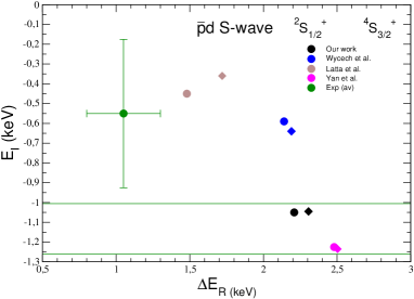
Figure 2: Comparison for the p̄d S-wave level shifts and width with previous results [30, 31, 32] are plotted.

The results displayed in Figure 2 deserve some comments. If one could explain the dispersion among the theoretical results in terms of approximate solutions, our results are exact in the numerical sense and the difference among the KW and Jülich models is not significant. Nevertheless our predictions are in strong conflict with the spin averaged experimental values, in particular for the level shifts which differ by a factor 2. These are spin average S-wave values but notice that ²S_1/2 (filled circles) and ⁴S_3/2 (filled diamonds) are almost degenerate in all the calculations. Since such a discrepancy is not observed in protonium, it would be interesting to have an experimental confirmation of the p̄d S-wave level shifts to clarify this point. The S-wave level shifts and widths probe the short range part of the interaction and is a privileged path to access the strong and annihilation N̄N forces.

Concerning the p̄d experimental results one has not been able yet to disentangle the hyperfine splitting of atomic levels. These levels are indeed strongly overlapping due to their large widths, complicating their differentiation. However, the weighted average values of level shifts and widths for S and P states have been measured at LEAR [24, 25, 26]. The comparison of our spin-averaged calculated values for L=0 and L=1 states is made in Table 4. The theoretical predictions for S-states are very stable with respect to all the considered NN and N̄N potentials. If the width falls inside the experimental error it is indeed quite worrying that the level shif represents almost double of the measured ones. The theoretical discrepancies in the 2P level shifts is much larger, and differ by one order of magnitude from the experimental values. Nevertheless, in this case, the spread between the model predicted values is also significant. One may hope that this discrepancy with phenomenology might be resolved in the near future, once more accurate N̄N data will allow to fix the N̄N interaction parameters in P-waves. Any experiment aiming to identify the bound or resonant states in N̄N P-waves would be more than welcome.

	MT13	AV18	INOY	I-N3LO	I-N3LO	Ref. [30]	Exp.
	+KW	+KW	+KW	+KW	+Jülich
L=0 $\Delta$E(eV)	2297	2194	2268	2274	2250	2170	1050$\pm$250 [24, 25, 26]
L=0 $\Gamma$ (eV)	1982	2129	1971	2095	2344	1250	1100$\pm$750 [24, 25, 26]
							2270$\pm$260 [25]
L=1 $\bigtriangleup$E (meV)	26.6	22.5	20.7	18.2	-1.1	52	243$\pm$26 [25]
L=1 $\Gamma$ (meV)	428	414	420	420	416	422	489$\pm$30 [25]

Table 4: Spin-averaged level shifts ($\Delta E_{R}$) and widths ($\Gamma$) compared to LEAR experimental results

3.3 Annihilation densities

The p̄d complex energies $E_{n}$ are obtained as eigenvalues of the FE and control the asymptotic behavior of the solution. They can alternatively be obtained in terms of the total p̄pn wavefunction in an integral form

$$\Delta E=E_{R}-i\;{\Gamma\over 2}=<\Psi_{\bar{p}d}\mid H_{0}+V\mid\Psi_{\bar{p}d}>$$

what constitutes a robust test for the calculations. In particular, taking the non Hermitian part of this expression provides an integral form for $\Gamma$, in terms of the imaginary part of the optical potential (3)

$${\Gamma}=2\int_{0}^{\infty}y^{2}dyx^{2}dx\;{\rm Im}[W(x,y)]\mid\Psi_{\bar{p}d}\mid^{2}=\int_{0}^{\infty}dr\;\gamma_{a}(r)$$ (21)

where $r$ is de distance between p̄ and deuteron center of mass ($r={\sqrt{3}\over 2}y$ with our conventions for the Jacobi coordinates (see Fig. 1). The function $\gamma_{a}(r)$, named annihilation density, can be interpreted as the probability for an p̄ to be annihilated with a proton or with a neutron at a distance r from the center of mass of the target nucleus.

One of the aims of our work was to obtain the p̄d annihilation density $\gamma^{\bar{p}d}_{a}$ and compare it with the deuteron density $\rho_{d}$. It is also interesting to compare the same quantity in absence of any matter density, that is with the p̄p (protonium) case ($\gamma^{\bar{p}p}_{a}$), considering p as point-like particles [8]. This is done in Figure 3 for p̄d S- and P-states. We have arbitrarily normalized the different quantities – $\gamma^{\bar{p}d}_{a}$, $\gamma^{\bar{p}p}_{a}$ and $\rho_{d}$ – for the sake of comparison.

For the ²S_1/2 (left panel), $\gamma^{\bar{p}d}_{a}$ (solid red line) is peaked around r=2 fm but the comparison with the ¹S₀ $\gamma^{\bar{p}p}_{a}$ (dashed blue line) tell us that this process is driven by the deuteron density (dashed black line) since a substantial part of it takes place at $r>2$. An even nicer picture is obtained for the ⁴P_5/2 state: the absorbtion density maximum is situated at $r\approx 3$ fm and scales nicely with the peripheral (r$>$3 fm) deuteron density. On the contrary, the protonium ¹P₁ annihilation is centered at around $r=0.8$ fm.

One may conclude that in the P-states antiprotons are absorbed mostly at the surface of the nucleus, thus confirming the intuitive conjecture on which the PUMA project, aiming to study peripheral neutron densities in the exotic nuclei, is based. On the contrary in S-wave antiprotons penetrate easily into the nucleus and their annihilation is less peripheral. Finally, for L$>$1 angular momentum states annihilation should be even more peripheral. Therefore the comparison of the annihilation products from different angular momentum states could provide a hint on the radial evolution of the neutron/proton ratio in the target nucleus.

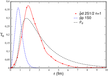
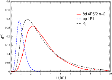
Figure 3: p̄d annihilation densities $\gamma_{a}$ for the 2S1/2 (left panel) and 4P5/2 (right panel) states calculated with the MT13+KW model. They are compared with the p̄p ¹S₀ and ¹P₁ $\gamma_{a}$’s in protonium and with corresponding deuteron matter density $\rho_{d}$.

3.4 p̄d scattering lengths and Trueman relation

By adding the corresponding inhomogeneous term in the Faddeev equations (13-17) we have calculated the p̄-d scattering ”lengths” $a_{L}$. Although these values could be approximately obtained, as in the protonium case [34], from the complex level shifts $\Delta E_{n}$ by using the Trueman relation [35], we preferred to proceed in the reverse order. That is, insert in Trueman relation the computed $a_{L}$ values and compare the $\Delta E_{n}$ thus obtained with the exact $\Delta E_{n}$ values displayed in Tables 1 and 2.

Indeed, Trueman demonstrated in [35] that the low energy parameters of two opposite-charged particles are related to the energy-shifts of their atomic states according to an expansion

$${\Delta E_{n}\over E^{c}_{n}}\approx-{4\over n}\alpha_{nL}{a_{L}\over B^{2L+1}}\left[1-\beta_{nL}{a_{L}\over B^{2L+1}}\right]+...$$ (22)

where $a_{L}$ are the Coulomb corrected scattering ”lengths”, B is the corresponding Bohr radius, and $\alpha_{nl},\beta_{nL}$ some numerical coefficients (see [34] for details). We have shown in [34] that these relations turn to be very accurate for p̄p atomic states. It is not obvious, however, how well these relations hold for a p̄ scattering on a composite nucleus, where the nuclear charge is distributed over a significant volume. Furthermore if it is not spherically symmetric, thus giving rise to long-range Coulomb multipole terms and breaking the conservation of spin quantum number. Indeed, due to the presence of quadrupole moment in deuteron, the effective p̄-d interaction has an asymptotic $1/r^{3}$ terms beyond the attractive Coulomb term.

The accuracy of expansion (22) for the p̄-d system is shown in Table 5 with two combinations of NN and N̄N models. The computed scattering ”lengths” $a_{L}$ are given in the first column, the $\Delta E$ values obtained by expansion (22) are given in columns $\Delta E_{1}$ and $\Delta E_{2}$, representing respectively corrections up to the first and the second order. Column $\Delta E$ represent the exact values obtained via direct bound state calculation and imported from Table 1.

These results demonstrate that Trueman expansion (22) works reasonably well with MT13+KW and AV18+KW interactions and for the p̄d scattering states that have spin-uncoupled asymptotic channels: $J^{\pi}$=$1/2^{-}$, $J^{\pi}$=$3/2^{-}$ and $J^{\pi}$=$5/2^{+}$ on Table 5. Likewise for p̄p case, the S-waves require second order corrections, whereas for P-wave the first order results are already accurate to four significant digits. However we have found that for the spin-coupled p̄d channels (like e.g. P_1/2 and P_3/2), the standard, Coulomb-corrected, effective range formulae fails. Indeed, if the target nucleus is non-spherically symmetric, the asymptotic p̄-A interaction acquires, beyond the Coulomb interaction, higher multipole terms, starting with the $1/r^{3}$ quadrupole ones. These terms are diagonal in total spin basis, but due the fact that strong interaction does not conserve the total spin, the p̄-A states are a mixture of different spin states. Therefore coupled p̄A channels remain asymptotically coupled by quadrupole interaction terms. In this case, a modified effective range formulae must be derived and expansion (22) reformulated accordingly. This tedious task is beyond the scope of this paper.

The validity of the Trueman relations, as an indirect way to obtain the antiproton-nucleus level shifts, is a crucial asset in view of the theoretical aspects of the PUMA project. Indeed, the computation of p̄-nucleus scattering lengths turns to be a much easier task than determining the tiny energy shifts of the atomic levels. If one could rely on this indirect approach to obtain the p̄A level shifts, this will offer the possibility to extended the rigorous theoretical calculations to more complex structures than deuteron. Using the deuteron nuclear target we have demonstrated that this is indeed the case. Nevertheless one should bare in mind that these relations should be redefined if strong magnetic interaction terms are present, as it will happen for non-spherical nuclear targets.

MT13 +KW
	$a_{0}$ (fm)	$\Delta E_{1}$ (keV)	$\Delta E_{2}$ (keV)	$\Delta E$ (keV)
${}^{2}S_{1/2}$ n=1	1.596-0.8569i	2.463-1.322i	2.259-1.014i	2.251-1.004i
${}^{4}S_{3/2}$ n=1	1.647-0.8419i	2.541-1.299i	2.316-0.987i	2.321-0.984i
	$a_{1}$ (fm3)	$\Delta E_{1}$ (meV)	$\Delta E_{2}$ (meV)	$\Delta E$ (meV)
${}^{4}P_{5/2}$ n=2	0.450-2.68i	34.8-207i	34.8-207i	26.2-215i
AV18 +KW
	$a_{0}$ (fm)	$\Delta E_{1}$ (keV)	$\Delta E_{2}$ (keV)	$\Delta E$ (keV)
${}^{2}S_{1/2}$ n=1	1.505-0.8779i	2.323-1.355i	2.155-1.057i	2.147-1.044i
${}^{4}S_{3/2}$ n=1	1.59-0.8771i	2.541-1.354i	2.257-1.039i	2.218-1.075i
	$a_{1}$ (fm3)	$\Delta E_{1}$ (meV)	$\Delta E_{2}$ (meV)	$\Delta E$ (meV)
${}^{4}P_{5/2}$ n=2	0.469-2.57i	36.4-199i	36.4-199i	39.9-204i

Table 5: Atomic level shifts, calculated from p̄d scattering lengths ($a_{0}$ and $a_{1}$) employing Trueman relations at first order ($\Delta E_{1}$) and second order ($\Delta E_{2}$) are compared with the values obtained from direct binding energy calculations ($\Delta E$).

4 Concluding remarks

We have presented In this letter the first rigorous calculation of the antiproton-deuteron states based on a coupled (p̄pn)-(n̄nn) three-body system interacting with realistic NN and N̄N optical models.

The complex energies of the low lying states as well as the corresponding scattering lengths and volumes have been obtained for several combinations of NN and N̄N models. The S-wave energy shifts of atomic p̄d energy levels are model independent but are not compatible with the measured quantities by a factor two. The corresponding widths fall inside the (large) experimental error bars. On the contrary, the P-waves are strongly model dependent and does not tolerate any approximations in the solution of the 3-body problem. Such a dependence may be due to the presence of a nearthreshold singularities in the P-waves amplitudes, making the system very sensitive to small changes in the theoretical input: they can easily transform a loosely bound P-wave 3-body bound state into a resonance with the corresponding change of sign in the p̄d level shitfs.

The p̄ annihilation densities for an S- and P-sate have been computed and found to follow closely the deuteron density up to 5-10 fm. A substantial part of the annihilation process, compared to the p̄p case, takes part in the tail part of deuteron.

We have investigated the validity of the Trueman relation, established for point like particle scattering, to the case of a composite target and found it to be accurate enough at the second order for spin-uncoupled channels. For the spin-coupled channels the Trueman relation should be generalized to account for the possible coupling in the asymptotic channel induced by $1/r^{3}$ quadrupole terms.

The actual goal of the PUMA experiment is to study the nuclear surface densities using antiproton-nucleus annihilation. It is assumed that a substantial part of the annihilation process takes place in the outer shell of the nucleus and that hey can be used to probe the peripheral matter density. This hypothesis is essentially confirmed by our results on deuteron. The presented p̄d annihilation densities shows that, although for S-wave the antiproton is able to penetrate deeply inside the deuteron, an important fraction of annihilations takes place at large distance from the center. This is even more visible for P-waves where the annihilation process is displaced toward the nuclear periphery. In any case, the annihilation density follows closely the asymptotic density profile of the deuteron. This fact provides strong support for the major hypothesis of the PUMA experiment, as most of the relevant annihilation signal is expected to happen from high angular momentum orbitals.

References

- [1] C. J. Batty, Rep. Prog. Phys. 52 (1989) 1165
- [2] M. Augsburger et al, Nucl. Phys. A658 (1999) 149
- [3] E. Klempt, F. Bradamante, A. Martin, J.M. Richard, Phys Rep 368 (2002) 119
- [4] D. Gotta, Prog. Part. Nucl. Phys. 52 (2004) 133-195
- [5] E. Klempt, Ch. Batty, J.M Richard Phys Rep 413 (2005) 197-317
- [6] J.M. Richard, Front. Phys. 8 (2020) 6
- [7] A. Obertelli et al, PUMA Letter of Intent, CERN-SPSC-2019-033 ; SPSC-P-361https://cds.cern.ch/record/2691045?ln=frhttps://home.cern/news/news/physics/cern-approves-two-new-experiments-transport-antimatter
- [8] J. Carbonell, G. Ihle, J.M. Richard, Z. Phys. A 334 (1989) 329-341
- [9] R. Lazauskas, J. Carbonell, Few-Body Sys. 31, 125(2002); Few-Body Sys. Suppl. 14 (2003) 167
- [10] R. Lazauskas, J. Carbonell, Phys. Rev. C 71, 044004 (2005)
- [11] C.B. Dover and J.M. Richard, Phys. Rev. C21 (1980) 1466.
- [12] J. Cote, M. Lacombe, B. Loiseau, B. Moussallam, R. Vinh Mau, Phys. Rev. Lett. 48, 1319 (1982)
- [13] J.M. Richard, M.E. Sainio, Phys. Lett. B 110, 349 (1982)
- [14] P.H. Timmers, W.A. van der Sanden, J.J. de Swart, Phys. Rev D 29 (1984) 1928
- [15] M. Kohno, W. Weise, Nucl. Phys. A454, 429 (1986)
- [16] B. El-Bennich, M. Lacombe, B. Loiseau and S. Wycech, Phys. Rev. C79, 054001 (2009)
- [17] Ling-Yun Dai, Johann Haidenbauer, Ulf-G. Meißner , JHEP 1707 (2017) 078
- [18] Stephen Gasiorowicz., Elementary Particle Physics. Wiley, New York, 1966
- [19] D. Baye, Phys. Rep. 565 (2015) 1.
- [20] R.A. Malfliet and J.A. Tjon, Nucl. Phys. A127 (1969) 161.G. L. Payne, J. L. Friar, and B. F. Gibson, Phys. Rev. C 26, 1385 (1982)
- [21] R. B. Wiringa, V.G.J. Stoks and R. Schiavilla, Phys. Rev. C 51 (1995) 38.
- [22] P. Doleschall, Phys. Rev. C 69 (2004) 054001.
- [23] D.R. Entem and R. Machleidt, Phys. Rev. C 68 (2003) 041001.
- [24] M. Augsburger et al., Phys. Lett. B 461 (1999) 417
- [25] D. Gotta et al., Nucl. Phys. A 660 (1999) 283.
- [26] D. Gotta, AIP Conf.Proc. 793 (2005) 169-182
- [27] J. Carbonell, O.D. Dalkarov, K.V. Protasov, I.S. Shapiro, Nucl. Phys. A535(1991)651-668
- [28] I. S. Shapiro, Phys. Rep. 35C (1978)129
- [29] C.B. Dover, J. M. Richard, Ann. Phys. 121 (1979) 70
- [30] S. Wycech, A.M. Green, J.A. Niskanen, Phys. Lett. B152 (1985) 308
- [31] G.P. Latta and P.C. Tandy, Phys. Rev. C42 (1990) R1207
- [32] Y. Yan et al., Phys. Lett. B659 (2008) 555; Erratum: Phys.Lett. B665 (2008) 425
- [33] R. Schiavila et al, Phys. Rev C58 (1998) 1263E. Epelbaum, Nuclear Physics A 747 (2005) 362?424; Eur. Phys. J. A 51 (2015) 5, 53
- [34] J.Carbonell, J.M. Richard and S.Wycech, Z.Phys. A343 (1992) 325.
- [35] T.L. Trueman, Nucl. Phys. 26, 57 (1961)