Stable determination by a single measurement, scattering bound and regularity of transmission eigenfunction

Abstract.

In this paper, we study an inverse problem of determining the cross section of an infinitely long cylindrical-like material structure from the transverse electromagnetic scattering measurement. We establish a sharp logarithmic stability result in determining a polygonal scatterer by a single far-field measurement. The argument in establishing the stability result is localised around a corner and can be as well used to produce two highly intriguing implications for invisibility and transmission resonance in the wave scattering theory. In fact, we show that if a generic medium scatterer possesses an admissible corner on its support, then there exists a positive lower bound of the $L^{2}$-norm of the associated far-field pattern. For the transmission resonance, we discover a quantitative connection between the regularity of the transmission eigenfunction at a corner and its analytic or Fourier extension.

Keywords:   Inverse medium scattering, single far-field pattern, logarithmic stability, corner singularity, invisibility, transmission resonance.

2010 Mathematics Subject Classification:  35R30, 78A46, 35Q60, 35P25,

1. Introduction

1.1. Mathematical setup and physical background

Initially focusing on the mathematics but not the physics, we introduce the scattering system for our study. Let $k\in\mathbb{R}_{+}$ be a wavenumber and $u^{i}$ be an entire solution to the Helmholtz equation,

$$\Delta u^{i}+k^{2}u^{i}=0\quad\mbox{in}\ \ \mathbb{R}^{2}.$$ (1.1)

Let $\varepsilon,\mu\in L^{\infty}(\mathbb{R}^{2})$ be real-valued functions such that $\mbox{supp}(\varepsilon-1),\mbox{supp}(\mu-1)\subset D$ and $\varepsilon,\mu\geq c_{0}\in\mathbb{R}_{+}$, where $D$ is a bounded Lipschitz domain such that $\mathbb{R}^{2}\backslash\overline{D}$ is connected. Consider the following scattering system for $u=u^{i}+u^{s}\in H_{loc}^{1}(\mathbb{R}^{2})$:

$$\begin{cases}\mbox{div}(\varepsilon^{-1}\nabla u)+k^{2}\mu u=0&\mbox{in }\mathbb{R}^{2},\vskip 6.0pt plus 2.0pt minus 2.0pt\\ r^{1/2}(\partial_{r}-\mathrm{i}k)(u-u^{i})\rightarrow 0&\mbox{while }r:=|x|\rightarrow\infty,\end{cases}$$ (1.2)

where $\mathrm{i}:=\sqrt{-1}$.

In the physical context, (1.2) describes the transverse magnetic scattering due to the impingement of an incident field $u^{i}$ on an infinitely long cylindrical material structure whose cross section is $D$; see e.g. [36] for more detailed discussion. Here, $\varepsilon$ and $\mu$ are respectively the electric permittivity and magnetic permeability, which characterize the medium parameters. The medium outside the material structure is uniformly homogeneous. $u^{s}$ signifies the perturbation of the incident field due to the presence of the inhomogeneous medium and is referred to as the scattered field. The last limit in (1.2) is called the Sommerfeld radiation condition which characterizes the outgoing nature of the scattered field. The well-posedness of the scattering system (1.2) is known (cf. [44, 51]), and moreover the following asymptotic expansion holds (cf. [18]):

$$u(x)=u^{i}(x)+\frac{e^{\mathrm{i}k|x|}}{|x|^{1/2}}u_{\infty}(\hat{x};u^{i})+\mathcal{O}(|x|^{-1})\ \ \mbox{as}\ \ |x|\rightarrow+\infty,$$ (1.3)

which holds uniformly in the angular variable $\hat{x}:=x/|x|\in\mathbb{S}^{1}$. The function $u_{\infty}:\mathbb{S}^{1}\rightarrow\mathbb{C}$ is called the far-field pattern to the scattering problem.

It is noted that the transverse electric scattering can be described similarly with the first equation in (1.2) replaced by ${\rm div\;}(\mu^{-}\nabla u)+k^{2}\varepsilon u=0$. In order to unify our discussion, we introduce the following scattering system

$$\begin{cases}\mbox{div}(\sigma\nabla u)+k^{2}qu=0&\mbox{in }\mathbb{R}^{2},\vskip 6.0pt plus 2.0pt minus 2.0pt\\ r^{1/2}(\partial_{r}-\mathrm{i}k)(u-u^{i})\rightarrow 0&\mbox{while }r\rightarrow\infty,\end{cases}$$ (1.4)

where $(\sigma,q)$ may be either $(\varepsilon^{-1},\mu)$ or $(\mu^{-1},\varepsilon)$. The inverse scattering problem that we are concerned with associated with the scattering system (1.4) in this article is to recover $D$, independent of $\sigma$ and $q$, by knowledge of $u^{\infty}$ corresponding a single incident field $u^{i}$, namely

$$u^{\infty}\ \mbox{corresponding to a fixed }u^{i}\longrightarrow D,\ \mbox{independent of }\sigma\mbox{ and }q.$$ (1.5)

1.2. Summary of main results and connection to existing studies

The inverse problem (1.5) is a fundamental one in the inverse scattering theory for electromagnetic waves, and there are rich results in the literature (cf. [18, 49, 55]). However, the determination by a single far-field measurement in the general case still remains to be an open problem; see [40] and the references cited therein for more relevant discussions. For the convenience of the readers to have a global picture of our result, we briefly summarize the major discovery in this article in what follows.

Suppose that $\sigma$ is of the form:

$$\sigma:=1+(\gamma-1)\chi_{D}$$ (1.6)

where $\gamma\neq 1$ is a positive constant and $q\in L^{\infty}$ with $\mbox{supp}(q-1)\subset D$. We write $(D;\gamma,q)$ to signify such a medium scatterer. The main stability result established in this paper for the inverse problem (1.5) can be stated as follows.

Theorem 1.1.

Let $(D;\gamma,q)$ and $(D^{\prime};\gamma^{\prime},q^{\prime})$ be two medium scatterers as described above, where $D$ and $D^{\prime}$ are assumed to be convex polygons in $\mathbb{R}^{2}$. Let $u$ and $u^{\prime}$ the corresponding solutions to the scattering system (1.4) associated with $(D;\gamma,q)$ and $(D^{\prime};\lambda^{\prime},q^{\prime})$ respectively. Suppose that the solutions $u$ and $u^{\prime}$ as well as the incident field $u^{i}$ satisfy the admissible assumptions, which will be detailed in Theorem 2.5. Denote by $u_{\infty}$ and by $u^{\prime}_{\infty}$ the far-filed patterns respectively, and suppose that

$$\|u_{\infty}-u^{\prime}_{\infty}\|_{L^{2}(\mathbb{S}^{1})}\leq\varepsilon,$$ (1.7)

where $\varepsilon\in\mathbb{R}_{+}$ and $\varepsilon\ll 1$. Then there exist constants $C,\beta>0$ which depend only on the a-priori parameters such that when $\varepsilon>0$ is sufficiently small,

$$d_{\mathcal{H}}(D,D^{\prime})\leq C(\ln|\ln\varepsilon|)^{-\beta}.$$ (1.8)

Here $d_{\mathcal{H}}$, defined later by (2.7), signifies the Hausdorff distance between two domains.

It is known that stability estimates of logarithmic type are generically optimal for inverse shape problems (cf. [42, 43, 39, 7]). Hence, it is unobjectionable to claim that our stability result in Theorem 1.1 is sharp. As mentioned earlier, the determination by a single far-field measurement is a challenging problem in the literature. Our study is closely related to two recent works [11, 7]. In [7], a similar stability estimate was established, but for the case $\sigma\equiv 1$. That is, the determination of the inhomogeneous support of the coefficient in the zeroth-order term of the elliptic PDE in (1.4). In [11], the general case with an inhomogeneous coefficient appearing in the leading-order term was considered, but only a qualitative uniqueness result was established. Hence, our result sharply quantify the uniqueness result in [11]. We would like to point out that in [7] and [11], both two and three dimensions are considered, whereas in the current article we only consider the two-dimensional case. Moreover, in [11], the coefficient $\gamma$ can be variable but fulfilling certain conditions, whereas in our study, $\gamma$ is assumed to be a constant. There are technical reasons for us doing so as discussed in what follows.

The mathematical strategy developed in this article is partly inspired from the method used in [7]. It begins with an integral identity, which can be established by applying Green’s formula on a neighborhood of the scatterer. The second step is to construct a suitable family of functions, which are referred to as the Complex-Geometrical-Optics (CGO) solutions. The third step is to estimate the two sides of the integral identity in order to give an estimation of the geometrical parameters in terms of the estimation of the solutions near the scatterer. We shall use the quantitative estimation of the unique continuation property [1] to give an estimation of solutions near the scatterer in terms of the far-field patterns. We finally shall choose delicately the right CGO solution to derive our main stability result. It is particularly noted that there is a challenging point comes from the discontinuity of the leading-order coefficient (cf. (1.6)). To overcome this difficulty, we shall make use of the corner singularity decomposition theory (see Section 2 for more details). It is noted that the corner singularity in three dimensions can be much more complicated, which include both the edge and the vertex singularities. This makes the singular behaviours of the solutions to elliptic PDEs radically more complicated. This is also the main reason that we are confined within the two dimensions in the current study. It is also the technical reason that we assume that $\gamma$ in (1.6) is constant, since otherwise the induced singularity in the solution due to the singularity of the coefficient coupled with the geometric singularity can be highly complicated. That is, as long as the singularity decomposition theory is well understood, our study can be extended to more general scenarios in high dimensions with variable coefficients. Nevertheless, as can be seen from our subsequent analysis that in principle, we only make use of the fact that $\gamma$ is a constant in a neighbourhood of any corner on $\partial D$ and it can be variable in the rest part of $D$. However, in order to ease the exposition, we assume that $\gamma$ is constant in the whole domain. Here, we would also like to mention in passing some related studies for the so-called Calderon’s inverse problem [45, 46] and inverse obstacle problems [13, 14, 28, 29, 30, 37, 38, 41, 48, 50].

In addition to its significance in the inverse scattering theory, the stability result can yield interesting implications to the invisibility which is a topic that has received considerable attentions recently. It is shown in [9] that if $\mbox{supp}(q)$ (assuming $\sigma\equiv 1$) possesses a corner, then it scatters every incident field nontrivially, namely the corresponding far-field pattern cannot identically vanish. This result is further quantified in [7] by showing the corner scatters stably in the sense that the energy of the far-field pattern possesses a positive lower bound. As an immediate consequence of Theorem 1.1, one can show that a convex polygonal material structure $(D;\sigma,q)$ scatters stably. The most interesting part is that we can show such a stable scattering result for a scatterer with a generic shape as long as it possesses a corner since our argument in establishing Theorem 1.1 can be localized around the corner. Another highly intriguing implication is about the analytic or Fourier extension of the transmission eigenfunction. We make a novel discovery on a quantitative relation between the regularity of the transmission eigenfunctions at a corner and their analytic or Fourier extensions. We shall present more details in Section 5. These intriguing topics have received considerable attentions recently in the literature, and we refer to [2, 3, 4, 5, 6, 8, 12, 15, 16, 22, 23, 24, 25, 26, 27, 47, 53, 54] as well as a survey paper [40] for more existing developments in different physical contexts.

The rest of this paper is organized as follows. In Section 2, we first discuss the corner singularity decomposition, which is a critical ingredient in our study. Then we introduce some admissibility assumptions on the geometric setup as well as the incident fields. In Section 3, we establish a quantitative estimation of the difference between two wave functions near the scatterer knowing that their far-field patterns are close enough. In Section 4, we focus our analysis on a neighborhood of a vertex on the scatterer. We establish in this region the fundamental integral identity. Then by a highly delicate analysis, we derive our stability estimate. In Section 5, we study the stable scattering due to a corner as well as the transmission resonance, which are quantitative byproducts of our stability study.

2. Geometrical setup and statement of the main results

2.1. Corner singularity decomposition

One of the key ingredients to derive the stability theorem is the local decomposition of solutions to transmission problems in a neighborhood of each polygonal vertex. This is known from the pioneering works of Kondrat’ev [34], Grisvard [32] and from Kozlov, Maz’ya, Rossemann [35] that the solution to a boundary value problem $\Delta u=f$ in a domain with a polygonal corner can be written as the sum of a regular part and a singular part. The singular part is composed of a discrete family of special functions which are explicit in terms of the underlying geometrical parameters. This result is extended to transmission problems, and we refer to Kellogg [33], Dauge and Nicaise [20, 52]. For the boundary value problem associated with the Helmholtz equation system, the same decomposition as the Laplacian case holds [17]. The transmission problems for the Helmholtz systems are also studied by Costabel [19] in a framework of the layer potential techniques. We summarize those results into the following theorem:

Theorem 2.1 (Local decomposition of solutions to transmission problems).

Let $u\in H^{1}_{loc}(\mathbb{R}^{2})$ be the solution to (1.4) with $\sigma$ satisfying (1.6), in which $D$ represents a convex polygon. We assume also that $u$ satisfies the asymptotic behavior (1.3) at infinity with a nonzero incident field $u^{i}\in H^{2}_{loc}(\mathbb{R}^{2})$. We denote by $\mathcal{S}_{D}$ the set of vertices of $D$. Here the variables $r$, $\theta$ are related to the polar coordinates in the neighborhood of each vertex. Then the following decomposition holds,

$$u=u_{reg}+\sum_{x_{i}\in\mathcal{S}_{D}}K_{i}r^{\eta_{i}}\phi_{i}(\theta)\zeta_{i}.$$ (2.1)

We have also the following properties:

1. Let $B_{R}$ be the central ball with a radius $R>0$ such that $D\Subset B_{R}$. $u_{reg}|_{D}\in H^{2}(D)$, $u_{reg}|_{B_{R}\setminus\overline{D}}\in H^{2}(B_{R}\setminus\overline{D})$, and $u_{reg}$ is continuous across $\partial D$.

2. There holds

   $$\|u_{reg}\|_{H^{2}(D)}\leq C\|u\|_{H^{1}(B_{R})},$$ (2.2)

   where the constant $C$ is independent of the shape of $D$. The same regularity estimate holds for $u_{reg}$ in $B_{R}\setminus\overline{D}$.

3. There exists explicit formulas to calculate the coefficients $K_{i}$.

4. The exponent $\eta_{i}\in(0,1)$ satisfies the following equation

   $$\left(\frac{\sin\eta_{i}(\pi-a_{i})}{\sin\eta_{i}\pi}\right)^{2}=\left(\frac{\gamma+1}{\gamma-1}\right)^{2},$$ (2.3)

   where $a_{i}$ stands for the opening angle at each vertex $x_{i}$.

5. The functions $\phi_{i}$ admit the following form: $\phi_{i}(\theta)=\cos(\eta_{i}\theta+\Phi_{i,\pm})$, where the phase shits $\Phi_{i,\pm}$ are constants determined by the transmission conditions.

6. $\zeta_{i}$ is a smooth cut-off function such that $\zeta_{i}(r)=1$ if $r\leq\varrho_{i}$ and $\zeta_{i}(r)=0$ if $r\geq 2\varrho_{i}$. The radius $\varrho_{i}$ is chosen such that the disks $(B_{2\varrho_{i}}(x_{i}))_{i\in\mathcal{S}_{D}}$ do not intersect each other.

Proof.

The solution to equation (1.4) in the ball $B_{R}$ can be rewritten as the solution to the following system,

$$\begin{cases}\mbox{div}(\sigma\nabla u)=\hat{f}&\mbox{in }B_{R},\vskip 6.0pt plus 2.0pt minus 2.0pt\\ u=\hat{g}&\mbox{on }\partial B_{R},\end{cases}$$ (2.4)

where $\hat{f}=-k^{2}qu\in L^{2}(B_{R})$, $\hat{g}=u|_{\partial B_{R}}\in H^{1/2}(B_{R})$.

Then it follows from Theorem 1.6 in [52] that the solution to the transmission problem (2.4) admits the decomposition (2.1). The equation (2.3) to determine the exponents $\eta_{i}$ can be obtained by following similar calculations as those in [21]. From the equation (4.3bis) in [52], we also have an estimation of the regular part $u_{reg}$,

$$\|u_{reg}\|_{H^{2}(D)}\leq C(\|\hat{f}\|_{L^{2}(B_{R})}+\|\hat{g}\|_{H^{1/2}(\partial B_{R})}),$$ (2.5)

with a constant $C$ independent of the shape of $D$. It follows then from the trace operator on $\partial B_{R}$ that the estimate (2.2) holds. Moreover, the coefficients $K_{i}$ can be explicitly calculated by the formula (1.24) in [52] ∎

2.2. Admissibility assumptions

Before announcing our main stability result, we introduce some admissibility conditions to clarify the framework of our study.

Definition 2.2.

Let $D$ be a convex polygon in $\mathbb{R}^{2}$, $\gamma>0$ and $q\in L^{\infty}(\mathbb{R}^{2})$. We say that $(D;\gamma,q)$ belongs to the admissible class $\mathcal{D}$ if the following conditions are fulfilled:

1. $D$ is a convex polygon and $\gamma\in\mathbb{R}_{+}$ with $\gamma\neq 1$ and $\gamma\in(\gamma_{m},\gamma_{M})$, where $\gamma_{m}$ and $\gamma_{M}$ are two positive constants;

2. $D\Subset B_{R}$, where $B_{R}$ stands for the central ball at origin with a radius $R>0$;

3. There exist $0<a_{m}<a_{M}<\pi$ such that the opening of the angle at each vertex of $D$ is in $(a_{m},a_{M})$;

4. The length of each edge of $D$ is at least $l>0$;

5. The support of $q-1$ is contained in the polygon $D$, which means $q\equiv 1$ in $\mathbb{R}^{2}\setminus\overline{D}$;

6. $\|q\|_{L^{\infty}(\mathbb{R}^{2})}\leq\mathcal{Q}$ where $\mathcal{Q}>0$ is a constant.

Remark 2.3.

In fact, the inhomogeneity on both $\sigma$ and $q$ could generate the scattering waves. It is shown in [7] that the support of $q-1$ can be stably determined from a single far-field pattern under the assumption $\sigma\equiv 1$. In principle, it is possible to stably recover both the supports of $\sigma$ and $q-1$ by using in parallel the method introduced in this paper and the one in [7]. However, if we do so, the technical details will become more complicated and distract the meaning of introducing our new method. In order to have a focusing theme of our study, we are only concerned with the recovery of the support of $\sigma$ in this paper. This is the main reason for us introducing item $(5)$ in Definition 2.2.

On the other hand, we shall impose a genetic condition on the incident field $u^{i}$ such that the singular behaviors at each corner are guaranteed.

Assumption A.

Let $u^{i}\in H^{2}_{loc}(\mathbb{R}^{2})$ be an entire solution to (1.1). We denote by $S>0$ the amplitude of the incident wave $u^{i}$, which is defined by

$$\|u^{i}\|_{H^{2}(B_{2R})}\leq S,$$ (2.6)

with $R>0$ introduced in Definition 2.2. We assume in the rest of this paper that for all $(D;\gamma,q)\in\mathcal{D}$, the corresponding solution $u$ to the scattering problem (1.4)–(1.3) admits a nondegenerate singularity coefficient $K_{i}>0$ in the decomposition (2.1) at each vertex $x_{i}$ of $D$.

Remark 2.4.

It is pointed out that (2.6) is a generic condition, which can be easily fulfilled, say e.g. by the plane wave of the form $\exp\{\mathrm{i}kx\cdot d\}$, $d\in\mathbb{S}^{1}$.

As we mentioned previously in Theorem 2.1, the coefficients $K_{i}$ in (2.1) can be determined by explicit formulas. The formulas can be found in [20, 52]. In fact, each $K_{i}$ depends linearly on the incident field $u^{i}$ for fixed polygon $D$ and vertex $x_{i}$. Assumption A is in fact a generic condition except for the case when $K_{i}=0$, which means the solution to (1.4) has $H^{2}$-regularity in a neighborhood of $x_{i}$, corresponding to a very limited class of scenarios from the practical point of view.

In what follows, for $D,D^{\prime}\in\mathcal{D}$, we define

$$d_{\mathcal{H}}(D,D^{\prime})=\max\big{(}\sup_{x\in D}\mathrm{dist}(x,D^{\prime}),\sup_{x^{\prime}\in D^{\prime}}\mathrm{dist}(x^{\prime},D)\big{)},$$ (2.7)

to be Hausdorff distance between $D$ and $D^{\prime}$. In order to simplify the expressions, we shall call the following parameters $(k,R,\gamma_{m},\gamma_{M},a_{m},a_{M},l,\mathcal{Q})$ as the a-priori parameters. With those admissible assumptions and a-priori parameters, we are in a position to complete the statement of Theorem 1.1.

Theorem 2.5.

Let $k\in\mathbb{R}_{+}$ and $u^{i}\in H^{2}_{loc}(\mathbb{R}^{2})$ be a nontrivial solution to the Helmholtz equation (1.1). Let $(D;\gamma,q)$ and $(D^{\prime};\gamma^{\prime},q^{\prime})$ belong in the admissible class $\mathcal{D}$ in Definition 2.2. We consider the solutions $u,u^{\prime}\in H^{1}_{loc}(\mathbb{R}^{2})$ to the Helmholtz equation (1.4) where the corresponding functions $\sigma,\sigma^{\prime}$ are defined by (1.6). Suppose that $u^{i}$ satisfies Assumption A. We define $\displaystyle K_{m}:=\min_{x_{i}\in\mathcal{S}_{D}\cup\mathcal{S}_{D^{\prime}}}|K_{i}|>0$ as the smallest singularity coefficient among the vertices of $D$ and $D^{\prime}$.

Assume that there holds

$$\|u_{\infty}-u^{\prime}_{\infty}\|_{L^{2}(\mathbb{S}^{1})}\leq\varepsilon.$$ (2.8)

Then there exist constants $C,\beta,\widetilde{\beta}>0$ which depend only on the a-priori parameters such that when $\varepsilon\in\mathbb{R}_{+}$ is sufficiently small, one has

$$d_{\mathcal{H}}(D,D^{\prime})\leq C\left(1+\frac{S}{K_{m}}\right)^{\widetilde{\beta}}\left(\ln\ln\frac{S}{\varepsilon}\right)^{-\beta}.$$ (2.9)

3. Propagation of smallness

The proof of Theorem 2.5 involves several technical ingredients. The objective of this section is to estimate the difference $u-u^{\prime}$ of the solutions to the scattering problems near the polygonal scatterer $D$. The first step in our method is to estimate $u-u^{\prime}$ in terms of the difference on their far-field patterns $u_{\infty}-u^{\prime}_{\infty}$ in a near-field domain. The second step is to estimate $u-u^{\prime}$ and its derivative $\nabla u-\nabla u^{\prime}$ in a neighborhood of the polygonal scatterer $D$ from the near-field estimation. Combining those results, we derive the estimations of $u-u^{\prime}$ and $\nabla u-\nabla u^{\prime}$ in terms of $u_{\infty}-u^{\prime}_{\infty}$.

Proposition 3.1.

Let $w^{s}\in H^{2}_{loc}(\mathbb{R}^{2})$ be a solution to (1.1) in $\mathbb{R}^{2}\setminus B_{R}$ and satisfy the Sommerfeld radiation condition (1.3) at infinity. We denote by $w^{s}_{\infty}$ its far-field pattern and $\varepsilon=\|w^{s}_{\infty}\|_{L^{2}(\mathbb{S}^{1})}$.

We assume the a-priori bound $\|w^{s}\|_{L^{2}(B_{2R}\setminus B_{R})}\leq\mathcal{S}$ with $\mathcal{S}\geq 0$ depending on the a-priori parameters. Let $\mathcal{A}$ be a domain such that $\mathcal{A}\subset B_{2R}\setminus\overline{B_{R}}$. Then, for any smoothness index $p\in\mathbb{N}$ there exists constants $c,C>0$ depending only on $k,p,R,\mathcal{A}$ such that

$$\|w^{s}\|_{H^{p}(\mathcal{A})}\leq C\max(\varepsilon,\mathcal{S}e^{-c\sqrt{\ln(\mathcal{S}/\varepsilon)}}).$$ (3.1)

Proof.

See Proposition 5.2 and Corollary 5.3 in [7]. ∎

We next present the propagation of smallness from a near field domain up to the boundary of the polygonal scatterer. The method we use here is mainly inspired by the one in [7], and we shall adopt similar notations therein.

Proposition 3.2.

Let $Q\Subset B_{R}\subset\mathbb{R}^{2}$ be a convex polygon, $x_{c}\in\partial Q$ be a vertex of $Q$, $P\in\mathbb{N}$, $0<\alpha<1$ and $w\in H^{1}(B_{2R}\setminus\overline{Q})$. We assume that $w$ is a solution to (1.1) in $B_{2R}\setminus\overline{Q}$ and the function $\widetilde{w_{P}}:x\mapsto|x-x_{c}|^{P}w(x)$ belongs to the class $\mathcal{C}^{\alpha}$ in $B_{2R}\setminus\overline{Q}$ with a norm at most $T\geq 1$.

We assume furthermore that $|w(x)|\leq\delta$ in $B_{7R/4}\setminus\overline{B_{5R/4}}$. If

$$\delta\leq\delta_{m}=\left[\exp\exp\left(\frac{9R|\ln c_{2}|}{(1-\alpha)\min(R_{m},2R/5)}\right)\right]^{-1},$$ (3.2)

then there exists a constant $C_{0}>0$ depending only on $k$, $\alpha$, $P$ and $R$ such that,

$$|w(x)|\leq\frac{C_{0}T}{\mathrm{dist}(x,\partial Q)^{P}}(\ln|\ln\delta|)^{-\alpha},$$ (3.3)

for $x\in B_{3R/2}\setminus\overline{Q}$. Here $R_{m}$ and $c_{2}$ are constants, which depend only on $k$ and are given respectively in Lemmas 5.4 and 5.5 in [7].

Proof.

Define

$$r=r(\delta)=\frac{9R|\ln c_{2}|}{4(1-\alpha)\ln|\ln\delta|}>0.$$

It follows from the assumption of the function $\widetilde{w_{P}}$ that $w\in L^{\infty}(B_{2R}\setminus B(Q,r))$ and $\|w\|_{L^{\infty}(B_{2R}\setminus B(Q,r))}\leq r^{-P}T$. It follows in parallel from the upper bound (3.2) of $\delta$ that $4r<R_{m}$ and that $2r<2R/5<R$. We can thus apply Proposition 5.7 in [7] where the convex polygon $Q$ is replaced by the convex set $B(Q,r)$ with the parameter $\lambda=1/4$. Then it gives

$$|w(x^{\prime})|\leq CT\left(\frac{1}{r}\right)^{P}\delta^{c_{2}^{9R/(4r)+2}},$$ (3.4)

for $x^{\prime}\in B_{2R}$ and $\mathrm{dist}(x^{\prime},\partial Q)\geq 5r$. The constant $C$ is given in Lemma 5.5 in [7].

We now assume $\mathrm{dist}(x,\partial Q)<5r$, then there exists $y\in\partial Q$ such that $|x-y|\leq 5r$. By the convexity of $Q$, there exists $x^{\prime}\in\mathbb{R}^{2}\setminus Q$ such that $\mathrm{dist}(x^{\prime},\partial Q)=|x^{\prime}-y|=5r$. The upper bound of $\delta$ implies $5r\leq R/2$, and thus $|x^{\prime}|\leq|x^{\prime}-y|+|y|\leq 5r+R<2R$. Then (3.4) holds at the point $x^{\prime}$. We have also at the same time, $|x-x^{\prime}|\leq|x-y|+|y-x^{\prime}|\leq 10r$.

By virtue of the Hölder continuity of $\widetilde{w_{P}}$ and the above observations, we can deduce as follows

$$|w(x)| \leq\frac{1}{|x-x_{c}|^{P}}\left(\|\widetilde{w_{P}}\|_{\mathcal{C}^{\alpha}(B_{2R\setminus\overline{Q}})}|x-x^{\prime}|^{\alpha}+|x^{\prime}-x_{c}|^{P}|w(x^{\prime})|\right),$$

$$\leq\frac{1}{|x-x_{c}|^{P}}\left((10r)^{\alpha}T+M_{P}(|x-x^{\prime}|^{P}+|x-x_{c}|^{P})CT\left(\frac{1}{r}\right)^{P}\delta^{c_{2}^{9R/(4r)+2}}\right),$$

$$\leq\frac{(10r)^{\alpha}T}{|x-x_{c}|^{P}}+CM_{P}T\left(\frac{10^{P}}{|x-x_{c}|^{P}}+\left(\frac{1}{r}\right)^{P}\right)\delta^{c_{2}^{9R/(4r)+2}},$$

$$\leq\frac{T}{\mathrm{dist}(x,\partial Q)^{P}}\left((10r)^{\alpha}+CM_{P}(10^{P}+5^{P})\delta^{c_{2}^{9R/(4r)+2}}\right),$$ (3.5)

where $M_{P}$ is a positive constant such that $(a+b)^{P}\leq M_{P}(a^{P}+b^{P})$ holds for all $a,b\in\mathbb{R}_{+}$.

From the definition of $r(\delta)$, we have

$$r^{\alpha} =(\frac{9R|\ln c_{2}|}{4(1-\alpha)})^{\alpha}(\ln|\ln\delta|)^{-\alpha},$$

$$\frac{9R}{4r} =-\frac{1-\alpha}{\ln c_{2}}\ln|\ln\delta|=\log_{c_{2}}(|\ln\delta|^{-(1-\alpha)}).$$ (3.6)

From the condition $|\ln\delta|>1$, we further obtain

$$\delta^{c_{2}^{9R/(4r)+2}}=e^{-|\ln\delta|c_{2}^{9R/(4r)+2}}=e^{-c_{2}^{2}|\ln\delta|^{1-(1-\alpha)}}\leq\frac{1}{c_{2}^{2}|\ln\delta|^{\alpha}}\leq\frac{1}{c_{2}^{2}}(\ln|\ln\delta|)^{-\alpha}.$$ (3.7)

Combining (3),(3),(3.7) and setting

$$C_{0}=\left(\frac{45R|\ln c_{2}|}{2(1-\alpha)}\right)^{\alpha}+\frac{CM_{P}(5^{P}+10^{P})}{c_{2}^{2}},$$ (3.8)

one can readily verify that the estimate (3.3) holds for $\mathrm{dist}(x,\partial Q)<5r$.

We proceed to treat the case $\mathrm{dist}(x,\partial Q)\geq 5r$. By following a similar argument in Proposition 5.7 in [7] with the convex polygon $Q$ replaced by the convex set $B(Q,\mathrm{dist}(x,\partial Q)-4r)$ and the parameter $\lambda=1/4$, one can derive that

$$|w(x)|\leq CT\left(\frac{1}{\mathrm{dist}(x,\partial Q)-4r}\right)^{P}\delta^{c_{2}^{9R/(4r)+2}}.$$ (3.9)

The assumption $\mathrm{dist}(x,\partial Q)\geq 5r$ implies $\left(\frac{1}{\mathrm{dist}(x,\partial Q)-4r}\right)^{P}\leq\left(\frac{5}{\mathrm{dist}(x,\partial Q)}\right)^{P}$. On the other hand, it is clear that $M_{P}\geq 1$ and $0<c_{2}<1$. Thus, the desired estimate (3.3) follows from (3.7) and (3.9) with the constant $C_{0}$ evaluated by (3.8).

The proof is complete. ∎

Proposition 3.3.

Let $u,u^{\prime}\in H^{1}_{loc}(\mathbb{R}^{2})$ be the solutions of the scattering problems (1.4) under the assumptions of Theorem 2.5. Let $Q$ be the polygonal convex hull of $D$ and $D^{\prime}$, and $x_{c}$ be a vertex of $Q$. We assume that $u-u^{\prime}$ is of class $\mathcal{C}^{\alpha_{0}}$ in $B_{2R}\setminus\overline{Q}$ and that the function $x\mapsto|x-x_{c}|\nabla(u-u^{\prime})(x)$ is of class $\mathcal{C}^{\alpha_{1}}$ in $B_{2R}\setminus\overline{Q}$ where $0<\alpha_{0},\alpha_{1}<1$. The corresponding Hölder norms are denoted respectively by $T_{0}:=\|u-u^{\prime}\|_{\mathcal{C}^{\alpha_{0}}(B_{2R}\setminus\overline{Q})}$ and $T_{1}:=\||x-x_{c}|\nabla(u-u^{\prime})\|_{\mathcal{C}^{\alpha_{1}}(B_{2R}\setminus\overline{Q})}$.

Then there exists $\varepsilon_{m}>0$ depending only on $k,\gamma,R_{m},R,\alpha_{0},\alpha_{1},\mathcal{Q},S$ and $\widetilde{C_{j}}(k,R,\alpha_{j})>0$, $j=0,1$ such that if $\|u_{\infty}-u^{\prime}_{\infty}\|_{L^{2}(\mathbb{S}^{1})}\leq\varepsilon\leq\varepsilon_{m}$, it holds that

$$|u(x)-u^{\prime}(x)| \leq\widetilde{C_{0}}T_{0}\left(\ln\ln\frac{S}{\varepsilon}\right)^{-\alpha_{0}},$$ (3.10)

$$|\nabla(u-u^{\prime})(x)| \leq\frac{\widetilde{C_{1}}T_{1}}{\mathrm{dist}(x,\partial Q)}\left(\ln\ln\frac{S}{\varepsilon}\right)^{-\alpha_{1}},$$ (3.11)

for $x\in B_{3R/2}\setminus\overline{Q}$.

Proof.

The well-posedness of the forward problem stands that for any solution $v$ to the system (1.4), it holds that

$$\|v\|_{H^{1}(B_{2R})}\leq C(R,\gamma,|D|,\|q\|_{L^{\infty}(\mathbb{R}^{2})})\|u^{i}\|_{H^{2}(B_{2R})},$$ (3.12)

for some $C(R,\gamma,|D|,\|q\|_{L^{\infty}(\mathbb{R}^{2})})>0$ independent of the geometrical shape of $D$. Thus, it follows from Definition A and (2.6) that

$$\|u-u^{\prime}\|_{H^{1}(B_{2R})}\leq\|u\|_{H^{1}(B_{2R})}+\|u^{\prime}\|_{H^{1}(B_{2R})}\leq C_{f}S,$$ (3.13)

where $C_{f}>0$ depends only on $R$, $\gamma_{M}$, $\mathcal{Q}$.

We next apply Proposition 3.1 on the region $\mathcal{A}=B_{7R/4}\setminus\overline{B_{5R/4}}$ with $w^{s}=u-u^{\prime}\in H^{2}_{loc}(\mathbb{R}^{2}\setminus B_{R})$. At the same time, we use also the Sobolev embedding $H^{1}\hookrightarrow L^{\infty}$ in $\mathbb{R}^{2}$. We then have,

$$|u-u^{\prime}|_{L^{\infty}(\mathcal{A})},|\nabla(u-u^{\prime})|_{L^{\infty}(\mathcal{A})}\leq C(R)\|u-u^{\prime}\|_{H^{2}(\mathcal{A})}\leq C\max(\varepsilon,C_{f}Se^{-c\sqrt{\ln(C_{f}S/\varepsilon)}}),$$ (3.14)

where $c,C>0$ depend only on $k,R$. We can choose now

$$\varepsilon_{m}\leq C_{f}Se^{-c^{2}},$$ (3.15)

such that (3.14) holds for the second term in the maximum function if $\varepsilon\leq\varepsilon_{m}$.

Defining

$$\delta=CC_{f}Se^{-c\sqrt{\ln(C_{f}S/\varepsilon)}},$$

we can therefore choose $\varepsilon_{m}>0$ depending only on $k,R,\gamma_{M},\alpha,\mathcal{Q},S$ such that (3.15) and (3.2) hold. Then we apply Proposition 3.2, and it follows that for $x\in B_{3R/2}\setminus\overline{Q}$,

$$|u(x)-u^{\prime}(x)|\leq\widetilde{C_{0}}T_{0}\left(\ln|\ln\delta|\right)^{-\alpha_{0}},$$

$$|\nabla(u-u^{\prime})(x)|\leq\frac{\widetilde{C_{1}}T_{1}}{\mathrm{dist}(x,\partial Q)}\left(\ln|\ln\delta|\right)^{-\alpha_{1}},$$

where the constants $\widetilde{C_{0}}$ and $\widetilde{C_{1}}$ are given by (3.8), which depend only on $k$, $\alpha_{0}$, $\alpha_{1}$, and $R$. Our choice of $\delta$ implies the following inequalities,

$$|\ln\delta| =c\sqrt{\ln\frac{C_{f}S}{\varepsilon}}-\ln(CC_{f}S)=c\sqrt{\ln C_{f}+\ln\frac{S}{\varepsilon}}-\ln(CC_{f}S)$$

$$\geq\frac{c}{2}\sqrt{\ln\frac{S}{\varepsilon}}\geq\left(\ln\frac{S}{\varepsilon}\right)^{1/4},$$

under the condition that $\varepsilon_{m}$ is small enough. Here, we can update the value of $\varepsilon_{m}$, which depends only on $k,R,\gamma_{M},\alpha,\mathcal{Q},S$. Thus, for $\alpha=\alpha_{0}$ or $\alpha_{1}$,

$$\left(\ln|\ln\delta|\right)^{-\alpha}\leq\left(\ln(\ln\frac{S}{\varepsilon})^{1/4}\right)^{-\alpha}=4^{\alpha}\left(\ln\ln\frac{S}{\varepsilon}\right)^{-\alpha}.$$

By updating the values of $\widetilde{C_{0}}$ and $\widetilde{C_{1}}$, (3.10) and (3.11) hold.

The proof is complete. ∎

4. Local analysis and proof of the stability result

In this section, we analyze locally the behavior of the solutions $u,u^{\prime}$ near a polygonal corner point in order to link the geometrical parameters and the estimations of $u-u^{\prime}$. This in turn enables to prove the main stability result.

4.1. Microlocal analysis near a vertex

Lemma 4.1.

Let $D,D^{\prime}\subset\mathbb{R}^{2}$ be two open bounded convex polygons. Let $Q$ be the convex hull of $D\cup D^{\prime}$. If $x_{c}$ is a vertex of $D$ such that $\mathrm{dist}(x_{c},D^{\prime})=\mathfrak{h}$, where $\mathfrak{h}$ gives the Hausdorff distance,

$$\mathfrak{h}=d_{\mathcal{H}}(D,D^{\prime}),$$ (4.1)

then $x_{c}$ is a vertex of $Q$. If the angle of $D$ at $x_{c}$ is $a$, then the angle of $Q$ at $x_{c}$ is at most $(a+\pi)/2<\pi$.

Proof.

See the appendix in [7]. ∎

We proceed to present our microlocal analysis around a corner. Let $D$, $D^{\prime}\in\mathcal{D}$ be two admissible polygons (cf. Definition  2.2). We assume from now on that $D\neq D^{\prime}$. Let $x_{c}\in\overline{D}$ be a vertex in Lemma 4.1. Then there exists $h\in\mathbb{R}_{+}$ such that $B(x_{c},h)\cap D^{\prime}=\emptyset$. Let $Q$ be the convex hull of $D\cup D^{\prime}$ and $\mathcal{B}$ be the open disk $B(x_{c},h)$. We denote respectively by $\widetilde{D}$ and $\widetilde{Q}$ the sectors $\mathcal{B}\cap D$ and $\mathcal{B}\cap Q$. Let $b$ signify the opening of the angle of $Q$ at $x_{c}$. Then one has $a_{m}\leq b\leq(a_{M}+\pi)/2<\pi$ by Lemma 4.1. We choose the polar coordinate system such that $x_{c}$ is the origin point and $\widetilde{Q}$ coincides with the following sector,

$$\widetilde{Q}=\{(r,\theta)|0<r<h,-b/2<\theta<b/2\}.$$

We define at the same time the unit vectors $\hat{x}$ and $\hat{y}$ to represent respectively the directions $\theta=0$ and $\theta=\pi/2$.

We next define the integral contours on which we derive the estimates; see Figure 1 for a schematic illustration. Let

$$\displaystyle\Gamma^{\pm} := \partial D\cap\mathcal{B},$$

$$\displaystyle\partial S^{i}_{D} := \partial\mathcal{B}\cap D\subset\partial S^{i}_{Q},$$

$$\displaystyle\partial S^{i}_{Q} := \{(r,\theta)|r=h,-\frac{\pi+b}{4}\leq\theta\leq\frac{\pi+b}{4}\},$$

and $\partial S^{e}$ be a circular arc passing through the following three points in the polar coordinate: $(h,\frac{\pi+b}{4})$, $(-\frac{1}{\tau},\pi)$, $(h,-\frac{\pi+b}{4})$ for a $\tau>0$. We define moreover by $\widetilde{D}^{e}$ the region surrounded by the closed contour $\overline{\Gamma^{\pm}\cup(\partial S^{i}_{Q}\setminus\partial S^{i}_{D})\cup\partial S^{e}}$ (the complementary part of $\widetilde{D}$; cf. Figure 1).

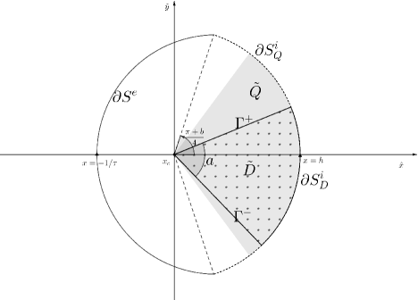
Figure 1. The sectors $\widetilde{D}$, $\widetilde{Q}$ and the integral contours.

Remark 4.2.

There are other ways to construct the integral contours here, especially for $\partial S^{e}$. The idea to construct such contours is to derive some suitable properties we can gain in the next steps. From the above construction, together with direct geometric arguments, we can obtain the following propperties:

1. for $x\in\widetilde{Q}$, $(x-x_{c})\cdot\hat{x}\geq\cos(\frac{\pi+b}{4})|x-x_{c}|$;

2. for $x\in\widetilde{D^{e}}\cup\partial S^{e}$, $(x-x_{c})\cdot\hat{x}\geq-\frac{1}{\tau}$;

3. if $\tau\geq\tau_{0}:=C_{\tau_{0}}h^{-1}=1/[2h\sin(\frac{\pi-b}{4})]$, then $\mathrm{dist}(x,\partial Q)\geq\frac{1}{2\tau}$ for $x\in\partial S^{e}$.

These properties and notations will be needed and used in our subsequent analysis.

Proposition 4.3.

Let $u,u^{\prime}$ be the solutions to (1.4) in Theorem  2.5 and $u_{0}$ be a harmonic function in $\mathcal{B}$. Then it holds that

$$(1-\gamma)\int_{\Gamma^{\pm}}u_{0}\partial_{\nu}u\,ds=\\ \int_{\partial S^{i}_{Q}\cup\partial S^{e}}(u-u^{\prime})\partial_{\nu}u_{0}-u_{0}\partial_{\nu}(u-u^{\prime})\,ds-k^{2}\int_{\widetilde{D}^{e}}(u-u^{\prime})u_{0}dx-\frac{k^{2}q}{\gamma}\int_{\widetilde{D}}u_{0}u\,dx,$$ (4.2)

where the integral over $\Gamma^{\pm}$ is taken the values of $\partial_{\nu}u$ in the interior of $\widetilde{D}$.

Proof.

This proposition follows from the transmission conditions of $u$ and $u^{\prime}$ respectively on $\partial D$ and $\partial D^{\prime}$ as well as Green’s formula along with straightforward calculations. ∎

We next introduce a special type of harmonic functions which are the so-called complex geometric optics (CGO) solutions. In this paper, we define the CGO solution as follows. Let $\tau>0$, we choose $\rho=\rho(\tau):=\tau(-\hat{x}+\mathrm{i}\hat{y})\in\mathbb{C}^{2}$. For all $x\in\mathbb{R}^{2}$,

$$u_{0}(x)=e^{\rho\cdot(x-x_{c})}.$$ (4.3)

It is easy to check that $\rho\cdot\rho=0$ and thus $u_{0}$ is harmonic in $\mathbb{R}^{2}$.

Proposition 4.4.

Let $u,u^{\prime}$ be the solutions to (1.4) and satisfy the assumptions in Theorem  2.5. Let $\tau>0$ and $u_{0}$ be a CGO solution defined by (4.3). We denote by $\Gamma^{\pm}_{\infty}$ the two rays originating from the origin and extending the segments $\Gamma^{\pm}$ to infinity (cf. Figure 1). Then it holds that

$$\int_{\Gamma^{\pm}_{\infty}}u_{0}\partial_{\nu}u_{sing}\,ds =\displaystyle\int_{\Gamma^{\pm}_{\infty}\setminus\Gamma^{\pm}}u_{0}\partial_{\nu}u_{sing}\,ds+\int_{\partial S^{i}_{D}}u_{0}\partial_{\nu}u_{reg}\,ds$$

$$-\int_{\widetilde{D}}\nabla u_{0}\nabla u_{reg}\,dx+\frac{1}{1-\gamma}\int_{\partial S^{i}_{Q}\cup\partial S^{e}}(u-u^{\prime})\partial_{\nu}u_{0}-u_{0}\partial_{\nu}(u-u^{\prime})\,ds$$

$$-\frac{k^{2}}{1-\gamma}\int_{\widetilde{D}^{e}}(u-u^{\prime})u_{0}\,dx-\frac{k^{2}q}{1-\gamma}\int_{\widetilde{D}}u_{0}u\,dx,$$ (4.4)

where $u_{sing}:=Kr^{\eta}\phi(\theta)$ and $u_{reg}$ represent the singular decomposition (2.1) of $u$ near $x_{c}$. Here, we assume the characteristics in (2.1) of $u_{sing}$ and $\zeta$ satisfy $0<\eta_{m}\leq\eta\leq\eta_{M}<1$ and $\varrho\geq h$. Then the following estimate holds,

$$C|\int_{\Gamma^{\pm}_{\infty}}u_{0}\partial_{\nu}u_{sing}ds|\leq|K|\tau^{-\eta}e^{-\alpha^{\prime}\tau h/2}+\tau^{-1}\|u_{reg}\|_{H^{2}(\widetilde{D})}+he^{-\alpha^{\prime}\tau h}\|u_{reg}\|_{H^{2}(\widetilde{D})}$$

$$+he^{-\alpha^{\prime}\tau h}(\|\partial_{\nu}(u-u^{\prime})\|_{L^{\infty}(\partial S^{i}_{Q})}+\tau\|u-u^{\prime}\|_{L^{\infty}(\partial S^{i}_{Q})})$$

$$+h(\|\partial_{\nu}(u-u^{\prime})\|_{L^{\infty}(\partial S^{e})}+\tau\|u-u^{\prime}\|_{L^{\infty}(\partial S^{e})})$$

$$+h^{2}\|u-u^{\prime}\|_{L^{\infty}(\widetilde{D}^{e})}+(\tau^{-1}+he^{-\alpha^{\prime}\tau h})\|u\|_{H^{1}(\widetilde{D})},$$ (4.5)

where $\alpha^{\prime}=\cos(\frac{\pi+b}{4})>0$, and $C$ depends only on the parameters $k,\gamma,\mathcal{Q},\eta_{m},\eta_{M},a_{m},a_{M}$.

Proof.

Using the decomposition (2.1) and the integral identity (4.2), one has

$$\int_{\Gamma^{\pm}_{\infty}}u_{0}\partial_{\nu}u_{sing}\,ds =\displaystyle\int_{\Gamma^{\pm}_{\infty}\setminus\Gamma^{\pm}}u_{0}\partial_{\nu}u_{sing}\,ds-\int_{\Gamma^{\pm}}u_{0}\partial_{\nu}u_{reg}\,ds$$

$$+\frac{1}{1-\gamma}\int_{\partial S^{i}_{Q}\cup\partial S^{e}}(u-u^{\prime})\partial_{\nu}u_{0}-u_{0}\partial_{\nu}(u-u^{\prime})\,ds$$

$$-\frac{k^{2}}{1-\gamma}\int_{\widetilde{D}^{e}}(u-u^{\prime})u_{0}\,dx-\frac{k^{2}q}{\gamma(1-\gamma)}\int_{\widetilde{D}}u_{0}u\,dx.$$ (4.6)

From Theorem 2.1, the singular function $u_{sing}$ is harmonic in $\widetilde{D}$. By further using (1.4), it holds in $\widetilde{D}$ that

$$\Delta u_{reg}+\frac{k^{2}q}{\gamma}u=0.$$ (4.7)

It follows from Green’s formula,

$$\int_{\Gamma^{\pm}}u_{0}\partial_{\nu}u_{reg}ds=-\int_{\partial S^{i}_{D}}u_{0}\partial_{\nu}u_{reg}ds+\int_{\widetilde{D}}\nabla u_{0}\nabla u_{reg}dx-\frac{k^{2}q}{\gamma}\int_{\widetilde{D}}u_{0}udx.$$ (4.8)

Inserting (4.8) into (4.1), we obtain (4.4).

We derive next the estimates of each term in the right-hand-side of (4.4). We define the integrals $I_{1},\cdots,I_{9}$ as follows,

$$I_{1} =\int_{\Gamma^{\pm}_{\infty}\setminus\Gamma^{\pm}}u_{0}\partial_{\nu}u_{sing}ds, I_{2} =\int_{\partial S^{i}_{D}}u_{0}\partial_{\nu}u_{reg}ds,$$

$$I_{3} =\int_{\widetilde{D}}\nabla u_{0}\nabla u_{reg}dx, I_{4} =\int_{\partial S^{i}_{Q}}(u-u^{\prime})\partial_{\nu}u_{0}ds,$$

$$I_{5} =\int_{\partial S^{i}_{Q}}u_{0}\partial_{\nu}(u-u^{\prime})ds, I_{6} =\int_{\partial S^{e}}(u-u^{\prime})\partial_{\nu}u_{0}ds,$$

$$I_{7} =\int_{\partial S^{e}}u_{0}\partial_{\nu}(u-u^{\prime})ds, I_{8} =\int_{\widetilde{D}^{e}}(u-u^{\prime})u_{0}dx,$$

$$I_{9} =\int_{\widetilde{D}}u_{0}udx.$$ (4.9)

From the construction of the CGO solution $u_{0}$ and Remark 4.2, we have the following properties, for $x\in\widetilde{D}\cup\partial S^{i}_{Q}\subset\widetilde{Q}$,

$$|u_{0}(x)|\leq e^{\Re(\rho)\cdot(x-x_{c})}\leq e^{-\alpha^{\prime}\tau r},$$ (4.10)

and for $x\in\widetilde{D}^{e}\cup\partial S^{e}$,

$$|u_{0}(x)|\leq e^{\Re(\rho)\cdot(x-x_{c})}\leq e^{\tau\cdot\frac{1}{\tau}}=e.$$ (4.11)

Using (4.10), (4.11) and the Sobolev embedding $H^{1}\hookrightarrow L^{\infty}$ in $\mathbb{R}^{2}$, it is shown in the proof of Proposition 4.3 in [45],

$$|I_{1}| \leq C_{1}|K|\tau^{-\eta}e^{-\alpha^{\prime}\tau h/2}, |I_{2}| \leq C_{2}he^{-\alpha^{\prime}\tau h}\|u_{reg}\|_{H^{2}(\widetilde{D})},$$

$$|I_{3}| \leq C_{3}(he^{-\alpha^{\prime}\tau h}+\frac{1}{\tau})\|u_{reg}\|_{H^{2}(\widetilde{D})}, |I_{4}| \leq C_{4}\tau he^{-\alpha^{\prime}\tau h}\|u-u^{\prime}\|_{L^{\infty}(\partial S^{i}_{Q})},$$

$$|I_{5}| \leq C_{5}he^{-\alpha^{\prime}\tau h}\|\partial_{\nu}(u-u^{\prime})\|_{L^{\infty}(\partial S^{i}_{Q})}, |I_{6}| \leq C_{6}\tau h\|u-u^{\prime}\|_{L^{\infty}(\partial S^{e})},$$

$$|I_{7}| \leq C_{7}h\|\partial_{\nu}(u-u^{\prime})\|_{L^{\infty}(\partial S^{e})},$$ (4.12)

where the constants $C_{1},\cdots,C_{7}$ depend only on the a-priori parameters.

The least two integrals $I_{8},I_{9}$ can be estimated by following the same technique above and we have

$$|I_{8}|\leq C_{8}h^{2}\|u-u^{\prime}\|_{L^{\infty}(\widetilde{D}^{e})}, |I_{9}|\leq C_{9}(he^{-\alpha^{\prime}\tau h}+\frac{1}{\tau})\|u\|_{H^{1}(\widetilde{D})},$$ (4.13)

where the constants $C_{8},C_{9}$ depend only on the a-priori parameters.

Regrouping the estimates in (4.1), (4.13), one can readily show that the inequality (4.4) holds.

The proof is complete. ∎

Proposition 4.5.

Under the same assumptions in Proposition 4.4, it holds that

$$\left|\int_{\Gamma^{\pm}_{\infty}}u_{0}\partial_{\nu}u_{sing}d\sigma\right|=|K|\Gamma(\eta)\left|\phi^{\prime}(\theta^{+})e^{\mathrm{i}a\eta}-\phi^{\prime}(\theta^{-})\right|\tau^{-\eta}\geq|K|\Gamma(\eta)\sin(a\eta)\tau^{-\eta},$$ (4.14)

where $\theta^{\pm}$ signify the arguments of the vectors along $\Gamma^{\pm}$.

Proof.

See Proposition 4.4 in [45]. ∎

4.2. Proof of Theorem 2.5

Proof.

We begin the proof by recalling some relevant results in Theorem 2.1. For any vertex $x_{0}$ of the polygon $D$ or $D^{\prime}$, the corresponding solutions $u$ or $u^{\prime}$ in a neighborhood of $x_{0}$ can be decomposed into the following form,

$$u(x)=u_{sing}(x)\zeta(r)+u_{reg}(x)=Kr^{\eta}\phi(\theta)\zeta(r)+u_{reg}(x),$$ (4.15)

where $(r,\theta)$ represent the local polar coordinate centered at $x_{0}$. As the polygons $D$ and $D^{\prime}$ satisfy the admissibility Definition 2.2, we can thus set $\varrho=l/5$ in the following proof such that the cut-off function $\zeta$ at every vertex satisfies the point (6) in Theorem 2.1. Moreover, the singularity exponents $\eta$ are explicitly determined by (2.3). Hence there exist $0<\eta_{m}<\eta_{M}<1$, which depend only on $\gamma,a_{m},a_{M}$ such that $\eta_{m}\leq\eta\leq\eta_{M}$.

Let $x_{c}$ be a vertex of $\partial D$ such that $\mathfrak{h}=\mathrm{dist}(x,D^{\prime})$. We define the integral contours in Subsection 4.1 with a radius $h=\min(\mathfrak{h}/2,l/5)$ and we reserve all the notations in Subsection 4.1. The fact $h\leq l/5\leq\varrho$ implies that the corner singularity decomposition (4.15) holds for the solution $u$ near $x_{c}$ and $\zeta\equiv 1$ in $\mathcal{B}$. Thus Proposition 4.4 and Proposition 4.5 hold as well.

Next we estimate the following norms appearing in the inequality (4.4): $\|u_{reg}\|_{H^{2}(\widetilde{D})}$, $\|u\|_{H^{1}(\widetilde{D})}$, $\|u-u^{\prime}\|_{L^{\infty}(\partial S^{i}_{Q})}$, $\|\partial_{\nu}(u-u^{\prime})\|_{L^{\infty}(\partial S^{i}_{Q})}$, $\|u-u^{\prime}\|_{L^{\infty}(\partial S^{e})}$, $\|\partial_{\nu}(u-u^{\prime})\|_{L^{\infty}(\partial S^{e})}$ and $\|u-u^{\prime}\|_{L^{\infty}(\widetilde{D^{e}})}$.

The estimates of $\|u_{reg}\|_{H^{2}(\widetilde{D})}$ and $\|u\|_{H^{1}(\widetilde{D})}$ can be obtained by a direct application of Theorem 2.1 and the well-posedness of the forward problem,

$$\|u_{reg}\|_{H^{2}(\widetilde{D})},\|u\|_{H^{1}(\widetilde{D})}\leq C\|u\|_{H^{1}(B_{R})}\leq CC_{f}S:=C_{\widetilde{D}},$$ (4.16)

where the constant $C_{\widetilde{D}}$ depends only on the a-priori parameters.

It also follows directly from the Sobolev embedding $H^{1}\hookrightarrow L^{\infty}$ in $\mathbb{R}^{2}$ and (3.12)-(3.13) that

$$\|u-u^{\prime}\|_{L^{\infty}(\partial S^{i}_{Q})}\leq C(R)\|u-u^{\prime}\|_{H^{1}(B_{R})}\leq C(R)C_{f}S:=C_{\partial S^{i},0},$$ (4.17)

where the constant $C_{\partial S^{i},0}$ depends only on the a-priori parameters.

We now estimate $\|\nabla(u-u^{\prime})\|_{L^{\infty}(\partial S^{i}_{Q})}$. It follows from Theorem 2.1 that for all $x\in\partial S^{i}_{Q}$,

$$|\nabla u(x)|\leq|K|\eta|x-x_{c}|^{\eta-1}+|\nabla u_{reg}(x)|,$$ (4.18)

as well as

$$|\nabla u^{\prime}(x)|\leq|K^{\prime}|\eta^{\prime}|x-x^{\prime}_{c}|^{\eta^{\prime}-1}\zeta^{\prime}(x)+|K^{\prime}||x-x^{\prime}_{c}|^{\eta^{\prime}}|\nabla\zeta^{\prime}(x)|+|\nabla u^{\prime}_{reg}(x)|,$$ (4.19)

where $x^{\prime}_{c}$ signifies the nearest vertex to $x_{c}$ on $\partial D^{\prime}$ and $K^{\prime},\eta^{\prime},\zeta^{\prime},u^{\prime}_{reg}$ are the corresponding elements of $u^{\prime}$ in the corner singularity decomposition (4.15). We next apply the Sobolev embedding $H^{1}\hookrightarrow L^{\infty}$ in $\mathbb{R}^{2}$ and follow analogously as (4.16), (4.18) to derive that

$$|\nabla u(x)| \leq|K|h^{\eta-1}+C(R)\|\nabla u_{reg}\|_{H^{1}(\widetilde{D^{e}})}\leq|K|h^{\eta-1}+C(R)\|u_{reg}\|_{H^{2}(\widetilde{D^{e}})},$$

$$\leq|K|h^{\eta-1}+CC(R)\|u\|_{H^{1}(B_{R})}\leq|K|h^{\eta-1}+CC(R)C_{f}S.$$

The definition of $h$ implies $h\leq\mathfrak{h}/2$, in other words, the distance for any points on $D^{\prime}$ to the ball $\mathcal{B}$ is at least $h$, and therefore $|x-x^{\prime}_{c}|\geq h$. By virtue of the cut-off function $\zeta^{\prime}$, we only need to consider the case $\varrho\leq|x-x^{\prime}_{c}|\leq 2\varrho=\frac{2l}{5}$, which in turn means that we only need to estimate the second term in the right hand side of (4.19). It is remarked that the cut-off function $\zeta^{\prime}$ depends only on $l$. Then by applying the same Sobolev embedding, we have

$$|\nabla u^{\prime}(x)| \leq|K^{\prime}|h^{\eta^{\prime}-1}+|K^{\prime}|\frac{2l}{5}\|\nabla\zeta^{\prime}\|_{L^{\infty}(\mathbb{R}^{2})}+C(R)\|u^{\prime}_{reg}\|_{H^{2}(\widetilde{D^{e}})},$$

$$\leq|K^{\prime}|h^{\eta^{\prime}-1}+|K^{\prime}|C(l)+CC(R)C_{f}S.$$

Summing up the above estimates, we can deduce the following estimate:

$$\|\nabla(u-u^{\prime})\|_{L^{\infty}(\partial S^{i}_{Q})}\leq|K|h^{\eta-1}+|K^{\prime}|h^{\eta^{\prime}-1}+|K^{\prime}|C(l)+2CC(R)C_{f}S,$$ (4.20)

Furthermore, the singularity coefficient $K^{\prime}$ can be estimated using the singular decomposition (4.15). By a direct integration of the singular function over $B_{R}$, there exists a constant $C(l,\eta_{m},\eta_{M})>0$ such that,

$$C(l,\eta_{m},\eta_{M})|K^{\prime}|\leq\|u^{\prime}_{sing}\zeta^{\prime}\|_{L^{2}(B_{R})}\leq\|u^{\prime}\|_{H^{1}(B_{R})}\leq C_{f}S.$$

Then it follows that $|K^{\prime}|\leq C_{K}S$ and hence (4.20) becomes,

$$\|\nabla(u-u^{\prime})\|_{L^{\infty}(\partial S^{i}_{Q})}\leq|K|h^{\eta-1}+C_{K}Sh^{\eta^{\prime}-1}+C_{\partial S^{i},1}S,$$ (4.21)

where the constants $C_{K},C_{\partial S^{i},1}$ depend only on the a-priori parameters.

By Theorem 2.1 we see that $u$ and $u^{\prime}$ are at least of class $\mathcal{C}^{\eta_{m}}$ in the neighborhood of $x_{c}$. The estimations of the $\mathcal{C}^{\eta_{m}}$ norms of $u$ and $u^{\prime}$ can be deduced from the decomposition formulas and the Sobolev embedding $H^{2}(\widetilde{D^{e}})\hookrightarrow\mathcal{C^{\alpha}}(\widetilde{D^{e}})$ for all $0<\alpha<1$ (see Corollary 7.11 in [31]). Using the same arguments as the estimations above, we have then,

$$\|u-u^{\prime}\|_{\mathcal{C}^{\eta_{m}}(\widetilde{D^{e}})}\leq|K|+C_{T}S,$$ (4.22)

where $C_{T}$ depends only on the a-priori data. Nevertheless, we can apply again Theorem 2.1 and the higher regularity result in [52] to derive that the functions $x\mapsto|x-x_{c}|\nabla u(x)$ and $x\mapsto|x-x_{c}|\nabla u^{\prime}(x)$ are in fact at least of class $\mathcal{C}^{\eta_{m}}$ and their $\mathcal{C}^{\eta_{m}}$ norms are also bounded by the right-hand side of (4.22). We apply now Proposition 3.3 with $\alpha_{0}=\alpha_{1}=\eta_{m}$. Then there exists $\varepsilon_{m}>0$ depending only on the a-priori parameters such that if $\varepsilon<\varepsilon_{m}$, for all $x\in\widetilde{D}^{e}\cup\partial S^{e}$,

$$|u-u^{\prime}|(x)\leq\widetilde{C_{0}}(|K|+C_{T}S)\left(\ln\ln\frac{S}{\varepsilon}\right)^{-\eta_{m}}.$$ (4.23)

In what follows, we denote by $\delta(\varepsilon)$ the quantity $(\ln\ln\frac{S}{\varepsilon})^{-\eta_{m}}$. It also follows from Proposition 3.3 and Remark 4.2 that for all $x\in\partial S^{e}$, $\frac{1}{2\tau}\leq\mathrm{dist}(x,\partial Q)$ and thus

$$|\nabla(u-u^{\prime})|(x)\leq 2\widetilde{C_{1}}(|K|+C_{T}S)\tau\delta(\varepsilon).$$ (4.24)

Next we apply Propositions 4.4 and 4.5 with the estimates (4.16), (4.17), (4.21), (4.23) and (4.24). We absorb into the left hand side all the constants depending only on the a-priori parameters. There exists a constant $C$ depending only on the a-priori parameters such that

$$C|K|\tau^{-\eta}\leq |K|\tau^{-\eta}e^{-\alpha^{\prime}\tau h/2}+S\tau^{-1}+She^{-\alpha^{\prime}\tau h}+(|K|h^{\eta-1}+Sh^{\eta^{\prime}-1}+S+S\tau)he^{-\alpha^{\prime}\tau h}$$

$$+(|K|+S)h\tau\delta(\varepsilon)+(|K|+S)h^{2}\delta(\varepsilon).$$

Using the facts that $h\leq 1$ and $\tau\geq 1$ and the inequalities $e^{-x}\leq x^{-1}$, $e^{-x}\leq x^{-2}$ for all $x>0$, we multiply on the two sides the factor $\frac{\tau^{\eta}}{|K|}$ which yields that

$$C \leq e^{-\alpha^{\prime}\tau h/2}+\frac{S}{|K|}\tau^{\eta-1}+\frac{S}{|K|}h\tau^{\eta}e^{-\alpha^{\prime}\tau h}+(h^{\eta}+\frac{S}{|K|}h^{\eta^{\prime}}+\frac{S}{|K|}h+\frac{S}{|K|}h\tau)\tau^{\eta}e^{-\alpha^{\prime}\tau h}$$

$$+(1+\frac{S}{|K|})h\tau^{\eta+1}\delta(\varepsilon)+(1+\frac{S}{|K|})h^{2}\tau^{\eta}\delta(\varepsilon),$$

$$\leq h^{-1}\tau^{-1}+\frac{S}{|K|}\tau^{\eta-1}+\frac{S}{|K|}h^{\eta-1}\tau^{\eta-1}+\frac{S}{|K|}h^{\eta^{\prime}-1}\tau^{\eta-1}+\frac{S}{|K|}\tau^{\eta-1}+\frac{S}{|K|}h^{-1}\tau^{\eta-1}$$

$$+(1+\frac{S}{|K|})h\tau^{\eta+1}\delta(\varepsilon),$$

$$\leq(1+\frac{S}{|K|})(h^{-1}\tau^{\eta-1}+h\tau^{\eta+1}\delta(\varepsilon)).$$ (4.25)

We next determine a minimum modulo constants of the right hand side of the inequality in (4.2). Set $\tau=\tau_{e}$ with

$$\tau_{e}=h^{-1}\delta(\varepsilon)^{-1/2}.$$ (4.26)

It is straightforward to verify that for $\varepsilon$ smaller than a certain constant one has that if

$$\delta(\varepsilon)^{-1/2}\geq C_{\tau_{0}},$$ (4.27)

where $C_{\tau_{0}}$ is defined in Remark 4.2, then

$$\tau_{e}\geq\tau_{0},$$

which justifies that we can take $\tau=\tau_{e}$ in (4.2).

Solving for $h$, it gives

$$h\leq C(1+\frac{S}{|K|})^{\frac{1}{\eta}}\left(\ln\ln\frac{S}{\varepsilon}\right)^{\frac{\eta_{m}(\eta-1)}{2\eta}},$$ (4.28)

and thus,

$$\min(\mathfrak{h}/2,l/5)\leq C(1+\frac{S}{K_{m}})^{\frac{1}{\eta_{m}}}\left(\ln\ln\frac{S}{\varepsilon}\right)^{\frac{\eta_{m}(\eta_{M}-1)}{2\eta_{M}}}.$$ (4.29)

Hence, if $\varepsilon$ is small enough such that $\varepsilon<\varepsilon_{m}$ in Proposition 3.3, that (4.27) holds and that the right hand side of (4.29) is smaller than $l/5$, we have

$$\mathfrak{h}\leq C(1+\frac{S}{K_{m}})^{\frac{1}{\eta_{m}}}\left(\ln\ln\frac{S}{\varepsilon}\right)^{\frac{\eta_{m}(\eta_{M}-1)}{2\eta_{M}}}.$$

Therefore, the claim of this theorem readily follows.

The proof is complete. ∎

5. Implications to invisibility and transmission eigenvalue problem

In this section, we present two interesting implications to the wave scattering theory which are byproducts of our stability study. Let us consider the scattering problem (1.4) and (1.3). It is said that invisibility occurs if

$$u_{\infty}\equiv 0.$$ (5.1)

The first byproduct we shall establish is to show that if a general scattering medium possesses a corner on its support, then the $L^{2}$-energy of the corresponding far-field pattern possesses a positive lower bound. That is, a corner scatters stably and invisibility cannot be achieved. In fact, we have

Theorem 5.1.

Let $D$ be a Lipschitz domain in $\mathbb{R}^{2}$, not necessarily a convex polygon. We assume that $\partial D$ admits a convex polygonal point, i.e. there exists $x_{c}\in\partial D$ such that $D\cap B_{l}(x_{c})$ is a plan sector for $l>0$. We denote by $0<a<\pi$ the opening of the corner $x_{c}$. Let $\gamma>0$, $\gamma\neq 1$ and $q\in L^{\infty}(\mathbb{R}^{2})$. We consider the scattering problem (1.4) where $\sigma$ is defined by (1.6) and the incident field $u^{i}\in H^{2}_{loc}(\mathbb{R}^{2})$ is a nontrivial entire solution to (1.1) in $\mathbb{R}^{2}$. We suppose the following conditions are fulfilled:

1. $D\Subset B_{R}$ for some $R>l$;

2. $0<a_{m}\leq a\leq a_{M}<\pi$;

3. $0<\gamma_{m}\leq\gamma\leq\gamma_{M}$;

4. $\mathrm{supp}(q-1)\Subset B_{R}$;

5. $\mathrm{supp}(q-1)\cap B_{l}(x_{c})\subset D\cap B_{l}(x_{c})$;

6. $\|q\|_{L^{\infty}(\mathbb{R}^{2})}\leq\mathcal{Q}$;

7. $\|u^{i}\|_{H^{2}(B_{2R})}\leq S$ for some $S>0$;

8. The solution $u$ to (1.4) admits a non-degenerate corner singularity near $x_{c}$, i.e. the singularity coefficient $K\neq 0$ in Theorem 2.1. And the singularity exponent is denoted by $0<\eta<1$.

Then there exists a constant $C$ depending only on the a-priori data $k$, $R$, $\gamma_{m}$, $\gamma_{M}$, $a_{m}$, $a_{M}$, $l$ and $\mathcal{Q}$ such that one has

$$\|u_{\infty}\|_{L^{2}(\mathbb{S}^{1})}\geq\frac{S}{\exp\exp\left(C(1+\frac{S}{|K|})^{\frac{2}{\eta(1-\eta)}}\right)}.$$ (5.2)

Proof.

The proof follows from similar arguments in the proof of Theorem 2.5 with necessary modifications. We take $D^{\prime}=\emptyset$, $q^{\prime}\equiv 1$ in $\mathbb{R}^{2}$, and therefore, $\varepsilon=\|u_{\infty}\|_{L^{2}(\mathbb{S}^{2})}$. In the current scenario, we only need to consider the effect caused by the vertex $x_{c}$, and the corresponding reasoning in the previous sections could be therefore considerably reduced. We set $h=l/5$ and $\delta(\varepsilon)=(\ln\ln\frac{S}{\varepsilon})^{-\eta}$. The inequality (4.2) still holds, and the minimum modulo constants of its right hand side occurs at $\tau_{e}$ given by (4.26). We define the constant $\varepsilon^{\prime}_{m}$ by (4.27), namely

$$\delta(\varepsilon^{\prime}_{m})^{-1/2}=C_{\tau_{0}}.$$ (5.3)

Then we set the constant $\varepsilon_{min}:=\min(\varepsilon_{m},\varepsilon^{\prime}_{m})$, where $\varepsilon_{m}$ is given in Proposition 3.3. Furthermore, it follows from (5.3) and (3.15) that $\varepsilon_{min}$ can be expressed into the following way,

$$\varepsilon_{min}=\frac{S}{\exp\exp C_{min}},$$ (5.4)

where $C_{min}$ depends only on a-priori data.

In the case $\varepsilon\leq\varepsilon_{min}$, we can take $\tau=\tau_{e}$ in (4.2). After solving for $h$, we can obtain a similar result as (4.28),

$$h\leq C(1+\frac{S}{|K|})^{\frac{1}{\eta}}(\ln\ln\frac{S}{\varepsilon})^{\frac{\eta-1}{2}},$$ (5.5)

where the constant $C$ depends only on the a-priori data.

Thus, one has

$$\|u_{\infty}\|_{L^{2}(\mathbb{S}^{1})}=\varepsilon\geq\frac{S}{\exp\exp\left(C(1+\frac{S}{|K|})^{\frac{2}{\eta(1-\eta)}}\right)}.$$ (5.6)

Combining with (5.4) and updating the constant $C$ in (5.6), the inequality (5.2) holds readily.

The proof is complete. ∎

Next, we consider the implication to the transmission eigenvalue problem. For the scattering problem (1.4), if invisibility occurs, namely (5.1) holds, one can directly verify by setting $v=u^{i}|_{D}$ that

$$\begin{cases}\mbox{div}(\sigma\nabla u)+k^{2}qu=0&\text{in }D,\vskip 6.0pt plus 2.0pt minus 2.0pt\\ \Delta v+k^{2}v=0&\text{in }D,\vskip 6.0pt plus 2.0pt minus 2.0pt\\ u=v,\quad\sigma\partial_{\nu}u=\partial_{\nu}v&\text{on }\partial D.\end{cases}$$ (5.7)

On the other hand, if there exists nontrivial solutions $u\in H^{1}(D)$ and $v\in H^{1}(D)$ to (5.7), then $k\in\mathbb{R}_{+}$ is called a transmission eigenvalue and $u,v$ are the associated transmission eigenfunctions (cf. [10]). Let $v$ be transmission eigenfunction associated with $k\in\mathbb{R}_{+}$. Then the following so-called Herglotz approximation holds, which represents a certain Fourier extension property (cf. [22, 25]). For any $\varepsilon\ll 1$, there exists $g_{\varepsilon}\in L^{2}(\mathbb{S}^{1})$ such that (cf. [56])

$$\|v_{g_{\varepsilon}}-v\|_{H^{1}(D)}\leq\varepsilon,\ \ v_{g_{\varepsilon}}(x):=\int_{\mathbb{S}^{1}}e^{\mathrm{i}kx\cdot d}g_{\varepsilon}(d)\,ds(d),$$ (5.8)

where $v_{g_{\varepsilon}}$ is referred to as a Herglotz wave function associated with the kernel density $g_{\varepsilon}$ and is an entire solution to the Helmholtz equation (1.1).

Theorem 5.2.

Let $(D,\gamma,q)$ be a convex polygonal scatter satisfying the assumptions in Theorem 2.5. We consider the transmission eigenvalue problem (5.7) with nontrivial eigenfunctions $u,v\in H^{1}(D)$ with $\|v\|_{H^{1}(D)}=1$. Then it holds that:

1. If $v$ can be extended outside $D$ to be an entire solution to (1.1), then $u\in H^{2}(D)$.

2. Let $(v_{g_{\varepsilon}})_{\varepsilon>0}$ be a family of Herglotz wave functions that are given in (5.8) and approximate the transmission eigenfunction $v$. There exist positive constants $A$ and $b$ which are independent of $g_{\varepsilon}$ such that for any given function $\psi:\mathbb{R}_{+}\rightarrow\mathbb{R}_{+}$ satisfying $\psi(\varepsilon)\rightarrow 0$ as $\varepsilon\rightarrow 0$, if $\|g_{\varepsilon}\|_{L^{2}(\mathbb{S}^{1})}\leq\psi(\varepsilon)\left(\ln\ln\frac{A}{\varepsilon}\right)^{b}$, then it holds that

   $$\lim_{x\neq x^{\prime}\in D,x,x^{\prime}\rightarrow x_{c}}\frac{|u(x)-u(x^{\prime})|}{|x-x^{\prime}|^{\eta}}=0$$ (5.9)

   at each vertex $x_{c}$ of $D$, where $\eta$ is given by (2.3).

Remark 5.3.

The Herglotz approximation property (5.8) can be regarded as a certain Fourier extension of the transmission eigenfunction $v$; see [22, 25] for more related discussion. On the other hand, if $v$ can be extended to an entire solution to (1.1), it is clear that $v$ is analytic in $\mathbb{R}^{2}$. Hence, intriguingly, Theorem 5.2 connects the local regularity of the transmission eigenfunction $u$ around a corner to the analytic or Fourier extension property of the transmission eigenfunction $v$.

Note that by the standard Sobolev embedding, $u\in H^{2}(D)$ implies that $u$ is Hölder continuous up to the boundary. Hence, the first result in the theorem indicates that if $u$ is not Hölder continuous up to a corner vertex, then $v$ cannot be analytically extended across the corner. Moreover, it further indicates that if $v$ is approximated by the Herglotz sequence $v_{g_{\varepsilon}}$, then $\|g_{\varepsilon}\|_{L^{2}(\mathbb{S}^{1})}$ must be unbounded, since otherwise $v_{g_{\varepsilon}}$ converges, by passing to a subsequence if necessary, to an entire solution to (1.1), say $v_{0}$, which is an analytic extension of $v$ into $\mathbb{R}^{2}$; see also [4, 11] for more relevant discussion about this point.

The second result in Theorem 5.2 quantitatively reinforces the above assertion about the unboundedness of the Herglotz kernels $\|g_{\varepsilon}\|_{L^{2}(\mathbb{S}^{1})}$ if the transmission eigenfunction $u$ is not Hölder continuous up to any corner vertex of the domain $D$. To illustrate this point, let us take $\psi(\varepsilon)=\left(\ln\ln\frac{A}{\varepsilon}\right)^{-b/2}$ in item (2) in the theorem. Then if $u$ is not $C^{\eta}$ up to a corner vertex, then one clearly has $\|g_{\varepsilon}\|_{L^{2}(\mathbb{S}^{1})}\geq\psi(\varepsilon)\left(\ln\ln\frac{A}{\varepsilon}\right)^{b/2}\rightarrow+\infty$ as $\varepsilon\rightarrow+0$.

It is also interesting to point out that Theorem 5.2 corroborates the studies in [22, 25], which make use of a similar Herglotz approximation property as a regularity criterion in a certain different setup from the current article.

Finally, we would like to point out that Theorem 5.2 still holds true for the case that $D$ is a generic domain but possess an admissible corner. In fact, as point out earlier, our argument can be localised around the corner and is irrelevant to the rest part of $\partial D$. Nevertheless, in order to ease the exposition, we only consider the case that $D$ is a convex polygon.

Proof of Theorem 5.2.

We assume that $v$ can be extended to be an entire solution to the Helmholtz equation (1.1), which is still denoted by $v$. It follows directly from the classic elliptic regularity that $v$ is real analytic on all compact domains in $\mathbb{R}^{2}$.

Consider the scattering problem (1.4) with $u^{i}=v$. We denote also by $u$ the extension by $v$ of $u$, the transmission conditions (5.7) on $\partial D$ implies that $u$ satisfies (1.4) in $\mathbb{R}^{2}$ and

$$u_{\infty}(\hat{x};v)\equiv 0.$$ (5.10)

We then apply Theorem 5.1 at each vertex of the polygon $D$. The condition (5.10) holds only if $K=0$ at each vertex. From the singular decomposition Theorem 2.1, we have $u=u_{reg}\in H^{2}(D)$. Hence, the claim (1) now follows.

We proceed to prove the claim (2). Let $v^{i}_{0}$ be the zero-extension of $v$ in $\mathbb{R}^{2}$, and let $u^{s}_{0}$ be the radiating solution to $\mbox{div}(\sigma\nabla u^{s}_{0})+k^{2}qu^{s}_{0}=-\mbox{div}((\gamma-1)\chi_{D}\nabla v^{i}_{0})-k^{2}(q-1)v^{i}_{0}$. Denoting by $w$ the zero-extension of $u-v\in H^{1}_{0}(D)$ in $\mathbb{R}^{2}$, it follows from the standard scattering theory, $u^{s}_{0}=w$ because

$$\mbox{div}(\sigma\nabla u^{s}_{0})+k^{2}qu^{s}_{0}=-\mbox{div}((\gamma-1)\chi_{D}\nabla v^{i}_{0})-k^{2}(q-1)v^{i}_{0}$$

$$=-\mbox{div}((\gamma-1)\chi_{D}\nabla v)-k^{2}(q-1)v=\mbox{div}(\sigma\nabla w)+k^{2}qw$$

in $\mathbb{R}^{2}$ and via the Sommerfeld radiation condition. As an immediate consequence, the far-field pattern of $u^{s}_{0}$ is zero.

Let $g_{\varepsilon}\in L^{2}(\mathbb{S}^{1})$ and $v_{g_{\varepsilon}}$ be the Herglotz wave given by (5.8). We consider the scattering problem from the scatterer $(D;\gamma,q)$ associated with the incident wave $v_{g_{\varepsilon}}$. We denote by $u_{\varepsilon}$ the solution to (1.4) and by $u^{s}_{\varepsilon}$ the scattered wave in this scenario. Since $v_{g_{\varepsilon}}$ approximates $v$ in $H^{1}(D)$ and that $q$ is supported in $D$, one clearly has that $-\mbox{div}((\gamma-1)\chi_{D}\nabla v_{g_{\varepsilon}})-k^{2}(q-1)v_{g_{\varepsilon}}$ approximates $-\mbox{div}((\gamma-1)\chi_{D}\nabla v^{i}_{0})-k^{2}(q-1)v^{i}_{0}$ in $\mathbb{R}^{2}$. Then $u_{\varepsilon}$ approximates $u$ in $H^{1}(D)$ and the far-field pattern of $u^{s}_{\varepsilon}$ approximates that of $u^{s}_{0}$. We apply again the standard scattering theory, there exists a constant $C_{(D;\gamma,q),k}>0$ such that,

$$\|u_{\infty}(\hat{x};v_{g_{\varepsilon}})\|_{L^{2}(\mathbb{S}^{1})}\leq C_{(D;\gamma,q),k}\|v-v_{g_{\varepsilon}}\|_{H^{1}(D)}\leq C_{(D;\gamma,q),k}\varepsilon.$$ (5.11)

On the other hand, letting $x_{c}\in\partial D$ be a vertex of $D$, we apply Theorem 5.1 on $x_{c}$. It follows from (5.2),

$$\|u_{\infty}(\hat{x},v_{g_{\varepsilon}})\|_{L^{2}(\mathbb{S}^{1})}\geq\frac{\mathbf{S}_{R,k}\|g_{\varepsilon}\|_{L^{2}(\mathbb{S}^{1})}}{\exp\exp\left(C(1+\frac{\mathbf{S}_{R,k}\|g_{\varepsilon}\|_{L^{2}(\mathbb{S}^{1})}}{|K(x_{c},v_{g_{\varepsilon}})|})^{\frac{2}{\eta(1-\eta)}}\right)},$$ (5.12)

where we remark that the amplitude $S$ of an Herglotz incident wave satisfies $S=\mathbf{S}_{R,k}\|g_{\varepsilon}\|_{L^{2}(\mathbb{S}^{1})}$. We estimate here $\|g_{\varepsilon}\|_{L^{2}(\mathbb{S}^{1})}$ for the first time. Using (5.8) and the fact $\|v\|_{H^{1}(D)}=1$, we deduce that $\|g_{\varepsilon}\|\geq c_{D}>0$ for $\varepsilon$ small enough. Combining (5.11), (5.12) and the above estimation, we can obtain, for $\varepsilon$ small enough,

$$\frac{\widetilde{S}}{\varepsilon}:=\frac{c_{D}\mathbf{S}_{R,k}}{C_{(D;,\gamma,q),k}\varepsilon}\leq\exp\exp\left(C(1+\frac{\mathbf{S}_{R,k}\|g_{\varepsilon}\|_{L^{2}(\mathbb{S}^{1})}}{|K(x_{c},v_{g_{\varepsilon}})|})^{\frac{2}{\eta(1-\eta)}}\right).$$ (5.13)

Then solving for $|K(x_{c},v_{g_{\varepsilon}})|$ and using the property $0<\eta_{m}\leq\eta\leq\eta_{M}<1$, (5.13) implies, for $\varepsilon$ small enough again,

$$|K(x_{c},v_{g_{\varepsilon}})| \leq 2C^{\frac{\eta(1-\eta)}{2}}\mathbf{S}_{R,k}\|g_{\varepsilon}\|_{L^{2}(\mathbb{S}^{1})}\left(\ln\ln\frac{\widetilde{S}}{\varepsilon}\right)^{\frac{\eta(\eta-1)}{2}}$$

$$\leq 2C^{1/8}\mathbf{S}_{R,k}\|g_{\varepsilon}\|_{L^{2}(\mathbb{S}^{1})}\left(\ln\ln\frac{\widetilde{S}}{\varepsilon}\right)^{\frac{\eta_{m}(\eta_{M}-1)}{2}}.$$ (5.14)

Setting now $A=\widetilde{S}$ and $b=\frac{\eta_{m}(1-\eta_{M})}{2}$, we have,

$$|K(x_{c},v_{g_{\varepsilon}})|\leq 2C^{1/8}\mathbf{S}_{R,k}\psi(\varepsilon)\underset{\varepsilon\rightarrow 0}{\longrightarrow}0.$$ (5.15)

Next, it follows from Theorem 2.1 that the solution $u_{\varepsilon}$ admits the singular decomposition (4.15) at each vertex $x_{c}$. Then, it holds for $x\neq x^{\prime}\in D$,

$$\frac{|u_{\varepsilon}(x)-u_{\varepsilon}(x^{\prime})|}{|x-x^{\prime}|^{\eta}}\leq C_{\eta}|K(x_{c},v_{g_{\varepsilon}})|+\frac{|u_{\varepsilon,reg}(x)-u_{\varepsilon,reg}(x^{\prime})|}{|x-x^{\prime}|^{\eta}},$$ (5.16)

where $C_{\eta}=\|r^{\eta}\phi(\theta)\|_{\mathcal{C}^{\eta}(D)}$ depending only on $\eta$.

Using (5.8), the estimation (2.2) to $u_{\varepsilon,reg}$, the standard scattering theory and the Sobolev embedding $H^{2}(D)\hookrightarrow\mathcal{C}^{\alpha}(D)$ for all $0<\alpha<1$ we have for $x\neq x^{\prime}\in D$,

$$|u_{\varepsilon,reg}(x)-u_{\varepsilon,reg}(x^{\prime})| \leq\|u_{\varepsilon,reg}\|_{\mathcal{C}^{\alpha}(D)}|x-x^{\prime}|^{\alpha}\leq\widetilde{C}\|u_{\varepsilon,reg}\|_{H^{2}(D)}|x-x^{\prime}|^{\alpha}$$

$$\leq\widetilde{C}\|u_{\varepsilon}\|_{H^{1}(B_{R})}|x-x^{\prime}|^{\alpha}\leq\widetilde{C}\|g_{\varepsilon}\|_{L^{2}(\mathbb{S}^{1})}|x-x^{\prime}|^{\alpha},$$ (5.17)

where the constant $\widetilde{C}$ depends only on the a-priori data. Combining (5.15), (5.16), (5) and setting $\alpha>\eta_{M}$ and $\varepsilon=|x-x^{\prime}|$ with $|x-x_{c}|+|x^{\prime}-x_{c}|$ small enough, one thus has

$$\frac{|u_{\varepsilon}(x)-u_{\varepsilon}(x^{\prime})|}{|x-x^{\prime}|^{\eta}}\leq C_{\eta}|K(x_{c},v_{g_{\varepsilon}})|+\widetilde{C}\|g_{\varepsilon}\|_{L^{2}(\mathbb{S}^{1})}|x-x^{\prime}|^{\alpha-\eta}$$

$$\leq 2C_{\eta}C^{1/8}\mathbf{S}_{R,k}\psi(|x-x^{\prime}|)+\widetilde{C}\psi(|x-x^{\prime}|)\left(\ln\ln\frac{\widetilde{S}}{|x-x^{\prime}|}\right)^{\frac{\eta_{m}(1-\eta_{M})}{2}}|x-x^{\prime}|^{\alpha-\eta}$$

$$\underset{x\neq x^{\prime}\rightarrow x_{c}}{\longrightarrow}0.$$ (5.18)

Next, since $u_{\varepsilon}$ approximates $u$ in $H^{1}(D)$, it follows from the Sobolev embedding $H^{1}\hookrightarrow L^{\infty}$ in $\mathbb{R}^{2}$ that

$$\|u-u_{e}\|_{L^{\infty}(D)}\leq\hat{C}\|u-u_{e}\|_{H^{1}(D)}\leq\hat{C}\|v-v_{g_{\varepsilon}}\|_{H^{1}(D)}\leq\hat{C}\varepsilon.$$ (5.19)

Setting again $\varepsilon=|x-x^{\prime}|$ for $|x-x_{c}|+|x^{\prime}-x_{c}|$ small enough and combining (5) and (5.19), we can deduce that

$$\frac{|u(x)-u(x^{\prime})|}{|x-x^{\prime}|^{\eta}} \leq\frac{|u(x)-u_{\varepsilon}(x)|}{|x-x^{\prime}|^{\eta}}+\frac{|u(x^{\prime})-u_{\varepsilon}(x^{\prime})|}{|x-x^{\prime}|^{\eta}}+\frac{|u_{\varepsilon}(x)-u_{\varepsilon}(x^{\prime})|}{|x-x^{\prime}|^{\eta}}$$

$$\leq\hat{C}|x-x^{\prime}|^{1-\eta}+\hat{C}|x-x^{\prime}|^{1-\eta}+\frac{|u_{\varepsilon}(x)-u_{\varepsilon}(x^{\prime})|}{|x-x^{\prime}|^{\eta}}$$

$$\underset{x\neq x^{\prime}\rightarrow x_{c}}{\longrightarrow}0,$$ (5.20)

Hence, the claim (5.9) follows and the proof is complete.

∎

References

• [1] G. Alessandrini, L. Rondi, E. Rosset and S. Vessella, The stability for the Cauchy problem for elliptic equations, Inverse Problems, 25 (2009), 123004.
• [2] E. Blåsten, Nonradiating sources and transmission eigenfunctions vanish at corners and edges, SIAM J. Math. Anal., 50 (2018), no. 6, 6255–6270.
• [3] E. Blåsten, X. Li, H. Liu and Y. Wang, On vanishing and localizing of transmission eigenfunctions near singular points: a numerical study, Inverse Problems, 33 (2017),105001.
• [4] E. Blåsten and H. Liu, On vanishing near corners of transmission eigenfunctions, J. Funct. Anal., 273 (2017), 3616–3632. Addendum is available at arXiv:1710.08089.
• [5] E. Blåsten and H. Liu, Recovering piecewise constant refractive indices by a single far-field pattern, Inverse Problems, 36 (2020), no. 8, 085005.
• [6] E. Blåsten and H. Liu, Scattering by curvatures, radiationless sources, transmission eigenfunctions and inverse scattering problems, SIAM J. Math. Anal., 53 (2021), no. 4, 3801–3837.
• [7] E. Blåsten and H. Liu, On corners scattering stably and stable shape determination by a single far-field pattern, Indiana Univ. Math. J., 70 (2021), no. 3, 907–947.
• [8] E. Blåsten, H. Liu and J. Xiao, On an electromagnetic problem in a corner and its applications, Anal. PDE, 14 (2021), no. 7, 2207–2224.
• [9] E. Blåsten, L. Päivärinta and J. Sylvester, Corners always scatter, Comm. Math. Phys., 331 (2014), 725–753.
• [10] F. Cakoni, D. Colton, and H. Haddar, Inverse Scattering Theory and Transmission Eigenvalues, SIAM, Philadelphia, 2016.
• [11] F. Cakoni and J. Xiao, On corner scattering for operators of divergence form and applications to inverse scattering, Comm. Partial Differential Equations, 46 (2021), no. 3, 413–441.
• [12] X. Cao, H. Diao and H. Liu, Determining a piecewise conductive medium body by a single far-field measurement, CSIAM Trans. Appl. Math., 1 (2020), pp. 740–765.
• [13] X. Cao, H. Diao, H. Liu and J. Zou, On nodal and generalized singular structures of Laplacian eigenfunctions and applications to inverse scattering problems, J. Math. Pures Appl. (9), 143 (2020), 116–161.
• [14] X. Cao, H. Diao, H. Liu and J. Zou, On novel geometric structures of Laplacian eigenfunctions in $\mathbb{R}^{3}$ and applications to inverse problems, SIAM J. Math. Anal., 53 (2021), no. 2, 1263–1294.
• [15] Y.-T. Chow, Y. Deng, Y. He, H. Liu and X. Wang, Surface-localized transmission eigenstates, super-resolution imaging and pseudo surface plasmon modes, SIAM J. Imaging Sci., 14 (2021), no. 3, 946–975.
• [16] W.-C. Chang, W.-W. Lin and J.-N. Wang, Efficient methods of computing interior transmission eigenvalues for the elastic waves, J. Comput. Phys., 407 (2020), 109227.
• [17] T. Chaumont-Frelet and S. Nicaise, High-frequency behaviour of corner singularities in Helmholtz problems, ESAIM Math. Model Numer. Anal., 52 (2018), no. 5, 1803–1845.
• [18] D. Colton and R. Kress, Inverse Acoustic and Electromagnetic Scattering Theory, 4th. Ed., Springer, New York, 2019.
• [19] M. Costabel and E. Stephan, A direct boundary integral equation method for transmission problems, J. Math. Anal. Appl., 106 (1985), no. 2, 367–413.
• [20] M. Dauge and S. Nicaise, Oblique derivative and interface problems on polygonal domains and networks, Comm. Partial Differential Equations, 14 (1989), 1147–1192.
• [21] M. Dauge and B. Texier, Non-coercive transmission problems in polygonal domains, arXiv:1102.1409, 2011.
• [22] Y. Deng, C. Duan and H. Liu, On vanishing near corners of conductive transmission eigenfunctions, Res. Math. Sci., 9 (2022), no. 1, Paper No. 2, 29 pp.
• [23] Y. Deng, Y. Jiang, H. Liu and K. Zhang, On new surface-localized transmission eigenmodes, Doi: 10.3934/ipi.2021063
• [24] Y. Deng, H. Liu, X. Wang and W. Wu, Geometrical and topological properties of transmission resonance and artificial mirage, SIAM J. Appl. Math., 82 (2022), no. 1, 1–24.
• [25] H. Diao, X. Cao and H. Liu, On the geometric structures of transmission eigenfunctions with a conductive boundary condition and applications, Comm. Partial Differential Equations, 46 (2021), 630–679.
• [26] H. Diao, H. Liu, X. Wang and K. Yang, On vanishing and localizing around corners of electromagnetic transmission resonances, Partial Differ. Equ. Appl., 2 (2021), no. 6, Paper No. 78, 20 pp.
• [27] H. Diao, H. Liu and B. Sun, On a local geometric property of the generalized elastic transmission eigenfunctions and application, Inverse Problems, 37 (2021), no. 10, Paper No. 105015, 36 pp.
• [28] H. Diao, H. Liu and L. Wang, On generalized Holmgren’s principle to the Lamé operator with applications to inverse elastic problems, Calc. Var. Partial Differential Equations, 59 (2020), no. 5, Paper No. 179, 50 pp.
• [29] H. Diao, H. Liu and L. Wang, Further results on generalized Holmgren’s principle to the Lam operator and applications, J. Differential Equations, 309 (2022), 841–882.
• [30] H. Diao, H. Liu, L. Zhang and J. Zou, Unique continuation from a generalized impedance edge-corner for Maxwell’s system and applications to inverse problems, Inverse Problems, 37 (2021), no. 3, Paper No. 035004, 32 pp.
• [31] D. Gilbarg and N.-S. Trudinger Elliptic Partial Differential Equations of Second Order, Springer-Verlag, Berlin, 2001.
• [32] P. Grisvard, Elliptic Problems in Nonsmooth Domains, Pitman Advanced Publishing Program, Boston, 1985.
• [33] R.-B. Kellogg, Singularities in interface problems, Numerical Solution of Partial Differential Equations–II, Elsevier, 1971, 351–400.
• [34] V. -A. Kondrat’ev, Boundary value problems for elliptic equations in domains with conical or angular points, Tr. Mosk. Mat. Obs., 16 (1967), 206–292.
• [35] V.-A. Kozlov, V.-G. Maz’ya and J. Rossmann, Elliptic boundary value problems in domains with point singularities, American Mathematical Soc., 52 (1997).
• [36] H. Li and H. Liu, On anomalous localized resonance and plasmonic cloaking beyond the quasistatic limit, Proc. R. Soc. A, 474: 20180165. http://dx.doi.org/10.1098/rspa.2018.0165.
• [37] J. Li, H. Liu, Z. Shang and H. Sun, Two single-shot methods for locating multiple electromagnetic scatterers, SIAM J. Appl. Math., 73 (2013), no. 4, 1721–1746.
• [38] J. Li, H. Liu and Q. Wang, Locating multiple multiscale electromagnetic scatterers by a single far-field measurement, SIAM J. Imaging Sci. 6 (2013), no. 4, 2285–2309.
• [39] P. Li, An inverse cavity problem for Maxwell’s equations, J. Differential Equations, 252 (2012), 3209–3225.
• [40] H. Liu, On local and global structures of transmission eigenfunctions and beyond, J. Inverse and Ill-posed Problems, DOI:10.1515/jiip-2020-0099, 2020.
• [41] H. Liu, A global uniqueness for formally determined inverse electromagnetic obstacle scattering, Inverse Problems, 24 (2008), no. 3, 035018, 13 pp.
• [42] H. Liu, M. Petrini, L. Rondi and J. Xiao, Stable determination of sound-hard polyhedral scatterers by a minimal number of scattering measurements, J. Differential Equations, 262 (2017), no. 3, 1631–1670.
• [43] H. Liu, L. Rondi and J. Xiao, Mosco convergence for H(curl) spaces, higher integrability for Maxwell’s equations, and stability in direct and inverse EM scattering problems, J. Eur. Math. Soc. (JEMS), 21 (2019), no. 10, 2945–2993.
• [44] H. Liu, Z. Shang, H. Sun and J. Zou, On singular perturbation of the reduced wave equation and scattering from an embedded obstacle, J. Dynamics and Differential Equations, 24 (2012), 803–821.
• [45] H. Liu and C.-H. Tsou, Stable determination of polygonal inclusions in Calderón’s Problem by A Single Partial Boundary Measurement, Inverse Problems, 36 (2020), no. 8, 085010.
• [46] H. Liu, C.-H. Tsou and W. Yang On Calderón’s inverse inclusion problem with smooth shapes by a single partial boundary measurement, Inverse Problems, 37 (2021), no. 5, Paper No. 055005, 18 pp.
• [47] H. Liu and J. Xiao, On electromagnetic scattering from a penetrable corner, SIAM J. Math. Anal., 49 (2017), no. 6, 5207–5241.
• [48] H. Liu, M. Yamamoto and J. Zou, Reflection principle for the Maxwell equations and its application to inverse electromagnetic scattering, Inverse Problems, 23 (2007), no. 6, 2357–2366.
• [49] H. Liu and J. Zou, On uniqueness in inverse acoustic and electromagnetic obstacle scattering problems, Journal of Physics: Conference Series, 124 (1), 012006.
• [50] H. Liu and J. Zou, Uniqueness in an inverse acoustic obstacle scattering problem for both sound-hard and sound-soft polyhedral scatterers, Inverse Problems, 22 (2006), no. 2, 515–524.
• [51] W. McLean, Strongly Elliptic Systems and Boundary Integral Equations, Cambridge University Press, 2000.
• [52] S. Nicaise, Polygonal interface problems: higher regularity results, Comm. Partial Differential Equations, 15 (1990), 1475–1508.
• [53] M. Salo, L. Päivärinta and E. Vesalainen, Strictly convex corners scatter, Rev. Mat. Iberoamericana, 33 (2017), no. 4, 1369–1396.
• [54] M. Salo and H. Shahgholian, Free boundary methods and non-scattering phenomena, Res. Math. Sci., (2021) 8:58.
• [55] G. Uhlmann, 30 years of Calderón’s problem, Sminaire Laurent Schwartz Equations aux drives partielles et applications, Anne 2012-2013, Exp. No. XIII, 25 pp., Smin. Equ. Driv. Partielles, Ecole Polytech., Palaiseau, (2014).
• [56] N. Weck, Approximation by Herglotz wave functions, Math. Meth. Appl. Sci., 27 (2004), no. 2, 155–162.