On the $\nu$-zeros of the modified Bessel function $K_{i\nu}(x)$ of positive argument

Abstract

The modified Bessel function of the second kind $K_{i\nu}(x)$ of imaginary order for fixed $x>0$ possesses a countably infinite sequence of real zeros. Recently it has been shown that the $n$th zero behaves like $\nu_{n}\sim\pi n/\log\,n$ as $n\to\infty$. In this note we determine a more precise estimate for the bahaviour of these zeros for large $n$ by making use of the known asymptotic expansion of $K_{i\nu}(x)$ for large $\nu$. Numerical results are presented to illustrate the accuracy of the expansion obtained.

Mathematics subject classification (2020): 33C10, 34E05, 41A30, 41A60

Keywords: modified Bessel function, imaginary order, zeros, asymptotic expansion, method of steepest descents

  

1. Introduction

The modified Bessel function of the second kind (the Macdonald function) $K_{i\nu}(x)$ of purely imaginary order and argument $x>0$ is given by

$$K_{\i\nu}(x)=\int_{0}^{\infty}e^{-x\cosh t}\cos\nu t\,dt=\frac{1}{2}\int_{-\infty}^{\infty}e^{-x\cosh t+i\nu t}dt.$$ (1.1)

In a recent paper, Bagirova and Khanmamedov [1] have shown that $K_{i\nu}(x)$ has a countably infinite number of (simple) real zeros in $\nu$ when $x>0$ is fixed. We label the zeros $\nu_{n}\equiv\nu_{n}(x)$ ($n=0,1,2\ldots$) and observe that it is sufficient to consider only the case $\nu>0$ since $K_{i\nu}(x)=K_{-i\nu}(x)$. By transforming the differential equation satisfied by $K_{i\nu}(x)$ into a one-dimensional Schrödinger equation with an exponential potential, these authors employed the well-known quantisation rule to deduce the leading asymptotic behaviour of the $n$th zero given by

$$\nu_{n}\sim\frac{\pi n}{\log\,n}\qquad(n\to+\infty).$$ (1.2)

In this note, we consider the behaviour of the large-$n$ $\nu$-zeros of $K_{\i\nu}(x)$ in more detail. To achieve this we make use of the known asymptotic expansion of $K_{i\nu}(x)$ for $\nu\to+\infty$ stated in Section 2. A typical plot of $e^{\pi\nu/2}K_{i\nu}(x)$ as a function of $\nu$ is shown in Fig. 1.

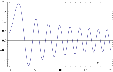
Figure 1: Plot of $e^{\pi\nu/2}K_{i\nu}(x)$ as a function of $\nu$ when $x=1$.

2. Derivation of the equation describing the large-$n$ zeros

We start with the asymptotic expansion of $K_{i\nu}(x)$ for $\nu\to+\infty$ given by [5] (see also [4, pp. 41–42])

$$e^{\pi\nu/2}K_{i\nu}(x)\sim\Re\,\sqrt{\frac{2\pi}{\nu\tanh\mu}}e^{i\Phi}\sum_{k=0}^{\infty}\frac{(\mbox{${\textstyle\frac{1}{2}}$})_{k}C_{k}(\mu)}{(\mbox{${\textstyle\frac{1}{2}}$}i\nu\tanh\mu)^{k}},$$ (2.1)

where

$$\Phi:=\nu(\mu-\tanh\mu)-\frac{\pi}{4},\quad\cosh\mu=\frac{\nu}{x}$$

and $(a)_{k}=\Gamma(a+k)/\Gamma(a)$ denotes the Pochhammer symbol. The first few coefficients $C_{k}(\mu)$ are

$$C_{0}(\mu)=1,\quad C_{1}(\mu)=-\frac{1}{8}+\frac{5\coth^{2}\mu}{24},\quad C_{2}(\mu)=\frac{3}{128}-\frac{77\coth^{2}\mu}{576}+\frac{385\coth^{4}\mu}{3456}~{};$$

values of $C_{k}(\mu)$ for $k\leq 5$ are derived in the appendix. It is important to point out that the determination of the expansion (2.1) from the integral (1.1) involves (when $\nu>x$) an infinite number of contributing saddle points. The expansion (2.1) results from the two dominant saddles, the remaining saddles yielding an exponentially small contribution of O$(e^{-\pi\nu})$. Then, from (2.1), the zeros of $K_{i\nu}(x)$ are given asymptotically by

$$\cos\Phi\biggl{\{}1-\frac{3C_{2}(\mu)}{(\nu\tanh\mu)^{2}}+\frac{105C_{4}(\mu)}{(\nu\tanh\mu)^{4}}+\cdots\biggr{\}}\hskip 142.26378pt$$

$$\hskip 113.81102pt+\sin\Phi\biggl{\{}\frac{C_{1}(\mu)}{\nu\tanh\mu}-\frac{15C_{3}(\mu)}{(\nu\tanh\mu)^{3}}+\frac{945C_{5}(\mu)}{(\nu\tanh\mu)^{5}}+\cdots\biggr{\}}=0.$$

Let

$$\Phi=(n+\mbox{${\textstyle\frac{1}{2}}$})\pi+\epsilon,$$ (2.2)

where $n$ is a large positive integer and $\epsilon$ is a small quantity. Then

$$\tan\epsilon={\displaystyle\frac{\frac{C_{1}(\mu)}{\nu\tanh\mu}-\frac{15C_{3}(\mu)}{(\nu\tanh\mu)^{3}}+\frac{945C_{5}(\mu)}{(\nu\tanh\mu)^{5}}+\cdots}{1-\frac{3C_{2}(\mu)}{(\nu\tanh\mu)^{2}}+\frac{105C^{4}(\mu)}{(\nu\tanh\mu)^{4}}+\cdots}}$$

$$=\frac{1}{\nu\tanh\mu}\biggl{\{}C_{1}(\mu)+\frac{3(C_{1}(\mu)C_{2}(\mu)-5C_{3}(\mu))}{(\nu\tanh\mu)^{2}}$$

$$+\frac{9C_{1}(\mu)C_{2}^{2}(\mu)-45C_{2}(\mu)C_{3}(\mu)-105C_{1}(\mu)C_{4}(\mu)+945C_{5}(\mu)}{(\nu\tanh\mu)^{4}}+\cdots\biggr{\}},$$

so that using $\arctan z=z-z^{3}/3+z^{5}/5-\ldots\,$ ($|z|<1$), we obtain

$$\epsilon=\frac{a_{0}(\mu)}{\nu}+\frac{a_{1}(\mu)}{\nu^{3}}+\frac{a_{2}(\mu)}{\nu^{5}}+\cdots,$$

where

$$a_{0}(\mu)=\frac{C_{1}(\mu)}{\tanh\mu},\qquad a_{1}(\mu)=\frac{3(C_{1}(\mu)C_{2}(\mu)-5C_{3}(\mu))-\frac{1}{3}C_{1}^{3}(\mu)}{\tanh^{3}\mu},$$

$$a_{2}(\mu)=\frac{1}{\tanh^{5}\mu}\biggl{\{}3(3C_{1}(\mu)C_{2}^{2}(\mu)-15C_{2}(\mu)C_{3}(\mu)-35(C_{1}(\mu)C_{4}(\mu)-9C_{5}(\mu)))$$

$$-3C_{1}^{2}(\mu)(C_{1}(\mu)C_{2}(\mu)-5C_{3}(\mu))+\frac{1}{5}C_{1}^{5}(\mu)\biggr{\}}.$$

Since $\tanh\mu=\sqrt{1-x^{2}/\nu^{2}}$, the coefficients $a_{k}(\mu)$ possess expansions in inverse powers of $\nu^{2}$. Some laborious algebra shows that

$$a_{0}(\mu) = \frac{1}{12}+\frac{x^{2}}{4\nu^{2}}+\frac{11x^{4}}{32\nu^{4}}+O(\nu^{-6})$$

$$a_{1}(\mu) = \frac{1}{360}-\frac{x^{2}}{4\nu^{2}}+O(\nu^{-4})$$

$$a_{2}(\mu) = \frac{1}{1260}+O(\nu^{-2}),$$

whence we obtain

$$\epsilon=\frac{1}{12\nu}+\frac{1}{\nu^{3}}\biggl{(}\frac{1}{360}+\frac{x^{2}}{4}\biggr{)}+\frac{1}{\nu^{5}}\biggl{(}\frac{1}{1260}-\frac{x^{2}}{4}+\frac{11x^{4}}{32}\biggr{)}+\cdots.$$ (2.3)

Making use of the expansion

$$\mu-\tanh\mu=\log\,\lambda\nu+\frac{x^{2}}{4\nu^{2}}+\frac{x^{4}}{32\nu^{4}}+\frac{x^{6}}{96\nu^{6}}+O(\nu^{-8}),\qquad\lambda:=\frac{2}{ex},$$

we then finally obtain from (2.2) and (2.3) the equation describing the large-$n$ zeros of $K_{i\nu}(x)$ given by

$$\nu\log\,\lambda\nu=m+\frac{A_{0}}{\nu}+\frac{A_{1}}{\nu^{3}}+\frac{A_{2}}{\nu^{5}}+\cdots,$$ (2.4)

where

$$A_{0}=\frac{1}{12}-\frac{x^{2}}{4},\quad A_{1}=\frac{1}{360}+\frac{x^{2}}{4}-\frac{x^{4}}{32},\quad A_{2}=\frac{1}{1260}-\frac{x^{2}}{4}+\frac{11x^{4}}{32}-\frac{x^{6}}{96}$$

and, for convenience, we have put $m:=(n+\mbox{${\textstyle\frac{3}{4}}$})\pi$.

3. Solution of the equation for the zeros

To solve (2.4) we expand $\nu$ as

$$\nu_{n}=\xi+\frac{c_{0}}{\xi}+\frac{c_{1}}{\xi^{3}}+\frac{c_{2}}{\xi^{5}}+\cdots,$$

where the $c_{k}$ are constants to be determined and we suppose that $\xi$ is large as $n\to\infty$. Substitution in (2.4) then produces

$$\xi\log\lambda\xi+\frac{c_{0}(1+\log\lambda\xi)}{\xi}+\frac{c_{1}(1+\log\lambda\xi)+\mbox{${\textstyle\frac{1}{2}}$}c_{0}^{2}}{\xi^{3}}+\frac{c_{2}(1+\log\lambda\xi)+c_{0}c_{1}-\mbox{${\textstyle\frac{1}{6}}$}c_{0}^{3}}{\xi^{5}}+\cdots$$

$$=m+\frac{A_{0}}{\xi}+\frac{A_{1}-A_{0}c_{0}}{\xi^{3}}+\frac{A_{2}-3A_{1}c_{0}+A_{0}(c_{0}^{2}-c_{1})}{\xi^{5}}+\cdots\,.$$

Equating coefficients of like powers of $\xi$, we obtain

$$\xi\log\lambda\xi=m,$$ (3.1)

and

$$c_{0}=\frac{A_{0}}{1+\log\lambda\xi},\quad c_{1}=\frac{A_{1}-A_{0}c_{0}-\mbox{${\textstyle\frac{1}{2}}$}c_{0}^{2}}{1+\log\lambda\xi},$$

$$c_{2}=\frac{A_{2}-3A_{1}c_{0}+A_{0}(c_{0}^{2}-c_{1})-c_{0}c_{1}+\mbox{${\textstyle\frac{1}{6}}$}c_{0}^{3}}{1+\log\lambda\xi}~{}.$$

The solution of (3.1) for the lowest-order term $\xi$ can be expressed in terms of the Lambert $W$ function, which is the (positive) solution of $W(z)e^{W(z)}=z$ for $z>0$. Rearrangement of (3.1) shows that

$$\frac{m}{\xi}\,e^{m/\xi}=\lambda m,$$

whence

$$\xi=\frac{m}{W(\lambda m)}.$$ (3.2)

The asymptotic expansion of $W(z)$ for $z\to+\infty$ is [2], [3, (4.13.10)]

$$W(z)\sim L_{1}-L_{2}+\frac{L_{2}}{L_{1}}+\frac{L_{2}^{2}-2L_{2}}{2L_{1}^{2}}+\frac{(6-9L_{2}+2L_{2}^{2})L_{2}}{6L_{1}^{3}}+\frac{(-12+36L_{2}-22L_{2}^{2}+3L_{2}^{3})L_{2}}{12L_{1}^{4}}+\cdots,$$

where $L_{1}=\log z$, $L_{2}=\log\log z$, from which it follows that

$$\frac{1}{W(z)}\sim\frac{1}{L_{1}}\biggl{\{}1+\frac{L_{2}}{L_{1}}+\frac{L_{2}(L_{2}-1)}{L_{1}^{2}}+\frac{(1-5L_{2}+2L_{2}^{2})L_{2}}{2L_{1}^{3}}+\frac{(-6+21L_{2}-26L_{2}^{2}+6L_{2}^{3})L_{2}}{6L_{1}^{4}}+\cdots\biggr{\}}.$$

Then we have the expansion for $\xi$ as $\lambda m\to\infty$ given by

$$\xi\sim\frac{m}{\log\lambda m}\biggl{\{}1+\frac{\log\log\lambda m}{\log\lambda m}+\frac{\log\log\lambda m(\log\log\lambda m-1)}{(\log\lambda m)^{2}}+\cdots\biggr{\}},$$ (3.3)

where we recall that $m=(n+\mbox{${\textstyle\frac{3}{4}}$})\pi$.

If we define $\chi:=\xi/m$, so that by (3.1) $1+\log\lambda\xi=(1+\chi)/\chi$ and introduce the coefficients

$$B_{0}=\frac{A_{0}}{1+\chi},\quad B_{1}=\frac{A_{1}-A_{0}c_{0}-\mbox{${\textstyle\frac{1}{2}}$}c_{0}^{2}}{\chi^{2}(1+\chi)},\quad B_{2}=\frac{A_{2}-3A_{1}c_{0}+A_{0}(c_{0}^{2}-c_{1})-c_{0}c_{1}+\mbox{${\textstyle\frac{1}{6}}$}c_{0}^{3}}{\chi^{4}(1+\chi)},$$ (3.4)

then we finally have the result:

Theorem 1

$\!\!\!.$  The expansion for the $n$th $\nu$-zero of $K_{\i\nu}(x)$ for fixed $x>0$ is

$$\nu_{n}\sim\frac{m}{W(\lambda m)}+\frac{B_{0}}{m}+\frac{B_{1}}{m^{3}}+\frac{B_{2}}{m^{5}}+\cdots\qquad(n\to\infty),$$ (3.5)

where $m=(n+\mbox{${\textstyle\frac{3}{4}}$})\pi$, $\lambda=2/(ex)$ and the coefficients $B_{k}$ are given in (3.4).

The leading form of $\xi$ from (3.3) is, with $\lambda=2/(ex)$,

$$\xi\sim\frac{(n+\mbox{${\textstyle\frac{3}{4}}$})\pi}{\log(n+\mbox{${\textstyle\frac{3}{4}}$})\pi+\log\lambda}\qquad(n\to\infty),$$

which yields the approximate estimate in (1.2). In numerical calculations it is found more expedient to use the expression for $\xi$ in terms of the Lambert function in (3.2), rather than (3.3), since the asymptotic scale in this latter series is $\log\lambda m$ and so requires an extremely large value of $n$ to attain reasonable accuracy.

We present numerical results in Table 1 showing the zeros of $K_{i\nu}(x)$ computed using the FindRoot command in Mathematica compared with the asymptotic values determined from the expansion (3.5) with coefficients $B_{k}$, $k\leq 2$, where $\xi$ is evaluated from (3.2). The value of the zeroth-order approximation $\xi=m/W(\lambda m)$ is shown in the final column. It is seen that there is excellent agreement with the computed zeros, even for $n=1$.

Table 1: Values of the zeros of $K_{i\nu}(x)$ and their asymptotic estimates when $x=1$.

$n$	$\nu_{n}$	Asymptotic	$\xi$
1	4.5344907181	4.5345024086	4.550063
2	5.8798671997	5.8798689800	5.890918
4	8.2589364092	8.2589365588	8.265990
5	9.3550938258	9.3550938860	9.361083
10	14.3318529171	14.3318529198	14.335296
15	18.8230418511	18.8230418514	18.825473
20	23.0318794957	23.0318794958	23.033764
30	30.9169674670	30.9169674670	30.918273

Appendix: The coefficients $C_{k}(\mu)$ in the expansion (2.1)

The integral in (1.1) can be cast in the form

$$K_{i\nu}(x)=\frac{1}{2}\int_{-\infty}^{\infty}e^{-x\psi(t)}dt,\qquad\psi(t):=\cosh t-it\cosh\mu,$$ (A.1)

where $\cosh\mu=\nu/x$. In the right-half plane, the dominant saddle point (where $\psi^{\prime}(t)=0$) is situated at $t_{0}=\mu+\mbox{${\textstyle\frac{1}{2}}$}\pi i$, with a similar saddle in the left-half plane at $-\mu+\mbox{${\textstyle\frac{1}{2}}$}\pi i$. When $\nu>x$, there are in addition two infinite strings of subdominant saddles at $\pm\mu+(2k+\mbox{${\textstyle\frac{1}{2}}$})\pi i$ ($k=1,2,\ldots$) parallel to the positive imaginary axis over which the integration path in (A.1) is deformed; see [5], [4, pp. 41–42] for details.

We introduce the new variable $w$ by

$$w^{2}=\psi(t)-\psi(t_{0})=\frac{1}{2}i\sinh\mu\,(t-t_{0})^{2}+\frac{1}{6}i\cosh\mu\,(t-t_{0})^{3}+\frac{1}{24}i\sinh\mu\,(t-t_{0})^{4}+\cdots$$

to find with the help of Mathematica using the InverseSeries command (essentially Lagrange inversion)

$$t-t_{0}=e^{-\pi i/4}\sqrt{\frac{2}{\sinh\mu}}\,w+\frac{i\coth\mu}{2\sinh\mu}\,w^{2}-ie^{-\pi i/4}\sqrt{\frac{2}{\sinh\mu}}\,\frac{(-3+5\coth^{2}\mu)}{36\sinh\mu}\,w^{3}+\cdots.$$

Differentiation then yields the expansion

$$\frac{dt}{dw}\stackrel{{\scriptstyle e}}{{=}}e^{-\pi i/4}\sqrt{\frac{2}{\sinh\mu}}\,\sum_{k\geq 0}\frac{C_{k}(\mu)}{(\mbox{${\textstyle\frac{1}{2}}$}i\sinh\mu)^{k}}\,w^{2k},$$ (A.2)

where $\stackrel{{\scriptstyle e}}{{=}}$ signifies the inclusion of only the even powers of $w$, since odd powers will not enter into this calculation. The first few coefficients are found to be:

$$C_{0}(\mu)=1,\qquad C_{1}(\mu)=-\frac{1}{8}+\frac{5\coth^{2}\mu}{24},$$

$$C_{2}(\mu)=\frac{3}{128}-\frac{77\coth^{2}\mu}{576}+\frac{385\coth^{4}\mu}{3456},$$

$$C_{3}(\mu)=-\frac{5}{1024}+\frac{1521\coth^{2}\mu}{25600}-\frac{17017\coth^{4}\mu}{138240}+\frac{17017\coth^{6}\mu}{248832},$$

$$C_{4}(\mu)=\frac{35}{32768}-\frac{96833\coth^{2}\mu}{4300800}+\frac{144001\coth^{4}\mu}{1720320}-\frac{1062347\coth^{6}\mu}{9953280}+\frac{1062347\coth^{8}\mu}{23887872},$$

$$C_{5}(\mu)=-\frac{63}{262144}+\frac{67608983\coth^{2}\mu}{8670412800}-\frac{35840233\coth^{4}\mu}{796262400}+\frac{3094663\coth^{6}\mu}{31850496}$$

$$-\frac{154040315\coth^{8}\mu}{1719926784}+\frac{154040315\coth^{10}\mu}{5159780352}.$$ (A.3)

Then the integral (A.1) resulting from the saddle $t_{0}$ can be expressed as

$$\int_{-\infty}^{\infty}e^{-xw^{2}}\,\frac{dt}{dw}\,dw,$$

which, after substitution of the expansion (A.2) followed by routine integration and taking into account the contribution from the saddle at $t=-\mu+\mbox{${\textstyle\frac{1}{2}}$}\pi i$, then yields the expansion for $K_{i\nu}(x)$ stated in (2.1).

References

• [1] S.M. Bagirova and A. Kh. Khanmamedov, On zeros of the modified Bessel function of the second kind, Comput. Math. and Math. Phys. 60 (2020) 817–820.
• [2] R.M. Corless, G.H. Gonnet, D.E.G. Hare, D.J. Jeffrey and D.E. Knuth, On the Lambert $W$ function, Adv. in Comp. Math. 5 (1996) 329–359.
• [3] F.W.J. Olver, D.W. Lozier, R.F. Boisvert and C.W. Clark (eds.), NIST Handbook of Mathematical Functions, Cambridge University Press, Cambridge, 2010.
• [4] R.B. Paris, Hadamard Expansions and Hyperasymptotic Evaluation, Encyclopedia of Mathematics and its Applications Vol. 141, Cambridge University Press, Cambridge, 2011.
• [5] N.M. Temme, Steepest descent paths for integrals defining the modified Bessel functions of imaginary order, Methods Appl. Anal. 1 (1994) 14–24.