Semileptonic $\Xi_{c}$ baryon decays in the light cone QCD sum rules

Abstract

Form factors of the weak $\Xi_{c}\to\Xi(\Lambda)$ transitions are calculated within the light cone QCD sum rules. The pollutions coming from the contribution of the negative parity $\Xi_{c}^{*}$ baryon is eliminated by considering the combinations of sum rules corresponding to the different Lorentz structures. Having obtained the form factors, the branching ratios of the $\Xi_{c}\to\Xi(\Lambda)\ell\nu$ decays are also calculated, and our predictions are compared with the results of other approaches as well as the measurements done by BELLE and ALICE Collaborations.

I Introduction

The electroweak decays of the heavy flavored hadrons provide useful information about the helicity structure of the effective Hamiltonian and the matrix elements of the Cabibbo–Kobayashi–Maskawa matrix (CKM). These decays are also very promising in looking for new physics searches. For these goals, the semileptonic decays of the heavy mesons and baryons provide an ideal research area. Since the leptonic part of these transitions is well known, all probable complications can be attributed to the hadronic matrix element. The study of the semileptonic $\Xi_{c}\to B(B=\Xi\,{\rm or}\,\Lambda)\ell\nu$ decays that are induced by the $c\to s$ and $c\to d$ transitions are helpful for precise determination of the values of the CKM matrix elements $V_{cs}$ and $V_{cd}$ . Moreover, these decays can also be used to test the predictions of the heavy quark effective theory.

The form factors also play a crucial role in the theoretical analysis of the non-leptonic decays of the baryons and might also be useful for the study of CP violation.

Significant experimental progress on the semileptonic decays of $\Xi_{c}$ baryon has been achieved recently. Belle Collaboration reported the measurement of the branching ratios of the semileptonic decays $\Xi_{c}^{0}\to\Xi^{-}\ell^{+}\nu$ Li et al. (2021),

$$B(\Xi_{c}^{0}\to\Xi^{-}e^{+}\nu_{e}) = (1.72\pm 0.10\pm 0.12\pm 0.50)\%~{},$$

$$B(\Xi_{c}^{0}\to\Xi^{-}\mu^{+}\nu_{\mu}) = (1.71\pm 0.17\pm 0.13\pm 0.50)\%~{}.$$

Moreover, ALICE Collaboration has also announced the result for the branching ratio of the $\Xi_{c}^{0}\to\Xi^{-}\ell\nu$ transition ($B=(1.8\pm 0.2)\%$) Acharya et al. (2021), which agrees with BELLE’s measurement within error ranges.

The semileptonic decays of the $\Xi_{c}$ baryon have been comprehensively studied in the framework of different approaches, such as the light–front formalism Geng et al. (2018, 2019), relativistic quark model Faustov and Galkin (2019), lattice QCD Zhang et al. (2021), 3–point QCD sum rules Zhao (2021), and light cone QCD sum rules method Azizi et al. (2012).

In this study, we calculated the form factors and branching ratios of the semileptonic decay of $\Xi_{c}$ within the LCSR framework. It should be noted that the same channel was already studied in Azizi et al. (2012). However, the prediction of the branching ratio obtained in that study is considerably larger than the results of the other approaches as well as experimental measurements. This study also aims to understand the source of this discrepancy. In our opinion, the reason for the discrepancy can be attributed to the fact that the interpolating current for the given heavy baryon couples not only to the ground state baryon with positive parity $J^{P}=\frac{1}{2}^{+}$ but also to a heavier baryon with negative parity $J^{P}=\frac{1}{2}^{-}$. Hence, the dispersion relation of the $\Xi_{c}$ baryon gets modified when the contribution of the negative parity $\Xi_{c}$ baryon is taken into account, which is $300~{}MeV$ heavier compared to the ground state $\Xi_{c}$ baryon. In the light of new experimental data, we reanalyze the semileptonic decays of $\Xi_{b}\rightarrow\Xi(\Lambda)l\nu$ within light-cone sum rules in detail by taking into account the contributions of $J^{P}={1\over 2}^{-}$ heavy baryon.

So far, the light cone sum rules (LCSR) have successfully been applied to the wide range of problems of the hadronic physics, such as nucleon electromagnetic form factor Braun et al. (2006), form factors and strong coupling constants of the heavy baryons Khodjamirian et al. (2011), rare $\Lambda_{b}\to N(N^{\ast})\ell^{+}\ell^{-}$ decays Aliev et al. (2015), etc.

The paper is organized as follows. In Section II, the light cone sum rules (LCSR) for the $\Xi_{c}\to B(\Xi~{}\mbox{or}~{}\Lambda)$ transition form factors are derived. In Section III, the numerical analysis of the transition form factors is performed. This section also contains our predictions on the decay widths of the $\Xi_{c}\to B\ell\nu$ transitions. Finally, we compare our results on the branching ratios with those predicted by the other approaches.

II The LCSR for the $\Xi_{c}\to B$ transition form factors

$\Xi_{c}\to B(\Xi~{}\mbox{or}~{}\Lambda)$ decay is induced by the $c\to s(d)$ transition. The matrix elements induced by the vector and axial-vector transition currents are described with the help of the three form factors,

$$\langle\Xi_{c}(p-q)|\bar{q}\gamma_{\mu}c|B(p)\rangle=\bar{u}_{\Xi_{c}}(p-q)\Big{[}f_{1}(q^{2})\gamma_{\mu}+{i}\frac{f_{2}(q^{2})}{m_{\Xi_{c}}}\sigma_{\mu\nu}q^{\nu}+\frac{f_{3}(q^{2})}{m_{\Xi_{c}}}q^{\mu}\Big{]}u_{B}(p)~{},$$ (1)

$$\langle\Xi_{c}(p-q)|\bar{q}\gamma_{\mu}\gamma_{5}c|B(p)\rangle=\bar{u}_{\Xi_{c}}(p-q)\Big{[}g_{1}(q^{2})\gamma_{\mu}+{i}\frac{g_{2}(q^{2})}{m_{\Xi_{c}}}\sigma_{\mu\nu}q^{\nu}+\frac{g_{3}(q^{2})}{m_{\Xi_{c}}}q^{\mu}\Big{]}\gamma_{5}u_{B}(p)~{}.$$ (2)

The form factors responsible for the $\Xi_{c}^{\ast}\to B$ transition can be obtained from Eqs. (1) and (2) with the replacements $f_{i}\to\widetilde{f}_{i}$, $g_{i}\to\widetilde{g}_{i}$, inserting the Dirac matrix $\gamma_{5}$ after the $\Xi_{c}$ baryon bispinor, and replacing $\Xi_{c}$ with $\Xi_{c}^{\ast}$.

In order to derive the LCSR for the form factors, we start by considering the following correlation function(s),

$$\Pi^{V(A)}_{\mu}(p,q)=i\int d^{4}xe^{iqx}\langle 0|T\{\eta_{{}_{\Xi_{c}}}(0)J_{\mu}^{V(A)}(x)\}|B(p)\rangle~{},$$ (3)

where $\eta_{{}_{\Xi_{c}}}$ is the interpolating current of the $\Xi_{c}$ baryon, and $J_{\mu}^{V(A)}=\bar{c}\gamma_{\mu}q(\bar{c}\gamma_{\mu}\gamma_{5}q)$ are the transition currents. In further calculations, we use the general form of the interpolating current $\Xi_{c}$, Bagan et al. (1992).

$$\eta_{{}_{\Xi_{c}}} = \frac{1}{\sqrt{6}}\epsilon_{abc}\Big{\{}\vphantom{\int_{0}^{x_{2}}}2[q^{aT}(x)Cs^{b}(x)]\gamma_{5}c^{c}(x)+[q^{aT}(x)Cc^{b}(x)]\gamma_{5}s^{c}(x)+[c^{aT}(x)Cs^{b}(x)]\gamma_{5}q^{c}(x)$$ (4)

$$+ 2\beta[u^{aT}(x)C\gamma_{5}s^{b}(x)]c^{c}(x)+\beta[q^{aT}(x)C\gamma_{5}c^{b}(x)]s^{c}(x)+\beta[c^{aT}(x)C\gamma_{5}s^{b}(x)]q^{c}(x)\Big{\}}~{}.$$

Here $q$ is the light quark, $C$ is the charge conjugation operator, $a,~{}b$ and $c$ are the color indices, and $\beta$ is an arbitrary parameter, and $\beta=-1$ corresponds to the Ioffe current.

To derive the LCSR for the transition form factors, we first calculate the hadronic part of the correlation function, which is achieved by inserting the full set of charmed–baryon states between the interpolating current $\eta_{{}_{\Xi_{c}}}$ and the transition current $J_{\mu}$ in Eq. (3). Thus, the hadronic part contains the contributions of the lowest positive–parity $\Xi_{c}$, as well as its negative–parity partner $\Xi_{c}^{\ast}$, i.e.,

$$\Pi_{\mu}^{V(A)}(p,q)=\sum_{i}\frac{\langle 0|\eta_{{}_{\Xi_{c}}}(0)|\Xi_{c}^{i}(p-q,s)\rangle\langle\Xi_{c}^{i}(p-q,s)|\bar{c}\gamma_{\mu}q(\bar{c}\gamma_{\mu}\gamma_{5}q)|B(p)\rangle}{m_{i}^{2}-(p-q)^{2}}+\cdots~{},$$ (5)

where $\cdots$ denote the contributions of all excited and continuum states with the quantum numbers of $\Xi_{c}$, and summation is performed over the ground and first orbital excited states. The first term in the right hand side of the Eq. (5) describes the coupling of the $\Xi_{c}(\Xi_{c}^{\ast})$ baryon with the interpolating current $\eta_{{}_{\Xi_{c}}}$ which is defined as,

$$\langle 0|\eta_{{}_{\Xi_{c}}}(0)|\Xi_{c}(p-q,s)\rangle = \lambda_{{}_{\Xi_{c}}}u_{{}_{\Xi_{c}}}(p-q)~{},$$

$$\langle 0|\eta_{{}_{\Xi_{c}^{\ast}}}(0)|\Xi_{c}^{\ast}(p-q,s)\rangle = \lambda_{{}_{\Xi_{c}^{\ast}}}\gamma_{5}u_{{}_{\Xi_{c}^{\ast}}}(p-q)~{}.$$ (6)

where $\lambda_{{}_{\Xi_{c}}}(\lambda_{{}_{\Xi_{c}^{\ast}}})$ is the residue of the corresponding baryon.

Using the definitions of the transition form factors for the vector transition current, and using the Dirac equation $\not\!pu_{B}(p)=m_{B}u_{B}(p)$ we get,

$$\Pi_{\mu}^{V}(p,q) = \frac{\lambda_{{}_{\Xi_{c}}}}{m_{{}_{\Xi_{c}}}^{2}-(p-q)^{2}}\Bigg{\{}f_{1}(q^{2})\Big{[}2p_{\mu}+(m_{{}_{\Xi_{c}}}-m_{B})\gamma_{\mu}-2q_{\mu}+\gamma_{\mu}\not\!q\Big{]}$$ (7)

$$- \frac{f_{2}(q^{2})}{m_{{}_{\Xi_{c}}}}\Big{[}2p_{\mu}\not\!q+(m_{{}_{\Xi_{c}}}^{2}-m_{B}^{2})\gamma_{\mu}+(m_{{}_{\Xi_{c}}}+m_{B})\gamma_{\mu}\not\!q-(m_{{}_{\Xi_{c}}}+m_{B})q_{\mu}-q_{\mu}\not\!q\Big{]}$$

$$+ \frac{f_{3}(q^{2})}{m_{{}_{\Xi_{c}}}}(m_{{}_{\Xi_{c}}}+m_{B}-\not\!q)q_{\mu}\Bigg{\}}u_{B}(p)$$

$$+ \frac{\lambda_{{}_{\Xi_{c}^{\ast}}}}{m_{{}_{\Xi_{c}^{\ast}}}^{2}-(p-q)^{2}}\Bigg{\{}\widetilde{f}_{1}(q^{2})\Big{[}-2p_{\mu}+(m_{{}_{\Xi_{c}^{\ast}}}+m_{B})\gamma_{\mu}+2q_{\mu}-\gamma_{\mu}\not\!q\Big{]}$$

$$+ \frac{\widetilde{f}_{2}(q^{2})}{m_{{}_{\Xi_{c}^{\ast}}}}\Big{[}2p_{\mu}\not\!q+(m_{{}_{\Xi_{c}^{\ast}}}^{2}-m_{B}^{2})\gamma_{\mu}-(m_{{}_{\Xi_{c}^{\ast}}}-m_{B})\gamma_{\mu}\not\!q+(m_{{}_{\Xi_{c}^{\ast}}}-m_{B})q_{\mu}-q_{\mu}\not\!q\Big{]}$$

$$+ \frac{\widetilde{f}_{3}(q^{2})}{m_{{}_{\Xi_{c}^{\ast}}}}(m_{\_{\Xi_{c}^{\ast}}}-m_{B}+\not\!q)q_{\mu}\Bigg{\}}u_{B}(p)~{}.$$

$\Pi_{\mu}^{A}(p,q)$ can easily be obtained from $\Pi_{\mu}^{V}(p,q)$ by making the replacements $\Big{(}f_{i}\to g_{i};~{}\widetilde{f}_{i}\to\widetilde{g}_{i};~{}m_{B}\to-m_{B}\Big{)}$, and multiplying $\gamma_{5}$ matrix to the right end, i.e.,

$$\Pi_{\mu}^{A}(p,q) = \Pi_{\mu}^{V}(p,q)\Big{(}f_{i}\to g_{i};~{}\widetilde{f}_{i}\to\widetilde{g}_{i};~{}m_{B}\to-m_{B}\Big{)}\gamma_{5}~{}.$$

We now turn our attention to the calculation of the correlation function (3) for the $\Xi_{c}(\Xi_{c}^{\ast})\to B$ transition. We take $(p-q)^{2},q^{2}\ll m_{{}_{\Xi_{c}}}^{2}$ to justify the expansion of the product of the two currents in the correlation function (3) near the light cone $x^{2}\approx 0$,hence, the matrix element $\varepsilon^{abc}\left<0|q_{\alpha}^{a}(0)s_{\beta}^{b}(0)s_{\gamma}^{c}(0)|B(p)\right>$ is obtained. This matrix element is parametrized in terms of the $\Xi$ and $\Lambda$ baryon distribution amplitudes (DAs) of a different twist. The explicit expressions of the $\Xi$ and $\Lambda$ baryon DAs can be found in Liu and Huang (2009a, b); Wein and Schäfer (2015). The operator product expansion is obtained by convolution of the hard–scattering amplitudes formed by the virtual c–quark propagator and the $\Xi(\Lambda)$ baryon DAs with increasing twists. In our calculations, we take into account all three particle B–baryon DAs up to twist–6. However, we neglect the contributions of the four-particle (quark and gluon) DAs.

Matching the coefficient of the relevant Lorentz structures in both representations of the correlation function, we get the sum rules for the transition form factors. Finally, we perform Borel transformation over $-(p-q)^{2}$ in order to suppress the higher state and continuum contributions and obtain the following sum rules for the form factors of the $\bar{c}\gamma_{\mu}s$ transition current,

$$\Pi_{1}^{B}(p,q) = 2\lambda_{{}_{\Xi_{c}}}f_{1}(q^{2})e^{-m_{{}_{\Xi_{c}}}^{2}/M^{2}}-2\lambda_{{}_{\Xi_{c}^{\ast}}}\widetilde{f}_{1}(q^{2})e^{-m_{{}_{\Xi_{c}^{\ast}}}^{2}/M^{2}},$$

$$\Pi_{2}^{B}(p,q) = -2\lambda_{{}_{\Xi_{c}}}\frac{f_{2}(q^{2})}{m_{{}_{\Xi_{c}}}}e^{-m_{{}_{\Xi_{c}}}^{2}/M^{2}}+2\lambda_{{}_{\Xi_{c}^{\ast}}}\frac{\widetilde{f}_{2}(q^{2})}{m_{{}_{\Xi_{c}^{\ast}}}}e^{-m_{{}_{\Xi_{c}^{\ast}}}^{2}/M^{2}},$$

$$\Pi_{3}^{B}(p,q) = \lambda_{{}_{\Xi_{c}}}e^{-m_{{}_{\Xi_{c}}}^{2}/M^{2}}\Big{(}f_{1}(q^{2})-\frac{f_{2}(q^{2})}{m_{{}_{\Xi_{c}}}}(m_{{}_{\Xi_{c}}}+m_{B})\Big{)}$$

$$+ \lambda_{{}_{\Xi_{c}^{\ast}}}e^{-m_{{}_{\Xi_{c}^{\ast}}}^{2}/M^{2}}\Big{(}-\widetilde{f}_{1}(q^{2})-\frac{\widetilde{f}_{2}(q^{2})}{m_{{}_{\Xi_{c}^{\ast}}}}(m_{{}_{\Xi_{c}^{\ast}}}-m_{B})\Big{)},$$

$$\Pi_{4}^{B}(p,q) = \lambda_{{}_{\Xi_{c}}}e^{-m_{{}_{\Xi_{c}}}^{2}/M^{2}}\Big{(}(m_{{}_{\Xi_{c}}}-m_{B})(f_{1}(q^{2})-\frac{f_{2}(q^{2})}{m_{{}_{\Xi_{c}}}}(m_{{}_{\Xi_{c}}}+m_{B}))\Big{)}$$

$$+ \lambda_{{}_{\Xi_{c}^{\ast}}}e^{-m_{{}_{\Xi_{c}^{\ast}}}^{2}/M^{2}}\Big{(}(m_{{}_{\Xi_{c}^{\ast}}}+m_{B})(\widetilde{f}_{1}(q^{2})+\frac{\widetilde{f}_{2}(q^{2})}{m_{{}_{\Xi_{c}^{\ast}}}}(m_{{}_{\Xi_{c}^{\ast}}}-m_{B}))\Big{)},$$

$$\Pi_{5}^{B}(p,q) = \lambda_{{}_{\Xi_{c}}}e^{-m_{{}_{\Xi_{c}}}^{2}/M^{2}}\Big{(}-2f_{1}(q^{2})+\frac{(f_{2}(q^{2})+f_{3}(q^{2}))}{m_{{}_{\Xi_{c}}}}(m_{{}_{\Xi_{c}^{\ast}}}+m_{B})\Big{)}$$

$$+ \lambda_{{}_{\Xi_{c}^{\ast}}}e^{-m_{{}_{\Xi_{c}^{\ast}}}^{2}/M^{2}}\Big{(}2\widetilde{f}_{1}(q^{2})+\frac{(\widetilde{f}_{2}(q^{2})+\widetilde{f}_{3}(q^{2}))}{m_{{}_{\Xi_{c}^{\ast}}}}(m_{{}_{\Xi_{c}^{\ast}}}-m_{B})\Big{)},$$

$$\Pi_{6}^{B}(p,q) = \frac{\lambda_{{}_{\Xi_{c}}}}{m_{{}_{\Xi_{c}}}}e^{-m_{{}_{\Xi_{c}}}^{2}/M^{2}}\Big{(}f_{2}(q^{2})-f_{3}(q^{2})\Big{)}-\frac{\lambda_{{}_{\Xi_{c}^{\ast}}}}{m_{{}_{\Xi_{c}^{\ast}}}}e^{-m_{{}_{\Xi_{c}^{\ast}}}^{2}/M^{2}}\Big{(}\widetilde{f}_{2}(q^{2})-\widetilde{f}_{3}(q^{2})\Big{)}.$$ (8)

Here, $\Pi_{1}^{B}(p,q)$, $\Pi_{2}^{B}(p,q)$, $\Pi_{3}^{B}(p,q)$, $\Pi_{4}^{B}(p,q)$, $\Pi_{5}^{B}(p,q)$, and $\Pi_{6}^{B}(p,q)$ are the invariant functions for the Lorentz structures, $p_{\mu}$, $p_{\mu}\!\!\not\!q$,$\gamma_{\mu}\!\!\not\!q$, $\gamma_{\mu}$, $q_{\mu}$, and $q_{\mu}\!\!\not\!q$ structures, respectively.

Note that, the equations for the axial vector current, $\gamma_{\mu}\gamma_{5}$, can be obtained from Eq. (II) by making the following replacements $f_{i}\to-g_{i}$, $\widetilde{f}_{i}\to-\widetilde{g}_{i}$, $m_{B}\to-m_{B}$, and $\Pi_{i}^{(V)B}\to\Pi_{i}^{(A)B}$.

Solving the six equations given in (II) we obtain the LCSR for the transition form factors $f_{i}$, $\widetilde{f}_{i}$ for vector current and $g_{i}$, and $\widetilde{g}_{i}$ for axial vector which read as:

$$f_{1} = {e^{m_{\Xi_{c}}^{2}/M^{2}}\over 2\lambda_{\Xi_{c}}(m_{{}_{\Xi_{c}^{\ast}}}+m_{{}_{\Xi_{c}}})}\Big{\{}(m_{{}_{\Xi_{c}}}+m_{B})\Big{[}\Pi_{1}^{(V)B}-(m_{{}_{\Xi_{c}^{\ast}}}-m_{B})\Pi_{2}^{(V)B}\Big{]}+2(m_{{}_{\Xi_{c}^{\ast}}}-m_{{}_{\Xi_{c}}})\Pi_{3}^{(V)B}+2\Pi_{4}^{(V)B}\Big{\}}~{},$$

$$f_{2} = {m_{{}_{\Xi_{c}}}e^{m_{\Xi_{c}}^{2}/M^{2}}\over 2\lambda_{\Xi_{c}}(m_{{}_{\Xi_{c}^{\ast}}}+m_{{}_{\Xi_{c}}})}\Big{[}\Pi_{1}^{(V)B}-(m_{{}_{\Xi_{c}^{\ast}}}-m_{B})\Pi_{2}^{(V)B}-2\Pi_{3}^{(V)B}\Big{]}~{},$$

$$f_{3} = {m_{{}_{\Xi_{c}}}e^{m_{\Xi_{c}}^{2}/M^{2}}\over 2\lambda_{\Xi_{c}}(m_{{}_{\Xi_{c}^{\ast}}}+m_{{}_{\Xi_{c}}})}\Big{[}\Pi_{1}^{(V)B}+2(\Pi_{3}^{(V)B}+\Pi_{5}^{(V)B})-(m_{{}_{\Xi_{c}^{\ast}}}-m_{B})(\Pi_{2}^{(V)B}+2\Pi_{6}^{(V)B})\Big{]}~{},$$

$$\widetilde{f}_{1} = {-e^{m_{\Xi_{c}^{\ast}}^{2}/M^{2}}\over 2\lambda_{\Xi_{c}^{\ast}}(m_{{}_{\Xi_{c}^{\ast}}}+m_{{}_{\Xi_{c}}})}\Big{\{}(m_{{}_{\Xi_{c}^{\ast}}}-m_{B})\Big{[}\Pi_{1}^{(V)B}+(m_{{}_{\Xi_{c}}}+m_{B})\Pi_{2}^{(V)B}\Big{]}-2(m_{{}_{\Xi_{c}^{\ast}}}-m_{{}_{\Xi_{c}}})\Pi_{3}^{(V)B}-2\Pi_{4}^{(V)B}\Big{\}}~{},$$

$$\widetilde{f}_{2} = {m_{{}_{\Xi_{c}^{\ast}}}e^{m_{\Xi_{c}^{\ast}}^{2}/M^{2}}\over 2\lambda_{\Xi_{c}^{\ast}}(m_{{}_{\Xi_{c}^{\ast}}}+m_{{}_{\Xi_{c}}})}\Big{[}\Pi_{1}^{(V)B}+(m_{{}_{\Xi_{c}}}+m_{B})\Pi_{2}^{(V)B}-2\Pi_{3}^{(V)B}\Big{]}~{},$$

$$\widetilde{f}_{3} = {m_{{}_{\Xi_{c}^{\ast}}}e^{m_{\Xi_{c}^{\ast}}^{2}/M^{2}}\over 2\lambda_{\Xi_{c}^{\ast}}(m_{{}_{\Xi_{c}^{\ast}}}+m_{{}_{\Xi_{c}}})}\Big{[}\Pi_{1}^{(V)B}+2(\Pi_{3}^{(V)B}+\Pi_{5}^{(V)B})+(m_{{}_{\Xi_{c}}}+m_{B})(\Pi_{2}^{(V)B}+2\Pi_{6}^{(V)B})\Big{]}~{},$$

$$g_{1} = {-e^{m_{\Xi_{c}}^{2}/M^{2}}\over 2\lambda_{\Xi_{c}}(m_{{}_{\Xi_{c}^{\ast}}}+m_{{}_{\Xi_{c}}})}\Big{\{}(m_{{}_{\Xi_{c}}}-m_{B})\Big{[}\Pi_{1}^{(A)B}-(m_{{}_{\Xi_{c}^{\ast}}}+m_{B})\Pi_{2}^{(A)B}\Big{]}+2(m_{{}_{\Xi_{c}^{\ast}}}-m_{{}_{\Xi_{c}}})\Pi_{3}^{(A)B}+2\Pi_{4}^{(A)B}\Big{\}}~{},$$

$$g_{2} = {-m_{{}_{\Xi_{c}}}e^{m_{\Xi_{c}}^{2}/M^{2}}\over 2\lambda_{\Xi_{c}}(m_{{}_{\Xi_{c}^{\ast}}}+m_{{}_{\Xi_{c}}})}\Big{[}\Pi_{1}^{(A)B}-(m_{{}_{\Xi_{c}^{\ast}}}+m_{B})\Pi_{2}^{(A)B}-2\Pi_{3}^{(A)B}\Big{]}~{},$$

$$g_{3} = {-m_{{}_{\Xi_{c}}}e^{m_{\Xi_{c}}^{2}/M^{2}}\over 2\lambda_{\Xi_{c}}(m_{{}_{\Xi_{c}^{\ast}}}+m_{{}_{\Xi_{c}}})}\Big{[}\Pi_{1}^{(A)B}+2(\Pi_{3}^{(A)B}+\Pi_{5}^{(A)B})-(m_{{}_{\Xi_{c}^{\ast}}}+m_{B})(\Pi_{2}^{(A)B}+2\Pi_{6}^{(A)B})\Big{]}~{},$$

$$\widetilde{g}_{1} = {e^{m_{\Xi_{c}^{\ast}}^{2}/M^{2}}\over 2\lambda_{\Xi_{c}^{\ast}}(m_{{}_{\Xi_{c}^{\ast}}}+m_{{}_{\Xi_{c}}})}\Big{\{}(m_{{}_{\Xi_{c}^{\ast}}}+m_{B})\Big{[}\Pi_{1}^{(A)B}+(m_{{}_{\Xi_{c}}}-m_{B})\Pi_{2}^{(A)B}\Big{]}-2(m_{{}_{\Xi_{c}^{\ast}}}-m_{{}_{\Xi_{c}}})\Pi_{3}^{(A)B}-2\Pi_{4}^{(A)B}\Big{\}}~{},$$

$$\widetilde{g}_{2} = {-m_{{}_{\Xi_{c}^{\ast}}}e^{m_{\Xi_{c}^{\ast}}^{2}/M^{2}}\over 2\lambda_{\Xi_{c}^{\ast}}(m_{{}_{\Xi_{c}^{\ast}}}+m_{{}_{\Xi_{c}}})}\Big{[}\Pi_{1}^{(A)B}+(m_{{}_{\Xi_{c}}}-m_{B})\Pi_{2}^{(A)B}-2\Pi_{3}^{(A)B}\Big{]}~{},$$

$$\widetilde{g}_{3} = {-m_{{}_{\Xi_{c}^{\ast}}}e^{m_{\Xi_{c}^{\ast}}^{2}/M^{2}}\over 2\lambda_{\Xi_{c}^{\ast}}(m_{{}_{\Xi_{c}^{\ast}}}+m_{{}_{\Xi_{c}}})}\Big{[}\Pi_{1}^{(A)B}+2(\Pi_{3}^{(A)B}+\Pi_{5}^{(A)B})+(m_{{}_{\Xi_{c}}}-m_{B})(\Pi_{2}^{(A)B}+2\Pi_{6}^{(A)B})\Big{]}~{}.$$ (9)

Few words about the theoretical calculations are in order. The correlation function with the $\gamma_{\mu}$ and $\gamma_{\mu}\gamma_{5}$ transition currents can be transformed to the following form,

$$\Pi_{i}^{V(A)}[(p-q)^{2},q^{2}] = \sum_{n=1,2,3}\int_{0}^{1}dx\frac{\rho_{in}^{V(A)}[x,(p-q)^{2}]}{\Delta^{n}}~{},$$

where $\Delta=m_{c}^{2}-x(p-q)^{2}-\bar{x}q^{2}+x\bar{x}m_{{}_{\Xi_{c}}}^{2}$, and $\bar{x}=1-x$ and $\rho_{in}^{V(A)}$ are the spectral densities of the corresponding invariant functions $\Pi_{i}^{V(A)}[(p-q)^{2},q^{2}]$. Their expressions are too lengthy, hence, we do not present here. To obtain the relevant sum rules for the form factors, Borel transformation to the dispersion integral representation and subtraction of continuum should be performed. These operations can be implemented with the help of the following replacements,

$$\int dx\frac{\rho_{i1}(x)}{\Delta} \rightarrow \int_{x_{0}}^{1}\frac{dx}{x}\rho_{i1}(x)e^{\frac{-s(x)}{M^{2}}}$$

$$\int dx\frac{\rho_{i2}(x)}{\Delta^{2}} \rightarrow \frac{1}{M^{2}}\int_{x_{0}}^{1}\frac{dx}{x^{2}}\rho_{i2}(x)e^{\frac{-s(x)}{M^{2}}}+\frac{\rho_{i2}(x_{0})e^{\frac{-s_{0}}{M^{2}}}}{m_{c}^{2}+x_{0}^{2}m_{{}_{\Xi_{c}}}^{2}-q^{2}}$$

$$\int dx\frac{\rho_{i3}(x)}{\Delta^{3}} \rightarrow \frac{1}{2M^{4}}\int_{x_{0}}^{1}\frac{dx}{x^{3}}\rho_{i3}(x)e^{\frac{-s(x)}{M^{2}}}+\frac{1}{2M^{2}}\frac{\rho_{i3}(x_{0})e^{\frac{-s_{0}}{M^{2}}}}{x_{0}(m_{c}^{2}+x_{0}^{2}m_{{}_{\Xi_{c}}}^{2}-q^{2})}$$ (10)

$$- \frac{1}{2}\frac{x_{0}^{2}e^{\frac{-s_{0}}{M^{2}}}}{m_{c}^{2}+x_{0}^{2}m_{{}_{\Xi_{c}}}^{2}-q^{2}}\frac{d}{dx}\Big{(}\frac{\rho_{i3}(x)}{x(m_{c}^{2}+x^{2}m_{{}_{\Xi_{c}}}^{2}-q^{2})}\Big{)}\Big{|}_{x=x_{0}}~{},$$

and $x_{0}$ is the solution of the equation

$$s_{0}=\frac{m_{c}^{2}-\bar{x}q^{2}+x\bar{x}m_{{}_{\Xi_{c}}}^{2}}{x}.$$

The expressions of the form factors involve residues of $\Xi_{c}$ and $\Xi_{c}^{\ast}$ baryons. These residues can be calculated using the two-point correlation function,

$$\Pi(q^{2}) = i\int d^{4}xe^{iqx}\langle 0|\mbox{\rm T}\left\{\eta_{Q}(x)\bar{\eta}_{Q}(0)\right\}|0\rangle~{},$$

$$= \Pi_{1}^{B}(q^{2})\not\!q+\Pi_{2}^{B}(q^{2})I~{}.$$

Following the standard sum rules methodology, namely, saturating the correlation function with $\Xi_{c}$ and $\Xi_{c}^{\ast}$, and performing the Borel transformation and continuum subtraction, we obtain,

$$\Pi_{1}^{B} = \lambda_{{}_{\Xi_{c}}}e^{-m_{{}_{\Xi_{c}}}^{2}/M^{2}}+\lambda_{{}_{\Xi_{c}^{\ast}}}e^{-m_{{}_{\Xi_{c}^{\ast}}}^{2}/M^{2}}~{},$$

$$\Pi_{2}^{B} = \lambda_{{}_{\Xi_{c}}}m_{{}_{\Xi_{c}}}e^{-m_{{}_{\Xi_{c}}}^{2}/M^{2}}-\lambda_{{}_{\Xi_{c}^{\ast}}}m_{{}_{\Xi_{c}^{\ast}}}e^{-m_{{}_{\Xi_{c}^{\ast}}}^{2}/M^{2}}~{},$$

where $\lambda_{{}_{\Xi_{c}}}(\lambda_{{}_{\Xi_{c}^{\ast}}})$ and $m_{{}_{\Xi_{c}}}(m_{{}_{\Xi_{c}^{\ast}}})$ are the residues and the masses of the $\Xi_{c}(\Xi_{c}^{\ast})$ baryons, respectively. Solving these equations, for the residue of the $\Xi_{c}$ baryon we get,

$$\lambda_{{}_{\Xi_{c}}}={e^{m_{{}_{\Xi_{c}}}^{2}/M^{2}}\over m_{{}_{\Xi_{c}^{\ast}}}+m_{{}_{\Xi_{c}}}}\Big{(}m_{{}_{\Xi_{c}^{\ast}}}\Pi_{1}^{B}+\Pi_{2}^{B}\Big{)}~{}.$$ (11)

The invariant functions $\Pi_{1}^{B}$ and $\Pi_{2}^{B}$ are calculated in Aliev et al. (2015), which we will use in our numerical analysis.

III Numerical analysis

This section is devoted to the numerical analysis of the form factors derived in the previous section. The main input parameters of LCSR are the DAs of the $\Xi$ baryon, which are calculated in Liu and Huang (2009a, b).

The normalization parameters of these DAs are obtained from the analysis of the two-point sum rules (see for example Liu and Huang (2009a, b); Wein and Schäfer (2015)), whose values are,

$$f_{\Xi} = (9.9\pm 0.4)\times 10^{-3}~{}\mbox{GeV}^{2}~{},$$

$$\lambda_{1} = -(2.8\pm 0.1)\times 10^{-2}~{}\mbox{GeV}^{2}~{},$$

$$\lambda_{2} = (5.2\pm 0.2)\times 10^{-2}~{}\mbox{GeV}^{2}~{},$$

$$\lambda_{3} = (1.7\pm 0.1)\times 10^{-2}~{}\mbox{GeV}^{2}~{}.$$

The numerical values of other input parameters used in the calculations are presented in Table 1.

Parameters	Value
$m_{{}_{\Xi_{c}^{+}}}$	$(2467.71\pm 0.23)~{}\rm{MeV}$ Zyla et al. (2020)
$m_{{}_{\Xi_{c}^{0}}}$	$(2470.44\pm 0.28)~{}\rm{MeV}$ Zyla et al. (2020)
$m_{{}_{\Xi_{c}^{\ast+}}}$	$(2791.9\pm 0.5)~{}\rm{MeV}$  Zyla et al. (2020)
$m_{{}_{\Xi_{c}^{\ast 0}}}$	$(2793.9\pm 0.5)~{}\rm{MeV}$  Zyla et al. (2020)
$m_{{}_{\Xi}^{0}}$	$(1314.86\pm 0.20)~{}\rm{MeV}$ Zyla et al. (2020)
$m_{{}_{\Xi}^{-}}$	$(1321.71\pm 0.07)~{}\rm{MeV}$ Zyla et al. (2020)
$\langle\bar{q}q\rangle(1~{}GeV)$	$-(246_{-19}^{+28}~{}\rm{MeV})^{3}$  Khodjamirian et al. (2011)
$\overline{m}_{c}(\overline{m}_{c})$	$1.28\ \pm 0.03~{}\rm{GeV}$ Chetyrkin et al. (2009)

Table 1: The values of the input parameters used in our calculations.

The sum rules contain three auxiliary parameters, the Borel mass $M^{2}$, the continuum threshold $s_{0}$ and the parameter $\beta$ in the expression of the interpolating current. According to the sum rules methodology, we should find the working regions of these parameters, where the form factors are practically insensitive to their variations.

The working interval of the Borel mass parameter is determined by demanding that both the continuum and power corrections have to be sufficiently suppressed. These requirements lead to the following working interval of the Borel mass parameter, $M^{2}=(8\pm 2)~{}GeV^{2}$. Moreover, the value of the continuum threshold is determined by requiring that the mass sum rules reproduce the measured mass of the lowest baryon mass to within 10% accuracy for definite values of the parameter $\beta$. This leads to the threshold value, $s_{0}=(11\pm 1)~{}GeV^{2}$. Finally, to find the working region of $\beta$, where $\beta=\tan\theta$, we study the dependency of mass on $\cos\theta$ at several fixed values of $M^{2}$ and $s_{0}$. We observe that the mass exhibits good stability to the variation of $\cos\theta$ in the interval $-1.0<\cos\theta<-0.6$.

It should be emphasized that, the LCSR predictions, unfortunately, are not applicable to whole physical region $m_{\ell}^{2}\leq q^{2}\leq[m_{{}_{\Xi_{c}}}(m_{{}_{\Xi_{c}^{\ast}}})-m_{{}_{\Xi}}]^{2}$. The LCSR for the form factors are reliable only up to $q^{2}\leq 0.5~{}GeV^{2}$. To extend this restricted domain to the full physical domain given above, we use the z–series parametrization of the form factors Bourrely et al. (2009), which is given as,

$$z(q^{2},t_{0})=\frac{\sqrt{t_{+}-q^{2}}-\sqrt{t_{+}-t_{0}}}{\sqrt{t_{+}-q^{2}}+\sqrt{t_{+}-t_{0}}}~{},$$

where $t_{0}=q^{2}_{\rm max}=[m_{{}_{\Xi_{c}}}(m_{{}_{\Xi_{c}^{\ast}}})-m_{{}_{\Xi}}]^{2}$, and $t_{+}=(m_{D_{s}}+m_{K})^{2}$.

The following parametrization

$$f(q^{2})=\frac{1}{1-q^{2}/(m_{\rm pole}^{f})^{2}}\big{\{}a_{0}^{f}+a_{1}^{f}\>z(q^{2},t_{0})+a_{2}^{f}\>[z(q^{2},t_{0})]^{2}\big{\}}~{},$$ (12)

reproduces best fits for the form factors predicted by the LCSR. The pole masses for the $\Xi_{c}\to\Xi(\Lambda)$ transition are,

$$m_{pole}=\left\{\begin{array}[]{rl}2.112(2.010)~{}GeV&\!\mbox{for the form factors~{}~{}}f_{1},f_{2},\widetilde{g}_{1},\!\mbox{~{}and~{}}\widetilde{g}_{2},\\ 2.535(2.423)~{}GeV&\!\mbox{for the form factors~{}~{}}g_{1},g_{2},\widetilde{f}_{1},\!\mbox{~{}and~{}}\widetilde{f}_{2},\\ 2.317(2.300)~{}GeV&\!\mbox{for the form factors }f_{3}~{},\widetilde{g}_{3}~{},\\ 1.969(1.870)~{}GeV&\!\mbox{for the form factors }g_{3}~{}.\widetilde{f}_{3}\\ \end{array}\right.$$ (17)

The values of the fit parameters $a^{f}_{0}$, $a^{f}_{1}$ and $a^{f}_{2}$ for the $\Xi_{c}\to\Xi$ and $\Xi_{c}\to\Lambda$ form factors are presented in Tables 2 and  3, respectively.

$$\begin{array}[]{|c|c|c|c|c|}\hline\cr\hline\cr\Xi_{c}\to\Xi&f_{i}(0)&a_{0}&a_{1}&a_{2}\\ \hline\cr f_{1}&-0.29\pm 0.05&-0.70\pm 0.08&12.11\pm 1.50&-89.50\pm 10.00\\ f_{2}&-0.12\pm 0.02&-0.55\pm 0.06&12.78\pm 1.50&-95.67\pm 11.00\\ f_{3}&-0.49\pm 0.10&-1.81\pm 0.20&37.68\pm 4.00&-263.79\pm 15.00\\ g_{1}&-0.22\pm 0.04&-0.39\pm 0.04&5.52\pm 0.60&-44.91\pm 6.00\\ g_{2}&0.45\pm 0.10&1.24\pm 0.15&-20.95\pm 2.60&132.68\pm 8.00\\ g_{3}&0.57\pm 0.12&1.26\pm 0.15&-18.27\pm 2.20&114.76\pm 12.00\\ \hline\cr\hline\cr\end{array}$$

Table 2: Form factors of the $\Xi_{c}\to\Xi$ transition

$$\begin{array}[]{|c|c|c|c|c|}\hline\cr\hline\cr\Xi_{c}\to\Lambda&f_{i}(0)&a_{0}&a_{1}&a_{2}\\ \hline\cr f_{1}&-0.36\pm 0.06&-0.19\pm 0.05&-4.00\pm 0.80&22.68\pm 2.20\\ f_{2}&-0.18\pm 0.04&-0.21\pm 0.08&-0.49\pm 0.08&8.77\pm 1.00\\ f_{3}&0.11\pm 0.03&1.17\pm 0.12&-19.94\pm 2.50&93.66\pm 9.40\\ g_{1}&-0.12\pm 0.03&0.26\pm 0.04&-7.65\pm 0.90&38.88\pm 4.00\\ g_{2}&0.18\pm 0.04&0.38\pm 0.08&-3.10\pm 0.50&10.74\pm 1.10\\ g_{3}&-0.05\pm 0.01&-0.24\pm 0.05&4.28\pm 1.00&-22.98\pm 2.30\\ \hline\cr\hline\cr\end{array}$$

Table 3: Form factors of the $\Xi_{c}\to\Lambda$ transition

Dependency of the form factors $f_{1}$, $f_{2}$, $f_{3}$ and $g_{1}$, $g_{2}$, and $g_{3}$ on $q^{2}$, at the fixed value of $s_{0}=10.0~{}GeV^{2}$, and at several fixed values of the Borel mass parameter $M^{2}$ from its working region of the $\Xi_{c}\rightarrow\Xi\,\mu\,\nu_{\mu}$ decay are presented in Figures 1 and 2, respectively.

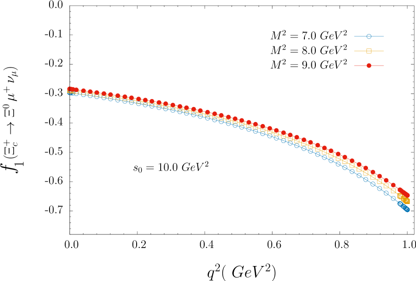
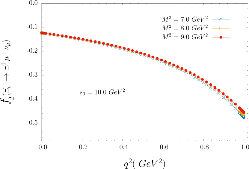
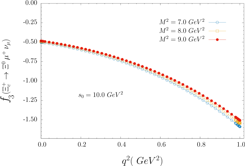
Figure 1: The dependency of the form factors $f_{1}$, $f_{2}$, and $f_{3}$ for the $\Xi_{c}^{+}\rightarrow\Xi^{0}\,\mu^{+}\,\nu_{\mu}$ transition on $q^{2}$, at $s_{0}=10~{}GeV^{2}$, and several values of the Borel mass parameter $M^{2}$

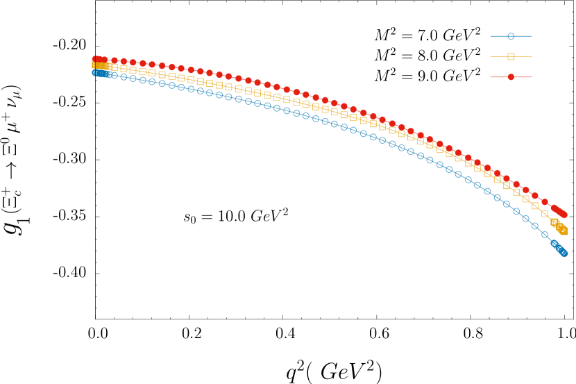
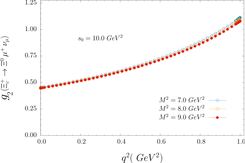
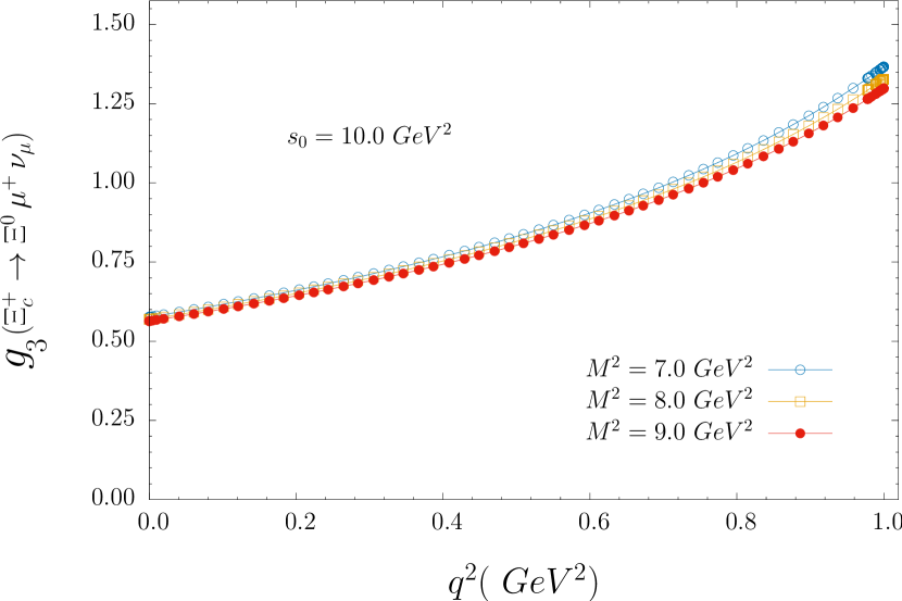
Figure 2: The dependency of the form factors $g_{1}$, $g_{2}$, and $g_{3}$ for the $\Xi_{c}^{+}\rightarrow\Xi^{0}\,\mu^{+}\,\nu_{\mu}$ transition on $q^{2}$, at $s_{0}=10~{}GeV^{2}$, and several values of the Borel mass parameter $M^{2}$

Having obtained the results for the form factors, we estimate the decay widths of the $\Xi_{c}\to B\ell\nu$ decays. The width of these decays can be calculated using helicity formalism Gutsche et al. (2015). We choose the rest frame of $\Xi_{c}$ baryon, where the z-axis points along the $W_{off-shell}$ to calculate the helicity amplitudes, and we obtain

$$H_{+{1\over 2},+1}^{V(A)} = \sqrt{2Q_{\mp}}\left[f_{1}(g_{1})-{m_{\pm}\over m_{{}_{\Xi_{c}}}}f_{2}(g_{2})\right]~{},$$

$$H_{+{1\over 2},0}^{V(A)} = {\sqrt{Q_{\mp}}\over\sqrt{q^{2}}}\left[m_{\pm}f_{1}(g_{1})-{q^{2}\over m_{{}_{\Xi_{c}}}}f_{2}(g_{2})\right]~{},$$

$$H_{+{1\over 2},t}^{V(A)} = {\sqrt{Q_{\pm}}\over\sqrt{q^{2}}}\left[m_{\mp}f_{1}(g_{1})-{q^{2}\over m_{{}_{\Xi_{c}}}}f_{3}(g_{3})\right]~{},$$

where $m_{\pm}=m_{{}_{\Xi_{c}}}\pm m_{B}$, and $Q_{\pm}=m_{\pm}^{2}-q^{2}$.

In these expressions, the first and second subindices describe the helicities of the $B$ baryon and virtual $W$, correspondingly. The amplitudes for the negative values of the helicities can be obtained from the parity consideration, i.e.,

$$H_{-\lambda_{B},-\lambda_{W}}^{V} = H_{\lambda_{B},\lambda_{W}}^{V}~{},$$

$$H_{-\lambda_{B},-\lambda_{W}}^{A} = -H_{\lambda_{B},\lambda_{W}}^{A}~{},$$

The total helicity amplitude is given by,

$$H_{\lambda_{B},\lambda_{W}}=H_{\lambda_{B},\lambda_{W}}^{V}-H_{\lambda_{B},\lambda_{W}}^{A}~{}.$$

Using the expressions of above-given helicity amplitudes for the differential decay widths, we obtain

$${d\Gamma(\Xi_{c}\to B\ell\nu)\over dq^{2}} = {G_{F}^{2}\over(2\pi)^{3}}\left|V_{cq}\right|^{2}{\sqrt{\lambda(m_{{}_{\Xi_{c}}}^{2},m_{B}^{2},q^{2})}(q^{2}-m_{\ell}^{2})^{2}\over 48m_{{}_{\Xi_{c}}}^{3}q^{2}}\Bigg{\{}\left|H_{+{1\over 2},+1}\right|^{2}+\left|H_{{-{1\over 2}},-1}\right|^{2}$$

$$+ \left(1+{m_{\ell}^{2}\over 2q^{2}}\right)\left(\left|H_{+{1\over 2},0}\right|^{2}+\left|H_{-{1\over 2},0}\right|^{2}\right)+{3m_{\ell}^{2}\over q^{2}}\left(\left|H_{+{1\over 2},t}\right|^{2}+\left|H_{{-{1\over 2}},t}\right|^{2}\right)\Bigg{\}}~{},$$

where $G_{F}$ is the Fermi constant, $V_{cq}$ is the CKM matrix element $(q=s~{}{\rm or}~{}d)$, and

$$\lambda(m_{{}_{\Xi_{c}}}^{2},m_{B}^{2},q^{2})=m_{{}_{\Xi_{c}}}^{4}+m_{B}^{4}+q^{4}-2m^{2}_{{\Xi_{c}}}m_{B}^{2}-2m_{{}_{\Xi_{c}}}^{2}q^{2}-2m_{B}^{2}q^{2}~{},$$

The differential decay width for the $\Xi_{c}^{\ast}\to B\ell\nu$ decay can be obtained from $\Xi_{c}\to B\ell\nu$ decay by making the following replacements, $f_{1}\to-\widetilde{g}_{1},~{}f_{2}\to\widetilde{g}_{2},~{}g_{1}\to-\widetilde{f}_{1},~{}g_{2}\to\widetilde{f}_{2}$, and $m_{{}_{\Xi_{c}}}\to m_{{}_{\Xi_{c}^{\ast}}}$.

Using the values of the CKM matrix elements $\left|V_{cd}\right|=0.2211\pm 0.0700$ and $\left|V_{cs}\right|=0.987\pm 0.011$ Zyla et al. (2020) and the $\Xi_{c}$ life time $\tau(\Xi_{c}^{0})=(1.53\pm 0.06)\times 10^{-13}~{}s$, and $\tau(\Xi_{c}^{+})=(4.56\pm 0.05)\times 10^{-13}~{}s$ we can predict the branching ratios of the corresponding semileptonic decays. Our results are presented in Table 4. In this table, we also present the values of the branching ratios of the semileptonic $\Xi_{c}\to B\ell\nu$ decays obtained from other theoretical approaches, as well as the latest announced experimental results. From a comparison of the predictions of the different approaches, we see that our results are close to that of the ones given in Ke et al. (2021) as well as the experimental measurements Li et al. (2021); Acharya et al. (2021). On the other hand, the obtained branching ratios are slightly smaller than the results presented in Geng et al. (2019); Faustov and Galkin (2019); Zhang et al. (2021) but larger than the values obtained in Zhao (2021, 2018). However, our results are considerably different for the results obtained in Azizi et al. (2012) for the $\Xi_{c}\to\Xi\ell\nu$ decay, although they applied the same method as used in this work. This discrepancy can be explained as follows. The interpolating current of $\Xi_{c}$ baryon interacts not only with ground state positive parity baryons $J^{P}=(\frac{1}{2})^{+}$ but also with $J^{P}=\frac{1}{2}^{-}$ negative parity baryon which was neglected in Azizi et al. (2012). Thus, the dispersion relation of $\Xi_{c}$ baryon is modified, and since the mass difference between these states is around 300 MeV, the results change considerably.

Decay Channel	Present Work	BELLE Li et al. (2021)	ALICE Acharya et al. (2021)	SU(3) Geng et al. (2018)	SU(3) Geng et al. (2019)	RQM Faustov and Galkin (2019)	LATTICE Zhang et al. (2021)	3PSR Zhao (2021)	LCSR Azizi et al. (2012)	LFQM Zhao (2018)	LF Ke et al. (2021)
$\Xi_{c}^{0}\to\Xi^{-}e^{+}\nu_{e}$	$1.85\pm 0.56$	$1.72\pm 0.10\pm 0.12\pm 0.50$	$1.8\pm 0.2$	$4.87\pm 1.74$	$2.4\pm 0.3$	$2.38$	$2.38\pm 0.30\pm 0.33$	$1.45\pm 0.31$	$7.26\pm 2.54$	$1.354$	$1.72\pm 0.35$
$\Xi_{c}^{0}\to\Xi^{-}\mu^{+}\nu_{\mu}$	$1.79\pm 0.54$	$1.71\pm 0.17\pm 0.13\pm 0.50$	$1.8\pm 0.2$	$---$	$2.4\pm 0.3$	$2.31$	$2.29\pm 0.29\pm 0.31$	$1.45\pm 0.31$	$7.15\pm 2.50$	—
$\Xi_{c}^{+}\to\Xi^{0}e^{+}\nu_{e}$	$5.51\pm 1.65$	—	—	$3.38_{-2.26}^{+2.10}$	$9.8\pm 1.1$	$9.40$	$7.18\pm 0.90\pm 0.98$	—	$28.6\pm 10$	$5.39$	$5.2\pm 1.02$
$\Xi_{c}^{+}\to\Xi^{0}\mu^{+}\nu_{\mu}$	$5.34\pm 1.61$	—	—	—	$9.8\pm 1.1$	$9.11$	$6.91\pm 0.87\pm 0.93$	—	$28.2\pm 9.9$	—	—
$\Xi_{c}^{+}\to\Lambda^{0}e^{+}\nu_{e}$	$0.092\pm 0.028$	—	—	—	$0.166\pm 0.018$	$0.127$	—	—	—	$0.082$	—
$\Xi_{c}^{+}\to\Lambda^{0}\mu^{+}\nu_{\mu}$	$0.089\pm 0.027$	—	—	—	—	$0.124$	—	—	—	—

Table 4: The existing experimental and theoretical results on the branching ratios (in %) of the semileptonic $\Xi_{c}\rightarrow Bl\nu$ decays.

Our predictions on the branching ratios of $\Xi_{c}^{+}\to\Lambda\ell\nu_{\ell}$ are also quite in agreement with the results of Faustov and Galkin (2019) within the error. The predictions on the branching ratios can further be improved by more precise determination of the input parameters appearing in DAs of the $\Xi$ and $\Lambda$ baryons, as well as taking into account ${\cal O}(\alpha_{s})$ corrections.

IV Conclusion

The form factors of the semileptonic $\Xi_{c}\to\Xi(\Lambda)\ell\nu$ decays are studied in the framework of the light cone QCD sum rules method. In order to eliminate the contamination of the negative parity $\Xi_{c}^{\ast}$ baryon, the combination of the sum rules obtained from different Lorentz structures is used.

Using the obtained results on the form factors and applying the helicity formalism, we also estimated the corresponding branching ratios of the considered decays. Moreover, our results on the branching ratios are compared with the predictions of the other approaches as well as with the experimental measurements.

The branching ratios of $\Xi_{c}\to\Xi\ell\nu$ decays has already been studied in various models like Relativistic Quark Model Faustov and Galkin (2019), LATTICE QCD Zhang et al. (2021), 3-point sum rules Zhao (2021), Light Front Quark Models Zhao (2018); Ke et al. (2021). Our calculations within the light cone sum rule showed that the resutls are in good agreement with the experimental measurements done by BELLE Li et al. (2021) and ALICE Acharya et al. (2021) Collaborations.

The discrepancy between our finding and the results of Azizi et al. (2012) in which the same method was used can be explained by taking into account the contributions of the $\Xi_{c}^{\ast}$ baryon that was neglected in Azizi et al. (2012).

Moreover, we also estimated the decay width of the CKM suppressed semileptonic $\Xi\rightarrow\Lambda l\nu$ decay within the light-cone sum rules. The obtained branching ratios are close the predictions of Faustov and Galkin (2019) and the magnitude of the obtained value shows that it has potential to be measured in the future experiments

References

Li et al. (2021)Y. B. Li et al. (Belle), “Measurements of the branching fractions of
semileptonic decays and
asymmetry parameter of decay,” (2021), arXiv:2103.06496 [hep-ex] .
Acharya et al. (2021)Shreyasi Acharya et al. (ALICE), “Measurement of the cross
sections of and baryons and
branching-fraction ratio BR()/BR() in pp collisions at 13
TeV,” (2021), arXiv:2105.05187 [nucl-ex] .