Scalar and Tensor Perturbations in DHOST Bounce Cosmology

Abstract

We investigate the bounce realization in the framework of DHOST cosmology, focusing on the relation with observables. We perform a detailed analysis of the scalar and tensor perturbations during the Ekpyrotic contraction phase, the bounce phase, and the fast-roll expansion phase, calculating the power spectra, the spectral indices and the tensor-to-scalar ratio. Furthermore, we study the initial conditions, incorporating perturbations generated by Ekpyrotic vacuum fluctuations, by matter vacuum fluctuations, and by thermal fluctuations. The scale invariance of the scalar power spectrum can be acquired introducing a matter contraction phase before the Ekpyrotic phase, or invoking a thermal gas as the source. The DHOST bounce scenario with cosmological perturbations generated by thermal fluctuations proves to be the most efficient one, and the corresponding predictions are in perfect agreement with observational bounds. Especially the tensor-to-scalar ratio is many orders of magnitude within the allowed region, since it is suppressed by the Hubble parameter at the beginning of the bounce phase.

1 Introduction

Bounce cosmology [1, 2, 3, 4, 5, 6] can serve as a very early universe scenario for the structure formation alternative to the standard inflationary cosmology (see e.g. [7] for critical reviews on inflation and its alternatives). Nonsingular bounce cosmology has the merit to avoid the initial singularity problem [8, 9] encountered by inflationary cosmology, which motivates the investigations on this field. However, bounce models also face new challenges such as the ghost and gradient instability problem [10, 13, 12, 11], the problem of anisotropic stress [14, 15, 16, 17] (also known as the Belinski–Khalatnikov–Lifshitz (BKL) instability [18]), and the tension between tensor-to-scalar ratio and non-Gaussianities [19, 20, 21, 22, 23, 24]. Nevertheless, it is important to discuss the validity of nonsingular bounce cosmology from the viewpoint of cosmological observations.

Many attempts have been made to evade the aforementioned problems in constructing a nonsingular bounce scenario [25, 26, 27]. In the literature, higher-order scalar-tensor theories beyond the Horndeski/Generalized Galileon theory are introduced to solve the gradient instability problem [28, 29, 30, 31, 33, 32, 34, 35, 36, 37], which occurs inevitably in bounce models constructed within second-order scalar-tensor theories [38, 39, 40]. Moreover, the Ekpyrotic scenario [41], during which the energy density of the dominated matter fluid blue-shifts faster than the anisotropic stress, can prevent the development of the BKL instability. Additionally, the tension between tensor-to-scalar ratio and non-Gaussianities predicted by matter bounce cosmology can be evaded by generalizing the action of the matter component [24]. As a next step after addressing the conceptual issues of nonsingular bounce models, it is important to study their observational quantities, such as the amplitude and the spectral index of primordial curvature perturbations, as well as the associated tensor-to-scalar ration, so that these models can be testable in observations, and confront the predictions with observational data.

In this work we focus on one class of nonsingular bounce cosmology, namely the DHOST bounce developed in [42] in the framework of Degenerate Higher-Order Scalar-Tensor (DHOST) theories. The DHOST bounce models are shown to be free from ghost, gradient and BKL instabilities, and thus they provide a solid realization of a healthy nonsingular bounce scenario. It is then natural to ask whether such models can survive from the observational confrontation. We shall study the scalar and tensor power spectra within the simplest case, namely the DHOST bounce scenario with a single bounce phase.

The manuscript is organized as follows. In Section 2 we briefly review the basics of DHOST bounce, and describe the specific model that shall be analyzed. Then we investigate the background dynamics and provide its parametrization in Section 3. The dynamics of cosmological perturbation is investigated in Section 4, and the power spectra with different initial conditions are calculated in Section 5. Finally, we conclude with relevant discussions in Section 6.

Throughout the work we consider the signature of the metric as $(+,-,-,-)$, and we denote the reduced Planck mass by $M_{p}\equiv 1/\sqrt{8\pi G}=1$, where $G$ is the Newton’s gravitational constant, and all used parametric values are in Planck units. The dot symbol represents differentiation with respect to the cosmic time $t$: $\dot{\phi}\equiv d\phi/dt$, and a comma in the subscript denotes partial derivative: $\phi_{,\mu}\equiv\partial_{\mu}\phi$. We define $X\equiv\frac{1}{2}\nabla_{\mu}\phi\nabla^{\mu}\phi$ to be the canonical kinetic term of the scalar field. The subscript “B-” and “B+” labels the start/end of the bounce phase (e.g. $t_{B-}$ represents the cosmic time at the beginning of the bounce phase). Additionally, at the bounce point we normalize the scale factor as $a_{B}=1$ and the cosmic time as $t_{B}=0$, while the conformal time, defined as $\tau\equiv\int dt/a$, is also set to 0 at the bounce point $\tau_{B}=0$. Furthermore, we use the subscripts $f_{X}$ and $f_{\phi}$ to denote $f_{X}\equiv\partial f/\partial X$ and $f_{\phi}\equiv\partial f/\partial\phi$, respectively. Lastly, we focus on a flat Friedmann-Robertson-Walker (FRW) geometry with metric

$$ds^{2}=dt^{2}-a^{2}(t)\,\delta_{ij}dx^{i}dx^{j},$$ (1.1)

with $a(t)$ the scale factor.

2 The basics of DHOST Bounce

In this section, we briefly review the DHOST bounce scenario developed in [42].

2.1 The Generic Action

The generic action is taken to be

$$S=\int d^{4}x\sqrt{-g}\Big{[} -{M_{p}^{2}}[1+f(\phi,X)]\frac{R}{2}+K(\phi,X)+Q(\phi,X)\Box\phi$$

$$-\frac{f}{4X}\left(L_{1}^{(2)}-L_{2}^{(2)}\right)+\frac{f-2Xf_{X}}{4X^{2}}\left(L_{4}^{(2)}-L_{3}^{(2)}\right)\Big{]}~{},$$ (2.1)

where $R$ represents the Ricci scalar (thus the term $-R/2$ corresponds to the standard Einstein-Hilbert action). Additionally, the term $K+Q\Box\phi$ is a part of the Galileon/Horndeski action [43, 44, 45, 46], which has been introduced to cosmology and analyzed in [47, 48, 49, 50, 51, 52, 53]. The function $f\equiv f(\phi,X)$ represents the DHOST coupling:

$$\mathcal{L}_{D}\equiv-M_{p}^{2}f(\phi,X)\frac{R}{2}-\frac{f}{4X}\left(L_{1}^{(2)}-L_{2}^{(2)}\right)+\frac{f-2Xf_{X}}{4X^{2}}\left(L_{4}^{(2)}-L_{3}^{(2)}\right)~{}.$$ (2.2)

We provide a brief introduction to the quadratic DHOST theory in Appendix A, and we show that the action (2.1) belongs to the ${}^{(2)}N-I$ type DHOST theory , thus the model is free from the Ostrogradsky instabilities [54] which plagues most of higher-order scalar-tensor theories.

2.2 Realization of DHOST Bounce with a Single Bounce

In the above construction, different choices of $f(\phi,X)$ will lead to different cosmological bouncing scenarios. In [42] two specific cases were discussed. If $f\equiv f(X)$, the DHOST coupling will not affect the background dynamics, and the cosmological scenario will be similar to the previously developed ones [51] with a single bounce phase. On the other hand, if $f\equiv f(\phi)$ the bouncing scenario will be drastically changed, and there can exist multiple bounce [55] phases.

As stated in the Introduction, in this work we will focus on the simple case where $f\equiv f(X)$, and thus there exists only one bouncing phase, since the results are comparable to the previous work [51]. The spectra with multiple bouncing phase will be studied in a following project, and for interested readers we refer to the pioneer work [56] on this topic.

We consider the operators in action (2.1) to be

$$K(\phi,X)={M_{p}^{2}}[1-g(\phi)]X+\beta X^{2}-V(\phi)~{},~{}Q(\phi,X)=\gamma X~{},~{}f(\phi,X)={cX^{2}+\frac{d}{M_{p}^{2}}X^{3}}~{},$$ (2.3)

where the functions $g(\phi)$ and $V(\phi)$ are defined as

$$g(\phi)=-\frac{2g_{0}}{e^{-\sqrt{\frac{2}{p}}\phi}+e^{b_{g}\sqrt{\frac{2}{p}}\phi}}~{},~{}V(\phi)=-\frac{2V_{0}}{e^{-\sqrt{\frac{2}{q}}\phi}+e^{b_{V}\sqrt{\frac{2}{q}}\phi}}~{},$$ (2.4)

with $g_{0}$, $p$, $b_{g}$, $V_{0}$, $q$, $b_{V}$, $\beta$, $\gamma$, $c$, $d$ the model parameters. We follow the convention of [51] and we consider $\phi$ to be dimensionless, which implies that all parameters are dimensionless, except for $V_{0}$ has dimension $[M]^{4}$.

In the following sections we will use the parameter values

$$V_{0}=10^{-8}~{},~{}g_{0}=1.1~{},~{}\beta=5~{},~{}\gamma=3\times 10^{-3}~{},$$

$$b_{V}=100~{},~{}b_{g}=0.5~{},~{}p=0.01~{},~{}q=\frac{6}{31}~{},$$ (2.5)

and DHOST function $f(X)=450X^{2}+500000X^{3}$ (all dimension-full parameters are measured in Planck units) to numerically verify the approximations of the analytic calculation. Particularly, in Section 5, we calculate the observable parameters (scalar amplitude $A_{s}$, scalar spectra index $n_{s}$ and tensor-to-scalar ratio $r$) and show that the predicted values are compatible with Cosmic Microwave Background (CMB) data with the model parameters being (2.2) (see (5.19)).

Before proceeding, in order to provide a complete picture, in Fig. 1 we depict the dynamics of the Hubble parameter $H\equiv\frac{\dot{a}}{a}$ and the sound speed of scalar/tensor perturbations $c_{s}^{2}$ and $c_{T}^{2}$ [42]. The bounce phase takes place in the neighborhood of $t=0$, where the Hubble parameter changes from negative to positive. Moreover, $c_{s}^{2}$ and $c_{T}^{2}$ are positive during the whole cosmological process, which illustrate that the model under consideration is free from the gradient instability. In the following we perform the detailed analysis, explanation, and calculation of observables.

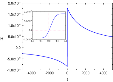
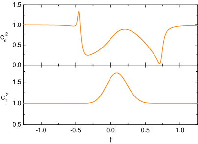
Figure 1: Evolution of the Hubble parameter $H$ (left) and the sound speeds of scalar and tensor perturbations, $c_{s}^{2}$ and $c_{T}^{2}$ respectively (right). The background parameters are chosen as in (2.2). Both $c_{s}^{2}$ and $c_{T}^{2}$ exhibit superluminal behavior near the bounce point, which is a common feature in theories beyond Horndeski [57, 58]

.

3 Background

The background equations of motion for the model at hand are [42]

$$3H^{2}=\rho\equiv\frac{1}{2}\left[1-g(\phi)\right]\dot{\phi^{2}}+\frac{3}{4}\beta\dot{\phi}^{4}+3\gamma H\dot{\phi}^{3}+V(\phi)~{},$$ (3.1)

$$-2\dot{H}-3H^{2}=P\equiv\frac{1}{2}\left[1-g(\phi)\right]\dot{\phi^{2}}+\frac{3}{4}\beta\dot{\phi}^{4}-\gamma\dot{\phi}^{2}\ddot{\phi}-V(\phi)~{},$$ (3.2)

where $\rho$ and $P$ are the energy density and pressure of the scalar field. Conventionally, one may define the equation of state (EoS) parameter as $w\equiv P/\rho$. Note that the DHOST coupling $f(X)$ is absent from the equations (3.1) and (3.2), hence the background evolution is the same as in the Horndeski/Galileon bounce proposed in [51]. Therefore, the whole cosmological evolution can be separated into three phases: the Ekpyrotic phase where the universe undergoes a contraction phase, the nonsingular bounce phase where the universe transits from contraction to expansion, and the fast-roll expansion phase which finally connects with the standard Big Bang cosmology. We can then follow the parametrization from [51], as described below. The numerical results for the evolution of the Hubble parameter are shown in Fig. 1.

3.1 Ekpyrotic Contraction Phase

This phase begins at the far past where $\phi\ll-1$, and ends when the function $g(\phi)$ reaches the critical value $1$. In this phase, when $g(\phi)$ tends to $0$, the Lagrangian approaches the canonical form: $\mathcal{L}\to 1/2\partial_{\mu}\phi\partial^{\mu}\phi-V(\phi)$. Accordingly, it admits the Ekpyrotic attractor solution

$$\phi\simeq-\sqrt{\frac{q}{2}}\ln\left[\frac{2V_{0}t^{2}}{q(1-3q)}\right]~{},$$ (3.3)

with $q$ a parameter related to the nearly constant EoS parameter during this phase, $w_{c}$, as $w_{c}\simeq-1+\frac{2}{3q}$. We mention that in order to make the model free from the BKL instability [18], which plagues many bouncing scenarios [14, 15], the energy density of $\phi$ should increase faster than the anisotropic stress, which indicates the constraint $0<q<1/3$.

Since during Ekpyrotic contraction the EoS parameter $w_{c}$ is approximately constant, the scale factor $a(\tau)$ evolves accordingly as

$$a(\tau)=a_{B-}\left(\frac{\tau_{-}-\tau}{\tau_{-}-\tau_{B-}}\right)^{\frac{q}{1-q}}~{},\mathcal{H}\simeq\frac{-q}{(1-q)(\tau_{-}-\tau)}~{},$$ (3.4)

where $\tau_{-}$ and $a_{B-}$ are proper integration constants and $\mathcal{H}\equiv\partial_{\tau}a/a$ is the conformal Hubble parameter. The boundary condition, i.e. $g(\phi)$ reaches $1$ at the end of Ekpyrotic contraction $\tau=\tau_{B-}$, gives

$$\tau_{-}=\tau_{B-}-\frac{q}{(1-q)\mathcal{H}_{B-}}~{}.$$ (3.5)

Finally, we comment that in the Ekpyrotic phase, there exists only one scalar field $\phi$ whose EoS parameter satisfies $w_{c}>1$, thus the principle of finite amplitude developed in [59] is not violated in our model.

3.2 Bounce Phase

As we have mentioned, we normalize the time axis by setting $t=0$ at the bounce point, i.e $H(0)=0$, while the scale factor is normalized as $a(0)=1$. Then, as it has been shown in [60, 61, 62, 63], the evolution of the Hubble parameter near the bounce point can be well approximated by a linear function of cosmic time $H\simeq\Gamma t$. The parametrization is valid in a class of fast bounce models, and the magnitude of $\Gamma$ is usually set by the detailed microphysics of the bounce.

In the specific parametric choice of (2.2), $\Gamma$ is of the order of $\mathcal{O}(10^{-4})$, and the beginning/ending time of bounce phase, namely $t_{B-}$ and $t_{B+}$, is of the order of $\mathcal{O}(1)$. Thus, the conformal time $\tau$ is

$$\tau=\int_{0}^{t}\frac{dt^{\prime}}{a(t^{\prime})}=\int_{0}^{t}e^{-\frac{1}{2}\Gamma t^{\prime 2}}dt^{\prime}\simeq t-\frac{1}{6}\Gamma t^{3}+\mathcal{O}(t^{5})\simeq t~{}.$$ (3.6)

This implies that in the bounce phase the cosmic time $t$ and the conformal time $\tau$ are almost equivalent. This is not surprising: a fast bounce means that the scale factor will not change significantly during the bounce phase, therefore the difference between conformal and cosmic time will be minor.

The dynamics of the scale factor and the scalar field is then

$$H\simeq\Gamma t~{},~{}a(t)\simeq e^{\frac{1}{2}\Gamma t^{2}}~{},~{}\dot{\phi}\simeq\dot{\phi}_{B}\exp{\left(-\frac{t^{2}}{T^{2}}\right)}~{},$$ (3.7)

while in terms of the conformal time

$$~{}\mathcal{H}\simeq\Gamma\tau~{},~{}a(\tau)\simeq e^{\frac{1}{2}\Gamma\tau^{2}}~{}.$$ (3.8)

Here, $\dot{\phi}_{B}$ denotes the value of the derivative of the scalar field $\phi$ at the bouncing point $t=0$, which is $\dot{\phi}_{B}^{2}\simeq 2(g_{0}-1)/3\beta$, while the parameter $T$ is approximately one quarter of the duration of the bounce.

3.3 Fast-roll Expansion

After the bounce, the $\dot{\phi}^{2}$ term decreases and thus the scalar field $\phi$ will cross the critical value where the function $g(\phi)$ decreases to $1$, and the scalar field abandons the ghost condensate state. Then the Lagrangian of $\phi$ acquires the canonical form with a relatively flat potential, and thus the scalar field will enter a fast-roll state with EoS parameter $w\simeq 1$. Hence, the scale factor will behave as $a\propto t^{1/3}$. In particular, we have

$$a(t)=a_{B+}\left(\frac{t-t_{+}}{t_{B+}-t_{+}}\right)^{1/3}~{},~{}H(t)=\frac{1}{3(t-t_{+})}~{},$$ (3.9)

which gives the conformal time $\tau$ as

$$\left(\frac{\tau-\tau_{+}}{\tau_{B+}-\tau_{+}}\right)=\left(\frac{t-t_{+}}{t_{B+}-t_{+}}\right)^{\frac{2}{3}}~{},$$ (3.10)

where $\tau_{+}$ and $t_{+}$ are integration constants.

In terms of the conformal time $\tau$, the background evolution can be expressed as

$$a(\tau)=a_{B+}\left(\frac{\tau-\tau_{+}}{\tau_{B+}-\tau_{+}}\right)^{\frac{1}{2}}~{},~{}H(\tau)=\frac{1}{3(t_{B+}-t_{+})}\left(\frac{\tau-\tau_{+}}{\tau_{B+}-\tau_{+}}\right)^{-\frac{3}{2}}~{},$$ (3.11)

which gives the conformal Hubble parameter as

$$\mathcal{H}(\tau)=a(\tau)H(\tau)=\frac{1}{2(\tau-\tau_{+})}~{}.$$ (3.12)

3.4 Matching Conditions at the Background Level

The scale factor $a$, the Hubble parameter $H$, the scalar field $\phi$ and its first derivative $\dot{\phi}$, should be continuous at the transition surfaces $\tau=\tau_{B-}$ and $\tau=\tau_{B+}$. In this section, we explicitly elaborate the constraints that are required when incorporating the cosmological perturbations.

However, we mention that, as we will see in the next section, $\phi$ and $\dot{\phi}$ will not affect the dynamics of cosmological perturbations in both the contraction and expansion phases. Hence, there is no need to impose the continuity condition on the scalar-field content. The same argument applies to the scale factor $a$ at the end of Ekpyrotic contracting phase. Therefore, the remaining tasks are to determine the condition for the continuity of $H$ at $\tau=\tau_{B+}$, $\tau=\tau_{B-}$, and the continuity of $a$ at $\tau=\tau_{B+}$.

At the transition surface $\tau=\tau_{B-}$, the continuity of conformal Hubble parameter $\mathcal{H}$ gives

$$\mathcal{H}_{B-}\equiv\mathcal{H}(\tau=\tau_{B-})=\Gamma\tau_{B-}~{},$$ (3.13)

which can be used to determine the value of $\tau_{-}$ from equation (3.5). Similarly, at the transition surface $\tau=\tau_{B+}$, the continuity of $a$ and $\mathcal{H}$ gives

$$a_{B+}\equiv a(\tau_{B+})=e^{\frac{1}{2}\Gamma\tau_{B+}^{2}}~{},~{}\ \ \ \ \mathcal{H}(\tau_{B+})=\frac{a_{B+}}{3(t_{B+}-t_{+})}=\Gamma\tau_{B+}~{},$$ (3.14)

along with the approximation $\tau_{B+}\simeq t_{B+}$ from the bounce phase, where the integration constant $t_{+}$ is determined by

$${t_{+}=t_{B+}-\frac{a_{B+}}{3\Gamma\tau_{B+}}}~{}.$$ (3.15)

4 Evolution of Perturbations

In this section, we proceed to the detailed investigation of the scalar and tensor perturbations. Similar to the previous section, after providing the perturbation equations, we will perform the analysis for the various phases separately.

4.1 Perturbations Equations

The actions for the scalar and tensor perturbations at linear level are [42, 64, 65]

$$S_{2,S}=\int d\tau d^{3}x\frac{z_{s}^{2}}{2}\left[\zeta^{\prime 2}-c_{s}^{2}(\partial_{i}\zeta)^{2}\right]~{},$$ (4.1)

$$S_{2,T}\equiv\int d\tau d^{3}x\frac{z_{T}^{2}}{2}\left[\gamma_{ij}^{\prime 2}-c_{T}^{2}(\nabla_{k}\gamma_{ij})^{2}\right]~{},$$ (4.2)

where

$$\frac{z_{s}^{2}}{2a^{2}}=3+\frac{2\left[\dot{\phi}^{2}K_{X}+\dot{\phi}^{4}K_{XX}-6H^{2}+12\gamma H\dot{\phi}^{3}\right]}{(\gamma\dot{\phi}^{3}-2H)^{2}}~{},$$ (4.3)

$$\left(-\frac{z_{s}^{2}}{2a^{2}}\right)c_{s}^{2}=1+f+\frac{2}{a}\frac{d}{dt}\left[\frac{a(f_{X}\dot{\phi}^{2}-f-1)}{2H-\gamma\dot{\phi}^{3}}\right]~{},$$ (4.4)

$$z_{T}^{2}=\frac{1}{4}a^{2}~{},~{}c_{T}^{2}=1+f~{}.$$ (4.5)

Varying (4.1) with respect to $\zeta$ leads to the Mukhanov-Sasaki (MS) equation [66, 67, 68] for scalar perturbations, namely

$$v_{k}^{\prime\prime}+\left(c_{s}^{2}k^{2}-\frac{z_{s}^{\prime\prime}}{z_{s}}\right)v_{k}=0~{},$$ (4.6)

where $v_{k}\equiv z_{s}\zeta_{k}$ is the MS variable. On the other hand, the tensor perturbations contain two modes. As usual we decompose the tensor perturbations $\gamma_{ij}$ as

$$\gamma_{ij}(\tau,\vec{x})=\gamma_{+}(\tau,\vec{x})e_{ij}^{+}+\gamma_{\times}(\tau,\vec{x})e_{ij}^{\times}~{},$$ (4.7)

with two fixed polarization tensors, $e_{ij}^{+}$ and $e_{ij}^{\times}$. Hence, the action for tensor perturbation is canonical and leads to the standard MS equation:

$$\mu_{k}^{\prime\prime}+\left(c_{T}^{2}k^{2}-\frac{a^{\prime\prime}}{a}\right)\mu_{k}=0~{},$$ (4.8)

with $\mu_{k}\equiv\frac{1}{2}a\gamma_{k}$ the MS variable.

4.2 Evolution of Perturbations in Ekpyrotic Contraction Phase

In the Ekpyrotic contracting phase we have $|\phi|\gg 1$ and $\dot{\phi}\ll 1$, therefore $g\simeq 0$ and the higher order operators are suppressed. As analyzed in [51], we have

$$z_{s}^{2}\simeq a^{2}/q~{},~{}c_{s}^{2}\simeq 1~{},~{}c_{T}^{2}\simeq 1~{}.$$ (4.9)

The validity of (4.9) is also verified numerically in [42].

Using equation (3.4) and (4.9) we obtain

$$\frac{z_{s}^{\prime\prime}}{z_{s}}=\frac{a^{\prime\prime}}{a}=\frac{q(2q-1)}{(1-q)^{2}(\tau-\tau_{-})^{2}}~{},$$ (4.10)

hence the MS equations for scalar (4.6) and tensor perturbations (4.8) become

$$v_{k}^{\prime\prime}+\left[k^{2}-\frac{q(2q-1)}{(1-q)^{2}(\tau-\tau_{-})^{2}}\right]v_{k}=0~{},$$ (4.11)

and

$$\mu_{k}^{\prime\prime}+\left[k^{2}-\frac{q(2q-1)}{(1-q)^{2}(\tau-\tau_{-})^{2}}\right]\mu_{k}=0~{}.$$ (4.12)

Let us first investigate the scalar perturbations. The general analytical solution of (4.11) is

$$v_{k}^{c}(\tau)=b_{s,1}(k)\sqrt{\tau_{-}-\tau}J_{\nu_{c}}[k(\tau_{-}-\tau)]+b_{s,2}(k)\sqrt{\tau_{-}-\tau}Y_{\nu_{c}}[k(\tau_{-}-\tau)]~{},$$ (4.13)

with

$$\nu_{c}=\frac{1-3q}{2(1-q)}=\frac{1}{2}-\frac{q}{1-q}~{}.$$ (4.14)

Here, $J$ and $Y$ are Bessel functions, and we introduce the superscript “c” in $v_{k}^{c}$ to denote the contraction phase. Recalling that, for small arguments, the Bessel function has the asymptotic behavior

$$J_{a}(x)\propto\left(\frac{x}{2}\right)^{a}~{},~{}Y_{a}(x)\propto\left(\frac{2}{x}\right)^{a}~{},0<x\ll\sqrt{a+1}~{},$$ (4.15)

we deduce that the first part in the expression of $v_{k}^{c}$ (4.13) will be suppressed in the contraction phase. Hence, at the end of the Ekpyrotic contraction phase, the dominant contribution to $v_{k}$ comes from the second mode in (4.13), and therefore we may set $b_{s,1}\simeq 0$ at that time.

Concerning the tensor perturbations, a similar analysis provides the general analytical solution as

$$\mu_{k}^{c}(\tau)=b_{t,1}(k)\sqrt{\tau_{-}-\tau}J_{\nu_{c}}[k(\tau_{-}-\tau)]+b_{t,2}(k)\sqrt{\tau_{-}-\tau}Y_{\nu_{c}}[k(\tau_{-}-\tau)]~{},$$ (4.16)

and thus its second mode will dominate at the end of Ekpyrotic contraction phase.

4.3 Evolution of Perturbations in Bounce Phase

In the bounce phase, the parametrization (3.7) gives (for the details see [51]):

$$\frac{z^{\prime\prime}}{z}\simeq\Gamma+\frac{2}{T^{2}}+\left(2\Gamma^{2}+\frac{6\Gamma}{T^{2}}+\frac{4}{T^{4}}\right)t^{2}~{},\frac{a^{\prime\prime}}{a}\simeq\Gamma(\Gamma\tau^{2}+1)~{}.$$ (4.17)

Recalling that $\Gamma$ is of the order of $\mathcal{O}(10^{-4})$ and $T\simeq 0.5$, we can approximately ignore the terms in (4.17) which contain $\Gamma$. Thus, the MS equations simplify to

$$v_{k}^{\prime\prime}-\left(\frac{2}{T^{2}}+\frac{4\tau^{2}}{T^{4}}-c_{s}^{2}k^{2}\right)v_{k}=0~{},$$ (4.18)

$$\mu_{k}^{\prime\prime}+\left(c_{T}^{2}k^{2}-\Gamma\right)\mu_{k}=0~{}.$$ (4.19)

Note that in (4.18) we have used the approximation $\tau\simeq t$. The scale-dependent terms, $c_{s}^{2}k^{2}$ in equation 4.18 and $c_{T}^{2}$ in equation 4.19, will be sub-dominant due to the smallness of the observable wavenumber $k$. Then, we can further neglect the $c_{T}^{2}k^{2}$ term in equation 4.19; however, we will maintain the $c_{s}^{2}k^{2}$ term in equation 4.18 to examine whether it could explain the deviation of scalar spectra index $n_{s}$ from $1$, deduced from CMB data.

The final general solution for tensor perturbations is

$$\mu_{k}=b_{t,3}e^{\sqrt{\Gamma}\tau}+b_{t,4}e^{-\sqrt{\Gamma}\tau}~{}.$$ (4.20)

However, $\sqrt{\Gamma}\tau_{B-}$ and $\sqrt{\Gamma}\tau_{B+}$ are of the order of $10^{-2}$, therefore the exponential function in (4.20) will be very close to $1$, which implies that the tensor perturbations will remain almost invariant during the bounce phase.

The general solution for scalar perturbations is the parabolic cylinder function. We provide the detailed analysis in Appendix B, and here we present the result. In particular, the dynamics of scalar perturbations can be approximated by the following semi-analytical solution:

$$v_{k}^{b}(\tau)\simeq b_{s,3}(k)e^{\int\omega_{k}(\tau)d\tau}+b_{s,4}(k)e^{-\int\omega_{k}(\tau)d\tau}~{},$$ (4.21)

$$\omega_{k}^{2}(\tau)=\frac{4\tau^{2}}{T^{4}}+\frac{2}{T^{2}}-c_{s}^{2}(\tau)k^{2}~{},$$ (4.22)

where $b_{s,3}$ and $b_{s,4}$ can be determined by the matching condition. It would also be useful to define the quantity

$$W_{k}(\tau)\equiv\int_{\tau_{B-}}^{\tau}\omega_{k}(x)dx~{},$$ (4.23)

with

$$\mathcal{F}_{s}(k)\equiv W_{k}(\tau_{B+})~{},$$ (4.24)

and since $\mathcal{F}_{s}\simeq 6\times 10^{4}$ is much larger than unity, the bounce phase will amplify the $b_{s,3}$ mode while it will suppress the $b_{s,4}$ mode. Hence, we can ignore the $b_{s,4}$ term in equation (4.21) at the end of the bounce phase. Besides, the $c_{s}^{2}(\tau)k^{2}$ term is sub-dominant in the expression of $\omega_{k}$, therefore the amplification factor $\mathcal{F}_{s}(k)$ is almost scale-independent, and the scalar spectra index will receive only a minor correction during the bounce phase.

From the above argument we can deduce that the tensor perturbations are almost invariant during the bounce phase, while the scalar perturbations get amplified by a nearly scale-independent factor $\mathcal{F}_{s}$. Hence, the existence of the bounce phase significantly suppresses the tensor-to-scalar ratio. As we will see in the following, this completely solves the problem of large tensor-to-scalar ratio of the usual matter bounce scenarios [62, 69, 22, 70].

4.4 Evolution of Perturbations in Fast-roll Expansion Phase

After the bounce, the scalar field returns to the canonical form, and behaves like a perfect fluid with EoS parameter $w=1$. As analyzed in [51], one has

$$z_{s}^{2}\propto a^{2}~{},~{}c_{s}^{2}\simeq 1~{},~{}c_{T}^{2}\simeq 1~{}.$$ (4.25)

Similarly, with the help of (3.9), we obtain

$$\frac{z_{s}^{\prime\prime}}{z_{s}}=\frac{a^{\prime\prime}}{a}=-\frac{1}{4}\left(\frac{1}{\tau-\tau_{+}}\right)^{2}~{},$$ (4.26)

and thus the MS equations (4.6) and (4.8) become

$$v_{k}^{\prime\prime}+\left[k^{2}+\frac{1}{4}\frac{1}{(\tau-\tau_{+})^{2}}\right]v_{k}=0~{},$$ (4.27)

$$\mu_{k}^{\prime\prime}+\left[k^{2}+\frac{1}{4}\frac{1}{(\tau-\tau_{+})^{2}}\right]\mu_{k}=0~{}.$$ (4.28)

The general solution for the perturbations is then

$$v_{k}^{e}(\tau)=b_{s,5}\sqrt{\tau-\tau_{+}}J_{\nu_{e}}[k(\tau-\tau_{+})]+b_{s,6}\sqrt{\tau-\tau_{+}}Y_{\nu_{e}}[k(\tau-\tau_{+})]~{},$$ (4.29)

$$\mu_{k}^{e}(\tau)=b_{t,5}\sqrt{\tau-\tau_{+}}J_{\nu_{e}}[k(\tau-\tau_{+})]+b_{t,6}\sqrt{\tau-\tau_{+}}Y_{\nu_{e}}[k(\tau-\tau_{+})]~{},$$ (4.30)

with $\nu_{e}=0$  .

4.5 Matching Conditions and Power Spectra

After obtaining general solutions to the perturbation equations in the various phases of the cosmological evolution, we now determine how the solutions should be matched at the transition surfaces $\tau=\tau_{B-}$ and $\tau=\tau_{B+}$. It was argued in [51] that the matching condition for scalar perturbations, deduced from [71, 72] (see also related discussions in [73, 74, 75, 76, 77]), is the continuity of $v$ and $v^{\prime}$ at the transition surface. The same argument can be applied to tensor perturbations (as we show in Appendix D), and $\mu$, $\mu^{\prime}$ are also continuous across the transition surface.

For scalar perturbations, the coefficients of (4.29) are

$$b_{s,5}=\frac{\mathcal{F}_{s}\Gamma\left(\nu_{c}\right)\left(1-2\nu_{c}\right)^{\frac{1}{2}-\nu_{c}}}{4^{1-\nu_{c}}\pi}\left(\frac{-\mathcal{H}_{B-}}{k}\right)^{\nu_{c}}\frac{w_{k+}}{\sqrt{-\mathcal{H}_{B-}\mathcal{H}_{B+}}}\ln\frac{ke^{\gamma_{E}}}{4\mathcal{H}_{B+}}b_{s,2}~{},$$ (4.31)

$$b_{s,6}=-\frac{\mathcal{F}_{s}\Gamma(\nu_{c})(1-2\nu_{c})^{\frac{1}{2}-\nu_{c}}}{2^{3-2\nu_{c}}}\left(\frac{-\mathcal{H_{B-}}}{k}\right)^{\nu_{c}}\frac{\omega_{k+}}{\sqrt{-\mathcal{H_{B-}}\mathcal{H_{B+}}}}b_{s,2}~{},$$ (4.32)

where the involved calculation details are presented in Appendix C. Here $\Gamma(x)$ is the gamma function and $\gamma_{E}\simeq 0.58$ is the Euler-Masheroni constant. The expression of $v_{k}^{e}$ as a function of the conformal Hubble parameter $\mathcal{H}$ is then

$$v_{k}^{e}(\mathcal{H})=\frac{\mathcal{F}_{s}\Gamma\left(\nu_{c}\right)\left(1-2\nu_{c}\right)^{\frac{1}{2}-\nu_{c}}}{4^{1-\nu_{c}}\pi\sqrt{2\mathcal{H}}}\left(\frac{-\mathcal{H_{B-}}}{k}\right)^{\nu_{c}}\left(\frac{\omega_{k+}\ln\frac{\mathcal{H}}{\mathcal{H}_{B+}}}{\sqrt{-\mathcal{H_{B-}}\mathcal{H_{B+}}}}-2\sqrt{\frac{\mathcal{H_{B+}}}{-\mathcal{H_{B-}}}}\right)b_{s,2}~{},$$ (4.33)

where we have used (3.12).

At the beginning of the fast-roll expansion phase, the wavenumber $k$ of observational interest lies outside the horizon since $k<\mathcal{H}_{B+}$. We will consider that the scalar perturbation is always outside the horizon during this phase. Standard cosmology implies that scalar perturbations should cross the horizon after the beginning of Big Bang Nucleosynthesis (BBN), hence the wavenumber observed by Large Scale Structure (LSS) must stay outside the horizon [78]. We can also see this by a simple estimation. If a certain mode $k$ crosses the horizon during the fast-roll expansion phase, then from $k=\mathcal{H}_{\star}$ and the formulae of subsection 3.3 we can acquire the corresponding energy density of the Universe $\rho_{\star}$ as

$$\rho_{\star}=3H_{\star}^{2}=3\left[\frac{(\tau_{B+}-\tau_{+})^{\frac{3}{2}}}{3(t_{B+}-t_{+})}\times(2\mathcal{H}_{\star})^{\frac{3}{2}}\right]^{2}=\frac{3k^{3}}{\mathcal{H}_{B+}}~{}.$$ (4.34)

The wavenumber $k$ of observational interest has an upper limit $k<10^{-10}$ in SI units. With the help of (4.34), the corresponding energy density is $\rho_{\star}\simeq\mathcal{O}(10^{-135})$ in Planck units, which is far below the energy scale of BBN. Hence, it is no possible for the scalar perturbations to cross the horizon during the fast-roll expansion phase.

Denoting the conformal Hubble parameter at the end of fast-roll expansion phase as $\mathcal{H}_{r}$, the definition of scalar power spectra

$$P_{\zeta}\equiv\frac{k^{3}}{2\pi^{2}}|\zeta_{k}|^{2}=\frac{k^{3}}{6\pi^{2}}|\frac{v_{k}^{e}}{a}|^{2}~{},$$ (4.35)

leads to (we use the approximation $a_{B+}\simeq 1$ and $a_{B-}\simeq 1$)

$$P_{\zeta}=\frac{\mathcal{F}_{s}^{2}\Gamma^{2}(\nu_{c})(1-2\nu_{c})^{1-2\nu_{c}}}{3\pi^{4}2^{6-4\nu_{c}}}\frac{(-\mathcal{H_{B-}})^{2\nu_{c}-1}}{k^{2\nu_{c}-3}}\left(\frac{\omega_{k+}}{\mathcal{H_{B+}}}\ln\frac{\mathcal{H}}{\mathcal{H_{B+}}}-2\right)^{2}|b_{s,2}|^{2}~{}.$$ (4.36)

Therefore the spectra index becomes

$$n_{s}-1\equiv\frac{d\ln P_{\zeta}}{d\ln k}\simeq 3-2\nu_{c}+\frac{d\ln|b_{s,2}|^{2}}{d\ln k}~{},$$ (4.37)

where we have omitted the k-dependence of $\omega_{k+}$ and $\mathcal{F}_{s}(k)$ sine it is negligible. Equations (4.36) and (4.37) are the main results for the scalar perturbations.

Let us follow the same procedure for the tensor perturbations. The coefficients of expression (4.30) are

$$\frac{b_{t,6}}{b_{t,2}}=\frac{\left(1-2\nu_{c}\right)^{\frac{1}{2}-\nu_{c}}\Gamma\left(\nu_{c}\right)}{4^{1-\nu_{c}}}\sqrt{\frac{\mathcal{H}_{B+}}{-\mathcal{H}_{B-}}}\left(1+\frac{-\mathcal{H}_{B-}}{\mathcal{H}_{B+}}\right)\left(\frac{-\mathcal{H}_{B-}}{k}\right)^{\nu_{c}}~{},$$ (4.38)

$$\frac{b_{t,5}}{b_{t,2}}=\frac{-\left(1-2\nu_{c}\right)^{\frac{1}{2}-\nu_{c}}\Gamma\left(\nu_{c}\right)}{2^{1-2\nu_{c}}\pi}\sqrt{\frac{\mathcal{H}_{B+}}{-\mathcal{H}_{B-}}}\left[2+\left(1+\frac{-\mathcal{H}_{B-}}{\mathcal{H}_{B+}}\right)\ln\frac{ke^{\gamma_{E}}}{4\mathcal{H}_{B+}}\right]\left(\frac{-\mathcal{H}_{B-}}{k}\right)^{\nu_{c}}~{},$$ (4.39)

the detailed calculations are presented in Appendix D. Additionally, relation (4.30) becomes:

$$\mu_{k}^{e}(\mathcal{H})=\frac{\Gamma(\nu_{c})(1-2\nu_{c})^{\frac{1}{2}-\nu_{c}}}{2^{1-2\nu_{c}}\pi\sqrt{2\mathcal{H}}}\sqrt{\frac{\mathcal{H_{B+}}}{-\mathcal{H_{B-}}}}\left(\frac{-\mathcal{H_{B-}}}{k}\right)^{\nu_{c}}\left[\left(1+\frac{-\mathcal{H_{B-}}}{\mathcal{H_{B+}}}\right)\ln\frac{\mathcal{H}_{B+}}{\mathcal{H}}-2\right]b_{t,2}~{}.$$ (4.40)

Hence, the final tensor power spectrum, defined by $P_{t}=2\times\frac{k^{3}}{2\pi^{2}}|\frac{\mu_{k}^{e}}{a/2}|^{2}$, is

$$P_{t}=\frac{\Gamma^{2}(\nu_{c})(1-2\nu_{c})^{1-2\nu_{c}}}{2^{1-4\nu_{c}}\pi^{4}}\frac{(-\mathcal{H_{B-}})^{2\nu_{c}-1}}{k^{2\nu_{c}-3}}\left[\left(1+\frac{-\mathcal{H_{B-}}}{\mathcal{H_{B+}}}\right)\ln\frac{\mathcal{H}_{B+}}{\mathcal{H}_{r}}-2\right]^{2}|b_{t,2}|^{2}~{},$$ (4.41)

therefore the tensor spectral index $n_{t}$ and the tensor-to-scalar ratio $r$ become

$$n_{t}=\frac{d\ln P_{t}}{d\ln k}=3-2\nu_{c}+\frac{d\ln|b_{t,2}|^{2}}{d\ln k}~{},$$ (4.42)

$$r\equiv\frac{P_{t}}{P_{\zeta}}=\frac{96}{\mathcal{F}_{s}^{2}}\frac{\left[\left(1+\frac{-\mathcal{H_{B-}}}{\mathcal{H_{B+}}}\right)\ln\frac{\mathcal{H}_{B+}}{\mathcal{H}_{r}}-2\right]^{2}}{\left(\frac{\omega_{k+}}{\mathcal{H_{B+}}}\ln\frac{\mathcal{H}_{B+}}{\mathcal{H}_{r}}+2\right)^{2}}\left|\frac{b_{t,2}}{b_{s,2}}\right|^{2}~{}.$$ (4.43)

Equations (4.41), (4.42) and (4.43) are the main results for the tensor perturbations.

5 Initial Conditions and Power Spectra

In the previous sections we have presented the core of calculations for the scalar and tensor perturbations. A key issue that needs to be incorporated is how to choose proper initial conditions for these perturbations. In the following subsections we consider three sets of initial conditions, and determine the corresponding expressions for the power spectra.

5.1 Perturbations from Ekpyrotic Vacuum Fluctuations

Firstly, we consider the cosmological perturbations arising from the quantum vacuum fluctuations at the very beginning of the universe. In the Ekpyrotic contraction phase the action for $v_{k}$ is of the standard harmonic oscillator form, thus at far past we have

$$v_{k}(\tau)\to\frac{e^{-ik(\tau-\tau_{-})}}{\sqrt{2k}}~{},~{}\tau\to-\infty~{}.$$ (5.1)

Applying the small-argument approximation of the Bessel function, expression (4.13) becomes

$$v_{k}(\tau)\to b_{s,1}\sqrt{\frac{2}{\pi k}}\cos\left[k(\tau_{-}-\tau)-\frac{\pi}{2}\nu_{c}-\frac{\pi}{4}\right]+b_{s,2}\sqrt{\frac{2}{\pi k}}\sin\left[k(\tau_{-}-\tau)-\frac{\pi}{2}\nu_{c}-\frac{\pi}{4}\right]~{},$$ (5.2)

which gives

$$b_{s,2}=\frac{\sqrt{\pi}}{2}e^{i\left(\frac{\pi}{2}\nu_{c}+\frac{3\pi}{4}\right)}~{}~{}\mbox{or}~{}|b_{s,2}|=\frac{\sqrt{\pi}}{2}~{}.$$ (5.3)

Substituting (5.3) into the expression of scalar power spectrum (4.36), we obtain

$$P_{\zeta}=\frac{\mathcal{F}_{s}^{2}\Gamma^{2}(\nu_{c})(1-2\nu_{c})^{1-2\nu_{c}}}{3\pi^{3}2^{8-4\nu_{c}}}\frac{(-\mathcal{H_{B-}})^{2\nu_{c}-1}}{k^{2\nu_{c}-3}}\left(\frac{\omega_{k+}}{\mathcal{H_{B+}}}\ln\frac{\mathcal{H_{B+}}}{\mathcal{H}_{r}}+2\right)^{2}~{}.$$ (5.4)

Hence, we deduce that the spectra index is $n_{s}-1=3-2\nu_{c}$. However, the constraint $0<q<1/3$ gives $0<\nu_{c}<\frac{1}{2}$ and thus $2<n_{s}-1<3$. Therefore, the scalar power spectrum generated by quantum fluctuations during the Ekpyrotic phase is always blue , which is not favored by the current observations.

The same procedure can be applied to the tensor perturbations that leads to $|b_{t,2}|=\frac{\sqrt{\pi}}{2}$, and

$$P_{t}=\frac{\Gamma^{2}(\nu_{c})(1-2\nu_{c})^{1-2\nu_{c}}}{\pi^{3}2^{3-4\nu_{c}}}\frac{(-\mathcal{H_{B-}})^{2\nu_{c}-1}}{k^{2\nu_{c}-3}}\left[\left(1+\frac{-\mathcal{H_{B-}}}{\mathcal{H_{B+}}}\right)\ln\frac{\mathcal{H}_{B+}}{\mathcal{H}_{r}}-2\right]^{2}~{}.$$ (5.5)

Hence, we deduce that

$$n_{t}=3-2\nu_{c}~{},\ \ \ \ 2<n_{t}<3~{}.$$ (5.6)

Similarly to the scalar case, the tensor power spectrum is always blue. Hence, we conclude that if the cosmological perturbations are generated by Ekpyrotic vacuum fluctuations, then the resulting scalar and tensor spectra are always blue, and thus in principle this case is ruled out due to observations.

5.2 Perturbations from Matter Vacuum Fluctuations

In a realistic bouncing universe there should be matter and radiation sectors at the end of the bounce phase, in order for the model to successfully transit into standard cosmology. If there is no matter and radiation generated during the bounce phase, as it is the case in our scenario, then at the distant past there should be a phase during which matter and radiation would have been dominant. The perturbations then arise from the initial quantum fluctuations of the matter field, since the EoS parameter of matter is smaller than that of radiation. Moreover, it is well known that the spectra generated in the matter bounce scenario are scale invariant as long as the perturbation modes exit the Hubble radius during the matter contraction phase [62, 89, 90]. Thus, it would be important to determine how the cosmological perturbations evolve in the situation where a matter contraction phase takes place before the Ekpyrotic contraction phase in our model.

In principle, in order to fully address the issue one needs to include the effect of matter and radiation on the dynamics of background and perturbations, as it was done in [91]. Here we would like to consider particular simplifications. Firstly, we focus on adiabatic perturbations since the possible generated entropy perturbations are highly dependent on the matter field. Moreover, we assume that the dynamics of matter contraction and Ekpyrotic contraction phases are solely determined by the matter and DHOST fields, namely the effects of other fields on these phases are negligible. Under these assumptions, we can approximately elaborate the power spectra, which may provide some insights on the complete analysis.

With the above assumptions, the dynamics of perturbations are fully investigated in [51], and the forms of $b_{s,2}$ and $b_{t,2}$ are

$$b_{s,2}=b_{t,2}\simeq\frac{-\pi k^{\nu_{c}-\frac{3}{2}}(\tau_{m}-\tau_{-})^{\nu_{c}-\frac{1}{2}}\mathcal{H}_{m}}{2^{\nu_{c}+\frac{3}{2}}\Gamma(\nu_{c})}~{},$$ (5.7)

where $\tau_{m}$ and $\mathcal{H}_{m}$ respectively are the conformal time and Hubble parameter at the end of matter contraction phase. The power spectra of scalar and tensor perturbation are then

$$P_{\zeta}=\frac{\mathcal{F}_{s}^{2}\mathcal{H}_{m}^{2}}{3\pi^{2}2^{9-2\nu_{c}}}\left(\frac{\omega_{k+}}{\mathcal{H_{B+}}}\ln\frac{\mathcal{H_{B+}}}{\mathcal{H}_{r}}+2\right)^{2}\left(-\mathcal{H_{B-}}\frac{\tau_{m}-\tau_{-}}{1-2\nu_{c}}\right)^{2\nu_{c}-1}~{},$$ (5.8)

and

$$P_{t}=\frac{\left[\left(1+\frac{-\mathcal{H_{B-}}}{\mathcal{H_{B+}}}\right)\ln\frac{\mathcal{H}_{B+}}{\mathcal{H}_{r}}-2\right]^{2}}{\pi^{2}2^{4-2\nu_{c}}}\left(-\mathcal{H_{B-}}\frac{\tau_{m}-\tau_{-}}{1-2\nu_{c}}\right)^{2\nu_{c}-1}\mathcal{H}_{m}^{2}~{}.$$ (5.9)

From expressions (5.8) and (5.9) we see that the scalar spectra are scale invariant, which is in agreement with observations. The tensor-to-scalar ratio is given as

$$r\equiv\frac{P_{t}}{P_{\zeta}}=\frac{96}{\mathcal{F}_{s}^{2}}\frac{\left[\left(1+\frac{-\mathcal{H_{B-}}}{\mathcal{H_{B+}}}\right)\ln\frac{\mathcal{H}_{B+}}{\mathcal{H}_{r}}-2\right]^{2}}{\left(\frac{\omega_{k+}}{\mathcal{H_{B+}}}\ln\frac{\mathcal{H_{B+}}}{\mathcal{H}_{r}}+2\right)^{2}}~{},$$ (5.10)

and the spectral index is $n_{s}=1$. Comparing to the observational data $n_{s}=0.9649\pm 0.0042$ [92], we need a complete investigation on the matter bounce scenario to generate the small tilt $n_{s}-1\simeq-0.04$.

5.3 Perturbations from Thermal Fluctuations

The primordial scalar perturbations could arise from thermal fluctuations of a thermal ensemble of point particles, i.e. relativistic particles with EoS parameter $w_{r}=1/3$. Note that the thermal gas cannot be the source of tensor perturbations, thus we still have $|b_{t,2}|^{2}=\pi/4$, and hence the tensor spectrum becomes

$$P_{t}=\frac{\Gamma^{2}(\nu_{c})(1-2\nu_{c})^{1-2\nu_{c}}}{\pi^{3}2^{3-4\nu_{c}}}\frac{(-\mathcal{H_{B-}})^{2\nu_{c}-1}}{k^{2\nu_{c}-3}}\left[\left(1+\frac{-\mathcal{H_{B-}}}{\mathcal{H_{B+}}}\right)\ln\frac{\mathcal{H}_{B+}}{\mathcal{H}_{r}}-2\right]^{2}~{}.$$ (5.11)

Thermal fluctuations in bouncing cosmologies have been well investigated in [93]. For a gas of point particles with an EoS parameter $w_{r}=1/3$, its energy density and temperature evolve as

$$\rho_{r}=\rho_{r,B}a^{-4}~{},\ \ \ T=T_{B}a^{-1}~{},$$ (5.12)

where $\rho_{r,B}$ and $T_{B}$ are the energy density and temperature at the bounce point respectively, and here we treat them as model parameters. The heat capacity is

$$C_{V}(R)=R^{3}\frac{\partial\rho_{r}}{\partial T}=R^{3}\left(\frac{\partial T}{\partial a}\right)^{-1}\left(\frac{\partial\rho_{r}}{\partial a}\right)=\frac{4\rho_{r,B}}{T_{B}^{4}}R^{3}T^{3}~{},$$ (5.13)

where $R$ is the linear size of the thermal gas which is approximated by the Hubble radius $R\sim 1/H$. The correlation function of the energy density is given by

$$\langle\delta\rho^{2}\rangle_{|R(k)}=C_{V}(R)\frac{T^{2}}{R^{6}}=\frac{4\rho_{r,B}}{T_{B}^{4}}T^{5}H^{3}=4\rho_{r,B}T_{B}H^{3}a^{-5}~{}.$$ (5.14)

The MS variable at the horizon crossing point $v_{k}(\tau_{H})$ can be related to the density fluctuation by [51]

$$|v_{k}(\tau_{H})|=\frac{a^{2}H\delta\rho_{k}}{2k\sqrt{q}\dot{H}}\simeq\frac{a^{2}Hk^{-\frac{3}{2}}}{2k\sqrt{q}\dot{H}}\sqrt{\langle\delta\rho^{2}\rangle}=\frac{\sqrt{\rho_{r,B}T_{B}}}{\epsilon_{H}\sqrt{q}}\frac{1}{k^{2}}\left(\frac{k}{-\mathcal{H}_{B-}}\right)^{\frac{1}{2}-\nu_{c}}~{},$$ (5.15)

where we have used the fact that the effective “slow-roll parameter” $\epsilon_{H}\equiv-\dot{H}/H^{2}$ is approximately a constant.

Finally, with the background dynamics in Ekpyrotic contraction phase (3.4) we acquire the expression for the initial conditions as

$$|b_{s,2}|=\frac{\pi k^{\frac{1}{2}}}{2^{\nu_{c}}\Gamma(\nu_{c})}|v_{k}(\tau_{H})|=\frac{\pi\sqrt{\rho_{r,B}T_{B}}}{\epsilon_{H}\sqrt{q}2^{\nu_{c}}\Gamma(\nu_{c})}\left(-\mathcal{H}_{B-}\right)^{\frac{1}{2}-\nu_{c}}k^{-1-\nu_{c}}~{},$$ (5.16)

and the scalar power spectrum is

$$P_{\zeta}=\frac{\mathcal{F}_{s}^{2}\rho_{r,B}T_{B}(1-2\nu_{c})^{1-2\nu_{c}}}{3\pi^{2}\epsilon_{H}^{2}q2^{6-2\nu_{c}}}\left(\frac{\omega_{k+}}{\mathcal{H_{B+}}}\ln\frac{\mathcal{H}_{B+}}{\mathcal{H}_{r}}+2\right)^{2}k^{1-4\nu_{c}}~{}.$$ (5.17)

Finally, the tensor-to-scalar ratio is

$$r=\frac{3q\Gamma^{2}(\nu_{c})\epsilon_{H}^{2}2^{3+2\nu_{c}}k^{2+2\nu_{c}}}{\pi\mathcal{F}_{s}^{2}(-\mathcal{H_{B-}})^{1-2\nu_{c}}\rho_{r,B}T_{B}}\frac{\left[\left(1+\frac{-\mathcal{H_{B-}}}{\mathcal{H_{B+}}}\right)\ln\frac{\mathcal{H}_{B+}}{\mathcal{H}_{r}}-2\right]^{2}}{\left(\frac{\omega_{k+}}{\mathcal{H_{B+}}}\ln\frac{\mathcal{H}_{B+}}{\mathcal{H}_{r}}+2\right)^{2}}~{}.$$ (5.18)

From expression (5.17) we immediately deduce that spectral index is $n_{s}-1=1-4\nu_{c}$. To confront with observational constraints, we have

$$1-4\nu_{c}=-0.04~{}\to~{}\nu_{c}=0.26~{},~{}q=\frac{6}{31}~{},$$ (5.19)

which explains the values given in (2.2).

Lastly, the corresponding tensor spectral index is $n_{t}=3-2\nu_{c}=2.48$, and thus the tensor spectrum is always blue, which is different from the matter bounce case.

5.4 Summary of Results

We have analyzed the power spectra with three sets of initial conditions. The cosmological perturbations generated by the vacuum quantum fluctuation in the Ekpyrotic contraction phase will always result in a blue scalar spectrum with spectra index $n_{s}=2/(1-q)>3$, which is ruled out by observations. The other two cases can provide a nearly scale-invariant scalar power spectrum, hence they satisfy the basic requirement to be consistent with observations. For these two case, we summarize the main results below.

• Matter Vacuum Fluctuations

  • $n_{s}\simeq 0$ Condition: Exit horizon at matter contraction phase

  • Amplitude: $\frac{\mathcal{F}_{s}^{2}\mathcal{H}_{m}^{2}}{3\pi^{2}2^{9-2\nu_{c}}}\left(\frac{\omega_{k+}}{\mathcal{H_{B+}}}\ln\frac{\mathcal{H_{B+}}}{\mathcal{H}_{r}}+2\right)^{2}\left(-\mathcal{H_{B-}}\frac{\tau_{m}-\tau_{-}}{1-2\nu_{c}}\right)^{2\nu_{c}-1}$

  • Tensor spectrum: Scale Invariant

  • r: $\frac{96}{\mathcal{F}_{s}^{2}}\frac{\left[\left(1+\frac{-\mathcal{H_{B-}}}{\mathcal{H_{B+}}}\right)\ln\frac{\mathcal{H}_{B+}}{\mathcal{H}_{r}}-2\right]^{2}}{\left(\frac{\omega_{k+}}{\mathcal{H_{B+}}}\ln\frac{\mathcal{H_{B+}}}{\mathcal{H}_{r}}+2\right)^{2}}$

  • $n_{s}-1$: 0

• Thermal Fluctuations

  • $n_{s}\simeq 0$ Condition: $q\simeq\frac{1}{5}$. When $q=\frac{6}{31}$ and $\nu_{c}=0.26$, $n_{s}-1=-0.04$ is consistent with observations.

  • Amplitude: $\frac{\mathcal{F}_{s}^{2}\rho_{r,B}T_{B}(1-2\nu_{c})^{1-2\nu_{c}}}{3\pi^{2}\epsilon_{H}^{2}q2^{6-2\nu_{c}}}\left(\frac{\omega_{k+}}{\mathcal{H_{B+}}}\ln\frac{\mathcal{H}_{B+}}{\mathcal{H}_{r}}+2\right)^{2}k^{1-4\nu_{c}}$

  • Tensor spectrum: Blue with $n_{t}=2.48$

  • r: $\frac{3q\Gamma^{2}(0.26)\epsilon_{H}^{2}2^{3.52}k_{\max}^{2.52}}{\pi\mathcal{F}_{s}^{2}(-\mathcal{H_{B-}})^{0.48}\rho_{r,B}T_{B}}\frac{\left[\left(1+\frac{-\mathcal{H_{B-}}}{\mathcal{H_{B+}}}\right)\ln\frac{\mathcal{H}_{B+}}{\mathcal{H}_{r}}-2\right]^{2}}{\left(\frac{\omega_{k+}}{\mathcal{H_{B+}}}\ln\frac{\mathcal{H}_{B+}}{\mathcal{H}_{r}}+2\right)^{2}}$

  • $n_{s}-1$: -0.04

Finally, for readers’ convenience we briefly summarize the definition of the physical quantities that appear in the above results.

• $q$: the parameter describing the background dynamics of Ekpyrotic contraction phase. Is is related to the EoS parameter at Ekpyrotic phase $w_{c}$ by $w_{c}=-1+\frac{2}{3q}$. $q$ ranges from $0$ to $1/3$, therefore the auxiliary parameter $\nu_{c}\equiv\frac{1-3q}{2(1-q)}$ ranges from $0$ to $\frac{1}{2}$.

• $\omega_{k}$, $\mathcal{F}_{s}$: the function $\omega_{k}(\tau)$, defined by $\omega_{k}^{2}(\tau)\equiv\frac{4\tau^{2}}{T^{2}}+\frac{2}{T^{2}}-c_{s}^{2}(\tau)k^{2}$, determines the dynamics of scalar perturbations $v_{k}$ during the bounce phase. During this phase the scalar perturbations will get amplified by a factor $\mathcal{F}_{s}\equiv\exp\left(\int_{\tau_{B-}}^{\tau_{B+}}\omega_{k}(\tau)d\tau\right)$. Furthermore, $\omega_{k+}\equiv\omega_{k}(\tau_{B+})$. Although the quantities $\omega_{k}$ and $\mathcal{F}_{s}$ depend on $k$, their contributions to spectra index are negligible.

• $\mathcal{H}_{r}$: the conformal Hubble parameter at the beginning of radiation dominated phase.

• $\tau_{m}$, $\mathcal{H}_{m}$: these are the conformal time and Hubble parameter at the end of matter contraction, respectively.

• $\rho_{r,B}$, $T_{B}$: these are the density and temperature of the thermal gas at the bounce point $\tau=0$, respectively.

• $\epsilon_{H}$: the “slow roll parameter” $\epsilon_{H}\equiv-\dot{H}/H^{2}$ at the Ekpyrotic contraction phase, which is almost constant.

Lastly, we summarize the approximations used throughout the analytical calculations. Our results will be valid for any single bounce models, as long as these approximations hold.

• During the Ekpyrotic contraction and fast-roll expansion phases, the Lagrangian of the scalar field $\phi$ is approximately of the canonical form: $\mathcal{L}\to\partial_{\mu}\phi\partial^{\mu}\phi/2$. Hence, the term $z_{s}^{\prime\prime}/z_{s}$, which appears in the MS equation for scalar perturbations, acquires the simple expression $z_{s}^{\prime\prime}/z_{s}\simeq a^{\prime\prime}/a$.

• The effective scalar potential $V(\phi)$ during the Ekpyrotic contraction phase admits a specific attractor solution, leading to a nearly constant EoS parameter during that phase.

• The bounce phase is assumed to be short, which allows for the linear approximation $H=\Gamma t$. Moreover, the fact that the conformal time at the beginning/end of the bounce phase is small enables us to apply the small-argument approximation of the Bessel functions.

• The scale-dependent terms, $c_{s}^{2}k^{2}$ and $c_{T}^{2}k^{2}$, are negligible in MS equations due to the small values of the observed wavenumber $k$.

5.5 Comparison with Observations

In this final subsection we consider the most efficient case, where cosmological perturbations are generated by thermal fluctuations, and we present three different examples compatible with cosmological observations.

Firstly, in order to calculate the conformal wavenumber $k$ corresponding to the physical large-scale structure, we need to know the present scale factor $a_{0}$. With the useful formula $a\propto H^{-\frac{1}{\epsilon}}$, we obtain

$$a_{0}= \frac{a_{0}}{a_{eq}}\frac{a_{eq}}{a_{r}}\frac{a_{r}}{a_{B+}}\frac{a_{B+}}{a_{B}}a_{B}$$

$$= (1+z_{eq})\bigg{(}\frac{H_{r}}{H_{eq}}\bigg{)}^{\frac{1}{\epsilon_{r}}}\bigg{(}\frac{H_{B+}}{H_{r}}\bigg{)}^{\frac{1}{\epsilon_{fr}}},$$ (5.20)

where the subscript “$eq$” denotes the radiation-matter equality epoch (e.g. $H_{eq}$ is the Hubble parameter at the radiation-matter equality epoch).

We can continue writing $H_{eq}$ as $H_{eq}=H_{0}(1+z_{eq})^{\epsilon_{m}}$, and then we have

$$a_{0}=(1+z_{eq})^{1-\frac{\epsilon_{m}}{\epsilon_{r}}}\left(\frac{H_{r}}{H_{0}}\right)^{\frac{1}{\epsilon_{r}}}\left(\frac{H_{B+}}{H_{r}}\right)^{\frac{1}{\epsilon_{fr}}},$$ (5.21)

where $\epsilon_{m}$, $\epsilon_{r}$ and $\epsilon_{fr}$ are the “slow-roll” parameters for matter, radiation and fast-roll phase, respectively. Recalling that $a_{B+}\simeq a_{B}=1$ and that $\epsilon_{m}=3/2,\epsilon_{r}=2,\epsilon_{fr}=3$, we have

$$a_{0}=(1+z_{eq})^{\frac{1}{4}}\left(\frac{H_{r}}{H_{0}}\right)^{\frac{1}{2}}\left(\frac{H_{B+}}{H_{r}}\right)^{\frac{1}{3}}.$$ (5.22)

Note that the relation between conformal wavenumber and physical wavenumber is $k=Ka_{0}$.

$p=0.01~{},~{}g_{0}=1.1$
$q$	0.193	0.194	0.195
$n_{s}$	0.9566	0.9628	0.9689
$10^{62}r$	4.09	4.00	4.40

$p=0.01~{},~{}g_{0}=1.2$
$q$	0.193	0.194	0.195
$n_{s}$	0.9566	0.9628	0.9689
$10^{62}r$	2.93	3.03	3.50

$p=0.01~{},~{}g_{0}=1.3$
$q$	0.193	0.194	0.195
$n_{s}$	0.9566	0.9628	0.9689
$10^{62}r$	2.44	3.26	3.28

$p=0.02~{},~{}g_{0}=1.1$
$q$	0.193	0.194	0.195
$n_{s}$	0.9566	0.9628	0.9689
$10^{62}r$	3.31	3.78	3.56

$p=0.02~{},~{}g_{0}=1.2$
$q$	0.193	0.194	0.195
$n_{s}$	0.9566	0.9628	0.9689
$10^{62}r$	2.99	3.71	3.54

$p=0.02~{},~{}g_{0}=1.3$
$q$	0.193	0.194	0.195
$n_{s}$	0.9566	0.9628	0.9689
$10^{62}r$	2.60	2.93	2.90

Table 1: Predictions for the scalar spectral index $n_{s}$ and the tensor-to-scalar ratio $r$ for various combinations of $q$, $p$ and $g_{0}$. The rest parameters are fixed according to (2.2), alongside the approximations $\rho_{r,B}T_{B}=10^{-16}$(in Planck units) and $H_{r}\simeq H_{B+}$.

Now we can proceed to the comparison of our results with observation data [92]. In the thermal fluctuation case, the spectra index $n_{s}$ is determined solely by the parameter $q$, while the tensor-to-scalar ratio $r$ depends on various parameters. We start our investigation by examining the effect of the parameter $p$ and $g_{0}$, which determine the deformation of kinetic term from the canonical one, and hence the physics during the bounce phase. The other parameters are fixed according to (2.2), and the external parameters are taken to be $\rho_{r,B}T_{B}=10^{-16}$ and $H_{r}\simeq H_{B+}$. In Table 1 we summarize the obtained observable predictions. In the above estimations we have used $z_{eq}=3400$ and $H_{0}=67.4~{}\rm{km~{}s^{-1}Mpc^{-1}}$, i.e. $H_{0}=5.9\times 10^{-61}$ in Planck units [92].

As we observe, the predicted tensor-to-scalar ratio $r$ is extremely small and obviously well under the observational constraint $r<0.007$ by orders of magnitudes. As we discussed above, this result arises from the physics during the bounce phase: the conformal wavenumber at pivot scale $k_{\star}=0.05Mpc^{-1}$ is much smaller than the Hubble parameter $\mathcal{H}_{B-}$, which is of order of unity in inversely Planck length. Since, $r$ is suppressed by the combination $k/(-\mathcal{H}_{B-})$ in (5.18), we can easily see why the obtained $r$-value is that small. This is the main result of the present work, and acts as a significant advantage of the proposed scenario, since it bypasses the main issue of usual matter bounce models, namely the relatively high tensor-to-scalar ratio.

$q=0.193~{},~{}n_{s}=0.9566$
$H_{r}$	$1.77\times 10^{-4}$	$1.77\times 10^{-14}$	$1.00\times 10^{-42}$
$\rho_{r,B}T_{B}$	$7.95\times 10^{-16}$	$4.96\times 10^{-28}$	$2.12\times 10^{-29}$
$r$	$4.40\times 10^{-63}$	$3.47\times 10^{-64}$	$1.25\times 10^{-74}$

$q=0.194~{},~{}n_{s}=0.9628$
$H_{r}$	$1.77\times 10^{-4}$	$1.77\times 10^{-14}$	$1.00\times 10^{-42}$
$\rho_{r,B}T_{B}$	$1.19\times 10^{-16}$	$7.60\times 10^{-28}$	$3.47\times 10^{-29}$
$r$	$3.70\times 10^{-62}$	$2.90\times 10^{-64}$	$1.01\times 10^{-74}$

$q=0.195~{},~{}n_{s}=0.9689$
$H_{r}$	$1.76\times 10^{-4}$	$1.76\times 10^{-14}$	$1.00\times 10^{-42}$
$\rho_{r,B}T_{B}$	$1.83\times 10^{-16}$	$1.18\times 10^{-27}$	$5.70\times 10^{-29}$
$r$	$3.12\times 10^{-62}$	$2.44\times 10^{-64}$	$8.34\times 10^{-75}$

Table 2: Predictions for the scalar spectral index $n_{s}$ and the tensor-to-scalar ratio $r$ for various combinations of $q$, $H_{r}$ and $\rho_{r,B}T_{B}$. The rest parameters are fixed according to equation (2.2). The parameters $H_{r}$ and $\rho_{r,B}T_{B}$ are suitably chosen in order for the amplitude of the scalar spectrum to be equal to the values given by CMB observations, i.e. $A_{s}(K=0.05Mpc^{-1})=2.1\times 10^{-9}$.

Finally, we investigate the effect of the “external parameters” $\mathcal{H}_{r}$ and $\rho_{r,B}T_{B}$ on the observables. $\mathcal{H}_{r}$ represents the energy scale of the radiation dominated phase, whereas $\rho_{r,B}T_{B}$ reflects the property of the thermal gas. Both quantities are independent of the model parameters (2.2), and by studying their effect we can see that the CMB constraints can be satisfied within a vast range of parameters. Here, we summarize the results in Table 2.

6 Conclusion and Discussions

In this work, we investigated the bounce realization in the framework of DHOST cosmology. Although the basic scenario was developed in [42], in the present investigation we focused on the detailed analysis of cosmological perturbations, and in particular on their relation with observables.

Firstly we chose the involved functions and model parameters in order to acquire a desirable background, bouncing behavior followed by a fast-roll expansion, examining the involved matching conditions. Then, we proceeded to a detailed investigation of the scalar and tensor perturbations, during the Ekpyrotic contraction phase, the bounce phase, and finally during the fast-roll expansion phase, calculating the scalar and tensor power spectra and thus the spectral indices and the tensor-to-scalar ratio. Furthermore, we studied the proper initial conditions for these perturbations, incorporating three sets of such conditions, namely perturbations generated by Ekpyrotic vacuum fluctuations, by matter vacuum fluctuations, and by thermal fluctuations.

The DHOST bounce scenario with cosmological perturbations generated by thermal fluctuations proves to be the most efficient one. The corresponding predictions are in agreement with the observational bounds, and especially the tensor-to-scalar ratio $r$ is many orders of magnitude within the region allowed by Planck. The reason for this behavior is that the tensor spectrum generated in Ekpyrotic phase is blue, so the expression for $r$ contains the factor $\frac{k_{\star}}{\mathcal{H}_{B-}}^{n_{t}-1}$. Since $k_{\star}$ and $\mathcal{H}_{B-}$ are in astrophysical and Planck scale respectively, this factor suppress $r$ by magnitudes. Hence, the DHOST bounce scenario bypasses the known disadvantage of most matter bounce realizations, namely the relatively high tensor-to-scalar ratio.

Our analysis shows the DHOST coupling has negligible effect on the scalar and tensor power spectra, while the blue-tilted tensor spectrum in thermal initial condition case cam help to suppress the tensor-to-scalar ratio $r$, and these are the main conclusions of the present work. Hence, DHOST bounce cosmology could be further investigated. One such direction could be the examination of the two mechanisms that generate nearly scale-invariant scalar power spectra, namely the matter contraction and the thermal gas, in relation to the introduced extra parameters, i.e the end of matter contraction period $\tau_{m}$ and the temperature of the thermal gas at the bounce point $T_{B}$, or investigate whether the incorporation of other mechanisms, such as the curvaton one [94, 95, 96], could lead to scale invariance. Additionally, since our perturbation analysis in the Ekpyrotic and fast-roll expansion phases will remain valid for bounce cosmologies with multiple bounce phases, as long as the total bouncing duration is negligible compared to the whole cosmological process (since the bounce phase, if lasting for a short time, contributes only an amplification factor to the scalar power spectrum), we could study the extension of the scenario at hand to the multiple bounce cosmology. Finally, phenomenology of DHOST bounce cosmology is worth investigating. One possibility is to study the reheating and preheating process, like that in [97]. Another possibility is that, since a phase of NEC violation can produce observable signals on gravitational waves in inflationary cosmology [98, 99], it would be interesting to study the imprint on primordial gravitational waves from our model(especially from the NEC violated bounce phase). Such studies lie beyond the scope of the present work and are left for future projects.

Appendix A A Brief Introduction to DHOST theory

In this Appendix, we present a brief introduction to the DHOST theory. DHOST theories are defined to be the maximal set of scalar-tensor theories in four dimensional space-time that contain at most three powers of second derivatives of the scalar field $\pi$, while propagating at most three degrees of freedom. Note that the Galileon theory is the specific sub-class of DHOST theories where the equation of motion for the scalar field remains second order.

The most general DHOST action involving up to cubic powers of second derivatives of the scalar field $\pi$ can be written as

$$S[g,\pi]=\int d^{4}x\sqrt{-g}\Big{[}h_{2}(\pi,X)R+C^{\lambda\nu\rho\delta}_{(2)}\pi_{\lambda\nu}\pi_{\rho\delta}+h_{3}(\pi,X)G_{\lambda\nu}\pi^{\lambda\nu}+C^{\lambda\nu\rho\delta\alpha\beta}_{(3)}\pi_{\lambda\nu}\pi_{\rho\delta}\pi_{\alpha\beta}\Big{]}~{}.$$ (A.1)

The tensors $C_{(2)}$ and $C_{(3)}$ represent the most general tensors constructed with the metric $g_{\lambda\nu}$ as well as the first derivative of the scalar field, which is denoted as $\pi_{\lambda}\equiv\nabla_{\lambda}\pi$. The symbol $\pi_{\lambda\nu}$ denotes the second derivative $\pi_{\lambda\nu}\equiv\nabla_{\lambda}\nabla_{\nu}\pi$, and the canonical kinetic term $X$ is defined as $X\equiv\frac{1}{2}\nabla^{\nu}\pi\nabla_{\nu}\pi$. Exploiting the symmetries of $C_{(2)}$ and $C_{(3)}$, one can reformulate (A.1) through

$$C^{\lambda\nu\rho\delta}_{(2)}\pi_{\lambda\nu}\pi_{\rho\delta}+C^{\lambda\nu\rho\delta\alpha\beta}_{(3)}\pi_{\lambda\nu}\pi_{\rho\delta}\pi_{\alpha\beta}\equiv\sum_{i=1}^{5}a_{i}L_{i}^{(2)}+\sum_{j=1}^{10}b_{j}L_{j}^{(3)}~{},$$

where $a_{i}$ and $b_{i}$ depend on $\pi$ and $X$. Since we only need the quadratic DHOST terms, in our model we consider all $b_{j}$ terms to vanish.

The involved Lagrangians are defined as

$$L_{1}^{(2)}=\pi_{\mu\nu}\pi^{\mu\nu}~{},~{}L_{2}^{(2)}=(\Box\pi)^{2}~{},~{}L_{3}^{(2)}=(\Box\pi)\pi^{\mu}\pi_{\mu\nu}\pi^{\nu}~{},$$

$$L_{4}^{(2)}=\pi_{\mu}\pi^{\mu\rho}\pi_{\rho\nu}\pi^{\nu}~{},~{}L_{5}^{(2)}=(\pi^{\mu}\pi_{\mu\nu}\pi^{\nu})^{2}~{},$$

and to make the theory not propagating the ghost degree of freedom, the kinetic matrix of the action (A.1) should be degenerate, hence the form of $a_{i}$’s are severely constrained. There are six possible combinations of $a_{i}$’s which can give a healthy action without ghost, and for our purposes we first concentrate on the type ${}^{(2)}N$–$II$ DHOST theory, where there are three free functions $h_{2}$, $a_{4}$ and $a_{5}$, and the others are constrained by

$$a_{2}=-a_{1}=\frac{h_{2}}{2X}~{},~{}a_{3}=\frac{h_{2}-2Xh_{2X}}{2X^{2}}~{}.$$ (A.2)

As we can see from (A.2), the action in (2.1) can be seen as the merge of the type ${}^{(2)}N$–$II$ DHOST action (2.2) with Horndeski action $R/2+K(\phi,X)+Q(\phi,X)\Box\phi$ [42].

Finally we mention that, our model (2.1) can also be viewed as the combination of Horndeski action $K+Q\Box\phi$ and a type ${}^{(2)}N-I$ DHOST action $\mathcal{L}_{D}+R/2$. The type ${}^{(2)}N-I$ DHOST theory is defined through the three free functions $h_{2}$, $a_{1}$ and $a_{3}$, with the constraints

$$a_{2}=-a_{1}\neq\frac{h_{2}}{2X}~{},$$ (A.3)

$$a_{4}=\frac{1}{8(h_{2}+2a_{1}X)^{2}} \{4h_{2}[3(a_{1}+h_{2X})^{2}-2a_{3}h_{2}]-4a_{3}X^{2}(a_{3}h_{2}-8a_{1}h_{2X})$$

$$-8X(3a_{1}a_{3}h_{2}-8a_{1}^{2}h_{2X}-4a_{1}h_{2X}^{2}-4a_{1}^{3}-a_{3}h_{2}h_{2X})\}~{},$$ (A.4)

$$a_{5}=\frac{1}{2(h_{2}+2a_{1}X)^{2}}(a_{1}+a_{3}X+h_{2X})[a_{1}(a_{1}-3a_{3}X+h_{2X})-2a_{3}h_{2}]~{}.$$ (A.5)

One can verify that the action $\mathcal{L}_{D}+R/2$ belongs to the type ${}^{(2)}N-I$ DHOST theory by taking

$$h_{2}=\frac{1+f}{2}~{},~{}a_{1}=-\frac{f}{2X}~{},~{}a_{3}=\frac{f-2Xf_{X}}{2X^{2}}~{}.$$ (A.6)

As the action $K+Q\Box\phi$ won’t change the degenerate condition and thus the classification, our model can be classified as the type ${}^{(2)}N-I$ DHOST theory. However, since the action $\mathcal{L}_{D}$ doesn’t contribute to the background dynamics as well as observable quantities like $n_{s}$ and $r$, we prefer to classify $\mathcal{L}_{D}$ as the DHOST coupling.

Appendix B Dynamics of Scalar Perturbations during Bounce Phase

In this Appendix we briefly discuss the dynamics of scalar perturbations during the bounce phase. The corresponding dynamical equation is (4.18), whose general solution is the parabolic cylinder function. However, the solution can be approximated by exponential functions as:

$$v_{k}^{b}(\tau)\simeq b_{s,3}(k)e^{\int\omega_{k}(\tau)d\tau}+b_{s,4}(k)e^{-\int\omega_{k}(\tau)d\tau}~{},~{}\omega_{k}^{2}(\tau)=\frac{4\tau^{2}}{T^{4}}+\frac{2}{T^{2}}-c_{s}^{2}k^{2}~{},$$ (B.1)

where we have omitted the $\Gamma$ dependent term in the definition of $\omega_{k}$. Furthermore, the $c_{s}^{2}k^{2}$ term is subdominant in the expression of $\omega_{k}$, therefore the dynamics of scalar perturbations is almost scale-independent. The overall effect on $v_{k}$ during the bounce phase is an amplification independent of $k$, with the amplification factor $\mathcal{F}_{s}$ being

$$\mathcal{F}_{s}\simeq\exp{\left(\int_{\tau_{B-}}^{\tau_{B+}}\omega_{k}d\tau\right)}\simeq e^{11}=6\times 10^{4}~{}.$$ (B.2)

Additionally, we can solve the differential equation (4.18) numerically, too. We set $T=0.5$, $\tau_{B-}=\tau_{B+}=1$, we neglect $c_{s}^{2}k^{2}$, and we choose two sets of “initial conditions”, namely $v_{k}(0)=1~{},~{}v_{k}^{\prime}(0)=0$ and $v_{k}(0)=0~{},~{}v_{k}^{\prime}(0)=1$. We solve (4.18) numerically and we compare the results with the semi-analytic solution (B.1).

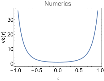
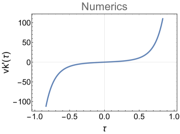
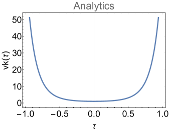
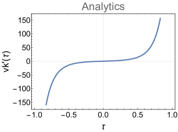
Figure 2: Comparison between the numerical solution to equation (4.18) (upper graphs) and its semi-analytical approximation (B.1) (lower graphs) during the bounce phase. The left and right graphs show $v_{k}$ and $v_{k}^{\prime}$, respectively. We have imposed initial conditions $v_{k}(0)=1$ and $v_{k}^{\prime}(0)=0$.

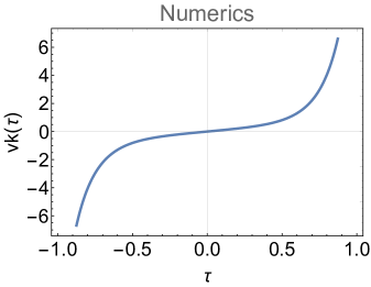
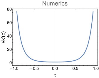
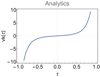
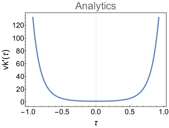
Figure 3: Comparison between the numerical solution to equation (4.18) (upper graphs) and its semi-analytical approximation (B.1) (lower graphs) during the bounce phase. The left and right graphs show $v_{k}$ and $v_{k}^{\prime}$, respectively. We have imposed initial conditions $v_{k}(0)=0$, $v_{k}^{\prime}(0)=1$.

For $v_{k}(0)=1~{},~{}v_{k}^{\prime}(0)=0$, the corresponding coefficients in (B.1) are $b_{s,3}=b_{s,4}=\frac{1}{2}$. In Fig. 2 we present the results. Similarly, for $v_{k}(0)=0~{},~{}v_{k}^{\prime}(0)=1$, the corresponding coefficients in (B.1) are $b_{s,3}=-b_{s,4}=\frac{1}{2\omega_{k}(0)}$, and in Fig. 3 we depict the resulting behavior. In both cases, we deduce that the numerical and analytical results are in perfect agreement, apart from an insignificant multiplication factor of the order $\mathcal{O}(1)$. Hence, equation (B.1) indeed provides a good approximation to the solution of (4.18), and thus we shall use equation (B.1) for the following calculations.

Appendix C Matching Conditions for Scalar Perturbations

In this Appendix we derive the matching conditions for scalar perturbations across the transition surface. The first matching surface is $\tau=\tau_{B-}$, and we shall match equation (4.13) with (4.21). At the time $\tau=\tau_{B-}$, the dominant part of (4.13) is the Bessel $Y$ function, therefore we may take

$$v_{k}^{c}(\tau)\simeq b_{s,2}\sqrt{\tau_{-}-\tau}Y_{\nu_{c}}[k(\tau_{-}-\tau)]\simeq-b_{s,2}\frac{\Gamma(\nu_{c})}{\pi}\left(\frac{2}{k}\right)^{\nu_{c}}(\tau_{-}-\tau)^{\frac{1}{2}-\nu_{c}}~{},$$ (C.1)

where $\Gamma(x)$ is the gamma function. Hence we obtain

$$v_{k}^{c}(\tau_{B-})\simeq-b_{s,2}\frac{\Gamma(\nu_{c})}{\pi}\left(\frac{2}{k}\right)^{\nu_{c}}(\tau_{-}-\tau_{B-})^{\frac{1}{2}-\nu_{c}}~{},$$ (C.2)

$$\frac{dv_{k}^{c}}{d\tau}(\tau_{B-})\simeq b_{s,2}\frac{\Gamma(\nu_{c})}{\pi}\left(\frac{1}{2}-\nu_{c}\right)\left(\frac{2}{k}\right)^{\nu_{c}}(\tau_{-}-\tau_{B-})^{-\frac{1}{2}-\nu_{c}}~{}.$$ (C.3)

As we analyzed in Section 4.3, the dynamics of scalar perturbations during the bounce phase can be simplified as

$$v_{k}^{b}(\tau)\simeq b_{s,3}e^{W_{k}(\tau)}+b_{s,4}e^{-W_{k}(\tau)}~{},~{}\frac{dv_{k}^{b}}{d\tau}(\tau)=\omega_{k}\left(b_{s,3}e^{W_{k}(\tau)}-b_{s,4}e^{W_{k}(\tau)}\right)~{},$$ (C.4)

with the help of the definition

$$W_{k}(\tau)\equiv\int_{\tau_{B-}}^{\tau}\omega_{k}(x)dx~{}\to~{}W_{k}^{\prime}(\tau)=\omega_{k}(\tau)~{}.$$ (C.5)

Note that here the lower limit of integration in $W_{k}(\tau)$ is taken as $\tau_{B-}$, different from the case of Appendix B above where the lower limit was 0. Since the change of the integration range can correspond to a redefinition of $b_{s,3}$ and $b_{s,4}$, equation (C.4) remains valid. Finally, for convenience we introduce the abbreviation

$$\omega_{k-}\equiv\omega_{k}(\tau_{B-})~{},~{}\omega_{k+}\equiv\omega_{k}(\tau_{B+})~{}.$$ (C.6)

The perturbation $v_{k}$ at the transition surface $\tau=\tau_{B-}$ can be found by directly substituting the time into equation (C.4). However, at $\tau=\tau_{B+}$ we observe that the $b_{s,4}$ term in transition surface $\tau=\tau_{B+}$ can be omitted: during the bounce phase, the $b_{s,4}$ term will be suppressed by a factor $\mathcal{F}_{s}$, while the $b_{s,3}$ term acquires an amplification by the same factor. The factor $\mathcal{F}_{s}$ is generally large (for example in the numerical case we have $\mathcal{F}_{s}\sim\mathcal{O}(10^{4})$) and depends on $k$. Hence, the $b_{s,4}$ term will be negligible at $\tau=\tau_{B+}$, and we have

$$v_{k}^{b}(\tau_{B+})\simeq b_{s,3}\mathcal{F}_{s}~{},~{}\frac{dv_{k}^{b}}{d\tau}(\tau_{B+})\simeq b_{s,3}\omega_{k+}\mathcal{F}_{s}~{},$$ (C.7)

where we have used the fact $\mathcal{F}_{s}\simeq W_{k}(\tau_{B+})$.

Finally, we use the small-argument expansion of the Bessel function to rewrite equation (4.29) at $\tau\to\tau_{B+}$ as

$$v_{k}^{e}(\tau)\simeq b_{s,5}\sqrt{\tau-\tau_{+}}+\frac{2}{\pi}\left[\ln\frac{k(\tau-\tau_{+})}{2}+\gamma_{E}\right]b_{s,6}\sqrt{\tau-\tau_{+}}~{},$$ (C.8)

where $\gamma_{E}\simeq 0.58$ is the Euler-Masheroni constant. At the transition surface $\tau=\tau_{B+}$, we have

$$v_{k}^{e}(\tau_{B+})\simeq b_{s,5}\sqrt{\tau_{B+}-\tau_{+}}+\frac{2}{\pi}\left[\ln\frac{k(\tau_{B+}-\tau_{+})}{2}+\gamma_{E}\right]b_{s,6}\sqrt{\tau_{B+}-\tau_{+}}~{},$$ (C.9)

$$\frac{dv_{k}^{e}}{d\tau}(\tau_{B+})=\frac{1}{2\sqrt{\tau_{B+}-\tau_{+}}}\left[b_{s,5}+\frac{2b_{s,6}}{\pi}\left(2+\gamma_{E}+\ln\frac{k(\tau_{B+}-\tau_{+})}{2}\right)\right]~{}.$$ (C.10)

Equating $v_{k}$ and $v_{k}^{\prime}$ at $\tau=\tau_{B-}$ and eliminating $b_{s,4}$, we have

$$b_{s,3}=\frac{b_{s,2}\Gamma(\nu_{c})\left[1-2\nu_{c}-2(\tau_{-}-,\tau_{B-})\omega_{k-}\right]}{2^{2-\nu_{c}}\pi k^{\nu_{c}}(\tau_{-}-\tau_{B-})^{\frac{1}{2}+\nu_{c}}\omega_{k-}}~{},$$ (C.11)

where we have used that $W_{k}(\tau_{B-})=0$ by definition. Determining $b_{s,3}$ is sufficient to extract all information about $v_{k}$ at $\tau=\tau_{B+}$. Moreover, we should acquire $b_{s,5}$ and $b_{s,6}$ in equation (4.29). Hence, equating $v_{k}$ and $v_{k}^{\prime}$ at $\tau=\tau_{B+}$ we obtain

$$b_{s,5}=\frac{b_{s,3}\mathcal{F}_{s}}{\sqrt{\tau_{B+}-\tau_{+}}}\left\{1-\left[(\tau_{B+}-\tau_{+})\omega_{k+}-\frac{1}{2}\right]\left[\ln\frac{k(\tau_{B+}-\tau_{+})}{2}+\gamma_{E}\right]\right\},$$ (C.12)

$$b_{s,6}=\frac{\pi}{4}\mathcal{F}_{s}b_{s,3}\frac{2(\tau_{B+}-\tau_{+})\omega_{k+}-1}{\sqrt{\tau_{B+}-\tau_{+}}}~{}.$$ (C.13)

Before proceeding, we replace the combination $(\tau_{B+}-\tau_{+})$ through the Hubble parameter $\mathcal{H}_{B+}$, which represents the energy scale at the end of the bounce phase, since from (3.12) we have $\tau_{B+}-\tau_{+}=\frac{1}{2\mathcal{H}_{B+}}$. Combining (C.11), (C.12) and (C.13), we can finally express the coefficients $b_{s,5}$, $b_{s,6}$ in terms of the initial condition $b_{s,2}$ as

$$b_{s,5}=\frac{\mathcal{F}_{s}\Gamma(\nu_{c})\left[1-2\nu_{c}-2(\tau_{-}-\tau_{B-})\omega_{k-}\right]}{2^{\frac{5}{2}-\nu_{c}}\pi k^{\nu_{c}}(\tau_{-}-\tau_{B-})^{\frac{1}{2}+\nu_{c}}\omega_{k-}\mathcal{H}_{B+}^{-1/2}}\left[2-\left(\frac{\omega_{k+}}{\mathcal{H}_{B+}}-1\right)\ln\frac{ke^{\gamma_{E}}}{4\mathcal{H}_{B+}}\right]b_{s,2}~{},$$ (C.14)

$$b_{s,6}=\frac{\mathcal{F}_{s}\Gamma(\nu_{c})}{2^{\frac{7}{2}-\nu_{c}}k^{\nu_{c}}}\frac{1-2\nu_{c}-2(\tau_{-}-\tau_{B-})\omega_{k-}}{(\tau_{-}-\tau_{B-})^{\frac{1}{2}+\nu_{c}}\omega_{k-}}\left[\frac{\omega_{k+}}{\sqrt{\mathcal{H}_{B+}}}-\sqrt{\mathcal{H}_{B+}}\right]b_{s,2}~{}.$$ (C.15)

Expressions (C.14) and (C.15) can be further simplified. Since we have a short bounce, $\mathcal{H}_{B+}$ and $\mathcal{H}_{B-}$ will have a relatively small value; in the specific case used in the main text of this manuscript, they are of the order of $10^{-4}$, thus $1/\mathcal{H}$ will be relatively large. On the other hand, for Ekpyrotic matter field we have $0<\nu_{c}<1/2$ since $0<q<1/3$, and $\omega_{k+}$ is of the order of $\mathcal{O}(10)$ (in our case $\omega_{k+}\simeq 8.5$). Hence, we can neglect the term $1-2\nu_{c}$ and $\mathcal{H}_{B+}/\omega_{k+}$, and the final expressions for $b_{s,5}$ and $b_{s,6}$ are

$$\frac{b_{s,5}}{b_{s,2}}=\frac{\mathcal{F}_{s}\Gamma\left(\nu_{c}\right)\left(1-2\nu_{c}\right)^{\frac{1}{2}-\nu_{c}}}{4^{1-\nu_{c}}\pi}\left(\frac{-\mathcal{H}_{B-}}{k}\right)^{\nu_{c}}\left(\frac{w_{k+}}{\sqrt{-\mathcal{H}_{B-}\mathcal{H}_{B+}}}\ln\frac{ke^{\gamma_{E}}}{4\mathcal{H}_{B+}}-\sqrt{\frac{4\mathcal{H_{B+}}}{-\mathcal{H_{B-}}}}\right)~{},$$ (C.16)

and

$$\frac{b_{s,6}}{b_{s,2}}=-\frac{\mathcal{F}_{s}\Gamma(\nu_{c})(1-2\nu_{c})^{\frac{1}{2}-\nu_{c}}}{2^{3-2\nu_{c}}}\left(\frac{-\mathcal{H_{B-}}}{k}\right)^{\nu_{c}}\frac{\omega_{k+}}{\sqrt{-\mathcal{H_{B-}}\mathcal{H_{B+}}}}~{},$$ (C.17)

where we have used that

$$\tau_{-}-\tau_{B-}=-\frac{q}{(1-q)\mathcal{H_{B-}}}~{}.$$ (C.18)

Equations (C.16) and (C.17) are the final results of this Appendix.

Appendix D Matching Conditions for Tensor Perturbations

In this Appendix we first deduce the matching conditions for tensor perturbations across the transition surface, and then we apply it to our model. The starting point is the MS equation (4.8), which can be rewritten as

$$\frac{d}{d\tau}\left(\mu_{k}^{\prime}a-\mu_{k}a^{\prime}\right)=-c_{T}^{2}k^{2}a\mu_{k}~{}.$$ (D.1)

Only for this Appendix we define the auxiliary functions

$$g(\tau)=\mu_{k}^{\prime}(\tau)a(\tau)-\mu_{k}(\tau)a^{\prime}(\tau)~{},~{}M(\tau,\epsilon_{1},\epsilon_{2})=\int_{\tau-\epsilon_{2}}^{\tau+\epsilon_{1}}[-c_{T}^{2}k^{2}a(\tau)\mu_{k}(\tau)]d\tau~{},$$ (D.2)

and thus when we integrate equation (D.1) across one transition surface, e.g. $\tau=\tau_{B-}$, we obtain

$$g(\tau_{B-}+\epsilon_{1})-g(\tau_{B-}-\epsilon_{2})=M(\tau_{B-},\epsilon_{1},\epsilon_{2})~{}.$$ (D.3)

From the finiteness of $a(\tau)$ and $\mu_{k}(\tau)$, it is easy to see that

$$\lim_{\epsilon_{1}\to 0,\epsilon_{2}\to 0}M(\tau_{B-},\epsilon_{1},\epsilon_{2})=0~{},$$ (D.4)

and therefore $g(\tau)$ should be finite near the transition surface, otherwise the limiting value of $M$ would be a finite number. Then integrating (D.3) we have

$$\left(\frac{\mu_{k}}{a}\right)(\tau_{B-}+\lambda)-\left(\frac{\mu_{k}}{a}\right)(\tau_{B-}-\lambda)=\int_{\tau_{B-}-\lambda}^{\tau_{B-}+\lambda}[a(\tau)^{2}g(\tau)]d\tau~{}.$$ (D.5)

As we can see, in the limit $\lambda\to 0$ the right-hand-side of (D.5) will vanish due to the finiteness of $a(\tau)$ and $g(\tau)$. Hence, $\mu_{k}/a$ is continuous at $\tau=\tau_{B-}$, and alongside the continuity of $a(\tau)$ we deduce that $\mu_{k}(\tau)$ is continuous at $\tau=\tau_{B-}$. Finally, looking at (D.3), and following the same argument, we find that $g(\tau)$ is continuous at $\tau=\tau_{B-}$. Now since $a(\tau)$, $a^{\prime}(\tau)$ and $\mu_{k}(\tau)$ are continuous at the transition surface, we immediately deduce the continuity of $\mu_{k}^{\prime}(\tau)$.

Hence we extract the matching conditions for tensor perturbations: $\mu_{k}$ and $\mu_{k}^{\prime}$ are continuous at the transition surface $\tau=\tau_{B-}$ and $\tau=\tau_{B+}$. In the present case $\mu_{k}$ and $\mu_{k}^{\prime}$ remain almost invariant during the bounce phase, therefore we can directly match $\mu_{k}^{c}(\tau_{B-})$ and $\mu_{k}^{\prime c}(\tau_{B-})$ with $\mu_{k}^{e}(\tau_{B+})$ and $\mu_{k}^{\prime e}(\tau_{B+})$.

At $\tau=\tau_{B-}$ the tensor perturbations and derivative behave as

$$\mu_{k}^{c}(\tau_{B-})\simeq-b_{t,2}\frac{\Gamma(\nu_{c})}{\pi}\left(\frac{2}{k}\right)^{\nu_{c}}(\tau_{-}-\tau_{B-})^{\frac{1}{2}-\nu_{c}}~{},$$ (D.6)

$$\frac{d\mu_{k}^{c}}{d\tau}(\tau_{B-})\simeq b_{t,2}\frac{\Gamma(\nu_{c})}{\pi}\left(\frac{1}{2}-\nu_{c}\right)\left(\frac{2}{k}\right)^{\nu_{c}}(\tau_{-}-\tau_{B-})^{-\frac{1}{2}-\nu_{c}}~{},$$ (D.7)

similarly to the scalar case. At the transition surface $\tau=\tau_{B+}$ we have

$$\mu_{k}^{e}(\tau_{B+})=b_{t,5}\sqrt{\tau_{B+}-\tau_{+}}+\frac{2}{\pi}\left[\ln\frac{k(\tau_{B+}-\tau_{+})}{2}+\gamma_{E}\right]b_{t,6}\sqrt{\tau_{B+}-\tau_{+}}~{},$$ (D.8)

$$\frac{d\mu_{k}^{e}}{d\tau}(\tau_{B+})=\frac{1}{2\sqrt{\tau_{B+}-\tau_{+}}}\left[b_{t,5}+\frac{2b_{t,6}}{\pi}\left(2+\gamma_{E}+\ln\frac{k(\tau_{B+}-\tau_{+})}{2}\right)\right]~{}.$$ (D.9)

Using $\mu_{k}^{c}(\tau_{B-})=\mu_{k}^{e}(\tau_{B+})$, $\frac{d\mu_{k}^{c}}{d\tau}(\tau_{B-})=\frac{d\mu_{k}^{e}}{d\tau}(\tau_{B+})$, we acquire

$$b_{t,6}=\frac{\Gamma(\nu_{c})2^{\nu_{c}-2}}{k^{\nu_{c}}\sqrt{\tau_{B+}-\tau_{+}}(\tau_{-}-\tau_{B-})^{\frac{1}{2}+\nu_{c}}}\left[(1-2\nu_{c})(\tau_{B+}-\tau_{+})+(\tau_{-}-\tau_{B-})\right]b_{t,2}~{}.$$ (D.10)

We can simplify this relation by using

$$\tau_{B+}-\tau_{+}=\frac{1}{2\mathcal{H}_{B+}}~{},~{}\tau_{-}-\tau_{B-}=-\frac{q}{(1-q)\mathcal{H}_{B-}}~{},~{}\mathcal{H}_{B-}\simeq-\mathcal{H}_{B+}~{},$$ (D.11)

obtaining

$$\frac{b_{t,6}}{b_{t,2}}=\frac{\left(1-2\nu_{c}\right)^{\frac{1}{2}-\nu_{c}}\Gamma\left(\nu_{c}\right)}{4^{1-\nu_{c}}}\sqrt{\frac{\mathcal{H}_{B+}}{-\mathcal{H}_{B-}}}\left(1+\frac{-\mathcal{H}_{B-}}{\mathcal{H}_{B+}}\right)\left(\frac{-\mathcal{H}_{B-}}{k}\right)^{\nu_{c}}b_{t,2}~{},$$ (D.12)

$$\frac{b_{t,5}}{b_{t,2}}=\frac{-\left(1-2\nu_{c}\right)^{\frac{1}{2}-\nu_{c}}\Gamma\left(\nu_{c}\right)}{2^{1-2\nu_{c}}\pi}\sqrt{\frac{\mathcal{H}_{B+}}{-\mathcal{H}_{B-}}}\left[2+\left(1+\frac{-\mathcal{H}_{B-}}{\mathcal{H}_{B+}}\right)\ln\frac{ke^{\gamma_{E}}}{4\mathcal{H}_{B+}}\right]\left(\frac{-\mathcal{H}_{B-}}{k}\right)^{\nu_{c}}~{}.$$ (D.13)

Expressions (D.12) and (D.13) are the final results of this Appendix.

References

- [1] M. Novello and S. E. P. Bergliaffa, Bouncing Cosmologies, Phys. Rept. 463, 127 (2008) [arXiv:0802.1634 [astro-ph]].
- [2] J. L. Lehners, Ekpyrotic and Cyclic Cosmology, Phys. Rept. 465, 223 (2008) [arXiv:0806.1245 [astro-ph]].
- [3] Y. F. Cai, Exploring Bouncing Cosmologies with Cosmological Surveys, Sci. China Phys. Mech. Astron. 57, 1414 (2014) [arXiv:1405.1369 [hep-th]].
- [4] D. Battefeld and P. Peter, A Critical Review of Classical Bouncing Cosmologies, Phys. Rept. 571, 1 (2015) [arXiv:1406.2790 [astro-ph.CO]].
- [5] R. Brandenberger and P. Peter, Bouncing Cosmologies: Progress and Problems, Found. Phys. 47, no. 6, 797 (2017) [arXiv:1603.05834 [hep-th]].
- [6] Y. F. Cai, A. Marciano, D. G. Wang and E. Wilson-Ewing, Bouncing cosmologies with dark matter and dark energy, Universe 3, no. 1, 1 (2016) [arXiv:1610.00938 [astro-ph.CO]].
- [7] R. H. Brandenberger, Introduction to Early Universe Cosmology, PoS ICFI2010, 001 (2010) [arXiv:1103.2271 [astro-ph.CO]].
- [8] A. Borde and A. Vilenkin, Eternal inflation and the initial singularity, Phys. Rev. Lett. 72, 3305 (1994) [gr-qc/9312022].
- [9] A. Borde, A. H. Guth and A. Vilenkin, Inflationary space-times are incompletein past directions, Phys. Rev. Lett. 90, 151301 (2003) [gr-qc/0110012].
- [10] J. M. Cline, S. Jeon and G. D. Moore, The Phantom menaced: Constraints on low-energy effective ghosts, Phys. Rev. D 70, 043543 (2004) [hep-ph/0311312].
- [11] D. A. Easson and A. Vikman, The Phantom of the New Oscillatory Cosmological Phase, [arXiv:1607.00996 [gr-qc]].
- [12] J. Q. Xia, Y. F. Cai, T. T. Qiu, G. B. Zhao and X. Zhang, Constraints on the Sound Speed of Dynamical Dark Energy, Int. J. Mod. Phys. D 17, 1229-1243 (2008) [arXiv:astro-ph/0703202 [astro-ph]].
- [13] A. Vikman, Can dark energy evolve to the phantom?, Phys. Rev. D 71, 023515 (2005) [astro-ph/0407107].
- [14] J. Karouby and R. Brandenberger, A Radiation Bounce from the Lee-Wick Construction?, Phys. Rev. D 82, 063532 (2010) [arXiv:1004.4947 [hep-th]].
- [15] J. Karouby, T. Qiu and R. Brandenberger, On the Instability of the Lee-Wick Bounce, Phys. Rev. D 84, 043505 (2011) [arXiv:1104.3193 [hep-th]].
- [16] K. Bhattacharya, Y. F. Cai and S. Das, Lee-Wick radiation induced bouncing universe models, Phys. Rev. D 87, no. 8, 083511 (2013) [arXiv:1301.0661 [hep-th]].
- [17] Y. F. Cai, R. Brandenberger and P. Peter, Anisotropy in a Nonsingular Bounce, Class. Quant. Grav. 30, 075019 (2013) [arXiv:1301.4703 [gr-qc]].
- [18] V. A. Belinsky, I. M. Khalatnikov and E. M. Lifshitz, Oscillatory approach to a singular point in the relativistic cosmology, Adv. Phys. 19, 525 (1970).
- [19] Y. F. Cai, W. Xue, R. Brandenberger and X. Zhang, Non-Gaussianity in a Matter Bounce, JCAP 0905, 011 (2009) [arXiv:0903.0631 [astro-ph.CO]].
- [20] X. Gao, M. Lilley and P. Peter, Production of non-gaussianities through a positive spatial curvature bouncing phase, JCAP 1407, 010 (2014) [arXiv:1403.7958 [gr-qc]].
- [21] X. Gao, M. Lilley and P. Peter, Non-Gaussianity excess problem in classical bouncing cosmologies, Phys. Rev. D 91, no. 2, 023516 (2015) [arXiv:1406.4119 [gr-qc]].
- [22] J. Quintin, Z. Sherkatghanad, Y. F. Cai and R. H. Brandenberger, Evolution of cosmological perturbations and the production of non-Gaussianities through a nonsingular bounce: Indications for a no-go theorem in single field matter bounce cosmologies, Phys. Rev. D 92, no. 6, 063532 (2015) [arXiv:1508.04141 [hep-th]].
- [23] Y. B. Li, J. Quintin, D. G. Wang and Y. F. Cai, Matter bounce cosmology with a generalized single field: non-Gaussianity and an extended no-go theorem, JCAP 1703, 031 (2017) [arXiv:1612.02036 [hep-th]].
- [24] S. Akama, S. Hirano and T. Kobayashi, Primordial non-Gaussianities of scalar and tensor perturbations in general bounce cosmology: Evading the no-go theorem, Phys. Rev. D 101, no.4, 043529 (2020) [arXiv:1908.10663 [gr-qc]].
- [25] K. S. Kumar, S. Maheshwari, A. Mazumdar and J. Peng, An anisotropic bouncing universe in non-local gravity, JCAP 07 (2021), 025 [arXiv:2103.13980 [gr-qc]].
- [26] N. Pinto-Neto, Bouncing Quantum Cosmology, Universe 7 (2021) no.4, 110
- [27] D. Nandi, Stability of a viable non-minimal bounce, Universe 7, no.3, 62 (2021) [arXiv:2009.03134 [gr-qc]].
- [28] Y. Cai, Y. Wan, H. G. Li, T. Qiu and Y. S. Piao, The Effective Field Theory of nonsingular cosmology, JHEP 01, 090 (2017) [arXiv:1610.03400 [gr-qc]].
- [29] P. Creminelli, D. Pirtskhalava, L. Santoni and E. Trincherini, Stability of Geodesically Complete Cosmologies, JCAP 11, 047 (2016) [arXiv:1610.04207 [hep-th]].
- [30] Y. Cai, H. G. Li, T. Qiu and Y. S. Piao, The Effective Field Theory of nonsingular cosmology: II, Eur. Phys. J. C 77, no.6, 369 (2017) [arXiv:1701.04330 [gr-qc]].
- [31] Y. Cai, Y. T. Wang, J. Y. Zhao and Y. S. Piao, Primordial perturbations with pre-inflationary bounce, Phys. Rev. D 97, no.10, 103535 (2018) [arXiv:1709.07464 [astro-ph.CO]].
- [32] R. Kolevatov, S. Mironov, N. Sukhov and V. Volkova, Cosmological bounce and Genesis beyond Horndeski, JCAP 08, 038 (2017) [arXiv:1705.06626 [hep-th]].
- [33] Y. Cai and Y. S. Piao, A covariant Lagrangian for stable nonsingular bounce, JHEP 09, 027 (2017) [arXiv:1705.03401 [gr-qc]].
- [34] G. Ye and Y. S. Piao, Implication of GW170817 for cosmological bounces, Commun. Theor. Phys. 71, no.4, 427 (2019) [arXiv:1901.02202 [gr-qc]].
- [35] G. Ye and Y. S. Piao, Bounce in general relativity and higher-order derivative operators, Phys. Rev. D 99, no.8, 084019 (2019) [arXiv:1901.08283 [gr-qc]].
- [36] Ö. Güngör and G. D. Starkman, A classical, non-singular, bouncing universe, JCAP 04 (2021), 003 [arXiv:2011.05133 [gr-qc]].
- [37] Y. Zheng, L. Shen, Y. Mou and M. Li, On (in)stabilities of perturbations in mimetic models with higher derivatives, JCAP 08, 040 (2017) [arXiv:1704.06834 [gr-qc]].
- [38] M. Libanov, S. Mironov and V. Rubakov, Generalized Galileons: instabilities of bouncing and Genesis cosmologies and modified Genesis, JCAP 08, 037 (2016) [arXiv:1605.05992 [hep-th]].
- [39] T. Kobayashi, Generic instabilities of nonsingular cosmologies in Horndeski theory: A no-go theorem, Phys. Rev. D 94, no.4, 043511 (2016) [arXiv:1606.05831 [hep-th]].
- [40] S. Akama and T. Kobayashi, Generalized multi-Galileons, covariantized new terms, and the no-go theorem for nonsingular cosmologies, Phys. Rev. D 95, no.6, 064011 (2017) [arXiv:1701.02926 [hep-th]].
- [41] J. Khoury, B. A. Ovrut, P. J. Steinhardt and N. Turok, The Ekpyrotic universe: Colliding branes and the origin of the hot big bang, Phys. Rev. D 64, 123522 (2001) [arXiv:hep-th/0103239 [hep-th]].
- [42] A. Ilyas, M. Zhu, Y. Zheng, Y. F. Cai and E. N. Saridakis, DHOST Bounce, JCAP 09, 002 (2020) [arXiv:2002.08269 [gr-qc]].
- [43] A. Nicolis, R. Rattazzi and E. Trincherini, The Galileon as a local modification of gravity, Phys. Rev. D 79, 064036 (2009) [arXiv:0811.2197 [hep-th]].
- [44] C. Deffayet, X. Gao, D. A. Steer and G. Zahariade, From k-essence to generalised Galileons, Phys. Rev. D 84, 064039 (2011) [arXiv:1103.3260 [hep-th]].
- [45] T. Kobayashi, M. Yamaguchi and J. Yokoyama, Generalized G-inflation: Inflation with the most general second-order field equations, Prog. Theor. Phys. 126, 511-529 (2011) [arXiv:1105.5723 [hep-th]].
- [46] G. W. Horndeski, Second-order scalar-tensor field equations in a four-dimensional space, Int. J. Theor. Phys. 10, 363-384 (1974)
- [47] T. Kobayashi, M. Yamaguchi and J. Yokoyama, G-inflation: Inflation driven by the Galileon field, Phys. Rev. Lett. 105, 231302 (2010) [arXiv:1008.0603 [hep-th]].
- [48] C. Deffayet, O. Pujolas, I. Sawicki and A. Vikman, Imperfect Dark Energy from Kinetic Gravity Braiding, JCAP 10, 026 (2010) [arXiv:1008.0048 [hep-th]].
- [49] T. Qiu, J. Evslin, Y. F. Cai, M. Li and X. Zhang, Bouncing Galileon Cosmologies, JCAP 10, 036 (2011) [arXiv:1108.0593 [hep-th]].
- [50] D. A. Easson, I. Sawicki and A. Vikman, G-Bounce, JCAP 11, 021 (2011) [arXiv:1109.1047 [hep-th]].
- [51] Y. F. Cai, D. A. Easson and R. Brandenberger, Towards a Nonsingular Bouncing Cosmology, JCAP 08, 020 (2012) [arXiv:1206.2382 [hep-th]].
- [52] G. Leon and E. N. Saridakis, Dynamical analysis of generalized Galileon cosmology, JCAP 03, 025 (2013) [arXiv:1211.3088 [astro-ph.CO]].
- [53] E. N. Saridakis et al. [CANTATA], Modified Gravity and Cosmology: An Update by the CANTATA Network, [arXiv:2105.12582 [gr-qc]].
- [54] M. Ostrogradsky, Mémoires sur les équations différentielles, relatives au problème des isopérimètres, Mem. Acad. St. Petersbourg 6, no.4, 385-517 (1850)
- [55] O. S. An, J. U. Kang, T. H. Kim and U. R. Mun, Notes on the post-bounce background dynamics in bouncing cosmologies, [arXiv:2010.13287 [gr-qc]].
- [56] R. Brandenberger, Q. Liang, R. O. Ramos and S. Zhou, Fluctuations through a Vibrating Bounce, Phys. Rev. D 97, no.4, 043504 (2018) [arXiv:1711.08370 [hep-th]].
- [57] S. Mironov, V. Rubakov and V. Volkova, Superluminality in beyond Horndeski theory with extra scalar field, Phys. Scripta 95, no.8, 084002 (2020) [arXiv:2005.12626 [hep-th]].
- [58] S. Mironov, V. Rubakov and V. Volkova, Superluminality in DHOST theory with extra scalar, JHEP 04, 035 (2021) [arXiv:2011.14912 [hep-th]].
- [59] C. Jonas, J. L. Lehners and J. Quintin, Cosmological consequences of a principle of finite amplitudes, Phys. Rev. D 103, no.10, 103525 (2021) [arXiv:2102.05550 [hep-th]].
- [60] Y. F. Cai, T. Qiu, R. Brandenberger, Y. S. Piao and X. Zhang, On Perturbations of Quintom Bounce, JCAP 03, 013 (2008) [arXiv:0711.2187 [hep-th]].
- [61] Y. F. Cai and X. Zhang, Evolution of Metric Perturbations in Quintom Bounce model, JCAP 06, 003 (2009) [arXiv:0808.2551 [astro-ph]].
- [62] Y. F. Cai, T. t. Qiu, R. Brandenberger and X. m. Zhang, A Nonsingular Cosmology with a Scale-Invariant Spectrum of Cosmological Perturbations from Lee-Wick Theory, Phys. Rev. D 80, 023511 (2009) [arXiv:0810.4677 [hep-th]].
- [63] C. Lin, R. H. Brandenberger and L. Perreault Levasseur, A Matter Bounce By Means of Ghost Condensation, JCAP 04, 019 (2011) [arXiv:1007.2654 [hep-th]].
- [64] A. Ilyas, M. Zhu, Y. Zheng and Y. F. Cai, Emergent Universe and Genesis from the DHOST Cosmology, JHEP 01, 141 (2021) [arXiv:2009.10351 [gr-qc]].
- [65] M. Zhu and Y. Zheng, Improved DHOST Genesis, [arXiv:2109.05277 [gr-qc]].
- [66] M. Sasaki, Gauge Invariant Scalar Perturbations in the New Inflationary Universe, Prog. Theor. Phys. 70, 394 (1983)
- [67] H. Kodama and M. Sasaki, Cosmological Perturbation Theory, Prog. Theor. Phys. Suppl. 78, 1-166 (1984)
- [68] V. F. Mukhanov, Quantum Theory of Gauge Invariant Cosmological Perturbations, Sov. Phys. JETP 67, 1297-1302 (1988)
- [69] Y. F. Cai, J. Quintin, E. N. Saridakis and E. Wilson-Ewing, Nonsingular bouncing cosmologies in light of BICEP2, JCAP 07, 033 (2014) [arXiv:1404.4364 [astro-ph.CO]].
- [70] S. Banerjee and E. N. Saridakis, Bounce and cyclic cosmology in weakly broken galileon theories, Phys. Rev. D 95, no.6, 063523 (2017) [arXiv:1604.06932 [gr-qc]].
- [71] J. c. Hwang and E. T. Vishniac, Gauge-invariant joining conditions for cosmological perturbations, Astrophys. J. 382, 363-368 (1991)
- [72] N. Deruelle and V. F. Mukhanov, On matching conditions for cosmological perturbations, Phys. Rev. D 52, 5549-5555 (1995) [arXiv:gr-qc/9503050 [gr-qc]].
- [73] P. Creminelli, K. Hinterbichler, J. Khoury, A. Nicolis and E. Trincherini, Subluminal Galilean Genesis, JHEP 02, 006 (2013) [arXiv:1209.3768 [hep-th]].
- [74] K. Hinterbichler, A. Joyce, J. Khoury and G. E. J. Miller, Dirac-Born-Infeld Genesis: An Improved Violation of the Null Energy Condition, Phys. Rev. Lett. 110, no.24, 241303 (2013) [arXiv:1212.3607 [hep-th]].
- [75] A. Padilla and V. Sivanesan, Boundary Terms and Junction Conditions for Generalized Scalar-Tensor Theories, JHEP 08, 122 (2012) [arXiv:1206.1258 [gr-qc]].
- [76] S. Nishi, T. Kobayashi, N. Tanahashi and M. Yamaguchi, Cosmological matching conditionsand galilean genesis in Horndeski’s theory, JCAP 03, 008 (2014) [arXiv:1401.1045 [hep-th]].
- [77] L. Avilés, H. Maeda and C. Martinez, Junction conditions in scalar–tensor theories, Class. Quant. Grav. 37, no.7, 075022 (2020) [arXiv:1910.07534 [gr-qc]].
- [78] E. N. Saridakis, Do we need soft cosmology?, [arXiv:2105.08646 [astro-ph.CO]].
- [79] D. H. Lyth, The Primordial curvature perturbation in the ekpyrotic universe, Phys. Lett. B 524, 1-4 (2002) [arXiv:hep-ph/0106153 [hep-ph]].
- [80] R. Brandenberger and F. Finelli, On the spectrum of fluctuations in an effective field theory of the Ekpyrotic universe, JHEP 11, 056 (2001) [arXiv:hep-th/0109004 [hep-th]].
- [81] S. Tsujikawa, R. Brandenberger and F. Finelli, On the construction of nonsingular pre - big bang and ekpyrotic cosmologies and the resulting density perturbations, Phys. Rev. D 66, 083513 (2002) [arXiv:hep-th/0207228 [hep-th]].
- [82] A. J. Tolley, N. Turok and P. J. Steinhardt, Cosmological perturbations in a big crunch / big bang space-time, Phys. Rev. D 69, 106005 (2004) [arXiv:hep-th/0306109 [hep-th]].
- [83] A. Notari and A. Riotto, Isocurvature perturbations in the ekpyrotic universe, Nucl. Phys. B 644, 371-382 (2002) [arXiv:hep-th/0205019 [hep-th]].
- [84] F. Finelli, Assisted contraction, Phys. Lett. B 545, 1-7 (2002) [arXiv:hep-th/0206112 [hep-th]].
- [85] P. Creminelli and L. Senatore, A Smooth bouncing cosmology with scale invariant spectrum, JCAP 11, 010 (2007) [arXiv:hep-th/0702165 [hep-th]].
- [86] J. L. Lehners, P. McFadden, N. Turok and P. J. Steinhardt, Generating ekpyrotic curvature perturbations before the big bang, Phys. Rev. D 76, 103501 (2007) [arXiv:hep-th/0702153 [hep-th]].
- [87] E. I. Buchbinder, J. Khoury and B. A. Ovrut, New Ekpyrotic cosmology, Phys. Rev. D 76, 123503 (2007) [arXiv:hep-th/0702154 [hep-th]].
- [88] T. J. Battefeld, S. P. Patil and R. H. Brandenberger, On the transfer of metric fluctuations when extra dimensions bounce or stabilize, Phys. Rev. D 73, 086002 (2006) [arXiv:hep-th/0509043 [hep-th]].
- [89] D. Wands, Duality invariance of cosmological perturbation spectra, Phys. Rev. D 60, 023507 (1999) [arXiv:gr-qc/9809062 [gr-qc]].
- [90] R. Durrer and F. Vernizzi, Adiabatic perturbations in pre - big bang models: Matching conditions and scale invariance, Phys. Rev. D 66, 083503 (2002) [arXiv:hep-ph/0203275 [hep-ph]].
- [91] Y. F. Cai, E. McDonough, F. Duplessis and R. H. Brandenberger, Two Field Matter Bounce Cosmology, JCAP 10, 024 (2013) [arXiv:1305.5259 [hep-th]].
- [92] N. Aghanim et al. [Planck], Planck 2018 results. VI. Cosmological parameters, Astron. Astrophys. 641, A6 (2020) [arXiv:1807.06209 [astro-ph.CO]].
- [93] Y. F. Cai, W. Xue, R. Brandenberger and X. m. Zhang, Thermal Fluctuations and Bouncing Cosmologies, JCAP 06, 037 (2009) [arXiv:0903.4938 [hep-th]].
- [94] K. Enqvist and M. S. Sloth, Adiabatic CMB perturbations in pre - big bang string cosmology, Nucl. Phys. B 626, 395-409 (2002) [arXiv:hep-ph/0109214 [hep-ph]].
- [95] D. H. Lyth and D. Wands, Generating the curvature perturbation without an inflaton, Phys. Lett. B 524, 5-14 (2002) [arXiv:hep-ph/0110002 [hep-ph]].
- [96] Y. F. Cai, R. Brandenberger and X. Zhang, The Matter Bounce Curvaton Scenario, JCAP 03, 003 (2011) [arXiv:1101.0822 [hep-th]].
- [97] Y. F. Cai, R. Brandenberger and X. Zhang, Preheating a bouncing universe, Phys. Lett. B 703, 25-33 (2011) [arXiv:1105.4286 [hep-th]].
- [98] H. W. H. Tahara and T. Kobayashi, Nanohertz gravitational waves from a null-energy-condition violation in the early universe, Phys. Rev. D 102, no.12, 123533 (2020) [arXiv:2011.01605 [gr-qc]].
- [99] Y. Cai and Y. S. Piao, Intermittent null energy condition violations during inflation and primordial gravitational waves, Phys. Rev. D 103, no.8, 083521 (2021) [arXiv:2012.11304 [gr-qc]].