AdvRush: Searching for Adversarially Robust Neural Architectures

Abstract

Deep neural networks continue to awe the world with their remarkable performance. Their predictions, however, are prone to be corrupted by adversarial examples that are imperceptible to humans. Current efforts to improve the robustness of neural networks against adversarial examples are focused on developing robust training methods, which update the weights of a neural network in a more robust direction. In this work, we take a step beyond training of the weight parameters and consider the problem of designing an adversarially robust neural architecture with high intrinsic robustness. We propose AdvRush, a novel adversarial robustness-aware neural architecture search algorithm, based upon a finding that independent of the training method, the intrinsic robustness of a neural network can be represented with the smoothness of its input loss landscape. Through a regularizer that favors a candidate architecture with a smoother input loss landscape, AdvRush successfully discovers an adversarially robust neural architecture. Along with a comprehensive theoretical motivation for AdvRush, we conduct an extensive amount of experiments to demonstrate the efficacy of AdvRush on various benchmark datasets. Notably, on CIFAR-10, AdvRush achieves 55.91% robust accuracy under FGSM attack after standard training and 50.04% robust accuracy under AutoAttack after 7-step PGD adversarial training.

1 Introduction

The rapid growth and integration of deep neural networks in every-day applications have led researchers to explore the susceptibility of their predictions to malicious external attacks. Among proposed attack mechanisms, adversarial examples [65], in particular, raise serious security concerns because they can cause neural networks to make erroneous predictions with the slightest perturbations in the input data that are indistinguishable to the human eyes. This interesting property of adversarial examples has been drawing much attention from the deep learning community, and ever since their introduction, a plethora of defense methods have been proposed to improve the robustness of neural networks against adversarial examples [75, 69, 36]. However, there remains one important question that is yet to be explored extensively: Can the adversarial robustness of a neural network be improved by utilizing an architecture with high intrinsic robustness? And if so, is it possible to automatically search for a robust neural architecture?

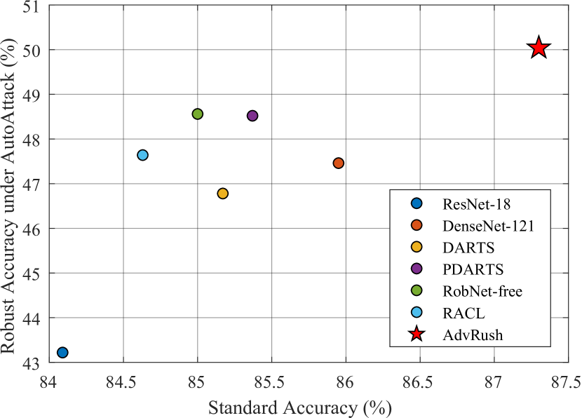
Figure 1: Standard accuracy vs. robust accuracy evaluation results on CIFAR-10 for various neural architectures and the neural architecture searched by AdvRush. All architectures are adversarially trained using 7-step PGD and evaluated under AutoAttack. AdvRush architecture achieves both standard accuracy-wise and robust accuracy-wise optimal frontiers.

We tackle the problem of searching for a robust neural architecture by employing Neural Architecture Search (NAS) [79]. Due to the heuristic nature of designing a neural architecture, it used to take machine learning engineers with years of experience and expertise to fully exploit the power of neural networks. NAS, a newly budding branch of automated machine learning, aims to automate this labor-intensive architecture search process. As the neural architectures discovered automatically through NAS begin to outperform hand-crafted architectures across various domains [9, 49, 77, 66, 44], more emphasis is being placed on the proper choice of an architecture to improve the performance of a neural network on a target task.

The primary objective of the existing NAS algorithms is concentrated on improving the standard accuracy, and thus, they do not consider the robustness of the searched architecture during the search process. Consequently, they provide no guarantee of robustness for the searched architecture, since the “no free lunch” theorem for adversarial robustness prevents neural networks from obtaining sufficient robustness without additional effort [15, 5, 78]. In addition, the trade-off between the standard accuracy and the adversarial robustness indicates that maximizing the standard accuracy and the adversarial robustness cannot go hand in hand [67], further necessitating a NAS algorithm designed specifically for adversarial robustness.

In this work, we propose a novel adversarial robustness-aware NAS algorithm, named AdvRush, which is a shorthand for “Adversarially Robust Architecture Rush.” AdvRush is inspired by a finding that the degree of curvature in the neural network’s input loss landscape is highly correlated with intrinsic robustness, regardless of how its weights are trained [78]. Therefore, by favoring a candidate architecture with a smoother input loss landscape during the search phase, AdvRush discovers a neural architecture with high intrinsic robustness. As shown in Figure 1, after undergoing an identical adversarial training procedure, the searched architecture of AdvRush simultaneously achieves the best standard and robust accuracies on CIFAR-10.

We provide comprehensive experimental results to demonstrate that the architecture searched by AdvRush is indeed equipped with high intrinsic robustness. On CIFAR-10, standard-trained AdvRush achieves 55.91% robust accuracy (2.50% improvement from PDARTS [9]) under FGSM, and adversarially-trained AdvRush achieves 50.04% robust accuracy (3.04% improvement from RobNet-free [24]) under AutoAttack. Furthermore, we evaluate the robust accuracy of AdvRush on CIFAR-100, SVHN, and Tiny-ImageNet to investigate its transferability; across all datasets, AdvRush consistently shows a substantial increase in the robust accuracy compared to other architectures. For the sake of reproducibility, we have included the code and representative model files of AdvRush in the supplementary materials.

Our contributions can be summarized as follows:

• We propose AdvRush, a novel NAS algorithm for discovering a robust neural architecture. Because AdvRush does not require independent adversarial training of candidate architectures for evaluation, its search process is highly efficient.

• The effectiveness of AdvRush is demonstrated through comprehensive evaluation under a number of adversarial attacks. Furthermore, we validate the transferability of AdvRush to various benchmark datasets.

• We provide extensive theoretical justification for AdvRush and complement it with the visual analysis of the discovered architecture. In addition, we provide a meaningful insight into what makes a neural architecture more robust against adversarial perturbations.

2 Related Works

2.1 Adversarial Attacks and Defenses

Adversarial attack methods can be divided into white-box and black-box attacks. Under the white-box setting [53, 47, 35, 46, 68], the attacker has full access to the target model, including its architecture and weights. FGSM [20], PGD [40], and CW [6] attacks are the famous white-box attacks, popularly used to evaluate the robustness of a neural network. On the contrary, under the black-box setting, the attacker has limited to no access to the target model. Thus, black-box attacks rely on a substitute model [52] or the target model’s prediction score [7, 4, 64, 22, 27, 45] to construct adversarial examples.

In response, numerous adversarial defense methods have been proposed to alleviate the vulnerability of neural networks to adversarial examples. Adversarial training [20] is known to be the most effective defense method. By utilizing adversarial examples as training data, adversarial training plays a min-max game; while the inner maximum produces stronger adversarial examples to maximize the cross-entropy loss, the outer minimum updates the model parameters to minimize it. A large number of defenses now adopt some form of regularization or adversarial training to improve robustness [31, 43, 59, 74, 75, 48, 55]. Our work is closely related to the defense approaches that utilize a regularization term derived from the curvature information of the neural network’s loss landscape to mimic the effect of adversarial training [48, 55].

Apart from adversarial training, feature denoising [42, 41, 60, 69, 71] has also been proven to be effective at improving the robustness of a neural network. Although gradient masking [62, 51] may appear to be a viable defense method, it can easily be circumvented by attacks based on approximate gradients [1, 12].

2.2 Neural Architecture Search

Early NAS algorithms based on evolutionary algorithm (EA) [58, 57] or reinforcement learning (RL) [79, 80, 2] often required thousands of GPU hours to search for an architecture, making their immediate application difficult. The majority of the computational overhead in these algorithms was caused by the need to train each candidate architecture to convergence and evaluate it. By using performance approximation techniques, recent NAS works were able to significantly expedite the architecture search process. Examples of commonly-adopted performance approximation techniques include cell-based micro search space design [80] and parameter sharing [54]. Modern gradient-based algorithms that exploit such performance approximation techniques can be categorized largely into sampling-based NAS [70, 3, 17, 76], and continuous relaxation-based NAS [39, 11, 9, 8, 72] according to their candidate architecture evaluation method.

Following the successful acceleration of NAS, its application has become prevalent in various domains. In computer vision, neural architectures discovered by modern NAS algorithms continue to produce impressive results in a variety of applications: image classification [11, 9], object detection [66, 10, 29, 23], and semantic segmentation [38, 49, 77]. NAS is also being applied to the domains outside computer vision, such as natural language processing [30] and speech processing [44, 32, 56].

Despite the proliferation of NAS research, only a limited amount of literature pertaining to the subject of robust neural architecture exists. RobNet [24] is the first work to empirically reveal the existence of robust neural architectures. They randomly sample architectures from a search space and adversarially train each one of them to evaluate their robustness. Because their method results in a huge computational burden, RobNet uses a narrow search space with only three possible operations. RAS [33], an EA-based method, uses adversarial examples from a separate victim model to measure the robustness of candidate architectures, but their approach and objective are restricted to improving the robustness under black-box attacks. RACL [16], a gradient-based method, suggests to use the Lipschitz characteristics of the architecture parameters to achieve the target Lipschitz constant.

3 Theoretical Motivation

Analyzing the topological characteristics of a neural network’s loss landscape is an important tool for understanding its defining properties. This section introduces theoretical backgrounds on the relationship between the loss landscape characteristics and adversarial robustness that inspired our method. Section 3.1 provides definitions for parameter and input loss landscapes. Using the provided definitions, section 3.2 shows how the degree of curvature in the input loss landscape of a neural architecture relates to its intrinsic adversarial robustness.

3.1 Parameter and Input Loss Landscapes

We define a neural network as a function $f_{A}(\omega)$ where $f_{A}(\cdot)$ is its architecture, and $\omega$ is the set of trainable weight parameters. Then, a loss function of a neural network can be expressed as $\mathcal{L}(f_{A}(\omega),x)$, where $x$ is the input data.

Since both $\omega$ and $x$ lie on a high-dimensional space, a direct visual analysis of $\mathcal{L}(f_{A}(\omega),x)$ is impossible. Therefore, the high-dimensional loss surface of $\mathcal{L}(f_{A}(\omega),x)$ is projected onto an arbitrary low-dimensional space, namely a 2-dimensional hyperplane [21, 37]. Given two normalized projection vectors $e_{x}$ and $e_{y}$ of the 2-dimensional hyperplane and a starting point $o$, the points around $o$ are interpolated as follows:

$$g(o,i,j,e_{x},e_{y})=o+ie_{x}+je_{y}.$$ (1)

where $i$ and $j$ are the degrees of perturbations in the $e_{x}$ and $e_{y}$ directions, respectively.

Depending on the choice of the starting point $o$, the loss landscape can be visualized in either the parameter space ($\omega$) or the input space ($x$). The computation of loss values for $o=\omega$ is formulated as: $\mathcal{L}(f_{A}(\omega+ie_{x}+je_{y}),x)$, which corresponds to the parameter loss landscape. Similarly, for $o=x$, the loss values are computed as follows: $\mathcal{L}(f_{A}(\omega),x+ie_{x}+je_{y})$, which corresponds to the input loss landscape. In this paper, we will primarily focus on the input loss landscape.

3.2 Intrinsic Robustness of a Neural Architecture

Consider two types of loss functions for updating $\omega$ of an arbitrary neural network $f_{A}(\omega)$: a standard loss and an adversarial loss. On one hand, standard training uses clean input data $x_{\mathrm{std}}$ to update $\omega$, such that the standard loss $\mathcal{L}_{\mathrm{std}}=\mathcal{L}(f_{A}(\omega),x_{\mathrm{std}})$ is minimized. On the other hand, adversarial training uses adversarially perturbed input data $x_{\mathrm{adv}}$ to update $\omega$, such that the adversarial loss $\mathcal{L}_{\mathrm{adv}}=\mathcal{L}(f_{A}(\omega),x_{\mathrm{adv}})$ is minimized. From here on, we refer to $f_{A}(\omega)$ after standard training and after adversarial training as $f_{A}(\omega_{\mathrm{std}})$ and as $f_{A}(\omega_{\mathrm{adv}})$, respectively.

Searching for a robust neural architecture is equivalent to finding an architecture $f_{A}(\cdot)$ with small $\max\mathcal{L}_{\mathrm{adv}}$, regardless of the training method. Interestingly enough, the degree of curvature in the input loss landscape of $f_{A}(\cdot)$ is highly correlated with $\max\mathcal{L}_{\mathrm{adv}}$. One way of quantifying the degree of curvature in the input loss landscape is through the eigenspectrum of $H$, the Hessian matrix of the loss computed with respect to input data. From here on, we use the largest eigenvalue of the Hessian matrix $H$ to quantify the degree of curvature in the input loss landscape under second-order approximation and denote it as $\lambda_{\mathrm{max}}(H)$ [73].

Consider $f_{A}(\omega_{\mathrm{std}})$ and $f_{A}(\omega_{\mathrm{adv}})$, two independently trained neural networks with an identical neural architecture $f_{A}(\cdot)$. We define $\Omega$ to be a set of $\omega_{t}$ which interpolates between $\omega_{\mathrm{std}}$ and $\omega_{\mathrm{adv}}$ along some parametric curve. For instance, a quadratic Bezier curve [19] with endpoints $\omega_{\mathrm{std}}$ and $\omega_{\mathrm{adv}}$, connected by $\Omega$, can be expressed as follows:

$$\begin{split}\phi_{\Omega}(p)&=(1-p)^{2}\omega_{\mathrm{std}}+2p(1-p)\Omega+p^{2}\omega_{\mathrm{adv}},\\ &~{}~{}~{}~{}~{}\textnormal{where}~{}0\leq p\leq 1\textnormal{,~{}and}~{}\Omega=\{\omega_{t}\}_{t=1}^{T}.\end{split}$$ (2)

$T$ denotes the number of $\omega_{t}$ (i.e., the number of bends in the curve). For every $f_{A}(\omega_{t})$, a high correlation between its $\lambda_{\mathrm{max}}(H_{t})$ and $\max\mathcal{L}_{\mathrm{adv}}$ are observed [78]. The following theorem provides theoretical evidence for the empirically observed correlation between the two.

Theorem 1

(Zhao et al. [78]) Consider the maximum adversarial loss $\max_{\lVert\delta\rVert\leq\epsilon}\mathcal{L}(f_{A}(\omega_{t}),x_{\mathrm{std}}+\delta)$ of any $f_{A}(\omega_{t})$ on the path $\phi_{\Omega}(p)$, where $x_{\mathrm{std}}+\delta$ represents $x_{\mathrm{adv}}$ with $\lVert\delta\rVert$ confined by an $\epsilon$-ball. Assume:
(a) the standard loss $\mathcal{L}_{\mathrm{std}}=\mathcal{L}(f_{A}(\omega_{t}),x_{\mathrm{std}})$ on the path is a constant for all $f_{A}(\omega_{t})$.
(b) $\mathcal{L}(f_{A}(\omega_{t}),x_{\mathrm{std}}+\delta)\approx\mathcal{L}(f_{A}(\omega_{t}),x_{\mathrm{std}})+(g_{t})^{T}\delta+\frac{1}{2}\delta^{T}H_{t}\delta$ for small $\delta$, where $g_{t}$ and $H_{t}$ denote the gradient and the Hessian of $\mathcal{L}_{t}$ at clean input $x_{\mathrm{std}}$. Let $c$ denote the normalized inner product in absolute value for the largest eigenvector $v$ of $H_{t}$ and $g_{t},\frac{(g_{t})^{T}v}{\lVert g_{t}\rVert}=c$. Then, we have

$$\max_{\lVert\delta\rVert\leq\epsilon}~{}\mathcal{L}(f_{A}(\omega_{t}),x_{\mathrm{std}}+\delta)\sim\lambda_{\mathrm{max}}(H_{t})~{}as~{}c\rightarrow 1.$$ (3)

Please refer to Zhao et al. [78] for the proof. The left-hand side of Eq. (3) corresponds to $\max\mathcal{L}_{\mathrm{adv}}$ of all $f_{A}(\omega_{t})$. For $f_{A}(\omega_{\mathrm{std}})$ specifically, Eq. (3) can be re-written as follows:

$$\max_{\lVert\delta\rVert\leq\epsilon}~{}\mathcal{L}(f_{A}(\omega_{\mathrm{std}}),x_{\mathrm{std}}+\delta)\sim\lambda_{\mathrm{max}}(H_{\mathrm{std}})~{}as~{}c\rightarrow 1.$$ (4)

Geometrically speaking, adversarial attack methods perturb $x_{\mathrm{std}}$ in a direction that maximizes the change in $\mathcal{L}_{\mathrm{std}}$. The resulting adversarial examples $x_{\mathrm{adv}}$ fool $f_{A}(w_{\mathrm{t}})$ by targeting the steep trajectories on the input loss landscape, crossing the decision boundary of a neural network with as little effort as possible [73]. Therefore, the more curved the input loss landscape of $f_{A}(\omega_{\mathrm{t}})$ is, its predictions are more likely to be corrupted by adversarial examples.

4 Methodology

Based on the findings in Section 3.2, the problem of searching for an adversarially robust neural architecture can be re-formulated into the problem of searching for a neural architecture with a smooth input loss landscape. Since it is computationally infeasible to calculate the curvature of $f_{A}(\omega_{\mathrm{t}})$ for every $\omega_{\mathrm{t}}$, we opt to evaluate candidate architectures under after standard training:

$$f^{*}_{A}(\cdot) =\mathrm{argmin}_{f_{A}(\cdot)}\max_{\lVert\delta\rVert\leq\epsilon}\mathcal{L}(f_{A}(\omega_{\mathrm{std}}),x+\delta)$$ (5)

$$=\mathrm{argmin}_{f_{A}(\cdot)}\lambda_{\mathrm{max}}(H_{\mathrm{std}}),$$

where $H_{\mathrm{std}}$ refers to the Hessian of $\mathcal{L}_{\mathrm{std}}$ of $f_{A}(\omega_{\mathrm{std}})$ at clean input $x_{\mathrm{std}}$, and $\lambda_{\mathrm{max}}(H_{\mathrm{std}})$ refers to the largest eigenvalue of $H_{\mathrm{std}}$.

Therefore, during the search process, AdvRush penalizes candidate architectures with large $\lambda_{\mathrm{max}}(H_{\mathrm{std}})$. By favoring a candidate neural architecture with a smoother loss landscape, AdvRush effectively searches for a robust neural architecture. In this section, we show how the objective of AdvRush in Eq. (5) can be incorporated into the bi-level optimization problem of NAS [39] and provide a mathematical derivation for approximating the Hessian matrix.

4.1 AdvRush Framework

Standard training of each candidate architecture and evaluating its robustness against adversarial examples incur tremendous computational overhead to derive $f_{A}^{*}(\cdot)$ in Eq. (5). Thus, AdvRush employs differentiable architecture search [39] to allow for a simultaneous evaluation of all candidate architectures. AdvRush starts by constructing a weight-sharing supernet [39], $f_{\mathrm{super}}(\cdot)$, from which candidate architectures inherit weight parameters $\omega$. Following the convention in differentiable architecture search [39], we represent the supernet in the form of a directed acyclic graph (DAG) with $N$ number of nodes. Each node $\{x^{(i)}\}_{i=1}^{N}$ of this DAG corresponds to a feature map, and each edge $(i,j)$ corresponds to a candidate operation $o^{(i,j)}$ that transforms $x^{(i)}$. Each intermediate node of the graph is computed based on all of its predecessors:

$$x^{(j)}=\sum_{i<j}o^{(i,j)}(x^{(i)}).\vspace{-0.5em}$$ (6)

To make the search space continuous for gradient-based optimization, categorical choice of a particular operation is continuously relaxed by applying a softmax function over all the possible operations:

$$\bar{o}^{(i,j)}(x)=\sum_{o\in\mathcal{O}}\frac{\mathrm{exp}(\alpha_{o}^{(i,j)})}{\sum_{o^{\prime}\in\mathcal{O}}\mathrm{exp}(\alpha_{o^{\prime}}^{(i,j)})}o(x),\vspace{-0.5em}$$ (7)

where $\alpha^{(i,j)}$ is a set of operation mixing weights (i.e., architecture parameters). $\mathcal{O}$ is the pre-defined set of operations that are used to construct the supernet. By definition, the size of $\alpha^{(i,j)}$ must be equal to $|\mathcal{O}|$.

Through continuous relaxation, both the architecture parameters $\alpha$ and the weight parameters $\omega$ in the supernet can be updated via gradient descent. Once the supernet converges, a single neural architecture can be obtained through the discretization step: $o^{(i,j)}=\mathrm{argmax}_{o\in\mathcal{O}}\alpha_{o}^{(i,j)}$. The objective of AdvRush now becomes to update $\alpha$ to induce smoothness in the input loss landscape of the standard-trained $f_{\mathrm{super}}(\omega_{\mathrm{std}})$, such that the final discretization step will yield $f^{*}_{A}(\cdot)$ in Eq. (5).

AdvRush accomplishes the above objective by driving the eigenvalues of $H_{\mathrm{std}}$ of $f_{\mathrm{super}}(\omega_{\mathrm{std}})$ to be small. Consequently, their maximum, $\lambda_{\mathrm{max}}(H_{\mathrm{std}})$ will also be small. Let $\lambda_{1},...,\lambda_{d}$ denote the eigenvalues of $H_{\mathrm{std}}$. Our ideal loss term can be defined as the Frobenius norm of $H_{\mathrm{std}}$: $\mathcal{L}_{\lambda}=\sqrt{\sum_{i}(\lambda_{i})^{2}}=\sqrt{\mathrm{Tr}(H_{\mathrm{std}}^{T}H_{\mathrm{std}})}=\lVert H_{\mathrm{std}}\rVert_{\mathrm{F}}$. The resulting bi-level optimization problem of AdvRush can be expressed as follows:

$$\mathrm{min}_{\alpha} ~{}\mathcal{L}(\omega_{\mathrm{std}}(\alpha),\alpha;\mathcal{D}_{\mathrm{val}})+\gamma\mathcal{L}_{\lambda},$$ (8)

$$\mathrm{where}~{}\mathcal{L}_{\lambda}=\lVert H_{\mathrm{std}}\rVert_{\mathrm{F}},$$

$$\mathrm{s.t.}~{}\omega_{\mathrm{std}}(\alpha)=\mathrm{argmin}_{\omega}~{}\mathcal{L}(\omega,\alpha;\mathcal{D}_{\mathrm{train}}).$$

$\mathcal{D}_{\mathrm{train}}$ refers to training data, and $\mathcal{D}_{\mathrm{val}}$ to validation data. In the following section, we show how $\mathcal{L}_{\lambda}$ can be computed without a significant increase in the search cost of AdvRush.

4.2 Approximation of $\mathcal{L}_{\lambda}$

$\lVert H_{\mathrm{std}}\rVert_{\mathrm{F}}$ can be expressed in terms of $l2$ norm: $\lVert H_{\mathrm{std}}\rVert_{\mathrm{F}}=E[\lVert H_{\mathrm{std}}z\rVert_{2}]$, where the expectation is taken over $z\sim N(0,I_{d})$. Because the direct computation of $H_{\mathrm{std}}$ is expensive, we linearly approximate it through the finite difference approximation of the Hessian:

$$H_{\mathrm{std}}z\approx\frac{l(x_{\mathrm{std}}+hz)-l(x_{\mathrm{std}})}{h},$$ (9)

$$\mathrm{where}~{}l(x)=\nabla_{x}\mathcal{L}(f_{\mathrm{super}}(\omega_{\mathrm{std}}),x),$$

where $h$ controls the scale of the loss landscape on which we induce smoothness. However, computing multiple $H_{\mathrm{std}}z$ in directions drawn from $z\sim N(0,I_{d})$ and taking its average would be computationally inefficient because each computation of $H_{\mathrm{std}}z$ requires calculation of the gradient. Therefore, we minimize the input loss landscape along the the high curvature direction, $z^{*}=\frac{\mathrm{sign}(\nabla_{x}\mathcal{L}(x_{\mathrm{std}})}{\lVert\mathrm{sign}(\nabla_{x}\mathcal{L}(x_{\mathrm{std}})\rVert}$ to maximize the effect of $\mathcal{L}_{\lambda}$ [48, 28, 18].

With the approximated $\mathcal{L}_{\lambda}$, the bi-level optimization problem of AdvRush can be expressed as:

$$\mathrm{min}_{\alpha} ~{}\mathcal{L}(\omega_{\mathrm{std}}(\alpha),\alpha;\mathcal{D}_{\mathrm{val}})+\gamma\mathcal{L}_{\lambda},$$ (10)

$$\mathrm{where}~{}\mathcal{L}_{\lambda}=\lVert l(x_{\mathrm{val}}+hz^{*})-l(x_{\mathrm{val}})\rVert$$

$$~{}~{}~{}~{}~{}~{}~{}~{}~{}~{}~{}\mathrm{and}~{}l(x)=\nabla_{x}\mathcal{L}(f_{\mathrm{super}}(\omega_{\mathrm{std}}),x),$$

$$\mathrm{s.t.}~{}\omega_{\mathrm{std}}(\alpha)=\mathrm{argmin}_{\omega}~{}\mathcal{L}(\omega,\alpha;\mathcal{D}_{\mathrm{train}}).$$

$x_{\mathrm{val}}$ is the clean input data from $\mathcal{D}_{\mathrm{val}}$. The value of $h$ in the denominator of Eq. (9) is absorbed by the regularization strength $\gamma$. The remaining $h$ in Eq. (10) is treated as a hyperparameter of AdvRush.

Because the loss landscape of a randomly initialized supernet is void of useful information, in AdvRush, we warm up the architecture parameters $\alpha$ and the weight parameters $\omega$ of the supernet without $\mathcal{L}_{\lambda}$. Upon the completion of the warm-up process, we introduce $\mathcal{L}_{\lambda}$ for additional epochs. Please refer to the Appendix for the comprehensive pseudo code of AdvRush search process.

5 Experiments

In the following sections, we present extensive experimental results to demonstrate the effectiveness of AdvRush. Notably, we observe that the neural architecture discovered by AdvRush consistently exhibits superior robust accuracy across various benchmark datasets: CIFAR-10 [34], CIFAR-100 [34], SVHN [50], and Tiny-ImageNet [13]. NVIDIA V100 GPU and NVIDIA GeForce GTX 2080 Ti GPU are used for our experiments.

5.1 Experimental Settings

AdvRush Following the convention in NAS literature [39, 11], the CIFAR-10 dataset is used to execute AdvRush. We use DARTS [39] as the backbone differentiable architecture search algorithm because it is one of the most widely-benchmarked algorithms in NAS. For the search phase, the training set of CIFAR-10 is evenly split into two: one for updating $\omega$ and the other for updating $\alpha$. We generally follow the hyperparameter setting in DARTS [39], with a few modifications. We run AdvRush for total of 60 epochs, 50 of which are allocated for the warm-up process. The value of $h$ in Eq. (10) is set to be 1.5. We use a batch size of 32 for all epochs. To update $\omega$, we use momentum SGD, with the initial learning rate of 0.025, momentum of 0.9, and weight decay factor of 3e-4. To update $\alpha$, we use Adam with the initial learning rate of 3e-4, momentum of (0.5, 0.999), and weight decay factor of 1e-3.

Standard & Adversarial Training Based on the model size measured in the number of parameters, following hand-crafted and NAS-based architectures are used for comparison: ResNet-18 [25], DenseNet-121 [26], DARTS [39], PDARTS [9], RobNet-free [24], and RACL [16]. For a fair evaluation of each architecture’s intrinsic robustness, all the tested architectures are trained using identical training settings. 1) Standard training: We train all architectures for 600 epochs. We use SGD optimizer with the initial learning rate of 0.025, which is annealed to zero through cosine scheduling. We set the weight decay factor to be $3\times 10^{-4}$. 2) Adversarial training: We use 7-step PGD training [40] with the step size of 0.01 and the total perturbation scale $\epsilon$ of 0.031 ($=8/255$) to train all architectures. In addition to the evaluation on CIFAR-10, we evaluate the transferability of AdvRush by adversarially training the searched architecture on the following datasets: CIFAR-100, SVHN, and Tiny-ImageNet. Because a different set of hyperparameters is used for each dataset, the dataset configurations and the summary of hyperparameters for adversarial training are provided in the Appendix.

Table 1: Evaluation of robust accuracy on CIFAR-10 under white-box attacks. The best result in each column is in bold, and the second best result is underlined. PGD²⁰ and PGD¹⁰⁰ refer to PGD attack with 20- and 100-iterations, respectively. AA refers to the final evaluation result after completing the standard group of AutoAttack methods. All attacks are $l_{\infty}$-bounded with total perturbation scale of 0.031.

		Adversarially Trained						Standard Trained
Model	Params	Clean	FGSM	PGD20	PGD100	APGDCE	AA	Clean	FGSM
ResNet-18	11.2M	84.09%	54.64%	45.86%	45.53%	44.54%	43.22%	95.84%	50.71%
DenseNet-121	7.0M	85.95%	58.46%	50.49%	49.92%	49.11%	47.46%	95.97%	45.51%
DARTS	3.3M	85.17%	58.74%	50.45%	49.28%	48.32%	46.79%	97.46%	50.56%
PDARTS	3.4M	85.37%	59.12%	51.32%	50.91%	49.96%	48.52%	97.49%	54.51%
RobNet-free	5.6M	85.00%	59.22%	52.09%	51.14%	50.41%	48.56%	96.40%	36.99%
RACL	3.6M	84.63%	58.57%	50.62%	50.47%	49.42%	47.64%	96.76%	52.38%
AdvRush	4.2M	87.30%	60.87%	53.07%	52.80%	51.83%	50.05%	97.58%	55.91%

Table 2: Evaluation of robust accuracy on CIFAR-10 under black-box attacks. Adversarial examples from the source model are generated with PGD²⁰. The best result in each row is in bold. The robust accuracy of each architecture under white-box attack is highlighted in gray.

	ResNet-18	DenseNet-121	DARTS	PDARTS	RobNet-free	RACL	AdvRush
ResNet-18	45.86%	66.31%	66.46%	67.54%	67.89%	66.20%	68.52%
DenseNet-121	63.14%	50.49%	65.58%	66.60%	66.58%	65.17%	67.18%
DARTS	64.40%	60.84%	50.45%	65.90%	65.54%	64.55%	66.89%
PDARTS	64.46%	60.44%	64.73%	51.32%	65.61%	64.23%	66.71%
RobNet-free	64.13%	61.03%	64.32%	65.30%	52.09%	63.72%	65.40%
RACL	64.49%	60.46%	64.67%	65.70%	65.73%	50.62%	66.58%
AdvRush	64.43%	60.98%	64.78%	65.24%	64.55%	64.23%	53.07%

5.2 White-box Attacks

We evaluate the adversarial robustness of architectures standard and adversarially trained on CIFAR-10 using various white-box attacks. Standard-trained architectures are evaluated under FGSM attack, while adversarially-trained architectures are evaluated under FGSM [20], PGD²⁰, PGD¹⁰⁰ [40], and the standard group of AutoAttack (APGD_CE, APGD^T, FAB^T, and Square) [12]. White-box attack evaluation results are presented in Table 1. After both training schemes, AdvRush achieves the highest standard and robust accuracies, indicating that the AdvRush architecture is in fact equipped with higher intrinsic robustness. Even with the cell-based constraint, the robust accuracy of AdvRush under AutoAttack is higher than that of RobNet-free, which removes the cell-based constraint [24]. In addition, the high robust accuracy of AdvRush after AutoAttack evaluation implies that the AdvRush architecture does not unfairly benefit from obfuscated gradients.

5.3 Black-box Attacks

To evaluate the robustness of the searched architecture under a black-box setting, we conduct transfer-based black-box attacks among adversarially-trained architectures. Black-box evaluation results are presented in Table 2. Clearly, regardless of the source model used to synthesize adversarial examples, AdvRush is most resilient against tranfer-based black-box attacks. When considering each model pair, AdvRush generates stronger adversarial examples than its counterpart; for instance, AdvRush $\rightarrow$ DARTS achieves the attack success rate (i.e., 100% - robust accuracy) of 35.22%, while DARTS $\rightarrow$ AdvRush achieves the attack success rate of 33.11%.

5.4 Transferability to Other Datasets

We transfer the architecture searched on CIFAR-10 to other datasets to evaluate its general applicability. The standard and the robust accuracy evaluation results on CIFAR-100, SVHN, and Tiny-ImageNet are presented in Table 3, which shows that the AdvRush architecture is highly transferable. Notice that on SVHN dataset, AdvRush experiences an extremely low drop in accuracy under both FGSM and PGD²⁰ attacks. This result may imply that on easier datasets, such as SVHN, having a robust architecture could be sufficient for achieving high robustness, even without advanced adversarial training methods. Please refer to the Appendix for the full evaluation results.

Table 3: Evaluation of robust accuracy on various datasets under white-box attacks. We transfer the AdvRush architecture searched on CIFAR-10 to CIFAR-100, SVHN, and Tiny-ImageNet and evaluate its robustness against FGSM and PGD²⁰ attacks. All attacks are $l_{\infty}$-bounded with total perturbation scale of 0.031.

Dataset	Model	Clean	FGSM	PGD20
CIFAR-100	ResNet-18	55.57%	26.03%	21.44%
	DenseNet-121	62.33%	34.68%	28.67%
	PDARTS	58.41%	30.35%	25.83%
	AdvRush	58.73%	39.51%	30.15%
SVHN	ResNet-18	92.06%	88.73%	69.51%
	DenseNet-121	93.72%	91.78%	76.51%
	PDARTS	95.10%	93.01%	89.58%
	AdvRush	96.53%	94.95%	91.14%
	ResNet-18	36.26%	16.08%	13.94%
Tiny-	DenseNet-121	47.56%	22.98%	18.06%
ImageNet	PDARTS	45.94%	24.36%	22.74%
	AdvRush	45.42%	25.20%	23.58%

6 Discussion

6.1 Effect of Regularization Strength

The regularization strength $\gamma$ is empirically set to be 0.01 to match the scale of $\mathcal{L}_{\mathrm{val}}$ and $\mathcal{L}_{\lambda}$. The search results of other values of $\gamma$ in Table 4. Regardless of the change in $\gamma$, the robust accuracy of the searched architecture is higher than that of the other tested architectures (Table 1). For large $\gamma$, however, the searched architecture experiences a significant drop in standard accuracy. Therefore, we conclude that AdvRush is not unduly sensitive to the tuning of $\gamma$, as long as it is sufficiently small. We track the change in $\mathcal{L}_{\mathrm{val}}$ and $\gamma\mathcal{L}_{\lambda}$ for different values of $\gamma$ and plot the result in Figure 2; clearly, large $\gamma\mathcal{L}_{\lambda}$ causes $\mathcal{L}_{\mathrm{val}}$ to explode, thereby disrupting the search process. Please refer to the Appendix for the full ablation results.

Table 4: Effect of the change in the magnitude of $\gamma$. Baseline refers to the AdvRush with default $\gamma$ of 0.01. The best result in each column is in bold, and the second best result is underlined.

$\gamma$	Clean	FGSM	PGD20	PGD100
0.001 (x 0.1)	85.65%	60.04%	52.70%	52.39%
0.005 (x 0.5)	85.68%	60.31%	52.93%	52.61%
0.01 (baseline)	87.30%	60.87%	53.07%	52.80%
0.02 (x 2)	83.15%	59.34%	53.42%	53.19%
0.1 (x 10)	83.03%	59.69%	53.67%	52.20%

6.2 Comparison against Supernet Adv. Training

Introducing a curve regularizer to the update rule of architectural parameters can be considered as being analogous to adversarial training of architectural parameters. Therefore, we compare AdvRush against adversarial training of the architectural parameters using two adversarial losses: 7-step PGD and FGSM. Since adversarial training can be introduced with or without warming up $\omega$ and $\alpha$ of the supernet, we test both scenarios. The search results can be found in Table 5. It appears that neither one of the adversarial losses is effective at inducing additional robustness in the searched architecture. We conjecture that the inner and the outer objectives of the bi-level optimization collide with each other when trying to fit clean and perturbed data alternatively, thereby disrupting the search process. In the following section, we show in detail why the architectures searched through adversarial training of the supernet are significantly less robust than the family of AdvRush architectures. The failure of adversarial losses upholds the particular adequacy of the curve regularizer in AdvRush for discovering a robust neural architecture.

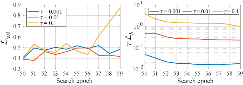
Figure 2: Search epoch vs. $\mathcal{L}_{\mathrm{val}}$ (left) and $\gamma\mathcal{L}_{\mathrm{\lambda}}$ (right). $\mathcal{L}_{\mathrm{val}}$ is plotted in linear scale, and $\gamma\mathcal{L}_{\mathrm{\lambda}}$ is plotted in logarithmic scale. It is clear that large $\gamma\mathcal{L}_{\mathrm{\lambda}}$ causes explosion in $\mathcal{L}_{\mathrm{val}}$.

Table 5: AdvRush compared to various standard adversarial training methods. $E_{\tiny\textrm{Warm}}$ and $E_{\tiny\textrm{Adv}}$ denote the number of epochs with and without the adversarial loss term, respectively.

Search	$E_{\tiny\textrm{Warm}}$	$E_{\tiny\textrm{Adv}}$	Clean	FGSM	PGD20	PGD100
FGSM	0	50	83.04%	56.30%	48.76%	48.47%
	0	60	82.82%	55.55%	48.41%	48.04%
	50	10	82.78%	54.17%	46.48%	46.03%
PGD	0	50	81.13%	53.59%	46.37%	45.95%
	0	60	81.87%	53.46%	46.22%	45.82%
	50	10	82.26%	54.87%	46.81%	46.63%
AdvRush			87.30%	60.87%	53.07%	52.80%

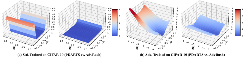
Figure 3: Loss landscape visualization for (a) standard-trained architectures and (b) adversarially-trained architectures. $\vec{n}$ and $\vec{r}$ denote perturbations in normal and random directions, respectively. The loss landscapes of AdvRush are visibly smoother than those of PDARTS.

Table 6: Architecture analysis. {M.P.; A.P.; S.; S.C.; D.C.} each refers to max pooling, average pooling, skip connect, seperable convolution, and dilated convolution. The width and the depth of an architecture are measured following Shu et al. [61], and N, R denote the normal and the reduction cell. Std. Tr. and Adv. Tr. refer to the HRS score of an architecture after standard and adversarial training.

Search	Arch	Params	# of Operations	Width	Depth	HRS ($\uparrow$)
			{M.P.; A.P.; S.; S.C.; D.C.}	{N, R}	{N, R}	Std. Tr.	Adv. Tr.
PDARTS		3.4M	{0; 1; 3; 9; 2}	{2.5c, 3c}	{4, 3}	69.92	64.10
AdvRush	Arch 0	4.2M	{0; 2; 4; 9; 1}	{4c; 3c}	{2, 3}	71.09	66.01
	Arch 1	4.2M	{0; 0; 5; 8; 3}	{4c, 3c}	{2, 3}	63.50	65.25
	Arch 2	4.2M	{0; 0; 4; 10; 2}	{3.5c, 3.5c}	{3, 3}	71.06	65.44
	Arch 3	3.8M	{0; 0; 6; 7; 3}	{4c, 3c}	{2, 3}	64.24	64.05
	Arch 4	3.7M	{0; 0; 5; 8; 3}	{4c, 4c}	{2, 2}	66.27	65.20
	Arch 5	2.9M	{4; 0; 3; 2; 7}	{4c, 3.5c}	{2, 3}	61.57	61.44
	Arch 6	3.0M	{4; 0; 3; 1; 8}	{4c, 3c}	{2, 3}	67.36	61.10
Supernet	Arch 7	2.3M	{5; 1; 6; 1; 3}	{4c, 3c}	{2, 3}	44.55	59.53
Adv. Tr.	Arch 8	2.3M	{1; 0; 4; 0; 11}	{3c, 3c}	{4, 3}	38.87	59.01
	Arch 9	2.1M	{1; 0; 6; 0; 9}	{3.5c, 3c}	{4, 3}	34.52	59.08
	Arch 10	2.3M	{0; 5; 7; 1; 3}	{4c, 2.5c}	{2, 3}	38.15	59.66

6.3 Examination of the Searched Architecture

To show that the AdvRush architecture in fact has a relatively smooth input loss landscape, we compare the input loss landscapes of the AdvRush and the PDARTS architectures after standard training and adversarial training in Figure 3. The loss landscapes are visualized using the same technique as utilized by Moosavi et al. [48]. Degrees of perturbation in input data for standard-trained and adversarially-trained architectures are set differently to account for the discrepancy in their sensitivity to perturbation. Independent of the training method, the input loss landscape of the AdvRush architecture is visibly smoother. The visualization results provide strong empirical support for AdvRush by demonstrating that the search result is aligned with our theoretical motivation.

We analyze the architectures used in our experiments to provide a meaningful insight into what makes an architecture robust. To begin with, we find that architectures that are based on the DARTS search space are generally more robust than hand-crafted architectures. The DARTS search space is inherently designed to yield an architecture with dense connectivity and complicated feature reuse. We believe that the complex wiring pattern of the DARTS search space allows derived architectures to be more robust than others, as observed by Guo et al. [24].

Furthermore, we compare the twelve architectures searched from the DARTS search space, through Harmonic Robustness Score (HRS) [14], a recently-introduced metric for measuring the trade-off between standard and robust accuracies. Details regarding the calculation of HRS can be found in the Appendix. In Table 6, we report the HRS of each architecture, along with the summary of its architectural details. Please refer to the Appendix for the visualization of each architecture. In general, robust architectures with high HRS have fewer parameter-free operations (i.e. pooling and skip connect) and more separable convolution operations. As a result, they tend to have more parameters than non-robust ones; this result coincides with the observations in Madry et al. [40] and Su et al. [63].

Also, the fact that Arch 5 & 6, in spite of having a fewer number of parameters, have comparable HRS to some of the larger architectures leads us to believe that the diversification of operations contributes to improving the robustness. The operational diversity is once again observed in PDARTS and Arch 0, both of which have high HRS. Lastly, no clear relationship between the width and the depth of an architecture and its robustness can be found, indicating that these two factors may have less influence over robustness.

7 Conclusion

In this work, AdvRush, a novel adversarial robustness-aware NAS algorithm, is proposed. The objective function of AdvRush is designed to prefer a candidate architecture with a smooth input loss landscape. The theoretical motivation behind our approach is validated by strong empirical results. Possible future works include the study of a robust neural architecture for multimodal datasets and expansion of the search space to include more diversified operations.

Appendices

A1 AdvRush Implementation Details

Following DARTS, the search space of AdvRush includes following operations:

• Zero Operation

• Skip Connect

• 3x3 Average Pooling

• 3x3 Max Pooling

• 3x3 Separable Conv

• 5x5 Separable Conv

• 3x3 Dilated Conv

• 5x5 Dilated Conv

The pseudo code is presented in Algorithm 1.

Input :  $E$ = total number of epochs for search

$E_{\mathrm{warmup}}$ = number of epochs to warm-up

$\gamma$ = regularization strength

Output :  $f^{*}_{A}(\cdot)$ = final architecture

1 Initialize $f_{\mathrm{super}}(\omega_{0},\alpha_{0})$

2 For $i$ = from $1$ to $E$:

3    If $i\leq E_{\mathrm{warmup}}$

4        Update $\omega_{i}$ using $\nabla_{\omega}\mathcal{L}_{\mathrm{train}}(\omega_{i-1},\alpha_{i-1})$ (SGD)

5        Update $\alpha_{i}$ using $\nabla_{\alpha}\mathcal{L}_{\mathrm{val}}(\omega_{i},\alpha_{i-1})$ (Adam)

6

7   Else

8        Update $\omega_{i}$ using $\nabla_{\omega}\mathcal{L}_{\mathrm{train}}(\omega_{i-1},\alpha_{i-1})$ (SGD)

9        Update $\alpha_{i}$ using $\nabla_{\alpha}[\mathcal{L}_{\mathrm{val}}(\omega_{i},\alpha_{i-1})+\gamma\mathcal{L}_{\lambda}]$ (Adam)

10

11   End

12End

13Derive $f^{*}_{A}(\cdot)$ through discretization rule of DARTS from $f_{\mathrm{super}}(\omega_{E},\alpha_{E})$

Algorithm 1 AdvRush (Search)

A2 Hyperparameters and Datasets

For adversarial training, a different set of hyperparameters for each dataset. Hyperparameter settings for the datasets used in our experiments are provided in Table A1. Details regarding the datasets are provided in Table A4.

Table A1: Details of hyperpameters used for adversarial training on different datasets. Learning rate is decayed by the factor of 0.1 at selected epochs. CIFAR refers to both CIFAR-10 and -100.

	CIFAR	SVHN	Tiny-ImageNet
Optimizer	SGD	SGD	SGD
Momentum	0.9	0.9	0.9
Weight decay	1e-4	1e-4	1e-4
Epochs	200	200	90
LR	0.1	0.01	0.1
LR decay	(100, 150)	(100, 150)	(30, 60)

A3 Difference in $\mathcal{L}_{\lambda}$

In Figure A1, we visualize how the difference in $\alpha$ update rule between DARTS and AdvRush affects the value of $\mathcal{L}_{\lambda}$. We use $\gamma$ of $0.01$ for AdvRush, and $\mathcal{L}_{\lambda}$ is introduced at the $50^{th}$ epoch. Notice that AdvRush experiences a steeper drop in $\mathcal{L}_{\lambda}$; this phenomenon implies that the final supernet of AdvRush is indeed smoother than that of DARTS. Since the only difference in the two compared search algorithms is the learning objective of $\alpha$, it is safe to assume that this extra smoothness is induced solely by the difference in $\alpha$.

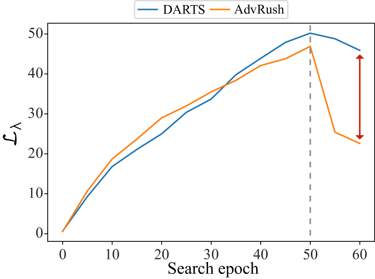
Figure A1: The difference in value of $\mathcal{L}_{\lambda}$ between DARTS and AdvRush. $\mathcal{L}_{\lambda}$ is introduced at Epoch $50$, noted in a gray dotted line. The red arrow points out the gap in $\mathcal{L}_{\lambda}$ between the two algorithms, caused by different $\alpha$ update rules.

A4 More Input Loss Landscapes

We provide additional input loss landscapes of other tested architectures after standard training (Figure A4) and adversarial training (Figure A5). All loss landscapes are drawn using the CIFAR-10 dataset. In both figures, $\vec{n}$ and $\vec{r}$ denote perturbations in normal and random directions, respectively. Degrees of perturbation in input data for standard trained and adversarially trained architectures are set differently to account for the discrepancy in their sensitivity to perturbation.

A5 Architecture Visualization

The architectures used for the analysis in Section 6.3 of the main text are visualized in Figure A2 and A3.

A6 HRS Calculation

HRS is calculated as follows:

$$HRS=\frac{2CR}{C+R}$$ (A1)

where C denotes the clean accuracy, and R denotes the robust accuracy. For standard-trained architectures, we use the robust accuracy under FGSM attack for R because the robust accuracy of standard-trained architectures under PGD attack reaches near-zero. For adversarially-trained architectures, we use the robust accuracy under PGD²⁰ attack for R. C, R, and HRS values for all architectures used in Section 6.3 of the main text can be found in Table A2.

A7 Extended Results on Other Datasets

In addition to the results in the main text, we conduct PGD attack with different number of iterations and evaluate the robust accuracy on CIFAR-100, SVHN, and Tiny-ImageNet. We use varying iterations from $7$ to $1000$. The results are visualized in Figure A6. AdvRush consistently outperforms other architectures, regardless of the strength of the adversary.

A8 Full Ablation Results

In Table A3, the full ablation analysis of AdvRush including the robust accuracies under AutoAttack is presented. No matter the value of $\gamma$ used, architectures searched with AdvRush achieve high robust accuracies under AutoAttack. Such results suggest that AdvRush does not require excessive tuning of $\gamma$ to search for a robust neural architecture.

Table A2: Effect of the change in the magnitude of $\gamma$. Baseline refers to the AdvRush with default $\gamma$ of 0.01. The best result in each column is in bold, and the second best result is underlined.

Arch	Std. Tr.			Adv. Tr.
	Clean	FGSM	HRS	Clean	PGD20	HRS
PDARTS	97.49%	54.51%	69.92	85.37%	51.32%	64.10
Arch 0	97.58%	55.91%	71.09	87.30%	53.07%	66.01
Arch 1	95.59%	47.54%	63.50	85.65%	52.70%	65.25
Arch 2	95.55%	56.57%	71.06	85.68%	52.93%	65.44
Arch 3	95.24%	48.46%	64.24	83.15%	53.42%	64.05
Arch 4	95.45%	50.75%	66.27	83.03%	53.67%	65.20
Arch 5	95.05%	45.53%	61.57	83.04%	48.76%	61.44
Arch 6	94.93%	52.20%	67.36	82.82%	48.41%	61.10
Arch 7	94.01%	29.19%	44.55	82.78%	46.48%	59.53
Arch 8	93.24%	24.55%	38.87	81.13%	46.37%	59.01
Arch 9	93.08%	21.19%	34.52	81.87%	46.22%	59.08
Arch 10	93.88%	23.94%	38.15	82.26%	46.81%	59.66

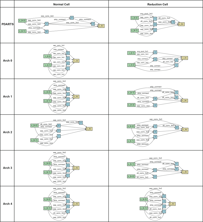
Figure A2: Architectures searched by PDARTS and AdvRush. A normal cell maintains the dimension of input feature maps, while a reduction cell reduces it. The entire neural network is constructed by stacking 18 normal cells and 2 reduction cells following the DARTS convention. The reduction cell is placed at the $1/3$ and $2/3$ points of the network.

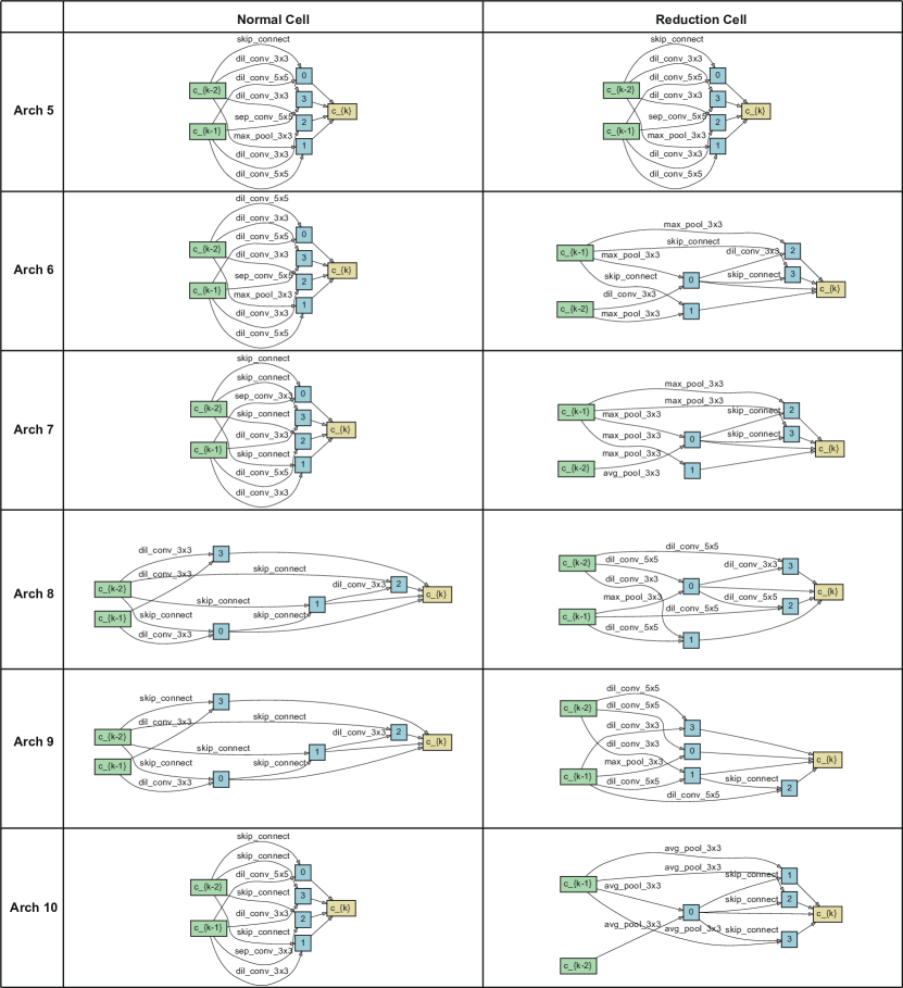
Figure A3: Architectures searched by adversarial training of the supernet. A normal cell maintains the dimension of input feature maps, while a reduction cell reduces it. The entire neural network is constructed by stacking 18 normal cells and 2 reduction cells following the DARTS convention. The reduction cell is placed at the $1/3$ and $2/3$ points of the network.

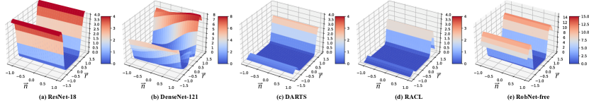
Figure A4: Input loss landscapes after standard training on CIFAR-10.

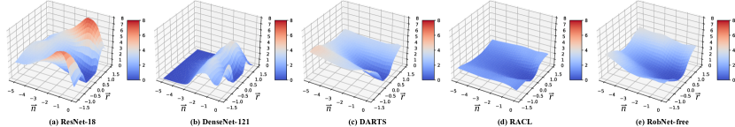
Figure A5: Input loss landscapes after adversarial training on CIFAR-10.

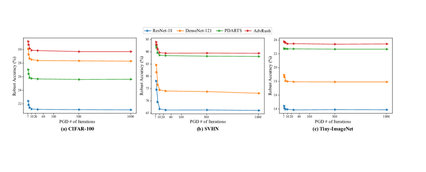
Figure A6: Robust accuracies on (a) CIFAR-100, (b) SVHN, and (c) Tiny-ImageNet under different iterations of PGD attack.

Table A3: Effect of the change in the magnitude of $\gamma$. Baseline refers to AdvRush with default $\gamma$ of 0.01. The best result in each column is in bold, and the second best result is underlined.

$\gamma$-value	Clean	FGSM	PGD20	PGD100	APGDCE	APGDT	FABT	Square	AA
0.001 (x 0.1)	85.65%	60.04%	52.70%	52.39%	51.39%	49.16%	49.13%	49.13%	49.13%
0.005 (x 0.5)	85.68%	60.31%	52.93%	52.61%	51.77%	49.63%	49.62%	49.62%	49.62%
0.01 (baseline)	87.30%	60.87%	53.07%	52.80%	50.05%	50.04%	50.04%	50.04%	50.04%
0.02 (x 2)	83.15%	59.34%	53.42%	53.19%	52.22%	49.60%	49.60%	49.60%	49.60%
0.1 (x 10)	83.03%	59.69%	53.67%	52.20%	51.22%	49.12%	49.11%	49.11%	49.11%

Table A4: Summary of datasets used for the experiments. CIFAR-10, CIFAR-100, and SVHN, which are available directly from torchvision, are split only into train and test sets by default.

Dataset	# of Train Data	# of Validation Data	# of Test Data	# of Classes	Image Size
CIFAR-10	50,000	-	10,000	10	$(32\times 32)$
CIFAR-100	50,000	-	10,000	100	$(32\times 32)$
SVHN	73,257	-	26,032	10	$(32\times 32)$
Tiny-ImageNet	100,000	5,000	5,000	200	$(64\times 64)$

References

- [1] Obfuscated gradients give a false sense of security: Circumventing defenses to adversarial examples. In Proceedings of the 35th International Conference on Machine Learning, pages 274–283, 2018.
- [2] Bowen Baker, Otkrist Gupta, Nikhil Naik, and Ramesh Raskar. Designing neural network architectures using reinforcement learning. In International Conference on Learning Representations, 2017.
- [3] Gabriel Bender, Pieter-Jan Kindermans, Barret Zoph, Vijay Vasudevan, and Quoc V. Le. Understanding and simplifying one-shot architecture search. In Proceedings of the 35th International Conference on Machine Learning, pages 550–559, 2018.
- [4] Wieland Brendel, Jonas Rauber, and Matthias Bethge. Decision-based adversarial attacks: Reliable attacks against black-box machine learning models. 2018.
- [5] Sébastien Bubeck, Yin Tat Lee, Eric Price, and Ilya Razenshteyn. Adversarial examples from computational constraints. In Proceedings of the 36th International Conference on Machine Learning, pages 831–840, 2019.
- [6] Nicholas Carlini and David Wagner. Towards evaluating the robustness of neural networks. In 2017 IEEE Symposium on Security and Privacy (S&P), pages 39–57. IEEE, 2017.
- [7] Pin-Yu Chen, Huan Zhang, Yash Sharma, Jinfeng Yi, and Cho-Jui Hsieh. Zoo: Zeroth order optimization based black-box attacks to deep neural networks without training substitute models. In Proceedings of the 10th ACM Workshop on Artificial Intelligence and Security, pages 15–26, 2017.
- [8] Xiangning Chen and Cho-Jui Hsieh. Stabilizing differentiable architecture search via perturbation-based regularization. 2020.
- [9] Xin Chen, Lingxi Xie, Jun Wu, and Qi Tian. Progressive differentiable architecture search: Bridging the depth gap between search and evaluation. In Proceedings of the IEEE International Conference on Computer Vision, pages 1294–1303, 2019.
- [10] Yukang Chen, Tong Yang, Xiangyu Zhang, Gaofeng Meng, Xinyu Xiao, and Jian Sun. Detnas: Backbone search for object detection. In Advances in Neural Information Processing Systems, pages 6638–6648, 2019.
- [11] Xiangxiang Chu, Tianbao Zhou, Bo Zhang, and Jixiang Li. Fair DARTS: Eliminating Unfair Advantages in Differentiable Architecture Search. In European Conference On Computer Vision, 2020.
- [12] Francesco Croce and Matthias Hein. Reliable evaluation of adversarial robustness with an ensemble of diverse parameter-free attacks. In Proceedings of the 37th International Conference on Machine Learning, 2020.
- [13] Jia Deng, Wei Dong, Richard Socher, Li-Jia Li, Kai Li, and Li Fei-Fei. Imagenet: A large-scale hierarchical image database. In 2009 IEEE conference on computer vision and pattern recognition, pages 248–255. Ieee, 2009.
- [14] Chaitanya Devaguptapu, Devansh Agarwal, Gaurav Mittal, and Vineeth N Balasubramanian. An empirical study on the robustness of nas based architectures. arXiv preprint arXiv:2007.08428, 2020.
- [15] Elvis Dohmatob. Generalized no free lunch theorem for adversarial robustness. In Proceedings of the 36th International Conference on Machine Learning, pages 1646–1654, 2019.
- [16] Minjing Dong, Yanxi Li, Yunhe Wang, and Chang Xu. Adversarially robust neural architectures. arXiv preprint arXiv:2009.00902, 2020.
- [17] Xuanyi Dong and Yi Yang. Searching for a robust neural architecture in four gpu hours. In Proceedings of the IEEE Conference on Computer Vision and Pattern Recognition, pages 1761–1770, 2019.
- [18] Alhussein Fawzi, Seyed-Mohsen Moosavi-Dezfooli, Pascal Frossard, and Stefano Soatto. Empirical study of the topology and geometry of deep networks. In Proceedings of the IEEE Conference on Computer Vision and Pattern Recognition, pages 3762–3770, 2018.
- [19] Timur Garipov, Pavel Izmailov, Dmitrii Podoprikhin, Dmitry P Vetrov, and Andrew G Wilson. Loss surfaces, mode connectivity, and fast ensembling of dnns. In Advances in Neural Information Processing Systems, pages 8789–8798, 2018.
- [20] Ian J Goodfellow, Jonathon Shlens, and Christian Szegedy. Explaining and harnessing adversarial examples. 2015.
- [21] Ian J Goodfellow, Oriol Vinyals, and Andrew M Saxe. Qualitatively characterizing neural network optimization problems. In International Conference on Learning Representations, 2015.
- [22] Chuan Guo, Jacob R Gardner, Yurong You, Andrew Gordon Wilson, and Kilian Q Weinberger. Simple black-box adversarial attacks. pages 2484–2493, 2019.
- [23] Jianyuan Guo, Kai Han, Yunhe Wang, Chao Zhang, Zhaohui Yang, Han Wu, Xinghao Chen, and Chang Xu. Hit-detector: Hierarchical trinity architecture search for object detection. In Proceedings of the IEEE/CVF Conference on Computer Vision and Pattern Recognition, pages 11405–11414, 2020.
- [24] Minghao Guo, Yuzhe Yang, Rui Xu, Ziwei Liu, and Dahua Lin. When nas meets robustness: In search of robust architectures against adversarial attacks. In Proceedings of the IEEE/CVF Conference on Computer Vision and Pattern Recognition, pages 631–640, 2020.
- [25] Kaiming He, Xiangyu Zhang, Shaoqing Ren, and Jian Sun. Deep residual learning for image recognition. In Proceedings of the IEEE conference on computer vision and pattern recognition, pages 770–778, 2016.
- [26] Gao Huang, Zhuang Liu, Laurens Van Der Maaten, and Kilian Q Weinberger. Densely connected convolutional networks. In Proceedings of the IEEE conference on computer vision and pattern recognition, pages 4700–4708, 2017.
- [27] Andrew Ilyas, Logan Engstrom, Anish Athalye, and Jessy Lin. Black-box adversarial attacks with limited queries and information. In Proceedings of the 35th International Conference on Machine Learning, pages 2137–2146, 2018.
- [28] Saumya Jetley, Nicholas Lord, and Philip Torr. With friends like these, who needs adversaries? In Advances in Neural Information Processing Systems, pages 10749–10759, 2018.
- [29] Chenhan Jiang, Hang Xu, Wei Zhang, Xiaodan Liang, and Zhenguo Li. Sp-nas: Serial-to-parallel backbone search for object detection. In Proceedings of the IEEE/CVF Conference on Computer Vision and Pattern Recognition, pages 11863–11872, 2020.
- [30] Yufan Jiang, Chi Hu, Tong Xiao, Chunliang Zhang, and Jingbo Zhu. Improved differentiable architecture search for language modeling and named entity recognition. In Proceedings of the 2019 Conference on Empirical Methods in Natural Language Processing and the 9th International Joint Conference on Natural Language Processing (EMNLP-IJCNLP), pages 3576–3581, 2019.
- [31] Harini Kannan, Alexey Kurakin, and Ian Goodfellow. Adversarial logit pairing. arXiv preprint arXiv:1803.06373, 2018.
- [32] Jihwan Kim, Jisung Wang, Sangki Kim, and Yeha Lee. Evolved speech-transformer: Applying neural architecture search to end-to-end automatic speech recognition. Proc. Interspeech 2020, pages 1788–1792, 2020.
- [33] Shashank Kotyan and Danilo Vasconcellos Vargas. Towards evolving robust neural architectures to defend from adversarial attacks. In Proceedings of the 2020 Genetic and Evolutionary Computation Conference Companion, pages 135–136, 2020.
- [34] Alex Krizhevsky, Geoffrey Hinton, et al. Learning multiple layers of features from tiny images. 2009.
- [35] Alexey Kurakin, Ian Goodfellow, and Samy Bengio. Adversarial examples in the physical world. 2017.
- [36] Saehyung Lee, Hyungyu Lee, and Sungroh Yoon. Adversarial vertex mixup: Toward better adversarially robust generalization. In Proceedings of the IEEE/CVF Conference on Computer Vision and Pattern Recognition, pages 272–281, 2020.
- [37] Hao Li, Zheng Xu, Gavin Taylor, Christoph Studer, and Tom Goldstein. Visualizing the loss landscape of neural nets. In Advances in Neural Information Processing Systems, pages 6389–6399, 2018.
- [38] Chenxi Liu, Liang-Chieh Chen, Florian Schroff, Hartwig Adam, Wei Hua, Alan L Yuille, and Li Fei-Fei. Auto-deeplab: Hierarchical neural architecture search for semantic image segmentation. In Proceedings of the IEEE/CVF Conference on Computer Vision and Pattern Recognition, pages 82–92, 2019.
- [39] Hanxiao Liu, Karen Simonyan, and Yiming Yang. Darts: Differentiable architecture search. In International Conference on Learning Representations, 2019.
- [40] Aleksander Madry, Aleksandar Makelov, Ludwig Schmidt, Dimitris Tsipras, and Adrian Vladu. Towards deep learning models resistant to adversarial attacks. 2018.
- [41] Dongyu Meng and Hao Chen. Magnet: a two-pronged defense against adversarial examples. In Proceedings of the 2017 ACM SIGSAC conference on computer and communications security, pages 135–147, 2017.
- [42] Jan Hendrik Metzen, Tim Genewein, Volker Fischer, and Bastian Bischoff. On detecting adversarial perturbations. In International Conference on Learning Representations, 2017.
- [43] Takeru Miyato, Shin-ichi Maeda, Masanori Koyama, and Shin Ishii. Virtual adversarial training: a regularization method for supervised and semi-supervised learning. volume 41, pages 1979–1993. IEEE, 2018.
- [44] Tong Mo, Yakun Yu, Mohammad Salameh, Di Niu, and Shangling Jui. Neural architecture search for keyword spotting. arXiv preprint arXiv:2009.00165, 2020.
- [45] Seungyong Moon, Gaon An, and Hyun Oh Song. Parsimonious black-box adversarial attacks via efficient combinatorial optimization. In International Conference on Machine Learning, pages 4636–4645, 2019.
- [46] Seyed-Mohsen Moosavi-Dezfooli, Alhussein Fawzi, Omar Fawzi, and Pascal Frossard. Universal adversarial perturbations. In Proceedings of the IEEE/CVF Conference on Computer Vision and Pattern Recognition, pages 1765–1773, 2017.
- [47] Seyed-Mohsen Moosavi-Dezfooli, Alhussein Fawzi, and Pascal Frossard. Deepfool: a simple and accurate method to fool deep neural networks. In Proceedings of the IEEE/CVF Conference on Computer Vision and Pattern Recognition, pages 2574–2582, 2016.
- [48] Seyed-Mohsen Moosavi-Dezfooli, Alhussein Fawzi, Jonathan Uesato, and Pascal Frossard. Robustness via curvature regularization, and vice versa. In Proceedings of the IEEE/CVF Conference on Computer Vision and Pattern Recognition, pages 9078–9086, 2019.
- [49] Vladimir Nekrasov, Hao Chen, Chunhua Shen, and Ian Reid. Fast neural architecture search of compact semantic segmentation models via auxiliary cells. In Proceedings of the IEEE Conference on computer vision and pattern recognition, pages 9126–9135, 2019.
- [50] Yuval Netzer, Tao Wang, Adam Coates, Alessandro Bissacco, Bo Wu, and Andrew Y Ng. Reading digits in natural images with unsupervised feature learning. 2011.
- [51] Nicolas Papernot and Patrick McDaniel. Extending defensive distillation. arXiv preprint arXiv:1705.05264, 2017.
- [52] Nicolas Papernot, Patrick McDaniel, Ian Goodfellow, Somesh Jha, Z Berkay Celik, and Ananthram Swami. Practical black-box attacks against machine learning. In Proceedings of the 2017 ACM on Asia Conference on Computer and Communications Security, pages 506–519, 2017.
- [53] Nicolas Papernot, Patrick McDaniel, Somesh Jha, Matt Fredrikson, Z Berkay Celik, and Ananthram Swami. The limitations of deep learning in adversarial settings. In 2016 IEEE European Symposium on Security and Privacy (EuroS&P), pages 372–387. IEEE, 2016.
- [54] Hieu Pham, Melody Y. Guan, Barret Zoph, Quoc V. Le, and Jeff Dean. Efficient neural architecture search via parameter sharing. In Proceedings of the 35th International Conference on Machine Learning, pages 4095–4104, 2018.
- [55] Chongli Qin, James Martens, Sven Gowal, Dilip Krishnan, Krishnamurthy Dvijotham, Alhussein Fawzi, Soham De, Robert Stanforth, and Pushmeet Kohli. Adversarial robustness through local linearization. In Advances in Neural Information Processing Systems, pages 13847–13856, 2019.
- [56] Xiaoyang Qu, Jianzong Wang, and Jing Xiao. Evolutionary algorithm enhanced neural architecture search for text-independent speaker verification. Proc. Interspeech 2020, pages 961–965, 2020.
- [57] Esteban Real, Alok Aggarwal, Yanping Huang, and Quoc V Le. Regularized evolution for image classifier architecture search. In Proceedings of the AAAI Conference on Artificial Intelligence, volume 33, pages 4780–4789, 2019.
- [58] Esteban Real, Sherry Moore, Andrew Selle, Saurabh Saxena, Yutaka Leon Suematsu, Jie Tan, Quoc V Le, and Alexey Kurakin. Large-scale evolution of image classifiers. In Proceedings of the 34th International Conference on Machine Learning-Volume 70, pages 2902–2911. JMLR. org, 2017.
- [59] Andrew Slavin Ross and Finale Doshi-Velez. Improving the adversarial robustness and interpretability of deep neural networks by regularizing their input gradients. In Association for the Advancement of Artificial Intelligence, 2018.
- [60] Pouya Samangouei, Maya Kabkab, and Rama Chellappa. Defense-gan: Protecting classifiers against adversarial attacks using generative models. In International Conference on Learning Representations, 2018.
- [61] Yao Shu, Wei Wang, and Shaofeng Cai. Understanding architectures learnt by cell-based neural architecture search. In International Conference on Learning Representations, 2019.
- [62] Yang Song, Taesup Kim, Sebastian Nowozin, Stefano Ermon, and Nate Kushman. Pixeldefend: Leveraging generative models to understand and defend against adversarial examples. In International Conference on Learning Representations, 2018.
- [63] Dong Su, Huan Zhang, Hongge Chen, Jinfeng Yi, Pin-Yu Chen, and Yupeng Gao. Is robustness the cost of accuracy?–a comprehensive study on the robustness of 18 deep image classification models. In Proceedings of the European Conference on Computer Vision (ECCV), pages 631–648, 2018.
- [64] Jiawei Su, Danilo Vasconcellos Vargas, and Kouichi Sakurai. One pixel attack for fooling deep neural networks. volume 23, pages 828–841. IEEE, 2019.
- [65] Christian Szegedy, Wojciech Zaremba, Ilya Sutskever, Joan Bruna, Dumitru Erhan, Ian Goodfellow, and Rob Fergus. Intriguing properties of neural networks. arXiv preprint arXiv:1312.6199, 2013.
- [66] Mingxing Tan, Ruoming Pang, and Quoc V Le. Efficientdet: Scalable and efficient object detection. In Proceedings of the IEEE/CVF Conference on Computer Vision and Pattern Recognition, pages 10781–10790, 2020.
- [67] Dimitris Tsipras, Shibani Santurkar, Logan Engstrom, Alexander Turner, and Aleksander Madry. Robustness may be at odds with accuracy. In International Conference on Learning Representations, 2019.
- [68] Chaowei Xiao, Bo Li, Jun-Yan Zhu, Warren He, Mingyan Liu, and Dawn Song. Generating adversarial examples with adversarial networks. arXiv preprint arXiv:1801.02610, 2018.
- [69] Cihang Xie, Yuxin Wu, Laurens van der Maaten, Alan L Yuille, and Kaiming He. Feature denoising for improving adversarial robustness. In Proceedings of the IEEE/CVF Conference on Computer Vision and Pattern Recognition, pages 501–509, 2019.
- [70] Sirui Xie, Hehui Zheng, Chunxiao Liu, and Liang Lin. Snas: stochastic neural architecture search. In International Conference on Learning Representations, 2018.
- [71] Weilin Xu, David Evans, and Yanjun Qi. Feature squeezing: Detecting adversarial examples in deep neural networks. In Network and Distributed Systems Security Symposium, 2018.
- [72] Yuhui Xu, Lingxi Xie, Xiaopeng Zhang, Xin Chen, Guo-Jun Qi, Qi Tian, and Hongkai Xiong. Pc-darts: Partial channel connections for memory-efficient architecture search. In International Conference on Learning Representations, 2019.
- [73] Fuxun Yu, Zhuwei Qin, Chenchen Liu, Liang Zhao, Yanzhi Wang, and Xiang Chen. Interpreting and evaluating neural network robustness. In Proceedings of the 28th International Joint Conference on Artificial Intelligence, pages 4199–4205. AAAI Press, 2019.
- [74] Haichao Zhang and Jianyu Wang. Defense against adversarial attacks using feature scattering-based adversarial training. In Advances in Neural Information Processing Systems, pages 1831–1841, 2019.
- [75] Hongyang Zhang, Yaodong Yu, Jiantao Jiao, Eric P Xing, Laurent El Ghaoui, and Michael I Jordan. Theoretically principled trade-off between robustness and accuracy. In Proceedings of the 36th International Conference on Machine Learning, pages 7472–7482, 2019.
- [76] Miao Zhang, Huiqi Li, Shirui Pan, Xiaojun Chang, and Steven Su. Overcoming multi-model forgetting in one-shot nas with diversity maximization. In Proceedings of the IEEE/CVF Conference on Computer Vision and Pattern Recognition, pages 7809–7818, 2020.
- [77] Yiheng Zhang, Zhaofan Qiu, Jingen Liu, Ting Yao, Dong Liu, and Tao Mei. Customizable architecture search for semantic segmentation. In Proceedings of the IEEE Conference on Computer Vision and Pattern Recognition, pages 11641–11650, 2019.
- [78] Pu Zhao, Pin-Yu Chen, Payel Das, Karthikeyan Natesan Ramamurthy, and Xue Lin. Bridging mode connectivity in loss landscapes and adversarial robustness. In International Conference on Learning Representations, 2020.
- [79] Barret Zoph and Quoc V. Le. Neural architecture search with reinforcement learning. In International Conference on Learning Representations, 2017.
- [80] Barret Zoph, Vijay Vasudevan, Jonathon Shlens, and Quoc V Le. Learning transferable architectures for scalable image recognition. In Proceedings of the IEEE conference on Computer Vision and Pattern Recognition, pages 8697–8710, 2018.