The Electric Vehicle Routing Problem with Nonlinear Charging Functions

Yijing Liang School of Management and Engineering,Nanjing University,Nanjing 210093, P.R. China, liangyj@smail.nju.edu.cn Said Dabia Department of Operations Analytics, Vrije Universiteit Amsterdam, 1081 HV Amsterdam, Netherlands, s.dabia@vu.nl Zhixing Luo School of Management and Engineering,Nanjing University,Nanjing 210093, P.R. China, luozx.hkphd@gmail.com

This paper outlines an exact and a heuristic algorithm for the electric vehicle routing problem with a nonlinear charging function (E-VRP-NL) introduced by Montoya et al. (2017). The E-VRP-NL captures several realistic features of electric vehicles including the battery limited driving range and nonlinear charging process at the charging stations. We formulate this problem as a set-partitioning and solve it using a column generation based algorithm. The resulting pricing problem of the column generation is a complicated problem as, next to the usual operational constraints e.g. time windows and vehicle capacity, electric vehicle related features are also considered. In particular, the nonlinear nature of the battery charging process requires the incorporation of a set of sophisticated recursive functions in the pricing algorithm. We show how these recursive functions allow for the simultaneous evaluation of the routing and charging decisions. Moreover, we illustrate how they can efficiently be embedded in the pricing algorithm. The column generation algorithm is integrated in a branch and bound algorithm and cutting planes are added resulting in a branch-and-price-and-cut algorithm for the E-VRP-NL. Next to the exact algorithm, we also develop a tabu search based heuristic to solve the problem quickly. To prove the efficiency of the proposed algorithms, their performance is tested on benchmark instances from the literature. Our exact algorithm can optimally solve instances with up to 40 customers, including several instances previously unsolved to optimality. The tabu search heuristic proves to be superior to state-of-the-art heuristics in the literature both on solution quality and computation times.

electric vehicle routing problem; nonlinear charging functions; branch-and-price; branch-and-price-and-cut; tabu search

1 Introduction

Worldwide concerns regarding climate change, air pollution, sustainability and living quality are growing considerably. The transport sector is one of the biggest contributors to the negative effects on the environment in the form of greenhouse gas (GHG) emissions, noise and congestion. As such, the reduction of the greenhouse gas (GHG) emission has become a challenge that must be tackled urgently. In 2017, the transportation sector counted for 28.9% of the total GHG emissions in the United States (United States Environmental Protection Agency 2017). In China, the Average Carbon Emission Intensity of the transportation sector is the highest, e.g 118 times larger than the financial sector (Ge 2013). To face this threatening trend, increasingly stringent environmental regulations and targets have been established in many countries. For example, the amount of carbon monoxide allowed to be emitted has been decreased by 50% in China’s Emission Standard (Stage vi@) (MEE 2017). As a result, the transport sector has undergone tremendous changes in terms of new practices and technology. Electric Vehicles (EVs) are a potential instrument for confronting these environmental challenges and achieving the targets set by governmental regulations. However, EVs suffer from several technical performance weaknesses, especially the limited battery driving range and the long charging times. Yet, due to the rapid technological developments regarding battery driving range, the decreasing battery prices, and the long-term rising fuel costs, several leading transportation companies like Fedex, DHL, UPS and DPD have been implementing EVs for their last-mile delivery operations. This trend is confirmed by the Edison Electric Institute (2019), that reported the sales of EVs increased by 79%, 78% and 34% in the U.S., China and Europe, respectively, in 2018.

To boost the wider uptake of EVs, it is essential to minimize the operating cost throughout their lifetime. To further drive down their total cost of ownership, improving and developing novel planning and routing tools that take the specifics of EVs into account is indispensable. The routing of EVs concerns the determination of a set of routes with least cost that comply with both the operational constraints and EVs features. This problem is known in the literature under the name the Electric Vehicle Routing Problems (E-VRPs)(see e.g. Schneider et al. (2014)) and fall under the more general family of Green Vehicle Routing Problems (G-VRPs) characterized by including environmental features (see e.g. Erdoğan and Miller-Hooks (2012)). Next to E-VRPs, another stream of research considers the cost of emissions directly in the objective function, e.g. the pollution routing problems (Bektaş and Laporte 2011, Dabia et al. 2017) and the emission VRPs (Figliozzi 2010).

It is not straightforward to estimate the battery charging time accurately as it depends on various factors such as the State of Charge (SoC) and the charging speed. To overcome this issue, simplistic battery charging functions are assumed in the literature to allow tractable models. In particular, in most research papers dealing with E-VRPs, the charging functions are assumed to be linear or even constant in the SoC. Some studies assume batteries are recharged to their maximum capacity (Schneider et al. 2014, Afroditi et al. 2014, Preis et al. 2014, Goeke and Schneider 2015, Hiermann et al. 2016). Clearly, partial charging can prevent unnecessary charging times and hence reduce routing costs as pointed out by Keskin and Çatay (2015). Consequently, other studies consider a battery partial charging policy in which the amount of energy charged is a decision variable (see e.g. Keskin and Çatay (2015), Bruglieri et al. (2015), Desaulniers et al. (2016), Montoya et al. (2015), Schiffer and Walther (2017), Montoya et al. (2017)). On the nature of the battery charging time, Pelletier et al. (2017) illustrate that the charging process comprises two stages. During the first stage, the SoC increases linearly with the charging time. In the second stage, the speed of charging decreases and the SoC increases concavely with the charging time to avoid overcharge. Hence the charging process is governed by a nonlinear relationship between the SoC and the charging time. Dealing with such a nonlinear relationship in planning algorithms for E-VRPs is a challenging task.

Existing methods from the scientific literature cannot cope with the additional complexities stemming from nonlinear battery charging time functions. As explained by Montoya et al. (2017), real charging functions are governed by differential equations and incorporating them into E-VRP models will drastically increase the computational difficulty. With this research, we aim to develop an exact method and a heuristic that capture realistic battery charging time functions, yet still remain tractable. We propose approximating the battery charging time function by means of a piecewise linear function. We must note, as pointed out by Montoya et al. (2015), that approximating nonlinear battery charging time functions may on one hand underestimate charging times leading to infeasible routes. On the other hand, conservative transport plans may be generated if charging times are overestimated leading to higher routing costs. Several researchers have adopted piecewise linear approximations of the battery charging time functions. However, all developed solution methods so far are heuristic based (Montoya et al. 2015, 2017, Froger et al. 2017, 2019). We are aware of one paper that directly employs nonlinear charging functions (Lee 2020).

Formally, we study the Electric Vehicle Routing Problem with Nonlinear Charging functions (E-VRP-NL). The nonlinear charging process at a charging station (CS) is approximated using a piecewise linear function. A homogeneous fleet of EVs is available to fulfil the demand of a set of geographically dispersed customers. Each EV is characterized by a limited battery driving range and storage capacity for loading cargo. For charging the batteries, a set of heterogeneous CSs with different charging functions is available. The E-VRP-NL concerns the determination of a set of routes with the least total duration where each customer is visited exactly once. Moreover, routes are required to start and end at a depot, the total quantity served along a route does not exceed the vehicle’s storage capacity and the battery driving range must be respected. Furthermore, the duration of each route must not exceed a limited allowed time. The route duration includes travel, waiting, service and charging time. We present here, to the best of our knowledge, the first exact approach for the E-VRP-NL based on a branch-and-price-and-cut (BPC) algorithm that incorporates several new features. More precisely, we developed specialized pricing procedures that efficiently handle the piecewise battery charging time functions. Moreover, new dominance procedures are introduced exploiting the problem’s structure. Next, a tabu search based heuristic is also developed to solve larger instances quickly.

In summary, the scientific contributions of our paper are as follows. First, we derive exact and heuristic algorithms that efficiently deal with sophisticated recursive functions that are needed to capture a more realistic battery charging process for EVs. Another benefit of this approach is that the routing and charging decisions are performed simultaneously. Second, we propose a BPC algorithm that can solve the E-VRP-NL to optimality for the first time. A tailored label-setting algorithm involving stronger dominance rules enabling a set of labels to dominate one label is proposed for the pricing problem of the underlying column generation algorithm. Third, we develop a tabu search algorithm to solve larger instances of the problem quickly. Through extensive computational experiments, we show that our exact algorithm substantially outperforms MILP solvers and other algorithms in the literature in both the number of instances solved optimally and computational time. The tabu search heuristic has also proven to be superior to state-of-the-art heuristics in the literature both on solution quality and computation time.

The reminder of the paper is organized as follows. In section 2, we review the literature related to the E-VRP-NL. Section 3 presents the description of the problem along with the set-partitioning formulation. Sections 4 and 5 ouline the details of the exact algorithms, and section 6 describes the tabu search heuristic. The computational results are presented in section 7. Finally, section 8 concludes the paper.

2 Literature Review

In this section, we review the literature related to the E-VRP-NL and other close problems in the family of the Green Vehicle Routing Problems (G-VRP). In particular, we review literature on routing alternative fuel-powered vehicles (AFVs), the Electric Vehicle Routing Problem (E-VRP), the Electric Location Routing Problem (E-LRP) and the Two-Echelon Electric Vehicle Routing Problem (2E-E-VRP).

Early work on the routing of EVs lies in the field of Green Vehicle Routing Problem (G-VRP) first introduced by Erdoğan and Miller-Hooks (2012). The family of G-VRPs takes sustainability measures into consideration either by including sustainability related costs in the objective function (Bektaş and Laporte 2011, Dabia et al. 2017) or by adopting environmentally friendly vehicles powered by alternative energy resources such as biodiesel, electricity and hydrogen (Erdoğan and Miller-Hooks 2012, Schneider et al. 2014). Unlike Erdoğan and Miller-Hooks (2012) where the refuelling time of AFVs is set to be fixed and the fully refuelling policy is employed, other studies allow partial recharges, and the charging amount is regarded as a decision variable. In Felipe et al. (2014), the G-VRP with partial recharges is studied where, at each CS, multiple charging technologies are available and the objective is to determine the charging amount and charging technology for each EV in order to minimize recharging cost. A heuristic integrating a greedy construction and a local search procedure into a simulated annealing framework is developed to solve the problem.
Another stream of research considers, next to partial charging, a mixed fleet where both conventional vehicles and AFVs are used for delivery. In Sassi et al. (2014), next to the mixed fleet, the charging cost is assumed to be time-dependent. The objective is to minimize the number of vehicles as well as the total cost including both travel and charging cost. Macrina et al. (2019a) further extend the problem by incorporating energy consumption functions that depend on various factors including speed, acceleration, deceleration, load and gradients into the optimization models. They develop a hybrid large neighborhood search (HLNS) algorithm. In Macrina et al. (2019b) energy consumption for conventional vehicles is calculated as the product of the distance traveled and emission factors which depend on cargo load, and is handled as constraints in the proposed model. An iterative local search is used as a solution method. To solve the G-VRP exactly, Andelmin and Bartolini (2017) propose an algorithm based on a multigraph where nodes represent customers, and arcs represent non-dominated paths. The results show that the algorithm can optimally solve instances with up to 110 customers. Related research dealing with fleet composition resulted in several papers (e.g. Hiermann et al. (2016), Sassi et al. (2015), Goeke and Schneider (2015), Hiermann et al. (2019)).

The EVs differ substantially from the AFVs in that they require longer charging times and their driving range is susceptible to several factors such as temperature, speed, acceleration, load, and road angle (Pelletier et al. 2016). Consequently, the routing optimization of EVs requires planning algorithms that are substantially different from these used for routing AFVs. Lin et al. (2016) study an E-VRP where the cost of travelling and energy consumption is minimized. The energy consumption is assumed to depend on the vehicle load, road angle and rolling resistance. Successful researches incorporating comprehensive energy consumption functions into routing models for EVs are performed by e.g. Zhang et al. (2018) and Basso et al. (2019). Schneider et al. (2014) introduce the electric vehicle routing problem with time windows and recharging stations (E-VRPTW). The recharging time is assumed to be linear in the SoC and the objective is to minimize the number of employed EVs and the total traveled distance. The problem is solved by a hybrid heuristic which incorporates a variable neighborhood search algorithm in a tabu search framework. In another study, Afroditi et al. (2014) consider the E-VRPTW where the charging time is set to be constant at each CS. Both researches require the battery of an EV is fully charged after paying a visit to a CS. Keskin and Çatay (2016) relax this assumption and allow for battery partial recharges in the E-VRPTW. They solve the problem with an Adaptive Large Neighborhood Search (ALNS) algorithm. Keskin and Çatay (2018) further extend the problem by considering different charging rates, i.e. normal, fast and super-fast. In their ALNS algorithm, the incumbent routes are improved by a destroy and repair process followed by an enhancement procedure based on a MILP model that optimizes the charging decisions. Bruglieri et al. (2015) propose a MILP formulation for the E-VRPTW also assuming battery partial recharging. The model aims to minimize the total cost consisting of travel, waiting and recharging time plus the number of the employed EVs. Moreover, a Variable Neighborhood Search Branching (VNSB) is developed to enable the solution of the problem in reasonable computational times. The only exact approach we are aware of for the E-VRPTW is attributed to Desaulniers et al. (2016) who propose a BPC algorithm able to solve four variants of the problem, i.e. single vs. multiple recharges and full vs. partial recharges.

Recent research is moving towards more realistic models. In particular, a few papers consider nonlinear charging functions in the E-VRPs resulting in the E-VRP-NL. Montoya et al. (2015, 2017) propose a node-based model for the E-VRP-NL in which the time and SoC at each node are tracked by a set of node-indexed variables. Their computational results prove the benefit of including the nonlinear charging time and partial recharges. A two-phase approach is developed: a hybrid heuristic based on an iterated local search is proposed for constructing routes, followed by a greedy procedure or a MILP to optimize battery charge-related decisions when routes are fixed. Froger et al. (2019) further improve the route construction phase by introducing two enhanced formulations, i.e. an arc-based model and a path-based model. The nodes representing the CSs are replicated in the arc-based model to accommodate for possible multiple visits. However, the number of copies is difficult to set as excessive copies imply longer solving times, while insufficient copies may lead to an infeasible problem. To avoid replicating the CS nodes, the path-based model incorporates the concept of CS path which denotes the sequence of visited CSs lying between two nodes (customer or depot). A label-correcting algorithm along with dominance rules are provided to generate non-dominated CS paths. Results show that the MILP solver can solve more instances based on the path-based model. However, the second phase where the charging is decided on remains time consuming, making route evaluation procedures computationally exhaustive. Lee (2020) develop an exact method for a variant of the E-VRP-NL in which: (i) a nonlinear charging function is assumed; (ii) only a single vehicle is assigned to serve all customers; (iii) neither storage capacity nor time window constraints are considered, and (iv) the depot is also a CS and can be visited several times. A branch-and-price algorithm is developed based on an extended CS network. A route is segmented into several no-charge segments starting from and ending at the depot or CSs. A label-setting algorithm generates no-charge segments with negative reduced cost and hence avoid handling the complicated nonlinear charging functions. The master problem finds a set of segments to construct a route with minimum travel and charging time. Additional constraints are needed in the master problem to combine no-charge segments into a feasible route. Pelletier et al. (2018) solve the problem of deciding on charging schedules for a fleet of EVs over multiple days given routes are fixed. In the model, realistic charging functions are approximated using piecewise linear functions. In Koç et al. (2019) the electric vehicle routing problem with piecewise linear charging functions is considered. Moreover, the CSs are allowed to be shared among different companies.

Other EV related features that attracted the attention of researchers are related to CSs. On the one hand, the CSs capacity is assumed to be limited and is expressed in the maximum number of EVs that can be charged simultaneously at a CS. Froger et al. (2018) consider a limited CS capacity in the E-VRP-NL and solve the problem using a route-first assemble-second metaheuristic. An extension of this problem is studied by Sweda et al. (2017) where the availability of CSs at any point in time is probabilistic. Several algorithms are introduced for finding an optimal a priori routing and recharging policy followed by solution approaches to an adaptive problem that build upon the a priori policy. On the other hand, another stream of research has focused on the Location Routing Problem that includes decisions related to the location of CSs into E-VRPs. Yang and Sun (2015) augment the problem by allowing battery swap at CSs. The objective is to minimize travel cost of the EVs and the construction cost of CSs. Hof et al. (2017) propose an adaptive variable neighborhood search algorithm (AVNS) that outperforms Yang and Sun (2015) in both computation time and solution quality. Arslan and Karaşan (2016) use a benders decomposition approach to decide on the location of the CSs for multiple types of plug-in hybrid EVs with different ranges and that can be powered by either gasoline or electricity. Schiffer and Walther (2017) study a location routing problem with time windows and a partial recharges policy.

Finally, Breunig et al. (2019) explore the Two-Echelon Electric Vehicle Routing Problem (2E-E-VRP) and develop an LNS-based algorithm and an exact algorithm to solve it. Conventional vehicles are employed in the first echelon while EVs are used for the second echelon. The objective is to find the set of routes with the least cost for both echelons in order to transport goods from the depot to customers through satellites. In opposite to Breunig et al. (2019), Jie et al. (2019) consider a 2E-E-VRP with battery swapping stations and heterogeneous EVs in both echelons. The problem is solved by a hybrid algorithm integrating a column generation algorithm and an adaptive large neighborhood search (ALNS).

3 Problem Description and Formulation

Let $G=(V,A)$ be a complete digraph where $V=\{0,1,\ldots,n,n+1,\ldots,n+m\}$ is the node set and $A=\{(i,j)~{}|~{}i,j\in V,i\neq j\}$ is the arc set. Node $0$ represents the depot, the node subset $N=\{1,\ldots,n\}$ corresponds to $n$ customers, and the node subset $R=\{n+1,\ldots,n+m\}$ corresponds to $m$ recharging stations. Each customer $i\in N$ requires a service time $s_{i}$ and has a demand $q_{i}$. Furthermore, traversing arc $(i,j)\in A$ requires a travel time $t_{i,j}$ and an amount $b_{i,j}$ of energy. The travel time matrix is supposed to satisfy the triangle inequality. We assume a limited fleet of $K$ homogenous electric vehicles is available with a limited storage capacity $Q$ and a limited battery driving range $B$. Each vehicle is required to complete its route within a time limit $T$. We denote $[e_{0},l_{0}]=[0,T]$ the depot’s time window, and $[e_{i},l_{i}]=[t_{0,i},T-s_{i}-t_{i,0}]$ the time window of customer $i\in N$. Similar to Montoya et al. (2017), the charging process consists of two stages. In the first stage the battery is charged at a constant rate, while in the second stage the SoC increases concavely with the charging time. This nonlinear charging process is approximated by a piecewise linear function. We assume heterogeneous CSs, where each CS $i\in R$ is characterized by a different non-decreasing piecewise linear charging function $r_{i}(t)$. Figure 1 illustrates an example of a nonlinear charging function approximated by a piecewise function.

Figure 1: A charging function approximated using a piecewise linear function (Montoya et al. 2017)

Our objective is to determine the set of routes with the least total duration such that: 1) the quantity moved along a route does not exceed the EV’s storage capacity $Q$; 2) the battery level of the EV along a route must remain between $0$ and $B$; 3) every customer can only be served by one EV during its corresponding time window and 4) the duration of each trip must not exceed the time limit $T$. We note that a route duration comprises travel, waiting, service and charging times.

3.1 The master problem

To derive the set partitioning formulation for the E-VRP-NL, we define $\Omega$ as the set of feasible routes. A route is feasible if it satisfies time window, storage capacity, battery driving range and duration time limit constraints. We let $c_{p}$ denote the duration (i.e. cost) of the route $p\in\Omega$ . For each route $p\in\Omega$, we let $\alpha_{i,p}$ be a constant that counts the number of times node $i$ is visited by the route $p$. Furthermore, $\theta_{p}$ is a binary variable that takes the value 1 if and only if the route $p$ is included in the solution, the E-VRP-NL is formulated as the following set-partitioning problem:

$$\min\sum_{p\in\Omega}c_{p}\theta_{p},$$ (1)

s.t. $$\sum_{p\in\Omega}\theta_{p}\leq K,$$ (2)

$$\sum_{p\in\Omega}\alpha_{i,p}\theta_{p}=1,\quad\forall i\in N,$$ (3)

$$\theta_{p}\in\{0,1\},\quad\forall p\in\Omega.$$ (4)

The objective function (1) minimizes the total duration of the chosen routes. The number of employed vehicles is limited to $K$ in constraint (2), and constraints (3) guarantee that each node is visited exactly once. We use column generation to solve the linear programming (LP) relaxation of problem (1)-(4): starting with a small subset $\Omega^{\prime}=\Omega$ of variables, we generate additional variables for the master problem (the LP relaxation of (1)-(4)) by solving a pricing problem that searches for variables with negative reduced cost. The column generation procedure terminates when no new variables with negative reduced cost are found.

3.2 The pricing problem

The pricing problem for the E-VRP-NL is an extension of the elementary shortest path problem with resource constraints (ESPPRC). Let $\mu_{0}$ and $\mu_{i}$ $(i\in N)$ be the dual values of constraints (2) and (3), respectively. The objective function of the pricing problem is formulated as follows:

$$\min_{p\in\Omega}c_{p}-\sum_{i\in N}\alpha_{i,p}\mu_{i}-\mu_{0},$$ (5)

The objective function (5) seeks the route with the least reduced cost. If the objective value of the pricing problem is nonnegative, the current solution of the master problem is optimal. We solve the pricing problem by a bounded bi-directional label-setting algorithm. For some good papers applying a (bi-directional) label-setting algorithm, we refer the reader to Feillet et al. (2004), Costa et al. (2019), Righini and Salani (2006) and Boland et al. (2006). The bounded bi-directional search split the extension process into a forward extension which extends from the (start) depot to its successors and a backward extension which extends from the (end) depot to its predecessors. The forward and backward labels are merged to construct complete routes. The basic operation in the label-setting algorithm is the extension of an existing label along an arc to generate a new label. These label extensions involve recursive functions that calculate the states of the newly generated labels. These recursive functions are more complicated than the ones used for the standard ESPPRC and play a key role in our algorithm. Next, we describe in more details the label-setting algorithm for both the forward and backward search including the specialized recursive functions.

4 The Pricing Algorithm

In this paper, we propose an exact algorithm based on column generation to solve the E-VRP-NL. In this section, we focus on the pricing algorithm which is a label-setting algorithm used to solve the pricing problem. In particular, we introduce the specialized recursive functions which are necessary to capture and handle the charging decisions. We show how these functions are embedded in the label-setting algorithm, and discuss how forward and backward labels are merged into complete routes.

4.1 The forward recursive functions

Let’s consider a partial path $p=(i_{0},\ldots,i_{k})$ where $i_{0}=0$. We denote $a_{i_{k}}$ the earliest departure time from node $i_{k}$, and let $f_{i_{k}}(t)$ be a function representing the maximum battery level of the vehicle when leaving node $i_{k}$ at time $t$. We further introduce the function $r^{-1}_{i_{k}}(x)$, the inverse function of $r_{i_{k}}(t)$, representing the time required to charge an exhausted battery to level $x$. Now, we define the function $\tau_{i_{k}}(y)=\min\{t|f_{i_{k}}(t)\geq y\}$ as the earliest departure time at $i_{k}$ that guarantees a battery level $y$ when leaving $i_{k}$. In the sequel, we elaborate on the recursive calculations for $a_{i_{k}}$ and $f_{i_{k}}(t)$ where we differentiate between two cases:

1. Node $i_{k}$ is a customer or the depot
   On the one hand, we know that the arrival time at $i_{k}$ cannot be earlier than the lower bound of its time window $e_{i_{k}}$. On the other hand, the earliest arrival time at $i_{k}$ can be calculated as $\tau_{i_{k-1}}(b_{i_{k-1},i_{k}})+t_{i_{k-1},i_{k}}$ where $b_{i_{k-1},i_{k}}$ is the minimum battery level required at $i_{k-1}$ that guarantees the vehicle reaches $i_{k}$ without running out of battery. Hence, the earliest departure time $a_{i_{k}}$ from $i_{k}$ is expressed as $\max\{e_{i_{k}},\tau_{i_{k-1}}(b_{i_{k-1},i_{k}})+t_{i_{k-1},i_{k}}\}+s_{i_{k}}$.
   The maximum battery level $f_{i_{k}}(t)$ can be calculated as $f_{i_{k-1}}(t^{\prime})-b_{i_{k-1},i_{k}}$, where $t^{\prime}$ is the departure time from $i_{k-1}$. The time $t^{\prime}$ is computed as $t-s_{i_{k}}-t_{i_{k-1},i_{k}}$, but can also be no later than $l_{i_{k-1}}+s_{{i_{k-1}}}$. Therefore, $f_{i_{k}}(t)=f_{i_{k-1}}(\min\{t-s_{i_{k}}-t_{i_{k-1},i_{k}},l_{i_{k-1}}+s_{{i_{k-1}}}\})-b_{i_{k-1},i_{k}}$.

2. Node $i_{k}$ is a CS
   The arrival time at $i_{k}$ is computed as the sum of the earliest departure time at $i_{k-1}$ and the travel time from $i_{k-1}$ to $i_{k}$. So we have $a_{i_{k}}=\tau_{i_{k-1}}(b_{i_{k-1},i_{k}})+t_{i_{k-1},i_{k}}$.
   The maximum battery level $f_{i_{k}}(t)$ is equal to the level when leaving node $i_{k-1}$ augmented by the amount charged at $i_{k}$. If we let the departure time at $i_{k-1}$ be $t^{\prime}$, then $t^{\prime}$ lies in the interval $[\tau_{i_{k-1}}(b_{i_{k-1},i_{k}}),t-t_{i_{k-1},i_{k}}]$. Thus, the charging time at $i_{k}$ is $t-t^{\prime}-t_{i_{k-1},i_{k}}$. The battery level when the vehicle arrives at $i_{k}$ can be computed as $f_{i_{k-1}}(t^{\prime})-b_{i_{k-1},i_{k}}$. Moreover, the maximum battery level $f_{i_{k}}(t)$ cannot exceed the battery capacity $B$. Consequently, $f_{i_{k}}(t)=\min\left\{\max_{t^{\prime}\in[\tau_{i_{k-1}}(b_{i_{k-1},i_{k}}),t-t_{i_{k-1},i_{k}}]}r_{i_{k}}\left(r^{-1}_{i_{k}}\left(f_{i_{k-1}}(t^{\prime})-b_{i_{k-1},i_{k}}\right)+t-t_{i_{k-1},i_{k}}-t^{\prime}\right),B\right\}$.

In the sequel, we show how $f_{i_{k}}(t)$ and $a_{i_{k}}$ can be calculated recursively. We first prove the following lemma.

Lemma 4.1

The function $f_{i_{k}}(t)$ is a non-decreasing piecewise linear function.

Proof of Lemma 4.1: Let $t_{1}$, $t_{2}$ be two possible departure times at $i_{k}$ such that $t_{2}\geq t_{1}$. We need to show that $f_{i_{k}}(t_{2})\geq f_{i_{k}}(t_{1})$ and do this by induction. First, we consider the first visited node $i_{1}$ along partial path $p$. If $i_{1}$ is a customer, we have $f_{i_{1}}(t)=f_{i_{0}}(\min\{t-s_{i_{1}}-t_{i_{0},i_{1}},l_{i_{0}}+s_{i_{0}}\})-b_{i_{0},i_{1}}=B-b_{i_{0},i_{1}}$. The function $f_{i_{1}}(t)$ is constant and hence non-decreasing. If $i_{1}$ is a CS, then $f_{i_{1}}(t)=\min\left\{\max_{x\in[\tau_{i_{0}}(b_{i_{0},i_{k}}),t-t_{i_{0},i_{k}}]}r_{i_{k}}\left(r^{-1}_{i_{k}}\left(f_{i_{0}}(x)-b_{i_{0},i_{k}}\right)+t-t_{i_{0},i_{k}}-x\right),B\right\}=\min\left\{r_{i_{k}}\left(r^{-1}_{i_{k}}\left(B-b_{i_{0},i_{k}}\right)+t-t_{i_{0},i_{k}}-\tau_{i_{0}}(b_{i_{0},i_{k}})\right),B\right\}$ which is a non-decreasing piecewise linear function because the function $r_{i_{k}}(t)$ is a non-decreasing piecewise linear function.
We now assume that $f_{i_{k-1}}(t)$ is a non-decreasing piecewise linear function, and differentiate between two cases.
First, if $i_{k}$ is a customer, we have

$$\!f_{i_{k}}(t_{2})-f_{i_{k}}(t_{1})=f_{i_{k-1}}(\min\{t_{2}-s_{i_{k}}-t_{i_{k-1},i_{k}},l_{i_{k-1}}+s_{i_{k-1}}\})-f_{i_{k-1}}(\min\{t_{1}-s_{i_{k}}-t_{i_{k-1},i_{k}},l_{i_{k-1}}+s_{i_{k-1}}\})\geq 0.\!$$

Second, if $i_{k}$ is a CS, we have

$$\!f_{i_{k}}(t_{2})-f_{i_{k}}(t_{1})=\min\left\{r_{i_{k}}(\hat{f}_{i_{k}}(t_{2})+t_{2}-t_{i_{k-1},i_{k}}),B\right\}-\min\left\{r_{i_{k}}(\hat{f}_{i_{k}}(t_{1})+t_{1}-t_{i_{k-1},i_{k}}),B\right\},\!$$

where $\hat{f}_{i_{k}}(t)=\max_{x\in[\tau_{i_{k-1}}(b_{i_{k-1},i_{k}}),t-t_{i_{k-1},i_{k}}]}\left\{r^{-1}_{i_{k}}\left(f_{i_{k-1}}(x)-b_{i_{k-1},i_{k}}\right)-x\right\}$.
Since $r_{i_{k}}(t)$ is a non-decreasing piecewise linear function, we only need to verify that $\hat{f}_{i_{k}}(t_{2})+t_{2}-t_{i_{k-1},i_{k}}-(\hat{f}_{i_{k}}(t_{1})+t_{1}-t_{i_{k-1},i_{k}})$ is non-negative. We have

$$\begin{split}\hat{f}_{i_{k}}(t_{2})+t_{2}-t_{i_{k-1},i_{k}}-(\hat{f}_{i_{k}}(t_{1})+t_{1}-t_{i_{k-1},i_{k}})&=\max_{x\in[\tau_{i_{k-1}}(b_{i_{k-1},i_{k}}),t_{2}-t_{i_{k-1},i_{k}}]}\left\{r^{-1}_{i_{k}}\left(f_{i_{k-1}}(x)-b_{i_{k-1},i_{k}}\right)-x\right\}\\ &-\max_{x\in[\tau_{i_{k-1}}(b_{i_{k-1},i_{k}}),t_{1}-t_{i_{k-1},i_{k}}]}\left\{r^{-1}_{i_{k}}\left(f_{i_{k-1}}(x)-b_{i_{k-1},i_{k}}\right)-x\right\}+t_{2}-t_{1}\\ &\geq 0,\end{split}$$

as desired $\square$

Now, $a_{i_{k}}$ and $f_{i_{k}}(t)$ can be computed according to the following recursive operations:

$$a_{i_{k}}=\begin{cases}&\max\{e_{i_{k}},\tau_{i_{k-1}}(b_{i_{k-1},i_{k}})+t_{i_{k-1},i_{k}}\}+s_{i_{k}},\quad\text{if}~{}i_{k}\in N\cup\{0\}\\ &\tau_{i_{k-1}}(b_{i_{k-1},i_{k}})+t_{i_{k-1},i_{k}},\quad\text{if}~{}i_{k}\in R\end{cases}$$ (6)

$$f_{i_{k}}(t)=\begin{cases}&f_{i_{k-1}}(\min\{t-s_{i_{k}}-t_{i_{k-1},i_{k}},l_{i_{k-1}}+s_{i_{k-1}}\})-b_{i_{k-1},i_{k}},\quad\text{if}~{}i_{k}\in N\cup\{0\}\\ &\min\left\{\max_{x\in[\tau_{i_{k-1}}(b_{i_{k-1},i_{k}}),t-t_{i_{k-1},i_{k}}]}r_{i_{k}}\left(r^{-1}_{i_{k}}\left(f_{i_{k-1}}(x)-b_{i_{k-1},i_{k}}\right)+t-t_{i_{k-1},i_{k}}-x\right),B\right\},\quad\text{if}~{}i_{k}\in R\end{cases}$$ (7)

$$=\begin{cases}&f_{i_{k-1}}(\min\{t-s_{i_{k}}-t_{i_{k-1},i_{k}},l_{i_{k-1}}+s_{i_{k-1}}\})-b_{i_{k-1},i_{k}},\quad\text{if}~{}i_{k}\in N\cup\{0\}\\ &\min\left\{r_{i_{k}}(\hat{f}_{i_{k}}(t)+t-t_{i_{k-1},i_{k}}),B\right\},\quad\text{if}~{}i_{k}\in R,\end{cases}$$ (8)

where $\hat{f}_{i_{k}}(t)=\max_{x\in[\tau_{i_{k-1}}(b_{i_{k-1},i_{k}}),t-t_{i_{k-1},i_{k}}]}\left\{r^{-1}_{i_{k}}\left(f_{i_{k-1}}(x)-b_{i_{k-1},i_{k}}\right)-x\right\}$, and initially $f_{i_{0}}(t)=B,~{}\forall~{}t\in[e_{0},l_{0}]$.

In the sequel we present an illustrative example showing the forward extension. For simplicity, for each pair of nodes the travel time is set to 2h and the battery consumption is set to 2000wh. Furthermore, the battery capacity is 16000wh, the service time is 0.5h, the time window is $[2,7.5]$ for all customers and the depot’s time window is set to $[0,10]$. The charging function is shown in Figure 2(a) at the depot, and we have $f_{0}(t)=16000,\forall t\in[0,10]$. When traversing arc $(0,j)$, we compute the function $f_{j}(t)$ using formula (7). If $j$ is a charging station, the function $f_{j}(t)$ is depicted in Figure 2(b). Otherwise, if $j\in N$, the function $f_{j}(t)$ is calculated as $f_{j}(t)=f_{0}(\min\{t-s_{i_{j}}-t_{0,j},l_{0}+s_{0}\})-2000=14000$wh, and is shown in Figure 2(c).

(a) The charging function

(b) $f_{j}(t)$ when $j\in R$

(c) $f_{j}(t)$ when $j\in N$

Figure 2: An example of the forward extension

4.2 The backward recursive functions

For the backward search, we define a partial path $p=(i_{k},i_{k-1},\ldots,i_{0})$ where $i_{0}=0$. We denote $d_{i_{k}}$ the latest departure time at node $i_{k}$, and let $g_{i_{k}}(t)$ be the function representing the minimum battery level of the vehicle when leaving node $i_{k}$ at time $t$. This minimum battery level must ensure partial path $p$ is feasible. We further define $\rho_{i_{k}}(x)=\max\{t|g_{i_{k}}(t)\leq x\}$ as the function representing the latest departure time at $i_{k}$ that guarantees the battery level doesn’t exceed the level $x$. We now elaborate on the recursive calculations for $d_{i_{k}}$ and $g_{i_{k}}(t)$, where we differentiate between two cases:

1. Node $i_{k-1}$ is a customer or the depot
   On the one hand, we know that the latest departure time at $i_{k}$ cannot be later than $l_{i_{k}}+s_{i_{k}}$ the sum of the upper bound of its time window and service time. On the other hand, as the maximum value of $g_{i_{k-1}}(t)$ is $B-b_{i_{k},i_{k-1}}$, the latest departure time at $i_{k}$ can be calculated as $\rho_{i_{k-1}}(B-b_{i_{k},i_{k-1}})-t_{i_{k},i_{k-1}}-s_{i_{k-1}}$. Hence, $d_{i_{k}}=\min\{l_{i_{k}}+s_{i_{k}},\rho_{i_{k-1}}(B-b_{i_{k},i_{k-1}})-t_{i_{k},i_{k-1}}-s_{i_{k-1}}\}$.
   The minimum battery level $g_{i_{k}}(t)$ can be calculated as $g_{i_{k-1}}(t^{\prime})+b_{i_{k},i_{k-1}}$, where $t^{\prime}$ is the departure time from $i_{k-1}$. The time $t^{\prime}$ is computed as $t+t_{i_{k},i_{k-1}}+s_{i_{k-1}}$, but can also not be earlier than $e_{i_{k-1}}+s_{i_{k-1}}$. Therefore, $g_{i_{k}}(t)=g_{i_{k-1}}(\max\{t+t_{i_{k},i_{k-1}}+s_{i_{k-1}},e_{i_{k-1}}+s_{i_{k-1}}\})+b_{i_{k},i_{k-1}}$

2. Node $i_{k-1}$ is a CS
   The departure time at $i_{k}$ is computed as the departure time $\rho_{i_{k-1}}(B-b_{i_{k},i_{k-1}})$ from $i_{k-1}$ reduced by the travel time from $i_{k}$ to $i_{k-1}$ . So we have $d_{i_{k}}=\rho_{i_{k-1}}(B-b_{i_{k},i_{k-1}})-t_{i_{k},i_{k-1}}$.
   The minimum battery level $g_{i_{k}}(t)$ required at $i_{k}$ is equal to the battery level when leaving $i_{k-1}$ minus the amount of energy charged at $i_{k}$. If we let the departure time at $i_{k-1}$ be $t^{\prime}$, the time $t^{\prime}$ lies in the interval $[t+t_{i_{k},i_{k-1}},\rho_{i_{k-1}}(B-b_{i_{k},i_{k-1}})]$. Moreover, the charging time is equal to $t^{\prime}-t-t_{i_{k},i_{k-1}}$. Hence, $g_{i_{k}}(t)$ is computed as $\min_{t^{\prime}\in[t+t_{i_{k},i_{k-1}},\rho_{i_{k-1}}(B-b_{i_{k},i_{k-1}})]}r_{i_{k-1}}\left(\max\left\{r^{-1}_{i_{k-1}}\left(g_{i_{k-1}}(t^{\prime})\right)-t^{\prime}+t+t_{i_{k},i_{k-1}},0\right\}\right)+b_{i_{k},i_{k-1}}$.

In the sequel, we show how $g_{i_{k}}(t)$ and $d_{i_{k}}$ can be calculated recursively. We first prove the following lemma.

Lemma 4.2

The function $g_{i_{k}}(t)$ is a non-decreasing piecewise linear function.

Proof of Lemma 4.2: Let $t_{1},t_{2}$ denote two possible departure times at $i_{k}$ such that $t_{2}\geq t_{1}$. We need to show that $g_{i_{k}}(t_{2})\geq g_{i_{k}}(t_{1})$, and do this by induction. First, we consider the second to last visited node $i_{1}$ along partial path $p$. If $i_{1}$ is a customer, then $g_{i_{1}}(t)=g_{0}(\max\{t+t_{i_{k},i_{0}},e_{i_{0}}\}+s_{i_{0}})+b_{i_{k},i_{0}}=b_{i_{k},i_{0}}$, which is a constant. If $i_{1}$ is a CS, then $g_{i_{1}}(t)=r_{i_{0}}\left(\max\left\{\min_{x\in[t+t_{i_{k},i_{0}},\rho_{i_{0}}(B-b_{i_{k},i_{0}})]}\left\{r^{-1}_{i_{k-1}}\left(g_{i_{k-1}}(x)\right)-x\right\}+t+t_{i_{k},i_{0}},0\right\}\right)+b_{i_{k},i_{0}}$ which is a non-decreasing piecewise linear function because the function $r_{i_{k}}(t)$ is a non-decreasing piecewise linear function.

We now assume $g_{i_{k-1}}(t)$ is a non-decreasing piecewise linear function, and differentiate between two cases.
First, if $i_{k}$ is a customer, we have,

$$g_{i_{k}}(t_{2})-g_{i_{k}}(t_{1})=g_{i_{k-1}}(\max\{t_{2}+t_{i_{k},i_{k-1}},e_{i_{k-1}}\}+s_{i_{k-1}})-g_{i_{k-1}}(\max\{t_{1}+t_{i_{k},i_{k-1}},e_{i_{k-1}}\}+s_{i_{k-1}})\geq 0.$$

Second, If $i_{k}$ is a CS then,

$$g_{i_{k}}(t_{2})-g_{i_{k}}(t_{1})=r_{i_{k-1}}\left(\max\left\{\hat{g}_{i_{k-1}}(t_{2})+t+t_{i_{k},i_{k-1}},0\right\}\right)-r_{i_{k-1}}\left(\max\left\{\hat{g}_{i_{k-1}}(t_{1})+t+t_{i_{k},i_{k-1}},0\right\}\right),$$

where $\hat{g}_{i_{k-1}}(t)=\min_{x\in[t+t_{i_{k},i_{k-1}},\rho_{i_{k-1}}(B-b_{i_{k},i_{k-1}})]}\left\{r^{-1}_{i_{k-1}}\left(g_{i_{k-1}}(x)\right)-x\right\}$.

Since $r_{i_{k-1}}(t)$ is a non-decreasing function, we only need to verify that $\hat{g}_{i_{k-1}}(t_{2})\geq\hat{g}_{i_{k-1}}(t_{1})$. We have:

$$\begin{split}\hat{g}_{i_{k-1}}(t_{2})-\hat{g}_{i_{k-1}}(t_{1})&=\min_{x\in[t_{2}+t_{i_{k},i_{k-1}},\rho_{i_{k-1}}(B-b_{i_{k},i_{k-1}})]}\left\{r^{-1}_{i_{k-1}}\left(g_{i_{k-1}}(x)\right)-x\right\}\\ &-\min_{x\in[t_{1}+t_{i_{k},i_{k-1}},\rho_{i_{k-1}}(B-b_{i_{k},i_{k-1}})]}\left\{r^{-1}_{i_{k-1}}\left(g_{i_{k-1}}(x)\right)-x\right\}\\ &\geq 0,\end{split}$$

as desired. $\square$

Now, $d_{i_{k}}$ and $g_{i_{k}}(t)$ can be computed according to the following recursive operations:

$$d_{i_{k}}=\begin{cases}&\min\{l_{i_{k}}+s_{i_{k}},\rho_{i_{k-1}}(B-b_{i_{k},i_{k-1}})-t_{i_{k},i_{k-1}}-s_{i_{k-1}}\},\quad\text{if}~{}i_{k-1}\in N\cup\{0\}\\ &\rho_{i_{k-1}}(B-b_{i_{k},i_{k-1}})-t_{i_{k},i_{k-1}},\quad\text{if}~{}i_{k-1}\in R\end{cases}$$ (9)

$$g_{i_{k}}(t)=\begin{cases}&g_{i_{k-1}}(\max\{t+t_{i_{k},i_{k-1}},e_{i_{k-1}}\}+s_{i_{k-1}})+b_{i_{k},i_{k-1}},~{}\text{if}~{}i_{k-1}\in N\cup\{0\}\\ &\min_{x\in[t+t_{i_{k},i_{k-1}},\rho_{i_{k-1}}(B-b_{i_{k},i_{k-1}})]}r_{i_{k-1}}\left(\max\left\{r^{-1}_{i_{k-1}}\left(g_{i_{k-1}}(x)\right)-x+t+t_{i_{k},i_{k-1}},0\right\}\right)+b_{i_{k},i_{k-1}},~{}\text{if}~{}i_{k-1}\in R\end{cases}$$ (10)

$$=\begin{cases}&g_{i_{k-1}}(\max\{t+t_{i_{k},i_{k-1}},e_{i_{k-1}}\}+s_{i_{k-1}})+b_{i_{k},i_{k-1}},~{}\text{if}~{}i_{k-1}\in N\cup\{0\}\\ &r_{i_{k-1}}\left(\max\left\{\hat{g}_{i_{k-1}}(t)+t+t_{i_{k},i_{k-1}},0\right\}\right)+b_{i_{k},i_{k-1}},~{}\text{if}~{}i_{k-1}\in R,\end{cases}$$ (11)

where $\hat{g}_{i_{k-1}}(t)=\min_{x\in[t+t_{i_{k},i_{k-1}},\rho_{i_{k-1}}(B-b_{i_{k},i_{k-1}})]}\left\{r^{-1}_{i_{k-1}}\left(g_{i_{k-1}}(x)\right)-x\right\}$, and initially $g_{i_{0}}(t)=0,~{}\forall~{}t\in[e_{0},l_{0}]$.

In the sequel, we present an illustrative example showing the backward extension. Using the same data as for the example on the forward extension, we further consider a partial path $(c,k,0)$. We have $g_{0}(t)=0,\forall t\in[0,10]$. According to formula (10), $g_{k}(t)=2000,\forall t\in[0,8]$ regardless of whether $k$ is a customer or not, and is shown in Figure 3(a). Figures 3(b) and Figure 3(c) depict the function $g_{c}(t)$ in case $k$ is a charging station or a customer, respectively. Figure 3(b) shows that the minimum battery level required to finish this partial path grows rapidly after time 5.91h because the charging time required for the EV to charge from 2000wh to 4000wh is computed as 0.091h based on the charging function. Moreover, no charging is performed at $k$ when the EV leaves $c$ after time 6h, as only 4 hours are required to return back to the depot.

(a) $g_{k}(t)$,$k\in R$ or $k\in N$

(b) $g_{c}(t)$,$k\in R$

(c) $g_{c}(t)$,$k\in N$

Figure 3: An example of the backward extension

4.3 The forward label-setting algorithm

Let $L_{i}=(r_{i},h_{i},a_{i},f_{i}(t),V_{i})$ be a forward label representing a partial path $p(L_{i})$ starting at the depot $0$ and ending in node $i$ where:

• $r_{i}$ is the total collected duals along the partial path;

• $h_{i}$ is the total demand of the customers visited along the partial path;

• $a_{i}$ is the earliest arrival time at node $i$;

• $f_{i}(t)$ is the maximum battery level of the vehicle when it departs from node $i$ at time $t$;

• $V_{i}$ is the set of nodes visited along the partial path.

The basic operation in the label-setting algorithm consists of extending an existing label $L_{i}=(r_{i},h_{i},a_{i},f_{i}(t),V_{i})$ along an arc $(i,j)\in A$ to create a new label $L_{j}=(r_{j},h_{i},a_{j},f_{j}(t),V_{j})$ such that:

$$r_{j}=\begin{cases}&r_{i}+\mu_{j},\quad\text{if}~{}j\in N\cup\{0\}\\ &r_{i},\quad\text{if}~{}j\in R\\ \end{cases}$$ (12)

$$h_{j}=\begin{cases}&h_{i}+q_{j},\quad\text{if}~{}j\in N\cup\{0\}\\ &h_{i},\quad\text{if}~{}j\in R\\ \end{cases}$$ (13)

$$a_{j}=\begin{cases}&\max\{e_{j},\tau_{i}(b_{i,j})+t_{i,j}\}+s_{i},\quad\text{if}~{}j\in N\cup\{0\}\\ &\tau_{i}(b_{i,j})+t_{i,j},\quad\text{if}~{}j\in R\\ \end{cases}$$ (14)

$$f_{j}(t)=\begin{cases}&f_{i}(\min\{t-s_{j}-t_{i,j},l_{i}+s_{i}\})-b_{i,j},\quad\text{if}~{}j\in N\cup\{0\}\\ &\min\left\{\max_{x\in[\tau_{i}(b_{i,j}),t-t_{i,j}]}r_{j}\left(r^{-1}_{j}\left(f_{i}(x)-b_{i,j}\right)+t-t_{i,j}-x\right),B\right\},\quad\text{if}~{}j\in R\\ \end{cases}$$ (15)

$$V_{j}=V_{i}\cup\{j\}.$$ (16)

For a label $L_{i}$, let $P(L_{i})$ denote the set of feasible extensions of partial path $p(L_{i})$. An extension is feasible if it extends $p(L_{i})$ all the way to the depot without violating time windows, storage capacity and battery level constraints. For a partial path $p^{\prime}\in P(L_{i})$, let $p(L_{i})\otimes p^{\prime}$ be the complete feasible route obtained by extending $p(L_{i})$ with $p^{\prime}$, and $\bar{c}(p(L_{i})\otimes p^{\prime})$ be its reduced cost. To limit the combinatorial growth of labels in the label-setting algorithm, a dominance test is applied.

Definition 4.3

For any two labels $L^{1}_{i}$ and $L^{2}_{i}$ ending at the same node $i$, $L^{1}_{i}$ dominates $L^{2}_{i}$ if:

1. $P(L^{2}_{i})\subseteq P(L^{1}_{i})$

2. $\bar{c}(p(L^{2}_{i})\otimes p^{\prime})\geq\bar{c}(p(L^{1}_{i})\otimes p^{\prime}),\quad\forall p^{\prime}\in P(L^{2}_{i})$

Definition 4.3 states that any feasible extension of $L^{2}_{i}$ is also feasible for $L^{1}_{i}$. Furthermore, extending $L^{1}_{i}$ must always result in a better route. However, it is impractical to check the conditions of Definition 4.3 as all feasible extensions of $L^{1}_{i}$ and $L^{2}_{i}$ are required to be evaluated. Consequently, sufficient and tractable dominance rules are used. A set of intuitive dominance rules that can be applied to our label-setting algorithm is proposed in the following proposition:

Proposition 4.4 (Dominance 1)

Given two labels $L^{1}_{i}=(r^{1}_{i},h^{1}_{i},a^{1}_{i},f^{1}_{i}(t),V^{1}_{i})$ and $L^{2}_{i}=(r^{2}_{i},h^{2}_{i},a^{2}_{i},f^{2}_{i}(t),V^{2}_{i}))$ associated with the same node, $L^{1}_{i}$ dominates $L^{2}_{i}$ if:

$$r^{1}_{i}\geq r^{2}_{i}$$ (17)

$$h^{1}_{i}\leq h^{2}_{i}$$ (18)

$$a^{1}_{i}\leq a^{2}_{i}$$ (19)

$$V^{1}_{i}\subseteq V^{2}_{i}$$ (20)

$$f^{1}_{i}(t)\geq f^{2}_{i}(t),\quad\forall t\in[a^{2}_{i}+s_{i},l_{i}+s_{i}]$$ (21)

Condition (17) guarantees that for any $p^{\prime}\in P(L^{2}_{i})$ the reduced cost of route $p(L^{1}_{i})\otimes p^{\prime}$ is smaller than the reduced cost of route $p(L^{2}_{i})\otimes p^{\prime}$, whereas conditions (18)-(21) ensure that $P(L^{2}_{i})\subseteq P(L^{1}_{i})$.

Proof of Proposition 4.4: Consider two labels $L^{1}_{i}=(r^{1}_{i},h^{1}_{i},a^{1}_{i},f^{1}_{i}(t),V^{1}_{i})$ and $L^{2}_{i}=(r^{2}_{i},h^{2}_{i},a^{2}_{i},f^{2}_{i}(t),V^{2}_{i}))$ that satisfy the conditions of Dominance 1. Due to condition (20), if $p(L^{1}_{i})\otimes p^{\prime}$ is elementary then $p(L^{2}_{i})\otimes p^{\prime}$ will also be elementary. Moreover, as $h^{2}_{i}+\sum_{j\in p^{\prime}}q_{j}-q_{i}\leq Q$, condition (18) ensures that $h^{1}_{i}+\sum_{j\in p^{\prime}}q_{j}-q_{i}\leq Q$, implying that storage capacity constraints are satisfied. Furthermore, due to condition (19), any feasible arrival time at node $i$ in route $p(L^{2}_{i})\otimes p^{\prime}$ is also feasible in route $p(L^{1}_{i})\otimes p^{\prime}$. In other words, route $p(L^{1}_{i})\otimes p^{\prime}$ respects customer time windows. Finally, condition (21) ensures that the battery constraints are also satisfied along route $p(L^{1}_{i})\otimes p^{\prime}$.

Now, we show that $\bar{c}(p(L^{2}_{i})\otimes p^{\prime})\geq\bar{c}(p(L^{1}_{i})\otimes p^{\prime}),\forall p^{\prime}\in P(L^{2}_{i})$. Let $c_{p^{\prime}}$ denotes the duration of partial path $p^{\prime}$. We have:

$$\bar{c}(p(L^{1}_{i})\otimes p^{\prime})=a^{1}_{i}+c_{p^{\prime}}-r^{1}_{i}-\sum_{j\in p^{\prime}}\mu_{j}+\mu_{i}$$ (22)

$$\bar{c}(p(L^{2}_{i})\otimes p^{\prime})=a^{2}_{i}+c_{p^{\prime}}-r^{2}_{i}-\sum_{j\in p^{\prime}}\mu_{j}+\mu_{i}$$ (23)

Hence,

$$\bar{c}(p(L^{2}_{i})\otimes p^{\prime})-\bar{c}(p(L^{1}_{i})\otimes p^{\prime})=a^{2}_{i}-a^{1}_{i}+r^{1}_{i}-r^{2}_{i}\geq 0.$$ (24)

This completes the proof of Proposition 4.4.$\square$

Dominance 4.3, is not easy to check and most likely will not discard too many labels. In particular, condition (21) is too restrictive as it requires that, for any time $t\in[a^{2}_{i}+s_{i},l_{i}+s_{i}]$, the maximum battery level when leaving node $i$ is larger when using path $p(L_{i}^{1})$ than when using path $p(L_{i}^{2})$. To overcome this weakness, we develop a stronger dominance test. For a to be dominated label, we use a set of labels to dominate it instead of only one label as it is the case in Dominance 1. We introduce the new dominance test in the following definition:

Definition 4.5

For a label $L_{i}$ and a set of labels $\mathcal{L}_{i}$ associated with the same node $i$, $L_{i}$ is dominated by $\mathcal{L}_{i}$ if:

1. $P(L_{i})\subseteq\bigcup_{L^{\prime}_{i}\in\mathcal{L}_{i}}P(L^{\prime}_{i})$

2. $\bar{c}(p(L_{i})\otimes p^{\prime})\geq\bar{c}(p(L^{\prime}_{i})\otimes p^{\prime}),\quad\forall p^{\prime}\in P(L_{i}),L^{\prime}_{i}\in\mathcal{L}_{i}$

Definition 4.5 states that we can always find at least one label $L^{\prime}_{i}\in\mathcal{L}_{i}$, so that any feasible extension of $L_{i}$ is also feasible for $L^{\prime}_{i}$. Furthermore, for all $p^{\prime}\in P(L_{i})$, each label in $\mathcal{L}_{i}$ results in a cheaper route. However, similar to Definition 4.3, performing dominance according to Definition 4.5 is computationally expensive. Thus, a set of sufficient dominance conditions are formulated in the following proposition:

Proposition 4.6 (Dominance 2)

Given a label $L_{i}=(r_{i},h_{i},a_{i},f_{i}(t),V_{i})$ and a set of labels $\mathcal{L}_{i}$ associated with the same node $i$, $L_{i}$ is dominated by $\mathcal{L}_{i}$ if, for all $L^{\prime}_{i}=(r^{\prime}_{i},h^{\prime}_{i},a^{\prime}_{i},f^{\prime}_{i}(t),V^{\prime}_{i})\in\mathcal{L}_{i}$,

$$r_{i}\leq r^{\prime}_{i}$$ (25)

$$h_{i}\geq h^{\prime}_{i}$$ (26)

$$a_{i}\geq a^{\prime}_{i}$$ (27)

$$V_{i}\supseteq V^{\prime}_{i}$$ (28)

$$f_{i}(t)\leq\max_{L^{\prime}_{i}\in\mathcal{L}_{i}}f^{\prime}_{i}(t),\quad\forall t\in[a_{i}+s_{i},l_{i}+s_{i}]$$ (29)

We refer to Dominance 2 as set dominance.

Proof of Proposition 4.6: Consider label $L_{i}=(r_{i},h_{i},a_{i},f_{i}(t),V_{i})$ and a set $\mathcal{L}_{i}$ satisfying dominance conditions (25) - (29). First, we can show condition (2) of Definition 4.5 holds in the same way we have shown condition 2 of Definition 4.3 holds in Proposition 4.4. Then, since conditions (25) - (28) are similar to conditions (17) - (20), we only focus on condition (29). We assume that the energy consumption along route $p\in P(L_{i})$ is $b_{p}$, we have:

$$\max_{L^{\prime}_{i}\in\mathcal{L}_{i}}f^{\prime}_{i}(t)\geq f_{i}(t)\geq b_{p},\quad\forall t\in[a_{i}+s_{i},l_{i}+s_{i}],$$ (30)

which implies that for each $t\in[a_{i}+s_{i},l_{i}+s_{i}]$, there always exists a label $L^{\prime\prime}_{i}\in\mathcal{L}_{i}$ with $f^{\prime\prime}_{i}(t)=\max_{L^{\prime}_{i}\in\mathcal{L}_{i}}f^{\prime}_{i}(t)$ that can be used to construct a feasible route $p(L^{\prime\prime}_{i})\otimes p$ and therefore, condition (1) of Definition 4.5 holds. This completes the proof of Proposition 4.6.$\square$

In the following proposition, we show that set dominance is stronger than Dominance 1.

Proposition 4.7

Set dominance is stronger than Dominance 4.3.

Proof of Proposition 4.7: To prove proposition 4.7, we show that a label that is dominated according to Dominance 4.3 is also dominated according to set dominance. So, we let $L_{i}$ be a label that is dominated by another label $L^{\prime}_{i}$ according to Dominance 4.3. Obviously, by setting $\mathcal{L}_{i}=\{L^{\prime}_{i}\}$, label $L_{i}$ must also be dominated by the set $\mathcal{L}_{i}$ according to set dominance. This completes the proof of Proposition 4.7.$\square$

Clearly, the strength of set dominance depends on the set $\mathcal{L}_{i}$. We choose the set $\mathcal{L}_{i}$ such that it consists of labels that dominate $L_{i}$ in all resources except the battery level related resource (i.e. $f_{i}(t)$) as $\mathcal{L}_{i}=\{L^{\prime}_{i}=(r^{\prime}_{i},h^{\prime}_{i},a^{\prime}_{i},f^{\prime}_{i}(t),V^{\prime}_{i})|r^{\prime}_{i}\geq r_{i},h^{\prime}_{i}\leq h_{i},a^{\prime}_{i}\leq a_{i},V^{\prime}_{i}\subseteq V_{i}\}$. Increasing the size of $\mathcal{L}_{i}$ strengthens condition (29) and thus the set dominance. Inspired by Luo et al. (2016), we implement the set dominance using a procedure based on an acyclic directed graph named dominance graph. Let $\mathbb{G}_{i}=(\mathbb{N}_{i},\mathbb{A}_{i})$ be the dominance graph related to node $i\in V$ where a node $u\in\mathbb{N}_{i}$ is associated with four attributes $r_{u},h_{u},a_{u}$ and $V_{u}$ that have the same meaning as for the label definition, and a set of non-dominated labels $\mathcal{L}_{u}$ ending in node $i$. For any two nodes $u,v\in\mathbb{N}_{i}$, there exists an arc from node $u$ to node $v$ in $\mathbb{A}_{i}$ if $r_{u}\geq r_{v},h_{u}\leq h_{v},a_{u}\leq a_{v},V_{u}\subseteq V_{v}$ and at least one of the four inequalities is strict. For a node $v\in\mathbb{N}_{i}$, let $\mathbb{N}_{i}(v)=\{u\in\mathbb{N}_{i}|(u,v)\in\mathbb{A}_{i}\}$ be the set of nodes connected to $v$ by an arc $(u,v)$. We define the function $\mathbb{F}_{v}(t)$ as:

$$\mathbb{F}_{v}(t)=\max\{\max_{L_{i}\in\mathcal{L}_{v}}f_{i}(t),\max_{u\in\mathbb{N}_{i}(v)}\mathbb{F}_{u}(t)\}.$$ (31)

An illustration of a dominance graph is presented in Figure 4. Now, we can formulate the following proposition for set dominance.

Proposition 4.8

A label $L_{i}=(r_{i},h_{i},a_{i},f_{i}(t),V_{i})$ is dominated by the dominance graph $\mathbb{G}_{i}$ if there exists a node $v\in\mathbb{N}_{i}$, such that:

$$r_{i}\leq r_{v}$$ (32)

$$h_{i}\geq h_{v}$$ (33)

$$a_{i}\geq a_{v}$$ (34)

$$V_{i}\supseteq V_{v}$$ (35)

$$f_{i}(t)\leq\mathbb{F}_{v}(t),\quad\forall t\in[a_{i}+s_{i},l_{i}+s_{i}]$$ (36)

Proof of Proposition 4.8: Consider a label $L_{i}=(r_{i},h_{i},a_{i},f_{i}(t),V_{i})$ and a node $v\in\mathbb{N}_{i}$ satisfying dominance rules (32) - (36). First, we can show condition (2) of Definition 4.5 holds in the same way we have shown condition 2 of Definition 4.3 holds in Proposition 4.4. Then, since conditions (32) - (35) are similar to conditions (17) - (20), we only focus on condition (36). We assume that the energy consumption along route $p\in P(L_{i})$ is $b_{p}$. We have:

$$\mathbb{F}_{v}(t)=\max\{\max_{L^{\prime}_{i}\in\mathcal{L}_{v}}f^{\prime}_{i}(t),\max_{u\in\mathbb{N}_{i}(v)}\mathbb{F}_{u}(t)\}\geq f_{i}(t)\geq b_{p},\quad\forall t\in[a_{i}+s_{i},l_{i}+s_{i}],$$ (37)

which implies that for each $t\in[a_{i}+s_{i},l_{i}+s_{i}]$, there always exists a label $L^{\prime\prime}_{i}\in\mathcal{L}_{v}\cup\mathcal{L}_{u\in\mathbb{N}_{i}(v)}$ with $f^{\prime\prime}_{i}(t)\geq b_{p}$ that can be used to construct a feasible route $p(L^{\prime\prime}_{i})\otimes p$ and therefore, condition (1) of Definition 4.5 holds. This completes the proof of Proposition 4.8.$\square$

We initially create a dummy root node $o\in\mathbb{N}_{i}$ with $r_{o}=-\infty,h_{o}=0,a_{o}=e_{i},V_{o}=\{i\}$ and $\mathbb{F}_{o}=-\infty,\forall t\in[e_{i},l_{i}]$. In order to dominate label $L_{i}$, we explore the nodes of dominance graph $\mathbb{G}_{i}$. If conditions (32) - (36) are satisfied, label $L_{i}$ is dominated. Otherwise, label $L_{i}$ is used to update the dominance graph $\mathbb{G}_{i}$. If a node $v$ with the same attributes as label $L_{i}$ is found, label $L_{i}$ is added to the set $\mathcal{L}_{v}$, and the function $f_{i}(t)$ is used to update the function $\mathbb{F}_{v}(t)$. If no such node exists, a new node $v^{\prime}$ with the same attributes as label $L_{i}$ is created and added to the dominance graph $\mathbb{G}_{i}$. The function $\mathbb{F}_{v^{\prime}}(t)$ of the new node $v^{\prime}$ is initialized as $f_{i}(t)$. Besides, $f_{i}(t)$ is also used to update the function $\mathbb{F}_{u}(t),\forall u\in N_{i}(v^{\prime})$. If a label $L_{i}$ has no contribution to the function $\mathbb{F}_{u}(t)$, it is discarded as it obviously will be dominated after new labels are added. Clearly, the leaf nodes (i.e. nodes without outgoing arcs) in the graph have a larger $\mathbb{F}_{u}(t)$ function, and are therefore explored first as they are more likely to result in a successful dominance. A description of the implementation of the set dominance rules is presented in Algorithm 1.

Figure 4: An example of the dominance graph

Algorithm 1 AddLabel($\mathbb{G}_{i}$, $L_{i}$)

1:  Conduct dominance test between label $L_{i}$ and the leaf nodes in $\mathbb{G}_{i}$;

2:  if Label $L_{i}$ is dominated by a leaf node then

3:     Return False;

4:  else

5:     Explore graph $\mathbb{G}_{i}$ by the depth-first-search strategy;

6:     Construct the set of nodes $\mathbb{G}^{\prime}_{i}\subset\mathbb{G}_{i}$. Conditions (25)–(29) are satisfied by each node $u\in\mathbb{G^{\prime}}_{i}$ but not by any successive nodes of $u$;

7:     Conduct dominance tests between label $L_{i}$ and the nodes in $\mathbb{G}^{\prime}_{i}$;

8:     if Label $L_{i}$ is dominated by a node in $\mathbb{G}^{\prime}_{i}$ then

9:        Return False;

10:     else

11:        Search for a node $u\in\mathbb{G}_{i}$ with $r_{u}=r_{i}$, $h_{u}=h_{i}$, $a_{u}=a_{i}$ and $V_{u}=V_{i}$;

12:        if Node $u$ exists then

13:           Add $L_{i}$ to $\mathcal{L}_{u}$ and set $\mathbb{F}_{u}(t):=\max\{\mathbb{F}_{u}(t),f_{i}(t)\}$

14:        else

15:           Create a new node $u^{\prime}$ with $r_{u^{\prime}}=r_{i}$, $h_{u^{\prime}}=h_{i}$, $a_{u^{\prime}}=a_{i}$, $V_{u^{\prime}}=V_{i}$, $\mathbb{F}_{u^{\prime}}(t)=f_{i}(t)$ and $\mathcal{L}_{u^{\prime}}=\{L_{i}\}$;

16:           Add node $u^{\prime}$ to graph $\mathbb{G}_{i}$ and set $u:=u^{\prime}$;

17:        end if

18:        Select the set of nodes $\mathbb{G}^{\prime\prime}_{i}\subset\mathbb{G}_{i}$ which have at least a path to node $u$;

19:        for Each node $u^{\prime\prime}\in\mathbb{G}^{\prime\prime}_{i}$ do

20:           Set $\mathbb{F}_{u^{\prime\prime}}(t):=\max\{\mathbb{F}_{u^{\prime\prime}}(t),f_{u}(t)\}$;

21:           Remove labels in $\mathcal{L}_{u^{\prime\prime}}$ which have no contribution to $\mathbb{F}_{u^{\prime\prime}}(t)$;

22:           if $\mathcal{L}_{u^{\prime\prime}}=\emptyset$ then

23:              Remove node $u^{\prime\prime}$ from $\mathbb{G}_{i}$;

24:           end if

25:        end for

26:     end if

27:  end if

28:  Return True;

A description of the label-setting algorithm is given in Algorithm 2. The label-setting algorithm maintains two pools for each node $i\in V$: pool $\Pi_{i}$ to store labels that have not been extended and pool $\Phi_{i}$ to store labels that have been extended. First, the two label pools and the dominance graphs are initialized, and an initial label $L_{0}$ associated with the depot node is created and added to $\Pi_{0}$. As long as $\Pi_{i}$ is non-empty, a label $L_{i}$ is extracted from $\Pi_{i}$, added to $\Phi_{i}$ and then extended along arc $(i,j)$ to create a new label $L_{j}$. If the newly created label $L_{j}$ survives the dominance test, it is added to pool $\Pi_{j}$. The pool $\Pi_{j}$ is reduced by removing all the labels dominated by $L_{j}$.

Algorithm 2 Label-Setting Algorithm

1:  Create an initial label $L_{0}=(-\infty,0,e_{0},f_{0}(t),V)$ where $f_{0}(t)=B~{}\forall t\in[e_{0},l_{0}]$;

2:  Set $\Pi_{0}:=\{L_{0}\}$, $\Pi_{i}:=\emptyset~{}\forall~{}i\in V_{c}$ and $\Phi_{i}:=\emptyset~{}\forall~{}i\in V$;

3:  Create a dominance graph $\mathbb{G}_{i}~{}\forall~{}i\in V$;

4:  while $\cup_{i\in V}\Pi_{i}\neq\emptyset$ do

5:     Select a label $L_{i}\in\Pi_{i}$ $(\Pi_{i}\neq\emptyset)$;

6:     Set $\Phi_{i}:=\Phi_{i}\cup\{L_{i}\}$;

7:     for Each arc $(i,j)\in A$ do

8:        if $j\in V_{i}$ then

9:           Extend label $L_{i}$ through arc $(i,j)$ to create a new label $L_{j}$;

10:           if AddLabel($\mathbb{G}_{j}$, $L_{j}$) = True then

11:              Set $\Pi_{j}:=(\Pi_{j}\cup\{L_{j}\})\cap\cup_{u\in\mathbb{G}_{j}}\mathcal{L}_{u}$;

12:           end if

13:        end if

14:     end for

15:  end while

16:  Return the route which corresponds to the label in $\Phi_{0}$ with the minimum reduced cost.

4.4 The backward label-setting algorithm

Let $B_{i}=(\tilde{r}_{i},\tilde{h}_{i},\tilde{a}_{i},\tilde{g}_{i}(t),\tilde{V}_{i})$ be a backward label representing a path from node $i$ to the depot $0$ where:

• $\tilde{r}_{i}$ is the total collected duals along the partial path;

• $\tilde{h}_{i}$ is the total demand of the customers visited along the partial path;

• $\tilde{a}_{i}$ is the latest departure time from node $i$;

• $\tilde{g}_{i}(t)$ is the minimum battery level of the vehicle when it departs from node $i$ at time $t$;

• $\tilde{V}_{i}$ is the set of nodes visited along the partial path.

The basic operation in the backward label-setting algorithm consists of extending an existing label $B_{i}=(\tilde{r}_{i},\tilde{h}_{i},\tilde{a}_{i},\tilde{g}_{i}(t),\tilde{V}_{i})$ along an arc $(j,i)\in A$ to create a new label $B_{j}=(\tilde{r}_{j},\tilde{h}_{j},\tilde{a}_{j},\tilde{g}_{j}(t),\tilde{V}_{j})$ such that:

$$\tilde{r}_{j}=\begin{cases}&\tilde{r}_{i}+\mu_{j},\quad\text{if}~{}j\in N\cup\{0\}\\ &\tilde{r}_{i},\quad\text{if}~{}j\in R\\ \end{cases}$$ (38)

$$\tilde{h}_{i}=\begin{cases}&\tilde{h}_{i}+q_{j},\quad\text{if}~{}j\in N\cup\{0\}\\ &\tilde{h}_{i},\quad\text{if}~{}j\in R\\ \end{cases}$$ (39)

$$\tilde{a}_{j}=\begin{cases}&\min\{l_{j}+s_{j},\tilde{\rho}_{i}(B-b_{j,i})-t_{j,i}-s_{i}\},\quad\text{if}~{}i\in N\cup\{0\}\\ &\tilde{\rho}_{i}(B-b_{j,i})-t_{j,i},\quad\text{if}~{}i\in R\\ \end{cases}$$ (40)

$$\tilde{g}_{j}(t)=\begin{cases}&\tilde{g}_{i}(\max\{t+t_{j,i},e_{i}\}+s_{i})+b_{j,i},\quad\text{if}~{}i\in N\cup\{0\}\\ &\min_{x\in[t+t_{j,i},\tilde{\rho}_{i}(B-b_{j,i})]}r_{i}\left(\max\left\{r^{-1}_{i}\left(\tilde{g}_{i}(x)\right)-x+t+t_{j,i},0\right\}\right)+b_{j,i},\quad\text{if}~{}i\in R\\ \end{cases}$$ (41)

$$\tilde{V}_{j}=\tilde{V}_{i}\cup\{j\}$$ (42)

The set dominance for the backward label-setting algorithm is presented in Proposition 4.9. The proof of Proposition 4.9 is similar to the prove of Proposition 4.6, and is therefore omitted.

Proposition 4.9 (Dominance 3)

Given a label $B_{i}=(\tilde{r}_{i},\tilde{h}_{i},\tilde{a}_{i},\tilde{g}_{i}(t),\tilde{V}_{i})$ and a set of labels $\mathcal{B}_{i}$ associated with the same node $i$, $B_{i}$ is dominated by $\mathcal{B}_{i}$ if, for all $B^{\prime}_{i}=(r^{\prime}_{i},h^{\prime}_{i},a^{\prime}_{i},f^{\prime}_{i}(t),V^{\prime}_{i})\in\mathcal{B}_{i}$,

$$\tilde{r}_{i}\leq\tilde{r}^{\prime}_{i}$$ (43)

$$\tilde{h}_{i}\geq\tilde{h}^{\prime}_{i}$$ (44)

$$\tilde{a}_{i}\leq\tilde{a}^{\prime}_{i}$$ (45)

$$\tilde{V}_{i}\supseteq\tilde{V}^{\prime}_{i}$$ (46)

$$\tilde{g}_{i}(t)\geq\min_{B^{\prime}_{i}\in\mathcal{B}_{i}}\tilde{g}^{\prime}_{i}(t),\quad\forall t\in[a_{i}+s_{i},l_{i}+s_{i}]$$ (47)

4.5 Merging forward and backward labels

The forward labels and backward labels are merged to construct complete routes. We use time as the bounding resource to stop forward and backward extensions. We denote $T^{f}$ and $T^{b}$ as the stopping thresholds for the forward and backward extensions, respectively. The value of $T^{f}$ and $T^{b}$ is not necessary half of the depot’s time window as also pointed out by Tilk et al. (2017). Therefore, we dynamically update the values of $T^{f}$ and $T^{b}$ during the search process. Firstly, we divide the time window of the depot into 16 slots, and set $T^{f}=e_{0}+\frac{l_{0}-e_{0}}{16}$ and $T^{b}=l_{0}-\frac{l_{0}-e_{0}}{16}$. The number of forward and backward labels generated during the search process is recorded. When the number of forward labels exceeds the number of backward labels, we subtract $\frac{l_{0}-e_{0}}{16}$ from $T^{b}$. Otherwise, we set $T^{f}:=T^{f}+\frac{l_{0}-e_{0}}{16}$.

A forward label $L_{i}=(r_{i},h_{i},a_{i},f_{i}(t),V_{i})$ and a backward label $B_{i}=(\tilde{r}_{i},\tilde{h}_{i},\tilde{a}_{i},\tilde{g}_{i}(t),\tilde{V}_{i})$ associated with the same node $i$ can be joined together if they satisfy the following conditions:

$$h_{i}+\tilde{h}_{i}-q_{i}\leq Q,$$ (48)

$$a_{i}+s_{i}\leq\tilde{a}_{i},$$ (49)

$$V_{i}\cap\tilde{V}_{i}=\emptyset,$$ (50)

$$\max f_{i}(t)\geq\min\tilde{g}_{i}(t),\quad t\in[a_{i}+s_{i},\tilde{a}_{i}]$$ (51)

Conditions (48), (49) and (51) ensure storage vehicle capacity constraints, customer time windows and battery levels are respected, while condition (50) guarantee that every customer is visited at most once. The reduced cost of the resulting complete route is

$$T-\max_{a_{i}\leq t_{1}\leq t_{2}\leq\tilde{a}_{i},f_{i}(t_{1})\geq\tilde{g}_{i}(t_{2})}(t_{2}-t_{1})-r_{i}-\tilde{r}_{i}+\mu_{i}.$$ (52)

5 Implementation Features

In this section we present the features that we included in our exact algorithm to speed up the solution time.

5.1 Bound computation

To stop label extension early in the search process, we apply the $q$-route relaxation introduced by Christofides et al. (1981) to compute a lower bound on the reduced cost of a partial path when extended all the way to the depot. This bounding rule is applied to both the forward and backward search. We further forbid cycles of two nodes to improve the obtained lower bounds. Using these lower bounds facilitates pruning labels that can not form a complete route with a negative reduced cost.

5.2 Ng-route relaxation

In order to accelerate the label-setting algorithm, we adopt the iterative method based on ng-route relaxation proposed by Martinelli et al. (2014). Ng-routes are first introduced by Baldacci et al. (2011). Each node $k$ is associated a ng-set, which can be composed of the set of closest nodes to it. If an ng-route has visited a node $k$, then it cannot be extended to $k$ again if $k$ exists in the intersections of ng-sets of those nodes visited after $k$. At the beginning, each node is associated with a small-sized ng-set. Afterwards, optimal ng-routes are obtained by invoking the label-setting algorithm. If the optimal ng-routes contain cycles, the label-setting algorithm will be invoked again with larger ng-sets of those nodes belonging to the cycles. This process terminates once the optimal ng-routes are elementary.

5.3 Subset-row inequalities

To improve the quality of the obtained lower bounds at each branch-and-bound node, and hence find integer solutions faster, we adopt the subset-row inequality first introduced by Jepsen et al. (2008). In line with the literature, we consider subset-row inequalities defined by node sets $S$ of three nodes. In this case, at most one route in a feasible solution covers more than one node from the node set, and it can be expressed as:

$$\sum_{p\in\Omega}\left\lfloor\sum_{p\in S}\frac{\alpha_{i,p}}{2}\right\rfloor\leq 1,\quad\forall~{}S\subseteq\Omega,|S|=3.$$ (53)

The separation of violated subset-row inequalities is done by full enumeration.

5.4 Branching strategies

Two branching rules are hierarchically performed in our algorithm to guarantee an integer optimal solution. Let $\bar{\theta}$ be the current solution of the LP relaxation of the set partitioning model. The following branching rules are performed:

Branching on the number of vehicles:

Let $\bar{k}$ be the number of used vehicles which is equal to $\sum_{p\in\Omega}\bar{\theta}_{p}$. If $\bar{k}$ is fractional, we branch on the value of $\bar{k}$ to generate two child nodes where constraints $\sum_{p\in\Omega}\theta_{p}\leq\left\lfloor\bar{k}\right\rfloor$ and $\sum_{p\in\Omega}\theta_{p}\geq\left\lceil\bar{k}\right\rceil$ are added to their corresponding master problems, respectively. If $\bar{k}$ is integer, we branch on arcs.

Branching on arcs:

Let $\gamma_{ijp}$ denote the number of times arc $(i,j)$ is traversed along route $p$. Then $\bar{z}_{ij}=\sum_{p\in\Omega}\gamma_{ijp}\bar{\theta}_{p}$ is the number of vehicles traversing arc $(i,j)$ in the current solution. Strong branching is applied as follows: for each arc $(i,j)$ with a fractional $\bar{z}_{ij}$, we create two child nodes in which constraints $\sum_{p\in\Omega}\gamma_{ijp}\theta_{p}\geq\left\lceil\bar{z}_{ij}\right\rceil$ and $\sum_{p\in\Omega}\gamma_{ijp}\theta_{p}\leq\left\lfloor\bar{z}_{ij}\right\rfloor$ are imposed in their corresponding master problems, respectively. For each arc we calculate the sum of the lower bounds obtained from the corresponding child nodes and select the arc with the largest value for branching.

6 The Tabu Search Heuristic

In order to solve larger instances faster, we develop a tabu search based heuristic. Tabu search based heuristics have proven to efficiently solve a variety of vehicle routing problems (Glover 1989). In the following, we elaborate on the different features of our tabu search heuristic. In particular, we explain how we deal with charging related decisions. A pseudo-code of the developed tabu search is illustrated in Algorithm 3.

6.1 Initial solution

At the beginning, the incumbent solution consists of a set of empty routes. The customer with the smallest insertion cost is added to the incumbent solution until all customers are served. If an unserved customer cannot be inserted due to battery capacity, we generate a set of routes $s=\{(0,cs,0),\forall cs\in R\}$ and try to include the unserved customers starting with the ones with the least insertion cost. If we still fail to insert all unserved customers, we create a route set $s^{\prime}=\{(0,cs,cs,0),\forall cs\in R\}$ in which we again try to include the unserved customers. This process is repeated by increasing the number of charging stations in the new created routes until all customers are included in a route. Finally, the routes in which no customer is visited are removed. This procedure corresponds to line 1 in Algorithm 3.

6.2 Neighborhood structure

The Neighbor solutions are constructed by performing three different moves between two different routes in the incumbent solution: (1) relocate a customer to another position (relocate), (2) switch two arcs between two routes (cross), and (3) exchange the positions of two customers (exchange). The move that is not tabu and that results in the highest cost saving is selected in each iteration. Moreover, a move is only allowed if it results in a new global solution. This procedure corresponds to line 5 and 11 in Algorithm 3.

6.3 Feasibility check

During the initial solution construction and neighbourhood search, a feasibility check is performed. A feasible route must respect vehicle storage capacity, customer time windows and battery capacity. Therefore, after performing a move, the feasibility of the resulting routes is evaluated. This is done by, for each node $i_{k}$ on a route $r$, keeping track of the resources $a_{i_{k}}$, $f_{i_{k}}(t)$, $d_{i_{k}}$ and $g_{i_{k}}(t^{\prime})$ introduced in section 4.1 as well as the load $q_{r}$ on route $r$. If customer $i_{a}^{*}$ is to be inserted in route $r$, we calculate the value of $a_{i_{a}^{*}}$, $f_{i_{a}^{*}}(t)$, $d_{i_{a}^{*}}$ and $g_{i_{a}^{*}}(t)$ using the recursive functions introduced in section 4.1 and ensure that:

$$q_{r}+q_{i_{a}^{*}}<Q,$$ (54)

$$a_{i_{a}^{*}}\leq d_{i_{a}^{*}},$$ (55)

$$\max f_{i_{a}^{*}}(t)\geq\min g_{i_{a}^{*}}(t^{\prime}),\forall t\in[t_{1},t_{2}],t^{\prime}\in[t_{3},t_{4}]$$ (56)

6.4 Optimization of charging decisions

Contrary to the exact algorithm, in the tabu search, the charging schedules are determined independently for a fixed sequence of visited customers on a route. The label-setting algorithm described in Algorithm 2 is modified and applied to each route in the incumbent solution. For each route $r$, let $(i_{0},...,i_{k},i_{k+1},...,i_{n})$ represents the sequence of customers and $V^{\prime}$ denotes the set of customers visited in this sequence. Let $A_{i_{k}}^{\prime}=\{(i_{k},i_{k+1})\cup(i_{k},j,i_{k+1}),\forall j\in R\}$ be the set of arcs going out of $i_{k}\in V^{\prime}$ and $L^{\prime}_{i_{k}}=(a^{\prime}_{i_{k}},b^{\prime}_{i_{k}},f^{\prime}_{i_{k}}(t))$ be a label representing a path from the depot $0$ to node ${i_{k}}$ in which $a^{\prime}_{i_{k}}$ is the earliest departure time at node ${i_{k}}$, $b^{\prime}_{i_{k}}$ denotes the visited CS before node ${i_{k}}$ and $f^{\prime}_{i_{k}}(t)$ is the maximum battery level of the vehicle when it departs from node ${i_{k}}$ at time $t$. The initial label is defined as $L^{\prime}_{0}=(e_{0},-1,f_{0}(t))$, where $f_{0}(t)=B$, for all $t\in[e_{0},l_{0}]$.

Label $L^{\prime}_{i_{k}}=(a^{\prime}_{i_{k}},b^{\prime}_{i_{k}},f^{\prime}_{i_{k}}(t))$ associated with node $i_{k}$ is extended along an arc $a\in A_{i_{k}}^{\prime}$ to create a new label $L^{\prime}_{i_{k+1}}=(a^{\prime}_{i_{k+1}},b^{\prime}_{i_{k+1}},f^{\prime}_{i_{k+1}}(t))$ according to (LABEL:ext:a) and (LABEL:ext:f), and

$$b^{\prime}_{i_{k+1}}=\begin{cases}&-1,\quad\text{if}~{}a\in(i_{k},i_{k+1})\\ &j,\quad\text{if}~{}a\in(i_{k},j,i_{k+1}),j\in R.\\ \end{cases}$$ (57)

The dominance rules from Proposition 4.6 are modified. Given a label $L^{\prime}_{i_{k}}=(a^{\prime}_{i_{k}},b^{\prime}_{i_{k}},f^{\prime}_{i_{k}}(t))$ and a set of labels $\mathcal{L}_{i}$ associated with the same node $i_{k}$, $L^{\prime}_{i_{k}}$ is dominated by $\mathcal{L}_{i_{k}}$ if, for all $L^{*}_{i_{k}}=(a^{*}_{i_{k}},b^{*}_{i_{k}},f^{*}_{i_{k}}(t))\in\mathcal{L}_{i_{k}}$,

$$a^{\prime}_{i_{k}}\geq a^{*}_{i_{k}}$$ (58)

$$f^{\prime}_{i_{k}}(t)\leq\max_{L^{*}_{i_{k}}\in\mathcal{L}_{i_{k}}}f^{*}_{i_{k}}(t),\quad\forall t\in[a^{\prime}_{i_{k}}+s_{i_{k}},l_{i_{k}}+s_{i_{k}}].$$ (59)

Finally, the route with the minimum duration and the optimal charging decisions (i.e. when and how much to charge) is obtained. This process is repeated for a limited number of iterations ($OptIter$). This procedure corresponds to line 7 - 9 in Algorithm 3.

6.5 Perturbation

If no improvement is achieved after a certain number of iterations ($ShakeTenure$), we randomly perform one of the relocate, cross or exchange moves between two different routes. After performing such random moves over a predefined number of iterations ($ShakeIter$), the tabu tenure ($TabuTenure$) is multiplied by a parameter $\tilde{\beta}$ which is less than 1 to enable the algorithm to explore a larger neighborhood. This procedure corresponds to line 10 - 17 in Algorithm 3.

Algorithm 3 Tabu Search()

1:  Generate initial solution $s$;

2:  Set best solution $s^{*}=s$;

3:  Initialize TabuList, $iter=0,nonImp=0,inonImp=0$;

4:  while $iter\leq MaxIter$  do

5:     Performing one of the three types of moves with the largest cost reduction which is not tabu in incumbent solution $s$;

6:     Update the TabuList;

7:     if $iter\%OptIter=0$ then

8:        Optimizing charging decisions;

9:     end if

10:     if $nonImp\geq ShakeTenure$ then

11:        Performing a random move from the relocate, cross or exchange moves between two different routes;

12:        if $inonImp\geq ShakeIter$ then

13:           $TabuTenure=\tilde{\beta}*TabuTenure$;

14:           $inonImp=0$;

15:        end if

16:        $inonImp\leftarrow inonImp+1$;

17:     end if

18:     if $cost(s)<cost(s^{*})$ then

19:        $s^{*}\leftarrow s$;

20:        $nonImp=0$;

21:     else

22:        $nonImp\leftarrow nonImp+1$;

23:     end if

24:     $iter\leftarrow iter+1$;

25:  end while

26:  Return $s^{*}$;

7 Computational Experiments

In this section, we first test the performance of the proposed exact algorithm where the LP relaxation of the RMP is solved by ILOG CPLEX 12.63 with its default settings. Then, we evaluate the solution quality of the tabu search heuristic proposed in section 6. Both the exact algorithm and the tabu serach are implemented in Java with Sun Oracles JDK 1.7.0 and the experiments are carried out on an Intel Xeon E5-1607 with a 3.10 GHz (Quad Core) CPU and 64G RAM running the Windows 10 operating system.

7.1 Test instances

We test our algorithms on the 120 instances generated by Montoya et al. (2017). The instances name is defined as $tc\nu_{1}c\nu_{2}s\nu_{3}c\nu_{4}\nu_{5}$. The parameter $\nu_{1}$ indicates the instance topology, i.e. random $\nu_{1}=0$, clustered $\nu_{1}=1$ and randomly clustered $\nu_{1}=2$). The parameter $\nu_{2}$ indicates the number of customers included in a instance, i.e. $\nu_{2}=10,20,40,80,160,320$. The parameter $\nu_{3}$ indicates the number of CSs. The parameter $\nu_{4}$ indicates the location of the CSs, i.e. it is set to $t$ when the CSs locations are determined using the p-median method, and set to $f$ when the locations are set randomly. The parameter $\nu_{5}$ gives the instance number, i.e. $\nu_{5}=0,1,2,3,4$. Furthermore, three types of piecewise linear functions (i.e. slow, moderate and fast) are employed to approximate the nonlinear charging functions. For more details on the instances, we refer to Montoya et al. (2017).

7.2 Results of the exact algorithm

We run the exact algorithm on instances with 10, 20 and 40 customers, and compare the results with state-of-the art results from the literature obtained by Montoya et al. (2017) and Froger et al. (2019). In addition, we examine the impact of the subset-row inequalities when solving the E-VRP-NL. The tables show therefore results for the exact algorithm with SR cuts (BPC), and the exact algorithm without SR cuts (BP). We set the time limit to 3 hours for all instances.

The results of the comparison with Montoya et al. (2017) are reported in tables 1-3. The first column gives the name of the instance. Column (Best) presents the best solution found by either the exact algorithm BP or BPC. The next two groups of columns report the detailed results of both BP and BPC, respectively. They include the optimal cost of the set-partitioning model at the root node (LP Cost), the best upper bound found (IP Cost), the computational time at the root node (Root Time), the total computational time (IP Time), the number of SR cuts added (SR Cuts) and the number of nodes explored in the branch-and-bound tree (Nodes). The last two columns report the best solutions obtained by Montoya et al. (2017) using a heuristic they named ILS+HC. Column (BKS) provides the best known solution found by the ILS+HC heuristic or by the Gurobi solver. Column (Optimal) denotes whether the solution is proven to be optimal. The instances solved to proven optimality by our algorithm are indicated in bold.

First we observe that adding SR cuts improves the performance of the exact algorithm. In fact, 5 more instances with 20 customers and 3 more instances with 40 customers are solved to proven optimality when including SR cuts. In addition, solution time is also improved on average when adding SR cuts. The average solution time when including SR cuts is 48.12s, 3832.08s and 8914.42s, against 53.40s, 5757.81s and 9965.18s for instances with 10, 20 and 40 customers, respectively, when SR cuts are excluded. Additionally, the number of nodes explored in the branching tree is also reduced when adding SR cuts from, on average, 285.80, 598.85 and 36.59 nodes to 2.20, 19.94 and 3.18 for the 10-, 20- and 40- customer instances, respectively. Secondly, our algorithm solves 20, 18 and 5 instances with 10, 20, 40 customers to optimality, respectively. Hence, outperforming state-of-the art solution methods available in the literature, i.e. the algorithm proposed by Montoya et al. (2017) can only solve 7 instances with 20 customers to proven optimality, and none with 40 customers.

Table 1: Computational Results of Instances with 10 Customers

Instance	Best	BPC							BP						Montoya et al. (2017)
		LP Cost	IP Cost	Root Time (s)	IP Time (s)	SR Cuts	Nodes		LP Cost	IP Cost	Root Time (s)	IP Time (s)	Nodes		BKS	Optimal
tc2c10s2cf0	21.77	17.41	21.77	0.34	0.62	4	3		17.41	21.77	0.36	21.22	201		21.77	Yes
tc0c10s2cf1	19.75	19.75	19.75	0.35	0.36	0	1		19.75	19.75	0.38	0.39	1		19.75	Yes
tc1c10s2cf2	9.03	8.61	9.03	0.61	24.80	85	3		8.61	9.03	0.71	3.31	7		9.03	Yes
tc1c10s2cf3	16.37	15.30	16.37	0.62	0.86	0	3		15.30	16.37	0.55	0.73	3		16.37	Yes
tc1c10s2cf4	16.10	16.10	16.10	0.59	0.60	0	1		16.10	16.10	0.54	0.56	1		16.1	Yes
tc2c10s2ct0	12.45	10.01	12.45	0.89	9.81	44	3		10.01	12.45	0.78	190.34	2237		12.45	Yes
tc0c10s2ct1	12.30	12.27	12.30	0.52	0.84	0	3		12.27	12.30	0.53	0.84	3		12.3	Yes
tc1c10s2ct2	10.75	9.89	10.75	1.07	60.56	53	3		9.89	10.75	0.98	23.56	29		10.75	Yes
tc1c10s2ct3	13.17	13.17	13.17	0.44	0.45	0	1		13.17	13.17	0.42	0.44	1		13.17	Yes
tc1c10s3ct4	13.21	13.21	13.21	0.65	0.66	0	1		13.21	13.21	0.62	0.64	1		13.21	Yes
tc2c10s3cf0	21.77	17.41	21.77	0.38	0.72	4	3		17.41	21.77	0.38	22.00	203		21.77	Yes
tc0c10s3cf1	19.75	19.75	19.75	0.37	0.38	0	1		19.75	19.75	0.33	0.34	1		19.75	Yes
tc1c10s3cf2	9.03	8.61	9.03	0.66	20.84	76	3		8.61	9.03	0.58	3.04	7		9.03	Yes
tc1c10s3cf3	16.37	15.30	16.37	0.57	1.01	17	3		15.30	16.37	0.57	5.30	27		16.37	Yes
tc1c10s3cf4	14.90	14.76	14.90	0.56	0.74	0	3		14.76	14.90	0.54	0.71	3		14.9	Yes
tc2c10s3ct0	11.51	9.22	11.51	1.35	241.84	50	3		9.22	11.51	1.30	785.38	2985		11.51	Yes
tc0c10s3ct1	10.80	10.80	10.80	0.54	0.55	0	1		10.80	10.80	0.57	0.58	1		10.8	Yes
tc1c10s3ct2	9.20	9.12	9.20	1.49	595.29	43	3		9.12	9.20	1.62	7.14	3		9.2	Yes
tc1c10s3ct3	13.02	13.02	13.02	0.91	0.92	0	1		13.02	13.02	0.97	0.99	1		13.02	Yes
tc1c10s2ct4	13.83	13.83	13.83	0.52	0.53	0	1		13.83	13.83	0.56	0.57	1		13.83	Yes
Average	14.25	13.38	14.25	0.67	48.12	18.80	2.20		13.38	14.25	0.67	53.40	285.80		14.25

Table 2: Computational Results of Instances with 20 Customers

Instance	Best	BPC							BP						Montoya et al. (2017)
		LP Cost	IP Cost	Root Time (s)	IP Time (s)	SR Cuts	Nodes		LP Cost	IP Cost	Root Time (s)	IP Time (s)	Nodes		BKS	Optimal
tc2c20s3cf0	24.68	21.52	24.68	5.11	973.33	898	21		21.52	24.68	5.11	10800.00	4164		24.68	No
tc1c20s3cf1	17.49	17.28	17.49	90.84	349.73	18	3		17.28	17.49	89.36	1628.25	21		17.50	No
tc0c20s3cf2	27.47	26.34	27.47	3.54	804.45	2303	53		26.34	27.47	3.50	901.65	147		27.60	No
tc1c20s3cf3	16.44	14.33	16.44	6.29	7660.03	89	3		14.33	-	6.36	10800.00	631		16.63	No
tc1c20s3cf4	17.00	17.00	17.00	2.44	2.51	0	1		17.00	17.00	2.37	2.38	1		17.00	Yes
tc2c20s3ct0	25.79	24.21	-	24.69	10800.00	1203	25		24.21	25.79	24.15	6240.64	375		25.79	Yes
tc1c20s3ct1	19.40	-	-	-	-	-	-		18.35	19.40	959.02	10800.00	25		18.95	No
tc0c20s3ct2	17.08	15.70	17.08	5.18	1904.80	125	3		15.70	17.08	5.32	10800.00	801		17.08	No
tc1c20s3ct3	12.60	12.35	-	31.22	10800.00	11	2		12.35	12.60	31.23	1879.47	65		12.65	No
tc1c20s3ct4	16.21	16.21	16.21	146.28	146.31	0	1		16.21	16.21	143.08	143.09	1		16.21	Yes
tc2c20s4cf0	24.67	21.51	24.67	6.16	4266.91	5276	77		21.51	24.67	6.17	9120.37	3059		24.67	No
tc1c20s4cf1	16.38	16.12	-	46.33	10800.00	28	1		16.12	16.38	46.15	4272.03	51		16.39	No
tc0c20s4cf2	27.47	26.28	27.47	6.54	1470.92	3259	77		26.28	27.47	6.37	2791.29	613		27.48	No
tc1c20s4cf3	16.44	14.33	16.44	7.21	6239.09	94	3		14.33	-	7.12	10800.00	530		16.56	No
tc1c20s4cf4	17.00	17.00	17.00	4.91	5.21	0	1		17.00	17.00	4.76	4.77	1		17.00	Yes
tc2c20s4ct0	26.02	25.19	26.02	27.50	10372.35	2948	81		25.19	26.02	27.43	1737.21	97		26.02	No
tc1c20s4ct1	18.26	-	-	-	-	-	-		17.22	18.26	510.68	10800.00	26		18.25	Yes
tc0c20s4ct2	16.99	15.59	16.99	7.32	1541.75	135	3		15.59	17.13	7.18	10800.00	782		16.99	No
tc1c20s4ct3	14.43	13.22	14.43	23.06	804.43	52	3		13.22	14.64	23.10	10800.00	586		14.43	Yes
tc1c20s4ct4	17.00	17.00	17.00	35.61	35.62	0	1		17.00	17.00	35.04	35.06	1		17.00	Yes
Average	19.44	18.40	19.76	26.68	3832.08	913.28	19.94		18.34	19.79	97.17	5757.81	598.85		19.44

Table 3: Computational Results of Instances with 40 Customers

Instance	Best	BPC							BP						Montoya et al. (2017)
		LP Cost	IP Cost	Root Time (s)	IP Time (s)	SR Cuts	Nodes		LP Cost	IP Cost	Root Time (s)	IP Time (s)	Nodes		BKS	Optimal
tc0c40s5cf0	32.20	31.00	32.20	16.24	2190.80	138	3		31.00	32.20	16.12	10800.00	156		32.67	No
tc1c40s5cf1	64.99	62.16	64.99	56.38	10800.00	1480	20		62.16	-	55.29	10800.00	160		65.16	No
tc2c40s5cf2	27.95	26.19	-	155.14	10800.00	58	1		26.19	27.95	151.28	10800.00	73		27.54	No
tc2c40s5cf3	-	17.93	-	1568.05	10800.00	53	2		17.93	-	1529.81	10800.00	4		19.74	No
tc0c40s5cf4	30.25	29.74	30.25	222.46	10713.94	53	3		29.74	-	245.53	10800.00	23		30.77	No
tc0c40s5ct0	27.91	27.73	27.91	70.06	482.29	10	3		27.73	27.91	68.37	1159.41	7		28.72	No
tc1c40s5ct1	52.42	51.10	52.42	113.26	10800.00	448	8		51.10	-	109.74	10800.00	50		52.68	No
tc2c40s5ct2	-	25.43	-	258.91	10800.00	165	1		25.43	-	248.82	10800.00	23		26.91	No
tc2c40s5ct3	-	20.95	-	6786.63	10800.00	0	1		20.95	-	6385.76	10800.00	1		23.54	No
tc0c40s5ct4	-	-	-	-	-	-	-		-	-	-	-	-		28.63	No
tc0c40s8cf0	30.40	28.44	30.40	71.22	7216.68	125	3		28.44	-	69.54	10800.00	37		31.28	No
tc1c40s8cf1	40.64	40.42	40.64	88.55	1341.39	32	3		40.42	40.64	87.31	6248.60	29		40.75	No
tc2c40s8cf2	-	25.54	-	138.22	10800.00	91	1		25.54	-	136.04	10800.00	39		27.15	No
tc2c40s8cf3	-	17.93	-	1586.59	10800.00	55	2		17.93	-	1536.20	10800.00	4		19.66	No
tc0c40s8cf4	-	27.80	-	250.49	10800.00	26	1		27.80	-	245.14	10800.00	3		29.32	No
tc0c40s8ct0	-	25.48	-	123.43	10800.00	57	1		25.48	-	118.61	10800.00	12		26.35	No
tc1c40s8ct1	-	-	-	-	-	-	-		-	-	-	-	-		40.56	No
tc2c40s8ct2	-	24.45	-	4931.59	10800.00	105	1		24.45	-	4792.05	10800.00	1		26.33	No
tc2c40s8ct3	-	20.32	-	10800.00	10800.00	0	0		20.32	-	10800.00	10800.00	0		22.71	No
tc0c40s8ct4	-	-	-	-	-	-	-		-	-	-	-	-		29.20	No
Average	38.34	29.57	39.83	1602.19	8914.42	170.35	3.18		29.57	32.17	1564.45	9965.18	36.59		31.48

The results of the comparison with Froger et al. (2019) are reported in tables 4 and 5 for instances with 10 and 20 customers. Three models, including Node-, Arc- and Path-based models, are proposed by Froger et al. (2019). According to their results, the path-based model outperforms both the Node- and Arc-based models. Therefore, we only compare our results with those obtained by solving the Path-based model. In tables 4 and 5, three groups of columns are shown for the BP, BPC algorithm and the Path-model of Froger et al. (2019). For each group of columns, we report the best upper bound (Obj), the lower bound at the root node (LP) and the computational time in seconds (Time). The last column Optimal indicates whether an instance is optimally solved by the path-model. We observe that instances with 10 customers are solved to optimality by both the BP and BPC, and the path-mode of Froger et al. (2019). For instances with 20 customers, our exact algorithm (BP and BPC) clearly outperforms the path-model of Froger et al. (2019) that is able to solve only 5 instances optimally. In addition, BPC and BP provide much better lower bounds at the root node and have much shorter computation times.

Table 4: Comparison of results of the Exact Algorithms and Path-based model in Froger et al. (2019) (10-customers Instances)

Instance	BPC				BP				Path Model
	Obj	LP	Time		Obj	LP	Time		Obj	LP	Time	Optimal
tc2c10s2cf0	21.77	17.41	0.62		21.77	17.41	21.22		21.77	10.96	348.00	Yes
tc0c10s2cf1	19.75	19.75	0.36		19.75	19.75	0.39		19.75	12.26	11.00	Yes
tc1c10s2cf2	9.03	8.61	24.80		9.03	8.61	3.31		9.03	6.81	4.00	Yes
tc1c10s2cf3	16.37	15.30	0.86		16.37	15.30	0.73		16.37	11.26	56.00	Yes
tc1c10s2cf4	16.10	16.10	0.60		16.10	16.10	0.56		16.10	12.74	10.00	Yes
tc2c10s2ct0	12.45	10.01	9.81		12.45	10.01	190.34		12.45	4.94	794.00	Yes
tc0c10s2ct1	12.30	12.27	0.84		12.30	12.27	0.84		12.30	9.36	10.00	Yes
tc1c10s2ct2	10.75	9.89	60.56		10.75	9.89	23.56		10.75	6.99	118.00	Yes
tc1c10s2ct3	13.17	13.17	0.45		13.17	13.17	0.44		13.17	9.01	4.00	Yes
tc1c10s3ct4	13.21	13.21	0.66		13.21	13.21	0.64		13.21	8.99	10.00	Yes
tc2c10s3cf0	21.77	17.41	0.72		21.77	17.41	22.00		21.77	10.96	350.00	Yes
tc0c10s3cf1	19.75	19.75	0.38		19.75	19.75	0.34		19.75	12.26	11.00	Yes
tc1c10s3cf2	9.03	8.61	20.84		9.03	8.61	3.04		9.03	6.81	4.00	Yes
tc1c10s3cf3	16.37	15.30	1.01		16.37	15.30	5.30		16.37	11.25	48.00	Yes
tc1c10s3cf4	14.90	14.76	0.74		14.90	14.76	0.71		14.90	11.17	13.00	Yes
tc2c10s3ct0	11.51	9.22	241.84		11.51	9.22	785.38		11.51	4.41	2716.00	Yes
tc0c10s3ct1	10.80	10.80	0.55		10.80	10.80	0.58		10.80	8.25	7.00	Yes
tc1c10s3ct2	9.20	9.12	595.29		9.20	9.12	7.14		9.20	6.61	45.00	Yes
tc1c10s3ct3	13.02	13.02	0.92		13.02	13.02	0.99		13.02	7.33	27.00	Yes
tc1c10s2ct4	13.83	13.83	0.53		13.83	13.83	0.57		13.83	11.15	4.00	Yes
Average	14.25	13.38	48.12		14.25	13.38	53.40		14.25	9.18	229.50

Table 5: Comparison of results of the Exact Algorithms and Path-based model in Froger et al. (2019) (20-customers Instances)

Instance	BPC				BP				Path Model
	Obj	LP	Time		Obj	LP	Time		Obj	LP	Time	Optimal
tc2c20s3cf0	24.68	21.52	973.33		24.68	21.52	10800.00		24.68	11.95	10800.00	No
tc1c20s3cf1	17.49	17.28	349.73		17.49	17.28	1628.25		17.49	14.08	10800.00	No
tc0c20s3cf2	27.47	26.34	804.45		27.47	26.34	901.65		27.49	15.34	10800.00	No
tc1c20s3cf3	16.44	14.33	7660.03		-	14.33	10800.00		16.48	9.92	10800.00	No
tc1c20s3cf4	17.00	17.00	2.51		17.00	17.00	2.38		17.00	14.95	111.00	Yes
tc2c20s3ct0	-	24.21	10800.00		25.79	24.21	6240.64		25.80	11.74	10800.00	No
tc1c20s3ct1	-	-	-		19.40	18.35	10800.00		18.94	14.98	10800.00	No
tc0c20s3ct2	17.08	15.70	1904.80		17.08	15.70	10800.00		17.08	11.66	10800.00	No
tc1c20s3ct3	-	12.35	10800.00		12.60	12.35	1879.47		12.60	9.39	1529.00	Yes
tc1c20s3ct4	16.21	16.21	146.31		16.21	16.21	143.09		16.21	13.91	163.00	Yes
tc2c20s4cf0	24.67	21.51	4266.91		24.67	21.51	9120.37		24.67	11.81	10800.00	No
tc1c20s4cf1	-	16.12	10800.00		16.38	16.12	4272.03		16.38	12.58	10800.00	No
tc0c20s4cf2	27.47	26.28	1470.92		27.47	26.28	2791.29		27.47	15.34	10800.00	No
tc1c20s4cf3	16.44	14.33	6239.09		-	14.33	10800.00		16.84	9.92	10800.00	No
tc1c20s4cf4	17.00	17.00	5.21		17.00	17.00	4.77		17.00	14.69	134.00	Yes
tc2c20s4ct0	26.02	25.19	10372.35		26.02	25.19	1737.21		26.02	11.46	10800.00	No
tc1c20s4ct1	-	-	-		18.26	17.22	10800.00		18.02	13.72	10800.00	No
tc0c20s4ct2	16.99	15.59	1541.75		17.13	15.59	10800.00		16.99	11.40	10800.00	No
tc1c20s4ct3	14.43	13.22	804.43		14.64	13.22	10800.00		14.43	9.69	10800.00	No
tc1c20s4ct4	17.00	17.00	35.62		17.00	17.00	35.06		17.00	14.54	506.00	Yes
Average	19.76	18.40	3832.08		19.79	18.34	5757.81		19.43	12.65	8222.15

7.3 Heuristic results

In this section, we assess the performance of the tabu search heuristic on the 120 instances of Montoya et al. (2017). In our experiments, the parameters $MaxIter$ and $TabuTenure$ are set depending on the size of the instance. The parameter $TabuTenure$ is determined by dividing the instance size by a parameter $\tilde{\alpha}$ that is set to be 2 or 3 based on preliminary experiments. Moreover, the parameters $ShakeIter$, $OptIter$ and $\tilde{\beta}$ are set to be equal to 20, 5 and 0.9, respectively, and the parameter $ShakeTenure$ is equal to 40, 80 or 160. To calibrate the value of $\tilde{\alpha}$ and $ShakeTenure$, we conduct $2\times 3$ experiments in which all parameters are fixed except one. The gap between the objective cost and the baseline which is regarded as the minimum objective value with different parameter combinations for each instance is reported in Table 6. Based on the results, the parameters settings are summarized in Table 7.

Table 6: Gap (%) between baseline and objective cost of each combination of $\tilde{\alpha}$ and $ShakeTenure$

Size	$\alpha$	$ShakeTenure$
		40	80	160
10, 20	2	0.40	0.00	0.10
	3	0.33	0.10	0.06
40, 80	2	0.71	0.47	0.40
	3	0.51	0.14	0.00
160, 320	2	0.14	0.42	0.03
	3	0.45	0.16	0.00

Table 7: Parameters Settings

Size	MaxIter	$\alpha$	ShakeIter	ShakeTenure	OptIter	$\beta$
10,20	1000	2	20	80	5	0.9
40,80	2000	3	20	160	5	0.9
160,320	4000	3	20	160	5	0.9

We first examine the solution quality of the tabu search algorithm on small-scale instances. Table 8 compares the detailed results of the heuristic algorithm with the best solutions obtained by the BPC and BP algorithms on 10- and 20-customer instances. Column Instance gives the name of instances. The table reports the best costs found by the tabu search (TS) and by the exact algorithm (Exact) as well as the computational time in seconds for the tabu search (T₁(s)) and the exact algorithm (T₂(s)). The instances which are optimally solved by the tabu search algorithm are marked in bold. As shown in table 8, the tabu search algorithm is able to solve all instances with 10 customers and 16 instances with 20 customers to optimality. In addition, the tabu search algorithm achieves better solutions for instances tc1c20s3ct1 and tc1c20s4ct1 which are not solved to optimality by the exact algorithm. Furthermore, the computational time required by the tabu search algorithm is much shorter, i.e. only 0.46s and 1.15s on average for 10- and 20-customer instances, respectively.

Table 8: Comparison of the Results of the Exact and the Tabu Search Algorithm for 10- and 20-customer instances

Instance	TS	T1(s)	Exact	T2(s)	Instance	TS	T1(s)	Exact	T2(s)
tc2c10s2cf0	21.77	0.73	21.77	0.62	tc2c20s3cf0	24.68	0.79	24.68	973.33
tc0c10s2cf1	19.75	0.46	19.75	0.36	tc1c20s3cf1	17.49	1.57	17.49	349.73
tc1c10s2cf2	9.03	0.51	9.03	3.31	tc0c20s3cf2	27.47	0.85	27.47	804.45
tc1c10s2cf3	16.37	0.52	16.37	0.73	tc1c20s3cf3	16.55	1.28	16.44	7660.03
tc1c10s2cf4	16.10	0.41	16.10	0.56	tc1c20s3cf4	17.00	1.05	17.00	2.38
tc2c10s2ct0	12.45	0.64	12.45	9.81	tc2c20s3ct0	25.79	0.97	25.79	6240.64
tc0c10s2ct1	12.30	0.54	12.30	0.84	tc1c20s3ct1	18.94	1.64	19.40	-
tc1c10s2ct2	10.75	0.49	10.75	23.56	tc0c20s3ct2	17.08	0.95	17.08	1904.80
tc1c10s2ct3	13.17	0.41	13.17	0.44	tc1c20s3ct3	12.60	1.16	12.60	1879.47
tc1c10s3ct4	13.21	0.42	13.21	0.64	tc1c20s3ct4	16.21	1.21	16.21	143.09
tc2c10s3cf0	21.77	0.25	21.77	0.72	tc2c20s4cf0	24.67	0.82	24.67	4266.91
tc0c10s3cf1	19.75	0.31	19.75	0.34	tc1c20s4cf1	16.38	1.36	16.38	4272.03
tc1c10s3cf2	9.03	0.41	9.03	3.04	tc0c20s4cf2	27.47	0.87	27.47	1470.92
tc1c10s3cf3	16.37	0.42	16.37	1.01	tc1c20s4cf3	16.62	1.24	16.44	6239.09
tc1c10s3cf4	14.90	0.40	14.90	0.71	tc1c20s4cf4	17.00	1.11	17.00	4.77
tc2c10s3ct0	11.51	0.43	11.51	241.84	tc2c20s4ct0	26.02	1.11	26.02	1737.21
tc0c10s3ct1	10.80	0.40	10.80	0.55	tc1c20s4ct1	18.04	1.96	18.26	-
tc1c10s3ct2	9.20	0.56	9.20	7.14	tc0c20s4ct2	16.99	0.86	16.99	1541.75
tc1c10s3ct3	13.02	0.47	13.02	0.92	tc1c20s4ct3	14.43	1.11	14.43	804.43
tc1c10s2ct4	13.83	0.36	13.83	0.53	tc1c20s4ct4	17.00	1.18	17.00	35.06
Average	14.25	0.46	14.25	14.88		19.42	1.15	19.44	2240.56

According to Montoya et al. (2017), the routing and the charging decisions can be integrated and made either simultaneously, or consecutively when solving the E-VRP-NL. In the tabu search algorithm, these decision are integrated due to the use of the recursive functions introduced in section 4.1. This in opposite to existing approaches in the literature where a route first- charge second approach is applied. To evaluate the benefit of integrating routing and charging decisions, we report in table 9 the improvements achieved by decision integration with regard to solution cost ($\Delta_{Cost}$), solving time ($\Delta_{Time}$) and the number of solved instances ($\#I$) compared to Montoya et al. (2017). On average, the cost is reduced by $1.75\%$, and in 88 out of 120 instances the cost is improved. We note that the larger the instances the more significant are the improvements. For instances with 40 customers, 19 instances are improved. Moreover, all instances with 80,160 and 320 customers are improved. Next to solution cost, solution time is also reduced by up to $90.71\%$. Overall, the results indicate that integrating the routing and charging decisions improves both solution time and quality when solving the E-VRP-NL.

Table 9: Results of Montoya et al. (2017) improved by the Tabu Search Algorithms

Size	10	20	40	80	160	320	Avg
$\Delta_{Cost}$	0.00%	-0.12%	-0.23%	-1.45%	-2.91%	-5.81%	-1.75%
$\Delta_{Time}$	-90.71%	-87.05%	-84.06%	-74.19%	-73.89%	-81.92%	-81.97%
#I	0	9	19	20	20	20

In Froger et al. (2019), 23 new best solutions are found by applying the labeling algorithm on each of the routes in the solutions reported in Montoya et al. (2017). We compare our results with these 23 solutions in table 10, where column Instance indicates the instances’ name, column Old BKS presents the results in Froger et al. (2019). The produced results by the tabu search algorithm are reported in column Our Results, and compared with the results in Froger et al. (2019). Column $\Delta_{c}$ reports the gains achieved by the tabu search. Instances with an improved cost are marked in bold. The tabu search algorithm produces new best solutions for 21 out of 23 instances. The gains are more significant for larger instances.

Table 10: Comparison between the new best results reported in Froger et al. (2019)

Instance	Old BKS	Our Results	$\Delta_{c}$
tc0c40s8cf0	31.045	31.172	0.411%
tc2c40s8cf2	27.141	27.139	-0.006%
tc2c40s5cf2	27.536	27.588	0.188%
tc0c80s8cf1	45.225	44.972	-0.559%
tc1c80s12cf2	29.532	28.930	-2.038%
tc2c80s8cf4	49.171	48.253	-1.868%
tc2c80s8ct3	32.312	31.685	-1.941%
tc0c160s16cf4	82.863	79.576	-3.966%
tc0c160s16ct4	82.323	78.435	-4.723%
tc0c160s24ct4	80.796	78.915	-2.328%
tc0c160s24cf4	81.38	78.951	-2.985%
tc1c160s16cf3	71.509	69.162	-3.282%
tc1c160s24cf3	68.512	64.894	-5.281%
tc1c320s24cf2	152.063	142.365	-6.377%
tc1c320s24cf3	117.462	110.578	-5.861%
tc1c320s38cf2	141.62	135.631	-4.229%
tc1c320s38ct3	116.065	110.203	-5.051%
tc2c320s24cf0	182.453	166.110	-8.957%
tc2c320s24ct4	121.82	116.220	-4.597%
tc2c320s38cf4	122.318	114.631	-6.285%
tc2c320s38ct0	190.963	167.084	-12.505%
tc2c320s38ct1	94.533	88.901	-5.958%
tc2c320s38ct4	121.657	115.086	-5.401%

7.4 The benefit of nonlinear charging functions

In this section, we investigate the benefit of adopting nonlinear charging functions approximated with piecewise linear functions in the electric vehicle routing problem. We compare the results obtained by using the piecewise linear functions with the case of linearly increasing charging functions. For this matter we use two different linear functions: First, a linear function $L_{u}$ based on the concave charging stage of the SoC that underestimates the real charging function (Figure 5(a)). Secondly, a linear function $L_{o}$ based on the linear first charging stage of the SoC that overestimates the real charging function (Figure 5(b)). We run the BPC algorithm on instances with 10 customers where the charging functions are linear and evaluate the generated routes using the piecewise linear functions.

On the one hand, using an underestimating linear function increases the cost for all instances as shown by the results reported in Figure 6. This is because the underestimating linear charging functions lead to longer travel times because of the longer charging times. On the other hand, when using the overestimating linear charging function, charging times are underestimated and routes may be infeasible when evaluated using the piecewise linear charging functions as both battery levels and route durations may be violated. In Figure 7, we present the total number of routes in the solutions (Total) against the number of routes that runed out to be infeasible (Infeasible). Additionally, the gaps (Gap(%)) between the cost of instances employing piecewise linear charging functions and the overestimating linear charging functions are reported in Figure 7. Using overestimating linear charging functions results in lower costs.

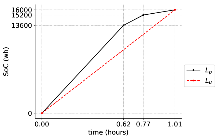
(a) Underestimated linear approximation

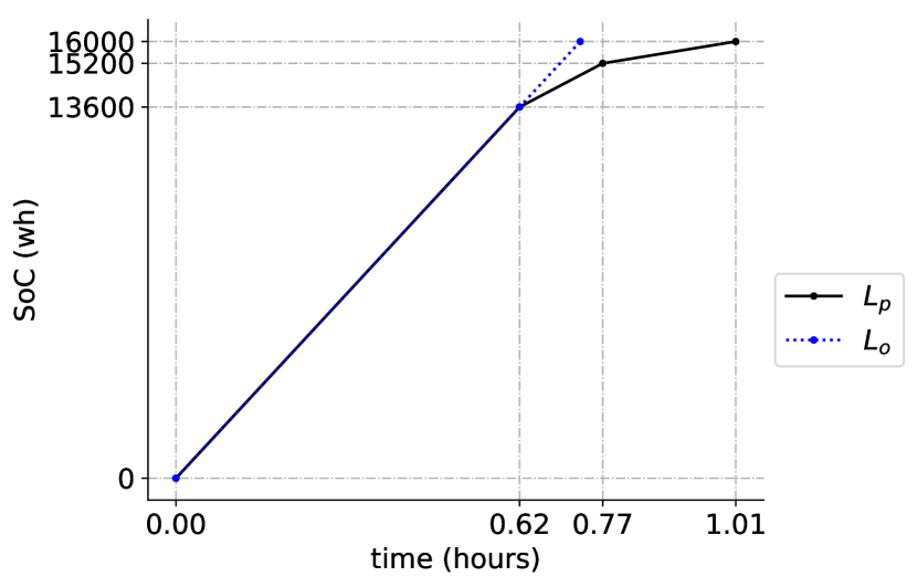
(b) Overestimated linear approximation

Figure 5: Piecewise linear function VS linear charging function

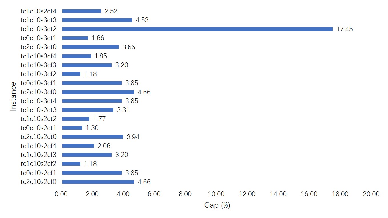
Figure 6: Comparison on cost of instances with 10 customers using piecewise linear function and underestimate linear function

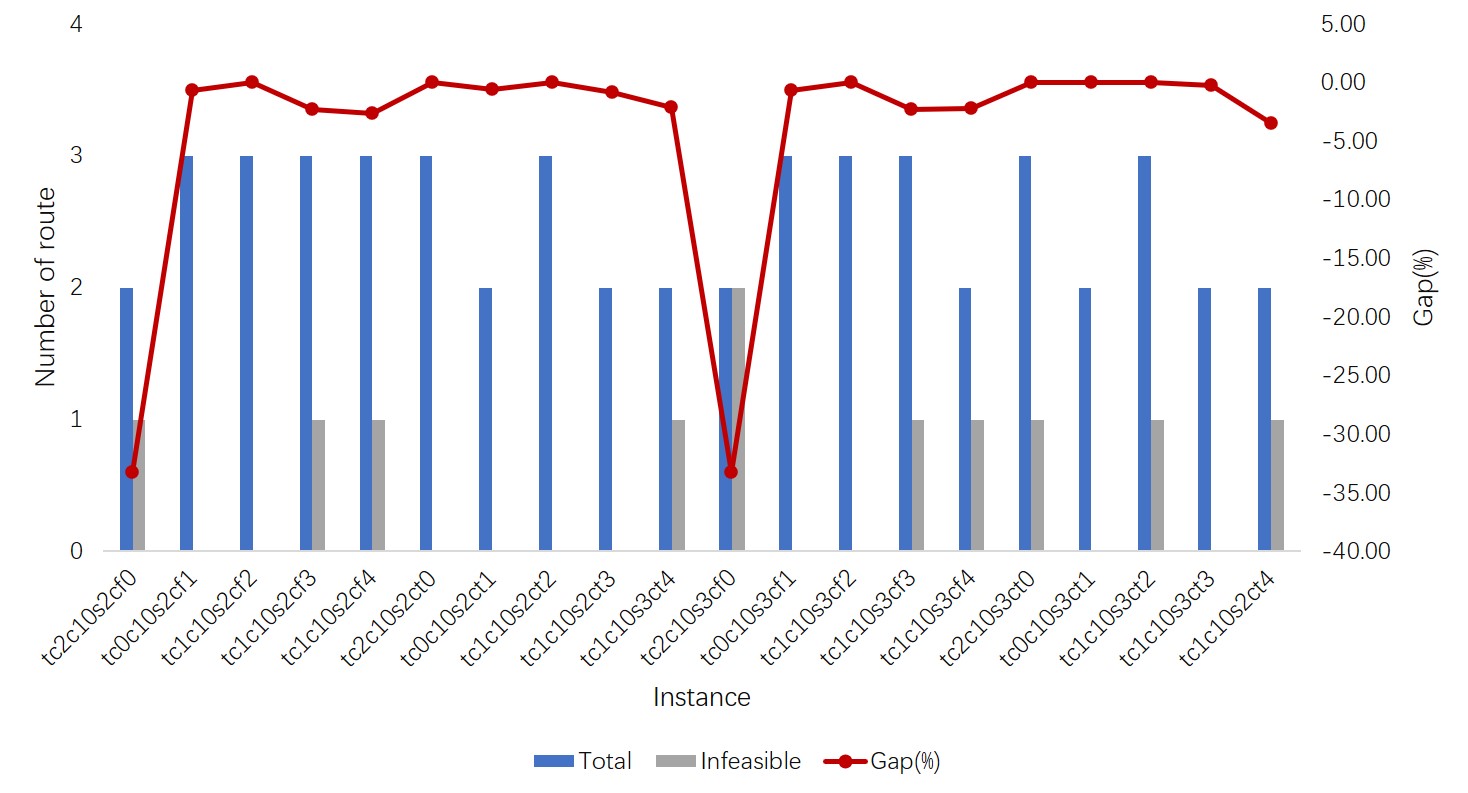
Figure 7: Comparison on results of instances with 10 customers using piecewise linear function and overestimate linear function

8 Conclusion

EVs are a potential instrument to face environmental challenges. Yet, they suffer from technical weaknesses that prevent their wider uptake and render the management and planning of transportation operations a challenging task. This paper outlines exact and heuristic algorithms to solve the E-VRP-NL introduced by Montoya et al. (2017). The nonlinear battery charging process is hard to capture in optimization models, and hence is approximated by a linear piecewise function to render models tractable and facilitate the development of efficient algorithms. However, including the piecewise linear function significantly complicates the pricing problem where both routing and charging decisions must be handled simultaneously. We formulate the E-VRP-NL as a set-partitioning model. We introduce tailored recursive functions that capture both decisions and show how we can efficiently embed them in the underlying column generation algorithm. This results in an efficient exact algorithm for the E-VRP-NL. Next to the exact algorithm, a tabu search based heuristic is also developed to solve large instances quickly.

To assess the performance of the proposed algorithms, we test them on benchmark instances provided by Montoya et al. (2017) and compare with state-of-the-art algorithms from the literature. The computational results demonstrate that our exact algorithm is capable of solving medium-scale instances to optimality, clearly outperforming existing tools. Furthermore, the proposed tabu search heuristic proves to be superior to existing heuristic algorithms from the literature. In fact, the tabu search heuristic obtain optimal solutions on small-scale instances and substantially improve the results from the literature on large-scale instances.

Because existing algorithms for the E-VRP-NL can only solve medium-size problems, there is room for improvement and multiple directions for future research are identified. First, current algorithms could be further improved by e.g., exploring the exploitation of problem specific valid inequalities and other techniques to accelerate the solution time. Second, other variants of the E-VRP-NL could be explored where e.g., the availability of CSs is probabilistic.

References

- Afroditi et al. (2014) Afroditi, Anagnostopoulou, Maria Boile, Sotirios Theofanis, Eleftherios Sdoukopoulos, Dimitrios Margaritis. 2014. Electric vehicle routing problem with industry constraints: trends and insights for future research. Transportation Research Procedia 3 452–459.
- Andelmin and Bartolini (2017) Andelmin, Juho, Enrico Bartolini. 2017. An exact algorithm for the green vehicle routing problem. Transportation Science 51(4) 1288–1303.
- Arslan and Karaşan (2016) Arslan, Okan, Oya Ekin Karaşan. 2016. A benders decomposition approach for the charging station location problem with plug-in hybrid electric vehicles. Transportation Research Part B: Methodological 93 670–695.
- Baldacci et al. (2011) Baldacci, Roberto, Aristide Mingozzi, Roberto Roberti. 2011. New route relaxation and pricing strategies for the vehicle routing problem. Operations research 59(5) 1269–1283.
- Basso et al. (2019) Basso, Rafael, Balázs Kulcsár, Bo Egardt, Peter Lindroth, Ivan Sanchez-Diaz. 2019. Energy consumption estimation integrated into the electric vehicle routing problem. Transportation Research Part D: Transport and Environment 69 141–167.
- Bektaş and Laporte (2011) Bektaş, Tolga, Gilbert Laporte. 2011. The pollution-routing problem. Transportation Research Part B: Methodological 45(8) 1232–1250.
- Boland et al. (2006) Boland, Natashia, John Dethridge, Irina Dumitrescu. 2006. Accelerated label setting algorithms for the elementary resource constrained shortest path problem. Operations Research Letters 34(1) 58–68.
- Breunig et al. (2019) Breunig, Ulrich, Roberto Baldacci, Richard F Hartl, Thibaut Vidal. 2019. The electric two-echelon vehicle routing problem. Computers & Operations Research 103 198–210.
- Bruglieri et al. (2015) Bruglieri, Maurizio, Ferdinando Pezzella, Ornella Pisacane, Stefano Suraci. 2015. A variable neighborhood search branching for the electric vehicle routing problem with time windows. Electronic Notes in Discrete Mathematics 47 221–228.
- Christofides et al. (1981) Christofides, Nicos, Aristide Mingozzi, Paolo Toth. 1981. Exact algorithms for the vehicle routing problem, based on spanning tree and shortest path relaxations. Mathematical programming 20(1) 255–282.
- Costa et al. (2019) Costa, Luciano, Claudio Contardo, Guy Desaulniers. 2019. Exact branch-price-and-cut algorithms for vehicle routing. Transportation Science 53(4) 946–985.
- Dabia et al. (2017) Dabia, Said, Emrah Demir, Tom Van Woensel. 2017. An exact approach for a variant of the pollution-routing problem. Transportation Science 51(2) 607–628.
- Desaulniers et al. (2016) Desaulniers, Guy, Fausto Errico, Stefan Irnich, Michael Schneider. 2016. Exact algorithms for electric vehicle-routing problems with time windows. Operations Research 64(6) 1388–1405.
- Edison Electric Institute (2019) Edison Electric Institute, EEI. 2019. Electric vehicle sales: Facts & figures. https://www.eei.org/issuesandpolicy/electrictransportation/Documents/FINAL_EV_Sales_Update_April2019.pdf.
- Erdoğan and Miller-Hooks (2012) Erdoğan, Sevgi, Elise Miller-Hooks. 2012. A green vehicle routing problem. Transportation Research Part E: Logistics and Transportation Review 48(1) 100–114.
- Feillet et al. (2004) Feillet, Dominique, Pierre Dejax, Michel Gendreau, Cyrille Gueguen. 2004. An exact algorithm for the elementary shortest path problem with resource constraints: Application to some vehicle routing problems. Networks: An International Journal 44(3) 216–229.
- Felipe et al. (2014) Felipe, Ángel, M Teresa Ortuño, Giovanni Righini, Gregorio Tirado. 2014. A heuristic approach for the green vehicle routing problem with multiple technologies and partial recharges. Transportation Research Part E: Logistics and Transportation Review 71 111–128.
- Figliozzi (2010) Figliozzi, Miguel. 2010. Vehicle routing problem for emissions minimization. Transportation Research Record 2197(1) 1–7.
- Froger et al. (2018) Froger, Aurélien, Jorge E Mendoza, Ola Jabali, Gilbert Laporte. 2018. The electric vehicle routing problem with nonlinear charging functions and capacitated charging stations.
- Froger et al. (2019) Froger, Aurélien, Jorge E Mendoza, Ola Jabali, Gilbert Laporte. 2019. Improved formulations and algorithmic components for the electric vehicle routing problem with nonlinear charging functions. Computers & Operations Research 104 256–294.
- Froger et al. (2017) Froger, Aurélien, Jorge E Mendoza, Gilbert Laporte, Ola Jabali. 2017. New formulations for the electric vehicle routing problem with nonlinear charging functions .
- Ge (2013) Ge, Zhihao. 2013. The carbon emission intensity in tranportation industry is six times of that in construction industry. http://www.tanpaifang.com/tanjiliang/2013/1216/27028.html.
- Glover (1989) Glover, Fred. 1989. Tabu search part i. ORSA Journal on computing 1(3) 190–206.
- Goeke and Schneider (2015) Goeke, Dominik, Michael Schneider. 2015. Routing a mixed fleet of electric and conventional vehicles. European Journal of Operational Research 245(1) 81–99.
- Hiermann et al. (2019) Hiermann, Gerhard, Richard F Hartl, Jakob Puchinger, Thibaut Vidal. 2019. Routing a mix of conventional, plug-in hybrid, and electric vehicles. European Journal of Operational Research 272(1) 235–248.
- Hiermann et al. (2016) Hiermann, Gerhard, Jakob Puchinger, Stefan Ropke, Richard F Hartl. 2016. The electric fleet size and mix vehicle routing problem with time windows and recharging stations. European Journal of Operational Research 252(3) 995–1018.
- Hof et al. (2017) Hof, Julian, Michael Schneider, Dominik Goeke. 2017. Solving the battery swap station location-routing problem with capacitated electric vehicles using an avns algorithm for vehicle-routing problems with intermediate stops. Transportation Research Part B Methodological 97 102–112.
- Jepsen et al. (2008) Jepsen, Mads, Bjørn Petersen, Simon Spoorendonk, David Pisinger. 2008. Subset-row inequalities applied to the vehicle-routing problem with time windows. Operations Research 56(2) 497–511.
- Jie et al. (2019) Jie, Wanchen, Jun Yang, Min Zhang, Yongxi Huang. 2019. The two-echelon capacitated electric vehicle routing problem with battery swapping stations: Formulation and efficient methodology. European Journal of Operational Research 272(3) 879–904.
- Keskin and Çatay (2015) Keskin, Merve, Bülent Çatay. 2015. The electric vehicle routing problem: outlook and recharging strategies .
- Keskin and Çatay (2016) Keskin, Merve, Bülent Çatay. 2016. Partial recharge strategies for the electric vehicle routing problem with time windows. Transportation Research Part C: Emerging Technologies 65 111–127.
- Keskin and Çatay (2018) Keskin, Merve, Bülent Çatay. 2018. A matheuristic method for the electric vehicle routing problem with time windows and fast chargers. Computers & Operations Research 100 172–188.
- Koç et al. (2019) Koç, Çağrı, Ola Jabali, Jorge E Mendoza, Gilbert Laporte. 2019. The electric vehicle routing problem with shared charging stations. International Transactions in Operational Research 26(4) 1211–1243.
- Lee (2020) Lee, Chungmok. 2020. An exact algorithm for the electric-vehicle routing problem with nonlinear charging time. Journal of the Operational Research Society 1–24.
- Lin et al. (2016) Lin, Jane, Wei Zhou, Ouri Wolfson. 2016. Electric vehicle routing problem. Transportation Research Procedia 12 508–521.
- Luo et al. (2016) Luo, Zhixing, Hu Qin, Wenbin Zhu, Andrew Lim. 2016. Branch and price and cut for the split-delivery vehicle routing problem with time windows and linear weight-related cost. Transportation Science 51(2) 668–687.
- Macrina et al. (2019a) Macrina, Giusy, Gilbert Laporte, Francesca Guerriero, Luigi Di Puglia Pugliese. 2019a. An energy-efficient green-vehicle routing problem with mixed vehicle fleet, partial battery recharging and time windows. European Journal of Operational Research 276(3) 971–982.
- Macrina et al. (2019b) Macrina, Giusy, Luigi Di Puglia Pugliese, Francesca Guerriero, Gilbert Laporte. 2019b. The green mixed fleet vehicle routing problem with partial battery recharging and time windows. Computers & Operations Research 101 183–199.
- Martinelli et al. (2014) Martinelli, Rafael, Diego Pecin, Marcus Poggi. 2014. Efficient elementary and restricted non-elementary route pricing. European Journal of Operational Research 239(1) 102–111.
- MEE (2017) MEE, Ministry of Ecology & Environment of the People’s Republic of China. 2017. Limits and measurement methods for emissions from light-duty vehicles (china 6). https://english.mee.gov.cn/Resources/standards/Air_Environment/emission_mobile/.
- Montoya et al. (2015) Montoya, Alejandro, Christelle Guéret, Jorge E Mendoza, Juan Villegas. 2015. The electric vehicle routing problem with partial charging and nonlinear charging function .
- Montoya et al. (2017) Montoya, Alejandro, Christelle Guéret, Jorge E Mendoza, Juan G Villegas. 2017. The electric vehicle routing problem with nonlinear charging function. Transportation Research Part B: Methodological 103 87–110.
- Pelletier et al. (2016) Pelletier, Samuel, Ola Jabali, Gilbert Laporte. 2016. 50th anniversary invited article-goods distribution with electric vehicles: Review and research perspectives. Transportation Science 50(1) 3–22.
- Pelletier et al. (2018) Pelletier, Samuel, Ola Jabali, Gilbert Laporte. 2018. Charge scheduling for electric freight vehicles. Transportation Research Part B: Methodological 115 246–269.
- Pelletier et al. (2017) Pelletier, Samuel, Ola Jabali, Gilbert Laporte, Marco Veneroni. 2017. Battery degradation and behaviour for electric vehicles: Review and numerical analyses of several models. Transportation Research Part B: Methodological 103 158–187.
- Preis et al. (2014) Preis, Henning, Stefan Frank, Karl Nachtigall. 2014. Energy-optimized routing of electric vehicles in urban delivery systems. Operations Research Proceedings 2012. Springer, 583–588.
- Righini and Salani (2006) Righini, Giovanni, Matteo Salani. 2006. Symmetry helps: Bounded bi-directional dynamic programming for the elementary shortest path problem with resource constraints. Discrete Optimization 3(3) 255–273.
- Sassi et al. (2014) Sassi, Ons, Wahiba Ramdane Cherif, Ammar Oulamara. 2014. Vehicle routing problem with mixed fleet of conventional and heterogenous electric vehicles and time dependent charging costs .
- Sassi et al. (2015) Sassi, Ons, Wahiba Ramdane Cherif-Khettaf, Ammar Oulamara. 2015. Iterated tabu search for the mix fleet vehicle routing problem with heterogenous electric vehicles. Modelling, Computation and Optimization in Information Systems and Management Sciences. Springer, 57–68.
- Schiffer and Walther (2017) Schiffer, Maximilian, Grit Walther. 2017. The electric location routing problem with time windows and partial recharging. European Journal of Operational Research 260(3) 995–1013.
- Schneider et al. (2014) Schneider, Michael, Andreas Stenger, Dominik Goeke. 2014. The electric vehicle-routing problem with time windows and recharging stations. Transportation Science 48(4) 500–520.
- Sweda et al. (2017) Sweda, Timothy M, Irina S Dolinskaya, Diego Klabjan. 2017. Adaptive routing and recharging policies for electric vehicles. Transportation Science 51(4) 1326–1348.
- Tilk et al. (2017) Tilk, Christian, Ann-Kathrin Rothenbächer, Timo Gschwind, Stefan Irnich. 2017. Asymmetry matters: Dynamic half-way points in bidirectional labeling for solving shortest path problems with resource constraints faster. European Journal of Operational Research 261(2) 530–539.
- United States Environmental Protection Agency (2017) United States Environmental Protection Agency, EPA. 2017. Sources of greenhouse gas emissions. https://www.epa.gov/ghgemissions/sources-greenhouse-gas-emissions.
- Yang and Sun (2015) Yang, Jun, Hao Sun. 2015. Battery swap station location-routing problem with capacitated electric vehicles. Computers & Operations Research 55 217–232.
- Zhang et al. (2018) Zhang, Shuai, Yuvraj Gajpal, S S Appadoo, M M S Abdulkader. 2018. Electric vehicle routing problem with recharging stations for minimizing energy consumption. International Journal of Production Economics 203 404–413.