Memorize, Factorize, or be Naïve: Learning Optimal Feature Interaction Methods for CTR Prediction

Abstract

Click-through rate prediction is one of the core tasks in commercial recommender systems. It aims to predict the probability of a user clicking a particular item given user and item features. As feature interactions bring in non-linearity, they are widely adopted to improve the performance of CTR prediction models. Therefore, effectively modelling feature interactions has attracted much attention in both the research and industry field. The current approaches can generally be categorized into three classes: (i) naïve methods, which do not model feature interactions and only use original features; (ii) memorized methods, which memorize feature interactions by explicitly viewing them as new features and assigning trainable embeddings; (iii) factorized methods, which learn latent vectors for original features and implicitly model feature interactions through factorization functions. Studies have shown that modelling feature interactions by one of these methods alone are suboptimal due to the unique characteristics of different feature interactions. To address this issue, we first propose a general framework called OptInter which finds the most suitable modelling method for each feature interaction. Different state-of-the-art deep CTR models can be viewed as instances of OptInter. To realize the functionality of OptInter, we also introduce a learning algorithm that automatically searches for the optimal modelling method. We conduct extensive experiments on four large datasets, including three public and one private. Experimental results demonstrate the effectiveness of OptInter. Because our OptInter finds the optimal modelling method for each feature interaction, our experiments show that OptInter improves the best performed state-of-the-art baseline deep CTR models by up to 2.21%. Compared to the memorized method, which also outperforms baselines, we reduce up to 91% parameters. In addition, we conduct several ablation studies to investigate the influence of different components of OptInter. Finally, we provide interpretable discussions on the results of OptInter.

I Introduction

The Click-through rate (CTR) prediction task is crucial for recommender systems, which aims to predict the probability of a certain user clicking on a recommended item (e.g. movie, advertisement)[1, 2, 3, 4]. Many recommendations can therefore be performed based on the result of CTR prediction. For instance, to maximize the number of clicks, the items returned to a user can be ranked by predicted CTR (pCTR).

Due to the powerful featur e representation learning ability, the mainstream of CTR prediction research is dominated by deep learning models. As an important research direction to improve deep CTR models, many methods of modelling effective feature interactions are proposed, such as [5, 2, 1, 3, 4].

The simplest way of modelling feature interactions is feeding original features in Multi-layer Perceptron (MLP). Shown as an example in Figure  1(a), FNN [5] directly feeds original features into MLP and relies on the capability of MLP to model feature interactions. The universal approximation rule has proved that MLP can mimic arbitrary functions given enough data and computation power [6]. However, it is challenging for MLP to model low-rank feature interactions solely based on original features [7]. Such a way of modelling feature interactions by MLP directly is referred to as naïve methods in our paper.

Another alternative to model feature interactions is memorizing them explicitly as new features, named as memorized methods. These methods [8, 1] which memorize all second-order feature interactions as new features and feed them in shallow models (as shown in Figure 1(b), feature interactions are treated as individual features and fed into the wide component), achieve superior performance than naïve methods. The reason is that some feature interactions are served as strong signals such that memorizing them as new features makes correlated patterns much easier to capture. However, memorized methods are prone to overfitting as the new features (generated by feature interactions) are more sparse and have lower frequency than original features in the training set.

The final method is to model feature interactions via a factorization function, named as factorized method. It is originated from Factorization Machine (FM) [9] and its variants [10, 11, 12]. Factorized methods implicitly model all second-order feature interactions by learning latent vectors of original features and aggregating them using a specific function (e.g., inner-product) [9, 10] or learnable factorization function [11, 12], as shown in Figure 1(c). Factorized methods alleviate the feature sparsity issue and are widely adopted by the mainstream deep CTR models [2, 3, 4]. However, the latent vectors are used in both representation learning and feature interaction modelling, which tends to conflict with each other.

The above three methods (namely, naïve, memorized, factorized methods) model all possible feature interactions in an identical way. However, as stated in [15], modelling feature interactions in the same way may lead to a suboptimal solution because the characteristics (e.g., complexity) of each feature interaction may not be identical. Hence, AutoML methods [16, 17] are introduced to find an appropriate modelling method for each feature interaction [15, 18]. For instance, AutoFIS [15] aims to select which feature interactions should be factorized and which ones should be ignored. In other words, AutoFIS makes a choice between factorized and naïve adaptively for each individual feature interaction, while the option of memorized is neglected.

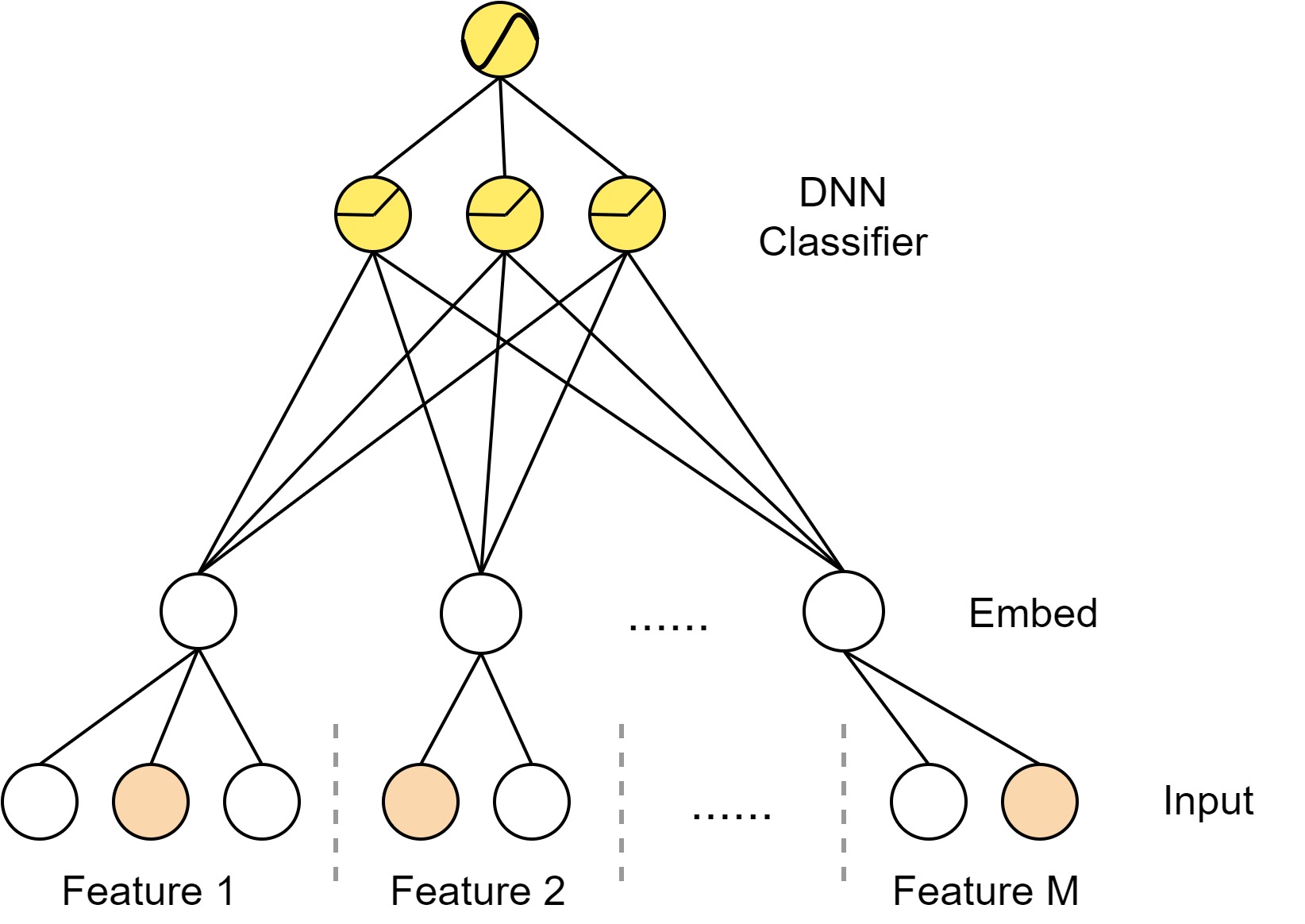
(a) FNN

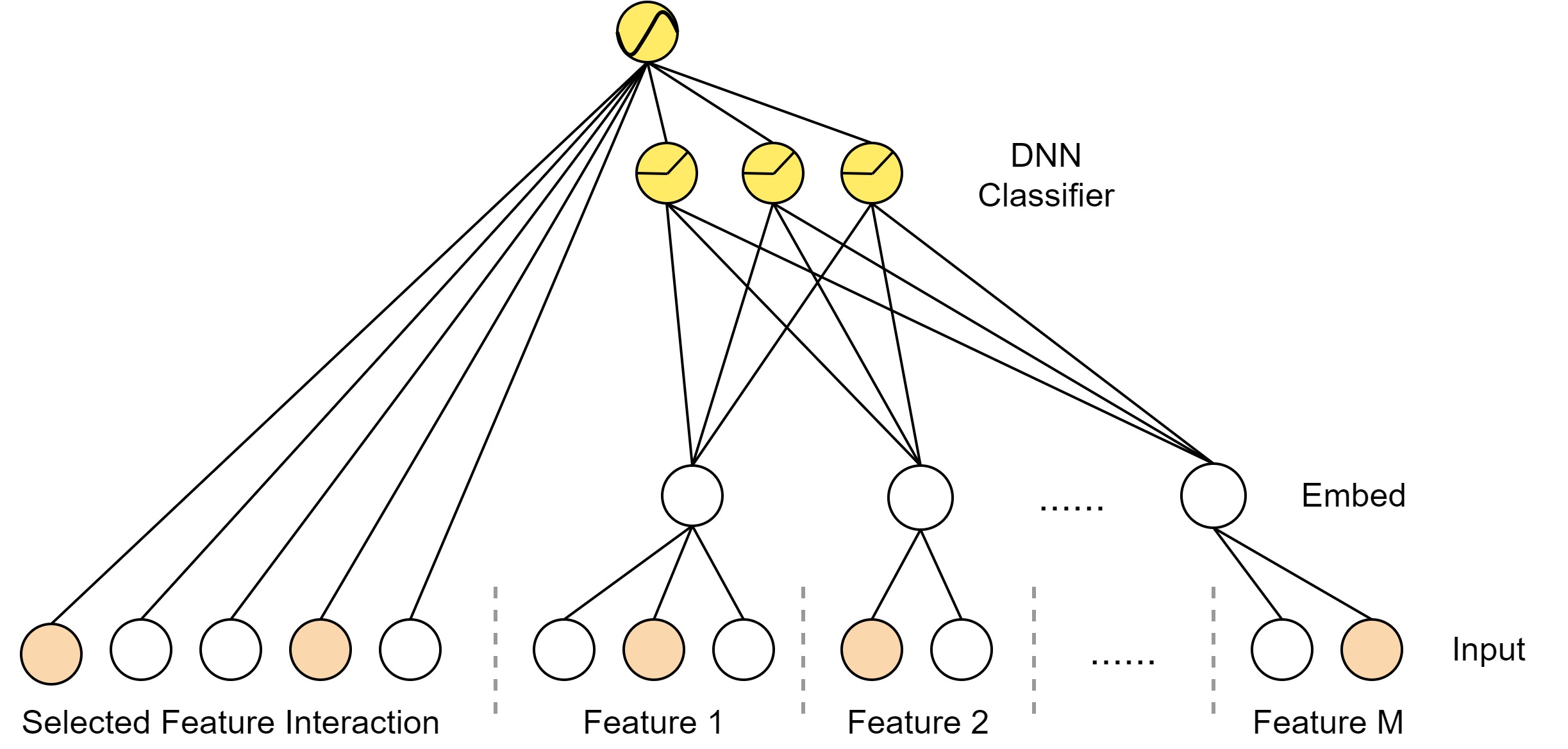
(b) Wide&Deep

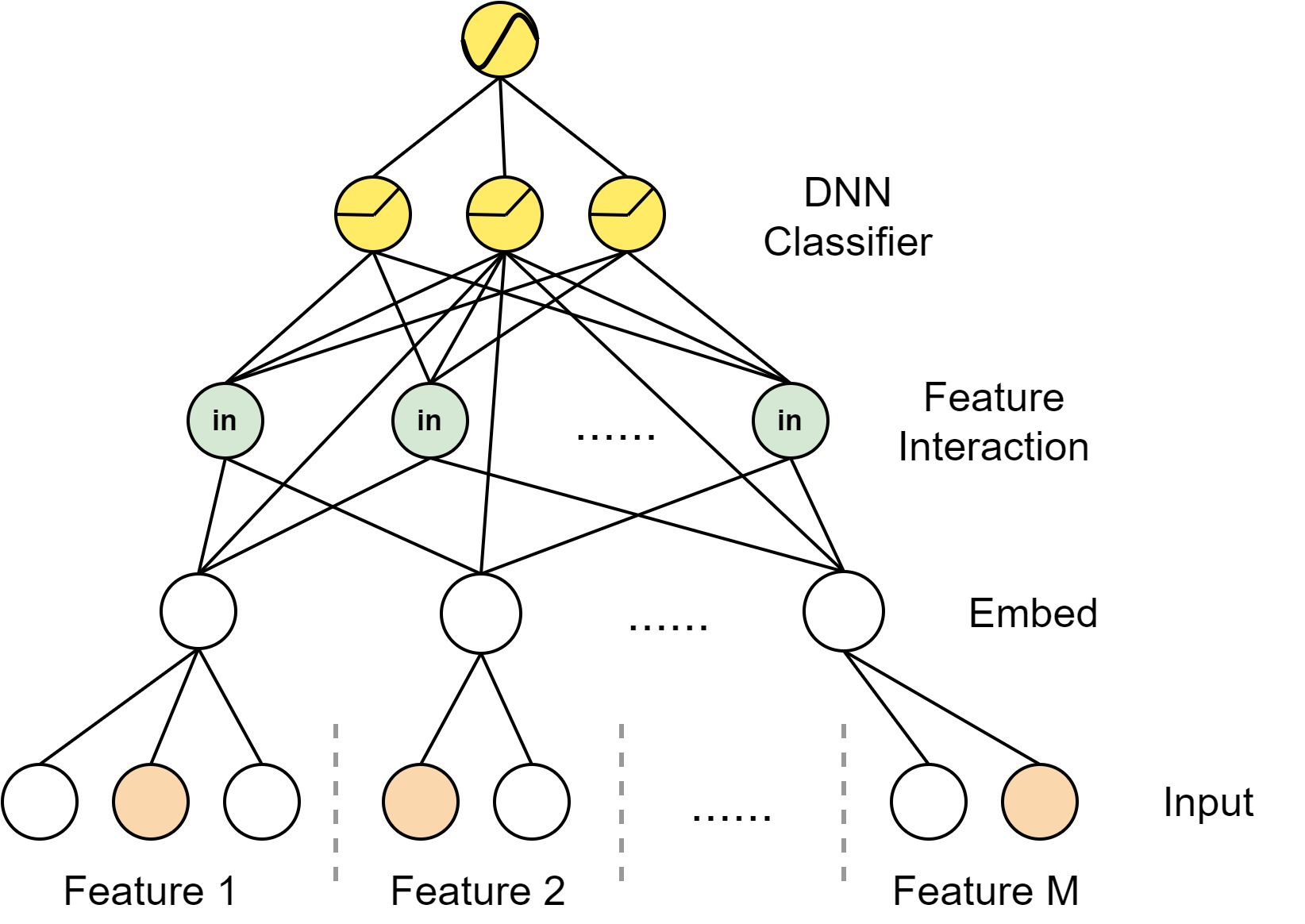
(c) IPNN

Figure 1: Examples of modeling feature interactions: Naïve, Memorized and Factorized

With the limitations of prior research observed, a data-driven strategy to automatically find an optimal method from naïve, memorized, factorized methods for each feature interaction is required. This motivates us to propose a general framework called OptInter. For each feature interaction, OptInter selects the optimal modelling method from naïve, memorized, factorized methods adaptively and automatically. Inspired by DARTS [16] and previous works [15, 18], to efficiently search the optimal method for each feature interaction, we devise a two-stage learning algorithm. In the search stage, we aim to select the optimal method for each feature interaction from the search space naïve, memorized, factorized, where the selection is treated as a neural architecture search problem. However, such a selection is discrete and makes the overall framework not differentiable. Therefore, instead of searching over three candidate modelling methods, we relax the choices to be continuous by approximating with Gumbel-softmax tricks[19] via a set of architecture parameters (one for each modelling method with respect to a feature interaction). Then, the architecture parameters can be learned by gradient descent, which is jointly optimized with neural network weights. In the re-train stage, we select the modelling method with the largest probability for each feature interaction and re-train the model from scratch. The neural network weights obtained from the search stage are discarded to avoid the influence of suboptimal modelling methods.

Extensive experiments are conducted on four large-scale datasets, including three public datasets and one private dataset. Experimental results demonstrate OptInter consistently performs well on all datasets. Specifically, memorized method improves the best performed deep CTR model by 0.1%-2.2% in terms of the AUC score with the help of 18 times more parameters. Moreover, compared to the memorized method, OptInter achieves further improvement of AUC by 0.01%-0.25% while reduces about 18%-91% parameters. The results demonstrate the effectiveness of introducing memorized method in our search space and the efficiency of OptInter by selecting suitable modelling methods for individual feature interactions. Our ablation studies also show that our proposed search algorithm yields a more effective architecture than other search algorithms. Last but not least, we analyze the search architecture of OptInter from the perspective of information theory and provide interpretability. To sum up, the main contributions of this paper are:

1. We propose a novel deep CTR prediction framework OptInter including naïve, memorized, factorized feature interaction methods. To our best knowledge, OptInter is the first work to introduce memorized method in deep CTR models. Moreover, some mainstream deep CTR methods can be viewed as instances of OptInter.

2. As a part of OptInter, we propose a two-stage learning algorithm to select the optimal method for each feature interaction automatically. In the search stage, OptInter can learn the relative importance of each feature interaction method via architecture parameters. In the re-train stage, with the resulting optimal methods, we re-train the model from scratch to guarantee the neural network is not influenced by suboptimal methods.

3. Comprehensive experiments are conducted on three public datasets and one private dataset and show that OptInter outperforms the state-of-the-art deep CTR prediction models. The results demonstrate that OptInter is both effective and efficient.

II Methodology

In this section, we first formulate the problem of CTR prediction task and feature interaction modelling methods in Section II-A. Then we describe the proposed framework OptInter in Section II-B. Finally, we elaborate details of the learning algorithm for OptInter in Section II-C. To make our framework easier to understand, we list all the notations used in Table I.

II-A Problem Formulation

II-A1 CTR Prediction

A dataset for training CTR models consists of instances $(\mathbf{X}^{o},y)$, where $y\in\{0,1\}$ is the ground truth label and $\mathbf{X}^{o}$ is a multi-field data instance including $M$ original features

$$\mathbf{X}^{o}=[\mathbf{x}^{o}_{1},\mathbf{x}^{o}_{2},...,\mathbf{x}^{o}_{M}],$$ (1)

where $\mathbf{x}^{o}_{i}$ is the one-hot encoded vector for the feature value in the $i$-th original feature. The problem of CTR prediction is to predict the probability of a user clicking a certain item according to original features $\mathbf{X}^{o}$. Formally, a machine learning model to estimate the probability is defined as follows,

$$\mathbf{P}(y=1|\mathbf{X}^{o})=f(\mathbf{X}^{o};\Theta),$$ (2)

where $f$ is the model, ${\Theta}$ indicates all the model parameters, and $\mathbf{P}$ is the conditional probability.

TABLE I: Selected notations in this paper

Notations	Descriptions
$y$	ground truth label
$\hat{y}$	predicted result
$\mathbf{X}^{o}$	original features
$\mathbf{X}^{m}$	cross-product transformed features
$\mathbf{x}^{o}_{i}$	original feature $i$
$\mathbf{e}^{o}_{i}$	embedding for original feature $i$
$\mathbf{e}^{f}_{(i,j)}$	factorized embedding for $(\mathbf{x}^{o}_{i},\mathbf{x}^{o}_{j})$
$\mathbf{x}^{m}_{(i,j)}$	cross-product transformed features for $(\mathbf{x}^{o}_{i},\mathbf{x}^{o}_{j})$
$\mathbf{e}^{m}_{(i,j)}$	memorized embedding for $(\mathbf{x}^{o}_{i},\mathbf{x}^{o}_{j})$
$\mathbf{e}^{n}$	null embedding
$\mathbf{e}^{b}_{(i,j)}$	optimal embedding for $(\mathbf{x}^{o}_{i},\mathbf{x}^{o}_{j})$
$M$	number of original feature
$\mathcal{K}$	searchable modelling space
$\mathcal{D}$	dataset
$\times$	cross product
$\Theta$	model parameter
$\alpha$	architecture parameter

II-A2 Feature Interaction

Feature interactions capture the correlation between different features and induce non-linearity to the model. As shown in existing works, it is crucial to model feature interactions to boost the model performance [3, 4, 2, 1, 5].

In this section, we formally define the feature interaction and introduce three modelling methods.

Definition 1.

A $h$-th order ($1\leq h\leq M$) feature interaction $\mathcal{H}$ is defined as a multivariate group $(\mathbf{x}^{o}_{c_{1}},\mathbf{x}^{o}_{c_{2}},...,\mathbf{x}^{o}_{c_{h}})$, where each feature $\mathbf{x}^{o}_{c_{i}}$ is selected from original feature $\mathbf{X}^{o}$.

Generally, there are three methods to define feature interaction:

(i) Factorized method: Given the latent vectors for original features $\mathbf{E}^{o}$, $\mathcal{H}$ can be modelled as[20]

$$\begin{split}\mathbf{e}^{f}_{\mathcal{H}}&=o^{(h-1)}(...(o^{(1)}(\mathbf{e}^{o}_{c_{1}},\mathbf{e}^{o}_{c_{2}})),...,\mathbf{e}^{o}_{c_{h}}),\\ \mathbf{e}^{o}_{c_{i}}&=\mathbf{E}^{o}\mathbf{x}^{o}_{c_{i}}.\end{split}$$ (3)

Namely, the factorized embedding $\mathbf{e}^{f}_{\mathcal{H}}$ is generated by the utilizing $h-1$ operators $o^{(1)}(\cdot)$, $o^{(2)}(\cdot)$, .., $o^{(h-1)}(\cdot)$ in order to aggregate $h$ latent vectors $\mathbf{e}^{o}_{c_{1}}$, $\mathbf{e}^{o}_{c_{2}}$, …, $\mathbf{e}^{o}_{c_{h}}$. Here the operators could be FM, inner product or etc.

(ii) Memorized method: Memorized embedding $\mathbf{e}^{m}_{\mathcal{H}}$ can be defined as[21]

$$\begin{split}\mathbf{e}^{m}_{\mathcal{H}}&=\mathbf{E}^{m}\mathbf{x}^{m}_{\mathcal{H}},\\ \mathbf{x}^{m}_{\mathcal{H}}&=\text{onehot}(\mathbf{\bar{x}}^{o}_{c_{1}}\times\mathbf{\bar{x}}^{o}_{c_{2}}\times...\times\mathbf{\bar{x}}^{o}_{c_{h}}),\end{split}$$ (4)

where $\mathbf{\bar{x}}^{o}_{c_{i}}$ is zero-padded original feature $\mathbf{x}^{o}_{c_{i}}$ (zero-padding is introduced to align the dimension), $\times$ is the cross-product operation, $\mathbf{x}^{m}_{\mathcal{H}}$ is the cross-product transformed feature for $\mathcal{H}$, $\mathbf{E}^{m}$ is the embedding table for cross-product transformed features.

(iii) Naïve method: the naïve embedding $\mathbf{e}^{n}_{\mathcal{H}}=\mathbf{e}^{n}$ can be defined as a zero vector with arbitrary length. Note that for different $\mathcal{H}$, the naïve embedding $\mathbf{e}^{n}$ remains the same.

II-B OptInter Framework

In this section, we elaborate the OptInter framework in detail, which is presented in Figure 2. The OptInter framework consists of four components: (i) the input layer (Section II-B1), (ii) the embedding layer (Section II-B2), (iii) the feature interaction layer (Section II-B3) and (iv) the classifier (Section II-B4). The feature interaction layer plays a central part in OptInter and greatly influences the performance, where the combination block searches the optimal method for each individual feature interaction.

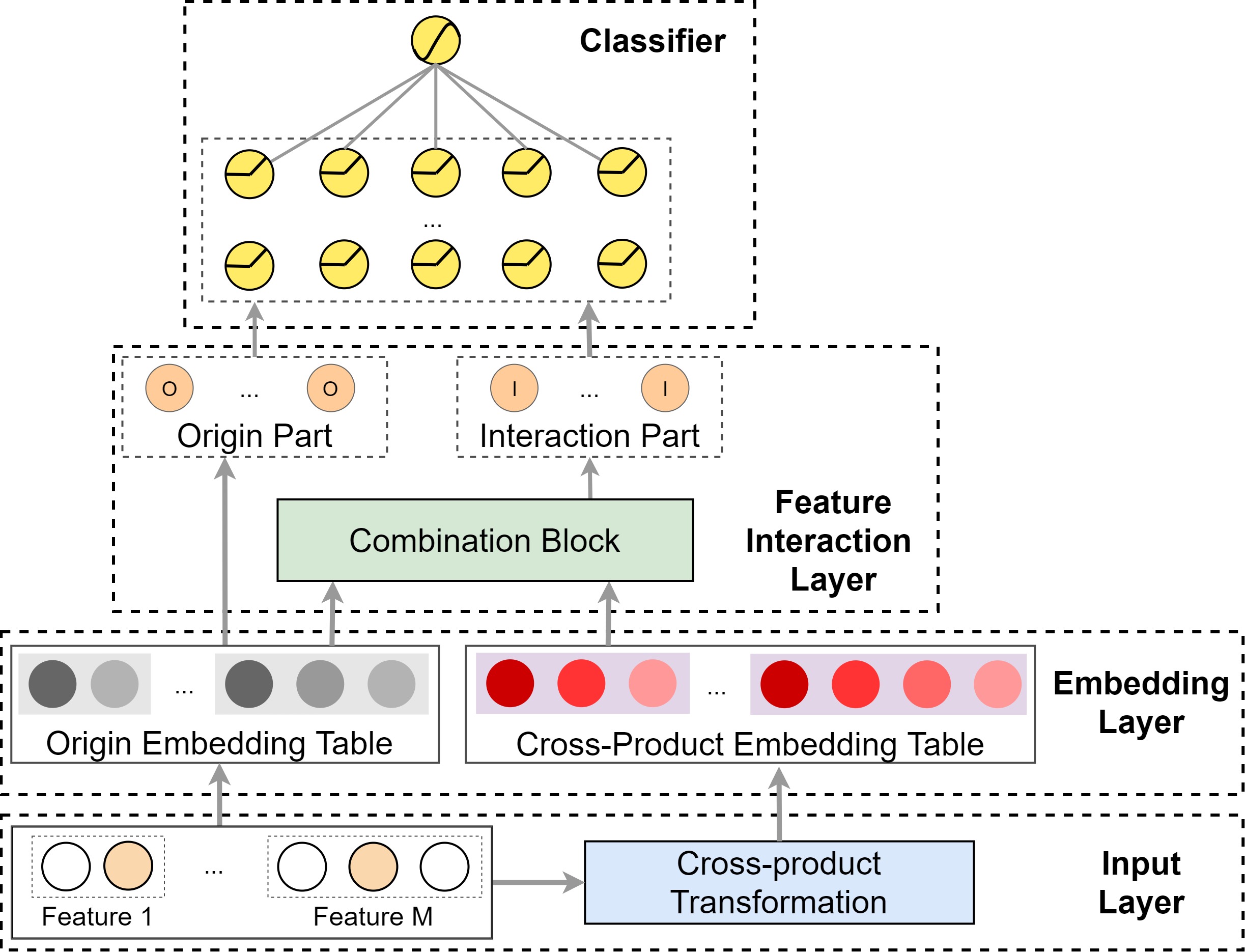
Figure 2: The OptInter CTR Framework

In OptInter, Equation 2 is specified to estimate the probability for input $\mathbf{X^{o}}$ as follows,

$$\begin{split}\hat{y}=f(\mathbf{X}^{o}|\Theta,\alpha),\end{split}$$ (5)

where $f(\cdot)$ indicates the OptInter framework, $\Theta$ indicates all the neural network parameters and $\alpha$ indicates the architecture parameters. Such architecture parameters in combination block decide which modelling method to choose for each feature interaction.

II-B1 Input Layer

In OptInter, the input layer contains a cross-product transformation block, which takes original features $\mathbf{X}^{o}$ as input and generates one-hot encoded representation $\mathbf{X}^{m}$ according to Equation 4. Note that for $M$ original features, there are $C^{h}_{M}$ $h$-th order feature interactions. In OptInter, we only consider the second-order feature interactions (namely, $h=2$) for two reasons: (i) second-order feature interactions have been demonstrated to be the most important for prediction [18] and (ii) modelling higher-order feature interactions exponentially increases the size of the embedding table and makes the current hardware difficult to train such large models. Note that although we only consider second-order feature interactions in this paper, our methods could easily be extended to higher-order. The embeddings of all the second-order feature interactions are concatenated to form

$$\mathbf{X}^{m}=[\mathbf{x}^{m}_{(1,2)},\mathbf{x}^{m}_{(1,3)},...,\mathbf{x}^{m}_{(M-1,M)}].$$ (6)

The final input includes both original feature $\mathbf{X}^{o}$ and cross-product transformed features $\mathbf{X}^{m}$ for feature interactions.

II-B2 Embedding Layer

The embedding layer is to transform the one-hot encoded features into continuous embeddings. After going through input layer, the features contains two parts: (i) original features $\mathbf{X}^{o}$ and (ii) cross-product transformed features $\mathbf{X}^{m}$. Both $\mathbf{X}^{o}$ and $\mathbf{X}^{m}$ are one-hot encoded and multi-field. All the features are in categorical form, where features in the numerical form are usually transformed into categorical form by bucketing [2, 3]. For univalent features (e.g., “Gender=Male”), we embed the one-hot encoding of each feature separately to a continuous vector using a linear embedding, i.e., the embedding $\mathbf{e}^{o}_{i}$ of feature $i$ is $\mathbf{e}^{o}_{i}=\mathbf{E}^{o}\mathbf{x}^{o}_{i}$, where $\mathbf{E}^{o}$ is the embedding table for original features. For multivalent features (e.g., “Interest=Football, Basketball”), we keep the same procedure as [3, 4, 2] where all the embeddings of individual feature values are aggregated by mean pooling. The embeddings of the original features are concatenated to form

$$\mathbf{e}^{o}=[\mathbf{e}^{o}_{1},\mathbf{e}^{o}_{2},...,\mathbf{e}^{o}_{M}].$$ (7)

The cross-product transformed features $\mathbf{X}^{m}$ for all feature interactions are also embedded to a continuous vector in the same way. For the cross-product transformed feature between original feature $\mathbf{x}^{o}_{i}$ and $\mathbf{x}^{o}_{j}$, its embedding $\mathbf{e}^{m}_{(i,j)}=\mathbf{E}^{m}\mathbf{x}^{m}_{(i,j)}$, where $\mathbf{E}^{m}$ is the embedding table for cross-product transformed features. All $\mathbf{e}^{m}_{(i,j)}$s are concatenated to form

$$\mathbf{e}^{m}=[\mathbf{e}^{m}_{(1,2)},\mathbf{e}^{m}_{(1,3)},...,\mathbf{e}^{m}_{(M-1,M)}].$$ (8)

II-B3 Feature Interaction Layer

The feature interaction layer is the nucleus of OptInter. As observed in Figure 2, we introduce a combination block to search for the optimal modelling method for each feature interaction. The combination block takes both the original feature embedding $\mathbf{e}^{o}$ and the cross-product transformed feature embedding $\mathbf{e}^{m}$ as inputs and generates embeddings $\mathbf{e}^{b}$ for all the feature interactions with the methods searched by OptInter. For each feature interaction, we search its optimal modelling method from (i) memorized method with the memorized cross-product embedding $\mathbf{e}^{m}$; (ii) factorized method with the original feature embedding $\mathbf{e}^{o}$ and factorization function; and (iii) naïve method which indicates this feature interaction is useless and does not need to modelling. We will elaborate the learning algorithm used to search the optimal method for each feature interaction in Section II-C.

II-B4 Classifier

In the feature interaction layer, $\mathbf{e}^{o}$ and $\mathbf{e}^{b}$ are concatenated into a single vector $\mathbf{e}=[\mathbf{e}^{o},\mathbf{e}^{b}]$. Similar to previous works[3, 2, 4], such vector $\mathbf{e}$ is fed into MLP, in which layer normalization and ReLU are applied. One such layer in MLP is defined as

$$\begin{split}&\mathbf{a^{(l+1)}}=\text{LN}(\text{relu}(\mathbf{W^{(l)}}\mathbf{a^{(l)}}+\mathbf{b^{(l)}})),\\ &\mathbf{a^{0}}=\mathbf{e},\end{split}$$ (9)

where $\mathbf{a^{(l)}}$, $\mathbf{W^{(l)}}$ and $\mathbf{b^{(l)}}$ are the input, model weight, and bias of the $l$-th layer. Activation ReLU is defined as

$$\text{relu}(z)=\max(0,z),$$ (10)

and layer normalization is defined as [22]

$$\textbf{LN}(z)=\frac{z-\mathcal{E}[z]}{\sqrt{\text{Var}[x]+\epsilon}}*\gamma+\beta.$$ (11)

Note that $\text{MLP}(\mathbf{a}^{(0)})=\mathbf{a}^{(h)}$, where $h$ is the depth of MLP. Finally, the output of MLP, $\mathbf{a}^{(h)}$, is fed into a sigmoid unit, in order to re-scale the prediction value to a probability. Formally, the final predicted result is

$$\hat{y}=\text{sigmoid}(\mathbf{a}^{(h)})=\frac{1}{1+e^{-\mathbf{a}^{(h)}}}\in(0,1),$$ (12)

which indicates the probability of a specific user clicking on the item. To train our CTR prediction model, we use the cross-entropy loss (i.e., log-loss) function

$$\begin{split}\mathcal{L}(\mathcal{D}|\Theta,\alpha)&=-\frac{1}{|\mathcal{D}|}\sum_{(x,y)\in\mathcal{D}}\text{CE}(y,\hat{y}),\\ \text{CE}(y,\hat{y})&=y\log(\hat{y})+(1-y)\log(1-\hat{y}),\end{split}$$ (13)

where $\mathcal{D}$ indicates the training dataset, $\Theta$ includes all the neural network weights $\{\mathbf{W^{(l)}},\mathbf{b^{(l)}}|1\leq l\leq h\}$ and embedding tables $\{\mathbf{E}^{o},\mathbf{E}^{m}\}$, $\alpha$ is the set of architecture parameters used to search the optimal feature interaction. $\alpha$ will be discussed in Section II-C.

II-C Learning Algorithm for OptInter

To find the optimal feature interaction method, we need to define a search space and devise an efficient search algorithm. In this section, we first define our search space consisting of memorized, factorized, and naïve methods for each feature interaction. Then we introduce our search algorithm to find the optimal methods efficiently. At last, we present the re-train stage for final training.

II-C1 Search Space

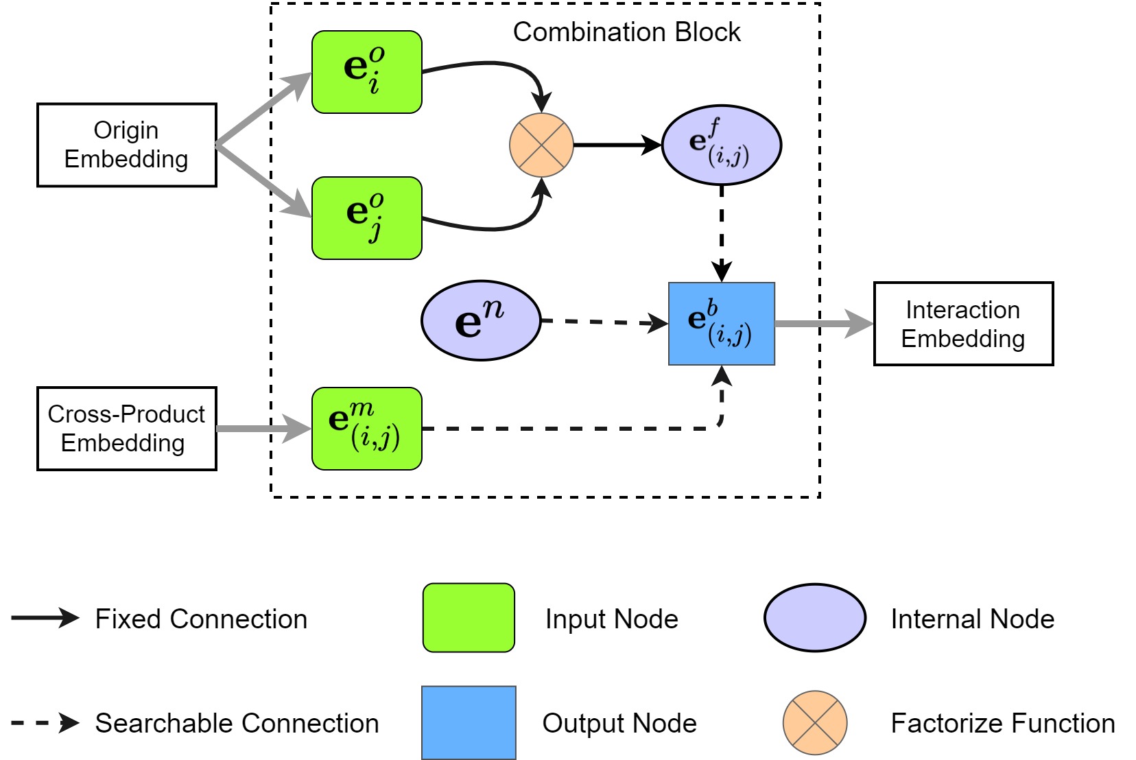
Figure 3: Detailed illustration figure about combination block

As stated in Section II-D, we categorize feature interaction methods into three classes: (i) memorized methods treat each feature interaction as a new feature and explicitly assign trainable weights or embedding. (ii) factorized methods model a feature interaction via factorization methods on latent vectors of original features. (iii) naïve methods feed the original features into MLP to model their interactions. Our search space consists of these three methods to model feature interaction. Note that there exist a wide variety of factorization functions, such as Hadamard Product $\otimes$, Pointwise-Addition $\oplus$ and Generalized-Product $\boxtimes$. In this paper, as we focus on searching the optimal modelling method (namely, memorized, factorized and naïve) for each feature interaction, we take Hadamard Product $\otimes$ as the representative for factorized methods, instead of considering all possible product operations. Our framework can be extended easily to taking multiple operations into account as factorized methods. Hadamard Product is element-wise multiplication over each element in the vectors. Formally, the Hadamard Product for feature $\mathbf{e}_{i}$ and $\mathbf{e}_{j}$ is

$$\mathbf{e}^{f}_{(i,j)}=\mathbf{e}^{o}_{i}\otimes\mathbf{e}^{o}_{j}=[e^{1}_{i}\times e^{1}_{j},e^{2}_{i}\times e^{2}_{j},...,e^{s}_{i}\times e^{s}_{j}],$$ (14)

where $e^{t}_{i}$ is the $t$-th element of the embedding for feature $i$, $s$ is the length of embedding. For each feature interation, we make the choice from 3 options. There are $C_{M}^{2}=M(M-1)/2$ second-order feature interactions in total. Therefore the total search space of OptInter is $\mathcal{O}(3^{M(M-1)/2})$, which is an incredibly huge space to search over.

The combination block is visualized in Figure 3. The final output $\mathbf{e}^{b}_{(i,j)}$ is chosen from: memorized cross-product embedding $\mathbf{e}^{m}_{(i,j)}$, factorized embedding $\mathbf{e}^{f}_{(i,j)}$ or naïve embedding $\mathbf{e}^{n}$ (which is actually empty embedding)

$$\mathbf{e}^{b}_{(i,j)}\in\{\mathbf{e}^{m}_{(i,j)},\mathbf{e}^{f}_{(i,j)},\mathbf{e}^{n}\}.$$ (15)

II-C2 Search Algorithm

Algorithm 1 The Optimization of Search Stage

1:Training dataset $\mathcal{D}$ consists of original features $(x_{1},..,x_{M})$ and ground-truth labels $y$

2:the searched optimal architecture parameter $\alpha^{*}$

3:while not converge do

4:     Sample a mini-batch of training data $\mathcal{D}_{\text{train}}$

5:     Generate the predicted labels $\hat{y}$ via OptInter with

6:  model parameter $\Theta$ and architecture parameter $\alpha$

7:  given Equation 12

8:     Calculate the cross-entropy loss $\mathcal{L}(\mathcal{D}_{\text{train}}|\Theta,\alpha)$ over

9:  the mini-batch given Equation 13

10:     Update model parameter $\Theta$ by descending gradient

11:  $\bigtriangledown_{\Theta}\mathcal{L}(\mathcal{D}_{\text{train}}|\Theta,\alpha)$

12:     Update architecture parameter $\alpha$ by descending

13:  gradient $\bigtriangledown_{\alpha}\mathcal{L}(\mathcal{D}_{\text{train}}|\Theta,\alpha)$

14:end while

In this section, we propose a search algorithm for exploring the huge search space efficiently. Instead of searching over a discrete (categorical) set of selections on the candidate methods, which will make the whole framework not end-to-end differentiable, we approximate the discrete sampling via introducing the Gumbel-softmax operation[19] in this work. The Gumbel-softmax operation provides a differentiable sampling, which makes the architecture parameters learnable by Adam optimizer.

To be specific, suppose architecture parameters $\{\alpha_{(i,j)}^{k}|k\in\mathcal{K}\}$ are the class probability over different feature interaction methods, $\mathcal{K}$ indicates the searchable space over feature interaction methods (namely, memorized, factorized, naïve). Then a discrete selection $z$ can be drawn via the gumbel-softmax trick[23] as

$$\begin{split}&z=\text{onehot}\left(\operatorname*{arg\,max}_{k\in\mathcal{K}}[\log\alpha^{k}_{(i,j)}+g_{(i,j)}]\right),\\ &g_{(i,j)}=-\log(-\log(u_{(i,j)})),\\ &u_{(i,j)}\sim\text{Uniform}(0,1).\end{split}$$ (16)

The gumbel noise $g_{(i,j)}$ is i.i.d. sampled, which aims to perturb the log term $\log\alpha_{(i,j)}^{k}$ and makes the argmax operation equivalent to drawing a sample by $\{\alpha_{(i,j)}^{k}|k\in\mathcal{K}\}$ weights. However, the argmax operation makes this trick non-differentiable. To deal with this problem, we replace the argmax operation with the softmax function

$$p^{k}_{(i,j)}=\frac{\exp(\frac{\log(\alpha^{k}_{(i,j)})}{\tau})}{\sum_{k\in\mathcal{K}}\exp(\frac{\log(\alpha^{k}_{(i,j)})}{\tau})},$$ (17)

where $\tau$ is the temperature parameter to control the smoothness of the Gumbel-softmax operation. When $\tau$ approximates to zero, the Gumbel-softmax operation approximately outputs a one-hot vector. With this softmax function, $p_{(i,j)}^{k}$ is the probability of selecting the method $k$ to model the feature interaction between feature $i$ and $j$. The candidate embeddings for a feature interaction are $\{e^{f}_{(i,j)},e^{m}_{(i,j)},e^{n}\}$ ($\{f,m,n\}$ indicates factorize, memorize and naïve methods respectively). The output of combination module is formalized as the weighted sum over all the candidate embeddings of the current feature interaction

$$\begin{split}\mathbf{e}^{b}_{(i,j)}&=\sum_{k\in\mathcal{K}}p^{k}_{(i,j)}\cdot\mathbf{e}^{k}_{(i,j)}\\ &=p^{m}_{(i,j)}\cdot\mathbf{e}^{m}_{(i,j)}+p^{f}_{(i,j)}\cdot\mathbf{e}^{f}_{(i,j)}+p^{n}_{(i,j)}\cdot\mathbf{e}^{n}.\end{split}$$ (18)

Then the feature interaction embeddings $\mathbf{e}^{b}_{(i,j)}$ are fed into the MLP classifier so that all these parameters can be optimized via gradient descent. To summarize, with the Gumbel-softmax tricks, the search procedure becomes end-to-end differentiable.

To make the presentation more clear, we summarize the pseudo-code of the search algorithm in Algorithm 1. The parameters that need to be optimized during the search period are in two categories: (i) $\Theta$, the model parameters of OptInter, including the parameters of both Embedding tables and the MLP classifier; (ii) $\alpha$, the architecture parameters selecting the optimal feature interaction methods from the given search space.

Following previous research work[15], we update both model parameters $\Theta$ and architecture parameters $\alpha$ simultaneously instead of alternately. This is because, in CTR prediction, the predicted label $\hat{y}$ is highly sensitive towards the embedding table. Suppose the model parameters $\Theta$ and architecture parameters $\alpha$ are trained alternately. In that case, the overall framework is hard to converge (and therefore resulted in suboptimal performance) because a small disturb in $\alpha$ leads to a significant change in $\Theta$. Moreover, we empirically compare the result of updating both model parameter $\Theta$ and architecture parameter $\alpha$ simultaneously and alternately in Section III-E, which demonstrates that our learning algorithm is more effective.

II-C3 Re-train

In the search stage, architecture parameters also influence the model training. Re-training model with fixed architecture parameters can eliminate such influences of suboptimal modelling methods during the search stage. Hence, we introduce the re-train stage to fully train the model with the optimal method for each feature interaction that is found in the search stage.

Algorithm 2 The Optimization of Re-train Process

1:Training dataset $\mathcal{D}$ and searched optimal architecture parameter $\alpha^{*}$

2:the well-trained model parameter $\Theta^{*}$

3:while not converge do

4:     Sample a mini-batch of training data $\mathcal{D}_{\text{train}}$

5:     Generate the predicted labels $\hat{y}$ via OptInter with

6:  current model parameter $\Theta$ and the optimal

7:  architecture parameter $\alpha^{*}$ given Equation 12

8:     Calculate the cross-entropy loss $\mathcal{L}(\mathcal{D}_{\text{train}}|\Theta,\alpha^{*})$ over

9:  the mini-batch given Equation 13

10:     Update model parameter $\Theta$ by descending gradient

11:  $\bigtriangledown_{\Theta}\mathcal{L}(\mathcal{D}_{\text{train}}|\Theta,\alpha^{*})$

12:end while

TABLE II: Dataset statistics

Dataset	#samples	#cont	#cate	#cross	#orig value	#cross value	pos ratio
Criteo	$4.6\times 10^{7}$	13	26	325	$5.1\times 10^{5}$	$3.7\times 10^{7}$	0.23
Avazu	$4.0\times 10^{7}$	0	24	276	$1.2\times 10^{6}$	$2.4\times 10^{8}$	0.17
iPinYou	$1.9\times 10^{7}$	0	16	120	$9.4\times 10^{5}$	$6.8\times 10^{7}$	0.0008
Private	$8.0\times 10^{8}$	0	9	36	$4.0\times 10^{5}$	$7.1\times 10^{7}$	0.17

• Note: #cont refers to the number of the continuous original feature, #cate refers to the number of the categorical original feature, #cross refers to the number of the cross-product transformed features, #orig value refers to the number of unique values for original features, #cross value refers to the number of unique values for cross-product transformed features, pos ratio refers to the positive ratio.

During the re-train stage, the gumbel-softmax operation is no longer used. We select the optimal modelling method for each feature interaction with the largest weight, based on the learned parameter $\alpha$. This is formalized as

$$\begin{split}\mathbf{e}^{b}_{(i,j)}&=\mathbf{e}_{(i,j)}^{k^{*}},\\ \text{s.t. $k^{*}$}&=\operatorname*{arg\,max}_{k\in\mathcal{K}}\alpha_{(i,j)}^{k}.\end{split}$$ (19)

In all, we re-train the model following Algorithm 2 after obtaining the optimal modelling method for each feature interaction.

II-D Model Discussion

TABLE III: Model Discussion

Category	Model	Feature Interaction Layer		Classifier
		Method	Func.
naïve	LR[24]	$\{n\}$	-	Shallow
	FNN[5]	$\{n\}$	-	Deep
memorized	Poly2[8]	$\{m\}$	-	Shallow
	Wide&Deep[1]	$\{m\}$	-	S&D
factorized	FM[9]	$\{f\}$	$\langle\mathbf{e}^{o}_{i},\mathbf{e}^{o}_{j}\rangle$	Shallow
	FwFM[11]	$\{f\}$	$\langle\mathbf{e}^{o}_{i},\mathbf{e}^{o}_{j}\rangle w_{(i,j)}$	Shallow
	FmFM[12]	$\{f\}$	$\mathbf{e}^{o}_{i}W_{(i,j)}{\mathbf{e}^{o}_{j}}^{T}$	Shallow
	IPNN[3]	$\{f\}$	$\langle\mathbf{e}^{o}_{i},\mathbf{e}^{o}_{j}\rangle$	Deep
	OPNN[3]	$\{f\}$	$\langle\mathbf{e}^{o}_{i},\mathbf{e}^{o}_{j}\rangle_{\phi}$	Deep
	DeepFM[2]	$\{f\}$	$\langle\mathbf{e}^{o}_{i},\mathbf{e}^{o}_{j}\rangle$	Deep
	PIN[4]	$\{f\}$	net($\mathbf{e}^{o}_{i},\mathbf{e}^{o}_{j}$)	Deep
hybrid	AutoFIS[15]	$\{n,f\}$	flexible	Deep
	OptInter	$\{n,m,f\}$	flexible	Deep

• Note: Category refers to which category does the model belong to, which is determined by how it model feature interaction. All models can generally be categorized into four classes: naïve, memorized, factorized and hybrid. Method denotes the potential methods, with $n$, $m$, $f$ denoting naïve, memorized, factorized methods respectively. The Method is fixed unless the model belongs to Hybrid category. Func. refers to the factorization function, which is only meaningful for factorized method. net refers to a neural network. S&D is short for shallow and deep.

In this section, we discuss the relationship of OptInter with mainstream CTR models. We distinguish these models by the method and factorization function in feature interaction layer. As summarized in Table III, all the models can be viewed as instances of our framework. Furthermore, some detailed conclusions can be observed as follows:

• According to the modelling methods they use in the feature interaction layer, these methods are grouped into four categorizes: naïve methods [24, 5]; memorized methods [8, 1]; factorized methods [9, 11, 12, 3, 4, 2]; and hybrid methods [15] (including OptInter).

• All the models can be viewd as instances of our OptInter framework. For instance, FNN [5] is a deep model via the naïve feature interaction method. IPNN [3] factorizes feature interaction with inner-product function.

• Most of the deep CTR models adopt factorized methods, which only differ in the factorization functions. Our OptInter is the first to introduce memorized method in search space for deep CTR models. We empirically demonstrate the benefits of introducing memorized method in deep CTR models.

• AutoFIS [15] searches suitable feature interactions to be factorized, therefore it utilizes a hybrid modelling method over {factorized, naïve}. The search space of OptInter is a superset of AutoFIS. Note that both OptInter and AutoFIS can be flexibly adopted to any factorzation function.

III Experiments

In this section, to comprehensively evaluate our proposed framework, we design experiments to answer the following research questions:

• RQ1: Could OptInter achieve superior performance, compared with mainstream CTR prediction models?

• RQ2: How effective is the memorized method in deep CTR models?

• RQ3: Is the good performance achieved by OptInter due to the increased amount of parameters?

• RQ4: How effective is two-stage learning algorithm in OptInter (namely, search and re-train)?

• RQ5: What kind of feature interactions is selected by each modeling method in OptInter?

TABLE IV: Parameter Setup

Params	Criteo	Avazu	iPinYou
General	bs=2000	bs=2000	bs=2000
	opt=Adam	opt=Adam	opt=Adam
	lr=5e-4	lr=5e-4	lr_o=1e-5
	l2_o=0.0	l2_o=0.0	l2_o=1e-6
	eps=1e-8	eps=1e-8	eps=1e-4
LR	-	-	lr_o=1e-4
FM	s1=20	s1=40	s1=20
			lr_o=1e-4
			l2_o=1e-9
			eps=1e-6
Poly-2	-	-	-
FNN	s1=20	s1=40	s1=20
IPNN	net=[$700\times 5$]	net=[$500\times 5$]	net=[$300\times 3$]
	LN=true	LN=true	LN=true
DeepFM	s1=20	s1=40	s1=20
	lr=5e-4	lr=5e-4	l2_o=1e-7
	net=[$700\times 5$]	net=[$500\times 5$]	net=[$300\times 3$]
	LN=true	LN=true	LN=true
PIN	s1=20	s1=40	s1=20
	net=[$700\times 5$]	net=[$500\times 5$]	net=[$300\times 3$]
	sub-net=[40,5]	sub-net=[40,5]	sub-net=[40,5]
	LN=true	LN=true	LN=true
			l2_o=1e-9
AutoFIS	mu=0.8, c=5e-4	mu=0.8, c=5e-4	mu=0.535, c=5e-3
OptInter-M	s1=20, s2=10	s1=40, s2=4	s1=20, s2=2
OptInter-F	lr_o=lr_c=1e-4	lr_o=lr_c=1e-4	lr_c=1e-6
	l2_c=3e-8	l2_c=3e-8	l2_c=3e-8
	net=[$700\times 5$]	net=[$500\times 5$]	net=[$300\times 3$]
	LN=true	LN=true	LN=true
OptInter	lr_a=3e-5	lr_a=3e-5	lr_a=1e-3

• Note: bs=batch size, opt=optimizer, lr_o=learning rate for original feature embedding table and neural network parameter, lr_c=learning rate for feature combination embedding table, lr_a=learning rate for architecture parameters, l2_o=l_2 regularization on original feature embedding table, l2_c=l_2 regularization on feature combination embedding table, s1=embedding size for original feature, s2=embedding size for cross-product transformed feature, net=MLP structure, LN=layer normalization, mu and c are parameters in GRDA optimizer[25].

III-A Experiment Setup

III-A1 Datasets

We conduct our experiments on three public datasets and one private dataset. The statistics of all datasets are given in Table II. We describe all these datasets and the pre-processing steps below.

Criteo dataset was used in a competition on click-through rate prediction jointly hosted by Criteo and Kaggle in 2014. 80% of the randomly shuffled data is used for training and validation, with 20% for testing. Both categorical features and cross-product transformed features with less than 20 times of appearance are set as a dummy feature out-of-vocabulary (OOV). Following [2], the continuous features are first normalized into $[0,1]$ via min-max normalization technique

$$x\leftarrow\frac{x-x_{\min}}{x_{\max}-x_{\min}}$$ (20)

and then multiplied with corresponding embeddings.

Avazu dataset was released as a part of a click-through rate prediction challenge jointly hosted by Avazu and Kaggle in 2014. 80% of the randomly shuffled data is used for training and validation, with 20% for testing. Categorical features with less than five times of appearance are replaced by OOV.

iPinYou dataset was released as a part of the RTB Bidding Algorithm Competition, 2013. We only use the click data from seasons 2 and 3 because of the same data schema. We follow the previous data processing [4] and remove “user tags” to prevent leakage.

Private dataset is collected from Huawei App Store, which samples from user behaviour logs in eight consecutive days. We select the first seven days as training and validation set and the last day as testing set. This dataset contains app features (e.g., App ID, category), user features (e.g., user’s behaviour history) and context features.

III-A2 Metrics

Following the previous works [2, 3, 4], we use the common evaluation metrics for CTR prediction, AUC (Area Under ROC) and Log loss (cross-entropy). To measure the model size, we take the number of parameters in the model as the metric. Note that in CTR prediction task, $\mathbf{0.1\%}$ improvement in terms of AUC is considered significant [1, 12].

III-A3 Baseline Models

We select the most representative and state-of-the-art methods as our baselines: LR [24] (logistic regression), FM [9] (factorization machine), Poly-2 [8] (logistic regression with all second-order feature interaction), FNN [5] (deep neural network), IPNN [3] (deep neural network using inner-product as factorization function), DeepFM [2] (deep neural network combined with factorization machine), PIN [4] (deep neural network using sub-neural network as factorization function) and AutoFIS [15] (deep neural network with automatically selected second-order feature interaction). As discussed in Section II-D, all these models can be viewed as instances of OptInter.

We also compare another two instances of our OptInter: OptInter-M and OptInter-F. OptInter-F only models feature interaction by factorizing latent vectors through the Hadamard product. OptInter-M models feature interactions only by memorizing them as new features.

III-A4 Parameter Setup

To enable other researchers to reproduce our experiment results, we summarize all the hyper-parameters for each model in Table IV. We will make the source code publicly available upon the acceptance of this paper.

For Criteo, Avazu and iPinYou datasets, the parameters of baseline models are set following [4]. For OptInter-F and OptInter-M models, we grid search for the optimal hyperparameters. Following [4], Adam optimizer and Xavier initialization [26] are adopted. Xavier initialises the weights in the model such that their values are subjected to a uniform distribution between $[-\sqrt{6/(n_{in}+n_{out})}$, $\sqrt{6/(n_{in}+n_{out})}]$ with $n_{in}$ and $n_{out}$ being the input and output sizes of a hidden layer. Such initialization has been proven to be able to stabilize activations and gradients in the early stage of training [4]. Layer normalization [22] has been applied to each fully connected layer to avoid the internal covariate shift.

III-A5 Significance Test

Following previous works[15, 18], we calculate the p-values for OptInter and the best baseline by repeating the experiments ten times and performing a two-tailed pairwise t-test.

III-A6 Platform

All experiments are conducted on a Linux server with 18 Intel Xeon Gold 6154 cores, 128 GB memory and one Nvidia-V100 GPU with PCIe connections.

III-B Overall Performance (RQ1 & RQ2)

TABLE V: Overall Performance Comparison

Dataset	Criteo			Avazu			iPinYou			Private
Metric	AUC	Log loss	Param.	AUC	Log loss	Param.	AUC	Log loss	Param.	AUC	log Loss	Param.
LR	0.7785	0.4708	0.5M	0.7685	0.3862	1.2M	0.7554	0.005689	0.9M	0.7690	0.3836	0.4M
FNN	0.7995	0.4514	13M	0.7858	0.3761	51M	0.7780	0.005622	19M	0.8348	0.3353	32M
FM	0.7845	0.4681	10M	0.7826	0.3790	49M	0.7776	0.005573	19M	0.8304	0.3406	32M
IPNN	0.8005	0.4504	13M	0.7885	0.3745	51M	0.7784	0.005628	19M	0.8410	0.3303	32M
DeepFM	0.7997	0.4511	13M	0.7860	0.3760	51M	0.7791	0.005617	19M	0.8383	0.3325	32M
PIN	0.8016	0.4510	17M	0.7826	0.3790	52M	0.7782	0.005624	20M	0.8331	0.3365	33M
OptInter-F	0.8003	0.4507	21M	0.7860	0.3761	56M	0.7762	0.005688	23M	0.8380	0.3325	37M
Poly2	0.7827	0.4751	22M	0.7860	0.3795	241M	0.7740	0.005578	69M	0.8307	0.3390	71M
OptInter-M	0.8094	0.4423	225M	0.8060	0.3638	1012M	0.7800	0.005640	296M	0.8415	0.3265	738M
AutoFIS	0.8014	0.4514	22M	0.7861	0.3758	51M	0.7790	0.005618	19M	0.8413	0.3299	32M
OptInter	$\textbf{0.8101}^{*}$	$\textbf{0.4417}^{*}$	100M	$\textbf{0.8062}^{*}$	$\textbf{0.3637}^{*}$	827M	$\textbf{0.7825}^{*}$	$\textbf{0.005604}^{*}$	26M	$\textbf{0.8425}^{*}$	$\textbf{0.3256}^{*}$	302M

• Param. represents the number of parameters for this model. $*$ denotes statistically significant improvement (measured by t-test with p-value $<0.005$) over the best baseline. We group all the models into four categories: naïve methods, factorize methods, memorize methods and hybrid methods.

The overall performance of our OptInter and the baselines on four datasets are reported in Table V. We also report the details of selected architectures in Table VI. Based on our previous taxonomy in Section II-D, we group these models into four categories: naïve, factorized, memorized and hybrid. We can make the following observations from Table V.

First, our OptInter is both effective and efficient by automatically searching the optimal feature interaction methods. On Criteo and Avazu dataset, it achieves better performance than the best baseline (OptInter-M) but requires only approximately 50% to 80% of the model parameters. On iPinYou dataset, it significantly improves the model performance compared with the best baseline model OptInter-M with less than 10% of the model parameters. Finally, on the Private dataset, it significantly improves the model performance compared with the best baseline model OptInter-M with around 40% of the model parameters.

Secondly, the memorized method (namely, OptInter-M) is effective in the deep CTR model. On all the four datasets, OptInter-M is the best performed baseline. This verifies the necessity of involving memorized method in the search space of OptInter.

Finally, we observe that simply memorized all feature interaction results in a very large model. Particularly, the number of parameters for OptInter-M increases $10\times\sim 20\times$ compared with other baseline models. Across different datasets, our OptInter selects suitable and necessary feature interactions to be memorized. According to Table VI, OptInter selects only 36%, 40% and 20% feature interactions to be memorized on three public datasets respectively. OptInter is hence $2\times$, $1.22\times$ and $11.11\times$ smaller than OptInter-M in terms of model size. With smaller model size, the performance of OptInter is still higher than (or at least comparable to) OptInter-M, which demonstrates that OptInter is able to find suitable and necessary feature interactions to be memorized. Careful readers may find that OptInter memorizes 40% of the feature interactions but reduces only 20% model size compared to OptInter-M, on Avazu dataset. The reason is that the feature Device_ID on Avazu dataset includes many distinct feature values, such that the feature interactions involving Device_ID have significantly more unique values than other feature interactions.

TABLE VI: Method selection for different feature interactions

Method	Criteo	Avazu	iPinYou
Naive	[0,0,325]	[0,0,276]	[0,0,120]
OptInter-M	[325,0,0]	[276,0,0]	[120,0,0]
OptInter-F	[0,325,0]	[0,276,0]	[0,120,0]
AutoFIS	[0,54,271]	[0,58,218]	[0,112,8]
OptInter	[117,98,110]	[107,73,96]	[25,12,83]

• [x,y,z] indicates the number of feature interactions that are selected to perform memorize, factorize and naïve methods.

III-C Detailed comparison with naïve and factorized methods (RQ3)

TABLE VII: Performance Comparison with naïve and factorized models utilizing the same amount of parameters

Dataset	Criteo					Avazu
Model	FM	FNN	IPNN	DeepFM	OptInter	FNN	FM	IPNN	DeepFM	OptInter
AUC	0.7543	0.7990	0.8014	0.7678	$\textbf{0.8101}^{*}$	0.7677	0.7848	0.7923	0.7691	$\textbf{0.8062}^{*}$
log loss	0.5192	0.4516	0.4495	0.5075	$\textbf{0.4417}^{*}$	0.3947	0.3768	0.3723	0.3934	$\textbf{0.3637}^{*}$
Orig.E.	200	200	200	200	20	700	700	700	700	40
Cross.E.	0	0	0	0	10	0	0	0	0	4
Param.	103M	109M	109M	109M	100M	860M	953M	954M	953M	827M

• Orig.E. stands for embedding size of original features. Cross.E. stands for embedding size of cross-product transformed features. Param. represents the number of model parameters. $*$ denotes statistically significant improvement (measured by t-test with p-value $<0.005$ over the best baseline.

From Table V, OptInter achieves much better performance than naïve and factorized methods, at the cost of more parameters on Criteo and Avazu datasets. In this section, we compare OptInter with naïve and factorized models given roughly the same amount of model parameters.

We conduct this comparison experiments on Criteo and Avazu datasets, as OptInter maintains comparable number of parameters as naïve and factorized methods on iPinYou dataset. The number of parameters of baseline naïve and factorized methods is increases by enlarging the embedding size ($20\times$ and $17.5\times$ for Criteo and Avazu).

The experimental result of such comparison is reported in Table VII. As can be observed, enlarging embedding size does not bring significant performance improvement for naïve and factorized methods. Moreover, the model performance is even worse with a larger embedding size (e.g., FM and DeepFM) due to overfitting. With the same amount of parameters, OptInter still significantly outperforms naïve and factorized methods. The phenomenon indicates that when more space resource is available, enlarging embedding size is not always a good way to utilize such extra space to improve model performance. Instead, the experimental result demonstrates that increasing the number of parameters by searching suitable and necessary feature interactions to memorize as few features (as OptInter does) is more effective to boost performance when extra space resource is provided.

III-D Detailed comparison with memorized methods (RQ3)

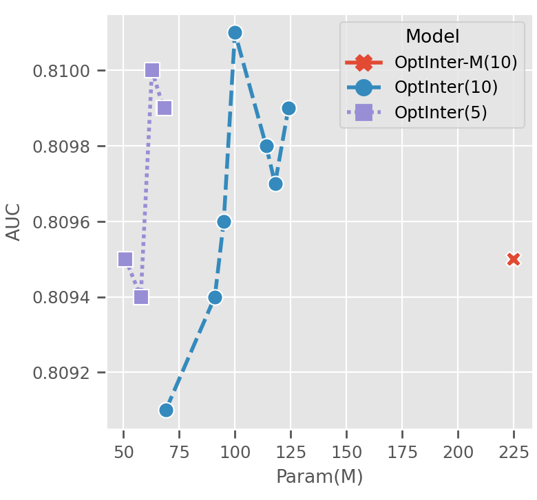
(a) Criteo

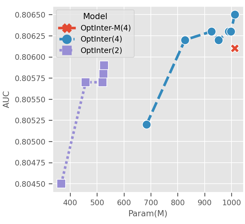
(b) Avazu

Figure 4: Visualization of efficiency-effectiveness trade-off for different datasets. Efficiency is measured by the size of parameters, shown in X-axis. Effectiveness is measured by the AUC score, shown in Y-axis. Here OptInter-M(X) indicates the embedding size of memorized embedding in OptInter-M model being $X$, OptInter(Y) indicates the embedding size of memorized embedding in OptInter model being $Y$.

As demonstrated in Section III-B, OptInter-M is the best baseline. In this section, we further compare OptInter and OptInter-M in terms of effectiveness (measured by AUC) and efficiency (measured by the number of parameters) on Criteo and Avazu datasets. As is shown in Figure 4, three models are compared: OptInter-M(10) sets the embedding size for memorized embeddings to 10, OptInter(10) and OptInter(5) sets the embedding size for memorized embeddings to 10 and 5. In Figure 4(a), AUC varies from 0.8091 to 0.8101 and the number of parameters varies from 50M to 225M. In Figure 4(b), AUC varies from 0.8045 to 0.8065 and the number of parameters varies from 367M to 1012M.

From Figure 4, the following observations can be made. First, OptInter outperforms OptInter-M under many cases with much fewer parameters. This is because OptInter finds suitable and necessary feature interactions to memorize, instead of memorizing all of them as by OptInter-M. Second, the curves of OptInter indicate that its performance degrades dramatically when the number of parameters shrinks below a certain threshold. This reason is that some feature interactions are strong signals that must be memorized to guarantee good performance (some such example feature interactions will be illustrated in Section III-G2). Third, reducing the embedding size for cross-product transformed features can significantly decrease the number of parameters, with only a slight performance drop. This phenomenon suggests that when the space resource is constrained, reducing the embedding size of memorized embeddings is better than throwing away identified feature interactions to be memorized.

III-E Ablation study on the search stage (RQ4)

In this section, we investigate how the search stage affects model performance on public datasets. We compare two search algorithms: Bi-level and OptInter. Bi-level search algorithm updates model parameters and architecture parameters alternatively while the search algorithm in OptInter optimizes these two families of parameters jointly. Bi-level has been widely adopted in neural architecture search domain [16]. However, as discussed in Section II-C, it may be suboptimal to update both model parameters and architecture parameters alternately as a minor updating in architecture parameters leads to a significant change in the model parameters (as also stated in [15]).

TABLE VIII: Comparison between different search algorithm

Dataset	Model	AUC	log loss	Arch	Param.
Criteo	Random	0.8089	0.3764	-	84M
	Bi-level	0.8099	0.3741	[114,109,104]	95M
	OptInter	0.8101	0.3760	[117,98,110]	100M
Avazu	Random	0.8030	0.3658	-	418M
	Bi-level	Out of Memory
	OptInter	0.8062	0.3637	[107,73,96]	827M
iPinYou	Random	0.7781	0.005734	[36,38,46]	108M
	Bi-level	0.7796	0.005620	[34,16,70]	31M
	OptInter	0.7825	0.005606	[25,12,83]	26M

• Arch stands for the searched architecture. [x,y,z] indicates the number of feature interactions that are selected to perform memorized, factorized and naïve methods. Param. represents the number of parameters for this model. Bi-level refers to the result of architectures searched by bi-level optimization. For Random, the mean performance of ten randomly generated architectures are reported here.

As a baseline, we also report the result of performing a random search (namely random). With random search, we randomly assign each feature interaction with one of the three modelling methods. Then the mean values of all the metrics are reported by repeating the random search ten times.

Observed from Table VIII, both two search algorithms, Bi-level and OptInter, outperform randomly generated architecture, which demonstrates the effectiveness of the search stage. The OptInter performs better than Bi-level method, which verifies our previous discussions on how on optimize model parameters and architecture parameters.

Note that Bi-level optimization requires approximate $\sim 2\times$ GPU memory compared with our search algorithm. Therefore, its experiment on the Avazu dataset cannot be accomplished due to the limits of GPU memory.

III-F Ablation study on the re-train stage (RQ4)

In this section, we investigate how the re-train stage affects the model performance. We compare OptInter performance under different settings with and without re-train stage, of which the result is presented in Table IX. It is observed that the re-train stage significantly improves the model performance. Without re-training, the candidate methods to model feature interactions may influence each other, which makes the neural network parameters $\Theta$ suboptimal before the learning process of architecture parameters converges. Re-training makes neural network parameters optimal according to the suitable modelling method for each feature interaction decided in the search stage.

TABLE IX: Performance Comparison between with or without re-train stage

Dataset	Criteo		Avazu
Metric	w.	w.o.	w.	w.o.
AUC	0.8101	0.7953	0.8062	0.7772
log loss	0.3760	0.4558	0.3637	0.3829

• w. stands for re-train stage after search stage with fixed architecture parameters. w.o. stands for without re-train stage after search stage.

These two sub-sections together demonstrate the effectiveness of the two-stage learning algorithm.

III-G Interpretable Discussions (RQ5)

In this section, we investigate which kind of feature interactions are selected by OptInter for each method (namely, memorize, factorize and naïve methods) on Criteo and Avazu. We distinguish feature interactions with mutual information scores between feature interactions and labels. For feature interactions $\{\mathcal{H}=(\mathbf{x}^{o}_{i},\mathbf{x}^{o}_{j})\}$ and ground truth labels $\mathbf{y}$ ($y\in\mathbf{y}$), the mutual information between them is defined as

$$\begin{split}\mathbf{MI}(\mathcal{\{H\}},\mathbf{y})=&-\sum\mathbf{P}(y)\log\mathbf{P}(y)\\ &+\sum\mathbf{P}(\mathcal{H},y)\log\mathbf{P}(y|\mathcal{H}),\end{split}$$ (21)

where the first term is the marginal entropy and the second term is the conditional entropy of ground truth labels $\mathbf{y}$ given feature interaction $\mathcal{H}=(\mathbf{x}^{o}_{i},\mathbf{x}^{o}_{j})$. Note that feature interactions with high mutual information scores are more informative (hence more important) to the prediction.

III-G1 Overall Comparison

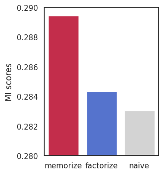
(a) Criteo

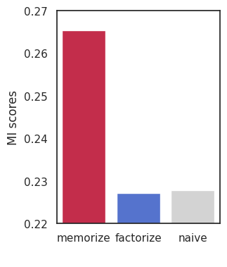
(b) Avazu

Figure 5: Overall mutual information score of each method

We group feature interactions according to each individual method in OptInter. We calculate and compare the mean mutual information scores of the feature interactions modelled by each method, as presented in Figure 5. Three conclusions can be observed. (i) OptInter tends to memorize feature interactions with higher mutual information scores, which is reasonable because treating informative feature interactions as new features makes learning them better. (ii) OptInter removes the feature interactions with low mutual information scores, which helps remove uninformative and noisy feature interactions. (iii) The characteristics of factorized feature interactions in OptInter varies with respect to different datasets. To summarize, the overall trend of feature interactions selected by different methods is consistent with their mutual information scores, which explains the intuition of OptInter. However, it is hard to assign a modelling method to each feature interaction based on heuristics as it may not be optimal, which motivates an automatic framework to do so.

III-G2 Case Study

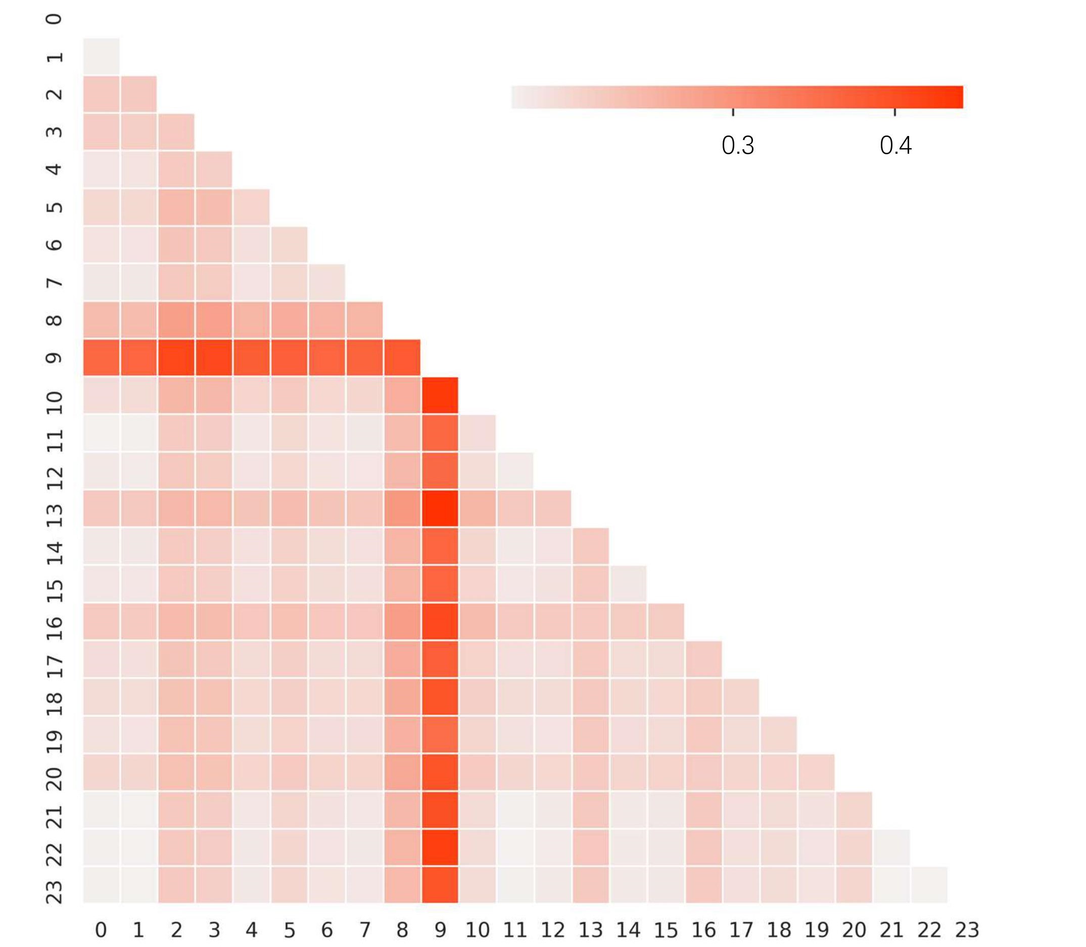
(a) Heatmap of mutual information between each feature interaction and the label

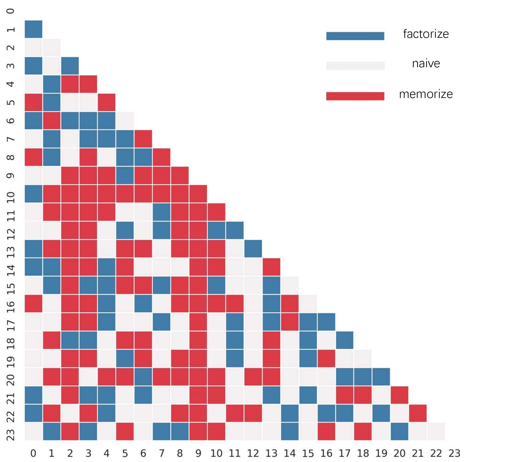
(b) Obtained optimal methods for feature interactions

Figure 6: An example of interpretability on Avazu Dataset. In both subfigures, the number indicates the field ID. In subfigure (a), the color indicates the strength of feature interaction in predicting label. In subfigure (b), different colors indicate three modelling methods searched by OptInter.

As a case study, we investigate the selected method for each feature interaction OptInter method on the Avazu dataset, which is shown in Figure 6. Figure 6(a) shows the heat map of mutual information scores of all the feature interactions, which represents how informative each feature interaction is in predicting the label. Figure 6(b) shows the searched method for each feature interaction. As can be seen, these two maps are positively correlated to each other, which indicates that OptInter obtains the optimal method for each feature interaction.

IV Related Work

IV-A Feature Interaction in CTR Prediction

Feature interaction is one of the core problems in CTR prediction [5, 3, 4, 2, 18, 15, 14]. Feature interaction is one of the core problems in CTR prediction [5, 3, 4, 2, 18, 15, 14]. Generalized linear models like Logistic Regression (LR) [24, 27] model feature interaction naively, i.e., they do not model feature interactions. One way to model all feature interactions is based on degree-2 polynomial mappings[8]. It increases model performance, but it also leads to a combinatorial explosion. One possible solution is to design feature interactions manually. However, this requires experts’ experience and is hard to generalize. Other methods like FM [9] and its variants [11, 10] models the low order feature interactions by factorizing them with latent vectors.

With the success of deep learning in computer vision and natural language processes, the deep CTR prediction model has gained tremendous attention in recent years. Compared with the linear model, deep models can predict CTR more effectively. Usually, deep CTR models choose to model feature interaction into three classes: naïve [5], memorized [1], and factorized [3, 4, 2]. FNN [5], as an example of naïve modelling, introduces multi-layer perceptron to predict CTR scores with original features. However, such modelling method usually leads to lower model capacity (compared to the other two methods) because it cannot learn low-rank feature interactions well [7].

Memorized methods model feature interaction by memorizing them explicitly as new features. Wide&Deep [1], as an example, indicates that the memorized method is a promising alternative for strong feature interactions. More specifically, Wide&Deep [1] memorizes a manually selected set of feature interactions and feeds it into its wide component. In the experiments of [1], the model structure for Google Play selects the feature interaction (User_Installed_App, Impression_App) as new feature for its wide component. This is a powerful indicator for a user downloading an app, as the installation history indicates user preference. However, this requires experts’ experience and is hard to generalize. Moreover, memorized method induces a severe feature sparsity problem because the occurrence of many new features (generated by feature interactions) is relatively less than original features in the training set. The severe feature sparsity problem makes these infrequent new features difficult to learn and degrades the model performance.

Due to this reason, factorized methods are proposed to model feature interactions via a factorization function. Mainstream deep CTR models [2, 3, 4] usually adopt factorized method to model feature interactions. For example, IPNN and OPNN [3] use inner-product and outer-product as the factorization function, respectively. DeepFM [2] borrows the FM layer from Factorization Machine [9] and uses that as a factorization function. PIN [4], improving on IPNN and OPNN [3], uses a small MLP component to model as a learnable factorization function. Factorized methods alleviate feature sparsity issue as they assign learnable parameters to original features instead of assigning them to new features (generated by feature interactions) with a much larger feature space. However, these methods have their inherited drawbacks. As the feature interactions are modelled by the latent vectors of original features, the latent vectors take the responsibility of both representation learning and feature interaction modelling. These two tasks may conflict with each other so that the model performance is bounded, as observed in [13, 14].

Recently CAN [14] highlights the importance of memorized method. It manually selects a subset of feature interactions to memorize and prove its effectiveness through extensive experiments. But their model design still makes CAN be a factorized method.

OptInter is the first work introducing the memorized method in deep CTR models (although Wide&Deep uses memorized method, it applies memorized method to its wide component only). Furthermore, OptInter is general enough to unify mainstream deep CTR models under its framework.

IV-B Neural architecture search (NAS) and its application in Recommender System

Neural architecture search (NAS) aims at automatically finding an optimal architecture for specific tasks and datasets, which avoids manual design [28, 29, 16, 30, 17, 31]. These methods could be used to find optimal network structures, loss functions or hyper-parameters, significantly reducing human intervention in the ML pipeline. These methods can be categorized into three classes: (i) reinforcement learning-based methods [28, 29] train an external controller (like RNN or reinforcement learning agent) to design cell structure for a specific model architecture; (ii) evolutionary algorithms [17, 31] that try to evolve an optimal architecture by mutating the top-$k$ architectures and explore new potential models; (iii) gradient-based methods [30, 16] relax the search space to be continuous instead of searching on a discrete set of architectures. Such relaxation allows the searching process to be more efficient based on a gradient descent optimizer.

Recently, NAS methods have attracted much attention in the CTR prediction task. AutoFIS [15] utilizes GRDA Optimizer [25] to select proper feature interactions. AutoFeature [18] adopts a tree of Naive Bayes classifiers to find suitable feature interaction functions for various fields. AutoPI [20] extends the search space to computational graph and feature interaction functions to achieve higher generalization. Many research works [32, 33, 34] aim to select suitable dimensions for various fields. AutoDis [35] focuses on modelling continuous feature and proposes a framework to select optimal discretization methods. AutoFT [36] proposes an end-to-end transfer learning framework to automatically determine transfer policy in CTR prediction via Gumbel-softmax tricks [19]. AutoLoss [37] proposes a framework that learn sample-specific loss function via bi-level optimization.

OptInter has its uniqueness compared with other research works that apply NAS techniques into the CTR prediction task. Compared with the works which focus on modelling feature interaction [15, 18, 20], OptInter introduces memorized methods into its search space and searches within a broader space than existing works.

V Conclusion

In this paper, we proposed a novel deep CTR prediction framework named OptInter, which is the first to introduce the memorized feature interaction method in deep CTR models. OptInter can search and identify the optimal method to model the feature interactions from naïve, memorized and factorized. To achieve this, we first proposed a deep framework that unifies mainstream deep CTR models. Then, as a part of OptInter, a two-stage learning algorithm is proposed. In the search stage, the search process is modelled as an architecture search problem solved efficiently by neural architecture search techniques. During the re-train stage, the model is re-trained from scratch to achieve better performance. Extensive experiments on four large-scale datasets demonstrate the superior performance of OptInter. Several ablation studies show our method is effective in improving prediction performance and efficient in model size. Moreover, we also explain obtained results in the view of mutual information, which further highlights our method learns the optimal feature interaction methods.

References

- [1] H. Cheng, L. Koc, J. Harmsen, T. Shaked, T. Chandra, H. Aradhye, G. Anderson, G. Corrado, W. Chai, M. Ispir, R. Anil, Z. Haque, L. Hong, V. Jain, X. Liu, and H. Shah, “Wide & deep learning for recommender systems,” in Proceedings of the 1st Workshop on Deep Learning for Recommender Systems, DLRS@RecSys 2016, Boston, MA, USA, September 15, 2016, A. Karatzoglou, B. Hidasi, D. Tikk, O. S. Shalom, H. Roitman, B. Shapira, and L. Rokach, Eds. ACM, 2016, pp. 7–10.
- [2] H. Guo, R. Tang, Y. Ye, Z. Li, and X. He, “Deepfm: A factorization-machine based neural network for CTR prediction,” in Proceedings of the Twenty-Sixth International Joint Conference on Artificial Intelligence, IJCAI 2017, Melbourne, Australia, August 19-25, 2017, C. Sierra, Ed. ijcai.org, 2017, pp. 1725–1731.
- [3] Y. Qu, H. Cai, K. Ren, W. Zhang, Y. Yu, Y. Wen, and J. Wang, “Product-based neural networks for user response prediction,” in IEEE 16th International Conference on Data Mining, ICDM 2016, December 12-15, 2016, Barcelona, Spain, F. Bonchi, J. Domingo-Ferrer, R. Baeza-Yates, Z. Zhou, and X. Wu, Eds. IEEE Computer Society, 2016, pp. 1149–1154.
- [4] Y. Qu, B. Fang, W. Zhang, R. Tang, M. Niu, H. Guo, Y. Yu, and X. He, “Product-based neural networks for user response prediction over multi-field categorical data,” ACM Trans. Inf. Syst., vol. 37, no. 1, pp. 5:1–5:35, 2019.
- [5] W. Zhang, T. Du, and J. Wang, “Deep learning over multi-field categorical data - - A case study on user response prediction,” in Advances in Information Retrieval - 38th European Conference on IR Research, ECIR 2016, Padua, Italy, March 20-23, 2016. Proceedings, ser. Lecture Notes in Computer Science, N. Ferro, F. Crestani, M. Moens, J. Mothe, F. Silvestri, G. M. D. Nunzio, C. Hauff, and G. Silvello, Eds., vol. 9626. Springer, 2016, pp. 45–57.
- [6] K. Hornik, M. B. Stinchcombe, and H. White, “Multilayer feedforward networks are universal approximators,” Neural Networks, vol. 2, no. 5, pp. 359–366, 1989.
- [7] A. Beutel, P. Covington, S. Jain, C. Xu, J. Li, V. Gatto, and E. H. Chi, “Latent cross: Making use of context in recurrent recommender systems,” in Proceedings of the Eleventh ACM International Conference on Web Search and Data Mining, WSDM 2018, Marina Del Rey, CA, USA, February 5-9, 2018, Y. Chang, C. Zhai, Y. Liu, and Y. Maarek, Eds. ACM, 2018, pp. 46–54.
- [8] Y. Chang, C. Hsieh, K. Chang, M. Ringgaard, and C. Lin, “Training and testing low-degree polynomial data mappings via linear SVM,” J. Mach. Learn. Res., vol. 11, pp. 1471–1490, 2010.
- [9] S. Rendle, “Factorization machines,” in ICDM 2010, The 10th IEEE International Conference on Data Mining, Sydney, Australia, 14-17 December 2010, G. I. Webb, B. Liu, C. Zhang, D. Gunopulos, and X. Wu, Eds. IEEE Computer Society, 2010, pp. 995–1000.
- [10] Y. Juan, Y. Zhuang, W. Chin, and C. Lin, “Field-aware factorization machines for CTR prediction,” in Proceedings of the 10th ACM Conference on Recommender Systems, Boston, MA, USA, September 15-19, 2016, S. Sen, W. Geyer, J. Freyne, and P. Castells, Eds. ACM, 2016, pp. 43–50.
- [11] J. Pan, J. Xu, A. L. Ruiz, W. Zhao, S. Pan, Y. Sun, and Q. Lu, “Field-weighted factorization machines for click-through rate prediction in display advertising,” in Proceedings of the 2018 World Wide Web Conference on World Wide Web, WWW 2018, Lyon, France, April 23-27, 2018, P. Champin, F. Gandon, M. Lalmas, and P. G. Ipeirotis, Eds. ACM, 2018, pp. 1349–1357.
- [12] Y. Sun, J. Pan, A. Zhang, and A. Flores, “Fm: Field-matrixed factorization machines for recommender systems,” CoRR, vol. abs/2102.12994, 2021.
- [13] S. Prillo, “An elementary view on factorization machines,” in Proceedings of the Eleventh ACM Conference on Recommender Systems, RecSys 2017, Como, Italy, August 27-31, 2017, P. Cremonesi, F. Ricci, S. Berkovsky, and A. Tuzhilin, Eds. ACM, 2017, pp. 179–183.
- [14] G. Zhou, W. Bian, K. Wu, L. Ren, Q. Pi, Y. Zhang, C. Xiao, X. Sheng, N. Mou, X. Luo, C. Zhang, X. Qiao, S. Xiang, K. Gai, X. Zhu, and J. Xu, “CAN: revisiting feature co-action for click-through rate prediction,” CoRR, vol. abs/2011.05625, 2020.
- [15] B. Liu, C. Zhu, G. Li, W. Zhang, J. Lai, R. Tang, X. He, Z. Li, and Y. Yu, “Autofis: Automatic feature interaction selection in factorization models for click-through rate prediction,” in KDD ’20: The 26th ACM SIGKDD Conference on Knowledge Discovery and Data Mining, Virtual Event, CA, USA, August 23-27, 2020, R. Gupta, Y. Liu, J. Tang, and B. A. Prakash, Eds. ACM, 2020, pp. 2636–2645.
- [16] H. Liu, K. Simonyan, and Y. Yang, “DARTS: differentiable architecture search,” CoRR, vol. abs/1806.09055, 2018.
- [17] E. Real, S. Moore, A. Selle, S. Saxena, Y. L. Suematsu, J. Tan, Q. V. Le, and A. Kurakin, “Large-scale evolution of image classifiers,” in Proceedings of the 34th International Conference on Machine Learning, ICML 2017, Sydney, NSW, Australia, 6-11 August 2017, ser. Proceedings of Machine Learning Research, D. Precup and Y. W. Teh, Eds., vol. 70. PMLR, 2017, pp. 2902–2911.
- [18] F. Khawar, X. Hang, R. Tang, B. Liu, Z. Li, and X. He, “Autofeature: Searching for feature interactions and their architectures for click-through rate prediction,” in CIKM ’20: The 29th ACM International Conference on Information and Knowledge Management, Virtual Event, Ireland, October 19-23, 2020, M. d’Aquin, S. Dietze, C. Hauff, E. Curry, and P. Cudré-Mauroux, Eds. ACM, 2020, pp. 625–634.
- [19] E. Jang, S. Gu, and B. Poole, “Categorical reparameterization with gumbel-softmax,” in 5th International Conference on Learning Representations, ICLR 2017, Toulon, France, April 24-26, 2017, Conference Track Proceedings. OpenReview.net, 2017.
- [20] Z. Meng, J. Zhang, Y. Li, J. Li, T. Zhu, and L. Sun, “A general method for automatic discovery of powerful interactions in click-through rate prediction,” CoRR, vol. abs/2105.10484, 2021.
- [21] Y. Xie, Z. Wang, Y. Li, B. Ding, N. M. Gürel, C. Zhang, M. Huang, W. Lin, and J. Zhou, “Interactive feature generation via learning adjacency tensor of feature graph,” CoRR, vol. abs/2007.14573, 2020.
- [22] L. J. Ba, J. R. Kiros, and G. E. Hinton, “Layer normalization,” CoRR, vol. abs/1607.06450, 2016.
- [23] E. J. Gumbel, “Categorical reparameterization with gumbel-softmax,” in Statistical theory of extreme values and some practical applications: a series of lectures, Vol. 33, US. US Government Printing Office, 1945.
- [24] M. Richardson, E. Dominowska, and R. Ragno, “Predicting clicks: estimating the click-through rate for new ads,” in Proceedings of the 16th International Conference on World Wide Web, WWW 2007, Banff, Alberta, Canada, May 8-12, 2007, C. L. Williamson, M. E. Zurko, P. F. Patel-Schneider, and P. J. Shenoy, Eds. ACM, 2007, pp. 521–530.
- [25] S. Chao, Z. Wang, Y. Xing, and G. Cheng, “Directional pruning of deep neural networks,” in Advances in Neural Information Processing Systems 33: Annual Conference on Neural Information Processing Systems 2020, NeurIPS 2020, December 6-12, 2020, virtual, H. Larochelle, M. Ranzato, R. Hadsell, M. Balcan, and H. Lin, Eds., 2020.
- [26] X. Glorot and Y. Bengio, “Understanding the difficulty of training deep feedforward neural networks,” in Proceedings of the Thirteenth International Conference on Artificial Intelligence and Statistics, AISTATS 2010, Chia Laguna Resort, Sardinia, Italy, May 13-15, 2010, ser. JMLR Proceedings, Y. W. Teh and D. M. Titterington, Eds., vol. 9. JMLR.org, 2010, pp. 249–256.
- [27] X. He, J. Pan, O. Jin, T. Xu, B. Liu, T. Xu, Y. Shi, A. Atallah, R. Herbrich, S. Bowers, and J. Q. Candela, “Practical lessons from predicting clicks on ads at facebook,” in Proceedings of the Eighth International Workshop on Data Mining for Online Advertising, ADKDD 2014, August 24, 2014, New York City, New York, USA, E. Saka, D. Shen, K. Lee, and Y. Li, Eds. ACM, 2014, pp. 5:1–5:9.
- [28] B. Baker, O. Gupta, N. Naik, and R. Raskar, “Designing neural network architectures using reinforcement learning,” in 5th International Conference on Learning Representations, ICLR 2017, Toulon, France, April 24-26, 2017, Conference Track Proceedings. OpenReview.net, 2017.
- [29] B. Zoph and Q. V. Le, “Neural architecture search with reinforcement learning,” in 5th International Conference on Learning Representations, ICLR 2017, Toulon, France, April 24-26, 2017, Conference Track Proceedings. OpenReview.net, 2017.
- [30] R. Luo, F. Tian, T. Qin, E. Chen, and T. Liu, “Neural architecture optimization,” in Advances in Neural Information Processing Systems 31: Annual Conference on Neural Information Processing Systems 2018, NeurIPS 2018, December 3-8, 2018, Montréal, Canada, S. Bengio, H. M. Wallach, H. Larochelle, K. Grauman, N. Cesa-Bianchi, and R. Garnett, Eds., 2018, pp. 7827–7838.
- [31] E. Real, A. Aggarwal, Y. Huang, and Q. V. Le, “Regularized evolution for image classifier architecture search,” in The Thirty-Third AAAI Conference on Artificial Intelligence, AAAI 2019, The Thirty-First Innovative Applications of Artificial Intelligence Conference, IAAI 2019, The Ninth AAAI Symposium on Educational Advances in Artificial Intelligence, EAAI 2019, Honolulu, Hawaii, USA, January 27 - February 1, 2019. AAAI Press, 2019, pp. 4780–4789.
- [32] X. Zhao, H. Liu, H. Liu, J. Tang, W. Guo, J. Shi, S. Wang, H. Gao, and B. Long, “Memory-efficient embedding for recommendations,” CoRR, vol. abs/2006.14827, 2020.
- [33] X. Zhao, C. Wang, M. Chen, X. Zheng, X. Liu, and J. Tang, “Autoemb: Automated embedding dimensionality search in streaming recommendations,” CoRR, vol. abs/2002.11252, 2020.
- [34] H. Liu, X. Zhao, C. Wang, X. Liu, and J. Tang, “Automated embedding size search in deep recommender systems,” in Proceedings of the 43rd International ACM SIGIR conference on research and development in Information Retrieval, SIGIR 2020, Virtual Event, China, July 25-30, 2020, J. Huang, Y. Chang, X. Cheng, J. Kamps, V. Murdock, J. Wen, and Y. Liu, Eds. ACM, 2020, pp. 2307–2316.
- [35] H. Guo, B. Chen, R. Tang, Z. Li, and X. He, “Autodis: Automatic discretization for embedding numerical features in CTR prediction,” CoRR, vol. abs/2012.08986, 2020.
- [36] X. Yang, Q. Liu, R. Su, R. Tang, Z. Liu, and X. He, “Autoft: Automatic fine-tune for parameters transfer learning in click-through rate prediction,” CoRR, vol. abs/2106.04873, 2021.
- [37] X. Zhao, H. Liu, W. Fan, H. Liu, J. Tang, and C. Wang, “Autoloss: Automated loss function search in recommendations,” CoRR, vol. abs/2106.06713, 2021.