Exposing minimal composition of Kohn-Sham theory and its extendability

Abstract

Reducing the many-fermion problem to a set of single-particle (s.p.) equations, the Kohn-Sham (KS) theory has provided a practical tool to implement ab initio calculations of ground-state energies and densities in many-electron systems. There have been attempts to extend the KS theory so that it could describe other physical quantities, or it could be applied to other many-fermion systems. By generalizing and reformulating the KS theory in terms of the 1-body density matrix, we expose the minimal composition of the theory that enables the reduction of the many-fermion problem to the s.p. equations. Based on the reformulation, several basic issues are reconsidered. The $v$- and $N$-representabilities for the KS theory are distinguished from those for the Hohenberg-Kohn theorem. Criteria for the extendability of the KS theory are addressed.

I Introduction

The density-functional theory (DFT) successfully described many-electron systems ranging from atoms and molecules to solids Parr and Yang (1989); Giuliani and Vignale (2005); Engel and Dreizler (2011); Sahni (2016), in which the influence of the ions is handled as external fields via the Born-Oppenheimer approximation. Located at its center, the Hohenberg-Kohn (HK) theorem Hohenberg and Kohn (1964) has provided the firm basis of the DFT, and the Kohn-Sham (KS) theory Kohn and Sham (1965) has made the DFT practical for electronic systems. They have supplied an ab initio theory for ground-state (g.s.) energy $E_{0}$. The energy of system $E$ is represented as a functional of the local density $n(\mathbf{r})$, and $E_{0}$ is obtained via the variation of the energy density functional (EDF).

The KS theory has been attempted to be extended in various directions. In electronic systems, the EDFs including variables additional to $n(\mathbf{r})$ were developed: for instance, the spin DFT von Barth and Hedin (1972); Gunnarsson and Lundqvist (1976); Jacob and Reiher (2012), the current DFT Vignale and Rasolt (1987, 1988), the DFT for superconductors Oliveira et al. (1988); Lüders et al. (2005), and the density-matrix functional theory Donnely and Parr (1978); Zumbach and Maschke (1985); Schindlmayr and Godby (1995); López-Sandoval and Pastor (2000); Requistl and Pankratov (2008); Pernal and Giesbertz (2016). A systematic method to involve additional quantities has been proposed Higuchi and Higuchi (2004). The DFT has also been extended to finite-temperature problems Mermin (1965) and to excitations via a time-dependent formalism Runge and Gross (1984); Gross and Kohn (1985), although we focus on the g.s. properties in this paper. Another direction is to extend the KS theory to other many-fermion systems. For atomic nuclei composed of nucleons, the self-consistent mean-field (SCMF) calculations have been implemented Vautherin and Brink (1972) by using effective interactions in which correlation effects are incorporated. The most popular form of effective interactions is the Skyrme interaction Skyrme (1959), representing energy via quasi-local currents, i.e., currents that depend only on a position $\mathbf{r}$, by attributing influences of non-locality to momentum-dependence. These SCMF approaches have been reinterpreted in the context of the DFT Petkov and Stoitsov (1991); Colò (2020). Calculations using finite-range effective interactions, which lead to non-local EDFs, have been developed as well Dechargé and Gogny (1980); Nakada (2003). The SCMF approaches incorporating relativity Serot and Walecka (1986) are also renamed the covariant DFT Ring (2016).

The KS theory’s remarkable and essential property is that the many-fermion problem is reduced to a set of single-particle (s.p.) equations. In this paper, we shall generalize and reformulate the KS theory, aiming to expose the minimal composition of the theory, i.e., with what ingredients at minimum the many-fermion problem can be solved by s.p. equations. Through the reformulation, criteria for the extendability of the theory will be elucidated. They help to judge what physical quantities can be covered by extending it and to what system it can be extended.

The so-called orbital-free (OF) DFT, which has a root in the historical work by Thomas and Fermi Thomas (1927); Fermi (1928), has been developed Deb and Chattaraj (1988, 1992); Pearson et al. (1993) to reduce the computational cost further. Whereas the OF DFT is often considered an approximation of the KS DFT, it does not need s.p. equations and should be distinguished from the KS theory in this respect. As one of our central issues is the emergence of the s.p. equations, we will not handle the OF DFT in this paper, except for a brief referral.

We restrict our discussion to systems where the particle number $N$ is conserved. An arbitrary normalized state in the system is represented by $|\Psi\rangle$. Denoting the Hamiltonian of this system by $H$, the energy expectation value is regarded as a functional of $|\Psi\rangle$,

$$E[\Psi]:=\langle\Psi|H|\Psi\rangle\,.$$ (1)

The variational principle tells us that $E_{0}$ is equal to the minimum of $E[\Psi]$ with respect to $|\Psi\rangle$,

$$E_{0}=\min_{\Psi\to N}E[\Psi]\,,$$ (2)

where the subscript $\Psi\to N$ stands for the condition that the state $|\Psi\rangle$ should belong to the $N$-particle system. However, the underlying Hamiltonian is not well established in certain systems; the atomic nuclei are among them. For this reason, $E[\Psi]$ and the variational principle (2) are placed at the starting point in the arguments below, not necessarily presuming $H$. Moreover, we shall present the formulation in terms of the 1-body density matrix, which carries properties of $|\Psi\rangle$. While $n(\mathbf{r})$ is adopted as the principal variable for the variation in the original HK theorem, we merely assume that the principal variables are all s.p. quantities, viz., functions of the 1-body density matrix, not restricting to $n(\mathbf{r})$.

II Hartree-Fock approximation

The KS theory significantly overlaps with the SCMF approximations. Both approaches reduce many-fermion problems to a set of s.p. equations. In this section we review the Hartree-Fock (HF) approximation, which is a typical and rigorous example of the SCMF theories, in terms of the 1-body density matrix Ring and Schuck (1980). The arguments here will clarify the basic structure of the SCMF theories, which is possessed by the KS theory as well. Another example, the Hartree-Fock-Bogolyubov (HFB) approximation, is summarized in Appendix A.

Let $\{\phi_{k}\}$ represent a complete orthonormal set of s.p. bases. The creation and annihilation operators of the basis state $k$ are denoted by $a^{\dagger}_{k}$ and $a_{k}$. The 1-body density matrix $\varrho_{k\ell}$ for an arbitrary normalized state $|\Psi\rangle$ is defined by

$$\varrho_{k\ell}=\varrho_{k\ell}[\Psi]:=\langle\Psi|a^{\dagger}_{\ell}a_{k}|\Psi\rangle=\varrho_{\ell k}^{\ast}\,.$$ (3)

The $\nu$-body density matrix $\langle\Psi|a^{\dagger}_{\ell_{1}}a^{\dagger}_{\ell_{2}}\cdots a^{\dagger}_{\ell_{\nu}}a_{k_{\nu}}\cdots a_{k_{2}}a_{k_{1}}|\Psi\rangle$ is decomposed into products of $\varrho_{k\ell}$ and the correlation functions $\mathcal{C}^{(\nu^{\prime})}$ ($\nu^{\prime}=2,3,\cdots,\nu$), which obey the Bogolyubov-Born-Green-Kirkwood-Yvon hierarchy Reichl (1980). For instance, the 2-body correlation function is defined by

$$\mathcal{C}^{(2)}_{kk^{\prime}\ell\ell^{\prime}}:=\langle\Psi|a^{\dagger}_{\ell}a^{\dagger}_{\ell^{\prime}}a_{k^{\prime}}a_{k}|\Psi\rangle-\varrho_{k\ell}\varrho_{k^{\prime}\ell^{\prime}}+\varrho_{k\ell^{\prime}}\varrho_{\ell k^{\prime}}\,.$$ (4)

$E[\Psi]$ can be represented by $\varrho$ and $\mathcal{C}^{(\nu)}$,

$$E[\Psi]=E[\varrho,\mathcal{C}^{(2)},\mathcal{C}^{(3)},\cdots,\mathcal{C}^{(N)}]\,.$$ (5)

By neglecting $\mathcal{C}^{(\nu)}$ ($\nu\geq 2$), the energy functional in the HF approximation is obtained, $E[\Psi]\approx E^{\mathrm{HF}}[\varrho]$. Variation of $E^{\mathrm{HF}}[\varrho]$ for $\varrho_{k\ell}$ yields a s.p. Hamiltonian (HF Hamiltonian),

$$h^{\mathrm{HF}}_{k\ell}:=\frac{\partial E^{\mathrm{HF}}}{\partial\varrho_{\ell k}}=\big{(}h^{\mathrm{HF}}_{\ell k}\big{)}^{\ast}\,.$$ (6)

The diagonalization of $h^{\mathrm{HF}}$ with an appropriate unitary transformation $\mathcal{U}^{\mathrm{HF}}$ yields

$$\sum_{\ell}h^{\mathrm{HF}}_{k\ell}\,\mathcal{U}^{\mathrm{HF}}_{\ell i}=\epsilon^{\mathrm{HF}}_{i}\,\mathcal{U}^{\mathrm{HF}}_{ki}\,,$$ (7)

which is identical to the HF equation, determining s.p. energy $\epsilon^{\mathrm{HF}}_{i}$ and wave-function $\varphi^{\mathrm{HF}}_{i}=\sum_{k}\mathcal{U}^{\mathrm{HF}}_{ki}\,\phi_{k}$.

The HF state $|\Phi^{\mathrm{HF}}\rangle$ is obtained by minimizing $E^{\mathrm{HF}}$ with respect to $\varrho_{k\ell}$ under the particle-number condition,

$$\mathrm{tr}(\varrho)=N\,.$$ (8)

The trace in Eq. (8) is taken in the s.p. space. To implement the minimization, Eq. (8) is handled with the Lagrange multiplier $\mu$, modifying $E^{\mathrm{HF}}$ as

$$\tilde{E}^{\mathrm{HF}}:=E^{\mathrm{HF}}-\mu\big{[}\mathrm{tr}(\varrho)-N\big{]}\,.$$ (9)

Variation of $\tilde{E}^{\mathrm{HF}}$ yields

$$\begin{split}\delta\tilde{E}^{\mathrm{HF}}&=\sum_{k\ell}\frac{\partial E^{\mathrm{HF}}}{\partial\varrho_{\ell k}}\,\delta\varrho_{\ell k}-\mu\sum_{k}\delta\varrho_{kk}-\delta\mu\big{[}\mathrm{tr}(\varrho)-N\big{]}\\ &=\mathrm{tr}\big{[}(h^{\mathrm{HF}}-\mu)\,\delta\varrho\big{]}-\delta\mu\big{[}\mathrm{tr}(\varrho)-N\big{]}\,.\end{split}$$ (10)

We should have $\delta\tilde{E}^{\mathrm{HF}}\geq 0$ at the minimum of $E^{\mathrm{HF}}$.

The Pauli principle requires

$$0\leq\varrho_{ii}\leq 1\quad\mbox{for any representation}\,.$$ (11)

By combining $\delta\tilde{E}^{\mathrm{HF}}\geq 0$ with Eq. (11), it is concluded that $|\Phi^{\mathrm{HF}}\rangle$ should be a state corresponding to a single Slater determinant, as proven below. In $\delta\tilde{E}^{\mathrm{HF}}$ of Eq. (10), the $\delta\mu$ term vanishes as long as Eq. (8) is fulfilled. Suppose that $\{\varrho^{\mathrm{HF}}_{k\ell}\,(:=\varrho_{k\ell}[\Phi^{\mathrm{HF}}])\}$ gives the minimum of $E^{\mathrm{HF}}$ under the constraint (8), which is equal to the minimum of $\tilde{E}^{\mathrm{HF}}$. The s.p. energy $\epsilon^{\mathrm{HF}}_{i}$ and wave-function $\varphi^{\mathrm{HF}}_{i}$ are determined accordingly. It is convenient to work with the s.p. state $i$ instead of the basis $k$ in the vicinity of the HF solution. In this vicinity, Eq. (10) is expressed as

$$\delta\tilde{E}^{\mathrm{HF}}=\sum_{i}(\epsilon^{\mathrm{HF}}_{i}-\mu)\,\delta\varrho_{ii}\,.$$ (12)

The requirement $\delta\tilde{E}^{\mathrm{HF}}\geq 0$ at the minimum of $E^{\mathrm{HF}}$ derives

$$\left\{\begin{array}[]{ll}\delta\varrho_{ii}\geq 0&\mbox{for $i$ with }\epsilon^{\mathrm{HF}}_{i}>\mu\\ \delta\varrho_{ii}\leq 0&\mbox{for $i$ with }\epsilon^{\mathrm{HF}}_{i}<\mu\end{array}\right.\,.$$ (13)

Combined with (11), Eq. (13) leads to

$$\left\{\begin{array}[]{ll}\varrho^{\mathrm{HF}}_{ii}=0&\mbox{for $i$ with }\epsilon^{\mathrm{HF}}_{i}>\mu\\ \varrho^{\mathrm{HF}}_{ii}=1&\mbox{for $i$ with }\epsilon^{\mathrm{HF}}_{i}<\mu\end{array}\right.\,,$$ (14)

so that negative $\delta\varrho_{ii}$ should not be allowed for $\epsilon^{\mathrm{HF}}_{i}>\mu$ and likewise for $\epsilon^{\mathrm{HF}}_{i}<\mu$. Since $\varrho_{ii}$ is the occupation number on the s.p. state $i$, the lowest $N$ s.p. states are occupied in $|\Phi^{\mathrm{HF}}\rangle$ unless there exist s.p. levels with $\epsilon^{\mathrm{HF}}_{i}=\mu$, which could be degenerate. Even if there are several levels having $\epsilon^{\mathrm{HF}}_{i}=\mu$, the occupation number on them can be set integer, viz., $0$ or $1$, through a unitary transformation among the degenerate s.p. states. Therefore $|\Phi^{\mathrm{HF}}\rangle$ can be represented by a single Slater determinant, which is formed by $\{\varphi^{\mathrm{HF}}_{i}\}$ with $\varrho^{\mathrm{HF}}_{ii}=1$. As the $\epsilon^{\mathrm{HF}}_{i}=\mu$ levels do not influence essential points but make arguments lengthy, we shall assume $\epsilon^{\mathrm{HF}}_{i}\neq\mu$ for any $i$ below.

Because of Condition (11), $\varrho^{\mathrm{HF}}_{ii}$ of Eq. (14) has reached either its maximum or minimum that can be obtained by any unitary transformation, implying that $\varrho^{\mathrm{HF}}$ is diagonalized in this representation. When its eigenvalues are only $0$ and $1$, the density matrix $\varrho$ is characterized by the idempotency,

$$\varrho^{2}=\varrho\,,\quad\mbox{viz.,}\quad\sum_{m}\varrho_{km}\,\varrho_{m\ell}=\varrho_{k\ell}\,.$$ (15)

A state given by a single Slater determinant $|\Phi\rangle$ provides $\varrho_{k\ell}=\langle\Phi|a^{\dagger}_{\ell}a_{k}|\Phi\rangle$ that fulfills Eq. (15), as is evident by representing it through the s.p. states $\{\varphi_{i};i=1,2,\cdots,N\}$ forming $|\Phi\rangle$. Conversely, if $\{\varrho_{k\ell}\}$ satisfies Eq. (15), the corresponding state is given by a Slater determinant. This assertion is easily proven by constructing the Slater determinant: take the s.p. states $\{\varphi_{i}\}$ that diagonalize $\varrho$ and pick up the states corresponding to the eigenvalue $1$. Thus, $\varrho^{\mathrm{HF}}$ satisfying Eq. (15) and $|\Phi^{\mathrm{HF}}\rangle$ is represented by a single Slater determinant. Let us denote the full Hilbert space of the $N$-particle system by $\mathcal{V}_{\mathrm{full}}$, and the subspace composed of the states of the Slater determinants by $\mathcal{V}_{\mathrm{idem}}$, which are characterized by Eq. (15). It is noted that, although $E^{\mathrm{HF}}[\varrho]$ is defined in $\mathcal{V}_{\mathrm{full}}$, the wave-function necessarily falls on $\mathcal{V}_{\mathrm{idem}}$, as the result of the variation. This fact is equivalent to the conclusion in Ref. Lieb (1981).

III Hohenberg-Kohn theorem

We present the Hohenberg-Kohn (HK) theorem in this section. Whereas it is no more than a summary of many previous works, we state and discuss the HK theorem in a generalized context, preparing to reformulate the KS theory.

Consider a set of variables $Q^{A}$, which are called principal variables in this article. The superscript $A$ distinguishes the variables, which can be continuous. For brevity, the set of $Q^{A}$ is denoted by $\mathbf{Q}$. In the original HK theorem Hohenberg and Kohn (1964), $\mathbf{Q}$ is the local density $n(\mathbf{r}):=\langle\Psi|\sum_{i=1}^{N}\delta(\mathbf{r}-\mathbf{r}_{i})|\Psi\rangle$, where $i$ is the index of particles. As mentioned in Introduction, additional variables have been introduced in $\mathbf{Q}$ when extending the DFT. In Ref. Gilbert (1975), the HK theorem has extensively been proven for the whole 1-body density matrix, $\mathbf{Q}=\{\varrho_{k\ell}\}$.

The HK theorem (the so-called 2nd theorem) asserts the existence of the functional $E^{\mathrm{HK}}[\mathbf{Q}]$, whose minimum gives exact g.s. energy and corresponding $\mathbf{Q}$. The theorem was initially proven by showing the one-to-one correspondence of $\mathbf{Q}=n(\mathbf{r})$ and the external potential (the 1st HK theorem), which is equivalent to the Legendre transformation. The Legendre transformation was also applied in the effective action formalism, deriving the HK theorem in an elegant manner Fukuda et al. (1994); Valiev and Fernando (1997). However, we follow Levy’s idea of the constrained search Levy (1979), which derives a universal energy functional of $\mathbf{Q}$ and provides a basis for the KS theory. The HK energy functional can be defined by

$$E^{\mathrm{HK}}[\mathbf{Q}]:=\min_{\Psi\to\mathbf{Q}}E[\Psi]\,.$$ (16)

Here the expression $\Psi\to\mathbf{Q}$ indicates the constraint that $|\Psi\rangle$ gives a fixed $\mathbf{Q}$, under which the minimization with respect to $|\Psi\rangle$ is carried out. The energy functional of $\mathbf{Q}$ is extensively called EDF in this paper, though $\mathbf{Q}$ is not necessarily the density. Equation (16) guarantees the uniqueness of the EDF except for degeneracy, as it is defined as the global minimum under $\Psi\to\mathbf{Q}$. For later convenience, the state $|\Psi\rangle$ that minimizes the energy for a fixed $\mathbf{Q}$ is denoted by $|\Psi^{\mathrm{HK}}_{\mathbf{Q}}\rangle$;

$$E^{\mathrm{HK}}[\mathbf{Q}]\,\big{(}=\langle\Psi^{\mathrm{HK}}_{\mathbf{Q}}|H|\Psi^{\mathrm{HK}}_{\mathbf{Q}}\rangle\big{)}=E[\Psi^{\mathrm{HK}}_{\mathbf{Q}}]\,.$$ (17)

The minimum of $E^{\mathrm{HK}}[\mathbf{Q}]$ with respect to $\mathbf{Q}$ in the $N$-particle space gives the exact g.s. energy,

$$E_{0}=\min_{\mathbf{Q}\to N}E^{\mathrm{HK}}[\mathbf{Q}]\,.$$ (18)

The values of $\mathbf{Q}$ that give the minimum are also exact. The HK theorem means that the minimization of (2) can be separated into two steps, (16) and (18).

The representability problem should not be discarded, although this issue is not easy to be explored thoroughly. It is not trivial whether $\mathcal{V}_{\mathrm{full}}$, the full Hilbert space spanned by $|\Psi\rangle$ with $N$ particles, covers the whole domain of $\mathbf{Q}$ (viz., the $N$-representability) Coleman (1963). This problem may limit the choice of $\mathbf{Q}$. If $\mathbf{Q}=n(\mathbf{r})$, it has been shown Harriman (1981) that there exists $|\Psi\rangle$ for any $n(\mathbf{r})$ that fulfills $n(\mathbf{r})\geq 0$ and $\int d^{3}r\,n(\mathbf{r})=N$.

In the 1st HK theorem, $n(\mathbf{r})$ is linked to the external s.p. potential via the Legendre transformation. In this case, the $v$-representability, i.e., the existence of the s.p. potential conjugate to any physical $n(\mathbf{r})$, should be assured. It has been pointed out that $v$-representability is not always satisfied Levy (1982). Furthermore, the EDF via the Legendre transformation yields the global minimum only in a restricted region of $\mathbf{Q}$. Examples in the spin DFT are found in Refs. von Barth and Hedin (1972); Capelle and Vignale (2001), and presented in Sec. VI.1. Thus the Legendre transformation derives an EDF that yields the g.s. energy only in a limited domain of $\mathbf{Q}$. Notice that the EDF obtained from the Legendre transformation is not equivalent to $E^{\mathrm{HK}}[\mathbf{Q}]$ of Eq. (16) everywhere. They are different in the domain where the EDF of the Legendre transformation does not give the global minimum.

While the constrained search circumvents this problem, it induces another problem concerning differentiability. To carry out the minimization of Eq. (18), the condition $\delta E^{\mathrm{HK}}[\mathbf{Q}]\geq 0$ (or $\delta E^{\mathrm{HK}}[\mathbf{Q}]=0$) is imposed, where the expression $\delta$ contains differentiation with respect to $\mathbf{Q}$, though we postpone specifying it concretely. Therefore $E^{\mathrm{HK}}[\mathbf{Q}]$ should be differentiable for this practical purpose. As will be shown in Sec. IV, a s.p. potential emerges by the differentiation. Indeed, the functional derivative of the EDF for $n(\mathbf{r})$ yields a s.p. potential in the original discussion on the HK theorem. In this respect, the $v$-representability remains after the constrained search, transferred to the differentiability of $E^{\mathrm{HK}}[\mathbf{Q}]$. The importance of differentiability, or regularity, has been pointed out in Refs. Capelle and Vignale (2001); Kvaal et al. (2014). As illustrated in Appendix B, regularity is often lost if optimization is separated into two steps. The two-step optimization is essential for the universality of $E^{\mathrm{HK}}[\mathbf{Q}]$ but damages regularity as a function (or functional) of $Q^{A}$ in most cases. Without this regularity, the procedure of Eq. (18) is impractical.

IV Kohn-Sham theory

The Kohn-Sham (KS) theory is now reformulated and generalized. The irregularity of $E^{\mathrm{HK}}[\mathbf{Q}]$ mentioned above may occur as a quantum effect, as in the shell structure of atoms and nuclei. The argument arriving at Eq. (14) is indicative of this problem. Even if the particle number $N$ were a continuous variable, not restricted to integers, the condition (11) should lead to an irregularity because particles start occupying another s.p. state after one of the $\varrho_{ii}$’s reaches unity. This property originating from the Pauli principle is the source of the shell effect. Influence of the shell structure on the regularity of the EDF is discussed in Appendix C. This perception concerning the shell effect motivates us to deal with $\varrho$ explicitly, so that the EDF could come well-behaved.

If $N$ is very large and the quantum effects are not strong, the irregularity due to the shell structure may be negligible. It is then possible to directly apply a variational calculation to $E^{\mathrm{HK}}[\mathbf{Q}]$, deriving the orbital-free DFT, although it is not the current interest.

IV.1 Kohn-Sham equation

In the KS theory Kohn and Sham (1965), which realizes the HK theorem, the energy variation is reduced to equations defining a set of s.p. orbitals, called KS orbitals. This is a striking feature of the KS theory. To disclose what ingredients at minimum enable to solve the many-fermion problem by s.p. equations, the equations are rederived by means of the 1-body density matrix $\varrho$.

Impose $Q^{A}=Q^{A}[\varrho]$, i.e., all $Q^{A}$’s depend solely on the 1-body density matrix $\varrho$, not on $\mathcal{C}^{(\nu)}$ ($\nu\geq 2$). Moreover, $Q^{A}$’s have to be independent of one another as a function of $\varrho$. The energy $E[\Psi]=E[\varrho,\mathcal{C}^{(2)},\mathcal{C}^{(3)},\cdots,\mathcal{C}^{(N)}]$ is partitioned into two parts, regular and irregular parts with respect to $\mathbf{Q}$. The irregular part is assumed to be represented only with $\varrho$, without $\mathcal{C}^{(\nu)}$ ($\nu\geq 2$), and to be differentiable with respect to $\varrho$ though not with respect to $\mathbf{Q}$. The irregular part may explicitly contain $Q^{A}$ without contradiction, because $Q^{A}=Q^{A}[\varrho]$. The partitioning is then expressed as

$$E[\Psi]=E^{\mathrm{KS}}_{\mathrm{irr}}\big{[}\varrho;\mathbf{Q}[\varrho]\big{]}+E_{\mathrm{reg}}[\Psi]\,.$$ (19)

This partitioning may correspond to that of the underlying Hamiltonian,

$$H=H_{\mathrm{irr}}+H_{\mathrm{reg}}\,;\quad E^{\mathrm{KS}}_{\mathrm{irr}}\big{[}\varrho;\mathbf{Q}[\varrho]\big{]}=\langle\Psi|H_{\mathrm{irr}}|\Psi\rangle\,,~{}E_{\mathrm{reg}}[\Psi]=\langle\Psi|H_{\mathrm{reg}}|\Psi\rangle\,,$$ (20)

although it is not requisite.

The individual theory is not defined until fixing $\mathbf{Q}$ and the partitioning (viz., $E^{\mathrm{KS}}_{\mathrm{irr}}$). In the standard KS equation, $\mathbf{Q}=n(\mathbf{r})$ and $E^{\mathrm{KS}}_{\mathrm{irr}}$ corresponds to the kinetic energy term so that the shell effects could be tractable. This also holds in the example of Appendix C. However, the source of the irregularity is not necessarily restricted to the kinetic energy in general cases. The choice of $\mathbf{Q}$ and $E^{\mathrm{KS}}_{\mathrm{irr}}$ is not always obvious; it may count on physical insight. Still, the structure of the KS theory can be discussed without specifying $\mathbf{Q}$ and $E^{\mathrm{KS}}_{\mathrm{irr}}$, as long as the influence of $\mathcal{C}^{(\nu)}$ ($\nu\geq 2$) on them is masked.

With the partitioning of Eq. (19), the result of the constrained search of Eq. (16) is written as

$$E^{\mathrm{HK}}[\mathbf{Q}]=E^{\mathrm{KS}}_{\mathrm{irr}}\big{[}\varrho[\Psi^{\mathrm{HK}}_{\mathbf{Q}}];\mathbf{Q}\big{]}+E^{\mathrm{HK}}_{\mathrm{reg}}[\mathbf{Q}]\,;\quad E^{\mathrm{HK}}_{\mathrm{reg}}\big{[}\mathbf{Q}]:=E_{\mathrm{reg}}\big{[}\Psi^{\mathrm{HK}}_{\mathbf{Q}}\big{]}\,.$$ (21)

Whereas $E^{\mathrm{KS}}_{\mathrm{irr}}$ in Eq. (21) is not determined until knowing $\varrho[\Psi^{\mathrm{HK}}_{\mathbf{Q}}]$, it is a difficult task to obtain $\varrho[\Psi^{\mathrm{HK}}_{\mathbf{Q}}]$, not more accessible than $|\Psi^{\mathrm{HK}}_{\mathbf{Q}}\rangle$. A practical way is to minimize $E^{\mathrm{KS}}_{\mathrm{irr}}$ for $\varrho$ under the constraint that $\varrho$ should provide a given $\mathbf{Q}$, $\min_{\varrho\to\mathbf{Q}}E^{\mathrm{KS}}_{\mathrm{irr}}[\varrho;\mathbf{Q}]$. The resultant $\varrho$ is not equal to $\varrho[\Psi^{\mathrm{HK}}_{\mathbf{Q}}]$, and thereby $\min_{\varrho\to\mathbf{Q}}E^{\mathrm{KS}}_{\mathrm{irr}}[\varrho;\mathbf{Q}]\neq E^{\mathrm{KS}}_{\mathrm{irr}}\big{[}\varrho[\Psi^{\mathrm{HK}}_{\mathbf{Q}}];\mathbf{Q}\big{]}$. However, this deviation is assumed to be a regular function of $\mathbf{Q}$. Then, the deviation can be incorporated into the regular part of the EDF, deriving the modified partitioning as

$$\begin{split}&E^{\mathrm{HK}}[\mathbf{Q}]=\min_{\varrho\to\mathbf{Q}}E^{\mathrm{KS}}_{\mathrm{irr}}[\varrho;\mathbf{Q}]+E^{\mathrm{KS}}_{\mathrm{reg}}[\mathbf{Q}]\,;\\ &\quad E^{\mathrm{KS}}_{\mathrm{reg}}[\mathbf{Q}]:=E^{\mathrm{HK}}_{\mathrm{reg}}[\mathbf{Q}]+\Big{(}E^{\mathrm{KS}}_{\mathrm{irr}}\big{[}\varrho[\Psi^{\mathrm{HK}}_{\mathbf{Q}}];\mathbf{Q}\big{]}-\min_{\varrho\to\mathbf{Q}}E^{\mathrm{KS}}_{\mathrm{irr}}[\varrho;\mathbf{Q}]\Big{)}\,.\end{split}$$ (22)

Although the principal variables $\mathbf{Q}$ should be a function of the density matrix $\varrho$, it is convenient to handle them as if they were independent in $E^{\mathrm{KS}}_{\mathrm{irr}}$. To do it, $Q^{A}$ is replaced by an auxiliary variable $q^{A}$, with setting $q^{A}=Q^{A}$ as a constraint. The EDF within the KS scheme is now defined as follows, with the Lagrange multiplier $\Lambda^{\mathrm{KS}}_{A}$,

$$E^{\mathrm{KS}}[\varrho;\mathbf{q}]=E^{\mathrm{KS}}_{\mathrm{irr}}[\varrho;\mathbf{q}]+E^{\mathrm{KS}}_{\mathrm{reg}}[\mathbf{q}]-\sum_{A}\Lambda^{\mathrm{KS}}_{A}\,\Big{(}q^{A}-Q^{A}[\varrho]\Big{)}\,.$$ (23)

This procedure is analogous to the Legendre transformation used in Refs. Fukuda et al. (1994); Valiev and Fernando (1997). Then, after the treatment analogous to Eq. (9),

$$\tilde{E}^{\mathrm{KS}}:=E^{\mathrm{KS}}-\mu\big{[}\mathrm{tr}(\varrho)-N\big{]}\,,$$ (24)

the condition $\delta\tilde{E}^{\mathrm{KS}}[\varrho;\mathbf{q}]\geq 0$ should be fulfilled at the energy minimum, where the variation is performed for $\varrho$, $\mathbf{q}$ and $\mu$. The variation of $E^{\mathrm{KS}}$ for $q^{A}$ yields

$$\Lambda^{\mathrm{KS}}_{A}=\frac{\partial E^{\mathrm{KS}}_{\mathrm{irr}}[\varrho;\mathbf{q}]}{\partial q^{A}}+\frac{\partial E^{\mathrm{KS}}_{\mathrm{reg}}[\mathbf{q}]}{\partial q^{A}}\,.$$ (25)

Here the differentiation with respect to $q^{A}$ is expressed by the partial derivative, but it should read as a functional derivative when $A$ is continuous. The variation provides s.p. Hamiltonian,

$$\begin{split}h^{\mathrm{KS}}_{k\ell}&:=\frac{\partial E^{\mathrm{KS}}}{\partial\varrho_{k\ell}}=\frac{\partial E^{\mathrm{KS}}_{\mathrm{irr}}[\varrho;\mathbf{q}]}{\partial\varrho_{k\ell}}+\Gamma^{\mathrm{KS}}_{k\ell}\,;\\ \Gamma^{\mathrm{KS}}_{k\ell}&:=\sum_{A}\Lambda^{\mathrm{KS}}_{A}\,\frac{\partial Q^{A}}{\partial\varrho_{k\ell}}=\sum_{A}\bigg{(}\frac{\partial E^{\mathrm{KS}}_{\mathrm{irr}}[\varrho;\mathbf{q}]}{\partial q^{A}}+\frac{\partial E^{\mathrm{KS}}_{\mathrm{reg}}[\mathbf{q}]}{\partial q^{A}}\bigg{)}\,\frac{\partial Q^{A}}{\partial\varrho_{k\ell}}\,.\end{split}$$ (26)

$\Gamma^{\mathrm{KS}}$ is the KS potential. It is reasonable to assume that $(Q^{A})^{\ast}$ is also contained in $\mathbf{Q}$ for a complex $Q^{A}$. Then $h^{\mathrm{KS}}$ is hermitian and therefore diagonalizable, having real eigenvalues,

$$\sum_{\ell}h^{\mathrm{KS}}_{k\ell}\,\mathcal{U}^{\mathrm{KS}}_{\ell i}=\epsilon^{\mathrm{KS}}_{i}\,\mathcal{U}^{\mathrm{KS}}_{ki}\,,$$ (27)

similarly to the HF equation (7). This is the KS equation, and the s.p. state diagonalizing $h^{\mathrm{KS}}$, $\varphi^{\mathrm{KS}}_{i}=\sum_{k}\mathcal{U}^{\mathrm{KS}}_{ki}\,\phi_{k}$, is the KS orbital. Because of the identical mathematical structure, all the arguments on the solutions of the HF equation in Sec. II hold for those of the KS equation (27) as they are. The resultant 1-body density matrix $\varrho^{\mathrm{KS}}$ satisfies Eq. (15), corresponding to the state $|\Phi^{\mathrm{KS}}\rangle$ in which the lowest $N$ KS orbitals are occupied. However, while all $Q^{A}$’s are physical, individual $\varrho^{\mathrm{KS}}_{k\ell}$ (equivalently, $\mathcal{U}^{\mathrm{KS}}_{ki}$ and $\varphi^{\mathrm{KS}}_{i}$) is artificial, losing clear physical meaning, as is recognized from the derivation.

In the conventional formulation of the KS theory, the subspace $\mathcal{V}_{\mathrm{idem}}$ is considered from the beginning by introducing the non-interacting reference system and the KS orbitals. On the other hand, the functional $E^{\mathrm{KS}}[\varrho;\mathbf{q}]$ is here defined in the full Hilbert space $\mathcal{V}_{\mathrm{full}}$. Hence it can be identified as an effective Hamiltonian, although it depends on $\mathbf{q}$ and is not necessarily representable in the second-quantized form. Solutions of the KS equation fall on $\mathcal{V}_{\mathrm{idem}}$ as a result. Still, it is legitimate to state that the idempotent $\varrho$ ($\varrho^{\mathrm{KS}}$, to be precise) is implicitly assumed when postulating that $E^{\mathrm{KS}}_{\mathrm{irr}}$ does not depend on $\mathcal{C}^{(\nu)}$ ($\nu\geq 2$).

As already mentioned, the HK theorem was extended to the case $\mathbf{Q}=\{\varrho_{k\ell}\}$ Gilbert (1975), above which the density-matrix functional theory (DMFT) was exploited Donnely and Parr (1978); Zumbach and Maschke (1985); Schindlmayr and Godby (1995); López-Sandoval and Pastor (2000); Requistl and Pankratov (2008); Pernal and Giesbertz (2016). The present reformulation should be distinguished from the DMFT. It is noticed that $E^{\mathrm{HK}}[\varrho_{k\ell}]$ (i.e., $\mathbf{Q}=\{\varrho_{k\ell}\}$) itself should not be handled in the KS theory because the 1-body density matrix of the KS theory $\varrho\,(=\varrho^{\mathrm{KS}})$ cannot be physical, as will be discussed in Sec. V. The ensemble representability Valone (1980) is irrelevant to $\varrho$ here.

If $E^{\mathrm{KS}}_{\mathrm{irr}}[\varrho;\mathbf{q}]$ consists of two parts, one which linearly depends on $\varrho$ but does not depend explicitly on $\mathbf{q}$ and the other expressed only with $\mathbf{q}$,

$$E^{\mathrm{KS}}_{\mathrm{irr}}[\varrho;\mathbf{q}]=\sum_{k\ell}t_{k\ell}\,\varrho_{k\ell}+\mathit{\Delta}E^{\mathrm{KS}}_{\mathrm{irr}}[\mathbf{q}]\,,$$ (28)

Eq. (26) becomes

$$h^{\mathrm{KS}}_{k\ell}=t_{k\ell}+\Gamma^{\mathrm{KS}}_{k\ell}\,;\quad\Gamma^{\mathrm{KS}}_{k\ell}=\sum_{A}\bigg{(}\frac{\partial\mathit{\Delta}E^{\mathrm{KS}}_{\mathrm{irr}}[\mathbf{q}]}{\partial q^{A}}+\frac{\partial E^{\mathrm{KS}}_{\mathrm{reg}}[\mathbf{q}]}{\partial q^{A}}\bigg{)}\,\frac{\partial Q^{A}}{\partial\varrho_{k\ell}}\,.$$ (29)

This is the case of the standard KS equation (see Sec. VI.1).

IV.2 Kohn-Sham–Bogolyubov-de Gennes equation

Irregularity of $E^{\mathrm{HK}}[\mathbf{Q}]$ may arise via correlations linked to a pair condensate, as in superconductivity. It is then reasonable to include the pairing tensor $\kappa$ and $\kappa^{\ast}$ in the irregular part of the EDF, and to extend Eq. (19) as

$$E[\Psi]=E^{\mathrm{KSBdG}}_{\mathrm{irr}}\big{[}\varrho,\kappa,\kappa^{\ast};\mathbf{Q}[\varrho,\kappa,\kappa^{\ast}]\big{]}+E_{\mathrm{reg}}[\Psi]\,.$$ (30)

Here $Q^{A}$’s are postulated to depend on $(\varrho,\kappa,\kappa^{\ast})$. Arguments analogous to Eqs. (21) and (22) yield

$$\begin{split}&E^{\mathrm{HK}}[\mathbf{Q}]=\min_{(\varrho,\kappa,\kappa^{\ast})\to\mathbf{Q}}E^{\mathrm{KSBdG}}_{\mathrm{irr}}[\varrho,\kappa,\kappa^{\ast};\mathbf{Q}]+E^{\mathrm{KSBdG}}_{\mathrm{reg}}[\mathbf{Q}]\,;\\ &\quad E^{\mathrm{KSBdG}}_{\mathrm{reg}}\big{[}\mathbf{Q}]:=E_{\mathrm{reg}}\big{[}\Psi^{\mathrm{HK}}_{\mathbf{Q}}\big{]}+\Big{(}E^{\mathrm{KSBdG}}_{\mathrm{irr}}\big{[}\varrho[\Psi^{\mathrm{HK}}_{\mathbf{Q}}],\kappa[\Psi^{\mathrm{HK}}_{\mathbf{Q}}],\kappa^{\ast}[\Psi^{\mathrm{HK}}_{\mathbf{Q}}];\mathbf{Q}\big{]}\\ &\qquad\qquad\qquad\qquad\qquad\qquad\qquad\qquad-\min_{(\varrho,\kappa,\kappa^{\ast})\to\mathbf{Q}}E^{\mathrm{KSBdG}}_{\mathrm{irr}}[\varrho,\kappa,\kappa^{\ast};\mathbf{Q}]\Big{)}\,.\end{split}$$ (31)

As the KS functional in Eq. (23), the Kohn-Sham–Bogolyubov-de Gennes (KSBdG) functional is obtained by regarding $q^{A}=Q^{A}$ as a constraint,

$$E^{\mathrm{KSBdG}}[\varrho,\kappa,\kappa^{\ast};\mathbf{q}]=E^{\mathrm{KSBdG}}_{\mathrm{irr}}[\varrho,\kappa,\kappa^{\ast};\mathbf{q}]+E^{\mathrm{KSBdG}}_{\mathrm{reg}}[\mathbf{q}]-\sum_{A}\Lambda^{\mathrm{KSBdG}}_{A}\,\Big{(}q^{A}-Q^{A}[\varrho,\kappa,\kappa^{\ast}]\Big{)}\,.$$ (32)

In addition, the particle-number condition (8) is considered,

$$\tilde{E}^{\mathrm{KSBdG}}:=E^{\mathrm{KSBdG}}-\mu\big{[}\mathrm{tr}(\varrho)-N\big{]}\,.$$ (33)

By defining

$$\mathsf{H}^{\mathrm{KSBdG}}:=\begin{pmatrix}h^{\mathrm{KSBdG}}-\mu&\Delta^{\mathrm{KSBdG}}\\ -\Delta^{\ast\mathrm{KSBdG}}&-(h^{\mathrm{KSBdG}})^{\ast}+\mu\end{pmatrix}\,,$$ (34)

where

$$\begin{split}h^{\mathrm{KSBdG}}_{k\ell}&:=\frac{\partial E^{\mathrm{KSBdG}}}{\partial\varrho_{\ell k}}=\frac{\partial E^{\mathrm{KSBdG}}_{\mathrm{irr}}[\varrho,\kappa,\kappa^{\ast};\mathbf{q}]}{\partial\varrho_{\ell k}}+\Gamma^{\mathrm{KSBdG}}_{k\ell}\,;\\ &\Gamma^{\mathrm{KSBdG}}_{k\ell}:=\sum_{A}\Lambda^{\mathrm{KSBdG}}_{A}\,\frac{\partial Q^{A}}{\partial\varrho_{k\ell}}=\sum_{A}\bigg{(}\frac{\partial E^{\mathrm{KSBdG}}_{\mathrm{reg}}[\mathbf{q}]}{\partial q^{A}}+\frac{\partial E^{\mathrm{KSBdG}}_{\mathrm{irr}}[\varrho,\kappa,\kappa^{\ast};\mathbf{q}]}{\partial q^{A}}\bigg{)}\,\frac{\partial Q^{A}}{\partial\varrho_{k\ell}}\,,\\ \Delta^{\mathrm{KSBdG}}_{k\ell}&:=-\frac{\partial E^{\mathrm{KSBdG}}}{\partial\kappa^{\ast}_{\ell k}}\\ &=-\frac{\partial E^{\mathrm{KSBdG}}_{\mathrm{irr}}[\varrho,\kappa,\kappa^{\ast};\mathbf{q}]}{\partial\kappa^{\ast}_{\ell k}}-\sum_{A}\bigg{(}\frac{\partial E^{\mathrm{KSBdG}}_{\mathrm{reg}}[\mathbf{q}]}{\partial q^{A}}+\frac{\partial E^{\mathrm{KSBdG}}_{\mathrm{irr}}[\varrho,\kappa,\kappa^{\ast};\mathbf{q}]}{\partial q^{A}}\bigg{)}\,\frac{\partial Q^{A}}{\partial\kappa^{\ast}_{k\ell}}\,,\\ \Delta^{\ast\mathrm{KSBdG}}_{k\ell}&:=-\frac{\partial E^{\mathrm{KSBdG}}}{\partial\kappa_{\ell k}}=\big{(}\Delta^{\mathrm{KSBdG}}_{k\ell}\big{)}^{\ast}\,,\end{split}$$ (35)

the KSBdG equation is derived,

$$\sum_{\ell}\mathsf{H}^{\mathrm{KSBdG}}_{k\ell}\,\mathsf{W}^{\mathrm{KSBdG}}_{\ell i}=\varepsilon^{\mathrm{KSBdG}}_{i}\,\mathsf{W}^{\mathrm{KSBdG}}_{ki}\,,$$ (36)

in analogy to the HFB equation (63). Above, the relation obtained by the variation with respect to $q^{A}$,

$$\Lambda^{\mathrm{KSBdG}}_{A}=\frac{\partial E^{\mathrm{KSBdG}}_{\mathrm{irr}}[\varrho,\kappa,\kappa^{\ast};\mathbf{q}]}{\partial q^{A}}+\frac{\partial E^{\mathrm{KSBdG}}_{\mathrm{reg}}[\mathbf{q}]}{\partial q^{A}}\,.$$ (37)

has been inserted. The identical mathematical structure guarantees that the arguments on the solutions of the HFB equation in Appendix A also apply to those of the KSBdG equation (36).

It is noted that $\kappa$ and $\kappa^{\ast}$ do not need to be physical in the KSBdG scheme. The KSBdG solution can be exact for systems where the particle number is fixed, provided that $E^{\mathrm{KSBdG}}$ is appropriately determined.

V Discussions on principal variables and energy functional

The reformulation of the KS theory elucidates several aspects of the theory. Some of them are new, not recognized sufficiently, while others have been known but can now be argued in an organized manner. We hereafter focus on the KS equation for the sake of simplicity. Extension to the KSBdG equation will be straightforward.

V.1 Principal variables and density matrix

Whereas the HK theorem in Sec. III does not demand it, all $Q^{A}$’s have been assumed to depend solely on $\varrho$ in Sec. IV.1, not on $\mathcal{C}^{(\nu)}$ ($\nu\geq 2$). Comments on this point are given.

The KS equation closes within the s.p. degrees of freedom, not leading to hierarchical equations. This remarkable property is actualized because everything in $E^{\mathrm{KS}}$ does not depend on the correlation functions $\mathcal{C}^{(\nu)}$ ($\nu\geq 2$). The principal variables $\mathbf{Q}$ should not depend on $\mathcal{C}^{(\nu)}$ for the KS equation to keep mathematical rigor.

One might consider that the KS equation can be derived even when $Q^{A}$ depends on $\mathcal{C}^{(\nu)}$ via a constrained search similar to Eq. (16) Donnely and Parr (1978). For instance, suppose that $Q^{A}$ depends on $\mathcal{C}^{(2)}$ as well as on $\varrho$. Then $E^{\mathrm{KS}}$ of Eq. (23) also depends on $\mathcal{C}^{(2)}$. Not to lead to hierarchical equations, a new EDF should be constructed via the constrained search $\min_{(\varrho,\mathcal{C}^{(2)})\to\varrho}E^{\mathrm{KS}}$. However, this introduces another step in the minimization process, which likely damages the differentiability of $Q^{A}$ for $\varrho$, as illustrated in Appendix B. Because the KS theory relies on this differentiability, it is desired that the principal variables do not depend on $\mathcal{C}^{(\nu)}$. Conversely, if $\mathcal{C}^{(\nu)}$ is initially contained in $Q^{A}$ but is finally eliminated in $E^{\mathrm{KS}}$, one should pay special attention to the differentiability.

V.2 Equational equivalence

It is worth recalling that the KS equation (27) is derived primarily from the variation of $E^{\mathrm{KS}}[\varrho;\mathbf{q}]$ with respect to $\varrho$. Apart from the physical importance, the variation with respect to $q^{A}$ is subsidiary in deriving the equational form, only determining the KS potential $\Gamma^{\mathrm{KS}}$ through the Lagrange multiplier $\Lambda^{\mathrm{KS}}_{A}$ as in Eqs. (25) and (26). Indeed, variation of $E^{\mathrm{KS}}$ for $\varrho$ after inserting $q^{A}=Q^{A}[\varrho]$leads to the same s.p. Hamiltonian as in Eq. (26),

$$h^{\mathrm{KS}}_{k\ell}=\frac{\partial}{\partial\varrho_{k\ell}}E^{\mathrm{KS}}\big{[}\varrho;\mathbf{Q}[\varrho]\big{]}=\frac{\partial}{\partial\varrho_{k\ell}}\Big{(}E^{\mathrm{KS}}_{\mathrm{irr}}\big{[}\varrho;\mathbf{Q}[\varrho]\big{]}+E^{\mathrm{KS}}_{\mathrm{reg}}\big{[}\mathbf{Q}[\varrho]\big{]}\Big{)}\,.$$ (38)

The g.s. energy is given at $\varrho=\varrho^{\mathrm{KS}}$,

$$E_{0}=E^{\mathrm{KS}}\big{[}\varrho^{\mathrm{KS}};\mathbf{Q}[\varrho^{\mathrm{KS}}]\big{]}=E^{\mathrm{KS}}_{\mathrm{irr}}\big{[}\varrho^{\mathrm{KS}};\mathbf{Q}[\varrho^{\mathrm{KS}}]\big{]}+E^{\mathrm{KS}}_{\mathrm{reg}}\big{[}\mathbf{Q}[\varrho^{\mathrm{KS}}]\big{]}\,.$$ (39)

This feature implies that equations equivalent to (27) are obtained by removing or adding some variables to $\mathbf{Q}$, as long as the total $E^{\mathrm{KS}}$ is an identical functional of $\varrho$. Consider the case that some of the principal variables are taken out. The new set is denoted by $\mathbf{Q}^{\prime}=\{Q^{B^{\prime}}\}$ and the removed set by $\bar{\mathbf{Q}}=\{Q^{\bar{B}}\}$; $\mathbf{Q}=\mathbf{Q}^{\prime}\oplus\bar{\mathbf{Q}}$. $E^{\mathrm{KS}}_{\mathrm{reg}}$ is separated into two parts, $E^{\mathrm{KS}}_{\mathrm{reg}}=\bar{E}^{\mathrm{KS}}_{\mathrm{reg}}+E^{\prime\,\mathrm{KS}}_{\mathrm{reg}}$, where $\bar{E}^{\mathrm{KS}}_{\mathrm{reg}}$ includes $Q^{\bar{B}}$ and $E^{\prime\,\mathrm{KS}}_{\mathrm{reg}}$ does not. By newly defining $E^{\prime\,\mathrm{KS}}_{\mathrm{irr}}:=E^{\mathrm{KS}}_{\mathrm{irr}}+\bar{E}^{\mathrm{KS}}_{\mathrm{reg}}$, the following equality,

$$E^{\prime\,\mathrm{KS}}_{\mathrm{irr}}\big{[}\varrho;\mathbf{Q}^{\prime}[\varrho]\big{]}+E^{\prime\,\mathrm{KS}}_{\mathrm{reg}}\big{[}\mathbf{Q}^{\prime}[\varrho]\big{]}=E^{\mathrm{KS}}_{\mathrm{irr}}\big{[}\varrho;\mathbf{Q}[\varrho]\big{]}+E^{\mathrm{KS}}_{\mathrm{reg}}\big{[}\mathbf{Q}[\varrho]\big{]}\,,$$ (40)

is fulfilled up to the functional form of $\varrho$. This relation guarantees the equivalence at the level of the equations as well as the resultant energy. The opposite is true: principal variables may be added without influencing the s.p. equations. We shall call this feature equational equivalence.

Despite the equational equivalence, the choice of $\mathbf{Q}$ is physically significant. As already discussed, while the energy $E$ and the principal variables $\mathbf{Q}$ obtained from the KS equation are physical, other quantities do not have strict physical meaning. The equational equivalence indicates that the equational form does not tell what variables are physical. It entirely depends on how the EDF has been constructed. This point matters when the EDF is phenomenologically fixed as in Sec. VI.2.

Several limiting cases are instructive. First, if all $Q^{A}$’s are taken out by setting $\bar{\mathbf{Q}}=\mathbf{Q}$, $\mathbf{Q}^{\prime}$ becomes an empty set $\emptyset$, leading to $E^{\prime\,\mathrm{KS}}_{\mathrm{reg}}=0$ and $E^{\mathrm{KS}}[\varrho;\emptyset]=E^{\prime\,\mathrm{KS}}_{\mathrm{irr}}[\varrho;\emptyset]$. In this case, no quantity other than the total energy is considered physical. Second, it is possible to set $E^{\prime\,\mathrm{KS}}_{\mathrm{irr}}=0$, opposite to the first limiting case. There are practical cases in which $E^{\mathrm{KS}}_{\mathrm{irr}}$ can be represented in terms of certain currents. For instance, in the standard KS theory for electronic systems, the kinetic density of the non-interacting system is expressed as $\xi(\mathbf{r})/2m$, where

$$\xi(\mathbf{r}):=\sum_{i=1}^{N}[\nabla\varphi_{i}^{\ast}(\mathbf{r})]\cdot[\nabla\varphi_{i}(\mathbf{r})]\,.$$ (41)

If all those currents are added to $\mathbf{Q}$, we have $E^{\prime\,\mathrm{KS}}_{\mathrm{irr}}=0$. Still, we should consider $E^{\prime\,\mathrm{KS}}_{\mathrm{irr}}$ to depend on $\varrho$, since it is essential to derive the KS equation. An extreme case along this line is that of $\mathbf{Q}=\{\varrho_{k\ell}\}$, the whole 1-body density matrix Donnely and Parr (1978); Zumbach and Maschke (1985); Requistl and Pankratov (2008); Pernal and Giesbertz (2016). Then all components of $\varrho$ would be considered physical. However, an idempotent $\varrho$, which necessarily results from the KS equation, cannot be exact in general, even though there remains room to interpret the s.p. states as those of dressed particles. These limiting cases help to understand issues of representability, as discussed in the subsequent subsection.

V.3 Representability in the KS theory

Significance of representability has been perceived for the HK theorem. The HK theorem in Sec. III was initially asserted by showing the uniqueness of the mapping from the electron density $n(\mathbf{r})$ to the external electron-ion potential $U_{ei}(\mathbf{r})$ Hohenberg and Kohn (1964), which are connected via the Legendre transformation. This mapping should exist for any $n(\mathbf{r})$ with $n(\mathbf{r})\geq 0$ and $\int d^{3}r\,n(\mathbf{r})=N$ (the $v$-representability). While this $v$-representability issue can be circumvented by the constrained search of Eq. (16), it is transferred to the differentiability of the EDF as mentioned in Sec. III, and this problem could arise even at the KS level. Once $\mathbf{\Lambda}^{\mathrm{KS}}=\{\Lambda^{\mathrm{KS}}_{A}\}$ are fixed, the KS equation (27) with the KS Hamiltonian (26) determines $\varrho^{\mathrm{KS}}$ and thereby the principal variables $\mathbf{Q}[\varrho^{\mathrm{KS}}]$, defining the mapping from $\mathbf{\Lambda}^{\mathrm{KS}}$ to $\mathbf{Q}$. The question is in the inverse mapping from $\mathbf{Q}$ to $\mathbf{\Lambda}^{\mathrm{KS}}$, i.e., whether $\mathbf{\Lambda}^{\mathrm{KS}}$ exists for any $\mathbf{Q}$ in its physical domain. The existence of this inverse mapping may be regarded as $v$-representability at the KS level, which has been called ‘non-interacting $v$-representability’ in some literature. Equation (25) tells us that the $v$-representability at the KS level arrives at the differentiability of $E^{\mathrm{KS}}_{\mathrm{irr}}[\varrho;\mathbf{Q}]$ and $E^{\mathrm{KS}}_{\mathrm{reg}}[\mathbf{Q}]$ with respect to $Q^{A}$.

As already mentioned, any $\mathbf{Q}$ in the physical domain should be represented by the 1-body density matrix $\varrho$ that satisfies Eqs. (8) and (11). This condition is called $N$-representability and has been proven for the original case $\mathbf{Q}=n(\mathbf{r})$ Harriman (1981). For the KS theory to be applicable, any $\mathbf{Q}$ in its physical domain should be obtained by an idempotent $\varrho$. This condition is stronger than the $N$-representability for the HK theorem and the ‘pure-state representability’ in Ref. Valone (1980). We shall call it $N$-representability at the KS level. For $\mathbf{Q}=n(\mathbf{r})$, the $N$-representability is also satisfied at the KS level Harriman (1981).

Two representabilities have been distinguished in the fermionic DFT, the $v$- and the $N$-representabilities. Both are further distinguished between those at the HK and KS levels. The $v$-representability is linked to the differentiability of the EDF, and it is usually weaker at the KS level than at the HK level. On the other hand, the $N$-representability at the KS level, which requires the idempotency of the 1-body density matrix, is stronger than that at the HK level.

V.4 Criteria for extendability

The reformulation of the KS theory with the least postulates addresses the criteria for its extendability. The following conditions should be satisfied for the KS equation to be rigorous and practical, and they give the criteria.

• Principal variables $\mathbf{Q}$ should be appropriately chosen. They should help to minimize energy and contain all quantities under physical interest other than energy. At the same time, all $Q^{A}$’s should depend only on $\varrho$ and not on the correlation functions $\mathcal{C}^{(\nu)}$ ($\nu\geq 2$), or well approximated by functionals only of $\varrho$. Moreover, $\mathbf{Q}$ should be $N$-representable at the KS level in the domain under search, i.e., representable by an idempotent $\varrho$ with $\mathrm{tr}(\varrho)=N$.

• Irregularity in $E^{\mathrm{HK}}[\mathbf{Q}]$ can be removed via $E^{\mathrm{KS}}_{\mathrm{irr}}[\varrho;\mathbf{Q}]$, which is a differentiable functional of $\varrho$. Furthermore, $E^{\mathrm{KS}}_{\mathrm{irr}}$ should properly be chosen so that $E^{\mathrm{KS}}_{\mathrm{reg}}[\mathbf{Q}]$ should be regular for $\mathbf{Q}$. Because $E^{\mathrm{KS}}_{\mathrm{reg}}$ is defined by (22), this condition usually requires that both $E^{\mathrm{HK}}_{\mathrm{reg}}[\mathbf{Q}]$ and $\Big{(}E^{\mathrm{KS}}_{\mathrm{irr}}\big{[}\varrho[\Psi^{\mathrm{HK}}_{\mathbf{Q}}];\mathbf{Q}\big{]}-\min_{\varrho\to\mathbf{Q}}E^{\mathrm{KS}}_{\mathrm{irr}}[\varrho;\mathbf{Q}]\Big{)}$ are regular for $\mathbf{Q}$.

• The entire $E^{\mathrm{KS}}[\varrho;\mathbf{Q}]$ should be fixed before starting computation, which requires that $E^{\mathrm{KS}}_{\mathrm{reg}}[\mathbf{Q}]$ is constructed appropriately.

Condition (a) is the first step for applying the KS approach. One might think that the greater number of principal variables provide the more accurate description of the system. However, the $N$-representability becomes the more difficult to be satisfied. Therefore the set $\mathbf{Q}$ should be neither too big nor too small. Significance of (b) is exemplified by the normal-to-superconductor transition. The pair correlation carried by $\kappa$ and $\kappa^{\ast}$ plays an essential role in this phenomenon, connected to the order parameter. It is difficult to remove the irregularity at the transition only by $\varrho$, indicating that the KS theory itself cannot be applied, though possible via the extension to the KSBdG equation. Another example could be the confinement of constituent quarks, in which the 3-body correlation forming the color singlet is essential. It does not seem possible to ascribe irregularity in $E^{\mathrm{HK}}$ to $E^{\mathrm{KS}}_{\mathrm{irr}}$ that is a functional only of $\varrho$, without using $\mathcal{C}^{(3)}$.

If the underlying Hamiltonian $H$ is known and is partitioned as in Eq. (20), it may be possible to consider $H_{\mathrm{irr}}$ and $H_{\mathrm{reg}}$ unperturbed Hamiltonian and perturbation, respectively. Then, when setting on $H_{\mathrm{reg}}$ adiabatically, the wave-function $|\Psi\rangle$ changes gradually, as the adiabatic theorem Messiah (1961) tells us. At a glance, it looks reasonable to expect that $E^{\mathrm{KS}}_{\mathrm{reg}}\big{[}\mathbf{Q}]$ is regular in this case. However, this is not always true because it breaks down for the $\mathbf{Q}=\{\varrho_{k\ell}\}$ case discussed in Sec. V.2, in which the $N$-representability at the KS level is lost.

Unless all conditions (a–c) are fulfilled, approaches using the KS equation lose firmness or practicality. Conversely, as long as an EDF meets these conditions, the many-body system can be solved via s.p. equations, following the procedure in Sec. IV. Extensions may be adding principal variables, modifying the EDF, or applying to other many-fermion systems than those composed of electrons.

VI Practice of Kohn-Sham theory

We next show how the above arguments on the KS theory are related to practical cases.

VI.1 Many-electron systems: From atoms and molecules to solids

The KS theory has been successful for electronic systems, from atoms and molecules to solids. Under $\mathbf{Q}=n(\mathbf{r})$, it has been established as a standard ab initio method for many-electron systems. The Hamiltonian of the system is comprised of the kinetic energy $K$, the external potential provided by ions $U_{ei}$, and the electron-electron interaction $V_{ee}$. In the context of Eq. (20), these terms are partitioned as,

$$H_{\mathrm{irr}}=K+U_{ei}\,,\quad H_{\mathrm{reg}}=V_{ee}\,.$$ (42)

Correspondingly, the EDF follows Eq. (20). As in Eq. (28), $E^{\mathrm{KS}}_{\mathrm{irr}}$ is separated into individual terms of Eq. (42) as

$$\begin{split}E^{\mathrm{KS}}_{\mathrm{irr}}[\varrho;n(\mathbf{r})]&=E_{K}[\varrho]+E_{ei}[n(\mathbf{r})]\,;\\ &E_{K}[\varrho]=-\frac{1}{2m}\sum_{k\ell}\langle\ell|\nabla^{2}|k\rangle\,\varrho_{k\ell}\,,\quad E_{ei}[n(\mathbf{r})]=\int d^{3}r^{\prime}\,U_{ei}(\mathbf{r^{\prime}})\,n(\mathbf{r^{\prime}})\,,\end{split}$$ (43)

where $E_{K}[\varrho]$ corresponds to the first term of Eq. (28) and $E_{ei}[n(\mathbf{r})]=\mathit{\Delta}E^{\mathrm{KS}}_{\mathrm{irr}}$. Then $E^{\mathrm{KS}}_{\mathrm{reg}}$ in Eq. (22) becomes

$$E^{\mathrm{KS}}_{\mathrm{reg}}[n(\mathbf{r})]=E^{\mathrm{HK}}_{\mathrm{reg}}[n(\mathbf{r})]+\Big{(}E_{K}\big{[}\varrho[\Psi^{\mathrm{HK}}_{n(\mathbf{r})}]\big{]}-\min_{\varrho\to n(\mathbf{r})}E_{K}[\varrho]\Big{)}\,,$$ (44)

having no contribution from $E_{ei}$. Since $U_{ei}$ in Eq. (42) carries characteristics of individual systems, $E^{\mathrm{KS}}_{\mathrm{reg}}$ is expected to be universal. As long as $H_{\mathrm{reg}}$ or its exchange-correlation part shown below is perturbative, the regularity of $E^{\mathrm{KS}}_{\mathrm{reg}}$ is likely satisfied. There have been attempts to extend the theory to include other variables in $\mathbf{Q}$ as mentioned in Sec. I, although the representability issues have not been explored sufficiently.

$E^{\mathrm{KS}}_{\mathrm{reg}}$ is taken as a sum of the direct term of $V_{ee}$ and the rest:

$$\begin{split}E^{\mathrm{KS}}_{\mathrm{reg}}[n(\mathbf{r})]&=E_{\mathrm{dir}}[n(\mathbf{r})]+E^{\mathrm{KS}}_{\mathrm{xc}}[n(\mathbf{r})]\,;\\ &E_{\mathrm{dir}}[n(\mathbf{r})]=\frac{1}{2}\int d^{3}r^{\prime}\,d^{3}r^{\prime\prime}\,\frac{n(\mathbf{r}^{\prime})\,n(\mathbf{r}^{\prime\prime})}{|\mathbf{r}^{\prime}-\mathbf{r}^{\prime\prime}|}\,,\quad E^{\mathrm{KS}}_{\mathrm{xc}}[n(\mathbf{r})]=\int d^{3}r^{\prime}\,\mathcal{H}_{\mathrm{xc}}[n(\mathbf{r}^{\prime})]\,.\end{split}$$ (45)

All of the complicated many-body effects are attributed to the exchange-correlation term $E^{\mathrm{KS}}_{\mathrm{xc}}$. It should be noted that the general theory does not demand $E^{\mathrm{KS}}_{\mathrm{reg}}$ to be represented by an integral of a local function. Indeed, $E_{\mathrm{dir}}$ is an integral containing the densities at distant positions $\mathbf{r}^{\prime}$ and $\mathbf{r}^{\prime\prime}$, multiplied by the interaction having the non-local form $1/|\mathbf{r}^{\prime}-\mathbf{r}^{\prime\prime}|$. In contrast, $E^{\mathrm{KS}}_{\mathrm{xc}}$ is customarily assumed to be the integral of a local function $\mathcal{H}_{\mathrm{xc}}$, a function depending on the density at a single position $\mathbf{r}^{\prime}$. The kernel $\mathcal{H}_{\mathrm{xc}}$ has been determined by the local-density approximation (LDA) Hohenberg and Kohn (1964); Sahni et al. (1988) or the generalized gradient approximation (GGA) Perdew et al. (1996). A method for obtaining $\mathcal{H}_{\mathrm{xc}}$ called ‘meta-GGA’ has been developed Tao et al. (2003). A machine-learning-based method has been proposed recently Nagai et al. (2022). While the locality assumption on $E^{\mathrm{KS}}_{\mathrm{xc}}$ has helped the KS theory to be practical in electronic systems, it is an approximation whose appropriateness should be scrutinized.

It deserves discussing the spin DFT in the absence of external magnetic field, which may exemplify arguments in Sec. V. In the spin DFT, it is usually considered that the spin density $\sigma(\mathbf{r}):=n_{\uparrow}(\mathbf{r})-n_{\downarrow}(\mathbf{r})$ is the principal variable additional to the density $n(\mathbf{r})=n_{\uparrow}(\mathbf{r})+n_{\downarrow}(\mathbf{r})$. The spin density $\sigma(\mathbf{r})$ appears in the exchange-correlation term in the KS EDF as

$$E^{\mathrm{KS}}[\varrho;n(\mathbf{r}),\sigma(\mathbf{r})]=E_{K}[\varrho]+E_{ei}[n(\mathbf{r})]+E_{\mathrm{dir}}[n(\mathbf{r})]+E^{\mathrm{KS}}_{\mathrm{xc}}[n(\mathbf{r}),\sigma(\mathbf{r})]\,.$$ (46)

It should be kept in mind that the $N$-representability has not been proven for the case $\mathbf{Q}=\{n(\mathbf{r}),\sigma(\mathbf{r})\}$.

The system can spontaneously be magnetized. Let us go back to the EDF at the HK level. As far as $\sigma(\mathbf{r})/n(\mathbf{r})$ is small, we can express the HK EDF as

$$E^{\mathrm{HK}}[n(\mathbf{r}),\sigma(\mathbf{r})]=C_{0}^{\mathrm{HK}}[n(\mathbf{r})]+C_{2}^{\mathrm{HK}}[n(\mathbf{r})]\cdot[\sigma(\mathbf{r})]^{2}+C_{4}^{\mathrm{HK}}[n(\mathbf{r})]\cdot[\sigma(\mathbf{r})]^{4}\,.$$ (47)

We assume $C_{4}^{\mathrm{HK}}[n]>0$ everywhere, and that $C_{2}^{\mathrm{HK}}[n]$ changes its sign at a certain value of $n$, denoted by $n_{\mathrm{cr}}$:

$$\left\{\begin{array}[]{ll}C_{2}^{\mathrm{HK}}[n]>0&\mbox{for $n<n_{\mathrm{cr}}$}\\ C_{2}^{\mathrm{HK}}[n]<0&\mbox{for $n>n_{\mathrm{cr}}$}\end{array}\right.\,.$$ (48)

Regarding Eq. (46), the $C_{2}$ and $C_{4}$ terms mainly correspond to $E^{\mathrm{KS}}_{\mathrm{xc}}$, although $E_{K}$ has some contribution due to the Pauli principle, which should be positive for $C_{2}$. Minimizing $E^{\mathrm{HK}}[n(\mathbf{r}),\sigma(\mathbf{r})]$ with respect to $\sigma$, we find a non-magnetized phase and a magnetized phase,

$$\begin{split}&\min_{\sigma(\mathbf{r})}E^{\mathrm{HK}}[n(\mathbf{r}),\sigma(\mathbf{r})]\\ &\quad=\left\{\begin{array}[]{lll}C_{0}^{\mathrm{HK}}[n(\mathbf{r})]&\mbox{with }\sigma(\mathbf{r})=0&\mbox{(for $n(\mathbf{r})<n_{\mathrm{cr}}$)}\\ {\displaystyle C_{0}^{\mathrm{HK}}[n(\mathbf{r})]-\frac{\big{|}C_{2}^{\mathrm{HK}}[n(\mathbf{r})]\big{|}^{2}}{4\,C_{4}^{\mathrm{HK}}[n(\mathbf{r})]}}&\mbox{with }{\displaystyle[\sigma(\mathbf{r})]^{2}=\frac{\big{|}C_{2}^{\mathrm{HK}}[n(\mathbf{r})]\big{|}}{2\,C_{4}^{\mathrm{HK}}[n(\mathbf{r})]}}&\mbox{(for $n(\mathbf{r})>n_{\mathrm{cr}}$)}\end{array}\right.\,.\end{split}$$ (49)

This spontaneous magnetization across $n=n_{\mathrm{cr}}$ can be handled in the KS EDF of Eq. (46).

Since the principal variables $\mathbf{Q}=\{n(\mathbf{r}),\sigma(\mathbf{r})\}$ covers those of the ordinary KS DFT, $\mathbf{Q}^{\prime}=\{n(\mathbf{r})\}$, the EDF of the ordinary KS theory should be derived from the spin DFT, in principle. However, an irregularity enters owing to the transition of the phases across $n=n_{\mathrm{cr}}$ in Eq. (49), which is distinguished from the irregularity due to the Pauli principle of Eq. (11). In practice, the HK EDF for $\mathbf{Q}^{\prime}=\{n(\mathbf{r})\}$ should be

$$E^{\mathrm{HK}}[n(\mathbf{r})]=\min_{\sigma(\mathbf{r})}E^{\mathrm{HK}}[n(\mathbf{r}),\sigma(\mathbf{r})]=C_{0}^{\mathrm{HK}}[n(\mathbf{r})]-\delta\big{(}n(\mathbf{r})-n_{\mathrm{cr}}\big{)}\cdot\frac{\big{|}C_{2}^{\mathrm{HK}}[n(\mathbf{r})]\big{|}^{2}}{4\,C_{4}^{\mathrm{HK}}[n(\mathbf{r})]}\,.$$ (50)

The second term of the right-hand side (rhs) implies irregularity with respect to $n(\mathbf{r})$. It is difficult to remove the irregularity via $E^{\mathrm{KS}}_{\mathrm{irr}}$ of Eq. (43). Instead, we may construct a KS EDF by taking $E^{\mathrm{KS}}_{\mathrm{irr}}$ as

$$E^{\mathrm{KS}}_{\mathrm{irr}}[\varrho;n(\mathbf{r})]=E_{K}[\varrho]+E_{ei}[n(\mathbf{r})]+C_{2}^{\mathrm{KS}}[n(\mathbf{r})]\cdot[\sigma(\mathbf{r})]^{2}+C_{4}^{\mathrm{KS}}[n(\mathbf{r})]\cdot[\sigma(\mathbf{r})]^{4}\,,$$ (51)

where $C_{\nu}^{\mathrm{KS}}$ ($\nu=0,2,4$) is the $\sigma^{\nu}$ term in $E^{\mathrm{KS}}_{\mathrm{xc}}[n,\sigma]$ of Eq. (46). The regular part becomes

$$E^{\mathrm{KS}}_{\mathrm{reg}}[n(\mathbf{r})]=E_{\mathrm{dir}}[n(\mathbf{r})]+C_{0}^{\mathrm{KS}}[n(\mathbf{r})]\,.$$ (52)

While this EDF well takes account of the irregularity due to the magnetization, $\sigma(\mathbf{r})$ is not regarded as a principal variable. This reminds us of the problem; $N$-representability has not been proven for $\sigma(\mathbf{r})$. We may reinterpret the spin DFT, abandoning to keep the whole $\sigma(\mathbf{r})$ as principal variables but regarding the magnetization $\mathcal{M}:=\int d^{3}r\,\sigma(\mathbf{r})$ as a principal variable. The KS EDF of Eq. (46) is identified as $E^{\mathrm{KS}}[\varrho;n(\mathbf{r}),\mathcal{M}]$, without impairing the $N$-representability.

VI.2 Many-nucleon systems: Atomic nuclei

The success of the KS theory in many-electron systems has made us wonder whether an ab initio method for nuclear structure calculations could be developed analogously Drut et al. (2010). However, problems remain to be resolved to establish the KS theory in nuclei.

A nucleus consists of two species of particles with nearly equal masses, protons ($p$) and neutrons ($n$). The particle number of each particle type, $N_{\tau}$ $(\tau=p,n)$, is conserved. Equation (24) is modified accordingly,

$$\tilde{E}^{\mathrm{KS}}:=E^{\mathrm{KS}}-\sum_{\tau=p,n}\mu_{\tau}\big{[}\mathrm{tr}_{\tau}(\varrho)-N_{\tau}\big{]}\,,$$ (53)

where $\mathrm{tr}_{\tau}$ is the trace over the s.p. space belonging to the particle type $\tau$. When the local density is taken as a principal variable, it seems reasonable to use $n_{\tau}(\mathbf{r})$, the density of each particle type.

In self-bound finite systems like atomic nuclei, treatment of the center-of-mass (c.m.) motion is a subtle problem. It seems desirable to construct a theory using the internal density Engel (2007), $\tilde{n}_{\tau}(\mathbf{r}):=\langle\Psi|\sum_{i\in\tau}\delta\big{(}\mathbf{r}-(\mathbf{r}_{i}-\mathbf{R})\big{)}|\Psi\rangle$, where $\mathbf{R}$ is the c.m. coordinate. However, $\mathbf{R}$ in the $\delta$-function makes $\tilde{n}_{\tau}(\mathbf{r})$ a many-body quantity Nakada (2020), prohibiting the KS equation from being applied without losing exactness, relevantly to Condition (a) in Sec. V.4. See also the arguments in Sec. V.1. A rational approximation on $\tilde{n}_{\tau}(\mathbf{r})$ should be introduced to apply the KS theory. While discussions in this line have been found in Refs. Barnea (2007); Messud et al. (2009); Messud (2013), it has not fully been resolved, with no well-established practical method. Although this problem is critical in exploiting authentic DFT in nuclei, we proceed without touching on this problem further, leaving it for future works and simply assuming $\tilde{n}_{\tau}(\mathbf{r})\approx n_{\tau}(\mathbf{r})=\langle\Psi|\sum_{i\in\tau}\delta(\mathbf{r}-\mathbf{r}_{i})|\Psi\rangle$, for the time being.

While approaches analogous to the KS theory have widely been applied to atomic nuclei, proper means to determine the EDFs have yet to be established. Although the density-matrix expansion was proposed from a microscopic standpoint Negele and Vautherin (1972); Campi and Sprung (1972), it has not been applied extensively. Another way is fitting parameters in an EDF or an effective interaction to the experimental data Kortelainen et al. (2012, 2014). We here give a typical form of the nuclear EDF, which is called Skyrme EDF:

$$E_{\mathrm{Skyrme}}=\int d^{3}r\,\mathcal{H}_{\mathrm{Skyrme}}[n_{\tau}(\mathbf{r}),\xi_{\tau}(\mathbf{r}),\bm{\zeta}_{\tau}(\mathbf{r})]\,,$$ (54)

where

$$n_{\tau}(\mathbf{r})=\sum_{i\in\tau}\varphi_{i}^{\ast}(\mathbf{r})\,\varphi_{i}(\mathbf{r})\,,\qquad\xi_{\tau}(\mathbf{r})=\sum_{i\in\tau}\nabla\varphi_{i}^{\ast}(\mathbf{r})\cdot\nabla\varphi_{i}(\mathbf{r})\,,\quad\bm{\zeta}_{\tau}(\mathbf{r})=i\sum_{i\in\tau}\varphi_{i}^{\ast}(\mathbf{r})\,\bm{\sigma}\times\nabla\varphi_{i}(\mathbf{r})\,,$$ (55)

and the index $i$ in the summation runs over the occupied s.p. states. The parameters contained in $\mathcal{H}_{\mathrm{Skyrme}}$ are usually determined by fitting to experimental data on some physical quantities. As pointed out in Sec. V.2, the functional form does not fix principal variables. $E^{\mathrm{KS}}_{\mathrm{irr}}$ and $E^{\mathrm{KS}}_{\mathrm{reg}}$ are not well discriminated in $E_{\mathrm{Skyrme}}$. For instance, we have a term with $n_{\tau}(\mathbf{r})\,\xi_{\tau}(\mathbf{r})$ in $\mathcal{H}_{\mathrm{Skyrme}}$, which emerges by expanding a finite-range interaction in terms of momentum Vautherin and Brink (1972); Negele and Vautherin (1972), not closely connected to the shell effects. However, if we classify this term into $E^{\mathrm{KS}}_{\mathrm{reg}}$, it is reasonable to consider $\xi_{\tau}(\mathbf{r})$ to be physical and belong to principal variables. Then the kinetic term becomes physical, which is unacceptable because the true nuclear wave-functions have high-momentum components beyond $\mathcal{V}_{\mathrm{idem}}$ Mahaux et al. (1985). It is crucial in this respect what quantities are employed for the fitting. Only the quantities in the fitting protocol can be considered principal variables, and physical meaning is questionable for other variables. It can be doubted that even the density $n_{\tau}(\mathbf{r})$ is truly physical when not involved in the fitting protocol.

As microscopic approaches, the density-matrix expansion has been revived in connection to the nucleonic interaction derived from the chiral perturbation theory Kaiser et al. (2003); Navarro Pérez et al. (2018). Derivation of covariant EDFs based on the Brueckner theory has been advanced Shen et al. (2019). We also mention a few attempts to compromise microscopic and phenomenological ways to determine the EDF Nakada (2020); Baldo et al. (2008).

The total angular momentum $J$ should be a good quantum number in nuclei because of the rotational symmetry. It is known that any even-even nucleus has $J=0$ at its g.s. with no exception. Then the density should be rotationally symmetric, $n_{\tau}(\mathbf{r})=n_{\tau}(r)$ where $r=|\mathbf{r}|$. However, a number of nuclei are considered to have deformed intrinsic states Bohr and Mottelson (1975). The g.s. of an even-even deformed nucleus has $J=0$ as a superposition of the intrinsic states rotated with various angles. It is difficult to represent a g.s. of a deformed nucleus within $\mathcal{V}_{\mathrm{idem}}$, viz., with a state comprised of the KS orbitals. In other words, the $N$-representability at the KS level is questionable. It was argued in Ref. Giraud et al. (2008) that the KS solution would provide an intrinsic state rather than the observed g.s. Though practical, this argument seems to deviate from the variational principle of Eq. (2) and the HK theorem of Eq. (18). In this respect, the nuclear deformation could be an example that Condition (b) in Sec. V.4 does not rigorously hold. This is another problem that has not been resolved entirely. The angular-momentum projection Ring and Schuck (1980) has been developed to restore the rotational symmetry and applied to the solutions of Eq. (7) or (27). The projection has also been discussed in the context of the KS theory Giraud et al. (2008).

VII Summary

The Kohn-Sham (KS) theory provides an attractive and practical platform for ab initio calculations of many-fermion systems, in which a many-fermion problem is reduced to single-particle (s.p.) equations. Intending to expose the minimal composition and supply a guide for extensive application, we have generalized and reformulated the KS theory through the 1-body density matrix $\varrho_{k\ell}$, without specifying principal variables for the energy minimization. Taking into account the pairing tensor, we have also mentioned the Kohn-Sham–Bogolyubov-de Gennes equation.

Whereas the two-step optimization of energy under Levy’s constrained search assures that the Hohenberg-Kohn (HK) theorem holds with a universal energy density functional (EDF), it hampers the differentiability of the EDF and motivates the KS procedure. The KS theory is derived by separating the EDF into regular and irregular parts. While the irregular part is not differentiable for the principal variables, the differentiability for the 1-body density matrix $\varrho$ is assumed. It is noted that the density matrix $\varrho$ itself is not and should not be a principal variable, introduced only to remove the irregularity in the EDF.

The issues of representability are readdressed in this context. The $v$- and $N$-representabilities are distinguished between the HK and KS (or the non-interacting representability) levels. The $v$-representability at the KS level is reduced to the differentiability with respect to the principal variables for the regular part of the EDF. Since the KS theory relies on variation, differentiability is crucial to justify it. The solution of the KS equation gives idempotent $\varrho$, which discriminates the $N$-representabilities between the HK and KS levels. The equational equivalence has been pointed out before and after moving some variables from principal to subsidiary, affecting their physical significance. We have also discussed how these issues are related to practical cases. The minimal composition clarifies criteria for the extendability of the KS theory, which will guide further development of an ab initio density-functional theory including other systems, e.g., atomic nuclei.

Appendix A Hartree-Fock-Bogolyubov approximation

In this Appendix, we consider the case in which $|\Psi\rangle$ does not necessarily have a fixed particle number, while the expectation value is maintained via Eq. (8). By taking into account the contribution of the pairing tensor in addition to $\varrho$,

$$\kappa_{k\ell}:=\langle\Psi|a_{\ell}a_{k}|\Psi\rangle\,,\quad\kappa_{k\ell}^{\ast}=\langle\Psi|a^{\dagger}_{k}a^{\dagger}_{\ell}|\Psi\rangle\,,$$ (56)

the energy is approximated as $E[\Psi]\approx E^{\mathrm{HFB}}[\varrho,\kappa,\kappa^{\ast}]$, which derives the Hartree-Fock-Bogolyubov (HFB) approximation. The independent variables are $\varrho_{k\ell}$ for all $(k,\ell)$, $\kappa_{k\ell}$ and $\kappa^{\ast}_{k\ell}$ with $k<\ell$.

By modifying the energy functional analogously to Eq. (9),

$$\tilde{E}^{\mathrm{HFB}}:=E^{\mathrm{HFB}}-\mu\big{[}\mathrm{tr}(\varrho)-N\big{]}\,,$$ (57)

variation yields

$$\begin{split}\delta\tilde{E}^{\mathrm{HFB}}&=\sum_{k\ell}\frac{\partial E^{\mathrm{HFB}}}{\partial\varrho_{\ell k}}\,\delta\varrho_{\ell k}+\sum_{k>\ell}\Big{(}\frac{\partial E^{\mathrm{HFB}}}{\partial\kappa_{\ell k}}\,\delta\kappa_{\ell k}+\frac{\partial E^{\mathrm{HFB}}}{\partial\kappa^{\ast}_{\ell k}}\,\delta\kappa^{\ast}_{\ell k}\Big{)}-\mu\sum_{k}\delta\varrho_{kk}\\ &\quad-\delta\mu\big{[}\mathrm{tr}(\varrho)-N\big{]}\\ &=\mathrm{tr}\Big{[}(h^{\mathrm{HFB}}-\mu)\,\delta\varrho-\frac{1}{2}\big{(}\Delta^{\ast\mathrm{HFB}}\,\delta\kappa+\Delta^{\mathrm{HFB}}\,\delta\kappa^{\ast}\big{)}\Big{]}-\delta\mu\big{[}\mathrm{tr}(\varrho)-N\big{]}\,,\end{split}$$ (58)

where

$$\begin{split}h^{\mathrm{HFB}}_{k\ell}:=\frac{\partial E^{\mathrm{HFB}}}{\partial\varrho_{\ell k}}=\big{(}h^{\mathrm{HFB}}_{\ell k}\big{)}^{\ast}\,,\quad&\Delta^{\mathrm{HFB}}_{k\ell}:=-\frac{\partial E^{\mathrm{HFB}}}{\partial\kappa^{\ast}_{\ell k}}=-\Delta^{\mathrm{HFB}}_{\ell k}\,,\\ &\Delta^{\ast\mathrm{HFB}}_{k\ell}:=-\frac{\partial E^{\mathrm{HFB}}}{\partial\kappa_{\ell k}}=\big{(}\Delta^{\mathrm{HFB}}_{k\ell}\big{)}^{\ast}\,.\end{split}$$ (59)

By doubling the matrix dimension, the HFB Hamiltonian and the generalized density matrix are defined by Ring and Schuck (1980)

$$\mathsf{H}^{\mathrm{HFB}}:=\begin{pmatrix}h^{\mathrm{HFB}}-\mu&\Delta^{\mathrm{HFB}}\\ -\Delta^{\ast\mathrm{HFB}}&-(h^{\mathrm{HFB}})^{\ast}+\mu\end{pmatrix}\,,$$ (60)

and

$$\mathsf{R}:=\begin{pmatrix}\varrho&\kappa\\ -\kappa^{\ast}&1-\varrho^{\ast}\end{pmatrix}=\begin{pmatrix}\langle\Psi|a^{\dagger}_{\ell}a_{k}|\Psi\rangle&\langle\Psi|a_{\ell}a_{k}|\Psi\rangle\\ \langle\Psi|a^{\dagger}_{\ell}a^{\dagger}_{k}|\Psi\rangle&\langle\Psi|a_{\ell}a^{\dagger}_{k}|\Psi\rangle\end{pmatrix}\,,\quad\mbox{viz.,}\quad\mathsf{R}^{T}=\big{\langle}\Psi\big{|}\begin{pmatrix}a^{\dagger}_{k}\\ a_{k}\end{pmatrix}\begin{pmatrix}a_{\ell}&a^{\dagger}_{\ell}\end{pmatrix}\big{|}\Psi\big{\rangle}\,.$$ (61)

Equation (58) is rewritten as

$$\delta\tilde{E}^{\mathrm{HFB}}=\frac{1}{2}\,\mathrm{tr}^{\prime}\big{(}\mathsf{H}^{\mathrm{HFB}}\,\delta\mathsf{R}\big{)}-\delta\mu\big{[}\mathrm{tr}(\varrho)-N\big{]}\,.$$ (62)

The expression $\mathrm{tr}^{\prime}$ in the first term of the rhs stands for the trace in the space of $\mathsf{H}^{\mathrm{HFB}}$ and $\mathsf{R}$, whose dimension is twice the dimension of the s.p. space. The diagonalization of $\mathsf{H}^{\mathrm{HFB}}$ via an appropriate unitary transformation $\mathsf{W}^{\mathrm{HFB}}$,

$$\sum_{\ell}\mathsf{H}^{\mathrm{HFB}}_{k\ell}\,\mathsf{W}^{\mathrm{HFB}}_{\ell i}=\varepsilon^{\mathrm{HFB}}_{i}\,\mathsf{W}^{\mathrm{HFB}}_{ki}\,,$$ (63)

is the HFB equation. With denoting the vector composing $\mathsf{W}^{\mathrm{HFB}}_{ki}$ by $\mathbf{w}^{\mathrm{HFB}}_{i}$, Eq. (63) is expressed as

$$\mathsf{H}^{\mathrm{HFB}}\,\mathbf{w}^{\mathrm{HFB}}_{i}=\varepsilon^{\mathrm{HFB}}_{i}\,\mathbf{w}^{\mathrm{HFB}}_{i}\,.$$ (64)

A noteworthy property of $\mathsf{H}^{\mathrm{HFB}}$ is

$$\Sigma_{x}\,\mathsf{H}^{\mathrm{HFB}}\,\Sigma_{x}=-(\mathsf{H}^{\mathrm{HFB}})^{\ast}\,,\quad\Sigma_{x}:=\begin{pmatrix}0&1\\ 1&0\end{pmatrix}\,.$$ (65)

Equation (65) ensures that, if an eigenvalue and associated eigenvector $(\varepsilon_{i},\mathbf{w}_{i})$ is a solution of Eq. (64), $(-\varepsilon_{i},\Sigma_{x}\mathbf{w}_{i}^{\ast})$ satisfies Eq. (64) as well, similarly to the RPA solution Nakada (2016). Therefore, it is sufficient to solve Eq. (64) for $\varepsilon_{i}\geq 0$. Application of the unitary transformation $\mathsf{W}$ to $\mathsf{R}$ yields

$$\mathsf{R}^{T}\quad\rightarrow\quad\mathsf{W}^{T}\mathsf{R}^{T}\mathsf{W}^{\ast}=\big{\langle}\Psi\big{|}\mathsf{W}^{T}\begin{pmatrix}a^{\dagger}_{k}\\ a_{k}\end{pmatrix}\begin{pmatrix}a_{\ell}&a^{\dagger}_{\ell}\end{pmatrix}\mathsf{W}^{\ast}\big{|}\Psi\big{\rangle}\,.$$ (66)

The unitary transformation $\mathsf{W}$ gives a Bogolyubov transformation. Quasiparticle operators are defined by

$$\begin{pmatrix}\alpha^{\dagger}_{i}\\ \alpha_{i}\end{pmatrix}=\mathsf{W}^{T}\begin{pmatrix}a^{\dagger}_{k}\\ a_{k}\end{pmatrix}\,.$$ (67)

Because the transformed $\mathsf{R}$ is

$$\mathsf{W}^{\dagger}\mathsf{R}\mathsf{W}=\begin{pmatrix}\langle\Psi|\alpha^{\dagger}_{j}\alpha_{i}|\Psi\rangle&\langle\Psi|\alpha_{j}\alpha_{i}|\Psi\rangle\\ \langle\Psi|\alpha^{\dagger}_{j}\alpha^{\dagger}_{i}|\Psi\rangle&\langle\Psi|\alpha_{j}\alpha^{\dagger}_{i}|\Psi\rangle\end{pmatrix}\,,$$ (68)

diagonal elements in the quasiparticle representation $\mathsf{R}_{ii}=\langle\Psi|\alpha^{\dagger}_{i}\alpha_{i}|\Psi\rangle$ or $\langle\Psi|\alpha_{i}\alpha^{\dagger}_{i}|\Psi\rangle$ satisfy $0\leq\mathsf{R}_{ii}\leq 1$, owing to the Pauli principle.

The minimum of $E^{\mathrm{HFB}}$ under Constraint (8) needs $\delta\tilde{E}^{\mathrm{HFB}}\geq 0$. The associated wave-function is denoted by $|\Phi^{\mathrm{HFB}}\rangle$, which is constituted by the solutions of Eq. (63). In the vicinity of its solution, $\delta\tilde{E}^{\mathrm{HFB}}$ is written as

$$\delta\tilde{E}^{\mathrm{HFB}}=\sum_{i}\varepsilon^{\mathrm{HFB}}_{i}\,\delta\mathsf{R}_{ii}\,,$$ (69)

where the summation runs over $i$ having $\varepsilon^{\mathrm{HFB}}_{i}>0$. Because $\varepsilon^{\mathrm{HFB}}_{i}>0$ and $0\leq\mathsf{R}_{ii}\leq 1$, an argument similar to Eqs. (13) and (14) addresses a conclusion that the HFB solution has $\mathsf{R}_{ii}=0$ (for $\varepsilon^{\mathrm{HFB}}_{i}>0$), namely $\langle\Phi^{\mathrm{HFB}}|\alpha^{\dagger}_{i}\alpha_{i}|\Phi^{\mathrm{HFB}}\rangle=0$. Thus $|\Phi^{\mathrm{HFB}}\rangle$ is the vacuum of quasiparticles defined by Eq. (67) with $\mathsf{W}=\mathsf{W}^{\mathrm{HFB}}$. This is characterized by $(\mathsf{R}^{\mathrm{HFB}})^{2}=\mathsf{R}^{\mathrm{HFB}}$, where $\mathsf{R}^{\mathrm{HFB}}:=\mathsf{R}[\Phi^{\mathrm{HFB}}]$.

As the vacuum of the quasiparticles, $|\Phi^{\mathrm{HFB}}\rangle$ is a pair condensate,

$$|\Phi^{\mathrm{HFB}}\rangle\propto e^{\mathcal{Z}}|0\rangle\,,\quad\mathcal{Z}=\frac{1}{2}\sum_{k\ell}z_{k\ell}\,a^{\dagger}_{k}a^{\dagger}_{\ell}\,,$$ (70)

where $|0\rangle$ is the vacuum of the particles: $a_{k}|0\rangle=0$ for any $k$. Even for systems with particle-number conservation, the HFB approximation is valid when the pair correlation is significant while fluctuation of the particle number in $|\Phi^{\mathrm{HFB}}\rangle$ does not influence seriously. In $|\Phi^{\mathrm{HFB}}\rangle$, the component having $N\,(=\mathrm{even})$ particles is

$$|\Phi_{N}\rangle\propto\mathcal{Z}^{N/2}|0\rangle\,.$$ (71)

The pairing tensor of Eq. (56) could read as

$$\kappa_{k\ell}\approx\langle\Phi_{N-2}|a_{\ell}a_{k}|\Phi_{N}\rangle\,.$$ (72)

The energy functional of the form $E^{\mathrm{HFB}}[\varrho,\kappa,\kappa^{\ast}]$ follows if $\mathcal{C}^{(2)}_{k\ell k^{\prime}\ell^{\prime}}\approx\kappa_{k^{\prime}\ell^{\prime}}^{\ast}\kappa_{k\ell}$ and $\mathcal{C}^{(\nu)}$’s are negligible for $\nu\geq 3$.

Appendix B Two-step minimization and differentiability

This Appendix gives an elementary example of two-step minimization for a pedagogical purpose, illustrating how the constrained search damages differentiability.

Consider a function $\phi(x,y)$ of the two variables $x$ and $y$,

$$\phi(x,y)=3x^{4}-8x^{3}y+6x^{2}(y^{2}-d^{2})\,.\quad(d>0)$$ (73)

This $\phi(x,y)$ is obviously analytical everywhere on the $xy$-plane. The three-dimensional landscape of $\phi(x,y)$ is presented in Fig. 1. The following coupled equations give the extrema of $\phi$,

$$\begin{split}\frac{\partial\phi}{\partial x}&=12x(x-y+d)(x-y-d)=0\,,\\ \frac{\partial\phi}{\partial y}&=-4x^{2}(2x-3y)=0\,.\end{split}$$ (74)

The solutions are

$$(x,y)=(0,\mbox{arbitrary})\,,~{}(+3d,+2d)\,,~{}(-3d,-2d)\,.$$ (75)

By substituting these solutions and comparing the values of $\phi$, one immediately obtains

$$\min_{(x,y)}\phi(x,y)=-27d^{4}\quad\mbox{at}~{}(x,y)=(+3d,+2d)~{}\mbox{and}~{}(-3d,-2d)\,.$$ (76)

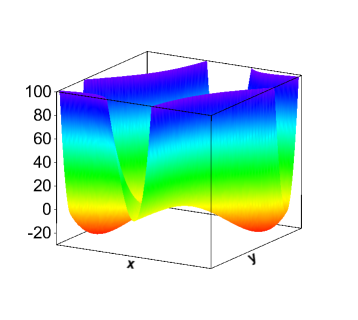
Figure 1: Landscape of $\phi(x,y)$ defined in Eq. (73), in the region satisfying $-5\leq x/d\leq 5$ and $-5\leq y/d\leq 5$, in the unit of $d^{4}$.

The next task is to find the minimum by a two-step procedure. First, $\phi(x,y)$ is minimized $\phi(x,y)$ with respect to $x$ for individual $y$, yielding a function $\phi_{c}(y)$,

$$\phi_{c}(y):=\min_{x}\phi(x,y)\,.$$ (77)

This minimization is accomplished via the first equation of Eq. (74),

$$\phi_{c}(y)=\min\big{[}\phi_{c0}(y),\phi_{c+}(y),\phi_{c-}(y)\big{]}=\left\{\begin{aligned} \phi_{c0}(y)&\quad(\mbox{for}~{}y\leq-3d~{}\mbox{and}~{}y\geq 3d)\\ \phi_{c+}(y)&\quad(\mbox{for}~{}0\leq y<3d)\\ \phi_{c-}(y)&\quad(\mbox{for}~{}-3d<y<0)\end{aligned}\right.\,,$$ (78)

where

$$\phi_{c0}(y)=\phi(0,y)=0\,,\quad\phi_{c\pm}(y)=\phi(y\pm d,y)=(y\pm d)^{3}(y\mp 3d)\,.$$ (79)

As shown in Fig. 2, $\phi_{c}(y)$ takes a minimum at $y=\pm 2d$, satisfying

$$\min_{y}\phi_{c}(y)=\min_{(x,y)}\phi(x,y)=-27d^{4}\,.$$ (80)

However, $\phi_{c}(y)$ is not differentiable at $y=0$ and $\pm 3d$, as seen in Fig. 2. Thus, the differentiability is lost in $\phi_{c}(y)$ at the global level, though it could hold within limited domains, e.g., $0<y<3d$. The violation of differentiability at the global level indicates the non-existence of universal function, as exemplified in Eq. (78). It is problematic to apply variational procedures without knowing the analyticity of $\phi_{c}(y)$, possibly hampering practicality.

Figure 2: $\phi_{c}(y)$ of Eq. (78) (solid line), and $\phi_{c0}(y),\phi_{c\pm}(y)$ of Eq. (79) (dashed lines).

Appendix C Energy density functional for 1-dimensional harmonic oscillator

While the original HK theorem assures the existence of an EDF in which the energy is represented as a functional only of the local density $n(\mathbf{r})$, modification via the KS theory has been needed in its practical application to many-fermion systems. This fact is linked to the shell structure that often emerges in many-fermion systems. To illustrate this situation and help to comprehend the path from the HK theorem to the KS theory, we consider a simple system under the 1-dimensional harmonic oscillator (h.o.) potential.

Let us take the Hamiltonian of the 1-dimensional h.o.,

$$H=K+U\,;\quad K=-\frac{1}{2m}\,\frac{d^{2}}{dx^{2}}\,,~{}U(x)=\frac{m\omega^{2}}{2}x^{2}\,.$$ (81)

This Hamiltonian gives energy levels $\epsilon_{\nu}=(\nu+\frac{1}{2})\omega$ $(\nu=0,1,2,\cdots)$, which can be regarded as orbits. We assume that each level has $\Omega$-fold degeneracy, and $N$ non-interacting fermions occupy the orbits. All particles occupy the $\nu=0$ orbit at the g.s. for $0<N\leq\Omega$, $(N-\Omega)$ particles occupy the $\nu=1$ orbit for $\Omega<N\leq 2\Omega$, and so forth, providing the g.s. energy and density,

$$\begin{split}&E^{(0)}_{N}=\left\{\begin{array}[]{ll}\frac{1}{2}N\omega&(0<N\leq\Omega)\\ \big{[}\frac{1}{2}\Omega+\frac{3}{2}(N-\Omega)\big{]}\omega&(\Omega<N\leq 2\Omega)\\ \quad\vdots&\end{array}\right.\,,\\ &\quad n^{(0)}_{N}(x)=\left\{\begin{array}[]{ll}{\displaystyle\sqrt{\frac{m\omega}{\pi}}\,N\,e^{-m\omega x^{2}}}&(0<N\leq\Omega)\\ {\displaystyle\sqrt{\frac{m\omega}{\pi}}\,\big{[}\Omega+2(N-\Omega)m\omega x^{2}\big{]}\,e^{-m\omega x^{2}}}&(\Omega<N\leq 2\Omega)\\ \quad\vdots&\end{array}\right.\,.\end{split}$$ (82)

This system is treated by the EDF under the HK theorem with $\mathbf{Q}=n(x)$.

The minimization of Eq. (16) can be substituted by the Legendre transformation around the minimum. The main task is constructing the kinetic part of the EDF. The kinetic part of the EDF is desirable not to depend on $U$, which is conjugate to $\mathbf{Q}\,(=n(x))$. For $0<N\leq\Omega$, the following EDF Stringari and Treiner (1987) is exact,

$$E^{\mathrm{HK}}[n]=\int dx\,\bigg{[}\frac{1}{8m}\,\frac{\big{(}n^{\prime}(x)\big{)}^{2}}{n(x)}+U(x)\,n(x)\bigg{]}\,.$$ (83)

Indeed, the variational equation of $E^{\mathrm{HK}}[n]$ with respect to $n(x)$ under the constraint $\int dx\,n(x)=N$,

$$\delta\tilde{E}^{\mathrm{HK}}[n]=0\,;\quad\tilde{E}^{\mathrm{HK}}[n]:=E^{\mathrm{HK}}[n]-\mu\bigg{[}\,\int dx\,n(x)-N\bigg{]}\,,$$ (84)

yields

$$\frac{1}{4m}\bigg{[}\frac{n^{\prime\prime}(x)}{n(x)}-\frac{1}{2}\Big{\{}\frac{n^{\prime}(x)}{n(x)}\Big{\}}^{2}\bigg{]}-U(x)+\mu=0\,,$$ (85)

coinciding with Eq. (82) when $U(x)=m\omega^{2}x^{2}/2$ and $\mu=\epsilon_{0}$.

The EDF of Eq. (83) is not appropriate as it is in $N>\Omega$. The exact energy and density of Eq. (82) for $\Omega<N\leq 2\Omega$ do not satisfy Eq. (84). On the other hand, it is always possible to obtain an exact functional around a fixed $N=N_{0}$ in terms of $\mathit{\Delta}n(x):=n(x)-n^{(0)}_{N_{0}}(x)$,

$$E^{\mathrm{HK}}[\mathit{\Delta}n]-E^{(0)}_{N_{0}}=\int dx\,\bigg{[}\frac{1}{8m}\,\frac{\big{(}\mathit{\Delta}n^{\prime}(x)\big{)}^{2}}{\mathit{\Delta}n(x)}+U(x)\,\mathit{\Delta}n(x)\bigg{]}\,,$$ (86)

because $\mathit{\Delta}n(x)\propto|\varphi_{\nu_{\mathrm{F}}}(x)|^{2}$ ($\nu_{\mathrm{F}}$ is the orbit just above $N_{0}$). However, Eq. (86) does not hold across $N=\Omega$; the EDF of (86) is not correct if $N_{0}<\Omega<N$. For Eq. (86) to be valid for $N>\Omega$, $n^{(0)}_{N_{0}}(x)$ and $E^{(0)}_{N_{0}}$ have to be redefined by shifting $N_{0}$. This result provides evidence that the EDF guaranteed by the HK theorem (Eq. (16)) is not regular everywhere. This irregularity comes out because of the shell structure, i.e., because the particles start occupying the $\nu=1$ orbit for $N>\Omega$. The source of the irregularity is the kinetic energy.

In contrast, the g.s. energy is immediately written with the 1-body density matrix in the present non-interacting problem. In the coordinate representation, the density matrix is $\varrho(x,x^{\prime}):=\langle\Psi|\psi^{\dagger}(x^{\prime})\,\psi(x)|\Psi\rangle$, where $\psi(x)$ and $\psi^{\dagger}(x)$ are field operators. The energy is exactly expressed as

$$E[\varrho]=\int dx\,dx^{\prime}\,\delta(x-x^{\prime})\bigg{[}\frac{1}{2m}\,\frac{\partial^{2}}{\partial x\,\partial x^{\prime}}\varrho(x,x^{\prime})+U(x)\,\varrho(x,x^{\prime})\bigg{]}\,.$$ (87)

Identifying the kinetic term as the irregular part and handling it as discussed in Sec. IV, the EDF reaches

$$\begin{split}E^{\mathrm{KS}}[\varrho;n]&=\frac{1}{2m}\int dx\,dx^{\prime}\,\delta(x-x^{\prime})\,\frac{\partial^{2}}{\partial x\,\partial x^{\prime}}\varrho(x,x^{\prime})+\int dx\,U(x)\,n(x)\\ &=-\frac{1}{2m}\int dx\,dx^{\prime}\,\delta^{\prime\prime}(x-x^{\prime})\,\varrho(x,x^{\prime})+\int dx\,U(x)\,n(x)\,,\end{split}$$ (88)

equivalent to Eq. (87). The EDF of (88) is global and differentiable with respect to $(\varrho,n)$.

References

• Parr and Yang (1989) R. G. Parr and W. Yang, Density-Functional Theory of Atoms and Molecules (Oxford Univ. Press, Oxford, 1989).
• Giuliani and Vignale (2005) G. F. Giuliani and G. Vignale, Quantum Theory of the Electron Liquid (Cambridge Univ. Press, Cambridge, 2005).
• Engel and Dreizler (2011) E. Engel and R. M. Dreizler, Density Functional Theory (Springer-Verlag, Berlin, 2011).
• Sahni (2016) V. Sahni, Quantal Density Functional Theory, 2nd ed. (Springer-Verlag, Berlin, 2016).
• Hohenberg and Kohn (1964) P. Hohenberg and W. Kohn, Phys. Rev. 136, B864 (1964).
• Kohn and Sham (1965) W. Kohn and L. J. Sham, Phys. Rev. 140, A1133 (1965).
• von Barth and Hedin (1972) U. von Barth and L. Hedin, J. Phys. C 5, 1629 (1972).
• Gunnarsson and Lundqvist (1976) O. Gunnarsson and B. I. Lundqvist, Phys. Rev. B 13, 4274 (1976).
• Jacob and Reiher (2012) C. R. Jacob and M. Reiher, Int. J. Quant. Chem. 112, 3661 (2012).
• Vignale and Rasolt (1987) G. Vignale and M. Rasolt, Phys. Rev. Lett. 59, 2360 (1987).
• Vignale and Rasolt (1988) G. Vignale and M. Rasolt, Phys. Rev. B 37, 10685 (1988).
• Oliveira et al. (1988) L. N. Oliveira, E. K. U. Gross,  and W. Kohn, Phys. Rev. Lett. 60, 2430 (1988).
• Lüders et al. (2005) M. Lüders, M. A. L. Marques, N. N. Lathiotakis, A. Floris, G. Profeta, L. Fast, A. Continenza, S. Massidda,  and E. K. U. Gross, Phys. Rev. B 72, 024545 (2005).
• Donnely and Parr (1978) R. A. Donnely and R. G. Parr, J. Chem. Phys. 69, 4431 (1978).
• Zumbach and Maschke (1985) G. Zumbach and K. Maschke, J. Chem. Phys. 82, 5604 (1985).
• Schindlmayr and Godby (1995) A. Schindlmayr and R. W. Godby, Phys. Rev. B 51, 10427 (1995).
• López-Sandoval and Pastor (2000) R. López-Sandoval and G. M. Pastor, Phys. Rev. B 61, 1764 (2000).
• Requistl and Pankratov (2008) R. Requistl and O. Pankratov, Phys. Rev. B 77, 235121 (2008).
• Pernal and Giesbertz (2016) K. Pernal and K. J. H. Giesbertz, Top. Curr. Chem. 368, 125 (2016).
• Higuchi and Higuchi (2004) M. Higuchi and K. Higuchi, Phys. Rev. B 69, 035113 (2004).
• Mermin (1965) N. D. Mermin, Phys. Rev. 137, A1441 (1965).
• Runge and Gross (1984) E. Runge and E. K. U. Gross, Phys. Rev. Lett. 52, 997 (1984).
• Gross and Kohn (1985) E. K. U. Gross and W. Kohn, Phys. Rev. Lett. 55, 2850 (1985).
• Vautherin and Brink (1972) D. Vautherin and D. M. Brink, Phys. Rev. C 5, 626 (1972).
• Skyrme (1959) T. H. R. Skyrme, Nucl. Phys. 9, 615 (1959).
• Petkov and Stoitsov (1991) I. Z. Petkov and M. V. Stoitsov, Nuclear Density Functional Theory (Oxford Univ. Press, Oxford, 1991).
• Colò (2020) G. Colò, Adv. Phys.: X 5, 1740061 (2020).
• Dechargé and Gogny (1980) J. Dechargé and D. Gogny, Phys. Rev. C 21, 1568 (1980).
• Nakada (2003) H. Nakada, Phys. Rev. C 68, 014316 (2003).
• Serot and Walecka (1986) B. D. Serot and J. D. Walecka, “The Relativistic Nuclear Many-Body Problem,” in Advances in Nuclear Physics, Vol. 16, edited by J. W. Negele and E. Vogt (Plenum, New York, 1986) pp. 1–320.
• Ring (2016) P. Ring, “Concept of covariant density functional theory,” in International Review of Nuclear Physics, Vol. 10, edited by J. Meng (World Scientific, Singapore, 2016) pp. 1–20.
• Thomas (1927) L. H. Thomas, Math. Proc. Camb. Phil. Soc. 23, 542 (1927).
• Fermi (1928) E. Fermi, Z. Phys. 48, 73 (1928).
• Deb and Chattaraj (1988) B. M. Deb and P. K. Chattaraj, Phys. Rev. A 37, 4030 (1988).
• Deb and Chattaraj (1992) B. M. Deb and P. K. Chattaraj, Phys. Rev. A 45, 1412 (1992).
• Pearson et al. (1993) M. Pearson, E. Smargiassi,  and P. A. Madden, J. Phys.: Cond. Matt. 5, 3221 (1993).
• Ring and Schuck (1980) P. Ring and P. Schuck, The Nuclear Many-Body Problem (Springer-Verlag, New York, 1980).
• Reichl (1980) L. E. Reichl, A Modern Course in Statistical Physics (Univ. Texas Press, Austin, 1980).
• Lieb (1981) E. H. Lieb, Phys. Rev. Lett. 46, 457 (1981).
• Gilbert (1975) T. L. Gilbert, Phys. Rev. B 12, 2111 (1975).
• Fukuda et al. (1994) R. Fukuda, T. Kotani, Y. Suzuki,  and S. Yokojima, Prog. Theor. Phys. 92, 833 (1994).
• Valiev and Fernando (1997) M. Valiev and G. W. Fernando,   (1997), arXiv:cond-mat.str-el/9702247 [cond-mat.str-el] .
• Levy (1979) M. Levy, Proc. Natl. Acad. Sci. USA 76, 6062 (1979).
• Coleman (1963) A. J. Coleman, Rev. Mod. Phys. 35, 668 (1963).
• Harriman (1981) J. E. Harriman, Phys. Rev. A 24, 680 (1981).
• Levy (1982) M. Levy, Phys. Rev. A 26, 1200 (1982).
• Capelle and Vignale (2001) K. Capelle and G. Vignale, Phys. Rev. Lett. 86, 5546 (2001).
• Kvaal et al. (2014) S. Kvaal, U. Ekström, A. M. Teale,  and T. Helgaker, J. Chem. Phys. 140, 18A518 (2014).
• Valone (1980) A. M. Valone, J. Chem. Phys. 73, 1344 (1980).
• Messiah (1961) A. Messiah, Quantum Mechanics, vol. 2 (Elsevier, Amsterdam, 1961).
• Sahni et al. (1988) V. Sahni, K.-P. Bohnen,  and M. K. Harbola, Phys. Rev. A 37, 1895 (1988).
• Perdew et al. (1996) J. P. Perdew, K. Burke,  and M. Ernzerhof, Phys. Rev. Lett. 77, 3865 (1996).
• Tao et al. (2003) J. Tao, J. P. Perdew, V. N. Staroverov,  and G. E. Scuseria, Phys. Rev. Lett. 91, 146401 (2003).
• Nagai et al. (2022) R. Nagai, R. Akashi,  and O. Sugino, Phys. Rev. Res. 4, 013106 (2022).
• Drut et al. (2010) J. E. Drut, R. J. Furnstahl,  and L. Platter, Prog. Part. Nucl. Phys. 64, 120 (2010).
• Engel (2007) J. Engel, Phys. Rev. C 75, 014306 (2007).
• Nakada (2020) H. Nakada, Int. J. Mod. Phys. E 29, 1930008 (2020).
• Barnea (2007) N. Barnea, Phys. Rev. C 76, 067302 (2007).
• Messud et al. (2009) J. Messud, M. Bender,  and E. Suraud, Phys. Rev. C 80, 054314 (2009).
• Messud (2013) J. Messud, Phys. Rev. C 87, 024302 (2013).
• Negele and Vautherin (1972) J. W. Negele and D. Vautherin, Phys. Rev. C 5, 1472 (1972).
• Campi and Sprung (1972) X. Campi and D. W. Sprung, Nucl. Phys. A 194, 401 (1972).
• Kortelainen et al. (2012) M. Kortelainen, J. McDonnell, W. Nazarewicz, P.-G. Reinhard, J. Sarich, N. Schunck, M. V. Stoitsov,  and S. M. Wild, Phys. Rev. C 85, 024304 (2012).
• Kortelainen et al. (2014) M. Kortelainen, J. McDonnell, W. Nazarewicz, E. Olsen, P.-G. Reinhard, J. Sarich, N. Schunck, S. M. Wild, D. Davesne, et al., Phys. Rev. C 89, 054314 (2014).
• Mahaux et al. (1985) C. Mahaux, P. F. Bortignon, R. A. Broglia,  and C. H. Dasso, Phys. Rep. 120, 1 (1985).
• Kaiser et al. (2003) N. Kaiser, S. Fritsch,  and W. Weise, Nucl. Phys. A 724, 47 (2003).
• Navarro Pérez et al. (2018) R. Navarro Pérez, N. Schunck, A. Dyhdalo, R. J. Furnstahl,  and S. K. Bogner, Phys. Rev. C 97, 054304 (2018).
• Shen et al. (2019) S. Shen, H. Liang, W. H. Long, J. Meng,  and P. Ring, Prog. Part. Nucl. Phys. 109, 103713 (2019).
• Baldo et al. (2008) M. Baldo, P. Schuck,  and X. Viñas, Phys. Lett. B 663, 390 (2008).
• Bohr and Mottelson (1975) A. Bohr and B. R. Mottelson, Nuclear Structure, vol. 2 (Benjamin, Reading, 1975).
• Giraud et al. (2008) B. G. Giraud, B. K. Jennings,  and B. R. Barrett, Phys. Rev. A 78, 032507 (2008).
• Nakada (2016) H. Nakada, Prog. Theor. Exp. Phys. 2016, 063D02 (2016).
• Stringari and Treiner (1987) S. Stringari and J. Treiner, Phys. Rev. B 36, 8369 (1987).