LISA Sensitivity and SNR Calculations

N/Ref :	LISA-LCST-SGS-TN-001
Title	LISA Sensitivity and SNR Calculations
Abstract	This Technical Note (LISA reference LISA-LCST-SGS-TN-001) describes the computation of the noise power spectral density, the sensitivity curve and the signal-to-noise ratio for LISA (Laser Interferometer Antenna). It is an applicable document for ESA (European Space Agency) and the reference for the LISA Science Requirement Document.

	Name	Date
Prepared by	S. Babak (APC), M. Hewitson (AEI) and A. Petiteau1 (APC)
Checked by	LISA Science Study Team	2021/06/30
Approved by	LISA Science Study Team	2021/06/30

¹ contact: petiteau@apc.in2p3.fr

Contributor List

Author’s name	Institute	Location
Babak Stas	APC	Paris-France
Petiteau Antoine	APC	Paris-France
Hewitson Martin	AEI	Hannover-Germany

Document Change Record

Ver.	Date	Author	Description	Pages
0.0	2018/05/22	S. Babak (APC), M. Hewitson(AEI), A. Petiteau (APC)	First Version	all
0.1	2018/05/22	M. Hewitson (AEI)	Criculate in SST + reviewers for comments	all
0.2	2018/08/13	A. Petiteau (APC)	Implementing comments/corrections from D. Shoemaker, P. Jetzer and M. Colpi	all
0.3	…	S. Babak (APC)	Some small corrections and comments implemented	all
0.4	2020/01/08	A. Petiteau (APC)	Update all results using new LDC convetions; update TDI part	all
0.6	2020/05/20	A. Petiteau (APC), S. Babak (APC), M. Hewitson (AEI)	Add executive summary, more justification on sensitivity	all
0.7	2020/07/06	S. Babak (APC)	Reorganisation	all
0.8	2021/01/19	A. Petiteau (APC)	Consolidation, Change of conventions	all
0.9	25/02/2021	S. Babak (APC)	Rewriting semi-analytic response, adjusting Galactic foreground	all
0.10	19/03/2021	A. Petiteau (APC)	Rewriting semi-analytic response, adjusting Galactic foreground	all
0.11	19/03/2021	A. Petiteau (APC)	Add small annexe deriving noise PSD from SciRD sensitivity	appendix B
0.12	23/05/2021	A. Petiteau (APC)	Fix after review from SST	all
1.0	31/07/2021	A. Petiteau (APC)	First official release	all

Distribution list

Recipient	Restricted	Not restricted
LISA Consortium		✗

1 Executive Summary

This note describes the calculations made to compute science performance for Laser Interferometer Space Antenna (LISA) , in particular it presents a sensitivity curve that is in-line with the formula given in the Science Requirement Document (SciRD),[12].

The formula for the required strain sensitivity curve is given in a way that is implementation agnostic, i.e., it doesn’t assume a particular observatory configuration (interferometery, arm-length, number of links, etc). An appropriate sky-averaged formulation of a sensitivity curve for the current set of observatory parameters (6 interferometric links, each 2.5 Gm long) is given in Section 6, and is shown graphically compared to the SciRD in Figure 1. This model assumes an interferometer noise of 15 pm$/\sqrt{\rm Hz}$ and a test-mass acceleration noise of 3 $\textrm{fm}/\textrm{s}^{2}/\sqrt{\rm Hz}$ with the noise-shape functions as described in that section.

Note: the slight differences between the sensitivity model and the formulaic curve from the SciRD arise from the difference in the arm-response models.

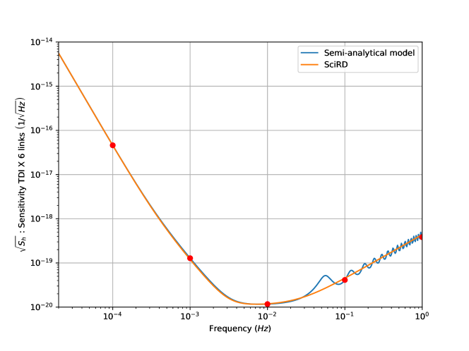
Figure 1: A comparison of the SciRD [12] sensitivity formula (see appendix B) to the sensitivity model given in section 6 for the 6-links configuration, i.e. X,Y and Z TDI. The plot also includes the points tabulated in Table 3.

Most of the time we work in the geometrical units $G=c=1$, however we restore $G$, $c$ when their presence is not obvious.

All computations and figures can be reproduced from the associated notebook available at
https://gitlab.in2p3.fr/LISA/lisa_sensitivity_snr/ [1].

2 Define the sensitivity

The definition of the sensitivity is closely related to the signal-to-noise ratio Signal-to-Noise Ratio (SNR) which for the deterministic source we define as

$$SNR^{2}=4\operatorname{Re}\left(\int_{0}^{f_{\textrm{max}}}df\frac{\tilde{X}\tilde{X}^{*}}{S_{n}(f)}\right),$$ (1)

where we have introduced the one-sided noise power spectral density $S_{n}(f)$ and the signal $\tilde{X}(f)$ (in Fourier domain) as it appears at the detector’s output plus post-processing (TDI for example). The noise Power Spectral Density (PSD) is defined as

$$E[\tilde{n}(f)\tilde{n}(f^{\prime})]=\frac{1}{2}\delta(f-f^{\prime})S_{n}(f)$$ (2)

where $E[...]$ is the expectation value, $\tilde{n}(f)$ is the noise in Fourier domain and $\delta$ is the Dirac delta distribution. For completeness we’ll write it in the time domain as well:

$$E[n(t)n(t^{\prime})]=\int_{-\infty}^{+\infty}df\ S_{n}(|f|)e^{-i2\pi f(t-t^{\prime})}.$$ (3)

The measurement $\tilde{X}(f)$ (signal) contains the detector’s response and traces of any data post-processing (filters, TDI, …), we can write it as:

$$\tilde{X}(f)=R_{+}(f,t,\theta_{s},\phi_{s},\psi)\tilde{h}_{+}(f)+R_{\times}(f,t,\theta_{s},\phi_{s},\psi)\tilde{h}_{\times}(f)$$ (4)

where $h_{+,\times}$ is a GW signal in the source/radiation frame and $R_{+,\times}$ is the detector’s (LISA) response to each polarization which depends on the sky location of the source $\theta_{s},\phi_{s}$ and on polarization angle $\psi$. In general, response is a function of instantaneous frequency and the corresponding time (defining LISA’s position on the orbit). We define the sensitivity using the ${\rm SNR}^{2}$ averaged over the sky and polarization:

$$<SNR^{2}>=4\operatorname{Re}\left(\int_{0}^{f_{\rm max}}df\frac{\tilde{h}_{+}^{2}+\tilde{h}^{2}_{\times}}{S_{n}(f)/<|R_{L}|^{2}>}\right)$$ (5)

where $<...>$ we use for the polarization and sky averaging:

$$<...>=\frac{1}{2\pi}\int_{0}^{2\pi}d\psi\frac{1}{4\pi}\int d^{2}\Omega...$$ (6)

and we have introduced $<|R_{L}|^{2}>=<|R_{+}|^{2}>=<|R_{\times}|^{2}>$ (see section 5.2 for detailed on the averaged antenna response functions). We define the sensitivity as

$$S_{h}(f)=\frac{S_{n}(f)}{<|R_{L}|^{2}>}$$ (7)

this definition could be extended to the isotropic stochastic signal with PSD in each polarization $P_{+},\;P_{\times}$:

$$SNR^{2}=T\int\,df\frac{P_{+}(f)+P_{\times}(f)}{S_{n}(f)/<|R_{L}|^{2}>}$$ (8)

3 Instrumental noise

The computation of the sensitivity curve presented above (see figure 1) is detailed in section 6.1. It should be essentially what we have in the SciRD [12], though the high-frequency wiggles are deliberately taken out in the SciRD. It corresponds to a simplified observatory with a noise described by only two components (see appendix B for correspondance between sensitivity and noise PSD).

The first one is the high frequency noise component, given as a displacement noise of $15\text{\,}\mathrm{pm}\text{/}\mathrm{\sqrt{\text{}}}$ rising with $f^{2}$, and described as

$$\sqrt{S_{OMS}}(f) = 15\,\left[\frac{\textrm{pm}}{\sqrt{\textrm{Hz}}}\right]\sqrt{1+\left(\frac{2\times 10^{-3}}{f}\right)^{4}},$$ (9)

$$\sqrt{S^{OMS}_{d\nu/\nu}}(f) = 15\times 10^{-12}\,\frac{2\pi f}{c}\left[\frac{1}{\sqrt{\textrm{Hz}}}\right]\sqrt{1+\left(\frac{2\times 10^{-3}}{f}\right)^{4}}$$ (10)

The second one is the low frequency noise component, given as an acceleration noise of 3 $\mathrm{f}\mathrm{m}\,\mathrm{s}^{-2}\mathrm{/}\mathrm{\sqrt{\text{}}}$, rising with $f^{2}$ below $0.4\text{\,}\mathrm{mHz}$, and described as

$$\sqrt{S_{acc}}(f) = 3\,\left[\frac{\textrm{fm}.\textrm{s}^{-2}}{\sqrt{\textrm{Hz}}}\right]\sqrt{1+\left(\frac{0.4\times 10^{-3}}{f}\right)^{2}}\sqrt{1+\left(\frac{f}{8\times 10^{-3}}\right)^{4}}$$ (11)

$$\sqrt{S^{acc}_{dL}}(f) = {3\over\left(2\pi f\right)^{2}}\,\left[\frac{\textrm{fm}}{\sqrt{\textrm{Hz}}}\right]\sqrt{1+\left(\frac{0.4\times 10^{-3}}{f}\right)^{2}}\sqrt{1+\left(\frac{f}{8\times 10^{-3}}\right)^{4}},$$ (12)

$$\sqrt{S^{acc}_{d\nu/\nu}}(f) = {3\times 10^{-15}\over 2\pi fc}\,\left[\frac{1}{\sqrt{\textrm{Hz}}}\right]\sqrt{1+\left(\frac{0.4\times 10^{-3}}{f}\right)^{2}}\sqrt{1+\left(\frac{f}{8\times 10^{-3}}\right)^{4}}.$$ (13)

The formulation (11) is in unit of acceleration, (9) and (12) in unit of displacement and (10) and (13) in unit of relative frequency.

3.1 Noise PSD

In the following we are describing the analytic model of the one-sided noise PSD, $S_{n}(f)$, and how it is derived from the noise components in each interferometric measurements. We will explicitly show $S_{n}(f)$ for a Michelson-type TDI generator. The one-sided noise PSD is used in the matched filtering and, as a result, enters the likelihood function and SNR.

Figure 2: Schematic representation of the LISA constellation. The bullet points inside of each spacecraft denote the test masses (TMs). The spacecrafts are numbered and the direction of propagation of the laser light is explicitly labeled as subscripts. We do not detail the connection between TMs inside the s/c.

We refer to Fig. 2 for labeling of the spacecrafts (s/c) and test masses ( test mass, often proof mass (TM)). We just consider the top-level noise sources here, i.e. the two components described above, namely $S_{acc_{ij}}$ representing the low-frequency noise on the Moving Optical Sub-Assembly (MOSA) of spacecraft $i$ and facing spacecraft $j$ and $S_{OMS_{ij}}$ describing the high-frequency noise of the same MOSA. We refer to the Performance TN [11] for more details on the noise budget.

The reference measurement is the TDI generator X given, for generation 1.5 and 2.0, by:

$$X_{1.5} = \eta_{13}+D_{13}\eta_{31}+D_{13}D_{31}\eta_{12}+D_{13}D_{31}D_{12}\eta_{21}-\eta_{12}-D_{12}\eta_{21}-D_{12}D_{21}\eta_{13}-D_{12}D_{21}D_{13}\eta_{31}$$ (14)

$$X_{2.0} = \eta_{13}+D_{13}\eta_{31}+D_{13}D_{31}\eta_{12}+D_{13}D_{31}D_{12}\eta_{21}+D_{13}D_{31}D_{12}D_{21}\eta_{12}$$ (16)

$$+D_{13}D_{31}D_{12}D_{21}D_{12}\eta_{21}+D_{13}D_{31}D_{12}D_{21}D_{12}D_{21}\eta_{13}+D_{13}D_{31}D_{12}D_{21}D_{12}D_{21}D_{13}\eta_{31}$$

$$-\eta_{12}-D_{12}\eta_{21}-D_{12}D_{21}\eta_{13}-D_{12}D_{21}D_{13}\eta_{31}-D_{12}D_{21}D_{13}D_{31}\eta_{13}$$

$$-D_{12}D_{21}D_{13}D_{31}D_{13}\eta_{31}-D_{12}D_{21}D_{13}D_{31}D_{13}D_{31}\eta_{12}-D_{12}D_{21}D_{13}D_{31}D_{13}D_{31}D_{12}\eta_{21}$$

with $\eta_{ij}$ the cleaned science measurement MOSA on spacecraft $i$ and receiving the signal from the s/c $j$ and $D_{ij}x(t)=x(t-L_{ij}/c)$ the delay operator along the link from s/c $j$ to s/c $i$.

Here we give the final expression for the noise PSD with different level of approximation. The detailed derivation is given in the Appendix A.

Approximation TDI-1.: Armlength are constant, i.e. the delay operators are commuting and we can use TDI generation 1.5,

$$S_{n,X_{1.5}}=PSD_{X_{1.5}}=4\sin^{2}\left(\omega{L_{31}+L_{13}\over 2}\right)\left(S_{OMS_{12}}+S_{OMS_{21}}+4S_{acc_{21}}+4\cos^{2}\left(\omega{L_{12}+L_{21}\over 2}\right)S_{acc_{12}}\right)$$

$$+4\sin^{2}\left(\omega{L_{21}+L_{12}\over 2}\right)\left(S_{OMS_{13}}+S_{OMS_{31}}+4S_{acc_{31}}+4\cos^{2}\left(\omega{L_{31}+L_{13}\over 2}\right)S_{acc_{13}}\right)$$ (17)

Approximation TDI-2.: All armlength equal : $L_{ij}=L$. With this approximation, the PSD is:

$$S_{n,X_{1.5}}=PSD_{X_{1.5}}=4\sin^{2}\left(\omega L\right)\left(S_{OMS_{12}}+S_{OMS_{21}}+S_{OMS_{13}}+S_{OMS_{31}}+4\left(S_{acc_{21}}+S_{acc_{31}}+\cos^{2}\left(\omega L\right)\left(S_{acc_{12}}+S_{acc_{13}}\right)\right)\right)$$

(18)

Approximation TDI-3.: All noises of the same type have the same PSD : $S_{OMS_{ij}}=S_{OMS}$ and $S_{acc_{ij}}=S_{acc}$ With this approximation, the PSD is:

$$S_{n,X_{1.5}}=PSD_{X_{1.5}}=16\sin^{2}\left(\omega L\right)\left(S_{OMS}+\left(3+\cos\left(2\omega L\right)\right)S_{acc}\right)$$ (19)

The figure 3 shows the comparison for TDI 1.5 between numerical simulation by the simulator LISACode [15, 14] and the analytical formulation (19).

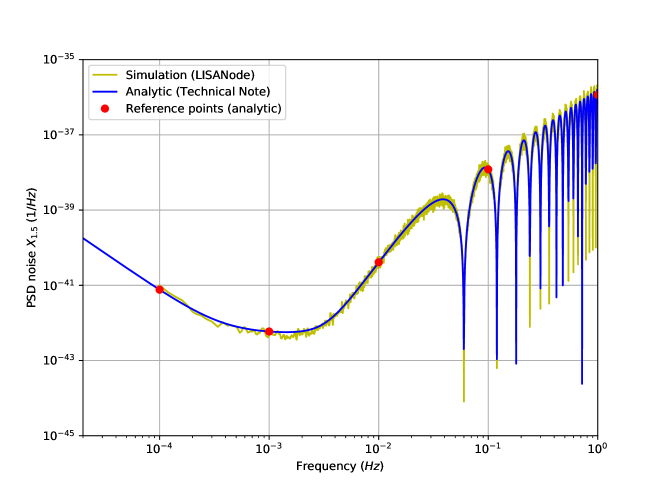
Figure 3: Noise of TDI $X_{1.5}$: comparison between numerical simulation with the simulator LISANode [5, 4] (version 1.2; varying armlength according to the keplerian orbit), LDC and analytical formulation (19). The plot also includes the points tabulated in Table 1. The discrepancy of the simulation at high frequency is due to the low sampling rate and simplified anti-aliasing filtering used for this particular simulation.

In reality, in order to suppress the laser noise we need to consider the flexing of the arms, and, therefore, use TDI $X_{2.0}$:

$$S_{n,X_{2.0}}=PSD_{X_{2.0}}=64\sin^{2}\left(\omega L\right)\sin^{2}\left(2\omega L\right)\left(S_{OMS}+\left(3+\cos\left(2\omega L\right)\right)S_{acc}\right)$$ (20)

The figure 4 shows the comparison for TDI 2.0 between numerical simulation by LISANode [5, 4] and the analytical formulation (20).

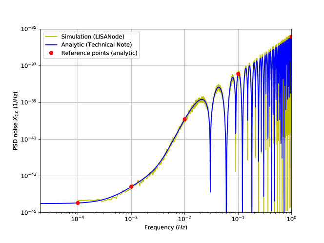
Figure 4: Noise of TDI $X_{2.0}$: comparison between numerical simulation with LISANode, LDC and analytical formulation (20). The plot also includes the points tabulated in Table 1.

The table 1 is providing the value for the reference frequency points.

Frequency (Hz)	$PSD_{X_{1.5},\rm SciRD}$	$PSD_{X_{2.0},\rm SciRD}$
0.00010	7.645865e-42	3.358340e-45
0.00100	5.901951e-43	2.580670e-44
0.01000	4.099978e-41	1.227169e-40
0.10000	1.206944e-38	3.628698e-38
1.00000	1.152922e-36	3.737383e-36

Table 1: The numerical values of the PSD of noises in TDI $X_{1.5}$ and $X_{2.0}$ for some fixed frequencies. For reference we also give the PSD for the curve given in the SciRD [12].

4 GW response for X-Michelson TDI

Here we will introduce the notation for GW signal as it is seen at the output of applying TDI procedure. Most of our notations are presented schematically in Fig. 2, note that for the GW response we will always assume that $L_{sr}=L_{rs}=L$. The single link response (the laser light emitted by “s”ender to the “r”eceiver, traveling along link “rs”) to GW is given in relative frequency as

$$y_{rs}^{GW}=\frac{\Phi_{rs}(t_{s}-\hat{k}.\vec{R}_{s}(t_{s}))-\Phi_{rs}(t-\hat{k}.\vec{R}_{r}(t))}{2(1-\hat{k}.\hat{n}_{rs})}$$ (21)

where $\hat{k}$ is direction of GW propagation, $\vec{R}_{s,r}$ vector position of a sender/receiver, $\hat{n}_{rs}$ a unit vector connecting sender and receiver (link). We have used the following notations

$$\Phi_{rs}=\hat{n}_{rs}h_{ij}\hat{n}_{rs}$$ (22)

which is projection of the GW strain on the link, $t_{s}=t-|\vec{R}_{r}(t)-\vec{R}_{s}(t_{s})|\approx t-L_{rs}$, and $L\hat{n}_{rs}\approx\vec{R}_{r}(t)-\vec{R}_{s}(t_{s})$, using this approximation we have

$$y_{rs}^{GW}=\frac{\Phi_{rs}(t-\hat{k}.\vec{R}_{s}-L_{rs})-\Phi_{rs}(t-\hat{k}.\vec{R}_{r})}{2(1-\hat{k}.\hat{n}_{rs})}$$ (23)

Substitute $h_{ij}$ decomposed in the polarization basis in the Solar System barycenter (SSB) we get

$$\Phi_{rs}=\hat{n}_{rs}\hat{n}_{rs}\left[h^{SSB}_{+}(\hat{u}\otimes\hat{u}-\hat{v}\otimes\hat{v})+h^{SSB}_{\times}(\hat{u}\otimes\hat{v}+\hat{v}\otimes\hat{u})\right]$$ (24)

The polarization basis is chosen as

$$\hat{u} = -\hat{e}_{\phi}\propto\left(\frac{\partial\hat{k}}{\partial\lambda}\right)=\{\sin{\lambda},\cos{\lambda},0\}$$ (25)

$$\hat{v} = -\hat{e}_{\theta}\propto\left(\frac{\partial\hat{k}}{\partial\beta}\right)=\{-\sin{\beta}\cos{\lambda},-\sin{\beta}\sin{\lambda},\cos{\beta}\}$$ (26)

where $\beta$ is ecliptic latitude and $\lambda$ ecliptic longitude of the source.

$$\hat{k}=-\hat{e}_{r}=-\{\cos{\beta}\cos{\lambda},\cos{\beta}\sin{\lambda},\sin{\beta}\}.$$ (27)

The polarizations in the SSB are related to the strain in the source (radiation frame) via polarization angle $\psi$:

$$h_{ij}^{SSB} = (h_{+}\cos{2\psi}-h_{\times}\sin{2\psi})\epsilon^{+}_{ij}+(h_{+}\sin{2\psi}+h_{\times}\cos{2\psi})\epsilon^{+}_{ij}$$ (28)

$$\epsilon^{+}_{ij} = (\hat{u}\otimes\hat{u}-\hat{v}\otimes\hat{v})_{ij}$$ (29)

$$\epsilon^{\times}_{ij} = (\hat{u}\otimes\hat{v}+\hat{v}\otimes\hat{u})_{ij}$$ (30)

Finally, to get the Gravitational Wave (GW) response to TDI X for greneration 1.5 and generation 2.0, we use the eqns (14) and (16) respectively without the noise in the measurement, i.e. $\eta_{ij}=y_{ij}$. We assume that the GW signal in the source frame can be presented as

$$h_{+}=A_{+}e^{i\Phi(t)},\;\;\;\;h_{\times}=-iA_{\times}e^{i\Phi(t)}$$ (31)

assuming that we add complex conjugate to make it real. Then we can write

$$X^{GW}_{1.5} = (\omega L)\sin{(\omega L)}e^{-i[\Phi(t-\hat{k}\vec{R}_{1})-\omega L]}\{A_{+}[F_{13}^{+}\Upsilon_{13}-F_{12}^{+}\Upsilon_{12}]+A_{\times}[F_{13}^{\times}\Upsilon_{13}-F_{12}^{\times}\Upsilon_{12}]\}$$ (32)

$$X^{GW}_{2.0} = 2i\sin{(2\omega L)}e^{-2i\omega L}X^{GW}_{1.5}.\$$ (33)

We have used the following notations:

$$F_{rs}^{+}=\hat{n}_{rs}^{i}\hat{n}_{rs}^{j}\left[\epsilon^{+}_{ij}\cos{2\psi}+\epsilon^{\times}_{ij}\sin{2\psi}\right],\,\,F_{rs}^{\times}=\hat{n}_{rs}^{i}\hat{n}_{rs}^{j}\left[-\epsilon^{+}_{ij}\sin{2\psi}+\epsilon^{\times}_{ij}\cos{2\psi}\right]$$ (34)

$$\Upsilon_{rs}=Sinc\left[\frac{\omega L}{2}(1-\hat{k}.\hat{n}_{rs})\right]e^{-i\frac{\omega L}{2}(1-\hat{k}.\hat{n}_{rs})}+Sinc\left[\frac{\omega L}{2}(1-\hat{k}.\hat{n}_{sr})\right]e^{-i\frac{\omega L}{2}(3+\hat{k}.\hat{n}_{sr})}$$ (35)

This form is convenient when computing the average response as we show in the next section.

5 Average GW response

By convention the sensitivity of a GW instrument is computed with the response averaged over source polarization and sky position. It is a useful form for calculating the observational capability. It can be computed using numerical simulation or semi-analytical formulation.

5.1 Using numerical simulations

The easiest way to numerically compute the response of the instrument averaged over polarization and sky is to use (8). We generate the point-like independent noise sources uniformly distributed on the sky and we randomly assign polarization angle to each source. If we use the noise level for each polarization component $1/2$, then the average PSD of a generate signal

$$<\rm{P_{GW}}>=<|R_{L}|>(P_{+}(f)+P_{\times}(f))=<|R_{L}|>$$

so we directly obtain the average response which can be used in computing the sensitivity. The advantage of using the white noise is that we cover all frequencies at once. . The alternative derivation based on the monochromatic sources will be presented in the next section. The simulated PSD for each source is shown in figure 5. We are numericlally averaging over polarization angle (performing monte carlo simulation) and we are simulating LISA observation (TDI computation) using LISACode and 192 white noise sources uniformly distributed over the sky . The PSD of each source requested by the simulator is $PSD_{src}=\frac{PSD_{total}}{2N_{src}}$.

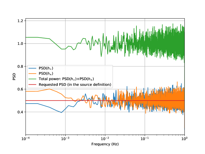
Figure 5: PSDs of simulation for one SGWB source with LISACode and configured as a white noise with at PSD=0.5 .

The figure 6 shows the numerical response for TDI $X_{1.5}$ according to the procedure described above.

5.2 Semi-analytical computation

A semi-analytical treatment for computing the average response to GW is described in [10].

We can reproduce it using the eqns. (32), (33) and using the definition (7). In other words we need to compute $<|X_{1.5}^{GW}|^{2}>$ . The averaging over polarization and sky position can be done analytically for the long-wavelength approximation and will be discussed in section 6.3. We introduce yet another notation:

$$F^{+}_{X}\equiv\frac{1}{4}\left[F_{13}^{+}\Upsilon_{13}-F_{12}^{+}\Upsilon_{12}\right],\;\;F^{\times}_{X}\equiv\frac{1}{4}\left[F_{13}^{\times}\Upsilon_{13}-F_{12}^{\times}\Upsilon_{12}\right]$$ (36)

in order to get the compact form:

$$<|X_{1.5}^{GW}|^{2}>=(4\omega L)^{2}\sin^{2}{(\omega L)}\left[A_{+}^{2}<(F^{+}_{X})^{2}>+A_{\times}^{2}<(F^{\times}_{X})^{2}>+2A_{+}A_{\times}<F^{+}_{X}F^{\times*}_{X}+F^{+*}_{X}F^{\times}_{X}>\right]$$ (37)

and note that $F^{+,\times}_{X}=F^{+,\times}_{X}(\psi,\hat{k};t)$. Unfortunately we have to perform averaging numerically. It can be shown (i.e. [10]) that the averaged antenna response functions $<(F^{+,\times}_{X})^{2}>$ do not depend on time, moreover $<(F^{+}_{X})^{2}>=<(F^{\times}_{X})^{2}>$, and the cross-term averages to zero $<F^{+}_{X}F^{\times*}_{X}+F^{+*}_{X}F^{\times}_{X}>=0$. This implies:

$$<|X_{1.5}^{GW}|^{2}>=(4\omega L)^{2}\sin^{2}{(\omega L)}<(F^{+}_{X})^{2}>[A_{+}^{2}+A_{\times}^{2}].$$ (38)

Using definition  (7) we get for the response ($X_{1.5}$) function to GW:

$$<R_{L,X_{1.5}}(f)>=(4\omega L)^{2}\sin^{2}{(\omega L)}<(F^{+}_{X})^{2}>.$$ (39)

Using the relation between 1.5 and 2.0 generation of TDI, given by eqn. (33) we get the average response $X_{2.0}$ to GW:

$$<R_{L,X_{2.0}}(f)>=(4\omega L)^{2}\sin^{2}{(\omega L)}(2\sin{(2\omega L)})^{2}<(F^{+}_{X})^{2}>.$$ (40)

The figure 6 shows the comparison between numerical response obtained for TDI $X_{1.5}$ and the semi-analytic treatment. Reference points are given in the Table 2.

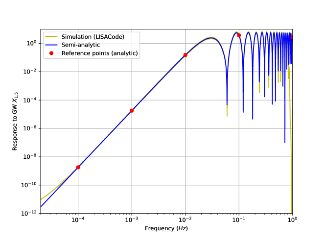
Figure 6: The numerical values of the response to GW for TDI $X_{1.5}$ for some fixed frequencies. The yellow curve corresponds to the reference numerical result (valid for $0.2mHz<f<0.5Hz$) and the blue to the analytical version from equation (39). The plot also includes in red the points tabulated in Table 2.

Frequency (Hz)	Analytic approx. $X_{1.5}$	$R_{\rm LISACode,X_{1.5}}$	Analytic approx. $X_{2.0}$	$R_{\rm LISACode,X_{2.0}}$
0.00010	1.808897e-09	1.906063e-09	7.945155e-13	7.372150e-12
0.00100	1.805606e-05	1.750219e-05	7.902030e-07	8.349357e-07
0.01000	1.503154e-01	1.593552e-01	4.513257e-01	4.427565e-01
0.10000	3.726972e+00	3.825690e+00	1.127471e+01	1.104438e+01
1.00000	2.836169e+00	-	6.804830e+00	-

Table 2: The numerical values of the response of TDI $X_{1.5}$ to GW for some fixed frequencies.

The comparison between the numerical and the semi-analytic response for TDI $X_{2.0}$ and the simulated data are shown on figure 7. Reference points are given in the Table 2

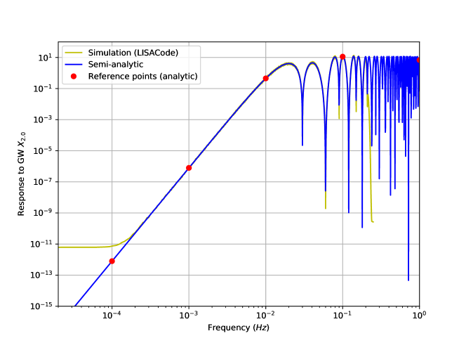
Figure 7: The numerical values of the response to GW for TDI $X_{2.0}$ for some fixed frequencies. The yellow curve corresponds to the reference numerical result (valid for $0.2mHz<f<0.1Hz$) and the blue to the analytical version from equation (40). The plot also includes in red the points tabulated in Table 2.

6 Sensitivity

6.1 Definition and reference

The sensitivity is obtained using the averaged response for $X$ described in section 5. It is defined as (similar to (7)):

$$S_{h,X}=\frac{PSD_{X}}{<|R_{L,X}|^{2}>}$$ (41)

We can also substitute explicitly the PSD and the averaged response function from previous subsections (formulas (39), (19),(40), (20)):

$$S_{h,X}=\frac{S_{OMS}+\left(3+\cos\left(2\omega L\right)\right)S_{acc}}{\left({\omega L}\right)^{2}\ <(F^{+}_{X})^{2}>}$$ (42)

NOTE: The expression of the sensitivity is the same for $X_{1.5}$ and for $X_{2.0}$ since the ratio of noise PSD and response to GW are identical, i.e (19) over (39) is equivalent to (20) over (40).

We on purpose kept the subscript $X$ to emphasize that this is a sensitivity for 4-links measurement which consists of only one Michelson TDI combination. For the 6 links (current LISA configuration), we can form 3 Michelson TDI combinations ($X,Y,Z$) which are not independent as they share one arm. We can form another TDI combination (referred as $A,E,T$) [17] which have (under simplified assumptions adopted here) independent noise and roughly maximise to “$+$”, “$\times$” polarizations and “null” stream (free of GW signal). This interpretation is especially good for long-wavelength approximation $\omega L\ll 1$. At high frequencies all three TDI combinations have a similar response to a GW signal. The key point is that if we use combined SNR to define the sensitivity then

$$S_{h}=S_{h,X}/2.$$ (43)

The strain sensitivity to only $X$, $\sqrt{S_{h,X}}$, is plotted in fig. 8 and some points are tabulated in table 3.

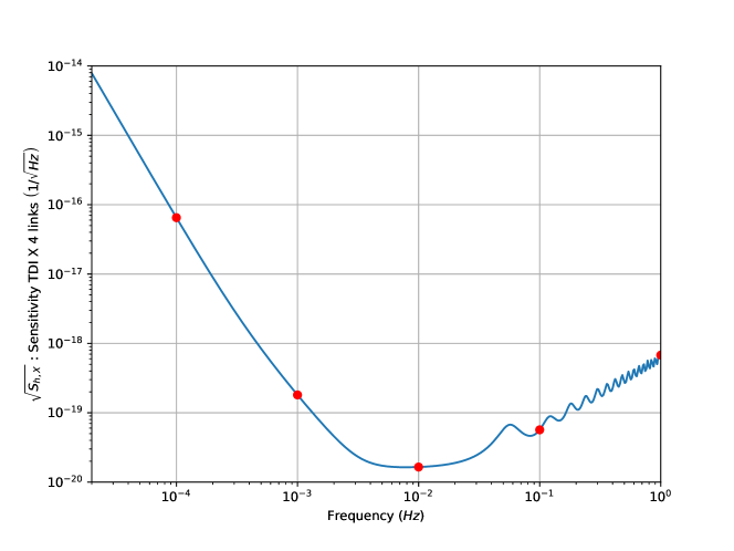
Figure 8: Sensitivity curve for a single TDI-X observable. The plot also includes the points tabulated in Table 3.

Frequency (Hz)	$S_{h,X}$	$S_{h}$
0.00010	4.227356e-33	2.113678e-33
0.00100	3.266037e-38	1.633019e-38
0.01000	2.719112e-40	1.359556e-40
0.10000	3.218770e-39	1.609385e-39
1.00000	4.598240e-37	2.299120e-37

Table 3: The numerical values of the strain sensitivity curve for some fixed frequencies.

The strain sensitivity to 6 links, $\sqrt{S_{h}}$, is plotted in fig. 1 and some points are tabulated in table 3.

6.2 Sensitivity of ground-based detectors

We start with a slight detour to show the sensitivity (as we have defined it) for LIGO-like detectors. The LIGO response is usually defined in the frame associated with the beam splitter and the characteristic wavelength of the GWs observed on the ground is usually larger than the size of the interferometer (for LIGO and other 3-4km detectors). So we can choose approximately an inertial frame covering the whole measuring device which simplifies the calculations. However, for the sake of comparison to LISA, we will use the “TT” (transverse-traceless) frame which can be seen as “co-moving” with the GW. In this frame the coordinate, distance between the beam splitter and the end mirrors does not change (but the proper distance does!): instead we can attribute the interaction with the GW to the blue/red shift of the laser frequency. To compute this effect one needs to integrate the propagation of laser’s photon in a field of (weak) GW: $g^{\alpha\beta}{\phi^{l}}_{,\alpha}{\phi^{l}}_{,\beta}=0$, where $g^{\alpha\beta}$ is a metric (for example $ds^{2}=-dt^{2}+[1+h_{+}(t-z)]dx^{2}+[1-h_{+}(t-z)]dy^{2}+dz^{2}$ is the metric of a GW propagating in $z$-direction and which has only $+$-polarization) and $\phi^{l}$ is the phase of the laser light. We can compute the phase shift after the light has traveled from the beam splitter to the end-mirrors (located along $x$ and $y$ axis) and back to the beam splitter (round trip):

$$\Delta\phi^{l}=\phi^{l}|_{x}-\phi^{l}|_{y}=-\nu_{l}\left[-2(L_{x}-L_{y})+\frac{1}{2}H(t-2L_{x})+\frac{1}{2}H(t-2L_{y})-H(t)\right]$$ (44)

where $\nu_{l}$ is the laser nominal frequency, $H(t)=\int_{0}^{t}h(t^{\prime})dt^{\prime}$ and $L_{x},L_{y}$ are coordinate distances from the beam splitter to the end mirrors, and in case of LIGO/Virgo $L_{x}=L_{y}=L$ (see details in [19]). Note that this expression does not require the long wavelength approximation $\omega L\ll 1$, but it is the case for the GW sources observed on the ground so we have

$$\Delta\phi^{l}\approx 2\nu_{l}Lh_{+}(t)$$ (45)

which allows us to define the GW strain (for GW propagating in arbitrary direction and not necessarily linearly polarized):

$$h(t)=\frac{\Delta\phi^{l}}{2\nu_{l}L}=\frac{1}{2}(n^{(1)}_{i}n^{(1)}_{j}-n^{(2)}_{i}n^{(2)}_{i})h^{ij}\equiv F_{+}h_{+}+F_{\times}h_{\times},$$ (46)

where the factor half accounts for the round trip. If we assume that $h_{+,\times}$ above is defined in the source frame then the antenna function takes the form:

$$F_{+}=-\frac{1}{2}(1+\cos^{2}\theta)\cos{2\phi}\cos{2\psi}-\cos{\theta}\sin{2\phi}\sin{2\psi}$$ (47)

$$F_{\times}=\frac{1}{2}(1+\cos^{2}\theta)\cos{2\phi}\sin{2\psi}-\cos{\theta}\sin{2\phi}\cos{2\psi}$$ (48)

We use the convention of the LISA Data Challenge (LDC).

Now we compute the square of SNR for the monochromatic source:

$$SNR^{2}=4\operatorname{Re}\left(\int_{0}^{f_{\rm max}}\,df\frac{|\tilde{h}(f)|^{2}}{S_{n}(f)}\right)$$ (49)

and average it over the sky (uniform in $\phi,\,\cos{\theta}$) and over the polarization (uniform), taking into account that $<F_{+}F_{\times}>=0$ and $<F_{+}^{2}>=<F_{\times}^{2}>=1/5$:

$$<SNR^{2}>=4\operatorname{Re}\left(\int_{0}^{f_{\rm max}}\,df\frac{\frac{1}{5}[\tilde{h}_{+}^{2}(f)+\tilde{h}_{\times}^{2}(f)]}{S_{n}(f)}\right).$$ (50)

Interestingly, in LIGO/Virgo, the numerical factor $1/5$ is usually absorbed into the signal keeping $S_{h}=S_{n}$. However according to our definition (7), $S_{h}(f)=5S_{n}(f)$, so we differ by a constant factor from the LIGO usual $S_{h}$. One needs to be careful when putting LIGO and LISA sensitivity on the sample plot! The reason for keeping this factor in the numerator is that we can also average over the inclination and define the sensitivity as the characteristic amplitude of the sky, polarization, inclination averaged monochromatic source which produces SNR=$1$ at a given frequency.

6.3 LISA sensitivity in the long wavelength limit

Now we are ready to derive the sensitivity for LISA at low frequencies ($\omega L\ll 1$). We assume only 4 links and use only X-TDI (analogue of the Michelson interferometer). The single link response in the long wavelength limit is

$$y\approx-\frac{L}{2}n_{rs}^{i}n_{rs}^{j}\dot{h}_{ij}(t-\hat{k}\vec{R}),$$ (51)

where the dot denotes the time derivative. For $X_{1.5}$ TDI in the long wavelength limit we obtain

$${X}_{1.5}\approx 2L^{2}(n_{12}^{i}n_{12}^{j}-n_{13}^{i}n_{13}^{j})\ddot{h}_{ij}.$$ (52)

It is convenient to switch to the LISA-based frame (the source sky position and polarization vary in time) where we can write:

$$\tilde{X}_{1.5}\approx(4\omega L)\sin{\omega L}\frac{\sqrt{3}}{2}(F_{+}\tilde{h}_{+}+F_{\times}\tilde{h}_{\times}),$$ (53)

where $\sqrt{3}/2$ comes from $\sin{(\pi/3)}$ - the angle between links and $F_{+,\times}$ are the antenna functions defined in the previous subsection. Finally we get for the average SNR:

$$<SNR^{2}>=4\operatorname{Re}\left(\int_{0}^{f_{\rm max}}(4\omega L)^{2}\sin^{2}({\omega L})\frac{3}{20}\frac{\tilde{h}_{+}^{2}(f)+\tilde{h}_{\times}^{2}(f)}{S_{n,X_{1.5}}(f)}\,df\right).$$ (54)

This result of averaging is the same in moving or static LISA. The sensitivity at low frequencies ($\omega L\ll 1$):

$$S_{h,X_{1.5}}^{LW}(f)=\frac{20}{3}\frac{S_{n,X_{1.5}}(f)}{(4\omega L)^{2}\sin^{2}({\omega L})},$$ (55)

where $S_{n,X_{1.5}}$ is the noise PSD given by expression (19) and this sensitivity corresponds to 4 links only (need additional factor 2 for 6-links SNR, in other words we have $10/3$ factor for 6 links). One can get a very good approximation to the numerical sensitivity with the help of an additional factor:

$$S_{h,X_{1.5}}(f)\approx\frac{20}{3}\left(1+0.6(\omega L)^{2}\right)\frac{S_{n,X_{1.5}}(f)}{(4\omega L)^{2}\sin^{2}({\omega L})},$$ (56)

and similarly for TDI $X_{2.0}$

$$S_{h,X_{2.0}}(f)\approx\frac{20}{3}\left(1+0.6(\omega L)^{2}\right)\frac{S_{n,X_{2.0}}(f)}{(4\omega L)^{2}\sin^{2}({\omega L})(2\sin{(2\omega L)})^{2}}.$$ (57)

7 Computing the SNR for black hole binaries

We start with the definition of the waveform for inspiralling binaries in the frequency domain. This covers Black Hole Binaries (BHB) with sufficient frequency evolution.

7.1 Stationary phase approximation waveform

In this subsection we will deal with the leading order Stationary Phase Approximation (SPA) waveform, defined as:

$$\tilde{h}_{+}(f) = A\frac{M_{c}^{5/6}}{D_{L}}\frac{(1+\cos^{2}{\iota})}{2}f^{-7/6}e^{i\Psi(f)},$$

$$\tilde{h}_{\times}(f) = iA\frac{M_{c}^{5/6}}{D_{L}}\cos{\iota}f^{-7/6}e^{i\Psi(f)},$$ (58)

where the chirp mass in the observer frame and amplitude are given by

$$M_{c}=M\eta^{3/5}=\frac{(m_{1}m_{2})^{3/5}}{(m_{1}+m_{2})^{1/5}},\;\;\;A=\frac{2}{\pi^{2/3}}\sqrt{\frac{5}{96}}.$$

In addition: $D_{L}$ is the luminosity distance, $\iota$ is inclination of the orbital angular momentum of the source to the line of sight, and, $\Psi(f)$ is the phase in the frequency domain which we will not need here. This corresponds to the waveform in time domain

$$h_{+}(t) = \frac{2M_{c}^{5/3}}{D_{L}}(\pi f_{\rm GW})^{2/3}(1+\cos^{2}{\iota})\cos{\Phi(t)},$$ (59)

$$h_{\times}(t) = \frac{2M_{c}^{5/3}}{D_{L}}(\pi f_{\rm GW})^{2/3}2\cos{\iota}\sin{\Phi(t)}.$$ (60)

with $f_{\rm GW}$, the frequency of GW in the observer frame (twice the orbital frequency).

NOTE: Very often the amplitude of cross-polarization is defined with opposite sign!

We have neglected higher order modes considering only the leading order ($2,\pm 2$), and we consider non-precessing binaries. Moreover, the expressions (58) are valid only for early inspiral.

Another way of writing two polarizations of GWs is via mode decomposion (decomposition in spin-weighted spherical harmonics) defined as:

$$\tilde{h}_{+} = \frac{1}{2}\sum_{l\leq 2}\sum_{m=-l}^{l}Y^{(-2)}_{lm}\tilde{h}_{lm}+Y^{*(-2)}_{lm}\tilde{h}^{*}_{lm}(-f),$$ (61)

$$\tilde{h}_{\times} = \frac{i}{2}\sum_{l\leq 2}\sum_{m=-l}^{l}Y^{(-2)}_{lm}\tilde{h}_{lm}-Y^{*(-2)}_{lm}\tilde{h}^{*}_{lm}(-f).$$ (62)

The advantage of this form is that the angular dependence of gravitational radiation is absorbed in the spherical harmonics. If there is no precession (the case which we consider here), $h_{l,-m}=(-1)^{l}h^{*}_{lm}$. We will consider here only the dominant harmonic ($l=2,m=\pm 2$), so that

$$\tilde{h}_{22}=A_{22}e^{i\Psi},\;\;\;\;\tilde{h}_{2-2}=A_{22}e^{-i\Psi}.$$

The two polarizations in this case (for positive frequencies) are

$$\tilde{h}_{+} = \frac{1}{2}\left(Y_{22}+Y^{*}_{2-2}\right)A_{22}e^{i\Psi},$$ (63)

$$\tilde{h}_{\times} = \frac{i}{2}\left(Y_{22}-Y^{*}_{2-2}\right)A_{22}e^{i\Psi}.$$ (64)

Note that those expressions are more general (we did not specify $A_{22}(f)$, $\Psi(f)$) and applicable also to the leading harmonic of phenomenological IMR (Inspiral-Merger-Ringdown) waveforms.

7.1.1 SNR averaged over sky, polarization and inclination of a coalescing binary

A quantity often used in LISA to assess the scientific performance is the SNR of a binary system defined by intrinsic parameters (masses, spins) and distance but on average over sky, polarization and inclination.

In case of the ground-based detectors the SNR is computed as

$$SNR^{2}=4\operatorname{Re}\left(\int_{0}^{f_{\textrm{max}}}\frac{\tilde{h}(f)\tilde{h}^{*}(f)}{S_{n}(f)}df\right),$$ (65)

where $\tilde{h}(f)$ is given by LIGO-type strain (46) and $S_{n}(f)$ is the noise (or sensitivity, again, in LIGO-sense). We can average $|\tilde{h}(f)|^{2}$ over inclination, polarization and sky analytically. Introduce an angle between two arms as $\gamma$ ($\gamma=\pi/2$ for LIGO-like detectors and $\gamma=\pi/3$ for LISA and ET) and consider a single Michelson measurement ($X$ only in case of LISA). The averaging procedure implies

$$<|\tilde{h}(f)|^{2}>_{\iota,\psi,\rm sky}=\frac{1}{4\pi}\int\,d^{2}\Omega\frac{1}{2\pi}\int_{0}^{2\pi}\,d\psi\frac{1}{2}\int_{-1}^{1}\,d\cos(\iota)|\tilde{h}(f)|^{2}$$ (66)

Introduce polarization-dependent amplitudes $a_{+}=(1+\cos^{2}{\iota})/2,\,\,a_{\times}=\cos{\iota}$ then the averaging procedure applied to $\tilde{h}=F_{+}\tilde{h}_{+}(f)+F_{\times}\tilde{h}_{\times}(f)$ implies

$$\left<(F_{+}a_{+})^{2}+(F_{\times}a_{\times})^{2}\right>_{\iota,\psi,\rm sky}=\frac{4}{25}\sin^{2}{\gamma}$$ (67)

and for SPA gives

$$\left<\tilde{h}(f)\right>_{\rm LIGO} = \frac{1}{\sqrt{30}}\frac{M_{c}^{5/6}}{\pi^{2/3}D_{L}}f^{-7/6}e^{i\Psi(f)}.$$ (68)

$$\left<\tilde{h}(f)\right>_{\textrm{LISA}} = \frac{1}{2\sqrt{10}}\frac{M_{c}^{5/6}}{\pi^{2/3}D_{L}}f^{-7/6}e^{i\Psi(f)}.$$ (69)

Similar averaging procedure applied to phenomenological waveform restricted to $(2,\pm 2)$ mode only

$$h_{+} = \sqrt{\frac{5}{64\pi}}e^{2i\phi_{0}}(1+\cos^{2}{\iota})A_{22}(f)e^{i\Psi(f)},$$ (70)

$$h_{\times} = i\sqrt{\frac{5}{64\pi}}e^{2i\phi_{0}}2\cos{\iota}A_{22}(f)e^{i\Psi(f)},$$ (71)

gives us

$$\left<\tilde{h}(f)\right>_{\textrm{LISA}}=\frac{1}{2}\sqrt{\frac{3}{20\pi}}A_{22}(f)e^{i\Psi(f)}.$$ (72)

Another used quantity is the SNR of the optimally oriented source, implying that the inclination is $\cos{\iota}=1$ which maximizes $a_{+,\times}=1$. The averaging over the sky and polarization for the face-on source gives

$$\textrm{max}_{\iota}\left<(F_{+}a_{+})^{2}+(F_{\times}a_{\times})^{2}\right>_{\psi,\rm sky}=\frac{2}{5}\sin^{2}{\gamma}.$$ (73)

Return back to SNR. In case of LISA we have

$$<SNR^{2}_{X}>=4\operatorname{Re}\left(\int_{0}^{f_{\textrm{max}}}(4\omega L)^{2}\sin^{2}({\omega L})<(F_{X}^{+})^{2}>\frac{\tilde{h}_{+}^{2}(f)+\tilde{h}_{\times}^{2}(f)}{S_{n,X_{1.5}}(f)}\,df\right)=4\operatorname{Re}\left(\int_{0}^{f_{\textrm{max}}}\frac{\tilde{h}_{+}^{2}(f)+\tilde{h}_{\times}^{2}(f)}{S_{h,X}(f)}\,df\right).$$ (74)

What is left is to average the expression above over inclination, for a simple case of a dominant harmonic $|\tilde{h}_{+,\times}|=a_{+,\times}A(f)$ we have:

$$<SNR^{2}_{X}>_{\iota,\psi,\rm sky}=4\operatorname{Re}\left(\int_{0}^{f_{\textrm{max}}}<a_{+}^{2}+a_{\times}^{2}>_{\iota}\frac{A^{2}(f)}{S_{h,X}(f)}\,df\right)=4\operatorname{Re}\left(\int_{0}^{f_{\textrm{max}}}\frac{\frac{4}{5}A^{2}(f)}{S_{h,X}(f)}\,df\right).$$ (75)

In the long wavelength approximation and for SPA this translates into

$$\left<SNR_{X}^{2}\right>_{\iota,\psi,\rm sky}=4\operatorname{Re}\left(\int_{0}^{f_{\rm{max}}}\frac{\sin^{2}{\gamma}<F^{2}_{+}a^{2}_{+}+F^{2}_{\times}a^{2}_{\times}>_{\psi,\iota,\rm{sky}}}{\sin^{2}{\gamma}<F^{2}_{+}>_{\psi,\rm sky}S^{LW}_{h,X}(f)}\left(A\frac{M_{c}^{5/6}}{D_{L}}\right)^{2}f^{-7/3}\,df\right)$$ (76)

where $S^{LW}_{h,X}$ is given by eqn. (56). The term in the numerator is just $\left<\tilde{h}(f)\right>$ given above and the factor $\sin^{2}{\gamma}<F^{2}_{+}>_{\psi,\rm sky}$ (which is 3/20 in case of LISA) is often referred as “de-averaging” factor. We can get a similar expression for a single mode of PhenomIMR waveforms. Finally the combined SNR for LISA is obtained by $\left<SNR^{2}\right>_{\iota,\psi,\rm sky}=2\left<SNR_{X}^{2}\right>_{\iota,\psi,\rm sky}$ or replacing $S_{h,X}(f)$ by $S_{h}(f)$ in denominator.

In the Appendix C we compute SNR for several reference MBHBs systems using eq. (76) and three phenomenological IMR models: PhenomA, PhenomC, PhenomD, those models perform similarly for equal mass non-spinning systems but could give very different results as we increase mass ratio and spins. This is expected: PhenomD [8] supersedes PhenomC and PhenomA as it was built based on the extended set of numerical waveforms (up to mass ratio 16).

8 Relation of the sensitivity to SNR

To answer if and how the sensitivity $S_{h}(f)$ is connected to the SNR, we consider a monochromatic GW source given in time domain by two polarizations in the source frame:

$$h_{+}(t) = h_{0}\frac{1+\cos^{2}{\iota}}{2}\cos(\omega_{0}t+\phi_{0})$$ (77)

$$h_{\times}(t) = h_{0}\cos{\iota}\cos(\omega_{0}t+\phi_{0})$$ (78)

While transforming to the frequency domain we (i) consider only positive frequencies (ii) neglect harmonics which appear due to relative motion of the source and the detector (relevant for LISA) which leads to :

$$\tilde{h}_{+}(f) = \frac{1}{2}h_{0}\frac{1+\cos^{2}{\iota}}{2}e^{i\phi_{0}}\delta_{T}(f-f_{0}),$$ (79)

$$\tilde{h}_{\times}(f) = \frac{-i}{2}h_{0}\cos{\iota}e^{i\phi_{0}}\delta_{T}(f-f_{0}),$$ (80)

where the delta function should be understood in reality as a finite time approximation $\delta_{T}(f-f_{0})\approx T\textrm{Sinc}\left[T(f-f_{0})\right]$ and $T$ is the observation duration. We will use again the SNR in LIGO-sense as described by (76). For LIGO-like detectors which use $S_{h}^{\rm LIGO}(f)=S_{n}(f)$ as the sensitivity we obtain

$$\left<SNR_{X}^{2}\right>_{\iota,\psi,\rm sky}=\frac{<F^{2}_{+}A^{2}_{+}+F^{2}_{\times}A^{2}_{\times}>_{\psi,\iota,\rm{sky}}}{S_{h}^{\rm LIGO}(f)}h_{0}^{2}T=\frac{\left(\frac{2}{5}h_{0}\right)^{2}T}{S_{h}^{\rm LIGO}(f)},$$ (81)

This says, that $\sqrt{S_{h}^{\rm LIGO}(f)}$ can be interpreted as the amplitude of polarization, inclination and sky averaged monochromatic GW signal which gives $SNR=1$ after observing it for $T_{\rm obs}=T$ with a single detector.

Let us try to interprete LISA sensitivity in a similar way. We consider static LISA and use (76) taking into account that

$$<F^{2}_{+}a^{2}_{+}+F^{2}_{\times}a^{2}_{\times}>_{\psi,\iota,\rm{sky}}=\frac{4}{25}\sin^{2}\gamma$$ (82)

$$<F^{2}_{+}>_{\psi,\rm sky}=<F^{2}_{\times}>_{\psi,\rm sky}=\frac{1}{5}\sin^{2}\gamma$$ (83)

we obtain for sensitvity (combined out of two noise independent data streams):

$$\left<SNR^{2}\right>_{\iota,\psi,\rm sky}=\frac{<F^{2}_{+}a^{2}_{+}+F^{2}_{\times}a^{2}_{\times}>_{\psi,\iota,\rm{sky}}}{<F^{2}_{+}>_{\psi,\rm sky}S_{h}(f)}\left(h_{0}^{2}T\right)^{2}=5\frac{\left(\frac{2}{5}h_{0}\right)^{2}T}{S_{h}(f)},$$ (84)

Clearly it has different interpretations: (combined) LISA sensitivity $\sqrt{S_{h}(f)}$ can be seen as the amplitude of polarization, inclination and sky averaged monochromatic GW signal which gives a combined $SNR^{2}=5$ after observing it for $T_{\rm obs}=T$. We should however emphasize that we have defined “polarization, inclination and sky averaged monochromatic GW signal” excluding the factor $\sin^{2}{(\gamma)}$ for comparison with the ground-based GW detectors. If we include the angle between the arms into the definition of an average signal $\left(\sin{(\gamma)}\frac{2}{5}h_{0}\right)$, then the combined SNR should be $SNR^{2}=20/3$.

9 Galactic confusion noise

The numerical results for the Galactic confusion noise were first obtained using in [21] for several durations of observation. The level of Galactic noise is assessed by generating the simulated data which contains the Galactic population of White Dwarf (WD) binaries (based on a fiducial model [9]). The bright sources are removed in a iterative manner using smooth fit in estimated PSD (combination of the noise and GW signals). The first estimator of the PSD will be severely biased by the loud GW signals, removal of the bright sources and re-evaluation of the PSD is converging after about 8-10 iterations. As the result we have a number resolvable sources (assuming perfect removal of bright sources) and the residual stochastic foreground. NOTE that this procedure is sensitive to (i) SNR threshold assumed for identification and removal of the sources (ii) the method used to evaluate the smooth PSD (running median or mean). The fit below was obtained assuming combined SNR threshold $SNR>7$ and running mean for smoothing PSD estimator (see for details Karnesis+ [2021], in preparation).

The analytic fit expression of the strain sensitivity curve is given as

$$S_{\rm Gal}=Af^{-7/3}e^{-\left(\frac{f}{f_{1}}\right)^{\alpha}}\frac{1}{2}\left[1.0+\tanh\left(-\frac{f-f_{k}}{f_{2}}\right)\right],$$ (85)

where $A=1.14\times 10^{-44},\,\alpha=1.8,\,f_{2}=0.31\,\rm{mHz}$ and $f_{1},f_{k}$ depend on the observation time (we resolve and remove more signals for longer observation).

$$\log_{10}(f_{1})=a_{1}\log_{10}(T_{obs})+b_{1},\,\,\,\,\log_{10}(f_{k})=a_{k}\log_{10}(T_{obs})+b_{k}$$ (86)

Here $T_{obs}$ is in years and $a_{1},\,b_{1}$ are $-0.25,\,-2.7$ and $a_{k},\,b_{k}$ are $-0.27,-2.47$. The first term in this expression corresponds to what we expect (PSD) from the population of monochromatic GW sources. The second term reflects fact that we have fewer sources at high frequencies and that the bright sources are removed. The last term is determined by the data analysis: $f_{k}$ is a characteristic frequency above which we should be able to resolve and remove all GB sources.

In the figure 9 we show evolution of Galactic foreground for $(1,4,6,10)$ years of observation.

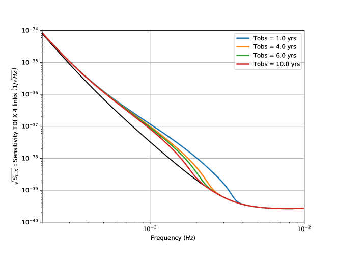
Figure 9: Analytic fits to the numerical results for estiamtion of the stochastic GW signal from the WD Galactic binaries.

10 Cosmology

This note uses the following cosmological parameters for conversion of redshift to luminosity distance. The conversion is typically done according to the description given in [7].

The parameters used are Lambda CDM taken from [16] and are quoted here:

$$\Omega_{M} = 0.3175~{}\textrm{(Matter)}$$ (87)

$$\Omega_{k} = 0~{}\textrm{(Curvature)}$$ (88)

$$\Omega_{\Lambda} = 0.6825~{}\textrm{(Density)}$$ (89)

$$h = 0.671$$ (90)

$$H_{0} = 67.1\,\textrm{km}\,\textrm{s}^{-1}\,\textrm{Mpc}^{-1}$$ (91)

With these parameters the luminosity distance corresponding to $z=1$ is $D_{L}=6823Mpc$.

11 Stochastic GW backgrounds

The quantity usually used to describe the sensitivity to SGWB is the energy density sensitivity defined by :

$$h^{2}\Omega_{Sens}(f)={4\pi^{2}\over 3H_{0}^{2}}f^{3}S_{h}(f)$$ (92)

with $H_{0}=h\ h_{0}$, $h_{0}=100\ \rm{km}\,\rm{s}^{-1}\,\rm{Mpc}^{-1}=3.24\times 10^{-18}Hz$, $h$ the reduced Hubble constant and $S_{h}(f)$ is the strain sensitvity in $Hz^{-1}$.

The figure 10 is showing the sensitivity in energy density.

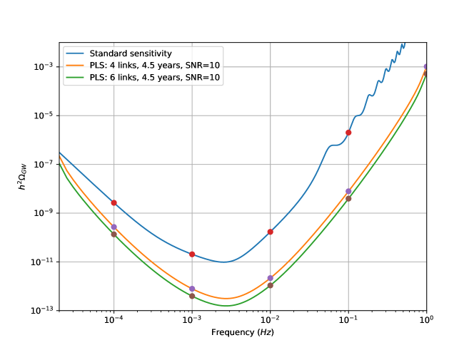
Figure 10: The sensitivity in $h^{2}\Omega_{GW}$ and PLS for 4.5 years and SNR=10. The plot also includes the points tabulated in Table 4.

The SNR of a SGWB with energy density $\Omega_{GW}(f)$ and observed for a duration $T_{obs},$ is computed by the following integration over the frequency :

$$SNR=\sqrt{T_{obs}\int_{f_{min}}^{f_{max}}df{(h^{2}\Omega_{GW}(f))^{2}\over(h^{2}\Omega_{Sens}(f))^{2}}}$$ (93)

In order to quickly estimate the detectability of a power law SGWB, i.e. in the form

$$h^{2}\Omega_{GW}(f)=\Omega_{\beta}\left({f\over f_{ref}}\right)^{\beta},$$ (94)

within the observed frequency range, i.e. $f\in[2\times 10^{-5},1]$Hz, the Power Law Sensitivity (PLS) has been introduced [20]. For an observation duration $T_{obs}$, it is computed as the enveloppe of all power law SGWB with $SNR=SNR_{thr}$, scanning the slope $\beta$ (see figure 11).

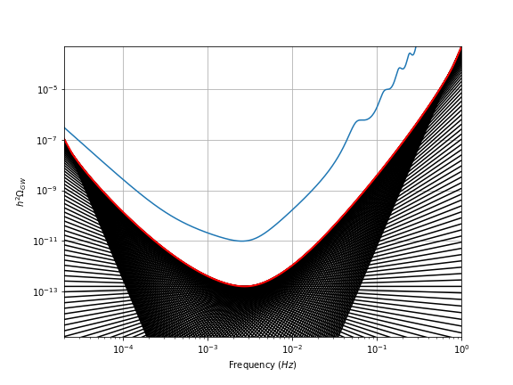
Figure 11: Computation of the PLS for 4.5 years and SNR=10 (red). The black lines are all power laws of various index with SNR=10. The plot also includes the sensitivty as reference (blue).

The use of the PLS is straightforward: if one part of a power law representing the signal is higher than the PLS, the signal is detectable.

We usually choose $SNR_{thr}=10$ (for example [6]). It is based on the preliminary results about SGWB detectability [2], adding some margin. The nominal duration of the mission is 4.5 years. The corresponding PLS is shown in the figure 10 and some points are tabulated in table 4.

Frequency (Hz)	$h^{2}\Omega_{GW}$	PLS 4 links	PLS 6 links
0.00010	2.648253e-09	2.692611e-10	1.346306e-10
0.00100	2.046074e-11	7.873148e-13	3.936574e-13
0.01000	1.703482e-10	2.160153e-12	1.080076e-12
0.10000	2.016455e-06	7.868305e-09	3.934152e-09
1.00000	2.861449e-01	1.030663e-03	5.153315e-04

Table 4: The numerical values for some fixed frequencies of the sensitivity in $h^{2}\Omega_{GW}$ and PLS for 4.5 years and SNR=20.

12 APPENDIX

Appendix A Noise PSD derivation

In this appendix, we provide a detailed computation of the noise PSD, given by formulas (17), (18), (19) and (20) above. Introduce the following assumptions:

1. no residual laser noise;

2. no clock noise;

3. no optical bench noise;

4. no backlink noise;

5. no ranging error;

6. no interpolation error;

7. no effect of on board filtering of the measurements;

8. all lasers are at the same nominal frequency, $c/\lambda$;

9. consider only the projection of the acceleration noise on the sensitive axis, $\delta_{i}$

10. all the Optical Metrology System (OMS) noises, optical path noises and readout noises are grouped in one term, $N_{ij}$, for the science interferometer; this type of noise is neglected for the other interferometers;

11. $\theta_{i}^{j}$ account for the frequency polarity :

    $$\theta_{ij}^{kl}=\left\{\begin{array}[]{cc}+1&\rm{if}\quad\omega_{kl\rightarrow ij}-\omega_{ij}>0\\ -1&\rm{if}\quad\omega_{kl\rightarrow ij}-\omega_{ij}<0\end{array}\right.\quad{\rm with}\quad\omega_{ij}=2\pi\nu_{ij}$$ (95)

with $\omega_{ij}$ the frequency of the laser on optical bench $ij$ and $\omega_{kl\rightarrow ij}$ the frequency of the beam received on optical bench $ij$ from optical bench $kl$.

The measurements on the two optical benches of spacecraft 1 are

$$\left\{\begin{array}[]{lll}s_{12}^{c}&=&\theta_{12}^{21}\ N_{12}\\ \tau_{12}&=&0\\ \epsilon_{12}&=&2\theta_{12}^{13}\ \delta_{12}\\ s_{12}^{sb}&=&\theta_{12}^{21}\ N_{12}\end{array}\right.\quad\quad\left\{\begin{array}[]{lll}s_{13}^{c}&=&\theta_{13}^{31}\ N_{13}\\ \tau_{13}&=&0\\ \epsilon_{13}&=&-2\theta_{13}^{12}\ \delta_{13}\\ s_{13}^{sb}&=&\theta_{13}^{31}\ N_{13}\end{array}\right.$$ (96)

We then apply the first step of TDI to suppress the spacecraft jitter

$$\xi_{12} = s_{12}^{c}-\theta_{12}^{21}\theta_{12}^{13}{\epsilon_{12}-\tau_{12}\over 2}-\theta_{12}^{21}\theta_{21}^{23}{D_{12}\epsilon_{21}-D_{12}\tau_{21}\over 2}$$

$$= \theta_{12}^{21}N_{12}-\theta_{12}^{21}\theta_{12}^{13}\theta_{12}^{13}\delta_{12}-\theta_{12}^{21}\theta_{21}^{23}D_{12}(-\theta_{21}^{23}\delta_{21})$$

$$\xi_{12} = \theta_{12}^{21}\left(N_{12}-\delta_{12}+D_{12}\delta_{21}\right)$$ (98)

$$\xi_{13} = s_{13}^{c}-\theta_{13}^{31}\theta_{13}^{12}{\epsilon_{13}-\tau_{13}\over 2}-\theta_{13}^{31}\theta_{31}^{32}{D_{13}\epsilon_{3}-D_{13}\tau_{31}\over 2}$$

$$= \theta_{13}^{31}N_{13}-\theta_{13}^{31}\theta_{13}^{12}(-\theta_{13}^{12}\delta_{13})-\theta_{13}^{31}\theta_{31}^{32}D_{13}\theta_{31}^{32}\delta_{31}$$

$$\xi_{13} = \theta_{13}^{31}\left(N_{13}+\delta_{13}-D_{13}\delta_{31}\right)$$ (100)

Then we reduce half of the laser noise, i.e. equivalent to one laser per spacecraft (see section 4.3.3 of [13]):

$$\eta_{12} = \theta_{12}^{21}\xi_{12}+{\theta_{23}^{21}D_{12}\tau_{21}-\theta_{21}^{23}D_{12}\tau_{23}\over 2}$$ (101)

$$= N_{12}-\delta_{12}+D_{12}\delta_{21}$$

$$\eta_{13} = \theta_{13}^{31}\xi_{13}-{\theta_{13}^{12}\tau_{13}-\theta_{12}^{13}\tau_{12}\over 2}$$ (102)

$$= N_{13}+\delta_{13}-D_{13}\delta_{31}$$

Now he have to apply the TDI generators. We use TDI generator X (Michelson) as for the sensitivity curve, and TDI-generation 1.5 is given as

$$X_{1.5} = \eta_{13}+D_{13}\eta_{31}+D_{13}D_{31}\eta_{12}+D_{13}D_{31}D_{12}\eta_{21}-\eta_{12}-D_{12}\eta_{21}-D_{12}D_{21}\eta_{13}-D_{12}D_{21}D_{13}\eta_{31}$$ (103)

$$= N_{13}+\delta_{13}-D_{13}\delta_{31}$$

$$+D_{13}N_{31}-D_{13}\delta_{31}+D_{13}D_{31}\delta_{13}$$

$$+D_{13}D_{31}N_{12}-D_{13}D_{31}\delta_{12}+D_{13}D_{31}D_{12}\delta_{21}$$

$$+D_{13}D_{31}D_{12}N_{21}+D_{13}D_{31}D_{12}\delta_{21}-D_{13}D_{31}D_{12}D_{21}\delta_{12}$$

$$-N_{12}+\delta_{12}-D_{12}\delta_{21}$$

$$-D_{12}N_{21}-D_{12}\delta_{21}+D_{12}D_{21}\delta_{12}$$

$$-D_{12}D_{21}N_{13}-D_{12}D_{21}\delta_{13}+D_{12}D_{21}D_{13}\delta_{31}$$

$$-D_{12}D_{21}D_{13}N_{31}+D_{12}D_{21}D_{13}\delta_{31}-D_{12}D_{21}D_{13}D_{31}\delta_{13}$$

Factorizing, we get:

$$X_{1.5} = (1-D_{12}D_{21})N_{13}-(1-D_{13}D_{31})N_{12}+(D_{13}-D_{12}D_{21}D_{13})N_{31}-(D_{12}-D_{13}D_{31}D_{12})N_{21}$$ (104)

$$(1+D_{12}D_{21}-D_{13}D_{31}-D_{13}D_{31}D_{12}D_{21})\delta_{12}+(1-D_{12}D_{21}+D_{13}D_{31}-D_{12}D_{21}D_{13}D_{31})\delta_{13}$$

$$-2(D_{12}-D_{13}D_{31}D_{12})\delta_{21}-2(D_{13}-D_{12}D_{21}D_{13})\delta_{31}$$

The next step is the computation of PSD. Note that

$$PSD\left[(1-D_{13}D_{31})N_{12}\right] = \left\langle\left(1-e^{-i\omega(L_{13}+L_{31})}\right)\left(1-e^{i\omega(L_{13}+L_{31})}\right)\tilde{N}_{12}\tilde{N}_{12}^{*}\right\rangle$$ (105)

$$= \left\langle\left(e^{i\omega{L_{13}+L_{31}\over 2}}-e^{-i\omega{L_{13}+L_{31}\over 2}}\right)\tilde{N}_{12}\tilde{N}_{12}^{*}\right\rangle$$

$$= 4\sin^{2}\left(\omega{L_{13}+L_{31}\over 2}\right)S_{OMS_{12}},$$

so the PSD of terms 1, 2, 3, 4, 7 and 8 can be reduced in a similar way. The tilde denotes the Fourier transfer of the quantity. The term 5 and 6 are given by:

$$PSD[(1+D_{12}D_{21}-D_{13}D_{31}-D_{13}D_{31}D_{12}D_{21})\delta_{12}]$$ (106)

$$= \left\langle\left(1+e^{-i\omega(L_{12}+L_{21})}-e^{-i\omega(L_{13}+L_{31})}-e^{-i\omega(L_{13}+L_{31}+L_{12}+L_{21})}\right)\left(...\right)^{*}\tilde{\delta}_{12}\tilde{\delta}_{12}^{*}\right\rangle$$

$$= \left\langle\left(\left(1+e^{-i\omega(L_{12}+L_{21})}\right)\left(1-e^{-i\omega(L_{13}+L_{31})}\right)\right)\left(...\right)^{*}\tilde{\delta}_{12}\tilde{\delta}_{12}^{*}\right\rangle$$

$$= \left\langle\left(e^{i\omega{L_{12}+L_{21}\over 2}}+e^{-i\omega{L_{12}+L_{21}\over 2}}\right)^{2}\left(e^{i\omega{L_{13}+L_{31}\over 2}}-e^{-i\omega{L_{13}+L_{31}\over 2}}\right)^{2}\delta_{12}\delta_{12}^{*}\right\rangle$$

$$= 16\cos^{2}\left(\omega{L_{12}+L_{21}\over 2}\right)\sin^{2}\left(\omega{L_{13}+L_{31}\over 2}\right)S_{acc_{12}}.$$

Similarly we can write the 2nd generation $X$-TDI:

$$X_{2.0} = \eta_{13}+D_{13}\eta_{31}+D_{13}D_{31}\eta_{12}+D_{13}D_{31}D_{12}\eta_{21}+D_{13}D_{31}D_{12}D_{21}\eta_{12}$$ (107)

$$+D_{13}D_{31}D_{12}D_{21}D_{12}\eta_{21}+D_{13}D_{31}D_{12}D_{21}D_{12}D_{21}\eta_{13}+D_{13}D_{31}D_{12}D_{21}D_{12}D_{21}D_{13}\eta_{31}$$

$$-\eta_{12}-D_{12}\eta_{21}-D_{12}D_{21}\eta_{13}-D_{12}D_{21}D_{13}\eta_{31}-D_{12}D_{21}D_{13}D_{31}\eta_{13}$$

$$-D_{12}D_{21}D_{13}D_{31}D_{13}\eta_{31}-D_{12}D_{21}D_{13}D_{31}D_{13}D_{31}\eta_{12}-D_{12}D_{21}D_{13}D_{31}D_{13}D_{31}D_{12}\eta_{21}$$

$$= (1-D_{12}D_{21}D_{13}D_{31})((\eta_{13}+D_{13}\eta_{31})+D_{13}D_{31}(\eta_{12}+D_{12}\eta_{21}))$$

$$-(1-D_{13}D_{31}D_{12}D_{21})((\eta_{12}+D_{12}\eta_{21})+D_{12}D_{21}(\eta_{13}+D_{13}\eta_{31}))$$

$$= (1-D_{12}D_{21}D_{13}D_{31})((N_{13}+D_{13}N_{31}+(1+D_{13}D_{31})\delta_{13}-2D_{13}\delta_{31})$$

$$+D_{13}D_{31}(N_{12}+D_{12}N_{21}-\delta_{12}(1+D_{12}D_{21})+2D_{12}\delta_{21}))$$

$$-(1-D_{13}D_{31}D_{12}D_{21})((N_{12}+D_{12}N_{21}-(1+D_{12}D_{21})\delta_{12}+2D_{12}\delta_{21})$$

$$+D_{12}D_{21}(N_{13}+D_{13}N_{31}+(1+D_{13}D_{31})\delta_{13}-2D_{13}\delta_{31})).$$

Factorizing, we get:

$$X_{2.0} = (1-D_{12}D_{21}D_{13}D_{31})((1-D_{12}D_{21})(N_{13}+D_{13}N_{31}+(1+D_{13}D_{31})\delta_{13}-2D_{13}\delta_{31})$$ (108)

$$-(1-D_{13}D_{31})(N_{12}+D_{12}N_{21}-(1+D_{12}D_{21})\delta_{12}+2D_{12}\delta_{21}))$$

Approximation: Armlength are constant, i.e. the delay operators are commuting.

$$PSD_{X_{1.5}} = 4\sin^{2}\left(\omega{L_{31}+L_{13}\over 2}\right)\left(S_{OMS_{12}}+S_{OMS_{21}}+4S_{acc_{21}}+4\cos^{2}\left(\omega{L_{12}+L_{21}\over 2}\right)S_{acc_{12}}\right)$$ (109)

$$+4\sin^{2}\left(\omega{L_{21}+L_{12}\over 2}\right)\left(S_{OMS_{13}}+S_{OMS_{3}}+4S_{acc_{3}}+4\cos^{2}\left(\omega{L_{31}+L_{13}\over 2}\right)S_{acc_{13}}\right)$$

Computation of PSD for the 2nd generation TDI requires some additional math. Starting with

$$PSD_{X_{2.0}} = \left\langle\left[\left(1-e^{-i\omega(L_{12}+L_{21}+L_{13}+L_{31})}\right)\right.\right.$$

$$\times\left(\left(1-e^{-i\omega(L_{12}+L_{21})}\right)\left(\tilde{N}_{13}+e^{-i\omega L_{13}}\tilde{N}_{31}+\left(1+e^{-i\omega(L_{13}+L_{31})}\right)\tilde{\delta}_{13}-2e^{-i\omega L_{13}}\tilde{\delta}_{31}\right)\right.$$

$$\left.\left.\left.-\left(1-e^{-i\omega(L_{13}+L_{31})}\right)\left(\tilde{N}_{12}+e^{-i\omega L_{12}}\tilde{N}_{21}-\left(1+e^{-i\omega(L_{12}+L_{21})}\right)\tilde{\delta}_{12}+2e^{-i\omega L_{12}}\tilde{\delta}_{21}\right)\right)\right][...]^{*}\right\rangle$$

and using the following simplifications

$$\left(1-e^{-i\omega(L_{12}+L_{21}+L_{13}+L_{31})}\right)(...)^{*} \rightarrow 4\sin^{2}\left(\omega\frac{L_{12}+L_{21}+L_{13}+L_{31}}{2}\right)$$

$$\left(1-e^{-i\omega(L_{12}+L_{21})}\right)(...)^{*} \rightarrow 4\sin^{2}\left(\omega\frac{L_{12}+L_{21}}{2}\right)$$

$$\left(1+e^{-i\omega(L_{12}+L_{21})}\right)(...)^{*} \rightarrow 4\cos^{2}\left(\omega\frac{L_{12}+L_{21}}{2}\right)$$

$$\left(e^{-i\omega L_{12}}\right)(...)^{*} \rightarrow 1$$

we arrive at

$$PSD_{X_{2.0}} = 16\sin^{2}\left(\omega\frac{L_{12}+L_{21}+L_{13}+L_{31}}{2}\right)$$ (111)

$$\times\left(\sin^{2}\left(\omega\frac{L_{12}+L_{21}}{2}\right)\left(S_{OMS_{13}}+S_{OMS_{31}}+4\left(S_{acc_{31}}+\cos^{2}\left(\omega\frac{L_{13}+L_{31}}{2}\right)S_{acc_{13}}\right)\right)\right.$$

$$\left.+\sin^{2}\left(\omega\frac{L_{13}+L_{31}}{2}\right)\left(S_{OMS_{12}}+S_{OMS_{21}}+4\left(S_{acc_{21}}+\cos^{2}\left(\omega\frac{L_{12}+L_{21}}{2}\right)S_{acc_{12}}\right)\right)\right).$$

Approximation 1+2: Armlength are all equal.

$$S_{n,X_{1.5}}=PSD_{X_{1.5}}=4\sin^{2}\left(\omega L\right)\left(S_{OMS_{12}}+S_{OMS_{21}}+S_{OMS_{13}}+S_{OMS_{31}}+\right.$$

$$\left.4\left(S_{acc_{21}}+S_{acc_{31}}+\cos^{2}\left(\omega L\right)\left(S_{acc_{12}}+S_{acc_{13}}\right)\right)\right)$$

$$PSD_{X_{2.0}} = 16\sin^{2}\left(2\omega L\right)\sin^{2}\left(\omega L\right)\left(S_{OMS_{13}}+S_{OMS_{31}}+S_{OMS_{12}}+S_{OMS_{21}}\right.$$ (112)

$$\left.+4\left(S_{acc_{31}}+S_{acc_{21}}+\cos^{2}\left(\omega L\right)\left(S_{acc_{13}}+S_{acc_{12}}\right)\right)\right)$$

Approximation 1+2+3: All noises of the same type have the same PSD ($S_{OMS_{ij}}=S_{OMS}$ and $S_{acc_{ij}}=S_{acc}$):

$$S_{n,X_{1.5}}=PSD_{X_{1.5}}=16\sin^{2}\left(\omega L\right)\left(S_{OMS}+\left(3+\cos\left(2\omega L\right)\right)S_{acc}\right)$$

$$PSD_{X_{2.0}} = 64\sin^{2}\left(2\omega L\right)\sin^{2}\left(\omega L\right)\left(S_{OMS}+2\left(1+\cos^{2}\left(\omega L\right)\right)S_{acc}\right)$$ (113)

$$= 64\sin^{2}\left(2\omega L\right)\sin^{2}\left(\omega L\right)\left(S_{OMS}+\left(3+\cos\left(2\omega L\right)\right)S_{acc}\right)$$

Appendix B Noise spectrum from SciRD sensitivity

The official required sensitivity of LISA is decribed in [12]:

$$S_{h,SciRD}(f) = \frac{1}{2}\frac{20}{3}\left(\frac{S_{I}(f)}{(2\pi f)^{4}}+S_{II}(f)\right)R(f)$$

$$S_{I}(f) = 5.76\times 10^{-48}\left(1+\left(\frac{f_{1}}{f}\right)^{2}\right)\textrm{s}^{-4}.\textrm{Hz}^{-1}$$ (114)

$$S_{II}(f) = 3.6\times 10^{-41}\textrm{Hz}^{-1}$$

$$R(f) = 1+\left(\frac{f}{f_{2}}\right)^{2}$$

with $f_{1}=0.4\textrm{mHz}$ and $f_{2}=25\textrm{mHz}$. It is for a full instrument so 6 links.

The analytic approximation of the sensitivity for TDI $X_{2.0}$ (4 links) is given by equation (57). By equalizing the sensitivities, i.e. $S_{h,SciRD}=S_{h,X_{2.0}}/2$ and using $R(f)\approx 1+0.6(\omega L)^{2}$, we get for the noise PSD in relative frequency (as $S_{n,X_{2.0}}$ is in relative frequency in (57)):

$$S_{n,X_{2.0}} \approx (4\omega L)^{2}\sin^{2}({\omega L})(2\sin{(2\omega L)})^{2}\left(\frac{S_{I}(\omega)}{\omega^{4}}+S_{II}(\omega)\right)$$ (115)

Converting to displacement (i.e. divide by $(\omega/c)^{2}$):

$$S_{n,X_{2.0},dL} \approx 4C(\omega)\left(\frac{S_{I}(\omega)}{\omega^{4}}L^{2}+S_{II}(\omega)L^{2}\right)$$ (116)

with

$$C(\omega) = 16\sin^{2}({\omega L})\sin^{2}{(2\omega L)})$$ (117)

We find back the values for the two noise terms (see 3):

$$S_{oms}(\omega) = S_{II}(\omega)L^{2}=\left(15\ \textrm{pm}/\sqrt{Hz}\right)^{2}$$ (118)

$$S_{acc}(\omega) = \frac{S_{I}(\omega)L^{2}}{4}=\left(3\ \textrm{fm}.\textrm{s}^{-2}/\sqrt{Hz}\right)^{2}\left(1+\left(\frac{0.4\textrm{mHz}}{f}\right)^{2}\right)$$ (119)

entering in the noise PSD:

$$S_{n,X_{2.0},dL} \approx 4C(\omega)\left(S_{oms}(\omega)+4\frac{S_{acc}(\omega)}{\omega^{4}}\right)$$ (120)

Note the $4$ in front of the $S_{acc}$ is an approximation done in the SciRD [12] of $(3+\cos(\omega L))$ since this term mainly contributes at low frequency.

Appendix C SNR for Phenomenological IMR models

We have used several phenomenological inspiral-merger-ringdown (IMR) models: IMRPhenomA [3], IMRPhenomC [18] and IMRPhenomD [8] to compute SNR for several test MBHB systems.

For the Monte-Carlo simulation we randomly draw source varying inclination, polarization and sky position with fixed intrinsic parameter (masses, spins) as well as time to coalescence and compute SNR unig LDC tools. We use only IMRPhenomD model.

C.1 Test case 1

Reference system: non-spinning $\chi_{1}=\chi_{2}=0$, redshift $z=1$, luminosity distance $D_{L}=6823$ Mpc, source frame individual masses $m_{i}=10^{5},10^{6},10^{7},10^{8}$.

The table 5 is summarizing the results with various methods and the figure 12 is showing a comparison of the results including the distribution of SNRs.

$m_{1}|m_{2}$		$1\times 10^{5}$	$1\times 10^{6}$	$1\times 10^{7}$	$1\times 10^{8}$
$1\times 10^{5}$	PhD Num AP	$1102_{-654}^{+388}$	$1358_{-810}^{+479}$	$104_{-62}^{+37}$	-
	PhC Sens AP	1110	1619	183	-
	PhC Sens MH	1100	1600	190	-
	PhA Sens SB	1247	2841	497	-
	PhC Sens SB	1113	1622	184	-
	PhD Sens SB	1095	1351	103	-
	PhD AvTDI SB	1202	1373	103	-
$1\times 10^{6}$	PhD Num AP	-	$6292_{-3754}^{+2220}$	$665_{-396}^{+234}$	$6_{-3}^{+2}$
	PhC Sens AP	-	6156	678	9
	PhC Sens MH	-	6200	690	9
	PhA Sens SB	-	7549	1523	28
	PhC Sens SB	-	6169	680	9
	PhD Sens SB	-	6259	663	6
	PhD AvTDI SB	-	6343	663	6
$1\times 10^{7}$	PhD Num AP	-	-	$2136_{-1274}^{+753}$	$37_{-22}^{+13}$
	PhC Sens AP	-	-	2108	35
	PhC Sens MH	-	-	2100	36
	PhA Sens SB	-	-	2546	88
	PhC Sens SB	-	-	2114	36
	PhD Sens SB	-	-	2131	37
	PhD AvTDI SB	-	-	2132	37
$1\times 10^{8}$	PhD Num AP	-	-	-	$98_{-58}^{+35}$
	PhC Sens AP	-	-	-	96
	PhC Sens MH	-	-	-	99
	PhA Sens SB	-	-	-	116
	PhC Sens SB	-	-	-	96
	PhD Sens SB	-	-	-	97
	PhD AvTDI SB	-	-	-	98

Table 5: SNRs for TC1, i.e. $\chi_{1}=\chi_{2}=0$ and redshift 1.

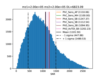
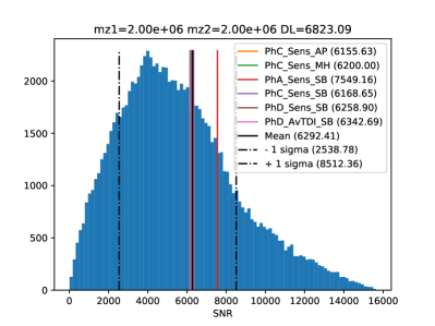
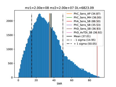
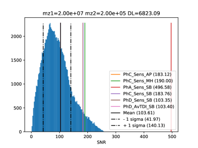
Figure 12: TC1: Numerical results and analytical results for the non-spinning cases and redshift 1. The intrinsic masses of the source are : row 1: $10^{5}-10^{5}$ and $10^{6}-10^{6}$, row 2: $10^{7}-10^{7}$ and $10^{8}-10^{8}$, row 3: $10^{6}-10^{5}$ and $10^{7}-10^{6}$, row 4: $10^{8}-10^{7}$ and $10^{7}-10^{5}$

C.2 Test case 2

Reference system: non-spinning $\chi_{1}=\chi_{2}=0$, redshift $z=8$, luminosity distance $D_{L}=81480.3$ Mpc, source frame individual masses $m_{i}=10^{5},10^{6},10^{7},10^{8}$.

The table 6 is summarizing the results with various methods and the figure 13 is showing a comparison of the results including the distribution of SNRs.

$m_{1}|m_{2}$		$1\times 10^{5}$	$1\times 10^{6}$	$1\times 10^{7}$	$1\times 10^{8}$
$1\times 10^{5}$	PhD Num AP	$298_{-178}^{+105}$	$97_{-58}^{+34}$	$1_{-1}^{+1}$	-
	PhC Sens AP	298	102	2	-
	PhC Sens MH	300	100	2	-
	PhA Sens SB	366	222	7	-
	PhC Sens SB	298	103	2	-
	PhD Sens SB	296	97	1	-
	PhD AvTDI SB	306	97	1	-
$1\times 10^{6}$	PhD Num AP	-	$341_{-203}^{+120}$	$10_{-6}^{+3}$	$0_{-0}^{+0}$
	PhC Sens AP	-	336	9	-
	PhC Sens MH	-	340	10	-
	PhA Sens SB	-	407	22	0
	PhC Sens SB	-	336	9	0
	PhD Sens SB	-	340	10	0
	PhD AvTDI SB	-	340	10	-
$1\times 10^{7}$	PhD Num AP	-	-	$26_{-16}^{+9}$	$0_{-0}^{+0}$
	PhC Sens AP	-	-	26	-
	PhC Sens MH	-	-	26	-
	PhA Sens SB	-	-	31	1
	PhC Sens SB	-	-	26	0
	PhD Sens SB	-	-	26	0
	PhD AvTDI SB	-	-	26	-
$1\times 10^{8}$	PhD Num AP	-	-	-	$1_{-1}^{+0}$
	PhC Sens AP	-	-	-	-
	PhC Sens MH	-	-	-	-
	PhA Sens SB	-	-	-	-
	PhC Sens SB	-	-	-	-
	PhD Sens SB	-	-	-	-
	PhD AvTDI SB	-	-	-	-

Table 6: SNRs for TC2, i.e. $\chi_{1}=\chi_{2}=0$ and redshift 8.

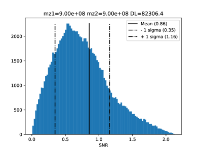
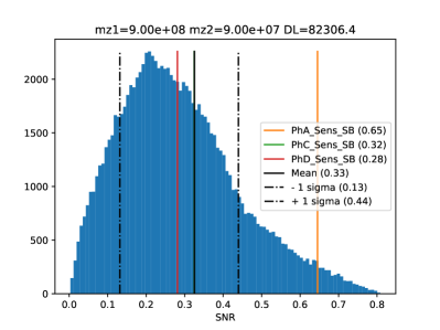
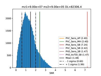
Figure 13: TC2: Numerical results and analytical results for the non-spinning cases and redshift 8. The intrinsic masses of the source are : row 1: $10^{5}-10^{5}$ and $10^{6}-10^{6}$, row 2: $10^{7}-10^{7}$ and $10^{8}-10^{8}$, row 3: $10^{6}-10^{5}$ and $10^{7}-10^{6}$, row 4: $10^{8}-10^{7}$ and $10^{7}-10^{5}$

C.3 Test case 3

Reference system: equal spins $\chi_{1}=\chi_{2}=0.5$, redshift $z=1$, luminosity distance $D_{L}=6823$ Mpc, source frame individual masses $m_{i}=10^{5},10^{6},10^{7},10^{8}$.

The table 7 is summarizing the results with various methods and the figure 14 is showing a comparison of the results including the distribution of SNRs.

$m_{1}|m_{2}$		$1\times 10^{5}$	$1\times 10^{6}$	$1\times 10^{7}$	$1\times 10^{8}$
$1\times 10^{5}$	PhD Num AP	$1174_{-687}^{+404}$	$1851_{-1104}^{+653}$	$205_{-122}^{+72}$	-
	PhC Sens AP	1172	2045	430	-
	PhC Sens SB	1172	2044	431	-
	PhD Sens SB	1168	1842	204	-
	PhD AvTDI SB	1288	1876	205	-
$1\times 10^{6}$	PhD Num AP	-	$7643_{-4558}^{+2697}$	$1135_{-677}^{+400}$	$12_{-7}^{+4}$
	PhC Sens AP	-	7468	1163	27
	PhC Sens SB	-	7466	1164	29
	PhD Sens SB	-	7602	1132	12
	PhD AvTDI SB	-	7721	1133	12
$1\times 10^{7}$	PhD Num AP	-	-	$3169_{-1889}^{+1117}$	$70_{-42}^{+25}$
	PhC Sens AP	-	-	3164	68
	PhC Sens SB	-	-	3165	69
	PhD Sens SB	-	-	3161	70
	PhD AvTDI SB	-	-	3162	70
$1\times 10^{8}$	PhD Num AP	-	-	-	$156_{-93}^{+55}$
	PhC Sens AP	-	-	-	156
	PhC Sens SB	-	-	-	164
	PhD Sens SB	-	-	-	159
	PhD AvTDI SB	-	-	-	156

Table 7: SNRs for TC3, i.e. $\chi_{1}=\chi_{2}=0.5$ and redshift 1.

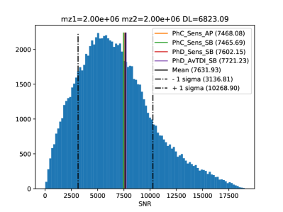
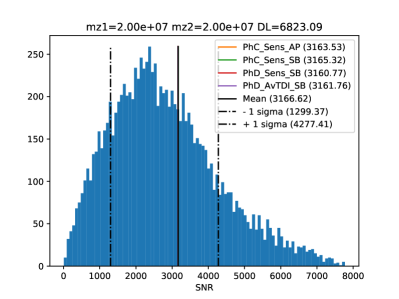
Figure 14: TC3: Numerical results and analytical results for $\chi_{1}=\chi_{2}=0.5$ and redshift 1. The intrinsic masses of the source are : row 1: $10^{5}-10^{5}$ and $10^{6}-10^{6}$, row 2: $10^{7}-10^{7}$ and $10^{8}-10^{8}$, row 3: $10^{6}-10^{5}$ and $10^{7}-10^{6}$, row 4: $10^{8}-10^{7}$ and $10^{7}-10^{5}$

C.4 Test case 4

Reference system: equal spins $\chi_{1}=\chi_{2}=-0.5$, redshift $z=1$, luminosity distance $D_{L}=6823$ Mpc, source frame individual masses $m_{i}=10^{5},10^{6},10^{7},10^{8}$.

The table 8 is summarizing the results with various methods and the figure 15 is showing a comparison of the results including the distribution of SNRs.

$m_{1}|m_{2}$		$1\times 10^{5}$	$1\times 10^{6}$	$1\times 10^{7}$	$1\times 10^{8}$
$1\times 10^{5}$	PhD Num	$1024_{-601}^{+352}$	$1074_{-632}^{+371}$	$68_{-40}^{+23}$	-
	PhD Sens	1020	1070	68	-
	PhD AvTDI	1116	1086	68	-
	PhC Sens	1053	1468	616	-
$1\times 10^{6}$	PhD Num	-	$5370_{-3163}^{+1855}$	$461_{-272}^{+159}$	$3_{-2}^{+1}$
	PhD Sens	-	5349	461	3
	PhD AvTDI	-	5412	461	3
	PhC Sens	-	5231	770	42
$1\times 10^{7}$	PhD Num	-	-	$1590_{-936}^{+549}$	$24_{-14}^{+8}$
	PhD Sens	-	-	1588	24
	PhD AvTDI	-	-	1588	24
	PhC Sens	-	-	1555	45
$1\times 10^{8}$	PhD Num	-	-	-	$70_{-41}^{+24}$
	PhD Sens	-	-	-	71
	PhD AvTDI	-	-	-	70
	PhC Sens	-	-	-	71

Table 8: TC4 SNRs.

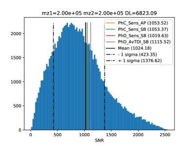
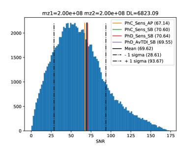
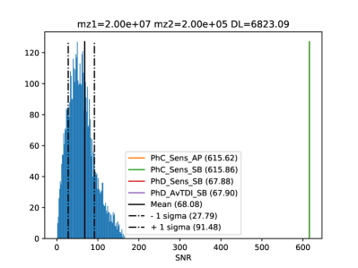
Figure 15: TC4: Numerical results and analytical results for $\chi_{1}=\chi_{2}=0.5$ and redshift 1. The intrinsic masses of the source are : row 1: $10^{5}-10^{5}$ and $10^{6}-10^{6}$, row 2: $10^{7}-10^{7}$ and $10^{8}-10^{8}$, row 3: $10^{6}-10^{5}$ and $10^{7}-10^{6}$, row 4: $10^{8}-10^{7}$ and $10^{7}-10^{5}$

C.5 Test case 5

Reference system: spins $\chi_{1}=0.7,\;\chi_{2}=0.9$, redshift $z=1$, luminosity distance $D_{L}=6823$ Mpc, source frame individual masses $m_{i}=10^{5},10^{6},10^{7},10^{8}$.

The table 9 is summarizing the results with various methods and the figure 16 is showing a comparison of the results including the distribution of SNRs.

$m_{1}|m_{2}$		$1\times 10^{5}$	$1\times 10^{6}$	$1\times 10^{7}$	$1\times 10^{8}$
$1\times 10^{5}$	PhD Num	$1215_{-711}^{+418}$	$2169_{-1277}^{+749}$	$313_{-186}^{+108}$	-
	PhD Sens	1210	2161	312	-
	PhD AvTDI	1342	2207	313	-
	PhC Sens	1209	2383	697	-
$1\times 10^{6}$	PhD Num	-	$8835_{-5205}^{+3051}$	$1569_{-924}^{+542}$	$20_{-12}^{+7}$
	PhD Sens	-	8801	1567	20
	PhD AvTDI	-	8960	1568	20
	PhC Sens	-	8712	1798	54
$1\times 10^{7}$	PhD Num	-	-	$4412_{-2599}^{+1525}$	$105_{-63}^{+37}$
	PhD Sens	-	-	4407	105
	PhD AvTDI	-	-	4409	105
	PhC Sens	-	-	4364	117
$1\times 10^{8}$	PhD Num	-	-	-	$234_{-139}^{+83}$
	PhD Sens	-	-	-	237
	PhD AvTDI	-	-	-	233
	PhC Sens	-	-	-	223

Table 9: TC5 SNRs

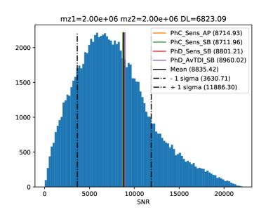
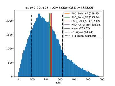
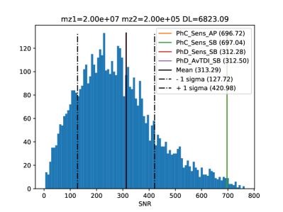
Figure 16: TC4: Numerical results and analytical results for $\chi_{1}=0.7$ and $\chi_{2}=0.9$ and redshift 1. The intrinsic masses of the source are : row 1: $10^{5}-10^{5}$ and $10^{6}-10^{6}$, row 2: $10^{7}-10^{7}$ and $10^{8}-10^{8}$, row 3: $10^{6}-10^{5}$ and $10^{7}-10^{6}$, row 4: $10^{8}-10^{7}$ and $10^{7}-10^{5}$

C.6 IMR model comparison.

We have implemented and used three IMRPhenom models in the evaluation of SNR. We need to be aware os systematics in those models: the models have different fidelity across the parameter space. The comparable mass ratio non-spinning NR waveforms were used to fit IMRPhenomA model, moreover, only leading order SPA amplitude is used at low frequency. IMRPhenomC was calibrated up to mass ratio 4 and uses combination of two spins as a parameter. The most accurate model (among considered) is IMRPhenomD, it uses two spin magnitudes and was calibrated up to mass ratio 16. Use of any of these models outside the corresponding domain of validity might lead to erroneous results.

We have performed the monte-carlo simulation in $m_{1}-m_{2}$ space (uniform in the total mass $\log_{10}(m_{1}+m_{2})\in U[5,9]$, uniform in the mass ratio $q=m1/m2\in U[1,50]$) of non-spinning MBHBs. For each model we have computed the sky, polarization, inclination averaged SNR using three models. In two plots below [17], [18] we give (color-coded) ratios of $SNR_{A}/SNR_{D}$ and $SNR_{C}/SNR_{D}$.

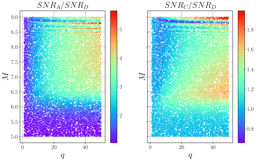
Figure 17: Monte carlo simulation. Computation of SNR ratio for IMR models. Total mass $M=m_{1}+m_{2}$ vs mass ratio $q=m_{1}/m_{2}$, SNR ratio is color-coded.

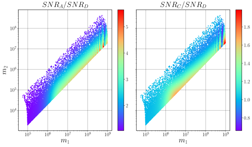
Figure 18: Monte carlo simulation. Computation of SNR ratio for IMR models. Component masses (observed) are given along axes, SNR ratio is color-coded.

Acronyms

References

- [1] Repository for lisa sensitvity and snr on public lisa gitlab. https://gitlab.in2p3.fr/lisa/lisa_sensitivity_snr. https://gitlab.in2p3.fr/lisa/lisa_sensitivity_snr.
- [2] Matthew R. Adams and Neil J. Cornish. Detecting a stochastic gravitational wave background in the presence of a galactic foreground and instrument noise. Phys. Rev. D, 89(2):022001, January 2014.
- [3] P. Ajith, S. Babak, Y. Chen, M. Hewitson, B. Krishnan, A. M. Sintes, J. T. Whelan, B. Brügmann, P. Diener, N. Dorband, J. Gonzalez, M. Hannam, S. Husa, D. Pollney, L. Rezzolla, L. Santamaría, U. Sperhake, and J. Thornburg. Template bank for gravitational waveforms from coalescing binary black holes: Nonspinning binaries. Phys. Rev. D, 77(10):104017, May 2008.
- [4] Jean-Baptiste Bayle. Simulation and Data Analysis for LISA (Instrumental Modeling, Time-Delay Interferometry, Noise-Reduction Performance Study, and Discrimination of Transient Gravitational Signals). Theses, Université de Paris ; Université Paris Diderot ; Laboratoire Astroparticules et Cosmologie, October 2019.
- [5] Jean-Baptiste Bayle, Marc Lilley, Antoine Petiteau, and Hubert Halloin. Effect of filters on the time-delay interferometry residual laser noise for LISA. Phys. Rev. D, 99(8):084023, April 2019.
- [6] Raphael Flauger, Nikolaos Karnesis, Germano Nardini, Mauro Pieroni, Angelo Ricciardone, and Jesús Torrado. Improved reconstruction of a stochastic gravitational wave background with LISA. J. Cosmology Astropart. Phys, 2021(1):059, January 2021.
- [7] David W. Hogg. Distance measures in cosmology. arXiv e-prints, pages astro–ph/9905116, May 1999.
- [8] Sebastian Khan, Sascha Husa, Mark Hannam, Frank Ohme, Michael Pürrer, Xisco Jiménez Forteza, and Alejandro Bohé. Frequency-domain gravitational waves from nonprecessing black-hole binaries. II. A phenomenological model for the advanced detector era. Phys. Rev. D, 93(4):044007, February 2016.
- [9] Valeriya Korol, Elena M. Rossi, Paul J. Groot, Gijs Nelemans, Silvia Toonen, and Anthony G. A. Brown. Prospects for detection of detached double white dwarf binaries with Gaia, LSST and LISA. Mon. Not. Roy. Astron. Soc., 470(2):1894–1910, 2017.
- [10] Shane L. Larson, William A. Hiscock, and Ronald W. Hellings. Sensitivity curves for spaceborne gravitational wave interferometers. Phys. Rev. D, 62(6):062001, September 2000.
- [11] LISA Consortium. LISA Performance Model and Error Budget, LISA-LCST-INST-TN-003. Technical Report 2.0, ESA, 2020.
- [12] LISA Science Study Team. LISA Science Requirements Document, ESA-L3-EST-SCI-RS-001. Technical Report 1.0, ESA, May 2018. https://www.cosmos.esa.int/web/lisa/lisa-documents/.
- [13] M. Otto. Time-Delay Interferometry Simulations for the Laser Interferometer Space Antenna. PhD thesis, Leibniz Universitat Hannover, 2016.
- [14] Antoine Petiteau. DE LA SIMULATION DE LISA A L’ANALYSE DES DONNEES. Détection d’ondes gravitationnelles par interférométrie spatiale (LISA : Laser Interferometer Space Antenna). Theses, Université Paris-Diderot - Paris VII, June 2008.
- [15] Antoine Petiteau, Gerard Auger, Hubert Halloin, Olivier Jeannin, Sophie Pireaux, Eric Plagnol, Tania Regimbau, and Jean-Yves Vinet. LISACode: Simulating Lisa. In Stephen M. Merkovitz and Jeffrey C. Livas, editors, Laser Interferometer Space Antenna: 6th International LISA Symposium, volume 873 of American Institute of Physics Conference Series, pages 633–639, November 2006.
- [16] Planck Collaboration, P. A. R. Ade, N. Aghanim, M. Arnaud, M. Ashdown, J. Aumont, C. Baccigalupi, A. J. Banday, R. B. Barreiro, J. G. Bartlett, and et al. Planck 2015 results. XIII. Cosmological parameters. A&A, 594:A13, September 2016.
- [17] Thomas A. Prince, Massimo Tinto, Shane L. Larson, and J. W. Armstrong. LISA optimal sensitivity. Phys. Rev. D, 66(12):122002, December 2002.
- [18] L. Santamaría, F. Ohme, P. Ajith, B. Brügmann, N. Dorband, M. Hannam, S. Husa, P. Mösta, D. Pollney, C. Reisswig, E. L. Robinson, J. Seiler, and B. Krishnan. Matching post-Newtonian and numerical relativity waveforms: Systematic errors and a new phenomenological model for nonprecessing black hole binaries. Phys. Rev. D, 82(6):064016, September 2010.
- [19] Kip S. Thorne and Roger D. Blandford. Modern Classical Physics Optics, Fluids, Plasmas, Elasticity, Relativity, and Statistical Physics. 2017.
- [20] Eric Thrane and Joseph D. Romano. Sensitivity curves for searches for gravitational-wave backgrounds. Phys. Rev. D, 88(12):124032, December 2013.
- [21] Seth E. Timpano, Louis J. Rubbo, and Neil J. Cornish. Characterizing the galactic gravitational wave background with LISA. Phys. Rev. D, 73(12):122001, June 2006.