Conformal and Uniformizing Maps in Borel Analysis

Abstract

Perturbative expansions in physical applications are generically divergent, and their physical content can be studied using Borel analysis. Given just a finite number of terms of such an expansion, this input data can be analyzed in different ways, leading to vastly different precision for the extrapolation of the expansion parameter away from its original asymptotic regime. Here we describe how conformal maps and uniformizing maps can be used, in conjunction with Padé approximants, to increase the precision of the information that can be extracted from a finite amount of perturbative input data. We also summarize results from the physical interpretation of Padé approximations in terms of electrostatic potential theory.

I Introduction

Perturbation theory is generically divergent, but in principle it contains a wealth of physical information also about non-perturbative effects [1]. However, in difficult problems it is often challenging to compute many orders of a perturbative expansion. This raises the mathematical question of how best to extract as much information as possible from a finite number of terms of an expansion. The first main conclusion is that it is more effective to map the problem to the Borel plane, converting the divergent series to a convergent Borel transform function, dividing out the generic leading factorial growth. This simple step smoothens the problem, enabling the use of a vast array of powerful tools of complex analysis. At a deeper level one can use the full machinery of resurgent asymptotics [2, 3] to probe the system in all parametric regions. The question now becomes: given a finite number of terms of an expansion of a Borel transform function $\mathcal{B}(p)$, what can we learn about its analytic structure in the complex $p$ plane? Singularities of $\mathcal{B}(p)$ have special physical significance, as they are directly related to non-perturbative physics and with associated Stokes phenomena.

Thus we can summarize our motivation as follows: given a finite number of terms in the expansion of a Borel function $\mathcal{B}(p)$ about some point (say, $p=0$), we ask what is the optimal procedure, and what are effective near-optimal approximations to answer the following questions:

1. Where are the singularities $p_{0}$ of $\mathcal{B}(p)$ in the complex $p$ plane? This might refer, for example, to locating a phase transition.

2. What is the nature (exponent $\alpha$) of each singularity? $\mathcal{B}(p)\sim(p-p_{0})^{\alpha}$. This is relevant for determining critical exponents.

3. What is the coefficient of the leading singularity (or leading singularities)? $\mathcal{B}(p)\sim\mathcal{S}(p-p_{0})^{\alpha}$. This relates to the determination of Stokes constants.

4. Can one extrapolate from one Riemann sheet to the next? This is also important for the study of phase transitions.

Many ingenious ad hoc methods have been developed for different mathematical and physical applications. Here we describe recent work aimed at developing a systematic mathematical framework to find optimal methods to solve these problems [4, 5, 6]. We refer to this as “inverse approximation theory”, because the task is to learn as much as possible about some function, based on partial information about it, rather than finding efficient approximations for a given function. For the wide class of resurgent functions, which arise frequently in applications and are expected to suffice for all natural problems, new practical approximation methods can achieve near-optimal results, especially in the vicinity of the singularities.

In this paper we restrict our attention to Borel analysis, but note that there are also interesting applications to certain problems where the physical function of interest is itself convergent, but we wish to learn about its radius of convergence (i.e., its singularities). A simple example is the Ising model, where the free energy has a finite radius of convergence, and we might wish to determine the behavior in the vicinity of the critical temperature by extrapolating from an expansion at either low or high temperature.

The key mathematical tools described here are Borel summation [3], Padé approximants [7], conformal maps and uniformizing maps [8, 9]. These are of course well-studied methods, which have been used empirically in these kinds of investigations [10, 11, 12]. Here we seek to explain how and why these methods work, and to compare their precision in quantifiable ways. The main message is that by combining them in various different ways, we can obtain dramatically improved precision in exploring the motivating questions listed above. In situations where we have physical input, even if it is conjectural and/or approximate, concerning the analytic structure of the function under investigation (for example, unitarity or a dispersion relation or a particular symmetry), this information can be used to advantage, and can also be refined iteratively.

II Physics of Padé Approximation: Electrostatic Potential Theory

Padé approximation is a versatile tool for analytic continuation of a function for which only a finite number of expansion coefficients is known [7, 13]. Here we summarize some important results from the physical interpretation of Padé approximation in terms of electrostatic potential theory [14, 15, 6].

The $[M,N]$ Padé approximant of $B(p)$ at $p=0$ is the unique rational function $P_{M}(p)/Q_{N}(p)$, with $P_{M}$ a polynomial of degree at most $M$, and $Q_{N}$ a polynomial of degree at most $N$, for which

$$B(p)-\frac{P_{M}(p)}{Q_{N}(p)}=\mathcal{O}\left(p^{M+N+1}\right),\ \ \ p\to 0$$ (1)

If we normalize $Q_{N}(0)=1$, the Padé polynomials $P_{M}(p)$ and $Q_{N}(p)$ are also unique, and can be calculated algorithmically from the (truncated) Maclaurin series of $B(p)$.

Comments:

• In many applications, diagonal and near-diagonal Padé approximants are the most useful.

• There is a deep connection between Padé approximants and orthogonal polynomials (and their associated large-order Szegö asymptotics [16, 23]) from the fundamental fact that the Padé polynomials $P_{M}$ and $Q_{N}$ satisfy a three-term recursion relation [7, 13].

• In special cases, the convergence of Padé approximants is uniform on compact sets. This is the case for Riesz-Markov functions (i.e., $B(p)=\int_{a}^{b}d\mu(\zeta)/(\zeta-p)$, with $\mu$ a positive measure). See [17] and references therein. While these occur in certain applications, many functions of interest are not Riesz-Markov. For example, a common situation in applications, discussed in more detail in Section III.2 below, is when $B(p)$ has two complex conjugate singularities. Padé produces curved arcs of poles (see Figure 5) which do not relate to the properties of the function.

• In fact, even for single-valued functions, uniform convergence of some diagonal Padé subsequence to general meromorphic functions (the Baker-Gammel-Wills conjecture [18]) does not hold [19]. Pointwise convergence is prevented by the phenomenon of spurious poles, Froissart doublets [20]: “random” pairs of a pole and a nearby zero, unrelated to the function they approximate. The ultimate source of these spurious poles is the fact that the associated polynomials are orthogonal on complex arcs, without a bona-fide Hilbert space structure [14].

II.1 Potential Theory and Physical Interpretation of Padé Approximants

Electrostatic potential theory provides a remarkable and intuitively useful physical interpretation of the Padé domain of convergence and of the location of Padé poles [14, 15, 6]. For this interpretation, it is useful to invert ($p\to 1/p$) to move the point of analyticity from $p=0$ to $p=\infty$. Being rational approximations, Padé approximants can only converge in some domain $\mathcal{D}$ of single-valuedness of the associated function $B(p)$. Furthermore, in general Padé only converges in a weak sense, namely “in capacity”. This means the following. Take any set $\mathcal{D}^{\prime}$ of single-valuedness of $B(p)$, with boundary $E^{\prime}=\partial\mathcal{D}^{\prime}$. Thinking of $E^{\prime}$ as an electrical conductor we place a unit charge on $E^{\prime}$, and normalize the electrostatic potential $V(x,y)=V(p),p=x+iy$ (always constant along a conductor) by $V(E^{\prime})=0$. Then the electrostatic capacitance of $E^{\prime}$ is cap$(E^{\prime})=1/V(\infty)$.

The fundamental result [14] is that the boundary $E=\partial\mathcal{D}$ of the domain of convergence $\mathcal{D}$ of Padé is obtained by deforming the shape of the conductor $E^{\prime}$ (while keeping the singularity locations fixed) until the logarithmic capacity is minimized. Furthermore, the equilibrium measure $\mu$ on $E$ is the equilibrium density of charges on $E$. For points $p\in\mathcal{D}$, the potential is related to the Green’s function $g_{\mathcal{D}}(p)$ as: $e^{-g_{\mathcal{D}}(p)}=e^{-V(p)}$.

Comments:

• Padé “constructs” the maximal domain $\mathcal{D}$ of single-valuedness in which they converge. The rate of convergence near the point of expansion is given by the inverse of the (minimal) capacity and, in a precise sense, it is provably optimal in the class of rational approximations [6].

• Padé represents actual poles of $B(p)$ by poles, and branch points by lines (either straight or curved arcs) of poles accumulating to the branch point. If $B(p)$ has only isolated singularities on the universal cover of $\hat{\mathbb{C}}$ with finitely many punctures, then the boundary of single-valuedness, $\partial\mathcal{D}$, is a set of piecewise analytic arcs joining the branch points of $B(p)$, and some accessory points associated with junctions of these analytic arcs. See for example Figures 5 and 10. The pole density converges in capacity to the equilibrium measure along the arcs, and this density is infinite at the actual branch points, resulting in an accumulation of poles there.

• If $\mathcal{D}$ is simply connected, then $|e^{-g_{\mathcal{D}}}|=|\psi_{\infty}|$, where $\psi_{\infty}$ is a conformal map from $\mathcal{D}$ to the interior of the unit disk, normalized with $\psi_{\infty}(\infty)=0$. Thus Padé effectively “creates its own conformal map” of a single-valuedness domain for $B(p)$. This map can be extracted in the $N\to\infty$ limit from the harmonic function $|e^{-g_{\mathcal{D}}}|$, obtained by taking the $N$-th root of the convergence rate.

• However, this highlights an inherent drawback of the Padé construction: points of interest of $B(p)$ may be hidden on the boundary of convergence. For example, true Borel singularities of $B(p)$ may be obscured by the lines of Padé poles of the minimal capacitor. Nevertheless, the physical intuition behind this potential theory interpretation of Padé approximation enables several simple methods to reveal such “hidden” singularities using conformal maps or probe singularities. See for example the discussion in Section III.3 below, and Figures 9 and 10.

III Borel Transform Functions With Branch Points

The generic singularity of a Borel transform in physical applications is a branch point. Often there is a dominant Borel singularity, associated with the leading divergence of the associated asymptotic series. Cases with multiple Borel singularities are discussed below in Sections III.2 and III.3, in which case there can be interesting interference effects leading to a richer structure of divergent series.

III.1 One Branch Point Borel Singularity

In many physical applications we encounter a formal asymptotic series

$$f(x)\sim\sum_{n=0}^{\infty}\frac{c_{n}}{x^{n+1}}\qquad,\quad x\to+\infty$$ (2)

where the leading rate of growth of the coefficients $c_{n}$ has the “power times factorial” form [1]

$$c_{n}\sim A^{n}\,\Gamma(B\,n+C)\qquad,\quad n\to+\infty$$ (3)

Here the parameters $A$, $B$ and $C$ are constants. In treating such a problem, a natural approach is to apply Borel summation, leading to a Borel-Laplace integral representation of a function $f(x)$ with the asymptotic series (2):

$$f(x)=\int_{0}^{\infty}dp\,e^{-p\,x}\mathcal{B}(p)$$ (4)

This maps the problem of extrapolating $f(x)$ into the complex $x$ plane to the problem of understanding the analytic structure of the Borel transform $\mathcal{B}(p)$, particularly its singularities in the complex Borel $p$ plane.

For example, the following function (based on the incomplete gamma function)

$$F(x;\alpha)\equiv x^{-1-\alpha}\,e^{x}\,\Gamma(1+\alpha,x)=\int_{0}^{\infty}dp\,e^{-p\,x}(1+p)^{\alpha}$$ (5)

has an asymptotic expansion as $x\to+\infty$ of the form in (2)-(3):

$$F(x;\alpha)\sim\frac{1}{\Gamma(-\alpha)}\sum_{n=0}^{\infty}(-1)^{n}\frac{\Gamma(n-\alpha)}{x^{n+1}}\qquad,\quad x\to+\infty$$ (6)

$F(x;\alpha)$ has non-trivial analytic continuation properties in the complex $x$ plane which are encoded in the analytic structure of the Borel transform function $\mathcal{B}(p)=(1+p)^{\alpha}$.

Another example is the function

$$F(x;a,b,c)\equiv\int_{0}^{\infty}dp\,e^{-p\,x}~{}_{2}F_{1}(a,b,c;-p)$$ (7)

which has an asymptotic expansion as $x\to+\infty$

$$F(x;a,b,c)\sim\frac{\Gamma(c)}{\Gamma(a)\,\Gamma(b)}\sum_{n=0}^{\infty}(-1)^{n}\frac{\Gamma(n+a)\,\Gamma(n+b)}{\Gamma(n+c)}\frac{1}{x^{n+1}}\qquad,\quad x\to+\infty$$ (8)

The expansion coefficients have leading large order growth as in (3), but now with further subleading power-law corrections:

$$c_{n}\sim\frac{\Gamma(c)}{\Gamma(a)\,\Gamma(b)}\,(-1)^{n}\,\Gamma(n+a+b-c)\left[1-\frac{(a-c)(b-c)}{n}+O\left(\frac{1}{n^{2}}\right)\right]$$ (9)

The Borel transform functions in (5) and (7), $\mathcal{B}(p)=(1+p)^{\alpha}$ and $\mathcal{B}(p)=~{}_{2}F_{1}(a,b,c;-p)$, respectively, have the common feature of possessing just one branch point, which we have normalized here to lie at $p=-1$.

In the physically relevant situation in which we only know a finite number of coefficients $c_{n}$ of the asymptotic expansion (2), there are several different approaches to analyze the singularity structure of the associated Borel transform. Padé approximants are a key tool in analytically continuing the truncated Borel transform beyond its radius of convergence, but they can be significantly improved by combining them with conformal and uniformizing maps.

Padé-Borel transform: Padé approximants provide remarkably accurate extrapolations and analytic continuations of truncated expansions [7, 13]. For a truncation of an asymptotic series it is generally better to apply a Padé approximation in the Borel $p$ plane than in the original $x$ plane. Thus, we apply Padé to the convergent Borel transform function rather than to the divergent large $x$ expansion (2). This procedure is referred to as Padé-Borel ($\mathcal{PB}$). Note that Padé is a non-linear operation, so it does not commute with the linear Borel transform (4). The higher precision of Padé-Borel has been observed empirically and it is widely used [21, 10, 22]. The improved precision has recently been proven with explicit error bounds for the canonical example (5) [5], for which the exact $[N,N]$ diagonal Padé-Borel transform is

$${\rm Pade}{\rm-}{\rm Borel:}\qquad{\mathcal{PB}}_{[N,N]}(p;\alpha)=\frac{P_{N}^{(\alpha,-\alpha)}\left(1+\frac{2}{p}\right)}{P_{N}^{(-\alpha,\alpha)}\left(1+\frac{2}{p}\right)}$$ (10)

Here $P_{N}^{(\alpha,\beta)}$ is the $N^{\rm th}$ Jacobi polynomial. The large $N$ asymptotics of the Jacobi polynomials explains why $\mathcal{PB}$ yields such an improvement.

Padé-Conformal-Borel transform: if there is a dominant Borel branch point singularity, an even more accurate summation than $\mathcal{PB}$ is obtained by first making a conformal map from the cut Borel plane $p\in{\mathbb{C}}\setminus(-\infty,-1]$ to the interior of the unit disc $|z|<1$ using the conformal map:

$$p=\frac{4z}{(1-z)^{2}}\quad\longleftrightarrow\quad z=\frac{\sqrt{1+p}-1}{\sqrt{1+p}+1}$$ (11)

and then making a Padé approximant in the $z$ plane. This conformal map takes the singularity at $p=-1$ to $z=-1$, and $p=0$ to $z=0$, while $z=1$ corresponds to the point at infinity in the $p$ plane. The upper/lower edge of the cut $p\in(-\infty,-1]$ maps to upper/lower unit circle in the $z$ plane. For example, the points $p=-2\pm i\epsilon$ (as $\epsilon\to 0^{+}$) map to $z=\pm i$. Conformal maps are frequently used in series analysis [12, 11, 10], and when combined with a subsequent Padé approximant, there is a significant further gain in precision [5]. For example, the $\mathcal{PB}$ result (10) is replaced by the closed-form Padé-Conformal-Borel ($\mathcal{PCB}$) transform:

$${\rm Pade}{\rm-}{\rm Conformal}{\rm-}{\rm Borel:}\qquad{\mathcal{PCB}}_{[N,N]}(p;\alpha)=\frac{P_{N}^{(2\alpha,-2\alpha)}\left(\frac{\sqrt{1+p}+1}{\sqrt{1+p}-1}\right)}{P_{N}^{(-2\alpha,2\alpha)}\left(\frac{\sqrt{1+p}+1}{\sqrt{1+p}-1}\right)}$$ (12)

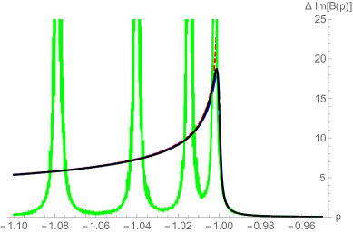
Figure 1: Plot of the jump in the imaginary part of the hypergeometric Borel function $B(p)=~{}_{2}F_{1}\left(\frac{2}{3},\frac{2}{3},1;-p\right)$, across the cut $p\in(-\infty,-1]$, based on just $10$ terms of a truncated asymptotic expansion. The blue and black curves are the jump for $p\pm 10^{-3}i$, just above and below the cut, for the exact function and its $\mathcal{PCB}$ and $\mathcal{PUB}$ approximations. These three curves are indistinguishable on this scale. The red dashed curve is the exact jump using properties of hypergeometric functions, while the green curve is the jump in the Padé-Borel approximation. We see the effect of the Padé poles along the cut. The jittery nature of the Padé-Borel approximation can be improved by converting the Padé polynomial ratio to a partial fraction expansion.

Comments:

• We stress that the $\mathcal{PCB}$ result (12) is obtained from exactly the same input information ($2N$ terms of the truncated asymptotic series) as the $\mathcal{PB}$ result (10), but is significantly more accurate.

• This increased precision is particularly dramatic near the Borel cut. See Figure 1. The Padé-Borel transform (10) places unphysical poles along the negative $p$ axis, $p\in(-\infty,-1]$, accumulating to the branch point at $p=-1$, in an attempt to use rational functions to approximate the natural branch cut of the exact Borel transform function [7, 14, 15, 23, 6]. On the other hand, the Padé-Conformal-Borel transform (12) has no unphysical poles along the negative $p$ axis, and hence represents the behavior near the Borel branch point and branch cut much more precisely, as is quantified in [5] using the large $N$ asymptotics of the relevant Jacobi polynomials.

• The conformal map (11) does not require knowledge of the nature of the branch point, only its location (which we have re-scaled here to lie at $p=-1$). Correspondingly, the leading large $N$ asymptotics of the Padé polynomials is independent of the exponent $\alpha$. However, square root branch points ($\alpha=\pm\frac{1}{2}$) are special, as in this case the Padé-Conformal-Borel transform is exact for all $N$. The conformal map converts a square root branch point to a pole. See Figure 2. This extreme sensitivity leads to the singularity elimination method [6], which can be applied iteratively to obtain remarkably precise knowledge of the exact location and exponent of a Borel singularity.

• In practical computations, it is often more stable numerically to convert the Padé approximant in the $z$ plane to a partial fraction expansion, and then map back to the Borel $p$ plane.

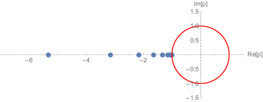
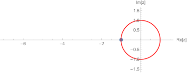
Figure 2: The first plot shows the Padé poles for the $\mathcal{PB}$ approximation to the Borel function $\mathcal{B}(p)=(1+p)^{-1/2}$, from 20 terms of the small $p$ expansion. The square root branch cut is represented approximately as a line of Padé poles accumulating to the branch point at $p=-1$. The second plot shows the Padé poles in the conformally mapped $z$ plane, with the same input, but after the conformal map in (11). The branch point is mapped to a pole, and Padé is in fact exact.

Padé-Uniformized-Borel transform: if there is a dominant Borel branch point singularity, an even more accurate analytic continuation of the truncated Borel transform function (and hence a more accurate summation of the associated asymptotic series) is obtained by using the uniformizing map of the cut plane:

$$p=-1+e^{s}\quad\longleftrightarrow\quad s=\log(1+p)$$ (13)

This uniformizing map $p=-1+e^{s}$ is a $1$-$1$ map between the complex plane and the infinite sheeted Riemann surface of the logarithm function $\log(1+p)$ on ${\mathbb{C}}$ with the singular point at $p=-1$ removed [24, 25, 6]. The point $p=-1$ (the singularity of the logarithm) is a boundary point of this Riemann surface, and is mapped into the boundary point at infinity of the complex $s$ plane (the singularity of the exponential function).

For the incomplete gamma function example (5), the exact diagonal Padé approximant is

$${\rm Pade}{\rm-}{\rm Uniformized}{\rm-}{\rm Borel:}\quad{\mathcal{PUB}}_{[N,N]}(p;\alpha)=\frac{~{}_{1}F_{1}(-N,-2N;\alpha\log(1+p))}{~{}_{1}F_{1}(-N,-2N;-\alpha\log(1+p))}$$ (14)

Once again, large $N$ asymptotics shows that this Padé-Uniformized-Borel ($\mathcal{PUB}$) transform is more precise than either the Padé-Borel or Padé-Conformal-Borel transform. The improvement in precision is especially dramatic in the vicinity of the Borel singularity: see Figure 3.

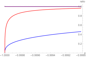
Figure 3: Ratio of $[5,5]$ approximants to the exact Borel transform function $\mathcal{B}(p)=(1+p)^{-1/3}$, as $p\to-1^{+}$. Blue=Padé-Borel; Red=Padé-Conformal-Borel; Purple= Padé-Uniformizing-Borel. Note the extreme precision of the $\mathcal{PUB}$ approximation compared to the other approximations, especially in the vicinity of the singularity at $p=-1$. Note that each approximation was generated with the same input data: just 10 terms of the truncated expansion.

Comments:

• The improvement due to the uniformizing map is particularly dramatic near the singularity. See Figure 3.

• This uniformizing map approach to analytically continuing the truncated Borel transform function is in fact the optimal extrapolation, in the sense that this extrapolation constructs the best approximant (i.e., with minimized errors) within the class of all functions analytic on a common Riemann surface (and with common bounds). For details see [6].

• Analogous results are straightforwardly obtained for a Borel transform with a logarithmic branch cut, $\mathcal{B}(p)=\ln(1+p)$, by taking derivatives with respect to the exponent $\alpha$.

• While analytic results for the precision were obtained in [5] for the asymptotic series having the generic leading large order factorial growth, the incomplete gamma function example in (5), the results apply more generally [4, 6]. For example, the hypergeometric Borel transform function in (7) has the same hierarchy of the quality of representations. See for example Figure 1.

• Recall that more precise analytic knowledge of the Borel transform $\mathcal{B}(p)$ yields more precise analytic knowledge of the physical function $f(x)$ in (4). In fact, the improved analytic continuation of $\mathcal{B}(p)$ from the $\mathcal{PUB}$ approximation also permits analytic continuation onto higher Riemann sheets, which is not possible with the other methods [6].

• The uniformization method applies in principle to functions with any number of branch points.

III.2 Two Borel Singularities

In applications there often exist two Borel singularities (or two dominant Borel singularities). In this case there are also explicit conformal maps and uniformizing maps which improve significantly the precision of the analytic continuation of the Borel transform.

III.2.1 Two Symmetric Collinear Borel Singularities

Suppose we have two symmetric singularities in the Borel plane, scaled to be at $p=\pm 1$. A simple example is the Borel transform function:

$$B(p;\alpha)=\left(1-p^{2}\right)^{\alpha}$$ (15)

In this case, the conformal map in (11) generalizes to

$$p=\frac{2z}{(1+z^{2})}\quad\longleftrightarrow\quad z=\sqrt{\frac{1-\sqrt{1-p^{2}}}{1+\sqrt{1-p^{2}}}}$$ (16)

The $\mathcal{PB}$ and $\mathcal{PCB}$ approximations generalize in a straightforward way [compare with (10) and (12)]:

$${\rm Pade}{\rm-}{\rm Borel:}\qquad{\mathcal{PB}}_{[N,N]}(p;\alpha)=\frac{P_{N}^{(\alpha,-\alpha)}\left(1-\frac{2}{p^{2}}\right)}{P_{N}^{(-\alpha,\alpha)}\left(1-\frac{2}{p^{2}}\right)}$$ (17)

$${\rm Pade}{\rm-}{\rm Conformal}{\rm-}{\rm Borel:}\qquad{\mathcal{PCB}}_{[N,N]}(p;\alpha)=\frac{P_{N}^{(2\alpha,-2\alpha)}\left(\frac{\sqrt{1-p^{2}}+1}{\sqrt{1-p^{2}}-1}\right)}{P_{N}^{(-2\alpha,2\alpha)}\left(\frac{\sqrt{1-p^{2}}+1}{\sqrt{1-p^{2}}-1}\right)}$$ (18)

The $\mathcal{PUB}$ approximation uses the uniformizing map for the universal covering of $\hat{\mathbb{C}}\setminus\{-1,1,\infty\}$:

$$p=-1+2\lambda\left(i\,\frac{1-z}{1+z}\right)\quad\longleftrightarrow\quad z=\frac{{\mathbb{K}}\left(\frac{1+p}{2}\right)-{\mathbb{K}}\left(\frac{1-p}{2}\right)}{{\mathbb{K}}\left(\frac{1-p}{2}\right)+{\mathbb{K}}\left(\frac{1+p}{2}\right)}$$ (19)

Here $\lambda=\theta_{2}^{4}/\theta_{3}^{4}$ is the elliptic modular function, $\theta_{2},\theta_{3}$ are Jacobi theta functions, and ${\mathbb{K}}(m)=(\pi/2)\,_{2}F_{1}(\frac{1}{2},\frac{1}{2};1;m)$ is the complete elliptic integral of the first kind of modulus $m=k^{2}$ [8]. As before, the $\mathcal{PUB}$ approximation involves mapping from the Borel $p$ plane to the $z$ plane, making a Padé approximant in $z$, and then mapping back to the Borel $p$ plane using the inverse map. The $\mathcal{PB}$ approximation places unphysical poles along the two cuts, while the $\mathcal{PCB}$ and $\mathcal{PUB}$ approximation provide a very accurate representation of the Borel cuts, even using just 20 terms of the original asymptotic expansion. See Figure 4.

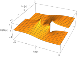
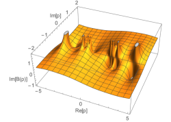
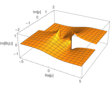
Figure 4: Plots of the imaginary part of the Borel function $\mathcal{B}(p)=(1-p^{2})^{-1/3}$ for (i) the exact function; (ii) [10,10] diagonal Padé-Borel approximant; (iii) [10,10] diagonal Padé-Conformal-Borel approximant; (iv) [10,10] diagonal Padé-Uniformized-Borel approximant. In (ii) Padé places unphysical poles along the branch cuts, while the $\mathcal{PCB}$ and $\mathcal{PUB}$ approximations are much more accurate in the vicinity of the branch cuts.

Comment:

• The improvement in accuracy with the $\mathcal{PUB}$ approximation is particularly dramatic near the singular points. Indeed, the leading order asymptotic behavior of $z$ near $p=1$ is $z\sim 1+2\pi/\ln(1-p)$. Therefore, in the vicinity of one of the singularities there is exponential “stretching”, $p\sim 1-\exp\left[-\frac{2\pi}{1-z}\right]$, which means for example that $z\approx 0.9$ corresponds to $p\approx 1-5\cdot 10^{-28}$. This enables ultra-precise probing of the $p$ plane singularities.

III.2.2 Two Asymmetric Collinear Borel Singularities

Another common physical configuration of Borel singularities consists of an asymmetric collinear pair of Borel singularities, for example at $p=-a$ and $p=+b$, with $a$ and $b$ both real, with natural cuts $p\in[b,\infty)$ and $p\in(-\infty,-a]$ on either side of the real axis. The corresponding conformal map is:

$$p=\frac{4\,a\,b\,z}{a(1+z)^{2}+b(1-z)^{2}}\quad\longleftrightarrow\quad z=\frac{1-\sqrt{\frac{a(b-p)}{b(a+p)}}}{1+\sqrt{\frac{a(b-p)}{b(a+p)}}}$$ (20)

III.2.3 Complex Conjugate Pair of Borel Singularities

An important physically relevant configuration of two Borel singularities is a complex conjugate pair, which occurs for example in problems with symmetry breaking [26, 27, 28, 29]. We can normalize these to lie at $p=e^{\pm i\theta}$, and choose $\theta\in\left[0,\frac{\pi}{2}\right]$.

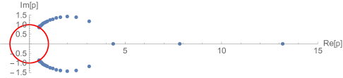
Figure 5: The poles of the Padé approximation to the Borel transform function $\mathcal{B}(p)=(1-2\cos\left(\frac{\pi}{3}\right)p+p^{2})^{-1/3}$, which has a complex conjugate pair of Borel singularities at $p=e^{\pm i\pi/3}$. The unit circle is shown in red. Padé produces arcs of poles emanating from $p=e^{\pm i\pi/3}$, joining and continuing along the positive real $p$ axis. These Padé poles are not related to singularities of the original function $\mathcal{B}(p)$, and limit the precision of the Borel-Laplace integral in (4).

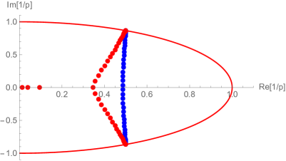
Figure 6: The inverse of the Padé poles for the function $\mathcal{B}(p)=(1-2\cos\left(\frac{\pi}{3}\right)p+p^{2})^{-1/2}$ in blue. These inverse poles show the form of the “minimal capacitor” discussed in Section II. In the limit of infinite Padé order these form a vertical straight line between the two singularities at $p=e^{\pm i\pi/3}$. If the exponent is shifted by a tiny amount, here just $10^{-4}$, the inverse Padé poles (red dots) form a trivalent graph connecting the origin and the two singularities.

Comments:

• The $\mathcal{PB}$ approximation produces two curved arcs of poles, joining to a line of poles along the positive $p$ axis. This illustrates the potential theory interpretation of Padé described in Section II.1. These unphysical poles limit the precision of the Borel-Laplace integral (4). See Figure 5.

• Padé is extremely sensitive to a square root branch point. See Figure 6, which shows that a tiny shift in the exponent away from a square root ($\frac{1}{2}\to\frac{1}{2}-10^{-4}$) has a dramatic and easily recognizable effect on the Padé pole distribution.

For this configuration of two Borel singularities at $p=e^{\pm i\theta}$, the conformal map is

$$p=c(\theta)\frac{z}{(1+z)^{2}}\left(\frac{1+z}{1-z}\right)^{2\theta/\pi}\quad,\quad c(\theta)=4\left(\frac{\theta}{\pi}\right)^{\theta/\pi}\left(1-\frac{\theta}{\pi}\right)^{1-\theta/\pi}$$ (21)

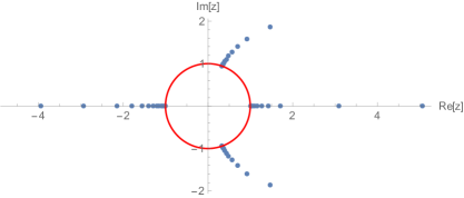
Figure 7: The $z$ plane poles of the Padé approximation to the Borel transform function $\mathcal{B}(p)=(1-2\cos\left(\frac{\pi}{3}\right)p+p^{2})^{-1/3}$, after conformal mapping to the $z$ plane. The unit circle is shown in red. Padé produces arcs of poles emanating from $z=\frac{1}{3}(1\pm 2\sqrt{2}i)$, the conformal map images of $p=e^{\pm i\pi/3}$. The poles accumulating to $z=\pm 1$ correspond to the singularity at $p=\infty$.

Comments:

• With the conformal map (21), the $\mathcal{PCB}$ approximation leads to two symmetric arcs of poles in the conformal $z$ plane, emanating from the conformal map images of $p=e^{\pm i\theta}$. See Figure 7. Note that there is now no obstacle to computing the Borel-Laplace integral in the $z$ plane, integrating from $z=0$ to $z=1$.

• The conformal map (21) is explicit, but its inverse is not, except for special simple rational values of $\theta/\pi$.

For this configuration of two Borel singularities at $p=e^{\pm i\theta}$, the uniformizing map is

$$p=e^{i\,\theta}-2i\,\sin(\theta)\,\lambda\left(i\left(\frac{{\mathbb{K}}\left(\frac{1}{2}+\frac{i}{2}\cot\theta\right)-{\mathbb{K}}\left(\frac{1}{2}-\frac{i}{2}\cot\theta\right)z}{{\mathbb{K}}\left(\frac{1}{2}-\frac{i}{2}\cot\theta\right)+{\mathbb{K}}\left(\frac{1}{2}+\frac{i}{2}\cot\theta\right)z}\right)\right)$$ (22)

where $\lambda$ is the modular $\lambda$ function [8]. The inverse map is explicit:

$$z=\frac{Z(p;\theta)-Z(0;\theta)}{1-\left(Z(0;\theta)\right)^{*}\,Z(p;\theta)}$$ (23)

where $Z(p;\theta)$ is defined as

$$Z(p;\theta)\equiv\frac{{\mathbb{K}}\left(\frac{1}{2}+\frac{i}{2}\left(\frac{p}{\sin\theta}-\cot\theta\right)\right)-{\mathbb{K}}\left(\frac{1}{2}-\frac{i}{2}\left(\frac{p}{\sin\theta}-\cot\theta\right)\right)}{{\mathbb{K}}\left(\frac{1}{2}+\frac{i}{2}\left(\frac{p}{\sin\theta}-\cot\theta\right)\right)+{\mathbb{K}}\left(\frac{1}{2}-\frac{i}{2}\left(\frac{p}{\sin\theta}-\cot\theta\right)\right)}$$ (24)

Comments:

• This uniformizing map and its inverse are both explicit, and it is also significantly more precise than the conformal map (21), especially near the singularities.

• It is straightforward to generalize the uniformizing map of the previous examples to the case of two non-symmetric complex Borel singularities, $p_{1},p_{2}\in{\mathbb{C}}$, using a suitable Möbius transformation and disk automorphism to obtain the universal covering of $\hat{\mathbb{C}}\setminus\{p_{1},p_{2},\infty\}$. The uniformization maps are again expressed in terms of the elliptic function ${\mathbb{K}}$ and the elliptic modular function $\lambda$.

III.3 Three or More Borel Singularities

III.3.1 $k$-fold Symmetrically Distributed Borel Singularities

The general problem of constructing conformal and uniformizing maps with more singularities is a non-trivial problem, even numerically [8, 9, 30, 31, 32]. However, in physical applications the Borel singularities are often distributed symmetrically, in which case more can be done. For example, consider a symmetric $k$-fold set of singularities emanating from the vertices of a regular polygon, such as for the Borel transform function:

$$\mathcal{B}(p;\alpha,k)=\left(1+p^{k}\right)^{\alpha}$$ (25)

The conformal map (11) generalizes to

$$p=\frac{2^{2/k}z}{(1-z^{k})^{2/k}}\quad\longleftrightarrow\quad z^{k}=\frac{\sqrt{1+p^{k}}-1}{\sqrt{1+p^{k}}+1}$$ (26)

with natural branch choices. The $\mathcal{PB}$ and $\mathcal{PCB}$ approximations generalize in a straightforward way, with $p$ simply replaced by $p^{k}$ in the expressions (10) and (12). See Figure 8.

 

 

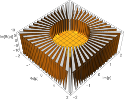
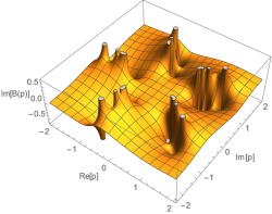
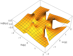
Figure 8: Plots of the imaginary part of the Borel function $\mathcal{B}(p)=(1+p^{5})^{-1/3}$, which has 5 symmetric branch points at $p=e^{(2n+1)i\pi/5}$, for $n=0,1,2,3,4$. The first plot is for the exact function, showing five symmetric radial cuts; the second plot is for 10 terms of the truncated series; the third plot is the Padé-Borel approximation of the 10-term truncated series; the fourth plot is the Padé-Conformal-Borel approximation of the 10-term truncated series. The truncated series is useless beyond $|p|<1$. The $\mathcal{PB}$ approximation extrapolates well away from the cuts, but places unphysical poles along the cuts, while the $\mathcal{PCB}$ approximation is very accurate also near the cuts, starting with just 10 terms.

Comments:

• There is a more general principle underlying this construction. Suppose $p(z)$ is a conformal map of a cut region $\mathcal{D}\in\hat{\mathbb{C}}$ into the unit disk, with $p^{\prime}(z=0)>0$. Then the map $p_{k}(z)=\left(p(z^{k})\right)^{1/k}$ is the conformal map for $k$ symmetric copies of $\mathcal{D}^{1/k}$ [6].

• The same result applies to uniformizing maps.

III.3.2 Schwarz-Christoffel Construction

For more general configurations of singularities, Schwarz-Christoffel provides a constructive approach [9]. For this discussion it is simpler to invert ($p\to 1/p$) to move the point of analyticity from $p=0$ to $p=\infty$. This choice is motivated physically by the electrostatic potential interpretation of Padé approximants [14, 15, 6], in which the potential at infinity is taken to vanish. Then for a general finite set of branch points, $S=\{p_{1},...,p_{n}\}$, Padé produces a conformal map (in the infinite Padé order limit) which corresponds to the minimal capacitor [14, 15, 6]. The expansion at infinity can be written

$$\mathcal{B}(p)=C_{B}p+\sum_{k=0}^{\infty}b_{k}p^{-k}$$ (27)

where $C_{B}$ is the capacity. Using potential theory, there exists a set $\{a_{1},...,a_{n-2}\}$ of (complex) auxiliary parameters such that $\mathcal{B}(p)$ satisfies

$$\log p=\int^{\mathcal{B}(p)}\sqrt{\frac{\prod_{j=1}^{n-2}(s-a_{j})}{\prod_{j=1}^{n}(s-p_{j})}}ds$$ (28)

Geometrically, the auxiliary parameters are the intersection points of the set of analytic arcs of poles of the diagonal Padé approximation for any function $F$ having $S$ as the set of branch points, and being analytic in the complement of the minimal capacitor. See for example the red dots in Figure 10, which have accumulation points at $p=-1$, $p=-2$ and $p=-\frac{3}{2}+\frac{i}{2}$, corresponding to the singularities at these points, and also have two trivalent vertices near $p=-2+\frac{3i}{20}$ and $p=-\frac{3}{2}+\frac{3i}{10}$. The inverses of these trivalent vertices are the the auxiliary parameters in this case. The analytic arcs $\gamma_{j}$ ($\gamma^{\prime}_{j}$, resp) joining $a_{1}$ with $p_{j},j=1,...,n-1$ ($a_{1}$ to $a_{j},j=2,...,n-2$, resp.) are given by the reality conditions:

$${\rm Re}\left[\int_{\gamma_{k}}^{p}\sqrt{\frac{\prod_{j=1}^{n-2}(s-a_{j})}{\prod_{j=1}^{n}(s-p_{j})}}ds\right]=0\quad\&\quad{\rm Re}\left[\int_{\gamma^{\prime}_{m}}^{p}\sqrt{\frac{\prod_{j=1}^{n-2}(s-a_{j})}{\prod_{j=1}^{n}(s-p_{j})}}ds\right]=0$$ (29)

where $k=1,...,n-1$ and $m=2,...,n-2$. In cases of symmetrically distributed branch points, these integrals can be expressed in terms of elementary or elliptic functions [33], and in more general cases the minimal capacitor produced by Padé can be found numerically [34, 32, 35].

III.3.3 Repeated Borel Singularities

For nonlinear problems, such as nonlinear ODEs and PDEs, a given Borel singularity is typically repeated an infinite number of times, often in integer multiples along a ray from the origin. For example, the Borel plane singularities of solutions to nonlinear ODEs, such as the Painlevé equations, lie in integer multiples along the real Borel axis, and this can be uniformized using elliptic functions [6]. In other cases the Borel singularities are repeated in $({\rm integer})^{2}$ multiples [36], or in parabolic arrays [37].

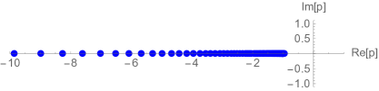
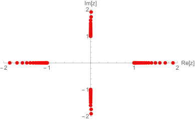
Figure 9: The upper figure shows the Padé poles (blue) of the Borel function $B(p)$ in (30), indicating a branch point at $p=-1$. The singularity at $p=-2$ is obscured by the Padé poles representing the branch cut $p\in(-\infty,-1]$. After the conformal map (11) based on the leading singularity at $p=-1$, the Padé poles in the $z$ plane (red) indicate singularities at $z=\pm 1$ (which are the conformal map images of $p=-1$ and $p=\infty$), and also at $z=\pm i$ (which are the images of $p=-2$ on both sides of the cut).

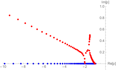
Figure 10: Padé poles (blue) of the Borel function $B(p)$ in (30), indicating a branch point at $p=-1$, and the Padé poles of the Borel function with the addition of the “probe singularity term” in the text. The Padé pole distribution is distorted but the genuine branch point singularity at $p=-2$ can now be seen, in addition to the probe singularity at $p=-\frac{3}{2}+\frac{i}{2}$.

Comments:

• A common problem of the Padé-Borel approximation is that repeated Borel singularities may be hidden by the (unphysical) poles that Padé generates to represent the branch cut associated with the leading singularity. The conformal map of the $\mathcal{PCB}$ approximation resolves this problem by separating the repeated singularities, as separated accumulation points on the unit circle in the conformally mapped $z$ plane [4, 6]. For example, consider the Borel function

  $$B(p)=(1+p)^{-1/3}+\log(2+p)$$ (30)

  for which the poles of a diagonal Padé approximant are shown as blue dots in the first plot of Figure 9. We clearly see the algebraic branch point at $p=-1$, but the logarithmic branch point at $p=-2$ is obscured by the Padé poles attempting to represent the leading cut $p\in(-\infty,-1]$. However, after a conformal map (11) based on the leading singularity, we see that the second singularity at $p=-2$ is cleanly separated and identified, as the conformal map images $z=\pm i$. See the second plot in Figure 9.

• Another simple method [6] to detect repeated singularities that are hidden by unphysical Padé poles is based on the potential theory interpretation of Padé poles as a configuration of charges that distribute themselves in such a way as to minimize the capacitance (relative to infinity) of the arcs along which Padé places its poles (see Section II.1 and [14, 15]). This means that we can introduce another “test charge” by adding to our truncated Borel transform function a singularity near the line of unphysical Padé poles, near where we suspect a true singularity might be hidden. In a subsequent Padé approximation the “minimal capacitor” will be distorted, but the genuine physical singularities do not move. For example, for the Borel function in (30), we can add $B_{\rm probe}=(3/2-i/2+p)^{-1/7}$, which has a new singularity at $p=-\frac{3}{2}+\frac{i}{2}$. Then the Padé pole distribution is distorted to the red dots in Figure 10. The second branch point at $p=-2$ is now clearly visible.

IV Conclusions

It is in general a challenging problem to extract physical information from a limited amount of perturbative information, which is often in the form of a finite number of terms of an expansion which is expected to be asymptotic. However, there are ways to combine Borel summation methods with suitable conformal and uniformizing maps in order to improve and optimize this process. Padé approximants, and their physical interpretation in terms electrostatic potential theory, are particularly useful tools in this analysis. The technical challenge is to probe the singularity structure of the complex Borel plane, starting with only a finite number of coefficients in the expansion of the Borel transform, combined possibly with some information about the expected global structure of the underlying Riemann surface. For realistic model examples, with the typical physical “factorial times power” rate of growth of coefficients (3), the gain in precision may be quantified, and is quite dramatic. In complicated physical systems for which only partial information is available, these methods can also be used as non-rigorous (but extremely sensitive) exploratory tools to refine approximate and conjectural results.

Acknowledgements
This work is supported in part by the U.S. Department of Energy, Office of High Energy Physics, Award DE-SC0010339 (GD).

References

- [1] J. C. Le Guillou and J. Zinn-Justin, Large Order Behaviour of Perturbation Theory, (North-Holland, 1999).
- [2] J. Écalle, Fonctions Resurgentes, Publ. Math. Orsay 81, Université de Paris–Sud, Departement de Mathématique, Orsay, (1981).
- [3] O. Costin, Asymptotics and Borel summability, (Chapman and Hall/CRC, 2008).
- [4] O. Costin and G. V. Dunne, “Resurgent extrapolation: rebuilding a function from asymptotic data. Painlevé I,” J. Phys. A 52, no. 44, 445205 (2019), arXiv:1904.11593.
- [5] O. Costin and G. V. Dunne, “Physical Resurgent Extrapolation,” Phys. Lett. B 808, 135627 (2020), arXiv:2003.07451.
- [6] O. Costin and G. V. Dunne, “Uniformization and Constructive Analytic Continuation of Taylor Series,” (2020), arXiv:2009.01962.
- [7] G. A. Baker, and P. Graves-Morris, Padé Approximants, (Cambridge University Press, 2009).
- [8] A. Erdélyi, Higher Transcendental Functions, The Bateman Manuscript Project, vol 1., New York–London (1953), https://authors.library.caltech.edu/43491/
- [9] Z. Nehari, Conformal Mapping, Dover (1952).
- [10] J. Zinn-Justin, Quantum Field Theory and Critical Phenomena, Int. Ser. Monogr. Phys. 113, 1 (2002).
- [11] E. Caliceti, M. Meyer-Hermann, P. Ribeca, A. Surzhykov and U. D. Jentschura, “From useful algorithms for slowly convergent series to physical predictions based on divergent perturbative expansions,” Phys. Rept. 446, 1 (2007), arXiv:0707.1596.
- [12] I. Caprini, J. Fischer, G. Abbas and B. Ananthanarayan, “Perturbative Expansions in QCD Improved by Conformal Mappings of the Borel Plane,” in Perturbation Theory: Advances in Research and Applications, (Nova Science Publishers, 2018), arXiv:1711.04445.
- [13] C. M. Bender and S. A. Orszag, Advanced Mathematical Methods for Scientists and Engineers, (Springer, 1999).
- [14] H. Stahl, “The Convergence of Padé Approximants to Functions with Branch Points”, J. Approx. Theory 91, 139-204 (1997).
- [15] E. B. Saff, “Logarithmic Potential Theory with Applications to Approximation Theory”, Surveys in Approximation Theory, 5 (2010), 165-200, arXiv:1010.3760.
- [16] G. Szegö, Orthogonal Polynomials, (American Mathematical Society, 1939); U. Grenander and G. Szegö, Toeplitz forms and their applications, (Univ. California Press, Berkeley, 1958).
- [17] D. Damanik and B. Simon, “Jost functions and Jost solutions for Jacobi matrices, I. A necessary and sufficient condition for Szegö asymptotics”, Invent. Math. 165, 1-50 (2006).
- [18] G. A. Baker, J. L. Gammel, and J. G. Wills, “An investigation of the applicability of the Padé approximant method”, J. Math. Anal. Appl. 2, 405-418. (1961).
- [19] D. S. Lubinsky, “Rogers-Ramanujan and the Baker-Gammel-Wills (Padé) conjecture”, Annals of Math. 157, 847-889 (2003).
- [20] M. Froissart, “Approximation de Padé: Application à la physique des particules élémentaires”, Les rencontres physiciens-mathématiciens de Strasbourg - RCP25, 1969, tome 9, 1-13 (1969).
- [21] S. Graffi, V. Grecchi and B. Simon, “Borel Summability: Application to the Anharmonic Oscillator”, Physics Letters 32 B, 631-634 (1970).
- [22] M. Mariño, Instantons and Large N: An Introduction to Non-Perturbative Methods in Quantum Field Theory, (Cambridge University Press, 2015).
- [23] A. Aptekarev and M. L. Yattselev, “Padé approximants for functions with branch points - strong asymptotics of Nuttall-Stahl polynomials”, Acta Math. 215, 217-280 (2015).
- [24] W. Abikoff, “The Uniformization Theorem”, The American Mathematical Monthly, v. 88, No. 8, pp. 574-592 (1981).
- [25] W. Schlag, A Course in Complex Analysis and Riemann Surfaces, American Mathematical Society, Graduate Studies in Mathematics, vol. 154 (2014).
- [26] W. Florkowski, M. P. Heller and M. Spalinski, “New theories of relativistic hydrodynamics in the LHC era,” Rept. Prog. Phys. 81, no.4, 046001 (2018), arXiv:1707.02282
- [27] M. Serone, G. Spada and G. Villadoro, “ theory II. The broken phase beyond NNNN(NNNN)LO,” JHEP 1905, 047 (2019), arXiv:1901.05023.
- [28] C. Bertrand, S. Florens, O. Parcollet, and X. Waintal, “Reconstructing Nonequilibrium Regimes of Quantum Many-Body Systems from the Analytical Structure of Perturbative Expansions”, Phys. Rev. X 9, 041008 (2019), arXiv:1903.11646.
- [29] R. Rossi, T. Ohgoe, K. Van Houcke and F. Werner, “Resummation of diagrammatic series with zero convergence radius for strongly correlated fermions,” Phys. Rev. Lett. 121, no. 13, 130405 (2018), arXiv:1802.07717.
- [30] J. A. Hempel, “On the uniformization of the -punctured sphere”, Bull. London Math. Soc. 20, 97-115 (1980).
- [31] H. Kober, Dictionary of Conformal Representations, Dover (1957).
- [32] A. Gopal, L. N. Trefethen, “Representation of conformal maps by rational functions”, Numer. Math. 142, 359-382 (2019), arXiv:1804.08127.
- [33] G.V. Kuz’mina, “Estimates for the transfinite diameter of a family of continua and covering theorems for univalent functions”, Proc. Steklov Inst. Math. 94, 53-74 (1969).
- [34] E. G. Grassmann and J. Rokne, “An explicit calculation of some sets of minimal capacity”, SIAM J. Math. Anal. 6, 242-249 (1975).
- [35] D. G. Crowdy, “Schwarz-Christoffel mappings to multiply connected polygonal domains”, Proc. Roy. Soc. A 461 (2005), 2653-2678.
- [36] S. Gukov, M. Mariño and P. Putrov, “Resurgence in complex Chern-Simons theory,” arXiv:1605.07615.
- [37] H. P. McKean, “Selberg’s Trace Formula as Applied to a Compact Riemann Surface”, Commun. Pure Appl. Math. XXV, 225-246 (1972).