Renormalization Group Flows on Line Defects

Abstract

We consider line defects in $d$-dimensional Conformal Field Theories (CFTs). The ambient CFT places nontrivial constraints on Renormalization Group (RG) flows on such line defects. We show that the flow on line defects is consequently irreversible and furthermore a canonical decreasing entropy function exists. This construction generalizes the $g$ theorem to line defects in arbitrary dimensions. We demonstrate our results in a flow between Wilson loops in 4 dimensions.

Introduction.

In lattice systems, in order to understand the physics on different length scales, we perform block-spin transformations, eliminating degrees of freedom that live at short distances. This process obviously reduces the overall number of degrees of freedom. But one can ask whether this reduces the number of degrees of freedom per lattice site, which is much less clear. In Quantum Field Theory, the number of degrees of freedom per lattice site is roughly speaking the number of fields and this raises the question of whether the number of fields decreases as we probe physics of longer and longer distances.

To address these questions precisely one has to give a non-perturbative definition of what the “number of fields” means and provide a prescription to evaluate it even when there is no weakly-coupled description in terms of fields. Starting from the work of Zamolodchikov on the $c$-function in 2d 1986JETPL..43..730Z , several such proposals and results were discussed in diverse dimensions Cardy:1988cwa ; Cappelli:1990yc ; Osborn:1991gm ; Myers:2010tj ; Jafferis:2011zi ; Komargodski:2011vj ; Casini:2012ei ; Elvang:2012st ; Elvang:2012yc ; Yonekura:2012kb ; Antipin:2013pya ; Grinstein:2013cka ; Jack:2013sha ; Baume:2014rla ; Grinstein:2014xba ; Giombi:2014xxa ; Jack:2015tka ; Cordova:2015fha ; Casini:2015woa ; Pufu:2016zxm ; Casini:2017vbe ; Fluder:2020pym ; Delacretaz:2021ufg .

The focus of this paper is the physics of 1 dimensional defects in a CFT. Such defects can undergo nontrivial renormalization group flows while affecting the bulk very little far away from the defect. A few known examples of this kind include Wilson or ’t Hooft lines in 4d gauge theories Kapustin:2005py and holography Gomis:2006sb ; Polchinski:2011im , symmetry defects and impurities in 3d quantum critical systems Billo:2013jda ; Gaiotto:2013nva ; Giombi:2021uae ; sachdev1999quantum ; vojta2000quantum ; liu2021magnetic etc. In 2d, line defects correspond to boundaries or interfaces and appear naturally as the low-energy limit of lattice systems with impurities (see, for instance, tsvelick1985exact ; Ishibashi:1988kg ; Cardy:1989ir ; Affleck:1992ng ; Affleck:1995ge ).

There is already some extensive work on renormalization group flows on various defects Affleck:1991tk ; Dorey:1999cj ; Yamaguchi:2002pa ; Friedan:2003yc ; Azeyanagi:2007qj ; Takayanagi:2011zk ; Estes:2014hka ; Gaiotto:2014gha ; Jensen:2015swa ; Casini:2016fgb ; Andrei:2018die ; Kobayashi:2018lil ; Casini:2018nym ; Giombi:2020rmc ; Wang:2020xkc ; Nishioka:2021uef ; Wang:2021mdq ; Sato:2021eqo . For our purposes, it is important to highlight the conjecture of Affleck and Ludwig Affleck:1991tk for the decreasing entropy function on line defects in 2 dimensions and its subsequent proofs Friedan:2003yc and Casini:2016fgb . Here we will discuss the properties of line defects in arbitrary dimensions. We will define an entropy function and show that it monotonically decreases. In the Supplemental Material we show how our result applies to a nontrivial flow between two different conformal Wilson lines in super Yang-Mills (SYM) theory in 4 dimensions.

The main idea we employ is that surrounding the line defect with conformal charges leads to nontrivial identifications in theory space when the defect is non-conformal. This can be expressed in terms of constraints on the dilaton living on the line defect. We show that these constraints translate to a monotonic entropy function.

DCFTs

We consider local, reflection-positive Euclidean conformal field theories (CFTs) in $d\geq 2$ dimensions. We will be interested in CFTs in the presence of a line defect which preserves unitarity and locality. We will be interested in infinite straight lines or circular defects. At the fixed point of the (defect) renormalization group flow, the straight line defect preserves the subgroup $SL(2,\mathbb{R})\times SO(d-1)$ of the full conformal group. In this case the system is called a defect CFT (DCFT). In $d=2$, conformal line defects additionally preserve one copy of the Virasoro algebra.

DCFTs share many of the standard properties of CFTs. However, in general, the line defect does not support a stress tensor Nakayama:2012ed ; Billo:2016cpy ; Herzog:2017xha . This statement really means that there is no possibility to localize energy on the line defect and energy always ends up being smeared into the bulk. The bulk stress tensor $T^{\mu\nu}_{b}$ obeys the following Ward identity Osborn:1993cr ; Jensen:2015swa ; Billo:2016cpy ; Cuomo:2021cnb :

$$\nabla_{\mu}T^{\mu\nu}_{b}=-\delta_{D}^{d-1}n^{\nu}_{i}D^{i}\,,$$ (1)

where $\delta_{D}^{d-1}$ is a delta function localized at the defect, $\{n^{\nu}_{i}\}$ is a basis of $d-1$ unit vectors normal to the defect and $D^{i}$ is the displacement operator Jensen:2015swa ; Billo:2016cpy , which parametrizes the breaking of translations in the directions normal to the defect. Finally we mention that all bulk correlation functions may be systematically decomposed into defect correlators via the bulk-to-defect OPE Cardy:1989ir ; Gliozzi:2015qsa . This allows to study the DCFT data via a systematic bootstrap approach Liendo:2012hy ; Billo:2016cpy ; Lauria:2020emq , similar to the one usually adopted in standard CFTs Belavin:1984vu ; Rattazzi:2008pe ; Poland:2018epd .

It will be convenient for our purposes to consider the expectation of the $SL(2,\mathbb{R})$ charges wrapping the defect. These are obtained by integrating the stress tensor contracted with the appropriate Killing vector at a fixed distance $\varepsilon$ from the defect:

$$Q_{\xi}(D)=\int_{\varepsilon}d^{d-1}\Sigma^{\mu}\langle T^{b}_{\mu\nu}\rangle\xi^{\nu}\,.$$ (2)

By conformal invariance we expect eq. (2) to yield a vanishing result for both a straight line defect and a circular one. However, due to a subtlety with the action of conformal transformations on the point at infinity, for the straight line geometry the conformal charges vanish only when the distance between the integration surface and the defect diverges sufficiently fast as $x^{d}\rightarrow\pm\infty$ Kapustin:2005py . This issue is presumably related to the disagreement between the expectation value of circular and linear Maldacena-Wilson loops in $\mathcal{N}=4$ SYM Erickson:2000af ; Drukker:2000rr ; Pestun:2007rz . We provide a detailed discussion regarding this subtlety in the Supplemental Material. No issues of this sort arise for circular defects, hence we will focus on this geometry in what follows.

Let us consider for concreteness a circular defect of radius $R$ centered around the origin on the $(x^{1},x^{2})$ plane $x^{3}=\ldots=x^{d}=0$. The $SL(2,\mathbb{R})$ Killing vectors preserved by the circle are:

$$\xi_{(a)}^{\mu} =\frac{1}{2}\left[\delta_{a}^{\mu}\left(R+x^{2}/R\right)-2x^{\mu}x_{a}/R\right]\,,$$

$$\xi_{(\phi)}^{\mu} =\delta^{\mu}_{a}\epsilon^{ab}x_{b}\,,$$ (3)

where $a=1,2$ and indices are raised/lowered with the Euclidean metric. Here $\xi^{\mu}_{(a)}$ are linear combinations of translations and special conformal transformations on the defect plane, while $\xi^{\mu}_{(\phi)}$ generates rotations in the $(x^{1},x^{2})$ plane. In this geometry, there is no issue with the boundary condition at infinity and, consequently, the expectation values of the $SL(2,\mathbb{R})$ charges on a surface wrapping the defect (see fig.  1) vanish,

$$Q_{\xi}(D)=0\qquad\text{(circular defect)}\,~{}.$$ (4)

The statement (4) can be checked using the explcit form of the stress-tensor one-point function in a circular geometry, which depends on a unique constant $h_{D}$ (see e.g. Gomis:2008qa ; Billo:2016cpy for the explicit expressions). In particular, in contrast to the infinite line, every point of the surface can be brought arbitrarily close to the defect compatibly with the identity (4). For this reason in the following we will focus on circular defects.

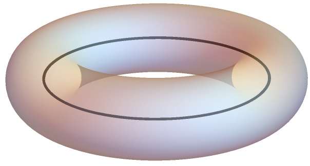
Figure 1: An illustration of a toroidal surface wrapping a circular defect.

Defect RG

The main goal of this work is to study defect renormalization group (DRG) flows. A DRG may be triggered perturbing a DCFT with one or more relevant defect operators. For instance, we may consider a defect operator $\mathcal{O}$ with $\Delta_{\mathcal{O}}<1$:

$$S_{DCFT}\rightarrow S_{DCFT}+M_{0}^{1-\Delta_{\mathcal{O}}}\int_{D}d\sigma\mathcal{O}(\sigma)\,,$$ (5)

where $\int_{D}$ stand for integration along the defect and $M_{0}$ is the mass scale of the flow. Conformal invariance (i.e. $SL(2,\mathbb{R})$ transformations that preserve the defect) is now explicitly broken by the scale $M_{0}$ to just translations along the defect.

Due to the locality of the bulk CFT, the bulk stress tensor remains conserved and traceless (up to possible bulk trace anomalies in curved space) away from the line. However, now a defect stress tensor $T_{D}$ is allowed. In other words, energy can now be stored on the defect. Not only $T_{D}$ is allowed, such an operator must always exist away from the fixed points of the defect. The existence of the operator $T_{D}$ is the reason that $SL(2,\mathbb{R})$ charges are no longer conserved. Since $T_{D}$ is localized to the defect, what we mean by saying that $SL(2,\mathbb{R})$ charges are no longer conserved is that, if the charges are integrated on surfaces that intersect the defect, then they are not invariant under small deformations.

Invariance under translations along the defect implies that eq. (1) in the presence of $T_{D}$ is modified to:

$$\nabla_{\mu}T^{\mu\nu}_{b}=-\delta_{D}^{d-1}\dot{X}^{\nu}\dot{T}_{D}-\delta_{D}^{d-1}n^{\nu}_{i}D^{i}\,,$$ (6)

where $X^{\mu}(\sigma)$ is the embedding function describing the defect location and the dot stands for derivatives with respect to the line coordinate $\sigma$, so that $\dot{X}^{\nu}$ is a tangent vector to the defect. Equation (6) merely expresses the energy balance between the bulk and the defect.

Spurion analysis and the dilaton

As it often happens in the study of RG flows, it is useful to promote the renormalization group scale to a function of position $M(\sigma)=M_{0}e^{\Phi(\sigma)}$ Komargodski:2011xv ; Luty:2012ww , where $\Phi(\sigma)$ is a dimensionless background dilaton field. To linear order, the partition function of the theory depends on the dilaton through to the defect energy-momentum tensor:

$$\log Z|_{\Phi+\delta\Phi}=\log Z|_{\Phi}+\int_{D}d\sigma\delta\Phi(\sigma)\langle T_{D}(\sigma)\rangle_{\Phi}+$$

$$+\frac{1}{2}\int_{D}d\sigma_{1}\int_{D}d\sigma_{2}\delta\Phi(\sigma_{1})\delta\Phi(\sigma_{2})\langle T_{D}(\sigma_{1})T_{D}(\sigma_{2})\rangle_{\Phi}$$

$$+\ldots\,.$$ (7)

The background dilaton field acts a source for the theory. This in turn modifies the conservation equation (6) as follows Osborn:1993cr ; Cuomo:2021cnb

$$\nabla_{\mu}T^{\mu\nu}_{b}=-\delta_{D}^{d-1}\dot{X}^{\nu}\left(\dot{T}_{D}-\dot{\Phi}\,T_{D}\right)-\delta_{D}^{d-1}n^{\nu}_{i}D^{i}\,.$$ (8)

If one views the coordinate along the defect as time, then a nontrivial $\Phi(\sigma)$ renders the theory time dependent and (8) relates the non-conservation rate of the charge associated with translations along the defect with the derivative of the dilaton source.

A position dependent mass scale breaks the $SL(2,\mathbb{R})$ symmetry completely. What we gain by introducing the general background field $\Phi(\sigma)$ is that $SL(2,\mathbb{R})$ allows us to relate different theories instead of directly placing constraints on a given theory. Indeed, we will use eq. (8) in what follows to derive some non-trivial identities relating theories with different values for the source $\Phi(\sigma)$.

RG flows induced by the broken charges

It is crucial to realize that the identity (4) holds irrespectively of the breaking of scale invariance on the defect (i.e. it holds for any $\Phi(\sigma)$). This is because the charges wrapping the defect do not intersect it and hence such charges are oblivious to what happens on the defect and they remain invariant under small deformations. They can be moved off to infinity where they annihilate the vacuum. (To see that, one can realize the wrapping surface as the difference between two $S^{d-1}$ surfaces outside and inside the loop.)

As we explained, on general grounds one expects that $SL(2,\mathbb{R})$ transformation can be reabsorbed into a transformation of the dilaton $\Phi(\sigma)$, leading to relations between different theories. This can be made precise by using eq. (4). To that end, consider shrinking the radius of the topological surface enclosing the defect (see fig. 1). It is clear from Gauss’s law that the only contribution in the integration of the stress tensor arises from the right hand side in eq. (8). We therefore conclude that eq. (4) implies the following relation:

$$\begin{split}0&=Q_{\xi}(D)=\int d^{d-1}\Sigma^{\mu}\langle T_{\mu\nu}^{b}\rangle\xi^{\nu}\\ &=\int_{D}d\sigma\left(\dot{\xi}_{D}+\xi_{D}\dot{\Phi}\right)\langle T_{D}\rangle\,,\end{split}$$ (9)

where in the second line we integrated by parts and we denoted by $\xi_{D}$ the projection of the Killing vectors (3) on the defect. We crucially used the fact that the normal components of the $SL(2,\mathbb{R})$ Killing vectors vanish on the defect. In fact, for more general conformal Killing vectors which do not leave the loop invariant, an analogous identity picks an additional contribution from the displacement operator in eq. (8) but we do not study these identities here.

Due to the linear coupling between the defect stress tensor and the dilaton, we may interpret eq. (9) as an equivalence between defects with different DRG scales $M(\sigma)$:

$$\Phi\sim\Phi+\alpha\left(\dot{\xi}_{D}+\xi_{D}\dot{\Phi}\right)\qquad|\alpha|\ll 1\,,$$ (10)

for any $SL(2,\mathbb{R})$ Killing vector $\xi$ and any infinitesimal $\alpha$. This observation is most useful when considering the expansion of the partition function (7) around $\Phi=0$. Demanding the equivalence (10) at each order in the field expansion we then find an infinite number of identities for the correlation functions of the defect stress tensor. At second order in the field expansion we obtain the following one (omitting the subscript $\Phi=0$ from now on):

$$\int_{D}d\sigma\,\xi_{D}(\sigma)\dot{\Phi}(\sigma)\langle T_{D}(\sigma)\rangle=$$

$$-\int_{D}d\sigma_{1}\int_{D}d\sigma_{2}\,\dot{\xi}_{D}(\sigma_{1})\Phi(\sigma_{2})\langle T_{D}(\sigma_{1})T_{D}(\sigma_{2})\rangle\,.$$ (11)

Crucially, this identity holds for any $\Phi(\sigma)$. Notice that the right hand side of eq. (11) for generic choices of the dilaton profile is naively divergent. Our arguments however ensure that these identities must hold in any regularization scheme which preserves the invariance of the partition function under diffeomorphisms and defect reparametrizations.

At this point it is useful to specify a cylindrical system of coordinates on the defect: $x^{1}=R\cos\phi$, $x^{2}=R\sin\phi$ and set $\sigma=R\phi$. The projection of the three Killing vectors in eq. (3) reads, respectively,

$$\xi_{D}=-\sin\phi~{},\quad\xi_{D}=\cos\phi~{},\quad\xi_{D}=-1~{}.$$ (12)

Eq. (11) is trivial for $\xi_{D}=-1$, but provides non-trivial constraints for the other two choices, which lead to identical constraints. A particularly useful relation is obtained choosing $\xi_{D}=-\sin\phi$ and $\Phi\propto\cos\phi$ in eq. (11). This leads to:

$$R\int_{D}d\phi\langle T_{D}(\phi)\rangle\\ =R^{2}\int_{D}d\phi_{1}\int_{D}d\phi_{2}\langle T_{D}(\phi_{1})T_{D}(\phi_{2})\rangle\cos(\phi_{1}-\phi_{2})\,,$$ (13)

where we used trigonometric identities and invariance under translations along the defect to simplify both sides. Eq. (13) will be very useful in providing a gradient formula for the DRG flow of a suitably defined defect entropy.

The defect entropy

Our discussion thus far focused on defects in flat space, but all our considerations apply on all conformally equivalent manifolds. These include the $d$-dimensional sphere of radius $R$, with the defect spanning a maximal circle, and the cylinder $\mathds{R}\times S^{d-1}$, with the defect on the equator of $S^{d-1}$ at a fixed value of the Euclidean time $\tau=\log x^{2}/R=0$.

We can use any of these geometries to define a defect $g$-function, $g(M_{0}R)$, in terms of the partition function in the presence of the defect, normalized by the partition function without it:

$$\log g(M_{0}R)=\log Z_{\mathcal{M}}-\log Z^{(CFT)}_{\mathcal{M}}\,,$$ (14)

where $\log Z^{(CFT)}_{\mathcal{M}}$ is the partition function of the theory without the defect. The defect contribution $g$ depends only on the dimensionless product $M_{0}R$ and it reduces to a constant at the fixed points (in a sense that we will explain below).

We must now ask to what extent is $g$ well defined at the fixed points and away from them. $\log g$ can be shifted by the addition of a cosmological constant counterterm $\int d\sigma M_{0}\sim M_{0}R$ with an arbitrary coefficient. All other nontrivial geometric invariants which are analytic around the flat metric have dimension larger than one and cannot appear as counterterms. Therefore no additional ambiguities exist in $d>2$ (we will discuss $d=2$ more in detail below). Therefore, one can obtain a scheme-indepdent quantity which we will refer to as the defect entropy, defined as:

$$s(M_{0}R)=\left(1-R\frac{\partial}{\partial R}\right)\log g(M_{0}R)\,.$$ (15)

At the fixed points, $s(M_{0}R)$ is a pure number which is scheme independent. It is equal to the perimeter-independent contribution to $\log g(M_{0}R)$ at the fixed point. We will refer to these fixed point values of $g$ as $g_{UV},g_{IR}$, respectively. We will show that $s(M_{0}R)$ decreases monotonically under DRG, implying $g_{UV}>g_{IR}$.

In $d=2$ eq. (15) coincides with the interface contribution to the thermal entropy of the theory. To make the connection with $d=2$ precise, one needs to remember that in $d=2$ we can also allow the counterterm $\int d\sigma K$, where $K$ is the extrinsic curvature. Such a term vanishes for a maximal circle in $S^{2}$ and on $\mathbb{R}\times S^{1}$ and therefore all our conclusions hold unaltered on those manifolds. Furthermore $CPT$ invariance implies that the coefficient of this counterterm should be purely imaginary. Therefore the definition in eq. (15) is meaningful also in flat space provided we focus on the real part of the defect entropy.

The gradient formula

We now have all the ingredients to derive a gradient formula for the DRG flow of the defect entropy. Since $g$ depends on $M_{0}R$ only, for constant dilaton $\Phi$, it follows that $g$ depends on the combination $RM_{0}e^{\Phi}$. We may therefore write the variation of the defect entropy $s$ under a change in the mass scale as follows:

$$M_{0}\frac{\partial}{\partial M_{0}}s(M_{0}R)=\left[\left(\frac{d}{d\Phi}-\frac{d^{2}}{d\Phi^{2}}\right)\log g\left(RM_{0}e^{\Phi}\right)\right]_{\Phi=0}\,.$$ (16)

Using the expansion (7) for constant $\Phi$ we then can write eq. (16) in terms of correlation functions of the defect stress tensor

$$\begin{split}M_{0}\frac{\partial}{\partial M_{0}}s(M_{0}R)&=R\int_{D}d\phi\,\langle T_{D}(\phi)\rangle\\ &-R^{2}\int_{D}d\phi_{1}\int_{D}d\phi_{2}\langle T_{D}(\phi_{1})T_{D}(\phi_{2})\rangle\,.\end{split}$$ (17)

Eq. (17) may not seem very useful at first sight. It is not manifestly sign-definite, nor is it manifestly finite. To clarify these issues, we can rewrite the first term using eq. (13). We obtain:

$$M_{0}\frac{\partial s}{\partial M_{0}}=$$ (18)

$$-R^{2}\int_{D}d\phi_{1}\int_{D}d\phi_{2}\langle T_{D}(\phi_{1})T_{D}(\phi_{2})\rangle\left[1-\cos\left(\phi_{1}-\phi_{2}\right)\right]\,.$$

The right hand side of (18) is free of divergences and ambiguities due to the double zero of $1-\cos\left(\phi_{1}-\phi_{2}\right)$. Furthermore, (18) is manifestly negative in a reflection positive theory (note that this also applies to a connected 2-point function, as on the right hand side of (18)). Therefore, we deduce that $s$ monotonically decreases along defect RG flows, implying that the UV and IR DCFT satisfy

$$g_{UV}>g_{IR}\,.$$ (19)

Eq. (18) additionally implies that $s$ does does no depend on the marginal parameters on the defect.

In $d=2$, equation (19) was originally conjectured to hold for boundaries (and therefore, using the folding trick, for interfaces) by Affleck and Ludwig Affleck:1991tk ; Affleck:1992ng . In $d=2$, in the regime where the DRG flow can be described in terms of finitely many couplings and beta functions, a gradient formula equivalent to eq. (18) was proposed in the context of string field theory Witten:1992qy ; Witten:1992cr ; Shatashvili:1993kk ; Shatashvili:1993ps ; Kutasov:2000qp . It was then established by Friedan and Konechny Friedan:2003yc . An alternative proof of eq. (19) in $d=2$ was also given Casini:2016fgb using quantum information methods. Our work provides an extension of those results to line defects in an arbitrary number of dimensions. We also remark that the inequality (19) was recently conjectured in Kobayashi:2018lil for arbitrary $d$. Another remark is that the trivial line has $g=1$. However, it may a priori be that $g<1$ for some non-trivial lines, as sometimes happens in $2d$ Oshikawa:1996dj ; Oshikawa:1996ww .

Eq. (19) was extensively checked in $d=2$, see e.g. Affleck:1991tk ; Affleck:1992ng ; Affleck:1995ge ; Konechny:2003yy . We additionally verified our results (18) and (19) in sevaral concrete examples, including a flow between Wilson lines in $\mathcal{N}=4$ SYM previously studied in Polchinski:2011im ; Beccaria:2017rbe . Details can be found in the Supplemental Material.

Finally, we remark that the partition function of higher-dimensional defects is subject to further ambiguities besides a cosmological constant, rendering a generalization of our arguments not straightforward. For two- and four-dimensional defects irreversibility of the DRG flow was proven via different means, using Weyl anomaly matching Jensen:2015swa ; Wang:2021mdq .

Acknowledgements

We acknowledge useful discussions with Bartolomeu Fiol, Sergei Gukov, Simeon Hellerman, Márk Mezei, Luigi Tizzano, Cumrun Vafa, and Yifan Wang. GC is supported by the Simons Foundation (Simons Collaboration on the Non-perturbative Bootstrap) grants 488647 and 397411. ZK and ARM are supported in part by the Simons Foundation grant 488657 (Simons Collaboration on the Non-Perturbative Bootstrap) and the BSF grant no. 2018204. The work of ARM was also supported in part by the Zuckerman-CHE STEM Leadership Program.

Appendix A Supplemental Material

A.1 A. Subtleties for the infinite line geometry

Naively, a defect on an infinite straight line is conformally equivalent to a circular defect. However, there is a subtlety associated to the infinite extent of the straight line defect. Here we detail this issue.

To explain the subtlety with straight line defects, consider a defect $D$ which extends in the $d$th direction at $x^{i}=0$, where $i,j,\ldots$ denote indices $1,\ldots,d-1$ transverse to the line. For $d>2$, the one-point function of the stress tensor depends on a constant $h_{D}$ and reads Kapustin:2005py :

$$\begin{gathered}\langle T^{dd}(x)\rangle=h_{D}\frac{d-2}{r^{d}}\,,\quad\langle T^{id}(x)\rangle=0\,,\\ \langle T^{ij}(x)\rangle=-h_{D}\frac{(2\,\delta^{ij}-d\,x^{i}x^{j}/r^{2})}{r^{d}}\,,\end{gathered}$$ (20)

where $r^{2}=x^{i}x^{i}$ is the distance from the line operator (we assume that the defect has zero transverse spin for simplicity).

Eq. (20) is covariant under conformal transformations. However, a subtlety arises when we consider the expectation values of the $SL(2,\mathbb{R})$ charges. The expectation values of the charges are obtained by integrating the stress tensor contracted with the appropriate Killing vector at a fixed distance $\varepsilon$ on a cylinder around the defect:

$$Q_{\xi}(D)=\int_{r=\varepsilon}d^{d-1}\Sigma^{\mu}\langle T^{b}_{\mu\nu}\rangle\xi^{\nu}\,.$$ (21)

For the dilation and special conformal Killing vectors along the line one finds a result proportional to $1/\varepsilon$ times a linearly divergent integral $\int dx^{d}$. This is in sharp contrast with the expected charge conservation. Technically, this is because the $x\rightarrow\infty$ limit of the stress tensor depends on the distance $r$ from the defect, and it is therefore not single-valued at the point at infinity. This implies that that the conformal charges vanish only when the distance between the integration surface and the defect diverges sufficiently fast as $x^{d}\rightarrow\pm\infty$. This problem with the conformal charges is presumably related to the disagreement between the expectation value of circular and linear Maldacena-Wilson loops in $\mathcal{N}=4$ SYM Erickson:2000af ; Drukker:2000rr ; Pestun:2007rz .

A.2 B. Examples

The inequality $g_{UV}>g_{IR}$ was extensively checked in the literature in $d=2$. Early examples include flows between the free and the fixed boundary conditions in the Ising model Affleck:1991tk and the weak to strong coupling flow in the Kondo effect Affleck:1992ng ; Affleck:1995ge . In $d>2$ flows between various Wilson lines in 4 dimensions and a vast class of holographic flows was considered in Kobayashi:2018lil . The results are consistent with the monotonicity of $g$.

Let us now discuss the gradient formula:

$$M_{0}\frac{\partial s}{\partial M_{0}}=$$ (22)

$$-R^{2}\int_{D}d\phi_{1}\int_{D}d\phi_{2}\langle T_{D}(\phi_{1})T_{D}(\phi_{2})\rangle\left[1-\cos\left(\phi_{1}-\phi_{2}\right)\right]\,,$$

where $s$ is the defect entropy defined in the main text. We verified eq. (22) in two concrete examples: conformal perturbation theory and the flow from a standard Wilson loop to a supersymmetric one in $\mathcal{N}=4$ SYM, proposed by Polchinski and Sully Polchinski:2011im , at weak ’t Hooft coupling.

In conformal perturbation theory, one starts from an abstract DCFT and perturbs it with one or more weakly or marginally relevant operators; one then computes the partition function expanding in the couplings of the perturbations. It is then simple to compute the defect entropy and verify the gradient formula (22) using $T_{D}=\beta_{i}\mathcal{O}_{i}$, where $\beta_{i}$ are the beta functions of the defect coupling and $\mathcal{O}_{i}$ the defect operators with which the DCFT is deformed. In this setup, in $d=2$, eq. (22) was verified to third order in perturbation theory in Konechny:2003yy . A similar argument holds for any $d$.

Let us now consider the DRG flow from the ordinary Wilson loop (WL) to the $1/2$ BPS Wilson-Maldacena loop (WML) in $\mathcal{N}=4$ SYM in four dimensions in the planar limit. This was proposed in Polchinski:2011im and studied in detail in Beccaria:2017rbe . One considers a single-parameter family of Wilson loop operators in the fundamental representation

$$W^{(\zeta)}=\frac{1}{N}\text{Tr}\,\mathcal{P}\,\text{exp}\,\oint_{C}d\tau\left[iA_{\mu}(x)\dot{x}^{\mu}+\zeta\Phi_{m}(x)\theta^{m}|\dot{x}|\right],$$ (23)

where $\theta_{m}^{2}=1$, $\zeta$ is the coefficient in front of the scalar coupling ($m=1,\cdots,6$) and we follow closely the notations of Beccaria:2017rbe , focusing on circular contours. The theory admits a UV fixed point $\zeta=0$ and may flow to the WML ($|\zeta|=1$), that provides an IR stable fixed point. Generically, the expectation values of the Wilson loop operators depend on the renormalization scale through:

$$\langle W^{(\zeta)}\rangle\equiv W\left(\lambda;\zeta(M_{0}R),M_{0}R\right),$$ (24)

$$M_{0}\frac{\partial}{\partial M_{0}}W+\beta_{\zeta}\frac{\partial}{\partial\zeta}W=0,$$

where we note that the boundary coupling $\zeta$ depends on the renormalization scale $\zeta=\zeta(M_{0}R)$. Here $\langle W^{(\zeta)}\rangle$ stands for the $g$-function of the defect. At weak ’t Hooft coupling, $\lambda\ll 1$, this dependence follows from the beta function of $\zeta$ Polchinski:2011im :

$$\beta_{\zeta}=M_{0}\frac{\partial\zeta}{\partial M_{0}}=-\frac{\lambda}{8\pi^{2}}\zeta\left(1-\zeta^{2}\right)+\mathcal{O}\left(\lambda^{2}\right)\,.$$ (25)

The partition function of the DCFT was evaluated to order $\mathcal{O}(\lambda^{2})$ in Beccaria:2017rbe , where it was found that (in units such that $R=1$):

$$\langle W^{(\zeta)}\rangle=1+\frac{1}{8}\lambda+\left[\frac{1}{192}+\frac{1}{128\pi^{2}}\left(1-\zeta^{2}\right)^{2}\right]\lambda^{2}+\mathcal{O}(\lambda^{3})\,.$$ (26)

Notice that these results, though perturbative in $\lambda$, are exact throughout the flow. From eq. (26) one clearly reads $g_{UV}>g_{IR}$. Upon taking derivatives with respect to $M_{0}$ and using eq. (25), one may then compute the DRG gradient of the defect entropy to be:

$$M_{0}\frac{\partial s}{\partial M_{0}}=-\frac{\lambda^{3}}{256\pi^{4}}\zeta^{2}\left(1-\zeta^{2}\right)^{2}\,+\mathcal{O}\left(\lambda^{4}\right).$$ (27)

Hence $s$ monotonically decreases along the DRG flow. Furthermore, since to the order we are working we may neglect anomalous dimensions, we easily find the two-point function of the defect stress tensor Beccaria:2017rbe :

$$\langle T_{D}(\phi)T_{D}(0)\rangle=\frac{\lambda}{8\pi^{2}}\frac{\beta_{\zeta}^{2}}{\left(2\sin\frac{\phi}{2}\right)^{2}}\left[1+\mathcal{O}\left(\lambda\right)\right]\,.$$ (28)

It is then simple to use this equation and the beta-function (25) to verify explicitly the agreement of the RHS of the gradient formula (22) with the expression (27). This provides a test of the gradient formula (22) in the small ’t Hooft coupling regime.

In the strong coupling regime one expects a similar DRG flow to take place. This is supported by the holographic calculation of the DCFT partition functions at the fixed points, whose ratio satisfies $\langle W^{(0)}\rangle/\langle W^{(1)}\rangle\sim\lambda^{2}$ for $\lambda\gg 1$ Beccaria:2017rbe .

References

- (1) A. B. Zomolodchikov, “Irreversibility” of the flux of the renormalization group in a 2D field theory, Soviet Journal of Experimental and Theoretical Physics Letters 43 (1986) 730.
- (2) J. L. Cardy, Is There a c Theorem in Four-Dimensions?, Phys. Lett. B 215 (1988) 749.
- (3) A. Cappelli, D. Friedan and J. I. Latorre, C theorem and spectral representation, Nucl. Phys. B 352 (1991) 616.
- (4) H. Osborn, Weyl consistency conditions and a local renormalization group equation for general renormalizable field theories, Nucl. Phys. B 363 (1991) 486.
- (5) R. C. Myers and A. Sinha, Holographic c-theorems in arbitrary dimensions, JHEP 01 (2011) 125 [1011.5819].
- (6) D. L. Jafferis, I. R. Klebanov, S. S. Pufu and B. R. Safdi, Towards the F-Theorem: N=2 Field Theories on the Three-Sphere, JHEP 06 (2011) 102 [1103.1181].
- (7) Z. Komargodski and A. Schwimmer, On Renormalization Group Flows in Four Dimensions, JHEP 12 (2011) 099 [1107.3987].
- (8) H. Casini and M. Huerta, On the RG running of the entanglement entropy of a circle, Phys. Rev. D 85 (2012) 125016 [1202.5650].
- (9) H. Elvang, D. Z. Freedman, L.-Y. Hung, M. Kiermaier, R. C. Myers and S. Theisen, On renormalization group flows and the a-theorem in 6d, JHEP 10 (2012) 011 [1205.3994].
- (10) H. Elvang and T. M. Olson, RG flows in d dimensions, the dilaton effective action, and the a-theorem, JHEP 03 (2013) 034 [1209.3424].
- (11) K. Yonekura, Perturbative c-theorem in d-dimensions, JHEP 04 (2013) 011 [1212.3028].
- (12) O. Antipin, M. Gillioz, E. Mølgaard and F. Sannino, The a theorem for gauge-Yukawa theories beyond Banks-Zaks fixed point, Phys. Rev. D 87 (2013) 125017 [1303.1525].
- (13) B. Grinstein, A. Stergiou and D. Stone, Consequences of Weyl Consistency Conditions, JHEP 11 (2013) 195 [1308.1096].
- (14) I. Jack and H. Osborn, Constraints on RG Flow for Four Dimensional Quantum Field Theories, Nucl. Phys. B 883 (2014) 425 [1312.0428].
- (15) F. Baume, B. Keren-Zur, R. Rattazzi and L. Vitale, The local Callan-Symanzik equation: structure and applications, JHEP 08 (2014) 152 [1401.5983].
- (16) B. Grinstein, D. Stone, A. Stergiou and M. Zhong, Challenge to the Theorem in Six Dimensions, Phys. Rev. Lett. 113 (2014) 231602 [1406.3626].
- (17) S. Giombi and I. R. Klebanov, Interpolating between and , JHEP 03 (2015) 117 [1409.1937].
- (18) I. Jack, D. R. T. Jones and C. Poole, Gradient flows in three dimensions, JHEP 09 (2015) 061 [1505.05400].
- (19) C. Cordova, T. T. Dumitrescu and K. Intriligator, Anomalies, renormalization group flows, and the a-theorem in six-dimensional (1, 0) theories, JHEP 10 (2016) 080 [1506.03807].
- (20) H. Casini, M. Huerta, R. C. Myers and A. Yale, Mutual information and the F-theorem, JHEP 10 (2015) 003 [1506.06195].
- (21) S. S. Pufu, The F-Theorem and F-Maximization, J. Phys. A 50 (2017) 443008 [1608.02960].
- (22) H. Casini, E. Testé and G. Torroba, Markov Property of the Conformal Field Theory Vacuum and the a Theorem, Phys. Rev. Lett. 118 (2017) 261602 [1704.01870].
- (23) M. Fluder and C. F. Uhlemann, Evidence for a 5d F-theorem, JHEP 02 (2021) 192 [2011.00006].
- (24) L. V. Delacretaz, A. L. Fitzpatrick, E. Katz and M. T. Walters, Thermalization and Hydrodynamics of Two-Dimensional Quantum Field Theories, 2105.02229.
- (25) A. Kapustin, Wilson-’t Hooft operators in four-dimensional gauge theories and S-duality, Phys. Rev. D 74 (2006) 025005 [hep-th/0501015].
- (26) J. Gomis and F. Passerini, Holographic Wilson Loops, JHEP 08 (2006) 074 [hep-th/0604007].
- (27) M. Billó, M. Caselle, D. Gaiotto, F. Gliozzi, M. Meineri and R. Pellegrini, Line defects in the 3d Ising model, JHEP 07 (2013) 055 [1304.4110].
- (28) D. Gaiotto, D. Mazac and M. F. Paulos, Bootstrapping the 3d Ising twist defect, JHEP 03 (2014) 100 [1310.5078].
- (29) S. Giombi, E. Helfenberger, Z. Ji and H. Khanchandani, Monodromy Defects from Hyperbolic Space, 2102.11815.
- (30) S. Liu, H. Shapourian, A. Vishwanath and M. A. Metlitski, Magnetic impurities at quantum critical points: large- expansion and SPT connections, 2104.15026.
- (31) A. Tsvelick and P. Wiegmann, Exact solution of the multichannel kondo problem, scaling, and integrability, Journal of Statistical Physics 38 (1985) 125.
- (32) I. Affleck and A. W. W. Ludwig, Exact conformal-field-theory results on the multichannel Kondo effect: Single-fermion Green’s function, self-energy, and resistivity, Phys. Rev. B 48 (1993) 7297.
- (33) I. Affleck, Conformal field theory approach to the Kondo effect, Acta Phys. Polon. B 26 (1995) 1869 [cond-mat/9512099].
- (34) S. Sachdev, C. Buragohain and M. Vojta, Quantum impurity in a nearly critical two-dimensional antiferromagnet, Science 286 (1999) 2479.
- (35) M. Vojta, C. Buragohain and S. Sachdev, Quantum impurity dynamics in two-dimensional antiferromagnets and superconductors, Physical Review B 61 (2000) 15152.
- (36) I. Affleck and A. W. W. Ludwig, Universal noninteger ’ground state degeneracy’ in critical quantum systems, Phys. Rev. Lett. 67 (1991) 161.
- (37) P. Dorey, I. Runkel, R. Tateo and G. Watts, g function flow in perturbed boundary conformal field theories, Nucl. Phys. B 578 (2000) 85 [hep-th/9909216].
- (38) S. Yamaguchi, Holographic RG flow on the defect and g theorem, JHEP 10 (2002) 002 [hep-th/0207171].
- (39) D. Friedan and A. Konechny, On the boundary entropy of one-dimensional quantum systems at low temperature, Phys. Rev. Lett. 93 (2004) 030402 [hep-th/0312197].
- (40) T. Azeyanagi, A. Karch, T. Takayanagi and E. G. Thompson, Holographic calculation of boundary entropy, JHEP 03 (2008) 054 [0712.1850].
- (41) T. Takayanagi, Holographic Dual of BCFT, Phys. Rev. Lett. 107 (2011) 101602 [1105.5165].
- (42) J. Estes, K. Jensen, A. O’Bannon, E. Tsatis and T. Wrase, On Holographic Defect Entropy, JHEP 05 (2014) 084 [1403.6475].
- (43) D. Gaiotto, Boundary F-maximization, 1403.8052.
- (44) K. Jensen and A. O’Bannon, Constraint on Defect and Boundary Renormalization Group Flows, Phys. Rev. Lett. 116 (2016) 091601 [1509.02160].
- (45) H. Casini, I. Salazar Landea and G. Torroba, The g-theorem and quantum information theory, JHEP 10 (2016) 140 [1607.00390].
- (46) N. Andrei et al., Boundary and Defect CFT: Open Problems and Applications, J. Phys. A 53 (2020) 453002 [1810.05697].
- (47) N. Kobayashi, T. Nishioka, Y. Sato and K. Watanabe, Towards a -theorem in defect CFT, JHEP 01 (2019) 039 [1810.06995].
- (48) H. Casini, I. Salazar Landea and G. Torroba, Irreversibility in quantum field theories with boundaries, JHEP 04 (2019) 166 [1812.08183].
- (49) S. Giombi and H. Khanchandani, CFT in AdS and boundary RG flows, JHEP 11 (2020) 118 [2007.04955].
- (50) Y. Wang, Surface Defect, Anomalies and -Extremization, 2012.06574.
- (51) T. Nishioka and Y. Sato, Free energy and defect -theorem in free scalar theory, JHEP 05 (2021) 074 [2101.02399].
- (52) Y. Wang, Defect -Theorem and -Maximization, 2101.12648.
- (53) Y. Sato, Free energy and defect -theorem in free fermion, JHEP 05 (2021) 202 [2102.11468].
- (54) Y. Nakayama, Is boundary conformal in CFT?, Phys. Rev. D 87 (2013) 046005 [1210.6439].
- (55) C. P. Herzog and K.-W. Huang, Boundary Conformal Field Theory and a Boundary Central Charge, JHEP 10 (2017) 189 [1707.06224].
- (56) G. Cuomo, M. Mezei and A. Raviv-Moshe, Boundary Conformal Field Theory at Large Charge, 2108.06579.
- (57) H. Osborn and A. C. Petkou, Implications of conformal invariance in field theories for general dimensions, Annals Phys. 231 (1994) 311 [hep-th/9307010].
- (58) F. Gliozzi, P. Liendo, M. Meineri and A. Rago, Boundary and Interface CFTs from the Conformal Bootstrap, JHEP 05 (2015) 036 [1502.07217].
- (59) P. Liendo, L. Rastelli and B. C. van Rees, The Bootstrap Program for Boundary CFTd, JHEP 07 (2013) 113 [1210.4258].
- (60) M. Billò, V. Gonçalves, E. Lauria and M. Meineri, Defects in conformal field theory, JHEP 04 (2016) 091 [1601.02883].
- (61) E. Lauria, P. Liendo, B. C. Van Rees and X. Zhao, Line and surface defects for the free scalar field, JHEP 01 (2021) 060 [2005.02413].
- (62) A. A. Belavin, A. M. Polyakov and A. B. Zamolodchikov, Infinite Conformal Symmetry in Two-Dimensional Quantum Field Theory, Nucl. Phys. B 241 (1984) 333.
- (63) R. Rattazzi, V. S. Rychkov, E. Tonni and A. Vichi, Bounding scalar operator dimensions in 4D CFT, JHEP 12 (2008) 031 [0807.0004].
- (64) D. Poland, S. Rychkov and A. Vichi, The Conformal Bootstrap: Theory, Numerical Techniques, and Applications, Rev. Mod. Phys. 91 (2019) 015002 [1805.04405].
- (65) D. Correa, J. Henn, J. Maldacena and A. Sever, An exact formula for the radiation of a moving quark in N=4 super Yang Mills, JHEP 06 (2012) 048 [1202.4455].
- (66) F. Fucito, J. F. Morales and R. Poghossian, Wilson loops and chiral correlators on squashed spheres, JHEP 11 (2015) 064 [1507.05426].
- (67) B. Fiol, E. Gerchkovitz and Z. Komargodski, Exact Bremsstrahlung Function in Superconformal Field Theories, Phys. Rev. Lett. 116 (2016) 081601 [1510.01332].
- (68) L. Bianchi, M. Lemos and M. Meineri, Line Defects and Radiation in Conformal Theories, Phys. Rev. Lett. 121 (2018) 141601 [1805.04111].
- (69) L. Bianchi, M. Billò, F. Galvagno and A. Lerda, Emitted Radiation and Geometry, JHEP 01 (2020) 075 [1910.06332].
- (70) N. B. Agmon and Y. Wang, Classifying Superconformal Defects in Diverse Dimensions Part I: Superconformal Lines, 2009.06650.
- (71) J. K. Erickson, G. W. Semenoff and K. Zarembo, Wilson loops in N=4 supersymmetric Yang-Mills theory, Nucl. Phys. B 582 (2000) 155 [hep-th/0003055].
- (72) N. Drukker and D. J. Gross, An Exact prediction of N=4 SUSYM theory for string theory, J. Math. Phys. 42 (2001) 2896 [hep-th/0010274].
- (73) V. Pestun, Localization of gauge theory on a four-sphere and supersymmetric Wilson loops, Commun. Math. Phys. 313 (2012) 71 [0712.2824].
- (74) J. Gomis, S. Matsuura, T. Okuda and D. Trancanelli, Wilson loop correlators at strong coupling: From matrices to bubbling geometries, JHEP 08 (2008) 068 [0807.3330].
- (75) N. Ishibashi, The Boundary and Crosscap States in Conformal Field Theories, Mod. Phys. Lett. A 4 (1989) 251.
- (76) J. L. Cardy, Boundary Conditions, Fusion Rules and the Verlinde Formula, Nucl. Phys. B 324 (1989) 581.
- (77) Z. Komargodski, The Constraints of Conformal Symmetry on RG Flows, JHEP 07 (2012) 069 [1112.4538].
- (78) M. A. Luty, J. Polchinski and R. Rattazzi, The -theorem and the Asymptotics of 4D Quantum Field Theory, JHEP 01 (2013) 152 [1204.5221].
- (79) A. Lewkowycz and J. Maldacena, Exact results for the entanglement entropy and the energy radiated by a quark, JHEP 05 (2014) 025 [1312.5682].
- (80) T. Grover, A. M. Turner and A. Vishwanath, Entanglement Entropy of Gapped Phases and Topological Order in Three dimensions, Phys. Rev. B 84 (2011) 195120 [1108.4038].
- (81) H. Liu and M. Mezei, A Refinement of entanglement entropy and the number of degrees of freedom, JHEP 04 (2013) 162 [1202.2070].
- (82) E. Witten, On background independent open string field theory, Phys. Rev. D 46 (1992) 5467 [hep-th/9208027].
- (83) E. Witten, Some computations in background independent off-shell string theory, Phys. Rev. D 47 (1993) 3405 [hep-th/9210065].
- (84) S. L. Shatashvili, Comment on the background independent open string theory, Phys. Lett. B 311 (1993) 83 [hep-th/9303143].
- (85) S. L. Shatashvili, On the problems with background independence in string theory, Alg. Anal. 6 (1994) 215 [hep-th/9311177].
- (86) D. Kutasov, M. Marino and G. W. Moore, Some exact results on tachyon condensation in string field theory, JHEP 10 (2000) 045 [hep-th/0009148].
- (87) J. Erdmenger, C. Hoyos, A. O’Bannon and J. Wu, A Holographic Model of the Kondo Effect, JHEP 12 (2013) 086 [1310.3271].
- (88) M. Oshikawa and I. Affleck, Boundary conformal field theory approach to the critical two-dimensional Ising model with a defect line, Nucl. Phys. B 495 (1997) 533 [cond-mat/9612187].
- (89) M. Oshikawa and I. Affleck, Defect lines in the Ising model and boundary states on orbifolds, Phys. Rev. Lett. 77 (1996) 2604 [hep-th/9606177].
- (90) J. Polchinski and J. Sully, Wilson Loop Renormalization Group Flows, JHEP 10 (2011) 059 [1104.5077].
- (91) A. Konechny, g function in perturbation theory, Int. J. Mod. Phys. A 19 (2004) 2545 [hep-th/0310258].
- (92) M. Beccaria, S. Giombi and A. Tseytlin, Non-supersymmetric Wilson loop in = 4 SYM and defect 1d CFT, JHEP 03 (2018) 131 [1712.06874].
- (93) S. Elitzur, E. Rabinovici and G. Sarkissian, On least action D-branes, Nucl. Phys. B 541 (1999) 246 [hep-th/9807161].
- (94) S. Fredenhagen, M. R. Gaberdiel and C. A. Keller, Bulk induced boundary perturbations, J. Phys. A 40 (2007) F17 [hep-th/0609034].
- (95) S. Elitzur, B. Karni and E. Rabinovici, Induced Boundary Flow on the c = 1 Orbifold Moduli Space, J. Phys. A 45 (2012) 455401 [1209.4344].
- (96) L. Bianchi, Marginal deformations and defect anomalies, Phys. Rev. D 100 (2019) 126018 [1907.06193].
- (97) C. P. Herzog and I. Shamir, How a-type anomalies can depend on marginal couplings, Phys. Rev. Lett. 124 (2020) 011601 [1907.04952].
- (98) D. R. Green, M. Mulligan and D. Starr, Boundary Entropy Can Increase Under Bulk RG Flow, Nucl. Phys. B 798 (2008) 491 [0710.4348].