Batch Normalization Preconditioning for Neural Network Training

Abstract

Batch normalization (BN) is a popular and ubiquitous method in deep learning that has been shown to decrease training time and improve generalization performance of neural networks. Despite its success, BN is not theoretically well understood. It is not suitable for use with very small mini-batch sizes or online learning. In this paper, we propose a new method called Batch Normalization Preconditioning (BNP). Instead of applying normalization explicitly through a batch normalization layer as is done in BN, BNP applies normalization by conditioning the parameter gradients directly during training. This is designed to improve the Hessian matrix of the loss function and hence convergence during training. One benefit is that BNP is not constrained on the mini-batch size and works in the online learning setting. Furthermore, its connection to BN provides theoretical insights on how BN improves training and how BN is applied to special architectures such as convolutional neural networks. For a theoretical foundation, we also present a novel Hessian condition number based convergence theory for a locally convex but not strong-convex loss, which is applicable to networks with a scale-invariant property.

Keywords: Deep neural networks, Convolutional neural networks, Preconditioning, Batch Normalization

1 Introduction

Batch normalization (BN) is one of the most widely used techniques to improve neural network training. It was originally designed in Ioffe and Szegedy (2015) to address internal covariate shift. It has been found to increase network robustness with respect to parameter and learning rate initialization, to decrease training times, and to improve network regularization. Over the years, BN has become a standard technique in deep learning but the theoretical understanding of BN is still limited. There have been many papers that analyze various properties of BN but some important issues remain unaddressed.

In this paper, we develop a method called Batch Normalization Preconditioning (BNP). Instead of using mini-batch statistics to normalize hidden variables as in BN, BNP uses these statistics to transform the trainable parameters through preconditioning, which improves the conditioning of the Hessian of the loss function and hence accelerates convergence. This is implicitly done by applying a transformation on the gradients during training. Preconditioning is a general technique in numerical analysis (Saad, 2003) that uses a parameter transformation to accelerate convergence of iterative methods. Here, we show that potentially large differences in variances of hidden variables over a mini-batch adversely affect the conditioning of the Hessian. We then derive a suitable parameter transformation that is equivalent to normalizing the hidden variables.

Both BN and BNP use mini-batch statistics to accelerate convergence but the key difference is that BNP does not change the network architecture, but instead uses the mini-batch statistics in an equivalent transformation of parameters to accelerate convergence. In particular, BNP may use statistics computed from a larger dataset rather than the mini-batches. In contrast, BN has the mini-batch statistics embedded in the architecture. This has the advantage of allowing gradients to pass through these statistics during training but this is also a theoretical disadvantage because the training network is dependent on the mini-batch inputs. In particular, the inference network (with a single input) is different from the training network (with mini-batch inputs). This may pose a challenge in implementation with small mini-batches as well as in analysis, even though BN largely works well in practice. We outline our main contributions below:

• We develop a novel Hessian condition number based convergence theory for a locally convex but not strong-convex loss, which is applicable to networks with a scale-invariant property (Neyshabur et al. (2015b); Meng et al. (2019)).

• Under certain conditions, BNP is equivalent to BN. Because of this equivalency, the theoretical basis of BNP provides an explanation of why BN works.

• While BNP has a performance comparable to BN in general, it outperforms BN in the situation of very small mini-batch sizes or online learning where BN is known to have difficulties.

• BN has been adapted to special architectures like convolutional neural networks (CNNs) (Ioffe and Szegedy, 2015) and recurrent neural networks (RNNs) (Laurent et al., 2016; Cooijmans et al., 2016) but the computation of the required mini-batch statistics is more nuanced. For example, in CNNs the mean and variance across the mini-batch and spatial dimensions are used without clear justification. Derivation of BNP for CNNs naturally leads to using these statistics and provides a theoretical understanding of how BN should be applied to CNNs.

Throughout the paper, $\|\cdot\|$ denotes the 2-norm. If $A$ is a square and invertible matrix, $\kappa(A)=\|A\|\|A^{-1}\|$ denotes the condition number of $A$. For a singular or rectangular matrix $A$, we define the condition number as $\kappa(A)=\frac{\sigma_{\text{max}}}{\sigma^{*}_{\text{min}}}$ , where $\sigma^{*}_{\text{min}}$ is the smallest nonzero singular value of $A$ and $\sigma_{\text{max}}$ the largest singular value of $A$. All vectors refer to column vectors. A diagonal matrix with diagonal entries given by the vector $v$ is denoted by diag$(v)$, and $e=[1,1,\cdots,1]^{T}$ denotes the vector of ones with a suitable dimension. All functions and operations of vectors are applied elementwise.

In Section 2, we present BN and various related works. We introduce preconditioned gradient descent in Section 3.1 followed by a Hessian based convergence theory for convex but not strongly-convex losses in Section 3.2. We derive the BNP method in Section 3.3. We discuss the connection between BN and BNP in Section 3.4 and derive BNP for CNNs in Section 4. Finally, we provide experimental results in Section 5. Proofs of most results are given in the appendix.

2 Batch Normalization and Related Work

Consider a fully connected multi-layer neural network in which the $\ell$-th hidden layer is defined by

$$h^{(\ell)}=g(W^{(\ell)}h^{(\ell-1)}+b^{(\ell)}),$$ (1)

where $h^{(0)}$ is the network input $x$, $g$ is an elementwise nonlinear function, and $h^{(\ell)}\in\mathbb{R}^{n_{\ell}}$ is the $\ell$-th hidden variable with $W^{(\ell)}$ and $b^{(\ell)}$ being the associated weight and bias. We refer to such a network as a vanilla network. During training, let $\{x_{1},x_{2},\ldots,x_{N}\}$ be a mini-batch consisting of $N$ examples and $H=[h^{(\ell-1)}_{1},h^{(\ell-1)}_{2},\ldots,h^{(\ell-1)}_{N}]^{T}$ the matrix of associated hidden variables of layer $\ell-1$. BN replaces the $\ell$-th hidden layer by

$$h^{(\ell)}=g\left(W^{(\ell)}\mathcal{B}_{\beta,\gamma}(h^{(\ell-1)})+b^{(\ell)}\right);\hskip 5.69046pt\mathcal{B}_{\beta,\gamma}\left(h^{(\ell-1)}\right)=\gamma\frac{h^{(\ell-1)}-\mu_{H}}{\sigma_{H}}+\beta$$ (2)

where $\sigma_{H}$ and $\mu_{H}$ are the standard deviation and mean vectors of $\{h^{(\ell-1)}_{i}\}$ (i.e. the rows of $H$) and $\gamma,\beta$ are the respective trainable re-scaling and re-centering parameter vectors. The BN transformation operator $\mathcal{B}_{\beta,\gamma}\left(\cdot\right)$ first normalizes the activation $h^{(\ell-1)}$ and then re-scales and re-centers it with $\gamma$ and $\beta$; see Algorithm 1 for details. In practice, the denominator in (2) is the square root of the variance vector plus a small $\epsilon>0$ to avoid division by zero. Note that BN can be implemented as $h^{(\ell)}=g\left(\mathcal{B}_{\beta,\gamma}(W^{(\ell)}h^{(\ell-1)})\right)$, which will be referred to as pre-activation BN. In this paper we will focus on (2), which is called post-activation BN.

Algorithm 1 Batch Normalization $\mathcal{B}_{\beta,\gamma}(h)$

Input: $h_{i}\in\mathbb{R}^{n_{\ell}}$ and $H=[h_{1},h_{2},\ldots,h_{N}]^{T}\in\mathbb{R}^{N\times n_{\ell}}$.

1. $\mu_{H}\leftarrow\frac{1}{N}\sum_{i=1}^{N}h_{i}\in\mathbb{R}^{n_{\ell}}$ (Mini-batch mean).

2. $\sigma^{2}_{H}\leftarrow\frac{1}{N}\sum_{i=1}^{N}(h_{i}-\mu_{H})^{2}\in\mathbb{R}^{n_{\ell}}$ (Mini-batch variance. The square is elementwise).

3. $h\leftarrow\text{diag}\left(\frac{1}{\sqrt{\sigma^{2}_{H}+\epsilon}}\right)\left(h-\mu_{H}\right)$ (Centering and scaling).

Output: $\mathcal{B}_{\beta,\gamma}(h,A)\leftarrow\text{diag}(\gamma)h+\beta$ (Re-scaling and re-shifting).

During training, the BN network (2) changes with different mini-batches since $\sigma_{H}$ and $\mu_{H}$ are based on the mini-batch input. During inference, one input is fed into the network and $\sigma_{H}$ and $\mu_{H}$ are not well-defined. Instead, the average of the mini-batch statistics $\sigma_{H}$ and $\mu_{H}$ computed during training, denoted as $\sigma$ and $\mu$, are used (Ioffe and Szegedy, 2015). Alternatively, $\sigma$ and $\mu$ can be computed using moving averages computed as $\sigma\leftarrow\rho\sigma+(1-\rho)\sigma_{H}$ and $\mu\leftarrow\rho\mu+(1-\rho)\mu_{H}$ for some $0<\rho<1.$

To reconcile the training and inference networks, batch renormalization (Ioffe, 2017) applies an additional affine transform in $\mathcal{B}_{\beta,\gamma}\left(\cdot\right)$ as

$$\mathcal{R}_{\beta,\gamma}\left(h^{(\ell-1)}\right)=\gamma\frac{h^{(\ell-1)}-\mu}{\sigma}+\beta=\gamma\left(\frac{h^{(\ell-1)}-\mu_{H}}{\sigma_{H}}s+d\right)+\beta$$ (3)

where $s=\sigma_{H}/\sigma$ and $d=(\mu_{H}-\mu)/\sigma$. The first formula in (3) is used during inference, but the second one is used during training where $s,d$ are considered fixed but $\sigma_{H}$ and $\mu_{H}$ are considered parameters with gradients passing through them.

There have been numerous works that analyze different aspects of BN. The work by Arora et al. (2018) analyzes scale-invariant properties to demonstrate BN’s robustness with respect to learning rates. Cho and Lee (2017) explores the same property in a Riemannian manifold optimization. The empirical study performed by Bjorck et al. (2018) indicates how BN allows for larger learning rates which can increase implicit regularization through random matrix theory. In Cai et al. (2019) and Kohler et al. (2018), the ordinary least squares problem is examined and convergence properties are proved. Kohler et al. (2018) also discusses a two-layer model. Ma and Klabjan (2019) analyzes some special two-layer models and introduces a method that updates the parameters in BN by a diminishing moving average. Santurkar et al. (2019) proves bounds to show that BN improves Lipschitzness of the loss function and boundedness of the Hessian. Lian and Liu (2018) analyzes BN performance on smaller mini-batch sizes and also suggests that batch normalization performs well by improving the condition number of the Hessian. Yang et al. (2019) uses a mean field theory to analyze gradient growth as the depth of a BN network increases, and Galloway et al. (2019) shows empirically that a BN network is less robust to small adversarial perturbations. van Laarhoven (2017) discusses the relation between BN and $L_{2}$ regularization and Luo et al. (2018) gives a probabilistic analysis of BN’s regularization effects. Additionally, Daneshmand et al. (2020) provides theoretical results to show that a very deep linear vanilla networks leads to rank collapse, where the rank of activation matrices drops to 1, and BN avoids the rank collapse and benefits the training of the network. Compared with the existing works, our results apply to general neural networks and our theory has practical implications on how to apply BN to CNNs or on small mini-batch sizes.

There are several related works preceding BN. Natural gradient descent (Amari, 1998) is gradient descent in a Riemannian space that can be regarded as preconditioning for the Fisher matrix. More practical algorithms with various approximations of the Fisher matrix have been studied (see Raiko et al., 2012; Grosse and Salakhudinov, 2015; Martens and Grosse, 2015, and references contained therein). In Desjardins et al. (2015), a BN-like transformation is carried out to whiten each hidden variable to improve the conditioning of the Fisher matrix. Using an approximate Hessian/preconditioner has been explored in Becker and Cun (1989). Li (2018) discusses preconditioning for both the Fisher and the Hessian matrix and suggests several possible preconditioners for them. Chen et al. (2018) and Zhang et al. (2017) use some block approximations of the Hessian, and Osher et al. (2018) uses a discrete Laplace matrix. Although BNP uses the same framework of preconditioning, the preconditioner is explicitly constructed using batch statistics and we demonstrate how it improves the conditioning of the Hessian.

There are other normalization methods such as LayerNorm (Ba et al., 2016; Xu et al., 2019), GroupNorm (Wu and He, 2018), instance normalization (Ulyanov et al., 2016), weight normalization (Salimans and Kingma, 2016), and SGD path regularization (Neyshabur et al., 2015a). They are concerned with normalizing a group of hidden activations, which are totally independent of our approach as well as BN’s. Indeed, they can be combined with BN as shown in Summers and Dinneen (2020) as well as our BNP method.

3 Batch Normalization Preconditioning (BNP)

In this section we develop our main preconditioning method for fully connected networks and present its relation to BN.

3.1 Preconditioned Gradient Descent

Given the parameter vector $\theta$ of a neural network and a loss function $\mathcal{L}=\mathcal{L}(\theta)$, the gradient descent method updates an approximate minimizer $\theta_{k}$ as:

$$\theta_{k+1}\leftarrow\theta_{k}-\alpha\nabla\mathcal{L}(\theta_{k}),$$ (4)

where $\alpha$ is the learning rate. Here and throughout, we assume $\mathcal{L}$ is twice continuously differentiable, i.e. $\nabla^{2}\mathcal{L}(\theta)$ exists and is continuous. Let $\theta^{*}$ be a local minimizer of $\mathcal{L}$ (or $\nabla\mathcal{L}(\theta^{*})=0$ and the Hessian matrix $\nabla^{2}\mathcal{L}(\theta^{*})$ is symmetric positive semi-definite) and let $\lambda_{\text{min}}$ and $\lambda_{\text{max}}$ be the minimum and maximum eigenvalues of $\nabla^{2}\mathcal{L}(\theta^{*})$. Assume $\lambda_{\text{min}}>0$. Then for any $\epsilon>0$, there is a small neighborhood around $\theta^{*}$ such that, for any initial approximation $\theta_{0}$ in that neighborhood, we have

$$\|\theta_{k+1}-\theta^{*}\|\leq(r+\epsilon)\|\theta_{k}-\theta^{*}\|,$$ (5)

where $r=\max\{\left|1-\alpha\lambda_{\text{min}}\right|,\left|1-\alpha\lambda_{\text{max}}\right|\}$; see Polyak (1964) and (Saad, 2003, Example 4.1). In order for $r<1$, we need $\alpha<2/\lambda_{\text{max}}={2}/{\|\nabla^{2}_{\theta}\mathcal{L}(\theta^{*})\|}$. Moreover, minimizing $r$ with respect to $\alpha$ yields $\alpha=\frac{2}{\lambda_{\text{min}}+\lambda_{\text{max}}}$ with optimal convergence rate:

$$r=\frac{\kappa-1}{\kappa+1},$$ (6)

where

$$\kappa=\kappa\left(\nabla^{2}\mathcal{L}(\theta^{*})\right)=\frac{\lambda_{\text{max}}}{\lambda_{\text{min}}}$$

is the condition number of $\nabla^{2}\mathcal{L}(\theta^{*})$ in 2-norm. Thus the optimal rate of convergence is determined by the condition number of the Hessian matrix.

To improve convergence, we consider a change of variable $\theta=Pz$ for the loss function $\mathcal{L}=\mathcal{L}(\theta)$, which we call a preconditioning transformation. Writing $\mathcal{L}=\mathcal{L}(Pz)$, the gradient descent in $z$ is

$$z_{k+1}=z_{k}-\alpha\nabla_{z}\mathcal{L}\left(Pz_{k}\right)=z_{k}-\alpha P^{T}\nabla_{\theta}\mathcal{L}\left(\theta_{k}\right),$$ (7)

where $\theta_{k}=Pz_{k}$. Let $z^{*}=P^{-1}\theta^{*}$. The corresponding convergence bound becomes

$$\left\lVert z_{k+1}-z^{*}\right\rVert\leq(r+\epsilon)\left\lVert z_{k}-z^{*}\right\rVert$$

with $r$ as determined by (6) and the Hessian of $\mathcal{L}$ with respect to $z$:

$$\nabla^{2}_{z}\mathcal{L}\left(Pz^{*}\right)=P^{T}\nabla^{2}_{\theta}\mathcal{L}\left({\theta}^{*}\right)P.$$

If $P$ is such that $P^{T}\nabla^{2}_{\theta}\mathcal{L}\left({\theta}^{*}\right)P$ has a better condition number than $\nabla^{2}_{\theta}\mathcal{L}\left({\theta}^{*}\right)$, $r$ is reduced and the convergence accelerated. Multiplying (7) by $P$, we obtain the equivalent update scheme in $\theta_{k}=Pz_{k}$:

$$\theta_{k+1}=\theta_{k}-\alpha PP^{T}\nabla_{\theta}\mathcal{L}\left(\theta_{k}\right).$$ (8)

We call $PP^{T}$ a preconditioner. Note that (8) is an implicit implementation of the iteration (7) and simply involves modifying the gradient in the original gradient descent (4).

3.2 Hessian Based Convergence Theory for Neural Networks

The Hessian based convergence theory given above assumes strong local convexity at a local minimum (i.e. $\lambda_{\min}>0$). This may not hold for a neural network (1). For example, if we use the ReLU nonlinearity in (1), the network output is invariant under simultaneous scaling of the $j$th row of $W^{(\ell-1)}$ by any $\alpha>0$ and the $j$th column of $W^{(\ell)}$ by $1/\alpha$. This positively scale-invariant property has been discussed in Neyshabur et al. (2015b) and Meng et al. (2019) for example and is known to lead to a singular Hessian. Here, we develop a generalization of the strong convexity based theory (5) to this situation.

For a fixed network parameter $\theta_{0}$, we can write all its invariant scalings for all possible rows and columns in the network as $\theta_{0}(t)$ where $0<t\in{\mathbb{R}}^{k}$ for some $k$ is a vector of scaling and $\theta_{0}(t_{0})=\theta_{0}$ for some $t_{0}$. We call $\theta=\theta_{0}(t)$ a positively scale-invariant manifold at $\theta_{0}$. Then, the network output is constant for $\theta$ on a positively scale-invariant manifold in the parameter space. This implies that the loss function $\mathcal{L}(\theta_{0}(t))=\frac{1}{N}\sum_{i=1}^{N}L\left(f(x_{i},\theta_{0}(t)),y_{i}\right)$ is constant with respect to $t$, where $f(x_{i},\theta_{0}(t))$ is the output of the network with the parameter $\theta_{0}(t)$ and input $x_{i}$.

If $\theta^{*}$ is a local minimizer, let $\theta^{*}(t)$ be the positively scale-invariant manifold at $\theta^{*}$. Then $\theta^{*}(t)$ is a local minimizer for all $t>0$. So $\nabla\mathcal{L}(\theta^{*}(t))=0$ for all $t>0$ and thus, by taking derivative in $t$, $\nabla^{2}\mathcal{L}(\theta^{*}(t))D_{t}\theta^{*}(t)=0$, where $D_{t}\theta^{*}(t)=[\frac{\partial\theta^{*}_{i}(t)}{\partial t_{j}}]_{i,j}$ denotes the Jacobian matrix of $\theta^{*}(t)$ with respect to $t$. Thus, the Hessian $\nabla^{2}\mathcal{L}(\theta^{*}(t))$ is singular with the null space containing at least the column space ${\cal C}(t):={\rm Col}\left(D_{t}\theta^{*}(t)\right)$.

With $\lambda_{\min}=0$, the condition number based convergence theory (5) does not apply. However, the theory can be generalized by considering the error $\theta_{k}-\theta^{*}_{k}$, where $\theta^{*}_{k}$ is the local minimizer closest to $\theta_{k}$, i.e. $\theta^{*}_{k}=\theta^{*}(t_{k})$ where $t_{k}=\text{argmin}_{t>0}\|\theta_{k}-\theta^{*}(t)\|.$ By taking derivative, we have $(\theta_{k}-\theta^{*}_{k})^{T}D_{t}\theta^{*}(t_{k})=0$, i.e. $\theta_{k}-\theta^{*}_{k}$ is orthogonal to the tangent space, or $\theta_{k}-\theta^{*}_{k}\in{\cal C}(t_{k})^{\perp}$. With this, we can prove (see Appendix)

$$\|\theta_{k+1}-\theta^{*}_{k+1}\|\leq\|\theta_{k+1}-\theta^{*}_{k}\|\leq\|(I-\alpha\nabla^{2}\mathcal{L}(\theta^{*}_{k}))(\theta_{k}-\theta^{*}_{k})\|+O\left(\|(\theta_{k}-\theta^{*}_{k})\|^{2}\right).$$

and thus a bound similar to (5) with $\lambda_{\min}$ replaced by $\lambda^{*}_{\min}$, the smallest eigenvalue of $\nabla^{2}\mathcal{L}(\theta^{*}_{k})$ on ${\cal C}(t_{k})^{\perp}$. Assuming ${\cal C}(t_{k})$ is exactly the null space of $\nabla^{2}\mathcal{L}(\theta^{*}_{k})$, i.e. the singularity of the Hessian is entirely due to the positive scale-invariant property, we have $\lambda^{*}_{\min}>0$ being the smallest nonzero eigenvalue. We can then analyze convergence in terms of $\lambda^{*}_{\min}.$ We present a complete result in the following theorem with a proof given in the Appendix.

Theorem 1

Consider a loss function $\mathcal{L}$ with continuous third order derivatives and with a positively scale-invariant property. If $\theta=\theta^{*}(t)$ is a positively scale-invariant manifold at local minimizer $\theta^{*}$, then the null space of the Hessian $\nabla^{2}\mathcal{L}(\theta^{*}(t))$ contains at least the column space ${\rm Col}\left(D_{t}\theta^{*}(t)\right)$. Furthermore, for the gradient descent iteration $\theta_{k+1}=\theta_{k}-\alpha\nabla\mathcal{L}(\theta_{k})$, let $\theta^{*}_{k}$ be the local minimizer closest to $\theta_{k}$, i.e. $\theta^{*}_{k}=\theta^{*}(t_{k})$ where $t_{k}=\text{argmin}_{t>0}\|\theta_{k}-\theta^{*}(t)\|$ and assume that the null space of $\nabla^{2}\mathcal{L}(\theta^{*}(t))$ is equal to ${\rm Col}\left(D_{t}\theta^{*}(t)\right)$. Then, for any $\epsilon>0$, if our initial approximation $\theta_{0}$ is such that $||\theta_{0}-\theta^{*}_{0}||$ is sufficiently small, then we have, for all $k\geq 0$,

$$||\theta_{k+1}-\theta^{*}_{k+1}||\leq(r+\epsilon)||\theta_{k}-\theta^{*}_{k}||,$$

where $r=\max\{|1-\alpha\lambda^{*}_{min}|,||1-\alpha\lambda_{max}||\}$ and $\lambda^{*}_{min}$ and $\lambda_{max}$ are the smallest nonzero eigenvalue and the largest eigenvalue of $\nabla^{2}\mathcal{L}(\theta^{*}_{k})$, respectively.

As before, the optimal $r$ is given by (6) with a condition number for the singular Hessian defined by $\kappa^{*}=\frac{\lambda_{max}}{\lambda^{*}_{min}}$. This eliminates the theoretical difficulties of the Hessian singularity caused by the scale-invariant property.

We note that there are convergence results in less restrictive settings, for instance on L-Lipschitz or $\beta$-smoothness functions; see Nemirovski et al. (2009) and Bubeck (2015). They are applicable to convex but not strong-convex functions but they only imply convergence of order $O(1/k)$. Without a linear convergence rate, it is not clear whether they can be used for convergence acceleration.

3.3 Preconditioning for Fully Connected Networks

We develop a preconditioning method for neural networks by considering gradient descent for parameters in one layer. In the theorem below, we derive the Hessian of the loss function with respect to a single weight vector and single bias entry. General formulas on gradients and the Hessian have been derived in Naumov (2017). Our contribution here is to present the Hessian in a simple expression that demonstrates its relation to the mini-batch activations.

Consider a neural network as defined in (1); that is $h^{(\ell)}=g\left(W^{(\ell)}h^{(\ell-1)}+b^{(\ell)}\right)\in\mathbb{R}^{n_{\ell}}$. We denote $h_{i}^{(\ell)}=g\left(a_{i}^{(\ell)}\right)$ as the $i$th entry of $h^{(\ell)}$ where $a_{i}^{(\ell)}=w_{i}^{(\ell)^{T}}h^{(\ell-1)}+b_{i}^{(\ell)}\in\mathbb{R}$. Here $w_{i}^{(\ell)^{T}}\in\mathbb{R}^{1\times n_{\ell-1}}$ and $b_{i}^{(\ell)}$ are the respective $i$th row and entry of $W^{(\ell)}$ and $b^{(\ell)}$, and $n_{\ell-1}$ is the dimension of $h^{(\ell-1)}$. Let

$$\widehat{w}^{T}=\left[b_{i}^{(\ell)},w_{i}^{(\ell)^{T}}\right]\in\mathbb{R}^{1\times(n_{\ell-1}+1)},\;\widehat{h}=\begin{bmatrix}1\\ h^{(\ell-1)}\end{bmatrix}\in\mathbb{R}^{(n_{\ell-1}+1)\times 1},\;\mbox{ and }\;a_{i}^{(\ell)}=\widehat{w}^{T}\widehat{h}.$$ (9)

Proposition 2

Consider a loss function $L$ defined from the output of a fully connected multi-layer neural network for a single network input $x$. Consider the weight and bias parameters $w_{i}^{(\ell)},b_{i}^{(\ell)}$ at the $\ell$-layer and write $L=L\left(a_{i}^{(\ell)}\right)=L\left(\widehat{w}^{T}\widehat{h}\right)$ as a function of the parameter $\widehat{w}$ through $a_{i}^{(\ell)}$ as in (9). When training over a mini-batch of $N$ inputs, let $\{h_{1}^{(\ell-1)},h_{2}^{(\ell-1)},\ldots,h_{N}^{(\ell-1)}\}$ be the associated $h^{(\ell-1)}$ and let $\widehat{h}_{j}=\begin{bmatrix}1\\ h_{j}^{(\ell-1)}\end{bmatrix}\in\mathbb{R}^{(n_{\ell-1}+1)\times 1}$. Let

$$\mathcal{L}=\mathcal{L}(\widehat{w}):=\frac{1}{N}\sum_{j=1}^{N}L\left(\widehat{w}^{T}\widehat{h}_{j}\right)$$

be the mean loss over the mini-batch. Then, its Hessian with respect to $\hat{w}$ is

$$\nabla^{2}_{\widehat{w}}\mathcal{L}(\widehat{w})=\widehat{H}^{T}S\widehat{H}$$ (10)

where $\widehat{H}=[e,\;H]$,

$${H}=\begin{bmatrix}h_{1}^{(\ell-1)^{T}}\\ \vdots\\ h_{N}^{(\ell-1)^{T}},\end{bmatrix}\text{ and }S=\frac{1}{N}\begin{bmatrix}L^{\prime\prime}\left(\widehat{w}^{T}\widehat{h}_{1}\right)&&\\ &\ddots&\\ &&L^{\prime\prime}\left(\widehat{w}^{T}\widehat{h}_{N}\right)\end{bmatrix},$$ (11)

with all off-diagonal elements of $S$ equal to 0.

Proposition 2 shows how the Hessian of the loss function relates to the neural network mini-batch activations. Since $\kappa(\nabla^{2}_{\widehat{w}}\mathcal{L})\leq\kappa(\widehat{H})^{2}\kappa(S)$ (see Proposition 11 in Appendix), our goal is to improve the Hessian conditioning through that of $\widehat{H}$. Although the matrix $S$ could also cause ill-conditioning, there is no good remedy. Thus we focus in this work on using the activation information to improve the condition number of $\widehat{H}$.

One common cause of ill-conditioning of a matrix is due to different scaling in its columns or rows. Here, if the features (i.e. the entries) in $h^{(\ell-1)}$ have different orders of magnitude, then the columns of $\widehat{H}$ have different orders of magnitude and $\widehat{H}$ will typically be ill-conditioned. Fortunately, this can be remedied by column scaling. The conditioning of a matrix may also be improved by making columns (or rows) orthogonal as is in an orthogonal matrix. Employing these ideas to improve conditioning of $\widehat{H}$, we propose the following preconditioning transformation:

$$\widehat{w}=Pz,\;\;\mbox{ with }\;\;P:=UD,\;\;U:=\begin{bmatrix}1&-\mu_{H}^{T}\\ 0&I\end{bmatrix},\;\;\;D:=\begin{bmatrix}1&0\\ 0&\text{diag}\left(\sigma_{H}\right)\end{bmatrix}^{-1},$$ (12)

where

$$\mu_{H}:=\frac{1}{N}H^{T}e=\frac{1}{N}\sum_{j=1}^{N}{h}_{j}^{(\ell-1)},\,\,\mbox{ and }\;\;\sigma_{H}^{2}:=\frac{1}{N}\sum_{j=1}^{N}({h}_{j}^{(\ell-1)}-\mu_{H})^{2}$$ (13)

are the (vector) mean and variance of $\{h_{j}^{(\ell-1)}\}$ respectively. Then, with this preconditioning, the corresponding Hessian matrix in $z$ is $P^{T}\nabla^{2}_{\widehat{w}}\mathcal{L}P=P^{T}\widehat{H}^{T}S\widehat{H}P$ and

$$\widehat{H}P=\begin{bmatrix}1&(h_{1}^{(\ell-1)^{T}}-\mu_{H}^{T})\\ \vdots&\vdots\\ 1&(h_{N}^{(\ell-1)^{T}}-\mu_{H}^{T})\end{bmatrix}D\\ =\begin{bmatrix}1&\frac{h_{1}^{(\ell-1)^{T}}-\mu_{H}^{T}}{\sigma_{H}}\\ \vdots&\vdots\\ 1&\frac{h_{N}^{(\ell-1)^{T}}-\mu_{H}^{T}}{\sigma_{H}}\end{bmatrix}.$$

Namely, the $U$ matrix centers $\{h_{j}^{(\ell-1)}\}$ and then the scaling matrix $D$ normalizes the variance. We summarize this as the following theorem.

Theorem 3

For the loss function $\mathcal{L}=\mathcal{L}(\widehat{w})$ defined in Proposition 2, if we use the preconditioning transformation $\hat{w}=Pz$ in (12), then the preconditioned Hessian matrix is

$$\nabla^{2}_{z}\mathcal{L}=P^{T}\nabla^{2}_{\widehat{w}}\mathcal{L}P=\widehat{G}^{T}S\widehat{G}.$$

where

$$\widehat{G}=\begin{bmatrix}1&g_{1}^{T}\\ \vdots&\vdots\\ 1&g_{N}^{T}\end{bmatrix}:=\widehat{H}P.$$ (14)

and $g_{j}=({h}_{j}^{(\ell-1)}-\mu_{H})/\sigma_{H}$ is ${h}_{j}^{(\ell-1)}$ normalized to have zero mean and unit variance.

In other words, the effect of preconditioning is that the corresponding Hessian matrix is generated by the normalized feature vectors $g_{j}$. Our next theorem shows that this normalization of ${h}_{j}^{(\ell-1)}$ improves the conditioning of $\nabla^{2}_{\widehat{w}}\mathcal{L}$ in two ways. First, note that

$$\widehat{H}U=\left[e,\;H-e\mu_{H}^{T}\right]\;\;\mbox{ and }\;\;(H-e\mu_{H}^{T})^{T}e=0.$$

So multiplying $\widehat{H}$ by $U$ makes the first column orthogonal to the rest. This will be shown to improve the condition number. Second, $\sigma_{H}$ is the vector of the 2-norms of the columns of $H-e\mu_{H}^{T}$ scaled by $\sqrt{N}$. Thus, multiplying $H-e\mu_{H}^{T}$ by $D$ scales all columns of $H-e\mu_{H}^{T}$ to have the same norm of $\sqrt{N}$. This also improves the condition number in general by a theorem of Van der Sluis (1969) (given in Appendix A as Lemma A1; see also (Higham, 2002, Theorem 7.5)).We summarize in the following theorem.

Theorem 4

Let $\widehat{H}=[e,H]$ be the extended hidden variable matrix, $\widehat{G}$ the normalized hidden variable matrix, $U$ the centering transformation matrix, and $D$ the variance normalizing matrix defined by (10), (12), and (14). Assume $\widehat{H}$ has full column rank. We have

$$\kappa(\widehat{H}U)\leq\kappa(\widehat{H}).$$

This inequality is strict if $\mu_{H}\neq 0$ and is not orthogonal to $x_{\max}$, where $x_{\max}$ is an eigenvector corresponding to the largest eigenvalue of the sample covariance matrix $\frac{1}{N-1}(H-e\mu_{H}^{T})^{T}(H-e\mu_{H}^{T})$ (i.e. principal component). Moreover,

$$\kappa(\widehat{G})=\kappa(\widehat{H}UD)\leq\sqrt{n_{\ell-1}+1}\min_{D_{0}\mbox{ is diagonal}}\kappa(\widehat{H}UD_{0}).$$

We remark that, if $\mu_{H}=0$ (i.e. the data is already centered), then $U=I$ and hence no improvement in conditioning is made by $\widehat{H}U$. The second bound can be strengthened with the $\sqrt{n_{\ell-1}+1}$ factor removed, if $U^{T}\widehat{H}^{T}\widehat{H}U$ has a so-called Property A (i.e. there exists a permutation matrix $P$ such that $P(U^{T}\widehat{H}^{T}\widehat{H}U)P^{T}$ is a $2\times 2$ block matrix with the (1,1) and (2,2) blocks being diagonal); see (Higham, 2002, p.126). In that case, the scaling by $D$ yields optimal condition number, i.e. $\kappa(\widehat{G})=\min_{D_{0}}\kappa(\widehat{H}UD_{0})$. However, Property A is not likely to hold in practice; so this result only serves to illustrate that the scaling by $D$ yields a nearly optimal condition number with $\sqrt{n_{\ell-1}+1}$ being a pessimistic bound.

In general, if the entries of $\sigma_{H}$ (or the diagonals of $D$) have different orders of magnitude, then the columns of $\widehat{H}U$ are badly scaled and is typically ill-conditioned. This can be seen from

$$\kappa(\widehat{H}U)\leq\kappa(\widehat{H}UD)\kappa(D^{-1})=\kappa(\widehat{H}UD)\kappa(D)\leq\kappa(D)\sqrt{n_{\ell-1}+1}\min_{D_{0}}\kappa(\widehat{H}UD_{0}).$$

Other than the factor $\sqrt{n_{\ell-1}+1}$, each of the inequalities above is tight. So, $\kappa(\widehat{H})\geq\kappa(\widehat{H}U)$ can be as large as $\kappa(D)\min_{D_{0}}\kappa(\widehat{H}UD_{0})$. In that situation, $\kappa(\widehat{G})\leq\sqrt{n_{\ell-1}+1}\min_{D_{0}}\kappa(\widehat{H}UD_{0})$ may be as small as $\sqrt{n_{\ell-1}+1}\kappa(\widehat{H})/\kappa(D)$. Thus, the preconditioned Hessian $\widehat{G}^{T}S\widehat{G}$ may improve the condition number of $\widehat{H}^{T}S\widehat{H}$ by as much as $\kappa(D)^{2}$.

Over one training iteration, the improved conditioning as shown by Theorem 4 implies reduced $r$ and hence improved reduction of the error (5) for that iteration. With mini-batch training, the loss function and the associated Hessian matrix change at each iteration, and so does the preconditioning matrix. Thus, our preconditioning transformation attempts to adapt to this change of the Hessian and mitigates its effects. Globally, with the loss changing at each step, it is difficult to quantify the degree of improvement in conditioning for all steps and how convergence improves over many steps as even the local minimizer changes. So our results only demonstrate the potential beneficial effects of preconditioning at each iteration.

Since we use one learning rate for all the layer parameters, the convergence theory in Section 3.1 shows that we need the learning rate to satisfy $\alpha<{2}/{\|\nabla^{2}_{\theta}L(\theta^{*})\|}$ for the Hessians of all layers. Then, a large norm of the Hessian for one particular layer will require a smaller learning rate overall. It is thus desirable to scale all Hessian blocks to have similar norms. With the BNP transformation, the transformed Hessian is given by $\widehat{G}$ whose norm can be estimated using a result from random matrix theory as follows.

First, we write $\widehat{G}=\widehat{H}UD=\left[e,\;G\right]\in{\mathbb{R}}^{N\times(n_{\ell-1}+1)}$, where $G=(H-e\mu_{H}^{T})\text{diag}\left(\sigma_{H}\right)^{-1}$. Recall that $N$ is the mini-batch size. Since $e$ is orthogonal to $H-e\mu_{H}^{T}$ and hence to $G$, we have $\|\widehat{G}\|=\max\{\|e\|,\|G\|\}=\max\{\sqrt{N},\|G\|\}$. Furthermore, as a result of normalization, the entries of the matrix $G=[g_{ij}]\in{\mathbb{R}}^{N\times n_{\ell-1}}$ satisfy $\sum_{i,j}g_{ij}=0$ and $\frac{1}{n_{\ell-1}N}\sum_{i,j}g_{ij}^{2}=1$. We can therefore model the entries of $G=[g_{ij}]$ as random variables with zero mean and unit variance. In addition, the entries can be considered approximately independent. Specifically, if the input $x$ to the network has independent components and the weights and biases of the network are all independent, then the components of $h^{(\ell-1)}$ are also independent and so are their normalizations. Hence, for an iid mini-batch inputs, the entries of $G$ are also independent. Note that the weights and biases are typically initialized to be iid although, after training, this is no longer the case. If the independence holds, then, using a theorem in random matrix theory (Seginer, 2000, Corollary 2.2) (see also Lemma A2 in Appendix), we have that the expected value of $\|G\|$ is bounded by some constant $C$ times $\max\{\sqrt{n_{\ell-1}},\sqrt{N}\}$. Then the same holds for $\|\widehat{G}\|\leq C\max\{\sqrt{n_{\ell-1}},\sqrt{N}\}$. Since $N$ is common for all layers, if we scale $\widehat{G}$ by $1/q$ where $q^{2}={\max\{{n_{\ell-1}}/{N},1\}}$, then $(1/q)\widehat{G}$ is bounded by $\sqrt{N}$, independent of $n_{\ell-1}$, the dimension of a hidden layer. Hence, the Hessian blocks for different layers are expected to have comparable norms. This is summarized by the following proposition.

Proposition 5

Let $n_{\ell-1}\geq 3$ and assume the entries of the normalized hidden variable matrix, $G\in{\mathbb{R}}^{N\times n_{\ell-1}}$ are iid random variables with zero mean and unit variance. Then the expectation of the norm of $(1/q)\widehat{G}=(1/q)\left[e,\;G\right]$ is bounded by $C\sqrt{N}$ for some constant $C$ independent of $n_{\ell-1}$, where $q^{2}={\max\{{n_{\ell-1}}/{N},1\}}$.

We call the preconditioning by $(1/q)P$ a batch normalization preconditioning (BNP). For the $\ell$th layer, it takes the mini-batch activation $H=[h_{1}^{(\ell-1)},h_{2}^{(\ell-1)},\ldots,h_{N}^{(\ell-1)}]^{T}$ and the gradients $\frac{\partial\mathcal{L}}{\partial W^{(\ell)}}\in\mathbb{R}^{n\times n_{\ell-1}},\;\frac{\partial\mathcal{L}}{\partial b^{(\ell)}}\in\mathbb{R}^{1\times n}$ computed as usual and then modifies the gradient (see (8)) by the preconditioning transformation in the gradient descent iteration as follows:

$$\begin{bmatrix}b^{(\ell)^{T}}\\ W^{(\ell)^{T}}\end{bmatrix}\leftarrow\begin{bmatrix}b^{(\ell)^{T}}\\ W^{(\ell)^{T}}\end{bmatrix}-\alpha\frac{1}{q^{2}}PP^{T}\begin{bmatrix}\frac{\partial\mathcal{L}}{\partial b^{(\ell)}}\\ \frac{\partial\mathcal{L}}{\partial W^{(\ell)^{T}}}\end{bmatrix};\;\;P=\begin{bmatrix}1&-\mu^{T}\\ 0&I\end{bmatrix}\begin{bmatrix}1&0\\ 0&\text{diag}\left(\frac{1}{{\tilde{\sigma}}}\right)\end{bmatrix}.$$ (15)

We summarize the process as Algorithm 2.

Algorithm 2 One Step of BNP Training on $W^{(\ell)},b^{(\ell)}$ of the $\ell$th Dense Layer

Given: $\epsilon_{1}=10^{-2},\epsilon_{2}=10^{-4}$ and $\rho=0.99$; learning rate $\alpha$;

initialization: $\mu=0,\sigma=1$;

Input: Mini-batch output of previous layer $H=[h_{1}^{(\ell-1)},h_{2}^{(\ell-1)},\ldots,h_{N}^{(\ell-1)}]^{T}\subset\mathbb{R}^{n_{\ell-1}}$ and the parameter gradients: $G_{w}\leftarrow\frac{\partial\mathcal{L}}{\partial W^{(\ell)}}\in\mathbb{R}^{n_{\ell}\times n_{\ell-1}},\;G_{b}\leftarrow\frac{\partial\mathcal{L}}{\partial b^{(\ell)}}\in\mathbb{R}^{1\times n_{\ell}}$

1. Compute mini-batch mean/variance: $\mu_{H},\sigma_{H}^{2}$;

2. Compute running average statistics: $\mu\leftarrow\rho\mu+(1-\rho)\mu_{H}$, $\sigma^{2}\leftarrow\rho\sigma^{2}+(1-\rho)\sigma_{H}^{2}$;

3. Set $\tilde{\sigma}^{2}=\sigma^{2}+\epsilon_{1}\max\{\sigma^{2}\}+\epsilon_{2}$ and $q^{2}=\text{max}\{n_{\ell-1}/N,1\}$;

4. Update $G_{w}$: $G_{w}(i,j)\leftarrow\frac{1}{q^{2}}[G_{w}(i,j)-\mu(j)G_{b}(i)]/\tilde{\sigma}^{2}(j)$;

5. Update $G_{b}$: $G_{b}(i)\leftarrow\frac{1}{q^{2}}G_{b}(i)-\sum_{j}G_{w}(i,j)\mu(j)$;

Output: Preconditioned gradients: $G_{w},G_{b}$.

In Algorithm 2, $\text{max}\{\sigma^{2}\}$ denotes the maximum entry of the vector $\sigma^{2}\in\mathbb{R}^{n_{\ell-1}}$ and $\tilde{\sigma}^{2}$ is ${\sigma}^{2}$ with a small number added to prevent division by a number smaller than $\epsilon_{1}\text{max}\{\sigma^{2}\}$ or $\epsilon_{2}$. The $\mu$ and $\sigma$ in (15) may be the mini-batch statistics $\mu_{H}$ and $\sigma_{H}$ or some averages of them. We find mean and variance estimated using the running averages as in Step 2 works better in practice. In the case of mini-batch size 1, the mean is $\mu_{H}=h_{1}^{(\ell-1)}$ but the variance $\sigma_{H}$ is not meaningful. In that case, a natural generalization is to use the running mean $\mu$ to estimate the variance $\sigma_{H}^{2}=(h_{1}^{(\ell-1)}-\mu)^{2}$. Steps 4 and 5 implement the gradient transformation in (15), where the multiplications by $P$ and $P^{T}$ simplify to involve matrix additions and vector multiplications only.

Algorithm 2 has very modest computational overhead. The complexity to compute the preconditioned gradient (Step 4) is $6n_{\ell-1}n_{\ell}+2n_{\ell}$. Other computational costs of the algorithm consists of $4n_{\ell-1}N$ for the mini-batch mean and variance at Step 1, and $8n_{\ell-1}$ for $\mu$ and $\tilde{\sigma}$ at Step 2 and Step 3. The total complexity for preconditioning is summarized as follows.

Proposition 6

The number of floating point operations used in one step of BNP Training as outlined in Algorithm 2 is $4n_{\ell-1}N+6n_{\ell-1}n_{\ell}+2n_{\ell}+8n_{\ell-1}$.

In comparison, BN also computes the mini-batch statistics $\sigma_{H}$ and $\mu_{H}$ and their moving averages, which amounts to $4n_{\ell-1}N+7n_{\ell-1}$ if BN is applied to $h^{(\ell-1)}$. Additionally, BN requires $4n_{\ell-1}N$ operations in the normalization step in the forward propagation including re-centering and re-scaling. For the back propagation through the BN layer, BN requires $24n_{\ell-1}N-3n_{\ell-1}$ operations, including the cost of passing gradients through $\sigma_{H}$ and $\mu_{H}$. The total cost of BN is $32n_{\ell-1}N+4n_{\ell-1}$. Comparing with BNP’s $n_{\ell-1}(4N+6n_{\ell})+2n_{\ell}+8n_{\ell-1}$ operations and ignoring first order terms, BN is more efficient if $28N<6n_{\ell}$ but more expensive otherwise. For a typical neural network implementation, we expect $28N>6n_{\ell}$ and so BNP has lower complexity.

Finally, we note that the boundedness of the Hessian or flatness of the loss has been shown to have some relations to generalization (see Thomas et al. (2019)), although Dinh et al. (2017) suggests this is not always the case. Our preconditioning uses an implicit transformation that improve the condition number of the Hessian for the transformed parameters. This only affects the gradients used in training; neither the network parameters nor the hidden activation are explicitly transformed. Namely, the loss function stays the same. Whether the modified training algorithm could find a better minimizer is not clear.

3.4 Relation to BN

We discuss in this section the relation between BNP and BN. We first observe that a post-activation BN layer defined in (2) with $\mathcal{B}_{\beta,\gamma}\left(\cdot\right)$ is equivalent to one normalized with $\mathcal{B}_{0,1}\left(\cdot\right)$ (that is no re-scaling and re-centering) with transformed weight and bias parameters. Namely, $h^{(\ell)}=g\left(W^{(\ell)}\mathcal{B}_{\beta,\gamma}(h^{(\ell-1)})+b^{(\ell)}\right)=g\left(\widehat{W}\mathcal{B}_{0,1}\left(h^{(\ell-1)}\right)+\widehat{b}\right)$, where $\widehat{W}=W^{(\ell)}\text{diag}(\gamma)$ and $\widehat{b}=W^{(\ell)}\beta+b^{(\ell)}$. So, $\mathcal{B}_{\beta,\gamma}\left(\cdot\right)$ is simply an over-parametrized version of $\mathcal{B}_{0,1}\left(\cdot\right)$. Indeed, any change in the parameters $\{W^{(\ell)},b^{(\ell)},\beta,\gamma\}$ can theoretically be obtained from a corresponding change in $\{\widehat{W},\widehat{b}\}$, although their training iterations through gradient descent will be different without any clear advantage or disadvantage for either. From a theoretical standpoint, we may consider $\mathcal{B}_{0,1}\left(\cdot\right)$ only. Note that the discussion above applies to post-activation BN only. For pre-activation BN, Frankle et al. (2021) recently shows that a trainable beta and gamma can improve a pre-activation ResNet accuracy by 0.5-2%.

The BN transform $\mathcal{B}_{0,1}\left(\cdot\right)$ can be combined with the affine transform $W^{(\ell)}\mathcal{B}_{0,1}(h^{(\ell-1)})+b^{(\ell)}$ to obtain a vanilla network with transformed parameters $\{\widehat{W},\widehat{b}\}$. Although the two networks are theoretically equivalent, the training of the two networks are different. The training of the BN network is through gradient descent in the original parameter $\{W^{(\ell)},b^{(\ell)}\}$, while we can train on $\{\widehat{W},\widehat{b}\}$ of the combined vanilla network. We show in the next theorem that training the BN network on $\{W^{(\ell)},b^{(\ell)}\}$ is equivalent to training on $\{\widehat{W},\widehat{b}\}$ of the underlying combined vanilla network with the BNP transformation of parameter.

During training of BN, the mini-batch statistics $\sigma_{H}$ and $\mu_{H}$ are considered functions of the previous layer parameters and gradient computations pass through these functions (Ioffe and Szegedy, 2015). In understanding the transformation aspect of BN, we assume in the following theorem $\sigma_{H}$ and $\mu_{H}$ are independent of the previous layer trainable parameters; that is gradients do not pass through them.

Proposition 7

A post-activation BN network defined in (2) with $\mathcal{B}_{0,1}\left(\cdot\right)$ is equivalent to a vanilla network (1) with parameter $\{\widehat{W},\widehat{b}\}$ where $\widehat{W}=W^{(\ell)}\text{diag}\left(\frac{1}{\sigma_{H}}\right)$ and $\widehat{b}=b^{(\ell)}-W^{(\ell)}\text{diag}\left(\frac{\mu_{H}}{\sigma_{H}}\right)$. Furthermore, one step of gradient descent training of BN with $\mathcal{B}_{0,1}\left(\cdot\right)$ in $\{W^{(\ell)},b^{(\ell)}\}$ without passing the gradient through $\mu_{H}$, $\sigma_{H}$ is equivalent to one step of BNP training of the vanilla network (1) with parameter $\widehat{W}^{T},\widehat{b}$.

Over one step of training, it follows from this equivalency and the theory of BNP that the BN transformation improves the conditioning of the Hessian and hence accelerates convergence, as compared with direct training on the underlying vanilla network. However, further training steps of BN are not equivalent to BNP since the BN network changes (even without any parameter update) when the mini-batch changes, whereas the same underlying network is used in BNP. Namely, for a new training step, a new mini-batch is introduced, which changes the architecture of the BN layers. The corresponding underlying vanilla network has a new $\widehat{W}=W^{(\ell)}\text{diag}\left(\frac{1}{\sigma_{H}}\right)$ and $\widehat{b}=b^{(\ell)}-W^{(\ell)}\text{diag}\left(\frac{\mu_{H}}{\sigma_{H}}\right)$. In this iteration, BN would be equivalent to BNP applied to the changed underlying network with new $\widehat{W}$ and $\widehat{b}$ as the parameters.

We note that the equivalency result illustrates one local effect of BN and provides understanding of how the BN transformation may improve convergence. A complete version of BN with trainable $\beta,\gamma$ and passing gradients through the mini-batch statistics through $\mu_{H}$, $\sigma_{H}$ has additional benefits that can not be accounted for by the Hessian based theory. On the other hand, it also limits BN to using mini-batch statistics in its training network, and prevents BN from using averages statistics that is beneficial when using a small mini-batch size.

3.5 Relation to LayerNorm and GroupNorm

Layer normalization (LN) and Group normalization (GN) are alternatives to BN that differ in the method of normalization. LN (Ba et al., 2016) normalizes all of the summed inputs to the neurons in a layer (Ba et al., 2016) rather than in a batch, and can be used in fully connected layers. GN can be used in convolution layers and groups the channels of a layer by a given groupsize and normalizes within each group by the mean and variance (Wu and He, 2018). Note GN becomes LN if we set the number of groups equal to 1 in convolution layers.

LN and GN use one input at a time and do not rely on mini-batch inputs. So, they are not affected by small mini-batch size. Furthermore, LN and GN do not require different training and inference networks. They have the same weight and scale invariant properties as BN (Summers and Dinneen, 2020). However, their normalizations do not concern statistical distributions associated with mini-batches and can not address the ill-conditioning of the Hessian caused by mini-batch training, as BN and BNP do. Because of this, it may be advantageous to combine LN/GN with BN/BNP. For example, Summers and Dinneen (2020) advocates combining GN and BN with small mini-batch sizes. In our experiments with ResNets, we also find using BNP on a GN network is beneficial.

4 BNP for Convolutional Neural Network (CNN)

In this section, we develop our preconditioning method for CNNs. Mathematically, we need to derive the Hessian of the loss with respect to one weight and bias, from which a preconditioner $P$ can be constructed as before. Consider a linear convolutional layer of a CNN that has a $3$-dimensional tensor $\mathbf{h}\in\mathbb{R}^{r\times s\times c}$ as input and a $3$-dimensional tensor $\mathbf{a}\in\mathbb{R}^{r\times s\times c^{\prime}}$ as output. Here we consider same convolution with zero padding that results in the same spatial dimension for output and input, but all discussions can be generalized to other ways of padding easily. Let $\mathbf{w}\in\mathbb{R}^{k\times k\times c\times c^{\prime}}$ be a $4$-dimensional tensor kernel ($k$ is odd) and $b=[b_{i}]\in\mathbb{R}^{c^{\prime}}$ a bias vector that define the convolutional layer.

Then, for a fixed output channel $d$, we have

$$\mathbf{a}(\cdot,\cdot,d)=\sum_{i=1}^{c}\text{Conv}\left(\mathbf{h}(\cdot,\cdot,i),\mathbf{w}(\cdot,\cdot,i,d)\right)+b_{d},$$

where

$$\text{Conv}(h(\cdot,\cdot),w(\cdot,\cdot))(i,j)=\sum_{p,q=1}^{k}h\left(i-\frac{k+1}{2}+p,j-\frac{k+1}{2}+q\right)w(p,q),$$

with any $h,w$ set to 0 if the indices are outside of their bounds (i.e. zero padding). After a convolution layer, a nonlinear activation is typically applied to $\mathbf{a}$, and often a pooling layer as well, to produce the hidden variable of the next layer (see Goodfellow et al., 2016, Chapter 9 for details). These layers do not involve any trainable parameters.

We first present a linear function relating the layer output $\mathbf{a}$ to the input $\mathbf{h}$ as well as $\mathbf{w}$ and ${b}$. For a tensor $\mathbf{t}$, we denote by $\text{vec}({\mathbf{t}})$ the vector reshaping of the tensor by indexing from the first dimension onward. For example, the first two elements of $\text{vec}({\mathbf{t}}(\cdot,\cdot,\cdot))$ are ${\mathbf{t}}(1,1,1)$ and ${\mathbf{t}}(2,1,1)$.

Given $\mathbf{h}(\cdot,\cdot,p)$ and $\mathbf{w}(\cdot,\cdot,p,d)$, we can express the result of the 2-d convolution as a matrix vector product. To illustrate, first, consider for example that we have $\mathbf{h}(\cdot,\cdot,p)=[h_{a,b}]\in\mathbb{R}^{4\times 3}$ and $\mathbf{w}(\cdot,\cdot,p,d)=[w_{a,b}]\in\mathbb{R}^{3\times 3}$ (omitting dependence on $p$ in $[h_{a,b}]$ and $[w_{a,b}]$ notation below). Then, we can write $\text{vec(Conv}(\mathbf{h}(\cdot,\cdot,p),\mathbf{w}(\cdot,\cdot,p,d)))$ as

$\left[\begin{array}[]{ccc|ccc|ccc}&&&&h_{11}&h_{21}&&h_{12}&h_{22}\\ &&&h_{11}&h_{21}&h_{31}&h_{12}&h_{22}&h_{32}\\ &&&h_{21}&h_{31}&h_{41}&h_{22}&h_{32}&h_{42}\\ &&&h_{31}&h_{41}&&h_{32}&h_{42}&\\ \hline\cr&h_{11}&h_{21}&&h_{12}&h_{22}&&h_{13}&h_{23}\\ h_{11}&h_{21}&h_{31}&h_{12}&h_{22}&h_{32}&h_{13}&h_{23}&h_{33}\\ h_{21}&h_{31}&h_{41}&h_{22}&h_{32}&h_{42}&h_{23}&h_{33}&h_{43}\\ h_{31}&h_{41}&&h_{32}&h_{42}&&h_{33}&h_{43}&\\ \hline\cr&h_{12}&h_{22}&&h_{13}&h_{23}&&&\\ h_{12}&h_{22}&h_{32}&h_{13}&h_{23}&h_{33}&&&\\ h_{22}&h_{32}&h_{42}&h_{23}&h_{33}&h_{43}&&&\\ h_{32}&h_{42}&&h_{33}&h_{43}&&&&\\ \end{array}\right]\cdot\left[\begin{array}[]{c}w_{11}\\ w_{21}\\ w_{31}\\ w_{12}\\ w_{22}\\ w_{32}\\ w_{13}\\ w_{23}\\ w_{33}\\ \end{array}\right].$

Here, each column of this matrix corresponds to a kernel entry $w_{a,b}$ and consists of the elements of $\mathbf{h}(\cdot,\cdot,p)$ that are multiplied by that $w_{a,b}$ in the convolution. They are the elements of a submatrix of the padded $\mathbf{h}(\cdot,\cdot,p)$; see Figure 1 for an illustration.

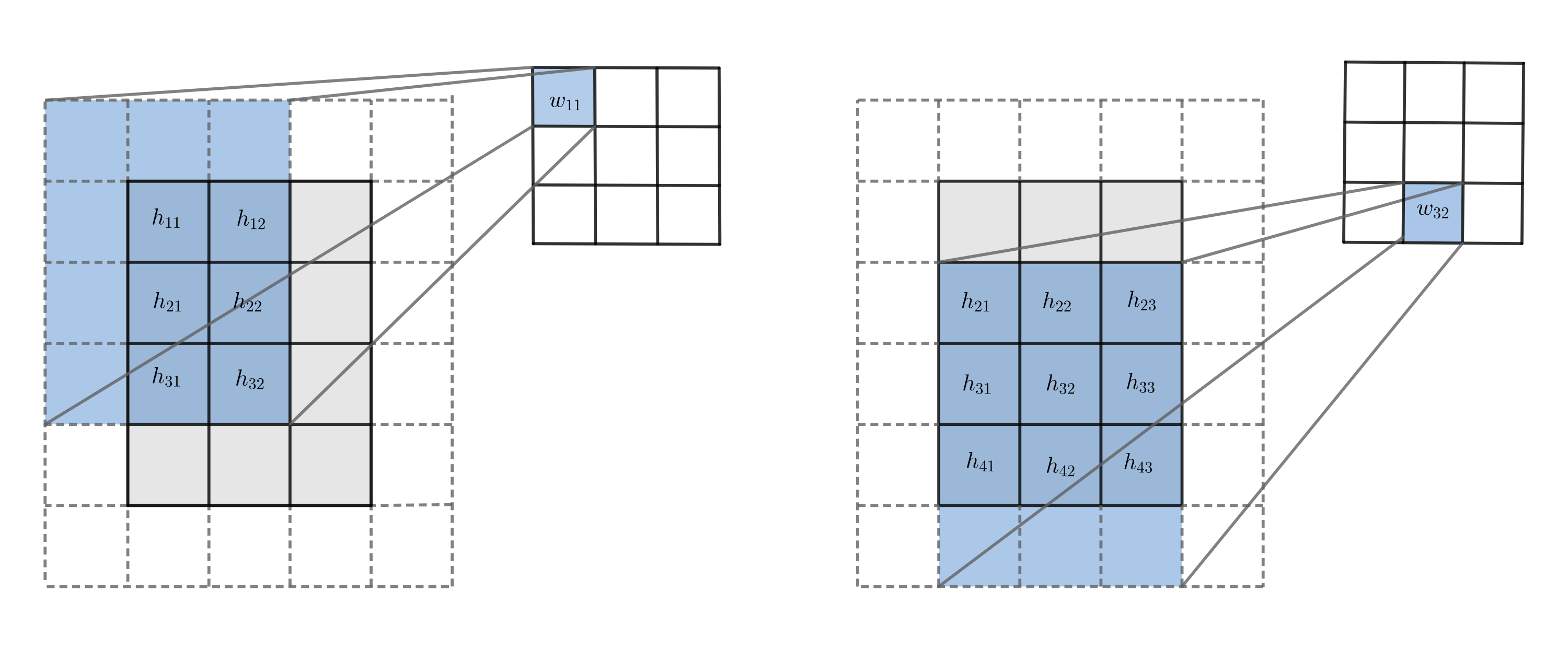
Figure 1: The blue shaded regions are $4\times 3$ submatrices in the $6\times 5$ zero padded feature matrix traced out by a single element of the kernel during convolution. Illustrated here are the cases $w_{11}$ and $w_{32}$: the entries in the submatrix make up column 1 or column 6 of $\mathcal{H}$ which correspond to $w_{11}$ or $w_{32}$, respectively.

In general, for fixed $p$ and $d$, we can write the 2-d convolution of $\mathbf{h}(\cdot,\cdot,p)$ and $\mathbf{w}(\cdot,\cdot,p,d)$ as a matrix vector product

$$\text{vec}(\text{Conv}(\mathbf{h}(\cdot,\cdot,p),\mathbf{w}(\cdot,\cdot,p,d)))=H_{p}\cdot\text{vec}(\mathbf{w}(\cdot,\cdot,p,d)),$$ (16)

where $H_{p}\in\mathbb{R}^{(rs)\times(k^{2})}$ and its $((i-1)r+u,(j-1)k+v)$ entry is the entry of the padded feature map, $\mathbf{h}(\cdot,\cdot,p)$ that is multiplied by $\mathbf{w}(j,v,p,d)$ to obtain $\mathbf{a}(u,i,d)$ in the convolution, where $1\leq u\leq r,$ $1\leq i\leq s,$ and $1\leq v,j\leq k$. As in the example above, this matrix can be written as a $s\times k$ block matrix of size $r\times k$, where the $(t,u)$ block ($1\leq t\leq s$, $1\leq u\leq k$) of $H_{p}$ is

$$(H_{p})_{tu}=\left[\begin{array}[]{cccc}\mathbf{h}(t^{\prime},u^{\prime},p)&\mathbf{h}(t^{\prime}+1,u^{\prime},p)&\ldots&\mathbf{h}(t^{\prime}+(k-1),u^{\prime},p)\\ \mathbf{h}(t^{\prime}+1,u^{\prime},p)&\mathbf{h}(t^{\prime}+2,u^{\prime},p)&\ldots&\mathbf{h}(t^{\prime}+k,u^{\prime},p)\\ \vdots&\vdots&&\vdots\\ \mathbf{h}(t^{\prime}+(r-1),u^{\prime},p)&\mathbf{h}(t^{\prime}+r,u^{\prime},p)&\ldots&\mathbf{h}(t^{\prime}+(r+k-2),u^{\prime},p)\\ \end{array}\right],$$

where $t^{\prime}=1-\frac{k-1}{2}$, $u^{\prime}=u-\frac{k-1}{2}+(t-1)$, and $\mathbf{h}(a,b,p)=0$ for any index outside its bound. In particular, the $(j-1)k+v$-th column of $H_{p}$ consists of the entries $\mathbf{h}(u,i,p)$ in the $r\times s$ submatrix of the padded feature map where the submatrix is given by $u$ and $i$ in the ranges $-\frac{k-1}{2}+1+(v-1)\leq u\leq r-\frac{k-1}{2}+(v-1)$ and $-\frac{k-1}{2}+1+(j-1)\leq i\leq s-\frac{k-1}{2}+(j-1)$.

Equation (16) allows us to relate the layer output to the input as

$$\text{vec}(\mathbf{a}(\cdot,\cdot,d)) =\sum_{p=1}^{c}\text{vec}(\text{Conv}(\mathbf{h}(\cdot,\cdot,p),\mathbf{w}(\cdot,\cdot,p,d)))+b_{d}e$$

$$=\sum_{p=1}^{c}H_{p}\cdot\text{vec}(\mathbf{w}(\cdot,\cdot,p,d))+b_{d}e$$

$$=\left[\begin{array}[]{ccccc}e&H_{1}&H_{2}&\ldots&H_{c}\end{array}\right]\cdot\widehat{w},$$

where

$$\widehat{w}=\left[\begin{array}[]{c}b_{d}\\ \omega_{d}\end{array}\right]\in{\mathbb{R}}^{ck^{2}+1}\;\mbox{ and }\;\omega_{d}=\left[\begin{array}[]{c}\text{vec}\left(\mathbf{w}(\cdot,\cdot,1,d)\right)\\ \vdots\\ \text{vec}\left(\mathbf{w}(\cdot,\cdot,c,d)\right)\end{array}\right]\in{\mathbb{R}}^{ck^{2}}.$$ (17)

Note that we use $\omega_{d}$ to denote the vector reshaping of the tensor $\mathbf{w}(\cdot,\cdot,\cdot,d)$ for a fixed $d$ and, for simplicity, we drop the dependence on $d$ in the notation of $\widehat{w}$ as $d$ is fixed for all related discussions. When training over a mini-batch of $N$ inputs, we have one $\mathbf{a}$ for each input. Combining the equations for all $N$ inputs in the mini-batch gives the linear relationship as summarized in the following lemma.

Lemma 8

Given a mini-batch of $N$ inputs, let $\{\mathbf{h}^{(1)},\cdots,\mathbf{h}^{(N)}\}$ be the associated input tensors at layer $\ell$, and $\{\mathbf{a}^{(1)},\cdots,\mathbf{a}^{(N)}\}$ the output tensors. For a fixed output channel $d$, we have $\widehat{a}=\widehat{\mathcal{H}}\cdot\widehat{w},$ where $\widehat{w}$ is defined as in (17) to be the vectorized bias and weight elements,

$${\small\widehat{\mathcal{H}}=[e,\mathcal{H}],\;\;\mathcal{H}=\left[\begin{array}[]{ccccc}H_{1}^{(1)}&\ldots&H_{c}^{(1)}\\ H_{1}^{(2)}&\ldots&H_{c}^{(2)}\\ \vdots&&\vdots\\ H_{1}^{(N)}&\ldots&H_{c}^{(N)}\\ \end{array}\right],\,\widehat{a}=\left[\begin{array}[]{c}\text{vec}\left(\mathbf{a}^{(1)}(\cdot,\cdot,d)\right)\\ \vdots\\ \text{vec}\left(\mathbf{a}^{(N)}(\cdot,\cdot,d)\right)\\ \end{array}\right],}$$ (18)

and $H_{p}^{(i)}\in{\mathbb{R}}^{rs\times k^{2}}$ is as defined in (16) from $\mathbf{h}^{(i)}$.

In the lemma, note that $\widehat{a}\in{\mathbb{R}}^{Nrs}$ and $\mathcal{H}\in{\mathbb{R}}^{Nrs\times k^{2}c}$. With this linear relationship we derive the corresponding Hessian of the loss function.

Proposition 9

Consider a CNN loss function $L$ defined for a single input tensor and write ${L}={L}(\mathbf{a}(\cdot,\cdot,d))$ as a function of the convolution kernel $\mathbf{w}(\cdot,\cdot,\cdot,d)$ through

$$\mathbf{a}(\cdot,\cdot,d){=\sum_{c=1}^{c_{l}}\text{Conv}(\mathbf{h}\left(\cdot,\cdot,c),\mathbf{w}(\cdot,\cdot,c,d)\right)}+b_{d}.$$

When training over a mini-batch with $N$ inputs, let the associated hidden variables $\mathbf{h}$ of layer $\ell$ be $\{\mathbf{h}^{(1)},\mathbf{h}^{(2)},...,\mathbf{h}^{(N)}\}$ and let the associated output of layer $\ell$ be $\{\mathbf{a}^{(1)},\mathbf{a}^{(2)},...,\mathbf{a}^{(N)}\}$. Let $\mathcal{L}=\frac{1}{N}\sum_{j=1}^{N}L(\mathbf{a}^{(j)}(\cdot,\cdot,d))$ be the mean loss over the mini-batch. Then

$$\nabla_{\widehat{w}}^{2}\mathcal{L}=\mathcal{\widehat{H}}^{T}S\mathcal{\widehat{H}},$$

where $\mathcal{\widehat{H}}$ is as defined in (18), $S=\frac{1}{N}\text{diag}\left\{\frac{\partial^{2}L}{\partial v_{a}^{2}}(v_{a}^{(1)}),\frac{\partial^{2}L}{\partial v_{a}^{2}}(v_{a}^{(2)}),\cdots,\frac{\partial^{2}L}{\partial v_{a}^{2}}(v_{a}^{(N)})\right\}$, $v_{a}:=\text{vec}(\mathbf{a}(\cdot,\cdot,d))$, and $v_{a}^{(j)}:=\text{vec}\left(\mathbf{a}^{(j)}(\cdot,\cdot,d)\right)$.

This Hessian matrix has a similar form as in the fully connected network (10). We can apply preconditioning transformation (12) to improve the conditioning of $\mathcal{\widehat{H}}$ and hence of $\nabla_{\widehat{w}}^{2}\mathcal{L}$ in the same way. As in the fully connected network, we use the preconditioner $P=UD,$ where

$$U=\begin{bmatrix}1&-\mu_{H}^{T}\\ 0&I\\ \end{bmatrix},\,\,D=\begin{bmatrix}1&0\\ 0&\text{diag}(\sigma_{H})\end{bmatrix}^{-1},$$

$\mu_{H}$ and $\sigma_{H}$ are defined from $\mathcal{H}$ as

$$\mu_{H}:=\frac{1}{Nrs}{\mathcal{H}}^{T}e=\frac{1}{Nrs}\sum_{i=1}^{Nrs}\mathcal{H}_{i},\,\;\sigma_{H}^{2}:=\frac{1}{Nrs}\sum_{i=1}^{Nrs}(\mathcal{H}_{i}-\mu_{H})^{2},$$

and $\mathcal{H}^{T}_{i}$ is the $i$th row of $\mathcal{H}$. With this $P$, $\mathcal{\widehat{H}}P$ has the same property as ${\widehat{H}}P$ for the fully connected network. By applying Theorem 4 to $\mathcal{\widehat{H}}P$, the conditioning of $\mathcal{\widehat{H}}$ is improved with the preconditioning by $P$.

Thus, the BNP transformation for a convolutional layer has the same form and the same property as in the fully connected network, except that the $\mu_{H}$ and $\sigma_{H}$ are the means and variances over the columns of $\mathcal{H}$. Noting that each column of $\mathcal{H}$ contains the elements of the feature maps that are multiplied by the corresponding kernel entry during the convolution for all inputs in a mini-batch, thus the means and variances are really the means and variances over the $N$ submatrices of feature maps defined by the kernel convolution for the mini-batch. See Figure 1 for a depiction. Mathematically, we can express the $(p-1)k^{2}+(a-1)k+t$ entry of vector mean $\mu_{H}$ and vector variance $\sigma_{H}$ corresponding to ${\bf w}(t,a,p,d)$, indexed by $(t,a,p)$, as

$$\mu_{H}(t,a,p)=\frac{1}{Nrs}\sum_{i=1}^{N}\sum_{u=t-\frac{k-1}{2}}^{r+t-\frac{k-1}{2}-1}\sum_{v=a-\frac{k-1}{2}}^{s+a-\frac{k-1}{2}-1}h^{(i)}(u,v,p)$$ (19)

and

$$\sigma_{H}^{2}(t,a,p)=\frac{1}{Nrs}\sum_{i=1}^{N}\sum_{u=t-\frac{k-1}{2}}^{r+t-\frac{k-1}{2}-1}\sum_{v=a-\frac{k-1}{2}}^{s+a-\frac{k-1}{2}-1}(h^{(i)}(u,v,p)-\mu(t,a,p))^{2},$$ (20)

for $1\leq t,a\leq k$ and $1\leq p\leq c$.

The entries in $\mu_{H}$ and $\sigma^{2}_{H}$ vary slightly from entry to entry, being the means and variances of different submatrices of the zero-padded feature maps used, which mostly overlap with the feature map. If $r,s$ are large, they are all approximately equal to the mean and variance of the feature map $\mathbf{h}(\cdot,\cdot,p)$ over the mini-batch for each fixed input channel $p$, written as

$${\mu(p)=\frac{1}{Nrs}\sum_{i=1}^{N}\sum_{u=1}^{r}\sum_{v=1}^{s}h^{(i)}(u,v,p)}$$ (21)

and

$${\sigma(p)^{2}=\frac{1}{Nrs}\sum_{i=1}^{N}\sum_{u=1}^{r}\sum_{v=1}^{s}(h^{(i)}(u,v,p)-\mu)^{2}},$$ (22)

where $\mu$ and $\sigma$ are vectors with $\mu(p)$ and $\sigma(p)$ as entries. Using this approximation significantly saves computations, which is adopted in our implementation of BNP. Indeed, this is how BN normalizes the activation of a convolution layer in CNNs.

The error in approximating $\mu_{H}(i,j,p)$ and $\sigma_{H}(i,j,p)$ for all $i,j$ by $\mu(p)$ and $\sigma(p)$ is given by the difference between the feature maps and the submatrices of the padded feature maps. They have the same dimension and differ at most in $\frac{k-1}{2}$ columns and rows on the border of the feature map, replacing these border entries with the zeros of the padded feature map; see Figure 2 for an illustration. The error can be bounded as in the following proposition, which shows that, if the feature map size, $r,s$, is much bigger than the kernel size $k$, the error is small.

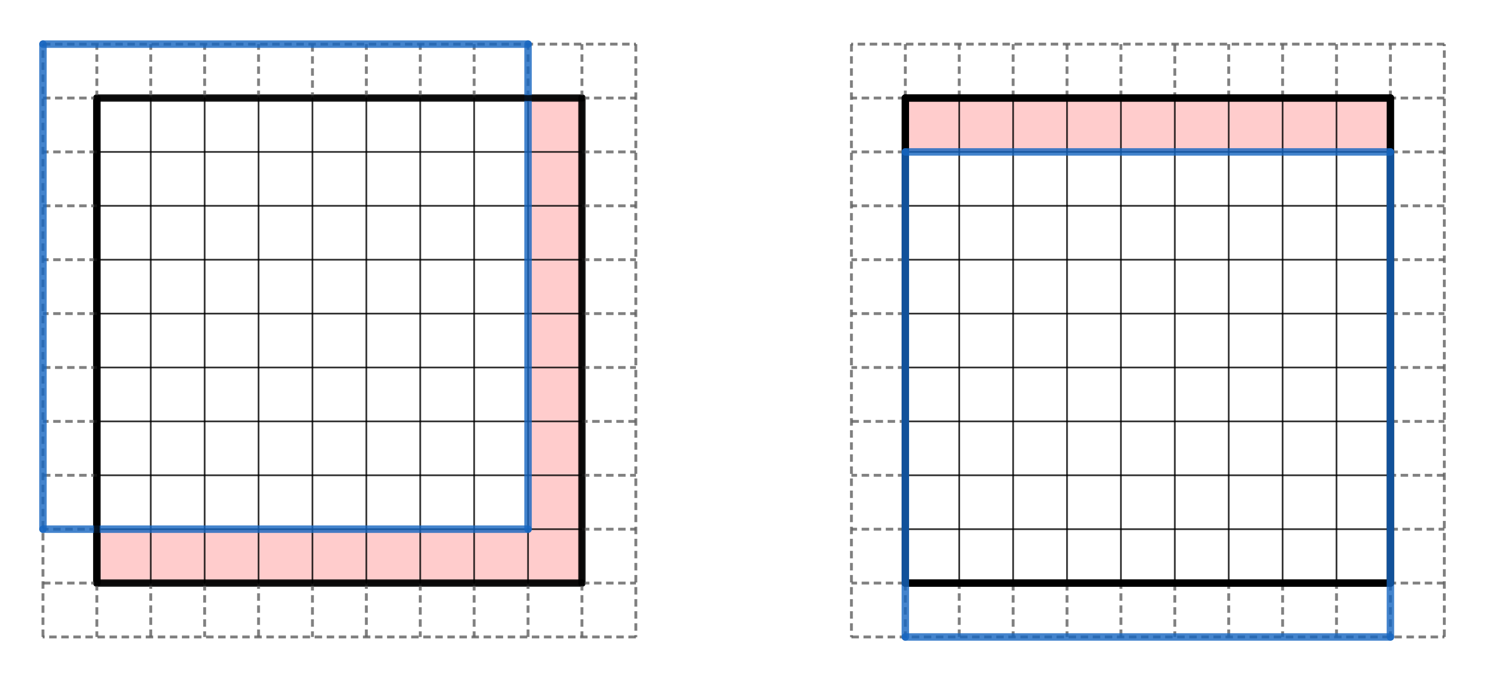
Figure 2: The $9\times 9$ blue submatrix of the zero padded feature map consists of the elements traced out by $w_{11}$ (Left) or $w_{32}$ (Right) in the $3\times 3$ kernel convolution. The mean $\mu_{H}$ and variance $\sigma_{H}$ are taken over these blue submatrices, while $\mu$ and $\sigma$ are taken over the $9\times 9$ feature map, outlined in bold. The error in our approximation is given by the difference in elements, in shaded red above; those elements of the feature map excluded from the submatrix. There is a difference of at most $\frac{k-1}{2}$ rows and columns on the border of the feature map. Thus for $r,s\gg k$, this error is small.

Proposition 10

Under the notation defined in Proposition 9, the error $|\mu(t,a,p)-\mu(p)|$ of approximating $\mu(t,a,p)$, the mean calculated for the BNP transformation, as defined in (19), by $\mu(p)$, as in (21), the mean over the entire feature map, is bounded by

$${(k-1)\left(\frac{1}{2r}+\frac{1}{2s}-\frac{k-1}{4rs}\right)\max_{u,v,i}{|h^{(i)}(u,v,p)|}}.$$

As in Section 3.3, we further consider scaling each Hessian block to have comparable norms by estimating the norm of $\mathcal{H}$. A direct application of Proposition 5 to $\mathcal{\widehat{H}}P$ would indicate a norm bounded by $\max\{\sqrt{k^{2}c},\sqrt{Nrs}\}$, where $k^{2}c$ is the number of its columns and $Nrs$ is the number of its rows. But one difficulty is that $\mathcal{H}$ contains many shared entries, so the entries of $\mathcal{\widehat{H}}P$ can no longer be modeled as independent random variables. We note that $\mathcal{H}$ in (18) has $N$ block rows where each block entry $H_{p}^{(i)}$ has $rs$ rows, but its columns are rearrangements of mostly the same entries. Namely, the entire matrix $H_{p}^{(i)}$ contains only $rs$ independent entries. Thus, it may be effectively considered a matrix of independent entries with $\sqrt{rs}$ rows. Then $\mathcal{\widehat{H}}P$ may be regarded as having effectively $N\sqrt{rs}$ rows. We therefore suggest to use $\max\{\sqrt{k^{2}c},\sqrt{N}(rs)^{1/4}\}$ as a norm estimate. Thus, we scale $\mathcal{\widehat{H}}P$ by $q$, i.e. use $(1/q)P$ as a preconditioner, where $q^{2}=\text{max}\{{k^{2}c/N},\sqrt{rs}\}$. Our experiments with several variations of CNNs shows that this heuristic based estimate works well.

The detailed BNP preconditioning transformation for the $\ell$th convolution layer with the wight tensor ${\bf w}$ and bias vector $b$ (with their dependence on $\ell$ dropped in the notation for simplicity) is carried out in the vector reshaped from the tensor. Let $W=\begin{bmatrix}\omega_{1},...,\,\omega_{c_{\ell}}\end{bmatrix}\in\mathbb{R}^{k^{2}c_{\ell-1}\times c_{\ell}}$ be the matrix representation of ${\bf w}$ where the first three dimensions are reshaped into a vector, i.e. $\omega_{d}=vec({\bf w}(\cdot,\cdot,\cdot,d))$ (see (17)). Let $\mu\in\mathbb{R}^{c_{\ell-1}}$ and $\sigma\in{\mathbb{R}}^{c_{\ell-1}}$ be defined in (21) and (22), e.g. $\mu=\begin{bmatrix}\mu(1),\,.\,.\,.,\,\mu(c_{\ell-1})\end{bmatrix}^{T}\in\mathbb{R}^{c_{\ell-1}}$. Then $\mu_{H}$ and $\sigma_{H}$ are approximated by $\mu\otimes e:=\begin{bmatrix}\mu(1)e^{T},\,.\,.\,.,\,\mu(c_{\ell-1})e^{T}\end{bmatrix}^{T}\in\mathbb{R}^{k^{2}c_{\ell-1}}$ and $\sigma\otimes e:=\begin{bmatrix}\sigma(1)e^{T},\,.\,.\,.,\,\sigma(c_{\ell-1})e^{T}\end{bmatrix}^{T}\in\mathbb{R}^{k^{2}c_{\ell-1}}$, and $e=[1,1,\cdots,1]^{T}\in\mathbb{R}^{k^{2}}$. Then, the preconditioned gradient descent is the following update in $W$ and $b$:

$$\begin{bmatrix}b^{T}\\ W\end{bmatrix}\leftarrow\begin{bmatrix}b^{T}\\ W\end{bmatrix}-\alpha\frac{1}{q^{2}}PP^{T}\begin{bmatrix}\frac{\partial\mathcal{L}}{\partial b}\\ \frac{\partial\mathcal{L}}{\partial W}\end{bmatrix};\;\;P=\begin{bmatrix}1&-\mu^{T}\otimes e^{T}\\ 0&I\end{bmatrix}\begin{bmatrix}1&0\\ 0&\text{diag}\left(\frac{1}{{\tilde{\sigma}\otimes e}}\right)\end{bmatrix},$$ (23)

This vector form of the gradient descent update can be stated in the original tensor ${\bf w}$ with the matrix multiplications by $P$ and $P^{T}$ simplified. We present it in Algorithm 3.

Algorithm 3 One Step of BNP Training of a Convolution Layer with weight ${\bf w}$ and bias $b$

Given: $\epsilon_{1}=10^{-2},\epsilon_{2}=10^{-4}$ and $\rho=0.99$; learning rate $\alpha$;

initialization: $\mu=0,\sigma=1$;

Input: Mini-batch output of previous layer $H=[h_{1}^{(\ell-1)},h_{2}^{(\ell-1)},\ldots,h_{N}^{(\ell-1)}]^{T}\subset\mathbb{R}^{c_{\ell-1}\times r\times s}$ and the parameter gradients: $G_{\mathbf{w}}\leftarrow\frac{\partial\mathcal{L}}{\partial\mathbf{w}}\in\mathbb{R}^{k\times k\times c_{\ell-1}\times c_{\ell}};G_{b}\leftarrow\frac{\partial\mathcal{L}}{\partial b}\in\mathbb{R}^{1\times c_{\ell}}$

1. Compute mini-batch mean/variance: $\hat{\mu},\hat{\sigma}^{2}\in\mathbb{R}^{c_{\ell-1}}$ according to (21) and (22);

2. Compute running statistics: $\mu\leftarrow\rho\mu+(1-\rho)\hat{\mu}$, $\sigma^{2}\leftarrow\rho\sigma^{2}+(1-\rho)\hat{\sigma}^{2}$;

3. Set $\tilde{\sigma}^{2}=\sigma^{2}+\epsilon_{1}\max\{\sigma^{2}\}+\epsilon_{2}$ and $q^{2}=\text{max}\{c_{\ell-1}k^{2}/N,\sqrt{rs}\}$;

4. Update $G_{\mathbf{w}}$: $G_{\mathbf{w}}(i,j,p,d)\leftarrow\frac{1}{q^{2}}\left(G_{\mathbf{w}}(i,j,p,d)-\mu(p)G_{b}(d)\right)/\tilde{\sigma}(p)^{2}$;

5. Update $G_{b}$: $G_{b}(d)\leftarrow\frac{1}{q^{2}}G_{b}(d)-\sum_{i,j,p}\mu(p)G_{\mathbf{w}}(i,j,p,d)$;

Output: updated gradients: $G_{\mathbf{w}},G_{b}$

Finally, we remark that our derivation of preconditioning $\mathcal{\widehat{H}}$ leads to the normalization by mean and variance over the mini-batch and the two spatial dimensions. This not only provides a justification to the conventional approach in applying BN to CNNs but also validates our theory. Note that a straightforward application of BN to CNNs may suggest normalizing each pixel by the pixel mean and variance over a mini-batch only. Under our theory, it is the Hessian matrix of Proposition 9 that determines what mean and variance should be used in normalization. In particular, the means and variances of the columns of $\mathcal{\widehat{H}}$, the extended hidden variable matrix, naturally lead to the corresponding definitions.

Another interesting implication of our theory concerns online learning with mini-batch size $N=1$. Unlike BN, BNP is not constrained on the mini-batch size. For the fully connected network, however, $\widehat{H}$ in (11) has 1 row only and hence a condition number of 1, which can not be reduced. So, although BNP may still be beneficial due to Hessian block norm balancing, the effect is not expected to be as significant as with larger $N$. However, for CNNs, $\mathcal{\widehat{H}}$ has dimension $Nrs\times(k^{2}c+1)$ and even when $N=1$ the preconditioning can still offer improvements by Theorem 4.

5 Experiments

In this section, we compare BNP with several baseline methods on several architectures for image classification tasks. We also present some exploratory experiments to study computational timing comparison as well as improved condition numbers.

First, we present experiments comparing BNP with BN (and Batch Renorm when a small mini-batch size is used) and vanilla networks. Where suitable, we also compare with LayerNorm (LN) and GroupNorm (GN) as well as a version of BN with 4 things/improvements (Summers and Dinneen, 2020). We test them in three architectures for image classification: fully connected networks, CNNs, and ResNets. All models use ReLU nonlinearities and the cross-entropy loss. Each model is tuned with respect to the learning rate. Default hyperparameters for BN and optimizers as implemented in Tensorflow or PyTorch are used, as appropriate. For BNP, the default values $\epsilon_{1}=10^{-2}$, $\epsilon_{2}=10^{-4}$, and $\rho=0.99$ are also used. Other detailed experimental settings are given in Appendix B.

Data sets: We use MNIST, CIFAR10, CIFAR100, and ImageNet data sets. The MNIST data set (LeCun et al., 2013) consists of 70,000 black and white images of handwritten digits ranging from 0 to 9. Each image is 28 by 28 pixels. There are 60,000 training images and 10,000 testing images. The CIFAR10 and CIFAR100 data sets (Krizhevsky et al., 2009) consist of 60,000 color images of 32 by 32 pixels with 50,000 training images and 10,000 testing images. The CIFAR10 and CIFAR100 data sets consist of 10 and 100 classes respectively. The ImageNet datatset (Russakovsky et al., 2015) consists of 1,431,167 color images with 1,281,167 training images, 50,000 validation images, and 100,000 testing images. Each image has 256 by 256 pixels and the ImageNet dataset consists of 1,000 classes.

Fully Connected Neural Network. We follow Ioffe and Szegedy (2015) and consider a fully connected network consisting of three hidden layers of size 100 each and an output layer of size 10. We test it on the MNIST and CIFAR10 data sets. For each experiment, we flatten each image into one large vector as input. For the BN networks, normalization is applied post-activation. For this experiment, we also compare against an additional baseline of LayerNorm (LN), which is not affected by small batch size. Each model is trained using SGD.

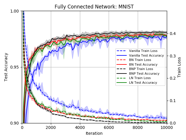
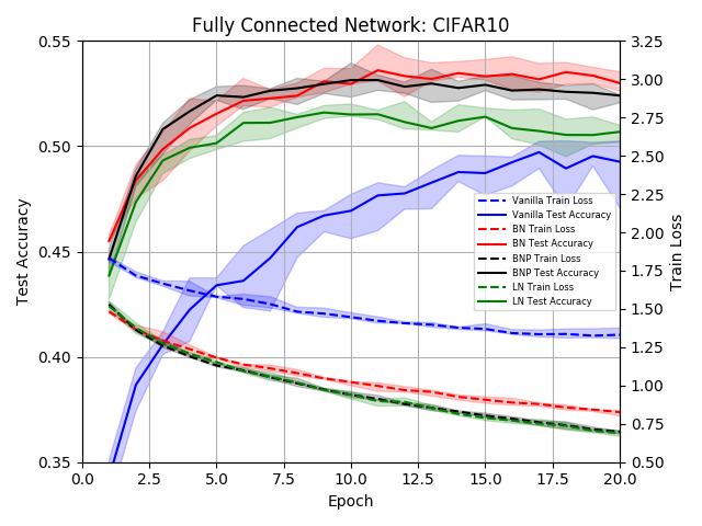
Figure 3: Fully connected network with mini-batch size 60: Training loss (dashed lines) and test accuracy (solid lines) for the vanilla network, BN, LN, and BNP on MNIST (Left) and CIFAR10 (Right). The lines graph the means while the shaded regions graph the ranges of 5 tests.

We first test on MNIST and CIFAR10 with mini-batch size 60, and the results, averaged over 5 runs with the mean and the range, are plotted in Figure 3. BN and BNP have comparable performance in the MNIST experiments, with BN slightly faster at the beginning and BNP outperforming after that. They slightly outperform LN and all improve over the vanila network. For the CIFAR10 experiment, we see that BNP and BN are also comparible, with BNP converging slightly faster at the beginning but mildly overfitting after the 10th epoch, while BN achieving slightly better final accuracy without any overfitting. In both cases, BNP and BN outperform the vanilla and LN networks. In general, BN does well in large mini-batch sizes and is less likely to overfit.

We also consider small mini-batch sizes and present the averaged results with mini-batch sizes 6 and 1 for CIFAR10 in Figure 4. With mini-batch size 6, BNP outperforms BN and the vanilla network. This demonstrates how small mini-batch sizes can negatively affect BN. We also compare with Batch Renorm and LN in this test. Batch Renorm and LN perform better than BN and are more comparable to BNP, where BNP converges slightly faster but Batch Renorm achieves the same final accuracy. For mini-batch size 1, BN and BN Renorm do not train and are not included in the plot. BNP, LN and the vanilla network all train with mini-batch size 1. BNP and LN converges significantly faster than the vanilla network. They overfit very slightly to have final test accuracy trending just below the vanilla network.

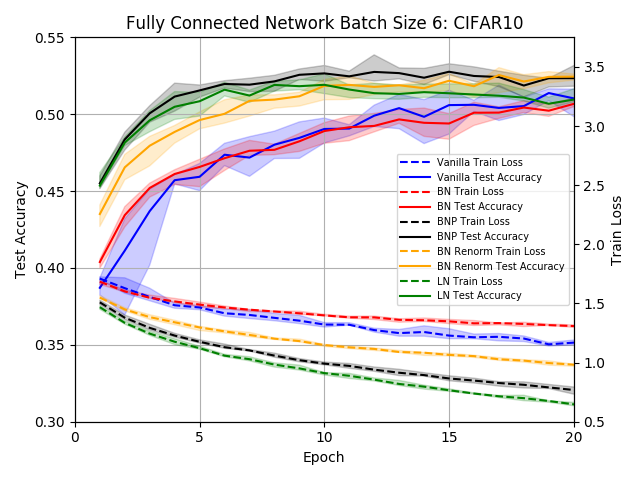
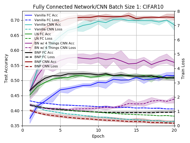
Figure 4: Fully connected (FC) network/CNN with small mini-batch sizes (6 and 1): Training loss (dashed lines) and test accuracy (solid lines). Left: fully connected network with mini-batch size 6 for vanilla network, BN, BN Renorm, LN, and BNP; Right: fully connected (FC) network and 5-layer CNN with mini-batch size 1 for vanilla network, LN or BN w/ 4 Things, and BNP. BN and BN Renorm do not train and their results are not plotted. The lines graph the means while the shaded regions graph the ranges of 5 tests.

Convolutional Neural Networks. We consider a 5-layer CNN as used in TensorFlow (2019). This network consists of 3 convolution layers, each with a $3\times 3$ kernel, of filter size $32$-$64$-$32$, followed by two dense layers. For this experiment, we also include the version of BN with 4 things/improvements (Summers and Dinneen, 2020). These improvements are as follows: for small batch size, BN is combined with GN, while for larger batch-sizes BN is combined with Ghost Normalization; additionally a weight decay regularization on BN’s $\gamma,\beta$ terms and a method to incorporate example statistics during inference are applied (Summers and Dinneen, 2020). In particular, the combination with GN makes it applicable to mini-batch size 1.

We use SGD with the exception of the vanilla and the BN with 4 Things networks where Adam performs better and was used. Figure 5 presents the results with 5 tests for CIFAR10 with mini-batch sizes 128 and 2. For mini-batch size 128, we find that BN, BN with 4 Things, and BNP all have comparable performance with BNP converging slightly slower and BN with 4 Things slightly faster than BN at the beginning. They all outperform the vanilla network. For mini-batch size 2, BNP significantly outperforms BN, Batch Renorm, and BN with 4 Things. BN underperforms all other methods. However, we note that BN and Batch Renorm work well for batch sizes as small as 4 and 3 respectively. Compared with the fully connected network, BN appears to be effective in CNNs for much smaller mini-batch size.

We also test on mini-batch size 1 with 5 test results given in Figure 4 (Right). As expected, BN and BN Renorm do not train and their results are not included in the figure. BNP trains faster and reaches slightly higher accuracy than the vanilla network, while BN with 4 Things significantly underperforms with mini-batch size 1.

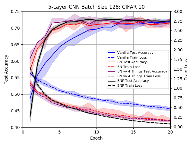
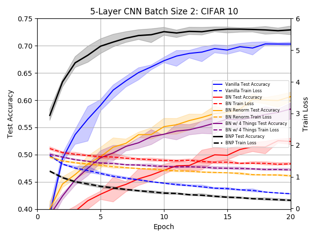
Figure 5: 5-layer CNN for mini-batch size 128 (Left) and mini-batch size 2 (Right): Training loss (dashed lines) and test accuracy (solid lines) for vanilla network, BN, BN w/ 4 Things, and BNP. For batch-size 2, BN Renorm is also included. The lines graph the means while the shaded regions graph the ranges of 5 tests.

Our results demonstrate that BNP works well in the setting of small mini-batch sizes or the online setting. In this situation, it can significantly outperform BN for both fully connected networks and CNNs. It also produces comparable results when larger mini-batch sizes are used.

Residual Networks. We consider 110-layer Residual Networks (ResNet-110) (He et al., 2016a, b), and an 18-layer Residual Network (ResNet-18). The ResNet-110 has 54 residual blocks, containing two $3\times 3$ convolution layers each block and was used for CIFAR 10/CIFAR 100 (He et al., 2016a, b). We experiment with both the original ResNet-110 (He et al., 2016a) and its preactivation version (He et al., 2016b). The ResNet-18 has 8 residual blocks, with two $3\times 3$ convolution layers each block and was used for ImageNet (He et al., 2016a). We follow the settings of (He et al., 2016a, b) by using the data augmentation as in He et al. (2016a), the momentum optimizer, learning rate decay, learning rate warmup, and weight decay; see Appendix B for details. In particular, we use learning rate decay at epoch 80/120 (CIFAR10), epoch 150/220 (CIFAR100), and epoch 30/60/90 (ImageNet).

One remarkable property of BN when applied to ResNet is its significant increase in test accuracy at learning rate decay. Like most other methods, BNP directly applied to ResNet can not take advantage of the learning rate decay nearly to the same degree as BN, even though BNP converges faster before the learning rate decay; see Figure 6. We suspect this is due to the lack of scale-invariant property in BNP that is present in BN. Since GN also possess the scale-invariant property, we may combine BNP with GN; see Section 3.5. So, for the ResNet experiment, we apply BNP to ResNet with GN, denoted by BNP+GN, which is found to benefit much more significantly from learning rate decay. For comparison, we also include ResNet with GN in this experiment.

We test ResNet-110 on CIFAR10 and present the results of 5 runs in Figure 6 (Left). The test accuracy for BNP+GN converges faster than BN prior to the first learning rate decay at the 80th epoch and is comparable to BN after the decay. Both BNP+GN and BN outperform GN significantly.

We then test preactivation ResNet-110 on CIFAR100 and present the results of 5 runs in Figure 6 (Right). The test accuracy for BNP+GN also converges faster than BN prior to the first learning rate decay at the 150th epoch but is slightly lower than BN after the decay. Both BNP+GN and BN outperform GN significantly.

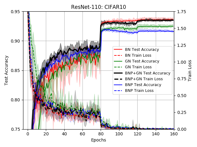
Figure 6: ResNet-110 for CIFAR10 (Left) and Preactivation ResNet-110 for CIFAR100 (Right): Training loss (dashed lines) and test accuracy (solid lines) for BN, GN, BNP alone, and BNP+GN. Both with mini-batch size 128. The lines graph the means while the shaded regions graph the ranges of 5 tests.

We lastly test ResNet-18 on ImageNet and present the results in Figure 7. The test accuracy for BNP+GN again converges faster than BN prior to the first learning rate decay at the 30th epoch but is slightly lower than BN after the second decay at the 60th. Again, BNP+GN and BN outperform GN significantly.

We observe that, for all three ResNets, BNP with the help of GN achieves faster convergence before learning rate decay, while producing comparable final accuracy at the end. With GN’s performance lagging, these results can be attributed to BNP and demonstrates the convergence acceleration property of BNP.

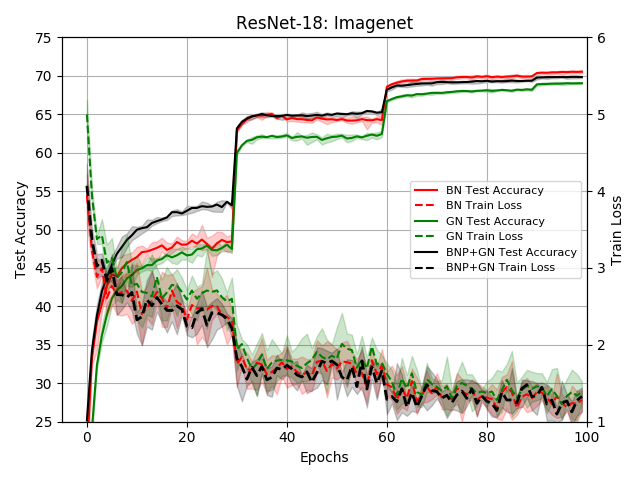
Figure 7: ResNet-18 for ImageNet: Training loss (dashed lines) and test accuracy (solid lines) for BN, GN, and BNP+GN. All have mini-batch size 256.

5.1 Exploratory Experiments

We present experiments that support our theory that BNP lowers the condition number of the Hessian of the loss function in relation to the condition number of matrix $D$ used in the preconditioning transformation as detailed in Section 3. We also present a computational timing comparison between BN and BNP.

Condition Number Analysis: We consider a fully connected network consisting of two hidden layers of size 100 and an output layer of size 10. We use the CIFAR10 data set with mini-batch size 60. With this network we compute the condition number of the Hessian with respect to a single weight vector and bias entry at each iteration. In particular, we consider the first weight vector and bias entry in the output layer, that is $\hat{w}^{T}=[b_{3}^{(1)},w_{3}^{(1)}]\in\mathbb{R}^{1\times 101}$, and compute the condition number of the Hessian of the loss function with respect to $\hat{w}$. Results for this condition number and the one for the preconditioned Hessian are given in Figure 8 (Center). The preconditioning significantly reduces the condition number of the Hessian. For this same layer, we compute the condition number of matrix $D$. Note that, when $D$ is ill-conditioned, that is when the variances of the activations differ in magnitude, we expect the preconditioning transformation to improve the condition number of the Hessian by approximately $\kappa(D)^{2}$. For this small network, Figure 8 (Right) shows the condition number of $D$ to be in the range $10^{2}-10^{5}$. As a result, the BNP transformation reduces the condition number by roughly $\kappa(D)^{2}$. We also graph test accuracy and training loss of our Vanilla network versus BNP which confirms accelerated convergence by BNP. These results support our theory.

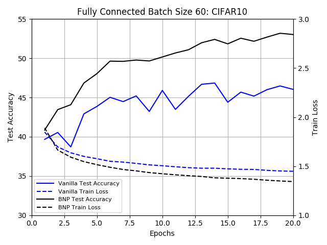
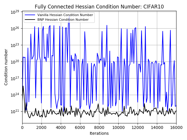
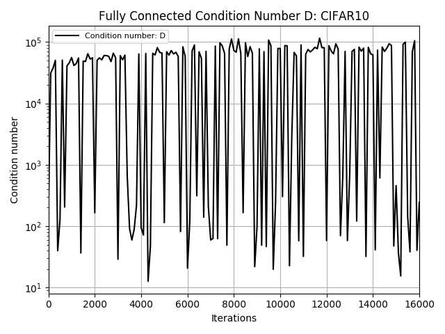
Figure 8: We compare the test accuracy (solid lines) and training loss (dashed lines) of a vanilla network with BNP (Left). With this same network we graph and compare the condition number of the Hessian and the preconditioned Hessian by BNP (Center) as well as the condition number of matrix $D$, used in the preconditioning transformation (Right).

Computation Time Analysis: We include experiments on the performance time of BN versus BNP over each training epoch. We use the same fully connected network as described in the condition number experiments. These performance time experiments are computed on NVIDIA Tesla V100-SXM2-32GB. We compute the time over each epoch of training and report the cumulative training time over 20 epochs as seen in Figure 9. We also report the average time to complete one epoch of training with the respective mini-batch sizes in Table 1. We find that for smaller mini-batch size BN is faster than BNP and for larger mini-batch size BNP has a tiny improvement over BN. Overall, the difference is small and the two methods are quite comparable in computational efficiency.

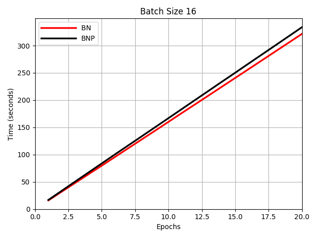
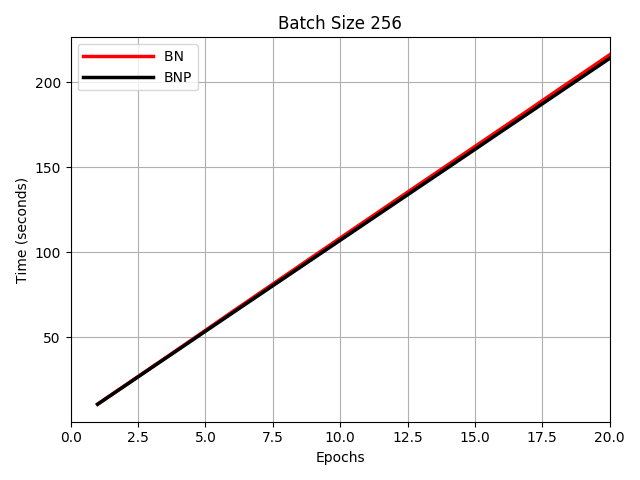
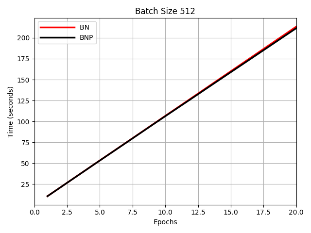
Figure 9: Time analysis comparison of BN with BNP. We compare mini-batch sizes of 16, 256, and 512 shown respectively above.

Average Computed Time Over One Epoch
	mini-batch size 16	mini-batch size 256	mini-batch size 512
BN	16.08	10.81	10.67
BNP	16.69	10.70	10.57

Table 1: Above we report the average time (in seconds) to complete one training epoch in our small fully connected network given mini-batch sizes 16, 256, and 512.

6 Conclusion

We have introduced the BNP algorithm that increases the convergence rate of training. This is done by an implicit change of variables through preconditioned gradient descent. The BNP algorithm is explicitly derived and theoretically supported. It is shown to be equivalent to BN over one training iteration if the back-propagation does not pass through the mini-batch statistics. Its flexibility in using approximate batch statistics allows it to work with small mini-batch sizes. To summarize the contributions of this work, our theory provides an insight on why BN works and how it should be applied to CNNs, and our algorithm provides a practical alternative to BN when a very small mini-batch size is used.

Acknowledgments

This research was supported in part by NSF under the grants DMS-1620082 and DMS-1821144. We would like to thank three anonymous referees for many constructive comments and suggestions that have significantly improved the paper. We would also like to thank the University of Kentucky Center for Computational Sciences and Information Technology Services Research Computing for their support and use of the Lipscomb Compute Cluster and associated research computing resources.

Appendix A. Proof of Theorems

In this appendix, we present the proofs of theorems not proven in the discussions of the main text. In particular, Theorem 3, Proposition 6, and Lemma 8 are omitted for this reason. For all remaining proofs, we restate the original theorems for completeness.

Theorem 1 Consider a loss function $\mathcal{L}$ with continuous third order derivatives and with a positively scale-invariant property. If $\theta=\theta^{*}(t)$ is a positively scale-invariant manifold at local minimizer $\theta^{*}$, then the null space of the Hessian $\nabla^{2}\mathcal{L}(\theta^{*}(t))$ contains at least the column space ${\rm Col}\left(D_{t}\theta^{*}(t)\right)$. Furthermore, for the gradient descent iteration $\theta_{k+1}=\theta_{k}-\alpha\nabla\mathcal{L}(\theta_{k})$, let $\theta^{*}_{k}$ be the local minimizer closest to $\theta_{k}$, i.e. $\theta^{*}_{k}=\theta^{*}(t_{k})$ where $t_{k}=\text{argmin}_{t>0}\|\theta_{k}-\theta^{*}(t)\|$ and assume that the null space of $\nabla^{2}\mathcal{L}(\theta^{*}(t))$ is equal to ${\rm Col}\left(D_{t}\theta^{*}(t)\right)$. Then, for any $\epsilon>0$, if our initial approximation $\theta_{0}$ is such that $||\theta_{0}-\theta^{*}_{0}||$ is sufficiently small, then we have, for all $k\geq 0$,

$$||\theta_{k+1}-\theta^{*}_{k+1}||\leq(r+\epsilon)||\theta_{k}-\theta^{*}_{k}||,$$

where $r=\max\{|1-\alpha\lambda^{*}_{min}|,||1-\alpha\lambda_{max}||\}$ and $\lambda^{*}_{min}$ and $\lambda_{max}$ are the smallest nonzero eigenvalue and the largest eigenvalue of $\nabla^{2}\mathcal{L}(\theta^{*}_{k})$, respectively.

Proof  The proof of the first part is contained in §3.2. Here we prove the second part.

Since $\theta^{*}_{k}=\theta^{*}(t_{k})$ is the local minimizer closest to $\theta_{k}$, i.e. $\|\theta_{k}-\theta^{*}(t_{k})\|=\min_{t}\|\theta_{k}-\theta^{*}(t)\|$, taking derivation in $t$ results in $(\theta_{k}-\theta^{*}(t_{k}))^{T}D_{t}\theta^{*}(t_{k})=0$. Then $(\theta_{k}-\theta^{*}_{k})$ is perpendicular to the null space of the Hessian. Furthermore, $||\theta_{k+1}-\theta^{*}_{k+1}||\leq||\theta_{k+1}-\theta^{*}_{k}||$.

Using $\theta_{k+1}=\theta_{k}-\alpha\nabla\mathcal{L}(\theta_{k})$, we have

$$||\theta_{k+1}-\theta^{*}_{k+1}|| \leq||\theta_{k+1}-\theta^{*}_{k}||$$

$$=||\theta_{k}-\alpha\nabla\mathcal{L}(\theta_{k})-\theta^{*}_{k}||$$

$$=||\theta_{k}-\theta^{*}_{k}-\alpha(\nabla\mathcal{L}(\theta_{k})-\nabla\mathcal{L}(\theta^{*}_{k}))||$$ (24)

Since $\mathcal{L}$ has continuous third order derivatives, we have $\nabla\mathcal{L}(\theta_{k})=\nabla\mathcal{L}(\theta^{*}_{k})+\nabla^{2}\mathcal{L}(\theta^{*}_{k})(\theta_{k}-\theta^{*}_{k})+e_{k}$, where $e_{k}$ is the remainder with $||e_{k}||\leq C||\theta_{k}-\theta^{*}_{k}||^{2}$ for some $C$. Substituting into Equation (24), we get

$$||\theta_{k+1}-\theta^{*}_{k+1}|| \leq||\theta_{k}-\theta^{*}_{k}-\alpha\nabla^{2}\mathcal{L}(\theta^{*}_{k})(\theta_{k}-\theta^{*}_{k})||+\alpha||e_{k}||$$

$$=||(I-\alpha\nabla^{2}\mathcal{L}(\theta^{*}_{k}))(\theta_{k}-\theta^{*}_{k})||+\alpha||e_{k}||$$ (25)

$$\leq\max_{\lambda_{i}\neq 0}|1-\alpha\lambda_{i}|\cdot||\theta_{k}-\theta^{*}_{k}||+\alpha C||\theta_{k}-\theta^{*}_{k}||^{2},$$

where $\lambda_{1},...,\lambda_{n}$ are eigenvalues of $\nabla^{2}\mathcal{L}(\theta^{*}_{k})$ and we have used that $\theta_{k}-\theta^{*}_{k}$ is perpendicular to the null space in the last inequality. Notice

$$\max_{\lambda_{i}\neq 0}|1-\alpha\lambda_{i}|=\max\{|1-\alpha\lambda^{*}_{\min}|,|1-\alpha\lambda_{\max}|\}=r.$$

We have

$$||\theta_{k+1}-\theta^{*}_{k+1}||\leq r\cdot||\theta_{k}-\theta^{*}_{k}||+\alpha C||\theta_{k}-\theta^{*}_{k}||^{2}=\big{(}r+\alpha C||\theta_{k}-\theta^{*}_{k}||\big{)}\cdot||\theta_{k}-\theta^{*}_{k}||.$$ (26)

Clearly, $r<1$. For any $\epsilon>0$ with $r+\epsilon\leq 1$, let $\delta=\frac{\epsilon}{\alpha C}$. Then, if $||\theta_{k}-\theta^{*}_{k}||<\delta$, we have

$$||\theta_{k+1}-\theta^{*}_{k+1}||\leq\big{(}r+\alpha C\delta\big{)}\cdot||\theta_{k}-\theta^{*}_{k}||\leq||\theta_{k}-\theta^{*}_{k}||<\delta.$$

Thus, if $||\theta_{0}-\theta^{*}_{0}||<\delta,$ by an induction argument, we have $||\theta_{k}-\theta^{*}_{k}||<\delta$ for all $k$. Hence,

$$||\theta_{k+1}-\theta^{*}_{k+1}||\leq(r+\epsilon)||\theta_{k}-\theta^{*}_{k}||.$$

 

Proposition 2. Consider a loss function $L$ defined from the output of a fully connected multi-layer neural network for a single network input $x$. Consider the weight and bias parameters $w_{i}^{(\ell)},b_{i}^{(\ell)}$ at the $\ell$-layer and write $L=L\left(a_{i}^{(\ell)}\right)=L\left(\widehat{w}^{T}\widehat{h}\right)$ as a function of the parameter $\widehat{w}$ through $a_{i}^{(\ell)}$ as in (9). When training over a mini-batch of $N$ inputs, let $\{h_{1}^{(\ell-1)},h_{2}^{(\ell-1)},\ldots,h_{N}^{(\ell-1)}\}$ be the associated $h^{(\ell-1)}$ and let $\widehat{h}_{j}=\begin{bmatrix}1\\ h_{j}^{(\ell-1)}\end{bmatrix}\in\mathbb{R}^{(n_{\ell}+1)\times 1}$. Let

$$\mathcal{L}=\mathcal{L}(\widehat{w}):=\frac{1}{N}\sum_{j=1}^{N}L\left(\widehat{w}^{T}\widehat{h}_{j}\right)$$

be the mean loss over the mini-batch. Then, its Hessian with respect to $\hat{w}$ is

$$\nabla^{2}_{\widehat{w}}\mathcal{L}(\widehat{w})=\widehat{H}^{T}S\widehat{H}$$

where

$$\widehat{H}=[e,\;H],{H}=\begin{bmatrix}h_{1}^{(\ell-1)^{T}}\\ \vdots\\ h_{N}^{(\ell-1)^{T}}\end{bmatrix}\text{ and }S=\frac{1}{N}\text{diag}\left(L^{\prime\prime}\left(\widehat{w}^{T}\widehat{h}_{j}\right)\right).$$

with all off-diagonal elements of $S$ equal to 0.

Proof  First, we have $\nabla_{\widehat{w}}L\left(\widehat{w}^{T}\widehat{h}\right)=L^{\prime}\left(\widehat{w}^{T}\widehat{h}\right)\widehat{h}$. Then, taking the gradient of $\mathcal{L}$ with respect to $\widehat{w}$,

$$\nabla_{\widehat{w}}\mathcal{L}=\frac{1}{N}\sum_{j=1}^{N}{L}^{\prime}\left(\widehat{w}^{T}\widehat{h}_{j}\right)\widehat{h_{j}}.$$ (27)

Furthermore, $\nabla^{2}_{\widehat{w}}L\left(\widehat{w}^{T}\widehat{h}\right)=L^{\prime\prime}\left(\widehat{w}^{T}\widehat{h}\right)\widehat{h}\widehat{h}^{T}$. Applying this to (27), we obtain the desired Hessian

$$\nabla^{2}_{\widehat{w}}\mathcal{L}= \frac{1}{N}\sum_{j=1}^{N}{L}^{\prime\prime}\left(\widehat{w}^{T}\widehat{h}_{j}\right)\widehat{h}_{j}\widehat{h}_{j}^{T}$$

$$= \widehat{H}^{T}S\widehat{H}$$

where we note that $\widehat{H}^{T}=[\widehat{h}_{1},\widehat{h}_{2},\cdots,\widehat{h}_{N}]$.  

Before proving Theorem 4, we first present a result of Van der Sluis (1969) as a lemma.

Lemma A1. (Van der Sluis, 1969) Let $A\in\mathbb{R}^{m\times n}$ have full column rank and let $D={\rm diag}\{\|a_{1}\|^{-1},\cdots,\|a_{n}\|^{-1}\}$, where $a_{i}$ is the $i$-th column of $A$. We have

$$\kappa(AD)\leq\sqrt{n}\min_{D_{0}\mbox{ is diagonal}}\kappa(AD_{0}).$$

Theorem 4. Let $\widehat{H}=[e,H]$ be the extended hidden variable matrix, $\widehat{G}$ the normalized hidden variable matrix, $U$ the centering transformation matrix, and $D$ the variance normalizing matrix defined by (10), (12), and (14). Assume $\widehat{H}$ has full column rank. We have

$$\kappa(\widehat{H}U)\leq\kappa(\widehat{H}).$$

This inequality is strict if $\mu_{H}\neq 0$ and is not orthogonal to $x_{\max}$, where $x_{\max}$ is an eigenvector corresponding to the largest eigenvalue of the sample covariance matrix $\frac{1}{N-1}(H-e\mu_{H}^{T})^{T}(H-e\mu_{H}^{T})$ (i.e. principal component). Moreover,

$$\kappa(\widehat{G})=\kappa(\widehat{H}UD)\leq\sqrt{n_{\ell-1}+1}\min_{D_{0}\mbox{ is diagonal}}\kappa(\widehat{H}UD_{0}).$$

Proof  We show

$$\kappa(\widehat{H}U)=\sqrt{\frac{\lambda_{max}(U^{T}\widehat{H}^{T}\widehat{H}U)}{\lambda_{min}(U^{T}\widehat{H}^{T}\widehat{H}U)}}\leq\sqrt{\frac{\lambda_{max}(\widehat{H}^{T}\widehat{H})}{\lambda_{min}(\widehat{H}^{T}\widehat{H})}}=\kappa(\widehat{H}),$$

by proving $\lambda_{max}(U^{T}\widehat{H}^{T}\widehat{H}U)\leq\lambda_{max}(\widehat{H}^{T}\widehat{H})$ and $\lambda_{min}(U^{T}\widehat{H}^{T}\widehat{H}U)\geq\lambda_{min}(\widehat{H}^{T}\widehat{H})$, where $\lambda_{min}(A)$ and $\lambda_{max}(A)$ denote, respectively, the minimum and maximum eigenvalues of a matrix $A$. We use the Courant-Fisher minimax characterization of eigenvalues, i.e.

$$\lambda_{max}(U^{T}\widehat{H}^{T}\widehat{H}U) =\text{max}_{z\neq 0}\frac{z^{T}U^{T}\widehat{H}^{T}\widehat{H}Uz}{z^{T}z}$$

and

$$\lambda_{min}(U^{T}\widehat{H}^{T}\widehat{H}U) =\text{min}_{z\neq 0}\frac{z^{T}U^{T}\widehat{H}^{T}\widehat{H}Uz}{z^{T}z}$$

Write

$$U^{T}\widehat{H}^{T}\widehat{H}U=\begin{bmatrix}N&0\\ 0&(H^{T}-\mu_{H}e^{T})(H-e\mu_{H}^{T})\end{bmatrix}$$

as a $2\times 2$ block matrix, with $H\in\mathbb{R}^{N\times m}.$ Write $z=[t,\;x^{T}]^{T}$, where $t\in\mathbb{R}$ and $x\in\mathbb{R}^{m}$ and we simplify to obtain

$$z^{T}U^{T}\widehat{H}^{T}\widehat{H}Uz =\begin{bmatrix}t&x^{T}\end{bmatrix}U^{T}\widehat{H}^{T}\widehat{H}U\begin{bmatrix}t\\ x\end{bmatrix}$$

$$=t^{2}N+x^{T}(H^{T}-\mu_{H}e^{T})(H-e\mu_{H}^{T})x$$

$$=t^{2}N+x^{T}H^{T}Hx-x^{T}H^{T}e\mu_{H}^{T}x-x^{T}\mu_{H}e^{T}Hx+x^{T}\mu_{H}e^{T}e\mu_{H}^{T}x$$

$$=t^{2}N+x^{T}H^{T}Hx-N(x^{T}\mu_{H})^{2}$$

$$=N(t^{2}-(x^{T}\mu_{H})^{2})+x^{T}H^{T}Hx,$$ (28)

where we have used $H^{T}e=N\mu_{H}$ and $e^{T}e=N$. Similarly, we have

$$z^{T}\widehat{H}^{T}\widehat{H}z =\begin{bmatrix}t&x^{T}\end{bmatrix}\widehat{H}^{T}\widehat{H}\begin{bmatrix}t\\ x\end{bmatrix}$$

$$=t^{2}N+te^{T}Hx+x^{T}H^{T}et+x^{T}H^{T}Hx$$

$$=t^{2}N+2tNx^{T}\mu_{H}+x^{T}H^{T}Hx$$

$$=N(t^{2}+2tx^{T}\mu_{H})+x^{T}H^{T}Hx$$ (29)

$$=N(t+x^{T}\mu_{H})^{2}-N(x^{T}\mu_{H})^{2}+x^{T}H^{T}Hx.$$

We now prove $\lambda_{max}(U^{T}\widehat{H}^{T}\widehat{H}U)\leq\lambda_{max}(\widehat{H}^{T}\widehat{H})$ with a strict inequality if $\mu_{H}^{T}x_{\max}\neq 0$. The maximum eigenvalue of $U^{T}\widehat{H}^{T}\widehat{H}U$ is either $N$ or the maximum eigenvalue of $(H^{T}-\mu_{H}e^{T})(H-e\mu_{H}^{T})$. In the first case, using equation (29), we have

$$\lambda_{max}(U^{T}\widehat{H}^{T}\widehat{H}U) =N$$

$$\leq\frac{N(1+2\mu_{H}^{T}\mu_{H})+\mu_{H}^{T}H^{T}H\mu_{H}}{1+\mu_{H}^{T}\mu_{H}}$$ (30)

$$\leq\max_{[t,x^{T}]\neq 0}\frac{N(t^{2}+2tx^{T}\mu_{H})+x^{T}H^{T}Hx}{t^{2}+x^{T}x}$$

$$=\lambda_{max}(\widehat{H}^{T}\widehat{H}),$$

where the inequality (30) is strict if $\mu_{H}\neq 0$. In the second case, using (28) with $t=0$, we have

$$\lambda_{max}(U^{T}\widehat{H}^{T}\widehat{H}U) =\frac{x_{\max}^{T}(H^{T}-\mu_{H}e^{T})(H-e\mu_{H}^{T})x_{\max}}{x_{\max}^{T}x_{\max}}$$

$$=\frac{-N(x_{\max}^{T}\mu_{H})^{2}+x_{\max}^{T}H^{T}Hx_{\max}}{x_{\max}^{T}x_{\max}}$$

$$\leq\frac{N(x_{\max}^{T}\mu_{H})^{2}-N(x_{\max}^{T}\mu_{H})^{2}+x_{\max}^{T}H^{T}Hx_{\max}}{x_{\max}^{T}x_{\max}}$$ (31)

$$\leq\max_{[t,x^{T}]\neq 0}\frac{N(t+x^{T}\mu_{H})^{2}-N(x^{T}\mu_{H})^{2}+x^{T}H^{T}Hx}{t^{2}+x^{T}x}$$

$$=\lambda_{max}(\widehat{H}^{T}\widehat{H}),$$

where the inequality (31) is strict if $x_{\max}^{T}\mu_{H}\neq 0$.

Next we show $\lambda_{min}(U^{T}\widehat{H}^{T}\widehat{H}U)\geq\lambda_{min}(\widehat{H}^{T}\widehat{H})$. First, using (29), we have

$$\lambda_{min}(U^{T}\widehat{H}^{T}\widehat{H}U) =\min_{[t,x^{T}]\neq 0}\frac{N(t^{2}-(x^{T}\mu_{H})^{2})+x^{T}H^{T}Hx}{t^{2}+x^{T}x}$$

$$=\min_{t\geq 0,\;x^{T}\mu_{H}\leq 0,\;[t,x^{T}]\neq 0}\frac{N(t^{2}-(x^{T}\mu_{H})^{2})+x^{T}H^{T}Hx}{t^{2}+x^{T}x}$$ (32)

where (32) holds since the function is not dependent on the sign of $t$ or $x^{T}\mu_{H}$. Let $t,x$ be such that $t\geq 0$ and $x^{T}\mu_{H}\leq 0$. We discuss two cases. First consider the case $0\geq x^{T}\mu_{H}\geq-2t$. This implies $|t+x^{T}\mu_{H}|\leq t$, and

$$\frac{Nt^{2}-N(x^{T}\mu_{H})^{2}+x^{T}H^{T}Hx}{t^{2}+x^{T}x}\geq\frac{N(t+x^{T}\mu_{H})^{2}-N(x^{T}\mu_{H})^{2}+x^{T}H^{T}Hx}{t^{2}+x^{T}x}.$$

Now, consider the case $x^{T}\mu_{H}\leq-2t\leq 0$. Let $s=-t-x^{T}\mu_{H}$. Then $s\geq t\geq 0$ and $s^{2}\geq t^{2}$. This implies

$$\frac{Nt^{2}-N(x^{T}\mu_{H})^{2}+x^{T}H^{T}Hx}{t^{2}+x^{T}x} =\frac{N(s+x^{T}\mu_{H})^{2}-N(x^{T}\mu_{H})^{2}+x^{T}H^{T}Hx}{t^{2}+x^{T}x}$$

$$\geq\frac{N(s+x^{T}\mu_{H})^{2}-N(x^{T}\mu_{H})^{2}+x^{T}H^{T}Hx}{s^{2}+x^{T}x}.$$

In either case,

$$\frac{Nt^{2}-N(x^{T}\mu_{H})^{2}+x^{T}H^{T}Hx}{t^{2}+x^{T}x} \geq\min_{[s,x^{T}]\neq 0}\frac{N(s+x^{T}\mu_{H})^{2}-N(x^{T}\mu_{H})^{2}+x^{T}H^{T}Hx}{s^{2}+x^{T}x}$$

$$=\lambda_{min}(\widehat{H}^{T}\widehat{H}).$$

Hence, it follows from this and (32) that $\lambda_{min}(U^{T}\widehat{H}^{T}\widehat{H}U)\geq\lambda_{min}(\widehat{H}^{T}\widehat{H}).$ This gives us the desired result that $\kappa(\widehat{H}U)\leq\kappa(\widehat{H}).$

For the second bound, we note that each column of $\widehat{H}UD$ has norm $\sqrt{N}$ so each column of $\widehat{H}U(D/\sqrt{N})$ has norm $1$. By Lemma A1,

$$\kappa(\widehat{H}U(D/\sqrt{N}))\leq\sqrt{n_{\ell-1}+1}\min_{D_{0}\mbox{ is diagonal}}\kappa(\widehat{H}UD_{0}).$$

Since $\kappa(\widehat{H}U(D/\sqrt{N}))=\kappa(\widehat{H}UD)$, the bound is proved.  

Next, we show Proposition 5. We need to use Corollary 2.2 of Seginer (2000), which is stated here.

Lemma A2. (Seginer, 2000) There exists a constant $C$ such that, for any $m,n$, $k\leq 2\log\max\{m,n\}$, and any $G=[g_{ij}]\in{\mathbb{R}}^{m\times n}$ where $g_{ij}$ are iid zero mean random variables, the following inequality holds:

$$E\left[\|G\|^{k}\right]\leq C^{k}\left(E\left[\max_{1\leq i\leq m}\|g_{i}\|^{k}\right]+E\left[\max_{1\leq j\leq n}\|h_{j}\|^{k}\right]\right)$$

where $g_{i}$ is the $i$th row of $A$ and $h_{j}$ is the $j$th column of $A.$

Proposition 5. Let $n_{\ell-1}\geq 3$ and assume the entries of the normalized hidden variable matrix $G\in{\mathbb{R}}^{N\times n_{\ell-1}}$ are iid random variables with zero mean and unit variance. Then the expectation of the norm of $(1/q)\widehat{G}=(1/q)\left[e,\;G\right]$ is bounded by $C\sqrt{N}$ for some constant $C$ independent of $n_{\ell-1}$, where $q^{2}={\max\{{n_{\ell-1}}/{N},1\}}$.

Proof  Applying Lemma A2 with $k=2$ to $G$ here, we have $E\left[\|g_{i}\|^{2}\right]=n_{\ell-1}$ and $E\left[\|h_{j}\|^{2}\right]=N$ for $1\leq i\leq N$ and $1\leq j\leq n_{\ell-1}$. Since all $g_{i}$ for $1\leq i\leq N$ have the identical distribution, $E\left[\max_{1\leq i\leq N}\|g_{i}\|^{2}\right]=n_{\ell-1}$. Similarly, $E\left[\max_{1\leq j\leq m}\|h_{j}\|^{2}\right]=N$. Therefore,

$$E\left[\|G\|^{2}\right]\leq C_{1}^{2}\left(N+n_{\ell-1}\right)\leq 2C_{1}^{2}\max\{N,n_{\ell-1}\}.$$

Thus

$$(1/q)E\left[\|\widehat{G}\|\right]=(1/q)\max\{\sqrt{N},E\left[\|G\|\right]\}\leq(1/q)\sqrt{2}C_{1}\max\{\sqrt{N},\sqrt{n_{\ell-1}}\}=\sqrt{2}C_{1}\sqrt{N}.$$

The theorem follows with $C=\sqrt{2}C_{1}.$  

Proposition 7. A post-activation BN network defined in (2) with $\mathcal{B}_{0,1}\left(\cdot\right)$ is equivalent to a vanilla network (1) with $\widehat{\theta}=\{\widehat{W},\widehat{b}\}$ where $\widehat{W}=W^{(\ell)}\text{diag}\left(\frac{1}{\sigma_{H}}\right)$ and $\widehat{b}=b^{(\ell)}-W^{(\ell)}\text{diag}\left(\frac{\mu_{H}}{\sigma_{H}}\right)$. Furthermore, one step of training of BN with $\mathcal{B}_{0,1}\left(\cdot\right)$ without passing the gradient through $\mu_{H}$, $\sigma_{H}$ is equivalent to one step of BNP training of (1) with $\widehat{W}^{T},\widehat{b}$.

Proof  Examining (2) with $\beta=0$ and $\gamma=1$, we have

$$h^{(\ell)}= g\left(W^{(\ell)}\mathcal{B}_{0,1}\left(h^{(\ell-1)}\right)+b^{(\ell)}\right)$$ (33)

$$= g\left(W^{(\ell)}\text{diag}\left(\frac{1}{\sigma_{H}}\right)\left(h^{(\ell-1)}-\mu_{H}\right)+b^{(\ell)}\right)$$

$$= g\left(\widehat{W}h^{(\ell-1)}+\widehat{b}\right).$$ (34)

This proves the first part. Note that training of the BN network is done through gradient descent in $W^{(\ell)},b^{(\ell)}$ of (33). Furthermore, For $U,D$ and $P$ defined in (12), using $\widehat{b}^{T}=b^{(\ell)^{T}}-\text{diag}\left(\frac{\mu_{H}}{\sigma_{H}}\right)W^{(\ell)^{T}}$, we have

$$\begin{bmatrix}\widehat{b}^{T}\\ \widehat{W}^{T}\end{bmatrix}=U\begin{bmatrix}b^{(\ell)^{T}}\\ \widehat{W}^{T}\end{bmatrix}=UD\begin{bmatrix}b^{(\ell)^{T}}\\ W^{(\ell)^{T}}\end{bmatrix}=P\begin{bmatrix}b^{(\ell)^{T}}\\ W^{(\ell)^{T}}\end{bmatrix}$$

which is the BNP preconditioning transform (12) applied to each column of the matrix $\begin{bmatrix}\widehat{b}^{T}\\ \widehat{W}^{T}\end{bmatrix}$. Thus, one step of BNP gradient descent in $\widehat{\theta}=\{\widehat{W},\widehat{b}\}$ of (1) is equivalent to one step of gradient descent in $W^{(\ell)},b^{(\ell)}$, which is a gradient descent step for the BN network (33).  
Proposition 9 Consider a CNN loss function $L$ for a single input tensor and write ${L}={L}(\mathbf{a}(\cdot,\cdot,d))$ as a function of the convolution kernel $\mathbf{w}(\cdot,\cdot,\cdot,d)$ where

$$\mathbf{a}(\cdot,\cdot,d){=\sum_{c=1}^{c_{l}}\text{Conv}(\mathbf{h}^{(l)}\left(\cdot,\cdot,c),w(\cdot,\cdot,c,d)\right)}+b_{d}.$$

When training over a mini-batch with $N$ inputs, let the associated hidden variables $\mathbf{h}$ of layer $\ell$ be $\{\mathbf{h}^{(1)},\mathbf{h}^{(2)},...,\mathbf{h}^{(N)}\}$ and let the associated output of layer $\ell$ be $\{\mathbf{a}^{(1)},\mathbf{a}^{(2)},...,\mathbf{a}^{(N)}\}$. Let $\mathcal{L}=\frac{1}{N}\sum_{j=1}^{N}L(\mathbf{a}^{(j)}(\cdot,\cdot,d))$ be the mean loss over the mini-batch. Then

$$\nabla_{\widehat{w}}^{2}\mathcal{L}=\mathcal{\widehat{H}}^{T}S\mathcal{\widehat{H}},$$

where

$$S=\frac{1}{N}\left[\begin{array}[]{cccc}\frac{\partial^{2}L}{\partial v_{a}^{2}}(v_{a}^{(1)})&&&\\ &\frac{\partial^{2}L}{\partial v_{a}^{2}}(v_{a}^{(2)})&&\\ &&\ddots&\\ &&&\frac{\partial^{2}L}{\partial v_{a}^{2}}(v_{a}^{(N)})\\ \end{array}\right],$$

$v_{a}:=\text{vec}(\mathbf{a}(\cdot,\cdot,d))\;\mbox{ and }\;v_{a}^{(j)}:=\text{vec}\left(\mathbf{a}^{(j)}(\cdot,\cdot,d)\right).$

Proof  For ease of notation, we rewrite the function ${L}={L}(\mathbf{a}(\cdot,\cdot,d))$ as ${L}={L}(v_{a})$. First, for a single element $v_{a}^{(j)}:=\text{vec}(\mathbf{a}^{(j)}(\cdot,\cdot,d))$ in the mini-batch, we have $\displaystyle{\frac{\partial L}{\partial\widehat{w}}(v_{a}^{(j)})=\frac{\partial L}{\partial v_{a}}(v_{a}^{(j)})\frac{\partial v_{a}^{(j)}}{\partial\widehat{w}}}$. Further, considering $\mathcal{L}$ with respect to $\widehat{w},$

$$\frac{\partial\mathcal{L}}{\partial\widehat{w}} =\frac{1}{N}\sum_{j=1}^{N}\frac{\partial L}{\partial\widehat{w}}$$

$$=\frac{1}{N}\sum_{j=1}^{N}\frac{\partial L}{\partial v_{a}}(v_{a}^{(j)})\frac{\partial v_{a}^{(j)}}{\partial\widehat{w}}.$$

Further, $\displaystyle{\nabla^{2}_{\widehat{w}}L=\left(\frac{\partial v_{a}^{(j)}}{\partial\widehat{w}}\right)^{T}\frac{\partial^{2}L}{\partial v_{a}^{2}}(v_{a}^{(j)})\frac{\partial v_{a}^{(j)}}{\partial\widehat{w}}}$, which gives

$$\nabla^{2}_{\widehat{w}}\mathcal{L} =\frac{1}{N}\sum_{j=1}^{N}\left(\frac{\partial v_{a}^{(j)}}{\partial\widehat{w}}\right)^{T}\frac{\partial^{2}L}{\partial v_{a}^{2}}(v_{a}^{(j)})\frac{\partial v_{a}^{(j)}}{\partial\widehat{w}}$$

$$=\left[\begin{array}[]{cccc}\frac{\partial v_{a}^{(1)}}{\partial\widehat{w}}^{T}&\frac{\partial v_{a}^{(2)}}{\partial\widehat{w}}^{T}&\ldots&\frac{\partial v_{a}^{(N)}}{\partial\widehat{w}}^{T}\end{array}\right]S\left[\begin{array}[]{cccc}\frac{\partial v_{a}^{(1)}}{\partial\widehat{w}}\\ \frac{\partial v_{a}^{(2)}}{\partial\widehat{w}}\\ \vdots\\ \frac{\partial v_{a}^{(N)}}{\partial\widehat{w}}\end{array}\right]$$

$$=\left(\frac{\partial\widehat{a}}{\partial\widehat{w}}\right)^{T}S\,\,\frac{\partial\widehat{a}}{\partial\widehat{w}}$$

$$=\mathcal{\widehat{H}}^{T}S\mathcal{\widehat{H}},$$

where $\frac{\partial\widehat{a}}{\partial\widehat{w}}=\mathcal{\widehat{H}}$.  
Proposition 10 Under the notation defined in Proposition 9, the error $|\mu(t,a,p)-\mu(p)|$ of approximating $\mu(t,q,p)$, the mean calculated for the BNP transformation, as defined in (19), by $\mu(p)$, as in (21), the mean over the entire feature map, is bounded by

$${(k-1)\left(\frac{1}{2r}+\frac{1}{2s}-\frac{k-1}{4rs}\right)\max_{u,v,i}{|h^{(i)}(u,v,p)|}}.$$

Proof  Using the mean computed over the entire mini-batch as in (21) and the BNP mean as in (19), we get an exact error of

$$|\mu(t,a,p)-\mu(p)|=\frac{1}{Nrs}\Bigg{|}\sum_{i=1}^{N}\sum_{u=t-\frac{k-1}{2}}^{r+t-\frac{k-1}{2}-1}\sum_{v=a-\frac{k-1}{2}}^{s+a-\frac{k-1}{2}-1}h^{(i)}(u,v,p)-\sum_{i=1}^{N}\sum_{u=1}^{r}\sum_{v=1}^{s}h^{(i)}(u,v,p)\Bigg{|},$$ (35)

where $h$ is 0 for any indices outside of its bounds, as $h$ is zero padded. Note this subtraction of a subtensor of $h$ of size $r\times s\times p$ from padded $h$ of size $(r+\frac{k-1}{2})\times(s+\frac{k-1}{2})\times p$ gives a difference of at most $\frac{k-1}{2}$ columns and $\frac{k-1}{2}$ rows of the feature map. Thus an upper bound for this error is given by summing over the $\frac{k-1}{2}(r+s)N$ elements in the $\frac{k-1}{2}$ boundary columns and rows of each feature map, and subtracting all elements double counted, of which there are $N(\frac{k-1}{2})^{2}$. Since $|h^{(i)}(u,v,p)|\leq\max_{u,v,i}{|h^{(i)}(u,v,p)|}$, we bound (35) by

$${\frac{(k-1)(r+s)-\frac{(k-1)^{2}}{2}}{2rs}\max_{u,v,i}{|h^{(i)}(u,v,p)|}=\displaystyle{(k-1)\left(\frac{1}{2r}+\frac{1}{2s}-\frac{k-1}{4rs}\right)\max_{u,v,i}{|h^{(i)}(u,v,p)|}}}.$$

 

We finally present a bound on the condition number of the product ${\widehat{H}^{T}S\widehat{H}}$ as used in Section 3.3. Note that in general, $\kappa(AB)\leq\kappa(A)\kappa(B)$ does not hold for rectangular matrices.

Proposition 11 Let $S$ be an $m\times m$ symmetric positive definite matrix and $\widehat{H}$ an $m\times n$ matrix. We have $\kappa({\widehat{H}^{T}S\widehat{H}})\leq\kappa({\widehat{H}})^{2}\kappa({S})$.

Proof  We have $\displaystyle{\kappa(\widehat{H}^{T}S\widehat{H})=\frac{\lambda_{max}(\widehat{H}^{T}S\widehat{H})}{\lambda^{*}_{min}(\widehat{H}^{T}S\widehat{H})}}$ since $\widehat{H}^{T}S\widehat{H}$ is symmetric positive semi-definite, where $\lambda_{max}(\widehat{H}^{T}S\widehat{H})$ and $\lambda^{*}_{min}(\widehat{H}^{T}S\widehat{H})$ are the largest and the smallest nonzero eigenvalue of $\widehat{H}^{T}S\widehat{H}$ respectively. We only need to consider the case $\lambda_{max}(\widehat{H}^{T}S\widehat{H})>0$. Using the Courant-Fisher minimax theorem gives

$$\lambda_{max}(\widehat{H}^{T}S\widehat{H}) =\max_{x\perp\text{null}(\widehat{H})}\frac{x^{T}\widehat{H}^{T}S\widehat{H}x}{x^{T}x}$$

$$=\max_{x\perp\text{null}(\widehat{H})}\frac{x^{T}\widehat{H}^{T}S\widehat{H}x}{x^{T}\widehat{H}^{T}\widehat{H}x}\frac{x^{T}\widehat{H}^{T}\widehat{H}x}{x^{T}x}$$

$$\leq\max_{x\perp\text{null}(\widehat{H})}\frac{(x^{T}\widehat{H}^{T})S(\widehat{H}x)}{(x^{T}\widehat{H}^{T})(\widehat{H}x)}\max_{x\neq 0}\frac{x^{T}\widehat{H}^{T}\widehat{H}x}{x^{T}x}$$

$$\leq\lambda_{max}(S)\lambda_{max}(\widehat{H}^{T}\widehat{H}),$$

where we also impose $x\neq 0$ in all the maximizing sets above and the minimizing sets below. Similarly, we have

$$\lambda^{*}_{min}(\widehat{H}^{T}S\widehat{H}) =\min_{x\perp\text{null}(\widehat{H}^{T}S\widehat{H})}\frac{x^{T}\widehat{H}^{T}S\widehat{H}x}{x^{T}x}$$

$$=\min_{x\perp\text{null}(\widehat{H}^{T}S\widehat{H})}\frac{x^{T}\widehat{H}^{T}S\widehat{H}x}{x^{T}\widehat{H}^{T}\widehat{H}x}\frac{x^{T}\widehat{H}^{T}\widehat{H}x}{x^{T}x}$$

$$\geq\min_{x\perp\text{null}(\widehat{H}^{T}S\widehat{H})}\frac{(x^{T}\widehat{H}^{T})S(\widehat{H}x)}{(x^{T}\widehat{H}^{T})(\widehat{H}x)}\min_{x\perp\text{null}(\widehat{H}^{T}S\widehat{H})}\frac{x^{T}\widehat{H}^{T}\widehat{H}x}{x^{T}x}$$

$$\geq\min_{\widehat{H}x\neq 0}\frac{(x^{T}\widehat{H}^{T})S(\widehat{H}x)}{(x^{T}\widehat{H}^{T})(\widehat{H}x)}\min_{x\perp\text{null}(\widehat{H})}\frac{x^{T}\widehat{H}^{T}\widehat{H}x}{x^{T}x}$$

$$=\lambda_{min}(S)\lambda^{*}_{min}(\widehat{H}^{T}\widehat{H}).$$

Thus we have

$$\kappa(\widehat{H}^{T}S\widehat{H}) =\frac{\lambda_{max}(\widehat{H}^{T}S\widehat{H})}{\lambda^{*}_{min}(\widehat{H}^{T}S\widehat{H})}$$

$$\leq\frac{\lambda_{max}(S)\lambda_{max}(\widehat{H}^{T}\widehat{H})}{\lambda_{min}(S)\lambda^{*}_{min}(\widehat{H}^{T}\widehat{H})}$$

$$=\kappa(S)\kappa(\widehat{H})^{2}.$$

 

Appendix B. Experimental Settings

In this section, we list the detailed setting used in our experiments. Experiments were run using PyTorch 3 and Tensorflow versions 1.13.1 and 2.4.1. In particular, all fully connected networks and the 5-layer CNN use Tensorflow 1.13.1, with LN and BN with 4 Things run in Tensorflow 2.4.1. All ResNets and the exploratory experiments use PyTorch 3.

Fully Connected Networks: For all fully connected networks, each model is trained using stochastic gradient descent, and the best learning rates for each network can be found in Table 2. For all fully connected networks weights are initialized using Glorot Uniform (Glorot and Bengio, 2010) with the biases initialized as zero.

	Vanilla	BN	BNP	BN Renorm	LN
mini-batch size 60 MNIST	$10^{-1}$	$5\times 10^{-1}$	$5\times 10^{-1}$	N/A	$10^{-1}$
mini-batch size 60 CIFAR10	$10^{-2}$	$5\times 10^{-1}$	$10^{-1}$	N/A	$5\times 10^{-1}$
mini-batch size 6 CIFAR10	$5\times 10^{-3}$	$5\times 10^{-2}$	$5\times 10^{-2}$	$5\times 10^{-2}$	$5\times 10^{-2}$
mini-batch size 1 CIFAR10	$5\times 10^{-4}$	N/A	$10^{-1}$	N/A	$10^{-2}$

Table 2: Best learning rates for fully connected networks.

CNNs: All experiments with the 5-layer CNN use the stochastic gradient descent optimizer, except for the vanilla network with mini-batch size 128 and the BN 4 things, where the Adam optimizer performs better and is used. Note that Adam was used in the implementation of the network in TensorFlow (2019), but SGD is comparable to Adam in all other cases. All models use the weight initializer Glorot Uniform and the zero bias initializer unless otherwise mentioned. All default hyperparameters are used for BNP and all learning rates are found in Table 3.

	Vanilla	BN	BNP	BNP+GN	GN	BN w/ 4 Things	BN Renorm
5-layer CNN mini-batch size 128 CIFAR10	$10^{-1}$	$10^{-1}$	$10^{-1}$	N/A	N/A	$5\times 10^{-3}$	N/A
5-layer CNN mini-batch size 2 CIFAR10	$10^{-3}$	$10^{-3}$	$10^{-2}$	N/A	N/A	$10^{-4}$	$10^{-2}$
5-layer CNN mini-batch size 1 CIFAR10	$10^{-3}$	N/A	$10^{-1}$	N/A	N/A	$10^{-3}$	N/A
ResNet-110 CIFAR10	N/A	$10^{-1}$	$10^{-1}$	$10^{-1}$	$10^{-1}$	N/A	N/A
ResNet-110 Preactivation CIFAR100	N/A	$10^{-1}$	$10^{-2}$	$10^{-1}$	$10^{-1}$	N/A	N/A
ResNet-18 ImageNet	N/A	$10^{-1}$	N/A	$10^{-1}$	$10^{-1}$	N/A	N/A

Table 3: Best learning rates for CNN’s.

ResNets: For the ResNet-110 experiments on CIFAR datasets, we follow the settings of (He et al., 2016a, b). For all models, we use the data augmentation as in He et al. (2016a) and use the momentum optimizer with momentum set to 0.9. We implement all parameter settings suggested in He et al. (2016a) for BN, with the exception that Preactivation ResNet-110 for CIFAR-100 follows the learning rate decay suggested in Han et al. (2016). These include weight regularization of $1E-4$ and a learning rate warmup with initial learning rate $0.01$ increasing to $0.1$ after 400 iterations. For networks with GN, we follow Wu and He (2018) and replace all BN layers with GN. We use group size 4. For BNP+GN with CIFAR10, we use weight regularization of $1.5E-4$, the He-Normal weight initialization scaled by 0.1, and group size 4 in GN. For BNP+GN with CIFAR100, we use weight regularization of $2E-4$, the He-Normal weight initialization scaled by 0.4, and group size 4. GN and BNP+GN use a linear warmup schedule, with initial learning rate $0.01$ increasing to $0.1$ over 1 or 2 epochs, tuned for each network.

For the ResNet-18 experiment with ImageNet, we follow the settings of Krizhevsky et al. (2012). All images are cropped to $224\times 224$ pixel size from each image or its horizontal flip Krizhevsky et al. (2012). All models use momentum optimizer with 0.9, weight regularization $1E-4$, except BNP+GN uses $8.5E-4$, a mini-batch size of 256 and train on 1 GPU. All models use an initial learning rate of $0.1$ which is divided by 10 at 30, 60, and 90 epochs. Both GN and BNP+GN use groupsize 32.

The best learning rates for all models are listed in Table 3.

References

- Amari (1998) Shun-Ichi Amari. Natural gradient works efficiently in learning. Neural Comput., 10(2):251–276, February 1998. ISSN 0899-7667. doi: 10.1162/089976698300017746. URL https://doi.org/10.1162/089976698300017746.
- Arora et al. (2018) Sanjeev Arora, Zhiyuan Li, and Kaifeng Lyu. Theoretical analysis of auto rate-tuning by batch normalization. arXiv preprint arXiv:1812.03981, 2018.
- Ba et al. (2016) Jimmy Lei Ba, Jamie Ryan Kiros, and Geoffrey E. Hinton. Layer normalization, 2016.
- Becker and Cun (1989) Sue Becker and Yann L. Cun. Improving the convergence of back-propagation learning with second order methods. In David S. Touretzky, Geoffrey E. Hinton, and Terrence J. Sejnowski, editors, Proceedings of the 1988 Connectionist Models Summer School, pages 29–37. San Francisco, CA: Morgan Kaufmann, 1989.
- Bjorck et al. (2018) J. Bjorck, C. Gomes, B. Selman, and K. Weinberger. Understanding batch normalization. In Proceedings of the 32nd Conference on Neural Information Processing Systems (NeurIPS 2018), Montreal, Canada, 2018.
- Bubeck (2015) Sébastien Bubeck. Convex optimization: Algorithms and complexity, 2015.
- Cai et al. (2019) Y. Cai, Q. Li, and Z. Shen. A quantitative analysis of the effect of batch normalization on gradient descent. In Proceedings of the 36th International Conference on Machine Learning, Long Beach, California, 2019.
- Chen et al. (2018) Sheng-Wei Chen, Chun-Nan Chou, and Edward Y. Chang. BDA-PCH: block-diagonal approximation of positive-curvature hessian for training neural networks. CoRR, abs/1802.06502, 2018. URL http://arxiv.org/abs/1802.06502.
- Cho and Lee (2017) Minhyung Cho and Jaehyung Lee. Riemannian approach to batch normalization. CoRR, abs/1709.09603, 2017. URL http://arxiv.org/abs/1709.09603.
- Cooijmans et al. (2016) Tim Cooijmans, Nicolas Ballas, César Laurent, Çağlar Gülçehre, and Aaron Courville. Recurrent batch normalization. arXiv preprint arXiv:1603.09025, 2016.
- Daneshmand et al. (2020) Hadi Daneshmand, Jonas Kohler, Francis Bach, Thomas Hofmann, and Aurelien Lucchi. Batch normalization provably avoids rank collapse for randomly initialised deep networks, 2020.
- Desjardins et al. (2015) Guillaume Desjardins, Karen Simonyan, Razvan Pascanu, et al. Natural neural networks. In Advances in neural information processing systems, pages 2071–2079, 2015.
- Dinh et al. (2017) Laurent Dinh, Razvan Pascanu, Samy Bengio, and Yoshua Bengio. Sharp minima can generalize for deep nets. CoRR, abs/1703.04933, 2017. URL http://arxiv.org/abs/1703.04933.
- Frankle et al. (2021) Jonathan Frankle, David J. Schwab, and Ari S. Morcos. Training batchnorm and only batchnorm: On the expressive power of random features in cnns. In Proceedings of the 10th International Conference on Learning Representations, 2021.
- Galloway et al. (2019) Angus Galloway, Anna Golubeva, Thomas Tanay, Medhat Moussa, and Graham W Taylor. Batch normalization is a cause of adversarial vulnerability. arXiv preprint arXiv:1905.02161, 2019.
- Glorot and Bengio (2010) Xavier Glorot and Yoshua Bengio. Understanding the difficulty of training deep feedforward neural networks. In Proceedings of the 13th International Conference on Artificial Intelligence and Statistics (AISTATS), volume 9, Sardinia, Italy, 2010. JMLR: W&CP.
- Goodfellow et al. (2016) Ian Goodfellow, Yoshua Bengio, and Aaron Courville. Deep Learning. MIT Press, 2016. URL http://www.deeplearningbook.org.
- Grosse and Salakhudinov (2015) Roger Grosse and Ruslan Salakhudinov. Scaling up natural gradient by sparsely factorizing the inverse fisher matrix. In Francis Bach and David Blei, editors, Proceedings of the 32nd International Conference on Machine Learning, volume 37 of Proceedings of Machine Learning Research, pages 2304–2313, Lille, France, 07–09 Jul 2015. PMLR. URL http://proceedings.mlr.press/v37/grosse15.html.
- Han et al. (2016) Dongyoon Han, Jiwhan Kim, and Junmo Kim. Deep pyramidal residual networks. CoRR, abs/1610.02915, 2016. URL http://arxiv.org/abs/1610.02915.
- He et al. (2016a) Kaiming He, Xiangyu Zhang, Shaoqing Ren, and Jian Sun. Deep residual learning for image recognition. In Proceedings of the IEEE conference on computer vision and pattern recognition, pages 770–778, 2016a.
- He et al. (2016b) Kaiming He, Xiangyu Zhang, Shaoqing Ren, and Jian Sun. Identity mappings in deep residual networks. In European conference on computer vision, pages 630–645. Springer, 2016b.
- Higham (2002) Nicholas J. Higham. Accuracy and Stability of Numerical Algorithms. Society for Industrial and Applied Mathematics, second edition, 2002. doi: 10.1137/1.9780898718027. URL https://epubs.siam.org/doi/abs/10.1137/1.9780898718027.
- Ioffe and Szegedy (2015) S. Ioffe and C. Szegedy. Batch normalization: Accelerating deep network training by reducing internal covariate shift. In Proceedings of the 32nd International Conference on Machine Learning (ICML32), volume 37, Lille, France, 2015. JMLR: W&CP.
- Ioffe (2017) Sergey Ioffe. Batch renormalization: Towards reducing minibatch dependence in batch-normalized models. In Advances in neural information processing systems, pages 1945–1953, 2017.
- Kohler et al. (2018) J. Kohler, H. Daneshmand, A. Lucchi, M. Zhou, K. Neymeyr, and T. Hofmann. Towards a theoretical understanding of batch normalization. arXiv:1805.10694v1, 2018.
- Krizhevsky et al. (2009) A. Krizhevsky, V. Nair, and Geoffrey Hinton. Cifar-10 (canadian institute for advanced research), 2009. URL https://www.cs.toronto.edu/~kriz/cifar.html.
- Krizhevsky et al. (2012) Alex Krizhevsky, Ilya Sutskever, and Geoffrey E. Hinton. Imagenet classification with deep convolutional neural networks. In Proceedings of the 25th International Conference on Neural Information Processing Systems - Volume 1, NIPS’12, page 1097–1105, Red Hook, NY, USA, 2012. Curran Associates Inc.
- Laurent et al. (2016) Cesar Laurent, Gabriel Pereyra, Philemon Brakel, Ying Zhang, and Yoshua Bengio. Batch normalized recurrent neural networks. 2016 IEEE International Conference on Acoustics, Speech and Signal Processing (ICASSP), Mar 2016. doi: 10.1109/icassp.2016.7472159. URL http://dx.doi.org/10.1109/ICASSP.2016.7472159.
- LeCun et al. (2013) Y. LeCun, C. Cortes, and C. J. C. Burges. The mnist database, 2013. URL http://yann.lecun.com/exdb/mnist/.
- Li (2018) Xi-Lin Li. Preconditioner on matrix lie group for sgd. arXiv preprint arXiv:1809.10232, 2018.
- Lian and Liu (2018) X. Lian and J. Liu. Revisit batch normalization: New understanding from an optimization view and a revinement via composition optimization. arXiv:1810.06177v1, 2018.
- Luo et al. (2018) Ping Luo, Xinjiang Wang, Wenqi Shao, and Zhanglin Peng. Towards understanding regularization in batch normalization. CoRR, abs/1809.00846, 2018. URL http://arxiv.org/abs/1809.00846.
- Ma and Klabjan (2019) Y. Ma and D. Klabjan. Diminishing batch normalization. arXiv:1705.08011v2, 2019.
- Martens and Grosse (2015) James Martens and Roger Grosse. Optimizing neural networks with kronecker-factored approximate curvature. In International conference on machine learning, pages 2408–2417, 2015.
- Meng et al. (2019) Qi Meng, Shuxin Zheng, Huishuai Zhang, Wei Chen, Zhi-Ming Ma, and Tie-Yan Liu. G-SGD: Optimizing reLU neural networks in its positively scale-invariant space. In International Conference on Learning Representations, 2019. URL https://openreview.net/forum?id=SyxfEn09Y7.
- Naumov (2017) M. Naumov. Feedforward and recurrent neural networks backward propagation and hessian in matrix form. arXiv:1709.06080v1, 2017.
- Nemirovski et al. (2009) Arkadi Nemirovski, Anatoli Juditsky, Guanghui Lan, and And Shapiro. Robust stochastic approximation approach to stochastic programming. Society for Industrial and Applied Mathematics, 19:1574–1609, 01 2009. doi: 10.1137/070704277.
- Neyshabur et al. (2015a) Behnam Neyshabur, Russ R Salakhutdinov, and Nati Srebro. Path-sgd: Path-normalized optimization in deep neural networks. In C. Cortes, N. D. Lawrence, D. D. Lee, M. Sugiyama, and R. Garnett, editors, Advances in Neural Information Processing Systems 28, pages 2422–2430. Curran Associates, Inc., 2015a. URL http://papers.nips.cc/paper/5797-path-sgd-path-normalized-optimization-in-deep-neural-networks.pdf.
- Neyshabur et al. (2015b) Behnam Neyshabur, Russ R Salakhutdinov, and Nati Srebro. Path-sgd: Path-normalized optimization in deep neural networks. In C. Cortes, N. Lawrence, D. Lee, M. Sugiyama, and R. Garnett, editors, Advances in Neural Information Processing Systems, volume 28. Curran Associates, Inc., 2015b. URL https://proceedings.neurips.cc/paper/2015/file/eaa32c96f620053cf442ad32258076b9-Paper.pdf.
- Osher et al. (2018) Stanley Osher, Bao Wang, Penghang Yin, Xiyang Luo, Farzin Barekat, Minh Pham, and Alex Lin. Laplacian smoothing gradient descent. arXiv preprint arXiv:1806.06317, 2018.
- Polyak (1964) Boris Polyak. Some methods of speeding up the convergence of iteration methods. Ussr Computational Mathematics and Mathematical Physics, 4:1–17, 12 1964. doi: 10.1016/0041-5553(64)90137-5.
- Raiko et al. (2012) Tapani Raiko, Harri Valpola, and Yann Lecun. Deep learning made easier by linear transformations in perceptrons. In Neil D. Lawrence and Mark Girolami, editors, Proceedings of the Fifteenth International Conference on Artificial Intelligence and Statistics, volume 22 of Proceedings of Machine Learning Research, pages 924–932, La Palma, Canary Islands, 21–23 Apr 2012. PMLR. URL http://proceedings.mlr.press/v22/raiko12.html.
- Russakovsky et al. (2015) Olga Russakovsky, Jia Deng, Hao Su, Jonathan Krause, Sanjeev Satheesh, Sean Ma, Zhiheng Huang, Andrej Karpathy, Aditya Khosla, Michael Bernstein, Alexander C. Berg, and Li Fei-Fei. ImageNet Large Scale Visual Recognition Challenge. International Journal of Computer Vision (IJCV), 115(3):211–252, 2015. doi: 10.1007/s11263-015-0816-y.
- Saad (2003) Y. Saad. Iterative Methods for Sparse Linear Systems. Society for Industrial and Applied Mathematics, USA, 2nd edition, 2003. ISBN 0898715342.
- Salimans and Kingma (2016) Tim Salimans and Durk P Kingma. Weight normalization: A simple reparameterization to accelerate training of deep neural networks. In D. D. Lee, M. Sugiyama, U. V. Luxburg, I. Guyon, and R. Garnett, editors, Advances in Neural Information Processing Systems 29, pages 901–909. Curran Associates, Inc., 2016. URL http://papers.nips.cc/paper/6114-weight-normalization-a-simple-reparameterization-to-accelerate-training-of-deep-neural-networks.pdf.
- Santurkar et al. (2019) S. Santurkar, D. Tsipras, A. Ilyan, and A. Madry. How does batch normalization help optimization? In 32nd Conference on Neural Information Processing Systems (NeurIPS 2018), Montreal, Canada, 2019.
- Seginer (2000) Yoav Seginer. The expected norm of random matrices. Combinatorics, Probability and Computing, 9(2):149–166, 2000. doi: 10.1017/S096354830000420X.
- Summers and Dinneen (2020) Cecilia Summers and Michael J. Dinneen. Four things everyone should know to improve batch normalization. In International Conference on Learning Representations, 2020. URL https://openreview.net/forum?id=HJx8HANFDH.
- TensorFlow (2019) TensorFlow. The tensorflow tutorials, convolutional neural network, 2019. URL https://www.tensorflow.org/tutorials/images/cnn.
- Thomas et al. (2019) Valentin Thomas, Fabian Pedregosa, Bart van Merriënboer, Pierre-Antoine Manzagol, Yoshua Bengio, and Nicolas Le Roux. Information matrices and generalization. CoRR, abs/1906.07774, 2019. URL http://arxiv.org/abs/1906.07774.
- Ulyanov et al. (2016) Dmitry Ulyanov, Andrea Vedaldi, and Victor Lempitsky. Instance normalization: The missing ingredient for fast stylization. arXiv preprint arXiv:1607.08022, 2016.
- Van der Sluis (1969) Abraham Van der Sluis. Condition numbers and equilibration of matrices. Numerische Mathematik, 14(1):14–23, 1969.
- van Laarhoven (2017) Twan van Laarhoven. L2 regularization versus batch and weight normalization. CoRR, abs/1706.05350, 2017. URL http://arxiv.org/abs/1706.05350.
- Wu and He (2018) Yuxin Wu and Kaiming He. Group normalization. In Proceedings of the European conference on computer vision (ECCV), pages 3–19, 2018.
- Xu et al. (2019) Jingjing Xu, Xu Sun, Zhiyuan Zhang, Guangxiang Zhao, and Junyang Lin. Understanding and improving layer normalization. In H. Wallach, H. Larochelle, A. Beygelzimer, F. Alché-Buc, E. Fox, and R. Garnett, editors, Advances in Neural Information Processing Systems 32, pages 4381–4391. Curran Associates, Inc., 2019. URL http://papers.nips.cc/paper/8689-understanding-and-improving-layer-normalization.pdf.
- Yang et al. (2019) G. Yang, J. Pennington, V. Rao, J. Sohl-Dickstein, and S. Schoenholz. A mean field theory of batch normalization. arXiv:1902.08129v2, 2019.
- Zhang et al. (2017) Huishuai Zhang, Caiming Xiong, James Bradbury, and Richard Socher. Block-diagonal hessian-free optimization for training neural networks. arXiv preprint arXiv:1712.07296, 2017.