Abstract

We propose a simple model of spontaneous lepton number violation with potentially large flavor violating decays, including the possibility that majoron emitting decays, such as $\mu\to e\,J$, saturate the experimental bounds. In this model the majoron is a singlet-doublet admixture. It generates a type-I seesaw for neutrino masses and contains also a vector-like lepton. As a by-product, the model can explain the anomalous $(g-2)_{\mu}$ in parts of its parameter space, where one expects that the branching ratio of the Higgs to muons is changed with respect to Standard Model expectations. However, the explanation of the muon $g-2$ anomaly would lead to tension with recent astrophysical bounds on the majoron coupling to muons.

1 Introduction

Neutrino masses may be non-zero due to the violation of lepton number, $L$, in which case neutrinos are Majorana particles. The literature is abound with Majorana neutrino mass models which simply add explicit lepton number violating interactions or mass terms to the Lagrangian, but the violation of $L$ could well be spontaneous in origin. The spontaneous breaking of a global continuous quantum number generates a massless Goldstone boson, in the case of lepton number usually called the majoron [1, 2], $J$. The original majoron of [1, 2] is a complete gauge singlet. On the other hand, it is also possible to use larger multiplets to break lepton number spontaneously, resulting in the doublet and triplet majorons [3, 4, 5]. In general, the majoron can be an admixture of these three representations, or even more exotic possibilities.

A massless boson in the particle spectrum certainly will affect phenomenology. However, whether these changes with respect to the explicit lepton number violating models are quantitatively important depends very strongly on the model and the nature of the majoron. The pure singlet majoron interacts so weakly with all Standard Model (SM) particles, that it is highly unlikely it will ever be observed experimentally. In the other extreme, pure doublet and triplet majorons have been ruled out by LEP [6], but majorons with sufficiently large singlet admixture can escape this constraint.

The interaction of the majoron with charged leptons can be described in a model independent way as [7],

$$\mathcal{L}_{\ell\ell J}=J\,\bar{\ell}_{\beta}\left(S_{L}^{\beta\alpha}\,P_{L}+S_{R}^{\beta\alpha}\,P_{R}\right)\ell_{\alpha}+\text{h.c.}\,,$$ (1)

where $\ell_{\alpha,\beta}$ are the standard light charged leptons and $P_{L,R}$ are the usual chiral projectors. The $S_{L,R}$ couplings are dimensionless coefficients, and we consider all flavor combinations: $\beta\alpha=\left\{ee,\mu\mu,\tau\tau,e\mu,e\tau,\mu\tau\right\}$. Due to the pseudoscalar nature of majorons, the diagonal $S^{\beta\beta}=S_{L}^{\beta\beta}+S_{R}^{\beta\beta\ast}$ couplings are purely imaginary.

Apart from the invisible $Z$-boson width, measured at LEP, there are a number of laboratory and astrophysical constraints on majorons. First, neutrinoless double beta decay will occur with the emission of a majoron. The best current constraints come from the EXO-200 experiment [8], limiting the effective coupling of the majoron to electron-type neutrinos, to values roughly below ${\cal O}(10^{-5})$. Astrophysics also constrains the majoron parameter space. The production of majorons inside stars and their posterior emission constitutes a very efficient stellar cooling mechanism. This allows one to set very stringent constraints on the majoron couplings to charged leptons. For instance, white dwarfs allowed the authors of [9] to set the bound $\text{Im}\,S^{ee}<2.1\times 10^{-13}$, whereas Ref. [10] considered the supernova SN1987A and found $\text{Im}\,S^{\mu\mu}<2.1\times 10^{-10}$. Last but not least, one can also derive indirect bounds on the majoron couplings to charged leptons from the bounds on the majoron couplings to photons, since the former induce the latter at the 1-loop level. Using results from the OSQAR experiment [11], a light-shining-through-a-wall experiment, Ref. [7] found the approximate bounds $S^{ee}\lesssim 10^{-7}$ and $S^{\mu\mu}\lesssim 10^{-5}$. However, these are less stringent than the stellar cooling bounds mentioned above.

In this paper we study charged lepton flavor violation (LFV), connected to the spontaneous violation of lepton number. While our numerical results are obtained for one particular model realization, it is possible to discuss some general features qualitatively. The $S_{L,R}$ couplings in Eq. (1) can be generically written as

$$S_{L,R}\sim a\,\frac{\widehat{M}_{\ell}}{v}+b\,Y\,.$$ (2)

Here, $Y$ is a general matrix in flavor space and ${\widehat{M}_{\ell}}$ is the diagonal charged lepton mass matrix, $\widehat{M}_{\ell}=\text{diag}(m_{e},m_{\mu},m_{\tau})$. The coefficients $a$ and $b$ depend on the model under consideration. In the case of a type-I seesaw and a pure singlet (or doublet) majoron, both $a$ and $b$ are zero at tree-level, but generated at 1-loop [2, 12, 13]. The 1-loop diagram is further suppressed by the small mixing between the right-handed neutrinos and the active states, thus one expects that decays such as $\mu\to e\,J$ are unobservable. For the triplet majoron, on the other hand, $a$ is non-zero at tree-level. It is generated via the mixing of the triplet with the SM Higgs, due to a coupling of the form $\lambda\,\sigma H\Delta H$, where $\sigma$ is the scalar singlet, $H$ the SM Higgs and $\Delta$ the triplet scalar. $b$ again can be generated only radiatively and LFV interactions with majorons are expected to be tiny. How about type-III seesaw? In the type-III seesaw, the charged leptons of the SM are mixed with the charged components of the fermionic triplet $\Sigma$. In the spontaneous version of this setup one would thus expect some non-diagonal coupling of the majoron to charged leptons to appear in the mass eigenstate basis [14]. However, the corresponding mixing is related to the small neutrino masses and thus, in the end, the rates for $\ell_{\alpha}\to\ell_{\beta}\,J$ decays are typically very small.

This discussion can serve as a basis to establish the criteria a model has to fulfill in order to have sizeable off-diagonal couplings between the majoron and charged leptons. First of all, if the majoron couplings to charged leptons are induced via majoron mixing with the SM Higgs doublet, they will be exactly diagonal in the charged lepton mass basis. Therefore, in order to obtain sizable off-diagonal couplings, the majoron must couple directly to the charged lepton sector. This coupling can be either to the light charged leptons themselves or to some additional heavy charged leptons which, after symmetry breaking, mix with them. In the first case, sizeable off-diagonal couplings can be obtained with a non-universal lepton number assignment, whereas in the second case it is crucial that the light-heavy mixing is not suppressed by neutrino masses. We refer to [15] for a discussion along similar lines.

In this paper we propose a relatively simple model that induces large off-diagonal majoron couplings to charged leptons at tree-level. Our model adds a singlet and a doublet scalar to the SM, both with lepton number. It also extends the SM symmetry by imposing lepton number conservation. Finally, we introduce three right-handed neutrinos and a vector-like lepton, which we choose to be an $\rm SU(2)_{L}$ singlet for simplicity. After the electroweak and lepton number symmetries are spontaneously broken, neutrinos acquire non-zero masses via a TeV-scale type-I seesaw mechanism and the vector-like lepton mixes with the SM charged leptons, inducing in this way large LFV majoron couplings. Furthermore, extending the SM lepton sector with vector-like fermions will affect a number of observables, most notably the anomalous magnetic moment of the charged leptons, as well as their coupling to gauge bosons. As a by-product of our construction, the model can explain the observed anomaly in the muon anomalous magnetic moment [16, 17] in parts of its parameter space. It can also lead to observable effects in Higgs boson decays, most notably in $h\to\mu\mu$.

We mention in passing that branching ratios for $\mu\to e\,J$ decays as large at the experimental limit have been found in [18]. The underlying model is supersymmetric with spontaneous violation of R-parity. This provides one, albeit quite complicated, model example, where off-diagonal majoron couplings to charged leptons are induced at tree-level and can be large. Nevertheless, we note that this decay can in principle saturate the experimental bound also in models that generate the majoron couplings to charged leptons at the 1-loop level [13].

The rest of this paper is organized as follows. In the next Section we introduce the model, discuss the majoron profile and the mass matrices for leptons and scalars. Section 3 is devoted to a discussion of the majoron couplings, while Section 4 discusses the possible phenomenological signatures. In Section 5 we present our numerical results, before closing the paper with a short summary in Section 6. Some more technical aspects of our calculations are given in the Appendices.

2 The model

We consider a type-I seesaw with spontaneous lepton number violation. The quark sector remains as in the SM, whereas the lepton sector is extended with the addition of $3$ generations of singlet right-handed neutrinos, a pair of singlet vector-like leptons, $F_{L}$ and $F_{R}$, the scalars $\sigma$ and $S$ and a $\rm U(1)_{L}$ global symmetry, where $\rm L$ refers to lepton number. The full particle content of the model and the representations of all fields under the gauge and global groups are shown in Tab. 1.

As usual, the SM $\rm SU(2)_{L}$ doublets can be decomposed as

$$q_{L}=\left(\begin{array}[]{c}u\\ d\end{array}\right)_{L}\quad,\quad\ell_{L}=\left(\begin{array}[]{c}\nu\\ e\end{array}\right)_{L}\quad,\quad H=\left(\begin{array}[]{c}H^{+}\\ H^{0}\end{array}\right)\,,$$ (3)

whereas the new $S$ doublet can be decomposed as

$$S=\left(\begin{array}[]{c}S^{0}\\ S^{-}\end{array}\right)\,.$$ (4)

	$q_{L}$	$u_{R}$	$d_{R}$	$\ell_{L}$	$e_{R}$	$\nu_{R}$	$F_{L,R}$	$H$	$\sigma$	$S$
$\rm SU(3)_{C}$	$\mathbf{3}$	$\mathbf{\bar{3}}$	$\mathbf{\bar{3}}$	$\mathbf{1}$	$\mathbf{1}$	$\mathbf{1}$	$\mathbf{1}$	$\mathbf{1}$	$\mathbf{1}$	$\mathbf{1}$
$\rm SU(2)_{L}$	$\mathbf{2}$	$\mathbf{1}$	$\mathbf{1}$	$\mathbf{2}$	$\mathbf{1}$	$\mathbf{1}$	$\mathbf{1}$	$\mathbf{2}$	$\mathbf{1}$	$\mathbf{2}$
$\rm U(1)_{Y}$	$\frac{1}{6}$	$\frac{2}{3}$	$-\frac{1}{3}$	$-\frac{1}{2}$	$-1$	$0$	$-1$	$\frac{1}{2}$	$0$	$-\frac{1}{2}$
$\rm U(1)_{L}$	$0$	$0$	$0$	$1$	$1$	$1$	$-1$	$0$	$2$	$-2$
Generations	3	3	3	3	3	3	1	1	1	1

Table 1: Particle content of the model and representations under the gauge and global symmetries. $q_{L}$, $\ell_{L}$, $u_{R}$, $d_{R}$, $e_{R}$ and $H$ are the usual SM fields.

Under the above working assumptions, the most general Yukawa Lagrangian allowed by all symmetries can be written as

$$\mathcal{L}_{Y}=\mathcal{L}_{Y}^{\text{SM}}+\mathcal{L}_{Y}^{\text{extra}}\,,$$ (5)

where

$$-\mathcal{L}_{Y}^{\text{SM}}=Y_{u}\,\overline{u}_{R}\,q_{L}\,H+Y_{d}\,\overline{d}_{R}\,q_{L}\,\widetilde{H}+Y_{e}\,\overline{e}_{R}\,\ell_{L}\,\widetilde{H}+\text{h.c.}$$ (6)

is the usual SM Lagrangian, with $\widetilde{H}=i\,\tau_{2}\,H^{*}$ and $Y_{u,d,e}$ $3\times 3$ Yukawa matrices in flavor space. We have omitted $\rm SU(2)_{L}$ contractions and flavor indices to simplify the notation. The new terms are given by

$$-\mathcal{L}_{Y}^{\text{extra}}= Y_{\nu}\,\overline{\nu}_{R}\,\ell_{L}\,H+\frac{1}{2}\,\kappa\,\sigma\,\overline{\nu_{R}}\,\nu_{R}^{c}+\rho\,\sigma\,\overline{e}_{R}\,F_{L}+Y_{S}\,S\,\overline{F}_{R}\,\ell_{L}+M_{F}\,\overline{F}_{R}\,F_{L}+\text{h.c.}\,.$$ (7)

Here $Y_{\nu}$ and $\kappa$ are $3\times 3$ matrices, $\rho$ is a $3\times 1$ matrix and $Y_{S}$ is $1\times 3$ matrix. The parameter $M_{F}$ has dimensions of mass and, again, $\rm SU(2)_{L}$ contractions and flavor indices have been omitted for the sake of clarity. The guiding principle when writing Eq. (7) is the conservation of lepton number.  Finally, the scalar potential of the model also includes new terms involving the $\sigma$ and $S$ fields. It can be written as

$$\mathcal{V}=\mathcal{V}_{H}+\mathcal{V}_{\sigma}+\mathcal{V}_{S}+\mathcal{V}_{\rm mix}\,,$$ (8)

where

$$\mathcal{V}_{\phi}=m_{\phi}^{2}|\phi|^{2}+\frac{\lambda_{\phi}}{2}\,|\phi|^{4}\,,$$ (9)

with $\phi=H,\sigma,S$, and

$$\mathcal{V}_{\rm mix}=\lambda_{H\sigma}\,|H|^{2}\,|\sigma|^{2}+\lambda_{HS}^{(1)}\,|H|^{2}\,|S|^{2}+\lambda_{HS}^{(2)}\,H^{\dagger}\,S\,S^{\dagger}\,H+\lambda_{\sigma S}\,|\sigma|^{2}\,|S|^{2}+\left(\mu\,H\,\sigma\,S+\text{h.c.}\right)\,.$$ (10)

Here all $m_{\phi}^{2}$ parameters have dimensions of mass², whereas $\mu$ is a parameter with dimensions of mass.

2.1 Scalar sector

The scalars of the model take the vacuum expectation values (VEVs)

$$\langle H\rangle=\frac{1}{\sqrt{2}}\,\left(\begin{array}[]{c}0\\ v_{H}\end{array}\right)\,,\quad\langle\sigma\rangle=\frac{v_{\sigma}}{\sqrt{2}}\,,\quad\langle S\rangle=\frac{1}{\sqrt{2}}\,\left(\begin{array}[]{c}v_{S}\\ 0\end{array}\right)\,.$$ (11)

These relations define the VEVs $v_{H}$, $v_{\sigma}$ and $v_{S}$, which break the electroweak and $\rm U(1)_{L}$ symmetries. As a result of this, the $W$ and $Z$ gauge bosons acquire non-zero masses, given by

$$m_{W}^{2} =\frac{1}{4}\,g^{2}\,v^{2}\,,$$ (12)

$$m_{Z}^{2} =\frac{1}{4}\,\left(g^{2}+{g^{\prime}}^{2}\right)\,v^{2}\,,$$ (13)

where $v^{2}=v_{H}^{2}+v_{S}^{2}$ and $g$ and $g^{\prime}$ are the $\rm SU(2)_{L}$ and $\rm U(1)_{Y}$ gauge couplings, respectively. Here $v\simeq 246$ GeV is the usual electroweak VEV, which receives contributions from both scalar doublets $H$ and $S$. The tadpole equations obtained by minimizing the scalar potential read

$$\frac{\partial\mathcal{V}}{\partial H^{0}} =\frac{v_{H}}{\sqrt{2}}\left(m_{H}^{2}+\frac{v_{H}^{2}\,\lambda_{H}}{2}+\frac{v_{S}^{2}\,\lambda_{HS}^{(1)}}{2}+\frac{v_{\sigma}^{2}\,\lambda_{H\sigma}}{2}-\frac{v_{S}\,v_{\sigma}\,\mu}{\sqrt{2}\,v_{H}}\right)=0\,,$$ (14)

$$\frac{\partial\mathcal{V}}{\partial\sigma} =\frac{v_{\sigma}}{\sqrt{2}}\left(m_{\sigma}^{2}+\frac{v_{\sigma}^{2}\,\lambda_{\sigma}}{2}+\frac{v_{H}^{2}\,\lambda_{H\sigma}}{2}+\frac{v_{S}^{2}\,\lambda_{S\sigma}}{2}-\frac{v_{H}\,v_{S}\,\mu}{\sqrt{2}\,v_{\sigma}}\right)=0\,,$$ (15)

$$\frac{\partial\mathcal{V}}{\partial S^{0}} =\frac{v_{S}}{\sqrt{2}}\left(m_{S}^{2}+\frac{v_{S}^{2}\,\lambda_{S}}{2}+\frac{v_{H}^{2}\,\lambda_{HS}^{(1)}}{2}+\frac{v_{\sigma}^{2}\,\lambda_{S\sigma}}{2}-\frac{v_{H}\,v_{\sigma}\,\mu}{\sqrt{2}\,v_{S}}\right)=0\,.$$ (16)

The trilinear $\mu$ term in Eq. (10) plays an important role. In the limit $\mu\to 0$, the scalar potential has an accidental $\rm U(1)$ symmetry, under which all scalar fields can have arbitrary charges. Therefore, its presence is crucial to explicitly break this global symmetry and avoid the appearance of an unwanted Goldstone boson. The $\mu$ term also induces a tadpole for each of the scalar fields if the other two have non-vanishing VEVs.

Assuming that CP is not violated in the scalar sector, namely that all scalar potential parameters and VEVs are real, we can split the neutral scalar fields into their real and imaginary components as

$$H^{0} =\frac{1}{\sqrt{2}}\left(S_{H}+i\,P_{H}+v_{H}\right)\,,$$ (17)

$$\sigma =\frac{1}{\sqrt{2}}\left(S_{\sigma}+i\,P_{\sigma}+v_{\sigma}\right)\,,$$ (18)

$$S^{0} =\frac{1}{\sqrt{2}}\left(S_{S}+i\,P_{S}+v_{S}\right)\,.$$ (19)

The scalar potential contains the piece $\mathcal{V}_{\rm mass}=\mathcal{V}_{\rm mass}^{N}+\mathcal{V}_{\rm mass}^{C}$, with mass terms for the neutral ($\mathcal{V}_{\rm mass}^{N}$) and charged ($\mathcal{V}_{\rm mass}^{C}$) scalars in the model. The neutral scalars mass terms read

$$\mathcal{V}_{\rm mass}^{N}=\frac{1}{2}\,\text{Re}(z_{i})\,\left(\mathcal{M}_{R}^{2}\right)_{ij}\,\text{Re}(z_{j})+\frac{1}{2}\,\text{Im}(z_{i})\,\left(\mathcal{M}_{I}^{2}\right)_{ij}\,\text{Im}(z_{j})\,,$$ (20)

where $z=\{H^{0},\sigma,S^{0}\}$ and $\mathcal{M}_{R}^{2}$ and $\mathcal{M}_{I}^{2}$ are the $3\times 3$ squared mass matrices for the CP-even and CP-odd neutral states, respectively. The prefactors of $\frac{1}{2}$ are due to the fact that $\text{Re}(z_{i})$ and $\text{Im}(z_{i})$ are real scalar fields. It is straightforward to get the analytical expressions of the mass matrices, which can be computed as

$$\left(\mathcal{M}_{R}^{2}\right)_{ij} =\frac{1}{2}\left(\frac{\partial^{2}\mathcal{V}_{\rm mass}}{\partial z_{i}\partial z_{j}}+\frac{\partial^{2}\mathcal{V}_{\rm mass}}{\partial z_{i}^{\ast}\partial z_{j}^{\ast}}\right)+\frac{\partial^{2}\mathcal{V}_{\rm mass}}{\partial z_{i}\partial z_{j}^{\ast}}\,,$$ (21)

$$\left(\mathcal{M}_{I}^{2}\right)_{ij} =-\frac{1}{2}\left(\frac{\partial^{2}\mathcal{V}_{\rm mass}}{\partial z_{i}\partial z_{j}}+\frac{\partial^{2}\mathcal{V}_{\rm mass}}{\partial z_{i}^{\ast}\partial z_{j}^{\ast}}\right)+\frac{\partial^{2}\mathcal{V}_{\rm mass}}{\partial z_{i}\partial z_{j}^{\ast}}\,.$$ (22)

Then, using the expressions above, one finds 

$$\mathcal{M}_{R}^{2}=\left(\begin{array}[]{ccc}m_{H}^{2}+\frac{3\,v_{H}^{2}\,\lambda_{H}}{2}+\frac{v_{S}^{2}\,\lambda_{HS}^{(1)}}{2}+\frac{v_{\sigma}^{2}\,\lambda_{H\sigma}}{2}&v_{H}\,v_{\sigma}\,\lambda_{H\sigma}-\frac{v_{S}\,\mu}{\sqrt{2}}&v_{H}\,v_{S}\,\lambda_{HS}^{(1)}-\frac{v_{\sigma}\,\mu}{\sqrt{2}}\\ v_{H}\,v_{\sigma}\,\lambda_{H\sigma}-\frac{v_{S}\,\mu}{\sqrt{2}}&m_{\sigma}^{2}+\frac{3\,v_{\sigma}^{2}\,\lambda_{\sigma}}{2}+\frac{v_{H}^{2}\,\lambda_{H\sigma}}{2}+\frac{v_{S}^{2}\,\lambda_{S\sigma}}{2}&v_{S}\,v_{\sigma}\,\lambda_{S\sigma}-\frac{v_{H}\,\mu}{\sqrt{2}}\\ v_{H}\,v_{S}\,\lambda_{HS}^{(1)}-\frac{v_{\sigma}\,\mu}{\sqrt{2}}&v_{S}\,v_{\sigma}\,\lambda_{S\sigma}-\frac{v_{H}\,\mu}{\sqrt{2}}&m_{S}^{2}+\frac{3\,v_{S}^{2}\,\lambda_{S}}{2}+\frac{v_{H}^{2}\,\lambda_{HS}^{(1)}}{2}+\frac{v_{\sigma}^{2}\,\lambda_{S\sigma}}{2}\end{array}\right)\,,$$ (23)

and

$$\mathcal{M}_{I}^{2}=\left(\begin{array}[]{ccc}m_{H}^{2}+\frac{v_{H}^{2}\,\lambda_{H}}{2}+\frac{v_{S}^{2}\,\lambda_{HS}^{(1)}}{2}+\frac{v_{\sigma}^{2}\,\lambda_{H\sigma}}{2}&\frac{v_{S}\,\mu}{\sqrt{2}}&\frac{v_{\sigma}\,\mu}{\sqrt{2}}\\ \frac{v_{S}\,\mu}{\sqrt{2}}&m_{\sigma}^{2}+\frac{v_{\sigma}^{2}\,\lambda_{\sigma}}{2}+\frac{v_{H}^{2}\,\lambda_{H\sigma}}{2}+\frac{v_{S}^{2}\,\lambda_{S\sigma}}{2}&\frac{v_{H}\,\mu}{\sqrt{2}}\\ \frac{v_{\sigma}\,\mu}{\sqrt{2}}&\frac{v_{H}\,\mu}{\sqrt{2}}&m_{S}^{2}+\frac{v_{S}^{2}\,\lambda_{S}}{2}+\frac{v_{H}^{2}\,\lambda_{HS}^{(1)}}{2}+\frac{v_{\sigma}^{2}\,\lambda_{S\sigma}}{2}\end{array}\right)\,.$$ (24)

One can now use the tadpole equations in Eqs. (14)-(16) to evaluate these matrices at the minimum of the scalar potential. We obtain

$$\mathcal{M}_{R}^{2}=\left(\begin{array}[]{ccc}v_{H}^{2}\,\lambda_{H}+\frac{v_{S}\,v_{\sigma}\,\mu}{\sqrt{2}\,v_{H}}&v_{H}\,v_{\sigma}\,\lambda_{H\sigma}-\frac{v_{S}\,\mu}{\sqrt{2}}&v_{H}\,v_{S}\,\lambda_{HS}^{(1)}-\frac{v_{\sigma}\,\mu}{\sqrt{2}}\\ v_{H}\,v_{\sigma}\,\lambda_{H\sigma}-\frac{v_{S}\,\mu}{\sqrt{2}}&v_{\sigma}^{2}\,\lambda_{\sigma}+\frac{v_{H}\,v_{S}\,\mu}{\sqrt{2}\,v_{\sigma}}&v_{S}\,v_{\sigma}\,\lambda_{S\sigma}-\frac{v_{H}\,\mu}{\sqrt{2}}\\ v_{H}\,v_{S}\,\lambda_{HS}^{(1)}-\frac{v_{\sigma}\,\mu}{\sqrt{2}}&v_{S}\,v_{\sigma}\,\lambda_{S\sigma}-\frac{v_{H}\,\mu}{\sqrt{2}}&v_{S}^{2}\,\lambda_{S}+\frac{v_{H}\,v_{\sigma}\,\mu}{\sqrt{2}\,v_{S}}\end{array}\right)\,,$$ (25)

and

$$\mathcal{M}_{I}^{2}=\left(\begin{array}[]{ccc}\frac{v_{S}\,v_{\sigma}\,\mu}{\sqrt{2}\,v_{H}}&\frac{v_{S}\,\mu}{\sqrt{2}}&\frac{v_{\sigma}\,\mu}{\sqrt{2}}\\ \frac{v_{S}\,\mu}{\sqrt{2}}&\frac{v_{H}\,v_{S}\,\mu}{\sqrt{2}\,v_{\sigma}}&\frac{v_{H}\,\mu}{\sqrt{2}}\\ \frac{v_{\sigma}\,\mu}{\sqrt{2}}&\frac{v_{H}\,\mu}{\sqrt{2}}&\frac{v_{H}\,v_{\sigma}\,\mu}{\sqrt{2}\,v_{S}}\end{array}\right)\,.$$ (26)

The physical CP-even mass eigenstates $\{H_{1},H_{2},H_{3}\}$ are related to the corresponding weak eigenstates $\{S_{H},S_{\sigma},S_{S}\}$ as

$$\left(\begin{array}[]{c}H_{1}\\ H_{2}\\ H_{3}\end{array}\right)=W\,\left(\begin{array}[]{c}S_{H}\\ S_{\sigma}\\ S_{S}\end{array}\right)\,,$$ (27)

where $W$ is the $3\times 3$ unitary matrix which brings the matrix $\mathcal{M}_{R}^{2}$ into diagonal form as

$$W\,\mathcal{M}_{R}^{2}\,W^{T}=\text{diag}(m_{H_{1}}^{2},m_{H_{2}}^{2},m_{H_{3}}^{2})\,.$$ (28)

The model has thus $3$ CP-even neutral scalars. One of them, presumably the lighest, is to be identified with the Higgs boson discovered at the LHC, $H_{1}$, with $m_{H_{1}}\approx 125$ GeV. Similarly, diagonalizing the mass matrix $\mathcal{M}_{I}^{2}$, we can obtain the profile of the three CP-odd mass eigenstates. We end up with a massive state, that we denote by $A$, and two massless states. One of the massless states is the Goldstone boson, $z$, eaten by the $Z$ boson, while the other is the majoron, $J$, the Goldstone boson associated to the spontaneous breaking of lepton number. In the basis $\text{Im}\,\{H^{0},\sigma,S^{0}\}=\{P_{H},P_{\sigma},P_{S}\}$, the mass eigenstates are given in terms of the original gauge eigenstates as

$$z =\frac{1}{v}\,\left(v_{H},0,-v_{S}\right)\,,$$ (29)

$$J =\frac{1}{V^{2}}\,\left(\frac{v_{H}\,v_{S}^{2}}{v},-v\,v_{\sigma},\frac{v_{H}^{2}\,v_{S}}{v}\right)\,,$$ (30)

$$A =\frac{1}{V^{2}}\,\left(v_{S}\,v_{\sigma},v_{H}\,v_{S},v_{H}\,v_{\sigma}\right)\,,$$ (31)

with their masses given by

$$m_{z}^{2}=m_{J}^{2}=0\,,\quad m_{A}^{2}=\frac{\mu\,V^{4}}{\sqrt{2}\,v_{H}\,v_{S}\,v_{\sigma}}\,.$$ (32)

We have defined the combination $V^{4}=v_{H}^{2}\,v_{S}^{2}+v_{H}^{2}\,v_{\sigma}^{2}+v_{S}^{2}\,v_{\sigma}^{2}$. As already discussed, the $\mu$ parameter breaks an accidental $\rm U(1)$ symmetry that would lead in its absence to the appearance of an additional massless Goldstone boson. This can be observed in $m_{A}^{2}$, that would vanish if $\mu=0$. We have also found that the majoron has a non-vanishing component in the doublet directions. Therefore, in order to avoid phenomenological problems with a doublet majoron, such as a sizable invisible $Z$-boson width, we are forced to impose the hierarchy of VEVs

$$v_{H},v_{S}\ll v_{\sigma}\,,$$ (33)

which guarantees that the majoron is mostly singlet. We turn now to the charged scalar mass matrix. In this case, the scalar potential contains the term

$$\mathcal{V}_{\rm mass}^{C}=\left(\begin{array}[]{c c}H^{-}&S^{-}\end{array}\right)\,\mathcal{M}_{\pm}^{2}\left(\begin{array}[]{c}H^{+}\\ S^{+}\end{array}\right)\,,$$ (34)

with

$$\mathcal{M}_{\pm}^{2}=\left(\begin{array}[]{cc}m_{H}^{2}+\frac{v_{H}^{2}\,\lambda_{H}}{2}+\frac{v_{S}^{2}}{2}\left(\lambda_{HS}^{(1)}+\lambda_{HS}^{(2)}\right)+\frac{v_{\sigma}^{2}\,\lambda_{H\sigma}}{2}&\frac{v_{\sigma}\,\mu}{\sqrt{2}}+\frac{\lambda_{HS}^{(2)}\,v_{H}\,v_{S}}{2}\\ \frac{v_{\sigma}\,\mu}{\sqrt{2}}+\frac{\lambda_{HS}^{(2)}\,v_{H}\,v_{S}}{2}&m_{S}^{2}+\frac{v_{S}^{2}\,\lambda_{S}}{2}+\frac{v_{H}^{2}}{2}\left(\lambda_{HS}^{(1)}+\lambda_{HS}^{(2)}\right)+\frac{v_{\sigma}^{2}\,\lambda_{S\sigma}}{2}\end{array}\right)\,.$$ (35)

Again, the application of the tadpole equations leads to

$$\mathcal{M}_{\pm}^{2}=\left(\begin{array}[]{cc}\frac{v_{S}\,v_{\sigma}\,\mu}{\sqrt{2}\,v_{H}}+\frac{\lambda_{HS}^{(2)}\,v_{S}^{2}}{2}&\frac{v_{\sigma}\,\mu}{\sqrt{2}}+\frac{\lambda_{HS}^{(2)}\,v_{H}\,v_{S}}{2}\\ \frac{v_{\sigma}\,\mu}{\sqrt{2}}+\frac{\lambda_{HS}^{(2)}\,v_{H}\,v_{S}}{2}&\frac{v_{H}\,v_{\sigma}\,\mu}{\sqrt{2}\,v_{S}}+\frac{\lambda_{HS}^{(2)}\,v_{H}^{2}}{2}\end{array}\right)\,.$$ (36)

One of the eigenvalues of this matrix vanishes. This corresponds to the Goldstone boson eaten by the $W$ boson, $w$. The other state is the massive charged scalar $C^{\pm}$. In the basis $\{H^{\pm},S^{\pm}\}$, they are given in terms of the gauge eigenstates as

$$w^{\pm} =\frac{1}{v}\,\left(-v_{H},v_{S}\right)\,,$$ (37)

$$C^{\pm} =\frac{1}{v}\,\left(v_{S},v_{H}\right)\,,$$ (38)

and their masses are

$$m_{w}^{2}=0\,,\quad m_{C}^{2}=\frac{1}{2}\,\frac{v^{2}}{v_{H}\,v_{S}}\,\left(\sqrt{2}\,\mu\,v_{\sigma}+\lambda_{HS}^{(2)}\,v_{H}\,v_{S}\right)\,.$$ (39)

2.2 Lepton masses

The light neutrinos get their masses by means of a standard type-I seesaw mechanism. Defining the $3\times 3$ matrices in generation space $m_{D}$ and $M_{R}$

$$m_{D}=\frac{v_{H}}{\sqrt{2}}\,Y_{\nu}\,,\quad M_{R}=\frac{v_{\sigma}}{\sqrt{2}}\,\kappa\,,$$ (40)

the neutral leptons mass term is given by

$$-\mathcal{L}_{N}=\frac{1}{2}\left(\begin{array}[]{cc}\bar{\nu}_{L}^{c}&\bar{\nu}_{R}\end{array}\right)\mathcal{M}_{N}\left(\begin{array}[]{c}\nu_{L}\\ \nu_{R}^{c}\end{array}\right)+\text{h.c.}$$ (41)

with the $6\times 6$ matrix $\mathcal{M}_{N}$ defined as

$$\mathcal{M}_{N}=\left(\begin{array}[]{cc}0&m_{D}^{T}\\ m_{D}&M_{R}\end{array}\right)\,.$$ (42)

The resulting mass matrix corresponds to the standard type-I seesaw matrix. If $m_{D}\ll M_{R}$, the light neutrinos mass matrix is given by the well-known formula $m_{\nu}=-m_{D}^{T}\,M_{R}^{-1}\,m_{D}$. We note that the hierarchy $m_{D}\ll M_{R}$ follows naturally from the hierarchy in Eq. (33). On the other hand, the mass term of the charged leptons reads

$$-\mathcal{L}_{C}=\left(\begin{array}[]{cc}\bar{e}_{R}&\bar{F}_{R}\end{array}\right)\mathcal{M}_{C}\,\left(\begin{array}[]{c}e_{L}\\ F_{L}\end{array}\right)+\text{h.c.}\,,$$ (43)

where the $4\times 4$ matrix $\mathcal{M}_{C}$ is given by

$$\mathcal{M}_{C}=\left(\begin{array}[]{cc}m_{e}&m_{\rho}\\ m_{S}&M_{F}\end{array}\right)\,,$$ (44)

and we have defined

$$m_{e}=\frac{v_{H}}{\sqrt{2}}\,Y_{e}\,,\quad m_{\rho}=\frac{v_{\sigma}}{\sqrt{2}}\,\rho\,,\quad m_{S}=\frac{v_{S}}{\sqrt{2}}\,Y_{S}\,.$$ (45)

The matrices $m_{e}$, $m_{\rho}$ and $m_{S}$ are $3\times 3$, $3\times 1$ and $1\times 3$, respectively. The mass matrices $\mathcal{M}_{N}$ and $\mathcal{M}_{C}$ can be brought to diagonal form as

$$\widehat{\mathcal{M}}_{N} =\text{diag}(m_{N_{i}})=V^{\nu}\,\mathcal{M}_{N}\,V^{\nu T}\,,$$ (46)

$$\widehat{\mathcal{M}}_{C} =\text{diag}(m_{C_{i}})=V^{R^{\dagger}}\,\mathcal{M}_{C}\,V^{L}\,,$$ (47)

where $V^{\nu}$ and $V^{L,R}$ are unitary matrices. 

It proves convenient to derive approximate expressions for the matrices involved in Eq. (47). We now follow [19] to obtain approximate expressions for the matrices $V^{L,R}$ by performing a perturbative expansion in powers of the inverse of the largest scale in $\mathcal{M}_{C}$.  We assume

$$m_{e},m_{S}\ll m_{\rho}\ll M_{F}\,,$$ (48)

consistent with Eq. (33). Then, we can write the matrices $V^{L,R}$ as

$$V^{L(R)}=U^{L(R)}\,D^{L(R)}\,,$$ (49)

where $U^{L,R}$ and $D^{L,R}$ are unitary matrices. The matrices $U^{L,R}$ will be responsible for the block-diagonalization of $\mathcal{M}_{C}$ while $D^{L,R}$ will diagonalize the light and heavy sub-blocks. The matrices $D^{L,R}$ can be written in the form

$$D^{L(R)}=\left(\begin{array}[]{cc}D^{L(R)}_{e}&0\\ 0&D^{L(R)}_{F}\end{array}\right)\,,$$ (50)

where $D^{L,R}_{e}$ are $3\times 3$ matrices and $D^{L,R}_{F}$ are just complex phases. While the non-vanishing elements of the $D$ matrices are expected to be of $\mathcal{O}(1)$, the elements of $U$ will instead be sensitive to the hierarchy of the scales involved in $\mathcal{M}_{C}$. We can decompose the $4\times 4$ unitary matrices $U^{L,R}$ in the block form

$$U^{L(R)}=\left(\begin{array}[]{cc}U^{L(R)}_{ee}&U^{L(R)}_{eF}\\ U^{L(R)}_{Fe}&U^{L(R)}_{FF}\end{array}\right)\,,$$ (51)

where $U^{L,R}_{ee}$, $U^{L,R}_{eF}$ and $U^{L,R}_{Fe}$ are $3\times 3$, $3\times 1$ and $1\times 3$ matrices, respectively, and $U^{L,R}_{FF}$ are complex numbers. We impose that the following unitary transformation brings $\mathcal{M}_{C}$ into a block-diagonal matrix, namely that

$$U^{R^{\dagger}}\left(\begin{array}[]{cc}m_{e}&m_{\rho}\\ m_{S}&M_{F}\end{array}\right)U^{L}=\left(\begin{array}[]{cc}m_{\rm light}&0\\ 0&m_{\rm heavy}\end{array}\right)\,.$$ (52)

Eq. (52) imposes constraints on the $U^{L,R}$ matrices and hence reduces their numbers of independent parameters. In particular, it requires $U^{L,R}$ to lead to two vanishing $3\times 1$ and $1\times 3$ submatrices. Therefore, each of them must have three degrees of freedom only. We then formulate the ansätze for $U^{L}$ and $U^{R}$

$$U^{L} =\left(\begin{array}[]{cc}\sqrt{\mathbb{I}_{3}-LL^{\dagger}}&L\\ -L^{\dagger}&\sqrt{1-L^{\dagger}L}\end{array}\right)\,,$$ (55)

$$U^{R} =\left(\begin{array}[]{cc}\sqrt{\mathbb{I}_{3}-RR^{\dagger}}&R\\ -R^{\dagger}&\sqrt{1-R^{\dagger}R}\end{array}\right)\,,$$ (58)

where $\mathbb{I}_{3}$ is the $3\times 3$ identity matrix and $L$ and $R$ are $3\times 1$ matrices. The $L$ and $R$ matrices must be determined perturbatively as a function of the parameters in $\mathcal{M}_{C}$ by expanding in powers of $1/M_{F}$. One must also Taylor-expand the square root. In case of $L$, the expansion is given by

$$L=L_{1}+L_{2}+L_{3}+\cdots$$ (59)

and

$$\sqrt{\mathbb{I}_{3}-LL^{\dagger}}=\mathbb{I}_{3}-\frac{1}{2}LL^{\dagger}-\frac{1}{8}LL^{\dagger}LL^{\dagger}+\cdots$$ (60)

where the $L_{i}$ matrices are proportional to $M_{F}^{-i}$. Analogous expansions can be given for $R$. The coefficients of the expansion are computed recursively, imposing that the off-diagonal sub-blocks of $\mathcal{M}_{C}$ vanish at each order in $M_{F}$. Using the aforementioned hierarchy among scales, this procedure leads to

$$U^{L} =\left(\begin{array}[]{cc}\mathbb{I}_{3}-\frac{1}{2}\frac{m_{S}^{\dagger}m_{S}}{M_{F}^{2}}-\frac{1}{2}\frac{m_{e}^{\dagger}m_{\rho}m_{S}+m_{S}^{\dagger}m_{\rho}^{\dagger}m_{e}}{M_{F}^{3}}&\frac{m_{S}^{\dagger}}{M_{F}}+\frac{m_{e}^{\dagger}m_{\rho}}{M_{F}^{2}}-\frac{m_{S}^{\dagger}m_{\rho}^{\dagger}m_{\rho}}{M_{F}^{3}}\\ -\frac{m_{S}}{M_{F}}-\frac{m_{\rho}^{\dagger}m_{e}}{M_{F}^{2}}+\frac{m_{\rho}^{\dagger}m_{\rho}m_{S}}{M_{F}^{3}}&1-\frac{1}{2}\frac{m_{S}m_{S}^{\dagger}}{M_{F}^{2}}-\frac{1}{2}\frac{m_{S}m_{e}^{\dagger}m_{\rho}+m_{\rho}^{\dagger}m_{e}m_{S}^{\dagger}}{M_{F}^{3}}\end{array}\right)+\mathcal{O}(M_{F}^{-3})\,,$$ (63)

$$U^{R} =\left(\begin{array}[]{cc}\mathbb{I}_{3}-\frac{1}{2}\frac{m_{\rho}m_{\rho}^{\dagger}}{M_{F}^{2}}-\frac{1}{2}\frac{m_{\rho}m_{S}m_{e}^{\dagger}+m_{e}m_{S}^{\dagger}m_{\rho}^{\dagger}}{M_{F}^{3}}&\frac{m_{\rho}}{M_{F}}+\frac{m_{e}m_{S}^{\dagger}}{M_{F}^{2}}-\frac{m_{\rho}m_{\rho}^{\dagger}m_{\rho}}{2M_{F}^{3}}\\ -\frac{m_{\rho}^{\dagger}}{M_{F}}-\frac{m_{S}m_{e}^{\dagger}}{M_{F}^{2}}+\frac{m_{\rho}^{\dagger}m_{\rho}m_{\rho}^{\dagger}}{2M_{F}^{3}}&1-\frac{1}{2}\frac{m_{\rho}^{\dagger}m_{\rho}}{M_{F}^{2}}-\frac{1}{2}\frac{m_{S}m_{e}^{\dagger}m_{\rho}+m_{\rho}^{\dagger}m_{e}m_{S}^{\dagger}}{M_{F}^{3}}\end{array}\right)+\mathcal{O}(M_{F}^{-3})\,,$$ (66)

where we kept only the leading order contribution in $m_{\rho}$ to the $\mathcal{O}(M_{F}^{-3})$ coefficients $L_{3}$ and $R_{3}$. The block-diagonal masses for the light and heavy charged leptons are finally given by

$$m_{\rm light} =m_{e}-\frac{m_{\rho}m_{S}}{M_{F}}-\frac{m_{\rho}m_{\rho}^{\dagger}m_{e}}{2\,M_{F}^{2}}-\frac{m_{e}m_{S}^{\dagger}m_{S}}{2\,M_{F}^{2}}+\frac{m_{\rho}m_{\rho}^{\dagger}m_{\rho}m_{S}}{2\,M_{F}^{3}}+\mathcal{O}(M_{F}^{-3})\,,$$ (67)

$$m_{\rm heavy} =M_{F}+\frac{m_{\rho}^{\dagger}m_{\rho}}{2\,M_{F}}+\frac{m_{S}m_{S}^{\dagger}}{2\,M_{F}}+\frac{m_{\rho}^{\dagger}m_{e}m_{S}^{\dagger}+m_{S}m_{e}^{\dagger}m_{\rho}}{2\,M_{F}^{2}}-\frac{m_{\rho}^{\dagger}m_{\rho}m_{\rho}^{\dagger}m_{\rho}}{8\,M_{F}^{3}}+\mathcal{O}(M_{F}^{-3})\,.$$ (68)

In summary, $m_{\rm light}\approx m_{e}$ and $m_{\rm heavy}\approx M_{F}$, with corrections to these zeroth order results entering at different orders in $1/M_{F}$.

3 Majoron couplings

In the gauge basis, the interaction terms of the majoron with neutrinos and charged leptons read

$$-\mathcal{L}_{JNN} =-\frac{i\,J}{2\,v\,V^{2}}\left(\begin{array}[]{cc}\bar{\nu}_{L}^{c}&\bar{\nu}_{R}\end{array}\right)\left(\begin{array}[]{cc}0&-v_{S}^{2}\,m_{D}^{T}\\ -v_{S}^{2}\,m_{D}&v^{2}\,M_{R}\end{array}\right)\,\left(\begin{array}[]{c}\nu_{L}\\ \nu_{R}^{c}\end{array}\right)\,+\text{h.c.}\,,$$ (74)

$$-\mathcal{L}_{JCC} =-\frac{i\,J}{v\,V^{2}}\left(\begin{array}[]{cc}\bar{e}_{R}&\bar{F}_{R}\end{array}\right)\left(\begin{array}[]{cc}v_{S}^{2}\,m_{e}&v^{2}\,m_{\rho}\\ -v_{H}^{2}\,m_{S}&0\end{array}\right)\,\left(\begin{array}[]{c}e_{L}\\ F_{L}\end{array}\right)+\text{h.c.}\,.$$ (80)

The majoron profile in Eq. (30) has been used in the derivation of Eqs. (74) and (80). We can now focus on the interaction Lagrangian involving charged leptons and write it in the fermion mass basis. This results in

$$-\mathcal{L}_{JCC}=-\frac{i\,J}{v\,V^{2}}\Big{[}\bar{X}^{\beta}\left(V^{R^{\dagger}}AV^{L}\right)_{\beta\alpha}P_{L}\,X^{\alpha}-\bar{X}^{\alpha}\left(V^{L^{\dagger}}A^{\dagger}V^{R}\right)_{\alpha\beta}P_{R}\,X^{\beta}\Big{]}\,,$$ (81)

where $\alpha,\beta$ are flavor indices, specified here for the sake of clarity, we have defined the four component array in flavor space $X=(e,F)$ and

$$A=\left(\begin{array}[]{cc}v_{S}^{2}\,m_{e}&v^{2}\,m_{\rho}\\ -v_{H}^{2}\,m_{S}&0\end{array}\right)$$ (82)

is the matrix in Eq. (80). By comparing to Eq. (1), one finds a dictionary between the $S_{L,R}$ effective couplings and the parameters of the model under consideration. In the case of the flavor violating couplings, with $\beta\neq\alpha$, one finds

$$S_{L}^{\beta\alpha} =\frac{i}{v\,V^{2}}\left(V^{R^{\dagger}}AV^{L}\right)^{\beta\alpha}\,,$$ (83)

$$S_{R}^{\beta\alpha} =-\frac{i}{v\,V^{2}}\left(V^{L^{\dagger}}A^{\dagger}V^{R}\right)^{\beta\alpha}\,.$$ (84)

This matching only holds for the light charged leptons, hence $\alpha,\beta=1,2,3$ here. We note that the matching is completely specified by the charged lepton mass matrix $\mathcal{M}_{C}$. In the case of the flavor conserving couplings, with $\beta=\alpha$, one gets

$$S^{\beta\beta}\equiv S_{L}^{\beta\beta}+S_{R}^{\beta\beta*}=\frac{i}{v\,V^{2}}\left(V^{R^{\dagger}}AV^{L}\right)^{\beta\beta}\,.$$ (85)

We note that there is a mismatch of a factor of $2$ with the matching holding for the off-diagonal couplings, which prevents us from writing a single matching relation. The coupling in Eq. (85) is purely imaginary, as expected for a pure pseudoscalar. The analytic proof of this result is given in Appendix A.

Finally, one can find approximate expressions for the $S_{L,R}$ couplings by using the expressions derived for the $V^{L,R}$ matrices in the previous Section. One finds

$$S_{L}^{\beta\alpha} =\frac{i}{v\,V^{2}}\,C^{\beta\alpha}\,,$$ (86)

$$S_{R}^{\beta\alpha} =-\frac{i}{v\,V^{2}}\,{C^{\alpha\beta}}^{*}\,,$$ (87)

with

$$C=D_{e}^{R^{\dagger}}\,\Big{[}v_{S}^{2}\,m_{e}-\frac{v_{S}^{2}}{M_{F}}m_{\rho}m_{S}-\frac{3\,v_{S}^{2}+2\,v_{H}^{2}}{2\,M_{F}^{2}}\,m_{\rho}m_{\rho}^{\dagger}m_{e}+\frac{2\,v_{H}^{2}-v_{S}^{2}}{2\,M_{F}^{2}}\,m_{e}m_{S}^{\dagger}m_{S}+\mathcal{O}(M_{F}^{-3})\Big{]}\,D_{e}^{L}\,.$$ (88)

Comparing with Eq. (67), it follows that the off-diagonal couplings of the Majoron are suppressed by $\mathcal{O}(M_{F}^{-2})$, and not by $\mathcal{O}(M_{F}^{-1})$ as one could naively expect. This follows from the fact that $D_{e}^{L,R}$ are the unitary matrices which diagonalize $m_{\rm light}$.

4 Phenomenology of the model

The model can be probed thanks to its signatures in low-energy flavor experiments and high-energy colliders.

Lepton flavor violating signatures

The first and most evident consequence of a massless majoron with tree-level LFV couplings is the existence of large LFV rates in wide regions of the parameter space. This includes the usual LFV processes, such as $\ell_{\alpha}\to\ell_{\beta}\,\gamma$ or $\ell_{\alpha}\to 3\,\ell_{\beta}$, which constitute important constraints for our model. For the radiative processes $\ell_{\alpha}\to\ell_{\beta}\,\gamma$ we use the general formulas in [20], whereas for the 3-body LFV decays $\ell^{-}_{\alpha}\rightarrow\ell^{-}_{\beta}\ell^{-}_{\beta}\ell^{+}_{\beta}$, $\ell^{-}_{\alpha}\rightarrow\ell^{-}_{\beta}\ell^{-}_{\gamma}\ell^{+}_{\gamma}$ and $\ell^{-}_{\alpha}\rightarrow\ell^{+}_{\beta}\ell^{-}_{\gamma}\ell^{-}_{\gamma}$, we use the general expressions in [21]. The effective coefficients for the 3-body decays are generated in our model at tree-level and are listed in Appendix B. In addition, we must consider processes involving the majoron in the final state. In particular, the LFV decay $\ell_{\alpha}\to\ell_{\beta}\,J$ is induced by the off-diagonal $S_{A}^{\beta\alpha}$ scalar couplings, with $A=L,R$, defined in Eq. (1). At leading order in $m_{\beta}/m_{\alpha}$, the $\ell_{\alpha}\to\ell_{\beta}\,J$ decay width is given by [7]

$$\Gamma\left(\ell_{\alpha}\to\ell_{\beta}\,J\right)=\frac{m_{\alpha}}{32\,\pi}\left(\left|S_{L}^{\beta\alpha}\right|^{2}+\left|S_{R}^{\beta\alpha}\right|^{2}\right)\,.$$ (89)

Searches for $\ell_{\alpha}\to\ell_{\beta}\,J$ have been performed by several experiments. The non-observation of these processes has been used to set stringent limits on the corresponding charged lepton LFV branching ratios. In the following we will focus on the muon decay $\mu\to e\,J$. In this case, the strongest limit was obtained at TRIUMF, finding $\text{BR}\left(\mu\to e\,J\right)<2.6\times 10^{-6}$ at 90% C.L. [22]. However, the high polarization of the muon beam used in this experiment implies that the limit is only strictly valid for a purely right-handed $\mu-e-J$ interaction, with $S_{L}^{e\mu}=0$, as discussed in [18]. This reference estimates a more general limit of the order of $\text{BR}\left(\mu\to e\,J\right)\lesssim 10^{-5}$. A very similar bound was recently obtained by the TWIST collaboration [23].

Anomalous magnetic moment of the muon

The enlarged lepton sector in our model induces contributions to many leptonic observables. We have already discussed flavor violating observables, which vanish in the SM. In addition, flavor conserving observables also receive new contributions, and these may potentially induce deviations from the SM predictions. For instance, the new states contribute to the anomalous magnetic moment of the muon, an observable that has received a lot of attention recently.

The anomalous magnetic moments of charged leptons,

$$a_{\alpha}=\frac{\left(g-2\right)_{\alpha}}{2}\,,$$ (90)

with $\alpha=e,\mu,\tau$, are described by the effective Hamiltonian [24]

$$\mathcal{H}=c_{\beta\alpha}\,\overline{\ell}_{\beta}\,\sigma_{\mu\nu}\,P_{R}\,\ell_{\alpha}\,F^{\mu\nu}\,,$$ (91)

where $F^{\mu\nu}$ is the electromagnetic field strength tensor. One can obtain the anomalous magnetic moment of the charged lepton $\ell_{\alpha}$ as

$$a_{\alpha}=-\frac{2\,m_{\alpha}}{e}\left(c_{\alpha\alpha}+c_{\alpha\alpha}^{\ast}\right)=-\frac{4\,m_{\alpha}}{e}\,\text{Re}\,c_{\alpha\alpha}\,.$$ (92)

A discrepancy between the SM prediction for the muon $g-2$ and its experimentally determined value has existed for a long time. The interest in this deviation has increased notably after the Muon $g-2$ experiment announced its first results [17]. The combination of their measurement with that obtained by the E821 experiment at Brookhaven [25] leads to a $4.2\sigma$ discrepancy with the SM prediction [16], which can be quantified as

$$\Delta a_{\mu}=a_{\mu}^{\text{exp}}-a_{\mu}^{\text{SM}}=(25.1\pm 5.9)\times 10^{-10}\,.$$ (93)

One should note, however, that a recent calculation of the hadronic vacuum polarization contribution does not favor such a large deviation [26]. We therefore need additional experimental data, soon to be provided by the Muon $g-2$ collaboration, as well as more theoretical cross-checks, to firmly establish the presence of new physics in the muon $g-2$.

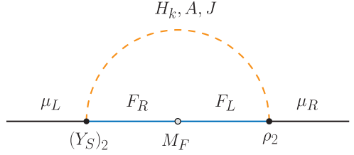
Figure 1: Dominant new physics contribution to the muon anomalous magnetic moment.

In our model, new contributions to the muon $g-2$ are induced at the 1-loop level, as shown in Fig. 1. This figure includes diagrams with the massive CP-even bosons $H_{k}$, with the massive CP-odd state $A$ and with the majoron $J$. For the massive states we use the analytical expressions given in [24], whereas the majoron contribution was recently computed in [7].

Higgs boson decays

The lightest CP-even scalar mass eigenstate, $H_{1}\equiv h$, can be identified with the $125$ GeV state discovered at the LHC. Therefore, it is crucial that its properties and decay channels match those observed, within the ranges allowed by the experimental errors. Since the observed state resembles the Higgs boson of the SM, this is guaranteed if the mixing angles in the CP-even scalar sector are sufficiently small. In this case, $h$ is made up mostly by the $S_{H}$ state, which has the properties of a SM Higgs. Thus, decays such as $h\rightarrow ZZ$, $WW$ are not modified substantially.

Higgs decays into a pair a of muons have been recently searched for by the ATLAS [27] and CMS [28] collaborations. Their data yields the following ratio in terms of the SM predicted value [6],

$$R_{h\mu\mu}=\frac{\text{BR}(h\to\mu\mu)^{\rm exp}}{\text{BR}(h\to\mu\mu)^{\rm SM}}=1.19\pm 0.39\,.$$ (94)

In our model, the mixing in the CP-even scalar sector may induce large deviations from the SM predicted ratio, $R_{h\mu\mu}=1$. Even if the mixing is tiny, the large $S$ and $\sigma$ couplings to muons, required if one wants to address the experimental anomaly in the muon anomalous magnetic moment, induce sizable contributions to $R_{h\mu\mu}$, which can largely deviate from $1$. An approximate analytical expression for $R_{h\mu\mu}$, valid under some simplifying assumptions, is provided in Appendix C.

Finally, $h$ can also decay invisibly to a pair of majorons. The current ATLAS limit on the invisible Higgs branching ratio translates into $\text{BR}(h\to JJ)<0.11$ at $95\%$ C.L. [29]. We take this constraints into account in our numerical analysis, using $\Gamma_{h}\approx\Gamma_{h}^{\rm SM}=4.1$ MeV for the total Higgs decay width [30].

5 Numerical results

In this Section we present our numerical results. These have been obtained by randomly scanning in the wide parameter space of the model and computing the observables discussed in the previous Section. All points in our scans are compatible with current neutrino oscillation data. This is achieved by using a Casas-Ibarra parametrization [31] for the $Y_{\nu}$ Yukawa matrix, which can be expressed as

$$Y_{\nu}=i\,\frac{\sqrt{2}}{v_{H}}\,D_{\sqrt{M_{R}}}\,O\,D_{\sqrt{m}}\,U^{\dagger}\,.$$ (95)

Here, we are working in the basis in which the $M_{R}$ matrix, defined in Eq. (40), is diagonal, with $M_{R}=\text{diag}\left(M_{1},M_{2},M_{3}\right)$. The neutrino mass matrix is diagonalized as $U^{T}\,m_{\nu}\,U=\text{diag}\left(m_{1},m_{2},m_{3}\right)$, where $U$ is a $3\times 3$ unitary matrix measured in neutrino oscillation experiments. We have also defined $D_{\sqrt{M_{R}}}=\text{diag}\left(\sqrt{M_{1}},\sqrt{M_{2}},\sqrt{M_{3}}\right)$ and introduced the $3\times 3$ orthogonal matrix $O$, such that $O^{T}O=OO^{T}=\mathbb{I}_{3}$. In our numerical analysis we assume normal neutrino mass ordering and randomly take neutrino oscillation parameters within the $3\,\sigma$ ranges obtained by the global fit [32].

Several parameters are chosen randomly in our scans. These are $v_{S}$, $v_{\sigma}$, the vector-like lepton mass $M_{F}$, the trilinear coupling $\mu$ as well as the $\rho$ and $Y_{S}$ Yukawa couplings, where the $\rho_{2}$ and the $\left(Y_{S}\right)_{2}$ upper bounds are chosen below the non-perturbative regime. In addition, the $\kappa$ Yukawa matrix has been taken diagonal, with $\kappa_{ii}$ also chosen randomly. All Yukawa couplings have been assumed to be real for simplicity. The ranges for the parameters that have been chosen randomly in our scans are shown on Tab. 2. We have chosen the VEV $v_{S}$ in the narrow range $[0.05,0.1]$ GeV. This choice is motivated by the fact that the doublet $S$ does not couple to quarks. A sizable $v_{S}$ VEV would imply a reduction of $v_{H}$ and, as a consequence of this, an increase in the Higgs boson couplings to quarks, already constrained by LHC data. Moreover, $v_{S}$ is also indirectly constrained due to its impact on the diagonal majoron couplings, see Eq. (88), and a small value is generally required. Furthermore, a small value for $v_{S}$ motivates a similarly small value for the $\mu$ trilinear coupling. Otherwise, the heavy CP-even scalars $H_{k}$ and the pseudoscalar $A$ become very heavy and their impact on the phenomenology negligible, see Eqs. (25) and (32). Finally, the scalar potential parameters $\lambda_{\sigma}=\lambda_{HS}^{(1)}=0.1$ and $\lambda_{S}=\lambda_{H\sigma}=\lambda_{HS}^{(2)}=\lambda_{S\sigma}=0.01$ have been fixed in all the scans. Note, however, that the exact choice for these quartic couplings is irrelevant for the observables we study. Also, the small values of $v_{S}$ and the quartics assure that SM precision observables are not substantially changed in our model.

Parameter	Range
$v_{S}$	$\left[0.05\,,\,0.1\right]$ GeV
$v_{\sigma}$	$\left[0.75\,,\,1.5\right]$ TeV
$M_{F}$	$\left[0.75\,,\,3\right]$ TeV
$\mu$	$\left[0.01\,,\,0.1\right]$ GeV
$\kappa_{ii}$	$\left[0.1\,,\,1\right]$
$\rho_{1}$	$\left[10^{-6}\,,\,1\right]\times 5\cdot 10^{-3}$
$\rho_{2}$	$\left[5\cdot 10^{-4}\,,\,\sqrt{4\pi}\right]$
$\rho_{3}$	$\left[0.05\,,\,1\right]\times 10^{-7}$
$\left(Y_{S}\right)_{1}$	$\left[0.01\,,\,1\right]\times 10^{-6}$
$\left(Y_{S}\right)_{2}$	$\left[0.1\,,\,\sqrt{4\pi}\right]$
$\left(Y_{S}\right)_{3}$	$\left[0.001\,,\,5\right]\times 10^{-7}$

Table 2: Ranges for the parameters that are randomly taken in our numerical analysis.

Our analysis has taken into account several experimental bounds. Starting with the LFV processes, we have checked that the branching ratios of the radiative processes $\ell_{\alpha}\rightarrow\ell_{\beta}\gamma$ as well as the 3-body decays $\ell^{-}_{\alpha}\rightarrow\ell^{-}_{\beta}\ell^{-}_{\beta}\ell^{+}_{\beta}$, $\ell^{-}_{\alpha}\rightarrow\ell^{-}_{\beta}\ell^{-}_{\gamma}\ell^{+}_{\gamma}$ and $\ell^{-}_{\alpha}\rightarrow\ell^{+}_{\beta}\ell^{-}_{\gamma}\ell^{-}_{\gamma}$ satisfy the existing bounds [6]. Regarding the decays $\ell_{\alpha}\rightarrow\ell_{\beta}\,J$, we have imposed the restrictions on the flavor violating couplings instead of the branching ratios. To do so, we have defined the combination

$$|S^{\beta\alpha}|=\left(\left|S_{L}^{\beta\alpha}\right|^{2}+\left|S_{R}^{\beta\alpha}\right|^{2}\right)^{1/2}\,$$ (96)

and imposed the bounds derived in [7], that is,

$$|S^{e\mu}|<5.3\times 10^{-11}\,,\quad|S^{e\tau}|<5.9\times 10^{-7}\,,\quad|S^{\mu\tau}|<7.6\times 10^{-7}\,.$$ (97)

On the flavor conserving side, it is well known that astrophysics imposes very stringent constraints on the majoron couplings to charged leptons. These are obtained by considering majoron-induced cooling processes in dense astrophysical media. Regarding the majoron coupling to electrons, Ref. [9] finds (at 90% C.L.)

$$\text{Im}\,S^{ee}<2.1\times 10^{-13}\,.$$ (98)

The majoron coupling to muons has also been studied, but only very recently [33, 9, 10]. Using the supernova SN1987A, Ref. [10] finds the limit 

$$\text{Im}\,S^{\mu\mu}<2.1\times 10^{-9}\,.$$ (99)

The impact of this bound on the phenomenology of the model will be studied in detail in the discussion that follows. We have also made sure here that the ratios

$$R_{Z\ell\ell}=\frac{\Gamma\left(Z\rightarrow\ell^{+}\ell^{-}\right)}{\Gamma_{SM}\left(Z\rightarrow\ell^{+}\ell^{-}\right)}\,,$$ (100)

where $\Gamma_{SM}\left(Z\rightarrow\ell^{+}\ell^{-}\right)$ is the SM predicted decay width, lie within the $95\%$ CL range, which is estimated to be $0.995<R_{Zee}<1.003$ and $0.993<R_{Z\mu\mu}<1.006$ [6]. With respect to Higgs decays, we have considered the very recent measurement of the process $h\to\mu\mu$, discussed in the previous Section, and we have rejected the points in our analysis outside the range compatible with Eq. (94) at $3\,\sigma$. Finally, points with $\text{BR}\left(h\to JJ\right)>0.11$ [29] have been discarded as well.

Our results for the LFV processes $\mu\to e\,\gamma$ and $\mu\to e\,J$ are shown in Fig. 2, which shows BR($\mu\to e\,\gamma$) as a function of BR($\mu\to e\,J$). The vertical line corresponds to the bound BR($\mu\to e\,J$) $<10^{-5}$, already discussed in the previous Section, while the horizontal line is the current limit BR($\mu\to e\,\gamma$) $<4.2\times 10^{-13}$, obtained by the MEG experiment [34]. Red points correspond to parameter points that respect all astrophysical bounds, namely the bounds on $S^{ee}$ and $S^{\mu\mu}$ in Eqs. (98) and (99), while the astrophysical bound on the majoron coupling to muons is violated in the blue points. Finally, the clear points are excluded due to one or several of the other experimental constraints mentioned above. First, as can be seen in this figure, our model is able to attain the current experimental bounds on BR($\mu\to e\,\gamma$) and BR($\mu\to e\,J$). Moreover, one finds no difference at all between blue and red points. This implies that the astrophysical bounds on the flavor-conserving couplings $S^{ee}$ and $S^{\mu\mu}$ have no impact on the results for the flavor-violating observables. We also observe that a correlation between BR($\mu\to e\,\gamma$) and BR($\mu\to e\,J$) exists, although these two observables depend on different combinations of parameters. However, it is easy to understand that they are not completely independent. In the limit $\rho_{1}=\left(Y_{S}\right)_{1}=0$, the vector-like fermion $F$ does not couple to electrons. In this case, the only contributions to $\mu-e$ LFV observables come from the $Y_{\nu}$ Yukawa matrix, which has entries of the size of $\sim 10^{-7}-10^{-6}$ and then leads to tiny LFV branching ratios. Therefore, sizable $\rho_{1}$ or $\left(Y_{S}\right)_{1}$ couplings are required in order to have observable LFV, and this applies both to $\mu\to e\,J$ and $\mu\to e\,\gamma$. Regarding other LFV processes, our numerical results also show that dipole contributions dominate the amplitude of the 3-body decay $\mu^{-}\to e^{-}e^{+}e^{-}$. This leads to strong correlations with $\mu\to e\,\gamma$, which always has a much larger branching ratio.

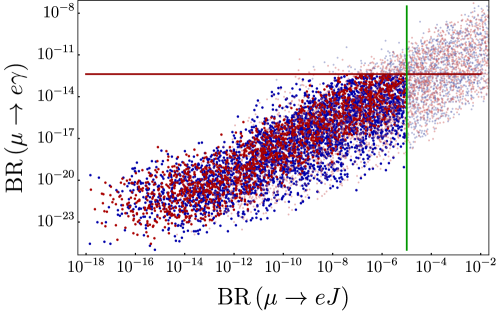
Figure 2: BR($\mu\to e\,J$) as a function of BR($\mu\to e\,J$).

Furthermore, in the region of parameter space covered by our numerical scan, it is easy to show that BR($\mu\to e\,J$) clearly correlates with the combination of parameters $v_{\sigma}\,\rho_{1}\,\rho_{2}\,M_{F}^{-2}$. From the expression of the majoron couplings to charged leptons in Eqs. (86) and (87) and the charged lepton mass matrix in Eq. (67), derived under the assumption $m_{\rho}\ll M_{F}$, and assuming $v_{S}\ll v_{H}$ and a large $\rho_{2}$ coupling, as motivated by the explanation of the muon $g-2$ anomaly, one can obtain the approximation for the off-diagonal $e-\mu$ coupling

$$|S^{e\mu}|\approx\frac{m_{\mu}\,v_{\sigma}}{M_{F}^{2}}\,\rho_{1}\,\rho_{2}\,.$$ (101)

We observe that, as long as the condition $m_{\rho}<M_{F}$ is satisfied, $|S^{e\mu}|$ actually grows when the $\rm U(1)_{L}$ symmetry breaking scale $v_{\sigma}$ increases. This result seems to go against the usual decoupling behavior expected when the new physics scale becomes larger. However, when $v_{\sigma}$ is increased, the mixing between the SM-like charged leptons and the vector-like lepton $F$ increases as well, hence enhancing the $\mu-e-J$ coupling. Eventually, when $v_{\sigma}$ is pushed above $M_{F}$, Eq. (101) becomes invalid and $\text{BR}(\mu\to e\,J)$ starts to decrease.

Several ideas to improve the current limit on $\mu\to e\,J$ have been put forward recently. As discussed in detail in [35, 36], the limit can be improved by the Mu3e experiment by looking for a bump in the continuous Michel spectrum. According to this analysis, $\mu\to e\,J$ branching ratios above $7.3\times 10^{-8}$ can be ruled out at 90% C.L.. Alternatively, reference [9] proposes a new phase of the MEG-II experiment with a Lyso calorimeter in the forward direction, increasing in this way the sensitivity for $\mu\to e\,J$. Therefore, $\mu\to e\,J$ already excludes a region of the parameter space of the model, and this region will be substantially enlarged in the future.

In what concerns $\tau$ decays, our choice of parameters suppresses all the LFV amplitudes. Since experimental limits in the $\tau$ sector are much weaker than for the muon, we do not show plots for LFV $\tau$ decays. We note, however, that one can saturate (some of) the experimental bounds also for $\tau$’s in our model, for the appropriate choice of (large) parameters in the 3rd generation. On the other hand, in our model it is not possible to have both, $\tau\to e\,\gamma$ and $\tau\to\mu\,\gamma$, with large rates at the same time, without running into conflict with $\mu\to e\,\gamma$.

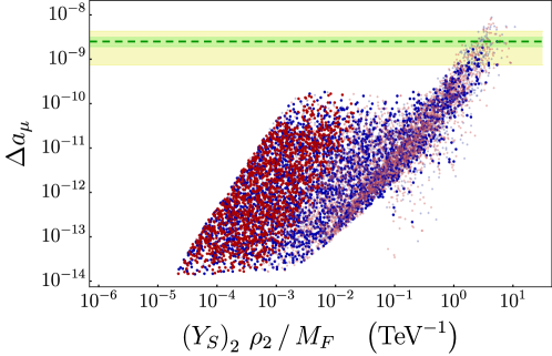
Figure 3: $\Delta a_{\mu}$ as a function of the combination $\left(Y_{S}\right)_{2}\rho_{2}/M_{F}$. Gray points are excluded due to one or several experimental bounds, but are shown for illustration.

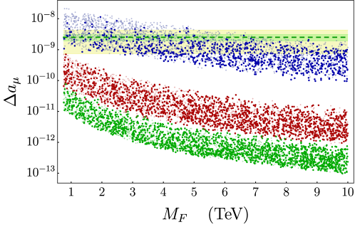
Figure 4: $\Delta a_{\mu}$ as a function of the vector-like mass $M_{F}$ for $\rho_{2}=\left(Y_{S}\right)_{2}=\sqrt{4\pi}$ (blue), $\rho_{2}=\left(Y_{S}\right)_{2}=1$ (red) and $\rho_{2}=\left(Y_{S}\right)_{2}=0.5$ (green).

Our model can also induce large contributions to the muon anomalous magnetic moment and address the current experimental anomaly. This is shown in Fig. 3. This figure displays $\Delta a_{\mu}$ as a function of the combination of parameters $\left(Y_{S}\right)_{2}\rho_{2}/M_{F}$, which enters the Feynman diagram in Fig. 1. The horizontal dashed line represents the experimental central value, while the green and yellow bands correspond to the $1\sigma$ and $3\sigma$ ranges, respectively.  As in the previous figure, the red points respect the astrophysical bounds on $S^{ee}$ and $S^{\mu\mu}$, while the blue points only respect the constraint on $S^{ee}$. Clear points are excluded due to one or several constraints, but are shown for illustration. We have found numerically that all diagrams, with massive scalars or with the majoron in the loop, may have comparable sizes. Interestingly, some points are found within the $1\sigma$ interval, hence providing a good explanation for the experimental value of the muon anomalous magnetic moment. These points require relatively light $F$ fermions (with masses of the order of $\sim 1-2$ TeV) and large (order $1$) $\rho_{2}$ and $\left(Y_{S}\right)_{2}$ Yukawa couplings. However, they violate the bound on $S^{\mu\mu}$ obtained from the supernova SN1987A, since this constraint necessarily implies a low value of $\rho_{2}$. In fact, we note that this figure displays a large concentration on points with low values of $\Delta a_{\mu}$ in a region where all the red points are found. This region is characterized by $\rho_{2}\ll 1$, and hence the dominant contributions to the muon $g-2$ do not come from the diagram in Fig. 1, but are mostly induced by diagrams proportional to $\left(Y_{S}\right)_{2}^{2}/M_{F}^{2}$. These diagrams have an external chirality flip that introduces an $m_{\mu}$ suppresing factor and then, as is generically found in a large class of models with this feature, $\Delta a_{\mu}$ can be at most $\sim 10^{-10}$.

Complementary information is provided by Fig. 4, which shows $\Delta a_{\mu}$ as a function of the vector-like mass $M_{F}$ for three different values of $\rho_{2}=\left(Y_{S}\right)_{2}$. Blue points corresponds to $\rho_{2}=\left(Y_{S}\right)_{2}=\sqrt{4\pi}$, red points to $\rho_{2}=\left(Y_{S}\right)_{2}=1$ and green points to $\rho_{2}=\left(Y_{S}\right)_{2}=0.5$. This figure has been obtained with a specific parameter scan in which $M_{F}\in\left[0.75\,,\,10\right]$ TeV, while the ranges for the other randomly chosen parameters are as in Tab. 2. As expected, all new physics contributions decrease for large $M_{F}$ and strongly depend on the value of the $\rho_{2}$ and $\left(Y_{S}\right)_{2}$ couplings. When $\rho_{2}=\left(Y_{S}\right)_{2}=0.5$, these are not large enough to address the muon $g-2$ anomaly, while when $\rho_{2}=\left(Y_{S}\right)_{2}=1$ this happens in a narrow region of the parameter space characterized by very light vector-like leptons, with masses $\lesssim 1$ TeV. Only when $\rho_{2}=\left(Y_{S}\right)_{2}=\sqrt{4\pi}$, one can find an explanation for the anomaly in a wide $M_{F}$ range. And even in this case, they eventually become too small to account for the measured muon $g-2$. However, this happens for very large vector-like masses. In fact, one finds that vector-like masses as large as $10$ TeV still allow for a $3\sigma$ explanation of the muon $g-2$ anomaly. Such a large mass would make the $F$ fermions unobservable at the LHC.

We turn our attention to Higgs boson decays. As already explained, the mixing in the CP-even scalar sector can induce large deviations from the SM predicted Higgs branching ratios. In particular, a large effective coupling to muons is induced in parameter points in which the muon $g-2$ anomaly is explained. This is shown in Fig. 5. Here we plot the ratio $R_{h\mu\mu}$, defined in Eq. (94), as a function of the lepton number breaking scale $v_{\sigma}$. The horizontal line represents the current central value, $R_{h\mu\mu}=1.19$ [6]. As in the previous plot, the vector-like mass $M_{F}$ is fixed to specific values in this figure: $M_{F}=1$ TeV (blue points), $M_{F}=3$ TeV (red points) and $M_{F}=5$ TeV (green points). In addition, $v_{S}=0.1$ GeV and $\rho_{2}=\left(Y_{S}\right)_{2}=\sqrt{4\pi}$ are fixed in this plot, while $\mu\in\left[0.05\,,\,50\right]$ GeV, $\rho_{1}\in\left[0.002\,,\,1.2\right]\times 10^{-6}$ and $\left(Y_{S}\right)_{1}\in\left[0.1\,,\,5\right]\times 10^{-7}$ are randomly varied and the rest of parameters are taken as in Tab. 2. Due to the large value chosen for $\rho_{2}$, the astrophysical bound on $S^{\mu\mu}$ is not respected in this plot. Imposing this constraint would imply $R_{h\mu\mu}\approx 1$. We observe that for large $v_{\sigma}$ and $M_{F}$ the new physics contributions become negligibly small and one finds $R_{h\mu\mu}=1$. However, for lower scales one finds many parameter points leading to large deviations from the SM predicted value. In particular, for $M_{F}=1$ TeV our scan reveals points with $R_{h\mu\mu}$ as large $\sim 1.4$ or as low as $\sim 0.3$. These extreme points are of course ruled out by the existing data, but serve as example of how easily Higgs decays into muons can deviate from the SM predictions in our setup.

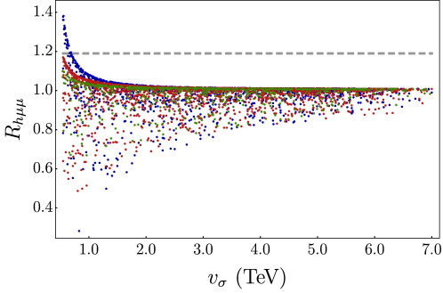
Figure 5: $R_{h\mu\mu}$ as a function of $v_{\sigma}$ for three fixed values of the vector-like mass $M_{F}$: $M_{F}=1$ TeV (blue), $M_{F}=3$ TeV (red) and $M_{F}=5$ TeV (green). The horizontal line represents the current central value, $R_{h\mu\mu}=1.19$ [6].

We finally note that the $R_{h\mu\mu}$ ratio does not correlate with other observables, due to the large number of independent contributions to the $h-\mu-\mu$ coupling, see Appendix C. For this reason, a definite prediction cannot be made. For instance, Eqs. (176)-(178) imply that for vanishing mixing in the scalar sector, $c_{\mu\mu}^{S_{\sigma}}=c_{\mu\mu}^{S_{S}}=0$ and $c_{\mu\mu}^{S_{H}}>c_{\mu\mu}^{\rm SM}$, hence predicting $R_{h\mu\mu}>1$. However, the $\alpha$ and $\beta$ angles never vanish and in fact one can find $R_{h\mu\mu}<1$ as well.

6 Summary

In this paper we have proposed a simple model that leads to sizable majoron flavor violating couplings to charged leptons. The particle spectrum is extended with the addition of two new scalar multiplets, as well as three right-handed neutrino singlets and a vector-like lepton. The SM symmetry is also extended with a continuous lepton number global symmetry. As a result of spontaneous symmetry breaking, neutrinos acquire non-zero Majorana masses via a type-I seesaw mechanism and a massless Goldstone boson appears in the spectrum, the majoron.

Thanks to large mixings between the SM charged leptons and the vector-like lepton, sizable majoron LFV couplings are generated at tree-level. Therefore, our model constitutes a simple example of a model with tree-level off-diagonal majoron couplings, not suppressed by neutrino masses. This induces plenty of signatures in experiments looking for LFV processes. In particular, we have shown that the decay $\mu\to e\,J$ can have large rates, close to the experimental limit. In fact, it already excludes part of the parameter space of the model.

As a by-product of our construction, other interesting phenomenological possibilities emerge: (i) an explanation to the current muon $g-2$ discrepancy can be provided in large parts of the parameter space of the model, easily finding points that address the anomaly even within $1\sigma$, and (ii) sizable deviations with respect to the SM predicted Higgs decay rates can be obtained, most notably in $h\to\mu\mu$. These two phenomenological possibilities provide additional handles on the model. We note, however, that an explanation of the muon $g-2$ anomaly would lead to tension with recent astrophysical bounds on the majoron coupling to muons.

In this work we have shown that as soon as the lepton sector is extended beyond the minimal models, exotic signatures appear, such as those including a massless majoron in the final state. This motivates the experimental search for processes like $\mu\to e\,J$ and estimulates the construction of new theoretical constructions that, in addition to neutrino masses, provide an understanding to other open questions.

Appendix A Proof of the pseudoscalar nature of the majoron couplings

Eq. (85) encodes the diagonal couplings of the majoron with the charged leptons of our model. Since the majoron is a pure pseudoscalar Goldstone boson, the coefficients $S^{\beta\beta}$ are purely imaginary. We are going to prove that this is indeed the case for the general scenario of $n$ singlet vector-like lepton pairs added to the SM leptons, with the same form of the couplings as the one defined in Eq. (7).  Let

$$M=\left(\begin{array}[]{cc}m_{1}&m_{2}\\ m_{3}&m_{4}\end{array}\right)\,$$ (102)

be a generic complex $(3+n)\times(3+n)$ complex matrix, given by the blocks $m_{1}$, $m_{2}$, $m_{3}$ and $m_{4}$, with dimensions $3\times 3$, $3\times n$, $n\times 3$ and $n\times n$, respectively. The singular value decomposition of the matrix $M$ is $V_{R}^{\dagger}\,M\,V_{L}=\widehat{M}$, where $V_{R}$ and $V_{L}$ are unitary matrices and $\widehat{M}=\text{diag}(M_{1},M_{2})$, with $M_{1}$ and $M_{2}$ $3\times 3$ and $n\times n$ real diagonal matrices, respectively, with positive entries. The interaction matrix of the majoron with the charged leptons can be written in the flavor basis as

$$N=\left(\begin{array}[]{cc}x\,m_{1}&(x+y)\,m_{2}\\ -y\,m_{3}&0\end{array}\right)\,,$$ (103)

where $N$ is another $(3+n)\times(3+n)$ matrix and $x,y\in\mathbb{R}$. Comparing with Eq. (82), the majoron coupling matrix in our model is given by $N\equiv A$ and corresponds to $m_{1}\equiv m_{e}$, $m_{2}\equiv m_{\rho}$, $m_{3}\equiv m_{S}$, $x\equiv v_{S}^{2}$ and $y\equiv v_{H}^{2}$.

First of all, we block-parametrize the unitary matrices $V_{R}$ and $V_{L}$ as

$$V_{R}^{\dagger}=\left(\begin{array}[]{cc}A&B\\ C&D\end{array}\right)\,,\quad V_{L}^{\dagger}=\left(\begin{array}[]{cc}E&F\\ G&H\end{array}\right)\,.$$ (104)

We also denote

$$e_{1}=\left(\begin{array}[]{c}\mathbb{I}_{3}\\ 0\end{array}\right)\,,\quad e_{2}=\left(\begin{array}[]{c}0\\ \mathbb{I}_{n}\end{array}\right)\,,$$ (105)

where $\mathbb{I}_{n}$ is the $n\times n$ identity matrix. Therefore, one obtains

$$\begin{split}\left(V_{R}^{\dagger}\,e_{1}\right)\left(V_{R}^{\dagger}\,e_{1}\right)^{\dagger}=\left(\begin{array}[]{cc}AA^{\dagger}&AC^{\dagger}\\ CA^{\dagger}&CC^{\dagger}\end{array}\right)\,,\\ \left(V_{R}^{\dagger}\,e_{2}\right)\left(V_{R}^{\dagger}\,e_{2}\right)^{\dagger}=\left(\begin{array}[]{cc}BB^{\dagger}&BD^{\dagger}\\ DB^{\dagger}&DD^{\dagger}\end{array}\right)\,.\end{split}$$ (106)

Analogously, one finds the following relations involving $V_{L}$:

$$\begin{split}\left(V_{L}^{\dagger}\,e_{1}\right)\left(V_{L}^{\dagger}\,e_{1}\right)^{\dagger}=\left(\begin{array}[]{cc}EE^{\dagger}&EG^{\dagger}\\ GE^{\dagger}&GG^{\dagger}\end{array}\right)\,,\\ \left(V_{L}^{\dagger}e_{2}\right)\left(V_{L}^{\dagger}e_{2}\right)^{\dagger}=\left(\begin{array}[]{cc}FF^{\dagger}&FH^{\dagger}\\ HF^{\dagger}&HH^{\dagger}\end{array}\right)\,.\end{split}$$ (107)

After these preliminaries, we note that the interaction matrix $N$ can be written as

$$N=x\,\left(\begin{array}[]{cc}m_{1}&m_{2}\\ 0&0\end{array}\right)+y\,\left(\begin{array}[]{cc}0&m_{2}\\ -m_{3}&0\end{array}\right)\,.$$ (108)

Therefore, if we prove that the combinations

$$V_{R}^{\dagger}\left(\begin{array}[]{cc}m_{1}&m_{2}\\ 0&0\end{array}\right)V_{L}\,,\quad V_{R}^{\dagger}\left(\begin{array}[]{cc}0&m_{2}\\ -m_{3}&0\end{array}\right)V_{L}$$ (109)

have real diagonal elements, then also $V_{R}^{\dagger}NV_{L}$ has real diagonal elements and the proof is complete. Let us consider the first term. It is easy to check that

$$\left(\begin{array}[]{cc}m_{1}&m_{2}\\ 0&0\end{array}\right)=e_{1}e_{1}^{T}M\,.$$ (110)

Then one can obtain

$$\begin{split}V_{R}^{\dagger}\left(\begin{array}[]{cc}m_{1}&m_{2}\\ 0&0\end{array}\right)V_{L}=V_{R}^{\dagger}e_{1}e_{1}^{T}MV_{L}=V_{R}^{\dagger}e_{1}e_{1}^{T}V_{R}\widehat{M}=\\ \left(V_{R}^{\dagger}\,e_{1}\right)\left(V_{R}^{\dagger}\,e_{1}\right)^{\dagger}\widehat{M}=\left(\begin{array}[]{cc}AA^{\dagger}M_{1}&AC^{\dagger}M_{2}\\ CA^{\dagger}M_{1}&CC^{\dagger}M_{2}\end{array}\right)\,.\end{split}$$ (111)

The diagonal terms of the resulting matrix are real because $AA^{\dagger}$ and $CC^{\dagger}$ are Hermitian matrices and $M_{1},M_{2}$ are real diagonal matrices. We now have to consider the second term in Eq. (108). It is possible to write

$$\left(\begin{array}[]{cc}0&m_{2}\\ -m_{3}&0\end{array}\right)=e_{1}\left(e_{1}^{T}Me_{2}\right)e_{2}^{T}-e_{2}\left(e_{2}^{T}Me_{1}\right)e_{1}^{T}\,.$$ (112)

Using similar manipulations as for the first term one finds

$$V_{R}^{\dagger}\left(\begin{array}[]{cc}0&m_{2}\\ -m_{3}&0\end{array}\right)V_{L}=\left(V_{R}^{\dagger}\,e_{1}\right)\left(V_{R}^{\dagger}\,e_{1}\right)^{\dagger}\widehat{M}\left(V_{L}^{\dagger}\,e_{2}\right)\left(V_{L}^{\dagger}\,e_{2}\right)^{\dagger}-\left(V_{R}^{\dagger}\,e_{2}\right)\left(V_{R}^{\dagger}\,e_{2}\right)^{\dagger}\widehat{M}\left(V_{L}^{\dagger}\,e_{1}\right)\left(V_{L}^{\dagger}\,e_{1}\right)^{\dagger}\,,$$ (113)

and, writing for the sake of brevity only the diagonal blocks of this expression, in the form of a column array, we obtain

$$\Big{[}V_{R}^{\dagger}\left(\begin{array}[]{cc}0&m_{2}\\ -m_{3}&0\end{array}\right)V_{L}\Big{]}_{\rm diag}=\left(\begin{array}[]{c}AA^{\dagger}M_{1}FF^{\dagger}+AC^{\dagger}M_{2}HF^{\dagger}\\ CC^{\dagger}M_{2}HH^{\dagger}+CA^{\dagger}M_{1}FH^{\dagger}\end{array}\right)-\left(\begin{array}[]{c}BB^{\dagger}M_{1}EE^{\dagger}+BD^{\dagger}M_{2}GE^{\dagger}\\ DD^{\dagger}M_{2}GG^{\dagger}+DB^{\dagger}M_{1}EG^{\dagger}\end{array}\right)\,.$$ (114)

The second terms in the sum cancel for both the upper and lower diagonal blocks, using the unitarity of $V_{L}$ and $V_{R}$. Then, using again unitarity in the following way

$$\begin{cases}AA^{\dagger}=1-BB^{\dagger}\\ EE^{\dagger}=1-FF^{\dagger}\\ CC^{\dagger}=1-DD^{\dagger}\\ GG^{\dagger}=1-HH^{\dagger}\,,\end{cases}$$ (115)

we finally end up with

$$\Big{[}V_{R}^{\dagger}\left(\begin{array}[]{cc}0&m_{2}\\ -m_{3}&0\end{array}\right)V_{L}\Big{]}_{\rm diag}=\left(\begin{array}[]{c}M_{1}FF^{\dagger}-BB^{\dagger}M_{1}\\ M_{2}HH^{\dagger}-DD^{\dagger}M_{2}\end{array}\right)\,,$$ (116)

and therefore the diagonal components of this matrix are purely real. This concludes the proof.

Appendix B Effective coefficients for flavor violating observables

In order to use the analytical results for the flavor violating observables provided in [21, 7], one must match the effective Lagrangian in these references to the specific model discussed here. We focus in particular on the 3-body lepton decays $\ell^{-}_{\alpha}\rightarrow\ell^{-}_{\beta}\ell^{-}_{\beta}\ell^{+}_{\beta}$, $\ell^{-}_{\alpha}\rightarrow\ell^{-}_{\beta}\ell^{-}_{\gamma}\ell^{+}_{\gamma}$ and $\ell^{-}_{\alpha}\rightarrow\ell^{+}_{\beta}\ell^{-}_{\gamma}\ell^{-}_{\gamma}$. These processes get tree-level contributions in our model from the three CP-even scalars $H_{k}$ ($k=1,2,3$), the $Z$-boson, the CP-odd scalar $A$ and the majoron $J$. The majoron contributions have been computed in [7]. Since all the other mediators are significantly heavier than the SM charged leptons, we can then parametrize their contributions by the effective Lagrangian

$$\mathcal{L}_{4\ell}=\sum_{\begin{subarray}{c}I=S,V,T\\ X,Y=L,R\end{subarray}}A^{I}_{XY}\bar{\ell^{\beta}}\Gamma_{I}P_{X}\ell^{\alpha}\bar{\ell^{\delta}}\Gamma_{I}P_{Y}\ell^{\gamma}+\text{h.c.}\,,$$ (117)

where we have defined $\Gamma_{S}=1$, $\Gamma_{V}=\gamma_{\mu}$ and $\Gamma_{T}=\sigma_{\mu\nu}$ and omitted flavor indices in the effective coefficients for the sake of simplicity. The coefficients $A^{I}_{XY}$ have dimensions of mass^-2. We will now give specific expressions for these coefficients in the model under consideration. In order to do that it proves convenient to define the following 3-component array

$$(c_{1},c_{2},c_{3})^{\beta\alpha}=(V^{R^{\dagger}}_{ee}Y_{e}V^{L}_{ee},V^{R^{\dagger}}_{ee}\rho V^{L}_{Fe},V^{R^{\dagger}}_{Fe}Y_{S}V^{L}_{ee})^{\beta\alpha}\,,$$ (118)

which encodes the interactions of the SM charged leptons with the CP-even scalars gauge eigenstates $\{S_{H},S_{\sigma},S_{S}\}$.

$\ell^{-}_{\alpha}\rightarrow\ell^{-}_{\beta}\ell^{-}_{\beta}\ell^{+}_{\beta}$

Recalling the definition of the $3\times 3$ unitary matrix $W$ given in Eq. (27), we get the following expressions for the effective coefficients $A^{I}_{XY}=(A^{I}_{XY})^{\beta\beta\beta\alpha}$.

$H_{k}$ contributions

$$A_{LL}^{S}=\frac{1}{2m_{H_{k}}^{2}}\sum_{i,j}\big{(}W_{ki}c_{i}^{\beta\beta}\big{)}\big{(}W_{kj}c_{j}^{\beta\alpha}\big{)}$$ (119)

$$A_{LR}^{S}=\frac{1}{2m_{H_{k}}^{2}}\sum_{i,j}\big{(}W_{ki}c_{i}^{\beta\beta}\big{)}\big{(}W_{kj}c_{j}^{\dagger^{\beta\alpha}}\big{)}$$ (120)

$$A_{RL}^{S}=\frac{1}{2m_{H_{k}}^{2}}\sum_{i,j}\big{(}W_{ki}c_{i}^{\dagger^{\beta\beta}}\big{)}\big{(}W_{kj}c_{j}^{\beta\alpha}\big{)}$$ (121)

$$A_{RR}^{S}=\frac{1}{2m_{H_{k}}^{2}}\sum_{i,j}\big{(}W_{ki}c_{i}^{\dagger{\beta\beta}}\big{)}\big{(}W_{kj}c_{j}^{\dagger{\beta\alpha}}\big{)}$$ (122)

$Z$ contributions

$$A_{LL}^{V}=-\frac{g^{2}}{4m_{W}^{2}}\Big{(}V^{L^{\dagger}}_{ee}V^{L}_{ee}-2\sin^{2}\theta_{W}\mathbb{I}\Big{)}^{\beta\beta}\Big{(}V^{L^{\dagger}}_{ee}V^{L}_{ee}\Big{)}^{\beta\alpha}$$ (123)

$$A_{LR}^{V}=0$$ (124)

$$A_{RL}^{V}=\frac{g^{2}}{2m_{W}^{2}}\sin^{2}\theta_{W}\Big{(}V^{L^{\dagger}}_{ee}V^{L}_{ee}\Big{)}^{\beta\alpha}$$ (125)

$$A_{RR}^{V}=0$$ (126)

Actually, the parametrization $V^{L(R)}=U^{L(R)}D^{L(R)}$ greatly simplifies the expressions. Taking into account the unitarity of $D^{L}_{e}$ one ends up with

$$A_{LL}^{V}=\frac{g^{2}}{4m_{W}^{2}M_{F}^{2}}\Big{[}1-2\sin^{2}\theta_{W}-\Big{(}D^{L^{\dagger}}_{e}\frac{m_{S}^{\dagger}m_{S}}{M_{F}^{2}}D^{L}_{e}\Big{)}^{\beta\beta}\Big{]}\Big{(}D^{L^{\dagger}}_{e}m_{S}^{\dagger}m_{S}D^{L}_{e}\Big{)}^{\beta\alpha}$$ (127)

$$A_{RL}^{V}=-\frac{g^{2}}{2m_{W}^{2}M_{F}^{2}}\sin^{2}\theta_{W}\Big{(}D^{L^{\dagger}}_{e}m_{S}^{\dagger}m_{S}D^{L}_{e}\Big{)}^{\beta\alpha}$$ (128)

$A$ contributions

From the profile of the massive CP-odd state $A$ given in Eq. (31) one can recover the interaction Lagrangian between $A$ and the charged leptons in the flavor basis

$$\mathcal{L}_{A\ell\ell}=-\frac{i\,A}{\sqrt{2}V^{2}}\left(\begin{array}[]{cc}\bar{e}_{R}&\bar{F}_{R}\end{array}\right)\left(\begin{array}[]{cc}-Y_{e}\,v_{S}v_{\sigma}&\rho\,v_{H}v_{S}\\ Y_{S}\,v_{H}v_{\sigma}&0\end{array}\right)\,\left(\begin{array}[]{c}e_{L}\\ F_{L}\end{array}\right)+\text{h.c.}\,.$$ (129)

Denoting the matrix in the previous equation as $B$ and transforming the Lagrangian to the mass basis, one can easily perform the matching with Eq. (117). We get the following expressions for the contributions of $A$ to the effective coefficients $A_{XY}^{I}=(A_{XY}^{I})^{\beta\beta\beta\alpha}$.

$$A_{LL}^{S}=-\frac{1}{2V^{4}m_{A}^{2}}\Big{(}V^{R^{\dagger}}BV^{L}\Big{)}^{\beta\beta}\Big{(}V^{R^{\dagger}}BV^{L}\Big{)}^{\beta\alpha}$$ (130)

$$A_{LR}^{S}=\frac{1}{2V^{4}m_{A}^{2}}\Big{(}V^{R^{\dagger}}BV^{L}\Big{)}^{\beta\beta}\Big{(}V^{L^{\dagger}}B^{\dagger}V^{R}\Big{)}^{\beta\alpha}$$ (131)

$$A_{RL}^{S}=\frac{1}{2V^{4}m_{A}^{2}}\Big{(}V^{L^{\dagger}}B^{\dagger}V^{R}\Big{)}^{\beta\beta}\Big{(}V^{R^{\dagger}}BV^{L}\Big{)}^{\beta\alpha}$$ (132)

$$A_{RR}^{S}=-\frac{1}{2V^{4}m_{A}^{2}}\Big{(}V^{L^{\dagger}}B^{\dagger}V^{R}\Big{)}^{\beta\beta}\Big{(}V^{L^{\dagger}}B^{\dagger}V^{R}\Big{)}^{\beta\alpha}$$ (133)

$\ell^{-}_{\alpha}\rightarrow\ell^{-}_{\beta}\ell^{-}_{\gamma}\ell^{+}_{\gamma}$

There are two types of Feynman diagrams contributing to this process. The first class involves a flavor conserving ($\gamma\gamma$) and a flavor violating ($\beta\alpha$) vertex, while in the second class both vertices violate flavor ($\beta\gamma$ and $\gamma\alpha$). Therefore, the matching with Eq. (117) would yield non vanishing contributions to both coefficients $(A_{XY}^{I})^{\gamma\gamma\beta\alpha}$ and $(A_{XY}^{I})^{\beta\gamma\gamma\alpha}$. One can actually Fierz transform the latter flavor structure into the former, thus in the following expressions we set $A_{XY}^{I}=(A_{XY}^{I})^{\gamma\gamma\beta\alpha}$. The Fierz transformations involved in the matching are the following, where the type of parenthesis indicates the fermion field which is contracted with the gamma matrix in brackets.

$$\begin{split}(P_{L})[P_{L}]=\frac{1}{2}(P_{L}][P_{L})+\frac{1}{8}(\sigma^{\mu\nu}P_{L}][\sigma_{\mu\nu}P_{L})\\ (P_{R})[P_{R}]=\frac{1}{2}(P_{R}][P_{R})+\frac{1}{8}(\sigma^{\mu\nu}P_{R}][\sigma_{\mu\nu}P_{R})\\ (P_{R})[P_{L}]=\frac{1}{2}(\gamma^{\mu}P_{L}][\gamma_{\mu}P_{R})\\ (\gamma^{\mu}P_{L})[\gamma_{\mu}P_{L}]=-(\gamma^{\mu}P_{L}][\gamma_{\mu}P_{L})\\ (\gamma^{\mu}P_{R})[\gamma_{\mu}P_{R}]=-(\gamma^{\mu}P_{R}][\gamma_{\mu}P_{R})\\ (\gamma^{\mu}P_{R})[\gamma_{\mu}P_{L}]=2(P_{L}][P_{R})\\ \end{split}$$ (134)

$H_{k}$ contributions

$$A_{LL}^{S}=\frac{1}{2m_{H_{k}}^{2}}\sum_{i,j}\Big{[}\big{(}W_{ki}c_{i}^{\gamma\gamma}\big{)}\big{(}W_{kj}c_{j}^{\beta\alpha}\big{)}-\frac{1}{2}\big{(}W_{ki}c_{i}^{\beta\gamma}\big{)}\big{(}W_{kj}c_{j}^{\gamma\alpha}\big{)}\Big{]}$$ (135)

$$A_{LL}^{T}=\frac{1}{2m_{H_{k}}^{2}}\sum_{i,j}\Big{[}-\frac{1}{8}\big{(}W_{ki}c_{i}^{\beta\gamma}\big{)}\big{(}W_{kj}c_{j}^{\gamma\alpha}\big{)}\Big{]}$$ (136)

$$A_{LR}^{S}=\frac{1}{2m_{H_{k}}^{2}}\sum_{i,j}\big{(}W_{ki}c_{i}^{\gamma\gamma}\big{)}\big{(}W_{kj}c_{j}^{\dagger^{\beta\alpha}}\big{)}$$ (137)

$$A_{RL}^{S}=\frac{1}{2m_{H_{k}}^{2}}\sum_{i,j}\big{(}W_{ki}c_{i}^{\dagger^{\gamma\gamma}}\big{)}\big{(}W_{kj}c_{j}^{\beta\alpha}\big{)}$$ (138)

$$A_{RR}^{S}=\frac{1}{2m_{H_{k}}^{2}}\sum_{i,j}\Big{[}\big{(}W_{ki}c_{i}^{\dagger{\gamma\gamma}}\big{)}\big{(}W_{kj}c_{j}^{\dagger{\beta\alpha}}\big{)}-\frac{1}{2}\big{(}W_{ki}c_{i}^{\dagger{\beta\gamma}}\big{)}\big{(}W_{kj}c_{j}^{\dagger{\gamma\alpha}}\big{)}\Big{]}$$ (139)

$$A_{RR}^{T}=\frac{1}{2m_{H_{k}}^{2}}\sum_{i,j}\Big{[}-\frac{1}{8}\big{(}W_{ki}c_{i}^{\dagger{\beta\gamma}}\big{)}\big{(}W_{kj}c_{j}^{\dagger{\gamma\alpha}}\big{)}\Big{]}$$ (140)

$$A_{LR}^{V}=\frac{1}{2m_{H_{k}}^{2}}\sum_{i,j}\Big{[}-\frac{1}{2}\big{(}W_{ki}c_{i}^{\beta\gamma}\big{)}\big{(}W_{kj}c_{j}^{\dagger{\gamma\alpha}}\big{)}\Big{]}$$ (141)

$$A_{RL}^{V}=\frac{1}{2m_{H_{k}}^{2}}\sum_{i,j}\Big{[}-\frac{1}{2}\big{(}W_{ki}c_{i}^{\dagger{\beta\gamma}}\big{)}\big{(}W_{kj}c_{j}^{\gamma\alpha}\big{)}\Big{]}$$ (142)

$Z$ contributions

$$A_{LL}^{V}=-\frac{g^{2}}{4m_{W}^{2}}\Big{[}\big{(}V^{L^{\dagger}}_{ee}V^{L}_{ee}-2\sin^{2}\theta_{W}\mathbb{I}\big{)}^{\gamma\gamma}\big{(}V^{L^{\dagger}}_{ee}V^{L}_{ee}\big{)}^{\beta\alpha}+\big{(}V^{L^{\dagger}}_{ee}V^{L}_{ee}\big{)}^{\beta\gamma}\big{(}V^{L^{\dagger}}_{ee}V^{L}_{ee}\big{)}^{\gamma\alpha}\Big{]}$$ (143)

$$A_{LR}^{V}=0$$ (144)

$$A_{RL}^{V}=\frac{g^{2}}{2m_{W}^{2}}\sin^{2}\theta_{W}\Big{(}V^{L^{\dagger}}_{ee}V^{L}_{ee}\Big{)}^{\beta\alpha}$$ (145)

$$A_{RR}^{V}=0$$ (146)

The parametrization $V^{L(R)}=U^{L(R)}D^{L(R)}$ also simplifies the expressions in this case. Thanks to the unitarity of $D_{e}^{L}$, we can write

$$\begin{split}A_{LL}^{V}=\frac{g^{2}}{4m_{W}^{2}M_{F}^{2}}\Big{[}\Big{(}1-2\sin^{2}\theta_{W}-\Big{(}D^{L^{\dagger}}_{e}\frac{m_{S}^{\dagger}m_{S}}{M_{F}^{2}}D^{L}_{e}\Big{)}^{\gamma\gamma}\Big{)}\Big{(}D^{L^{\dagger}}_{e}m_{S}^{\dagger}m_{S}D^{L}_{e}\Big{)}^{\beta\alpha}\\ -\frac{1}{M_{F}^{2}}\Big{(}D^{L^{\dagger}}_{e}m_{S}^{\dagger}m_{S}D^{L}_{e}\Big{)}^{\beta\gamma}\Big{(}D^{L^{\dagger}}_{e}m_{S}^{\dagger}m_{S}D^{L}_{e}\Big{)}^{\gamma\alpha}\Big{]}\end{split}$$ (147)

$$A_{RL}^{V}=-\frac{g^{2}}{2m_{W}^{2}M_{F}^{2}}\sin^{2}\theta_{W}\Big{(}D^{L^{\dagger}}_{e}m_{S}^{\dagger}m_{S}D^{L}_{e}\Big{)}^{\beta\alpha}$$ (148)

$A$ contributions

$$A_{LL}^{S}=-\frac{1}{2V^{4}m_{A}^{2}}\Big{[}\big{(}V^{R^{\dagger}}BV^{L}\Big{)}^{\gamma\gamma}\Big{(}V^{R^{\dagger}}BV^{L}\big{)}^{\beta\alpha}-\frac{1}{2}\big{(}V^{R^{\dagger}}BV^{L}\Big{)}^{\beta\gamma}\Big{(}V^{R^{\dagger}}BV^{L}\big{)}^{\gamma\alpha}\Big{]}$$ (149)

$$A_{LL}^{T}=-\frac{1}{2V^{4}m_{A}^{2}}\Big{[}-\frac{1}{8}\big{(}V^{R^{\dagger}}BV^{L}\Big{)}^{\beta\gamma}\Big{(}V^{R^{\dagger}}BV^{L}\big{)}^{\gamma\alpha}\Big{]}$$ (150)

$$A_{LR}^{S}=\frac{1}{2V^{4}m_{A}^{2}}\Big{(}V^{R^{\dagger}}BV^{L}\Big{)}^{\gamma\gamma}\Big{(}V^{L^{\dagger}}B^{\dagger}V^{R}\Big{)}^{\beta\alpha}$$ (151)

$$A_{RL}^{S}=\frac{1}{2V^{4}m_{A}^{2}}\Big{(}V^{L^{\dagger}}B^{\dagger}V^{R}\Big{)}^{\gamma\gamma}\Big{(}V^{R^{\dagger}}BV^{L}\Big{)}^{\beta\alpha}$$ (152)

$$A_{RR}^{S}=-\frac{1}{2V^{4}m_{A}^{2}}\Big{[}\big{(}V^{L^{\dagger}}B^{\dagger}V^{R}\Big{)}^{\gamma\gamma}\Big{(}V^{L^{\dagger}}B^{\dagger}V^{R}\big{)}^{\beta\alpha}-\frac{1}{2}\big{(}V^{L^{\dagger}}B^{\dagger}V^{R}\Big{)}^{\beta\gamma}\Big{(}V^{L^{\dagger}}B^{\dagger}V^{R}\big{)}^{\gamma\alpha}\Big{]}$$ (153)

$$A_{RR}^{T}=-\frac{1}{2V^{4}m_{A}^{2}}\Big{[}-\frac{1}{8}\big{(}V^{L^{\dagger}}B^{\dagger}V^{R}\Big{)}^{\beta\gamma}\Big{(}V^{L^{\dagger}}B^{\dagger}V^{R}\big{)}^{\gamma\alpha}\Big{]}$$ (154)

$$A_{RL}^{V}=\frac{1}{2V^{4}m_{A}^{2}}\Big{[}-\frac{1}{2}\big{(}V^{L^{\dagger}}B^{\dagger}V^{R}\Big{)}^{\beta\gamma}\Big{(}V^{R^{\dagger}}BV^{L}\big{)}^{\gamma\alpha}\Big{]}$$ (155)

$$A_{LR}^{V}=-\frac{1}{2V^{4}m_{A}^{2}}\Big{[}-\frac{1}{2}\big{(}V^{R^{\dagger}}BV^{L}\Big{)}^{\beta\gamma}\Big{(}V^{L^{\dagger}}B^{\dagger}V^{R}\big{)}^{\gamma\alpha}\Big{]}$$ (156)

$\ell^{-}_{\alpha}\rightarrow\ell^{+}_{\beta}\ell^{-}_{\gamma}\ell^{-}_{\gamma}$

In this process both vertices are necessarily flavor violating ($\gamma\beta$ and $\gamma\alpha$). This allows us to easily perform the matching with Eq. (117) and set in the following expressions $A_{XY}^{I}=(A_{XY}^{I})^{\gamma\beta\gamma\alpha}$.

$H_{k}$ contributions

$$A_{LL}^{S}=\frac{1}{2m_{H_{k}}^{2}}\sum_{i,j}\big{(}W_{ki}c_{i}^{\gamma\beta}\big{)}\big{(}W_{kj}c_{j}^{\gamma\alpha}\big{)}$$ (157)

$$A_{LR}^{S}=\frac{1}{2m_{H_{k}}^{2}}\sum_{i,j}\big{(}W_{ki}c_{i}^{\gamma\beta}\big{)}\big{(}W_{kj}c_{j}^{\dagger^{\gamma\alpha}}\big{)}$$ (158)

$$A_{RL}^{S}=\frac{1}{2m_{H_{k}}^{2}}\sum_{i,j}\big{(}W_{ki}c_{i}^{\dagger^{\gamma\beta}}\big{)}\big{(}W_{ki}c_{j}^{\gamma\alpha}\big{)}$$ (159)

$$A_{RR}^{S}=\frac{1}{2m_{H_{k}}^{2}}\sum_{i,j}\big{(}W_{ki}c_{i}^{\dagger{\gamma\beta}}\big{)}\big{(}W_{kj}c_{j}^{\dagger{\gamma\alpha}}\big{)}$$ (160)

$Z$ contributions

$$A_{LL}^{V}=-\frac{g^{2}}{4m_{W}^{2}}\Big{(}V^{L^{\dagger}}_{ee}V^{L}_{ee}\Big{)}^{\gamma\beta}\Big{(}V^{L^{\dagger}}_{ee}V^{L}_{ee}\Big{)}^{\gamma\alpha}$$ (161)

$$A_{LR}^{V}=0$$ (162)

$$A_{RL}^{V}=0$$ (163)

$$A_{RR}^{V}=0$$ (164)

Finally, using our previous definitions we can simplify Eq. (161) to

$$A_{LL}^{V}=-\frac{g^{2}}{4m_{W}^{2}M_{F}^{4}}\Big{(}D^{L^{\dagger}}_{e}m_{S}^{\dagger}m_{S}D^{L}_{e}\Big{)}^{\gamma\beta}\Big{(}D^{L^{\dagger}}_{e}m_{S}^{\dagger}m_{S}D^{L}_{e}\Big{)}^{\gamma\alpha}$$ (165)

$A$ contributions

$$A_{LL}^{S}=-\frac{1}{2V^{4}m_{A}^{2}}\Big{(}V^{R^{\dagger}}BV^{L}\Big{)}^{\gamma\beta}\Big{(}V^{R^{\dagger}}BV^{L}\Big{)}^{\gamma\alpha}$$ (166)

$$A_{LR}^{S}=\frac{1}{2V^{4}m_{A}^{2}}\Big{(}V^{R^{\dagger}}BV^{L}\Big{)}^{\gamma\beta}\Big{(}V^{L^{\dagger}}B^{\dagger}V^{R}\Big{)}^{\gamma\alpha}$$ (167)

$$A_{RL}^{S}=\frac{1}{2V^{4}m_{A}^{2}}\Big{(}V^{L^{\dagger}}B^{\dagger}V^{R}\Big{)}^{\gamma\beta}\Big{(}V^{R^{\dagger}}BV^{L}\Big{)}^{\gamma\alpha}$$ (168)

$$A_{RR}^{S}=-\frac{1}{2V^{4}m_{A}^{2}}\Big{(}V^{L^{\dagger}}B^{\dagger}V^{R}\Big{)}^{\gamma\beta}\Big{(}V^{L^{\dagger}}B^{\dagger}V^{R}\Big{)}^{\gamma\alpha}$$ (169)

Appendix C $R_{h\mu\mu}$ analytical expression

In our model, the $R_{h\mu\mu}$ ratio can be approximately written as

$$R_{h\mu\mu}=\frac{\text{BR}(h\to\mu\mu)}{\text{BR}(h\to\mu\mu)^{\rm SM}}\approx\left(\frac{c_{\mu\mu}^{S_{H}}+c_{\mu\mu}^{S_{\sigma}}+c_{\mu\mu}^{S_{S}}}{c_{\mu\mu}^{\rm SM}}\right)^{2}\,,$$ (170)

where

$$c_{\mu\mu}^{\rm SM}=\frac{gm_{\mu}}{2m_{W}}$$ (171)

is the SM Higgs coupling to a pair of muons and $c_{\mu\mu}^{S_{H}}$, $c_{\mu\mu}^{S_{\sigma}}$ and $c_{\mu\mu}^{S_{S}}$ denote the contributions from the gauge eigenstates $S_{H}$, $S_{\sigma}$ and $S_{S}$, respectively. These couplings are given by

$$c_{\mu\mu}^{S_{H}} \approx\frac{1}{\sqrt{2}}Y_{e_{22}}V^{R^{\dagger}}_{22}V^{L^{\dagger}}_{22}\,$$ (172)

$$c_{\mu\mu}^{S_{\sigma}} \approx\frac{1}{\sqrt{2}}\sin\alpha\rho_{2}V^{R^{\dagger}}_{22}V^{L^{\dagger}}_{24}\,,$$ (173)

$$c_{\mu\mu}^{S_{S}} \approx\frac{1}{\sqrt{2}}\sin\beta Y_{S_{2}}V^{R^{\dagger}}_{24}V^{L^{\dagger}}_{22}\,,$$ (174)

where we have assumed $\rho_{1},\rho_{3}\ll\rho_{2}$ and $Y_{S_{1}},Y_{S_{3}}\ll Y_{S_{2}}$, as motivated by the explanation of the muon $g-2$ anomaly and the stringent constraints from lepton flavor violating observables. Furthermore, we have introduced the mixing angles $\alpha$, $\beta$ and $\gamma$. The CP-even scalar mass matrix $\mathcal{M}_{R}^{2}$ in Eq.(25) is diagonalized by the unitary matrix $R$ which, assuming small mixing angles, can be parametrized as

$$R=\left(\begin{array}[]{ccc}1&\sin\alpha&\sin\beta\\ -\sin\alpha&1&\sin\gamma\\ -\sin\beta&-\sin\gamma&1\end{array}\right)\,,$$ (175)

where $\alpha,\beta,\gamma\ll 1$. Using now Eqs. (63)-(67) we finally obtain

$$c_{\mu\mu}^{S_{H}} \approx\frac{m_{\mu}}{v_{H}}+\frac{Y_{S_{2}}v_{S}\rho_{2}v_{\sigma}}{2M_{F}v_{H}}\left[1-\left(\frac{\rho_{2}v_{\sigma}}{2M_{F}}\right)^{2}\right]\,,$$ (176)

$$c_{\mu\mu}^{S_{\sigma}} \approx\frac{\rho_{2}Y_{S_{2}}v_{S}}{2M_{F}}\,\sin\alpha\,,$$ (177)

$$c_{\mu\mu}^{S_{S}} \approx-\frac{\rho_{2}Y_{S_{2}}v_{\sigma}}{2M_{F}}\left[1-\left(\frac{\rho_{2}v_{\sigma}}{2M_{F}}\right)^{2}\right]\sin\beta\,.$$ (178)

References

- [1] Y. Chikashige, R. N. Mohapatra, and R. D. Peccei, “Spontaneously Broken Lepton Number and Cosmological Constraints on the Neutrino Mass Spectrum,” Phys. Rev. Lett. 45 (1980) 1926.
- [2] Y. Chikashige, R. N. Mohapatra, and R. D. Peccei, “Are There Real Goldstone Bosons Associated with Broken Lepton Number?,” Phys. Lett. B 98 (1981) 265–268.
- [3] J. Schechter and J. W. F. Valle, “Neutrino Decay and Spontaneous Violation of Lepton Number,” Phys. Rev. D 25 (1982) 774.
- [4] G. B. Gelmini and M. Roncadelli, “Left-Handed Neutrino Mass Scale and Spontaneously Broken Lepton Number,” Phys. Lett. B 99 (1981) 411–415.
- [5] C. Aulakh and R. N. Mohapatra, “Neutrino as the Supersymmetric Partner of the Majoron,” Phys. Lett. B 119 (1982) 136–140.
- [6] Particle Data Group Collaboration, P. A. Zyla et al., “Review of Particle Physics,” PTEP 2020 no. 8, (2020) 083C01.
- [7] P. Escribano and A. Vicente, “Ultralight scalars in leptonic observables,” JHEP 03 (2021) 240, arXiv:2008.01099 [hep-ph].
- [8] EXO-200 Collaboration, J. B. Albert et al., “Search for Majoron-emitting modes of double-beta decay of 136Xe with EXO-200,” Phys. Rev. D 90 no. 9, (2014) 092004, arXiv:1409.6829 [hep-ex].
- [9] L. Calibbi, D. Redigolo, R. Ziegler, and J. Zupan, “Looking forward to Lepton-flavor-violating ALPs,” arXiv:2006.04795 [hep-ph].
- [10] D. Croon, G. Elor, R. K. Leane, and S. D. McDermott, “Supernova Muons: New Constraints on ’ Bosons, Axions and ALPs,” JHEP 01 (2021) 107, arXiv:2006.13942 [hep-ph].
- [11] R. Ballou et al., “Latest Results of the OSQAR Photon Regeneration Experiment for Axion-Like Particle Search,” in 10th Patras Workshop on Axions, WIMPs and WISPs. 10, 2014. arXiv:1410.2566 [hep-ex].
- [12] A. Pilaftsis, “Astrophysical and terrestrial constraints on singlet Majoron models,” Phys. Rev. D 49 (1994) 2398–2404, arXiv:hep-ph/9308258.
- [13] J. Heeck and H. H. Patel, “Majoron at two loops,” Phys. Rev. D 100 no. 9, (2019) 095015, arXiv:1909.02029 [hep-ph].
- [14] Y. Cheng, C.-W. Chiang, X.-G. He, and J. Sun, “Flavor-changing Majoron interactions with leptons,” Phys. Rev. D 104 no. 1, (2021) 013001, arXiv:2012.15287 [hep-ph].
- [15] J. Sun, Y. Cheng, and X.-G. He, “Structure Of Flavor Changing Goldstone Boson Interactions,” JHEP 04 (2021) 141, arXiv:2101.06055 [hep-ph].
- [16] T. Aoyama et al., “The anomalous magnetic moment of the muon in the Standard Model,” Phys. Rept. 887 (2020) 1–166, arXiv:2006.04822 [hep-ph].
- [17] Muon g-2 Collaboration, B. Abi et al., “Measurement of the Positive Muon Anomalous Magnetic Moment to 0.46 ppm,” Phys. Rev. Lett. 126 no. 14, (2021) 141801, arXiv:2104.03281 [hep-ex].
- [18] M. Hirsch, A. Vicente, J. Meyer, and W. Porod, “Majoron emission in muon and tau decays revisited,” Phys. Rev. D 79 (2009) 055023, arXiv:0902.0525 [hep-ph]. [Erratum: Phys.Rev.D 79, 079901 (2009)].
- [19] W. Grimus and L. Lavoura, “The Seesaw mechanism at arbitrary order: Disentangling the small scale from the large scale,” JHEP 11 (2000) 042, arXiv:hep-ph/0008179.
- [20] L. Lavoura, “General formulae for ,” Eur. Phys. J. C 29 (2003) 191–195, arXiv:hep-ph/0302221.
- [21] A. Abada, M. E. Krauss, W. Porod, F. Staub, A. Vicente, and C. Weiland, “Lepton flavor violation in low-scale seesaw models: SUSY and non-SUSY contributions,” JHEP 11 (2014) 048, arXiv:1408.0138 [hep-ph].
- [22] A. Jodidio et al., “Search for Right-Handed Currents in Muon Decay,” Phys. Rev. D 34 (1986) 1967. [Erratum: Phys.Rev.D 37, 237 (1988)].
- [23] TWIST Collaboration, R. Bayes et al., “Search for two body muon decay signals,” Phys. Rev. D 91 no. 5, (2015) 052020, arXiv:1409.0638 [hep-ex].
- [24] A. Crivellin, M. Hoferichter, and P. Schmidt-Wellenburg, “Combined explanations of and implications for a large muon EDM,” Phys. Rev. D 98 no. 11, (2018) 113002, arXiv:1807.11484 [hep-ph].
- [25] Muon g-2 Collaboration, G. W. Bennett et al., “Final Report of the Muon E821 Anomalous Magnetic Moment Measurement at BNL,” Phys. Rev. D 73 (2006) 072003, arXiv:hep-ex/0602035.
- [26] S. Borsanyi et al., “Leading hadronic contribution to the muon magnetic moment from lattice QCD,” Nature 593 no. 7857, (2021) 51–55, arXiv:2002.12347 [hep-lat].
- [27] ATLAS Collaboration, G. Aad et al., “A search for the dimuon decay of the Standard Model Higgs boson with the ATLAS detector,” Phys. Lett. B 812 (2021) 135980, arXiv:2007.07830 [hep-ex].
- [28] CMS Collaboration, A. M. Sirunyan et al., “Evidence for Higgs boson decay to a pair of muons,” JHEP 01 (2021) 148, arXiv:2009.04363 [hep-ex].
- [29] ATLAS Collaboration, “Combination of searches for invisible Higgs boson decays with the ATLAS experiment,”.
- [30] LHC Higgs Cross Section Working Group Collaboration, D. de Florian et al., “Handbook of LHC Higgs Cross Sections: 4. Deciphering the Nature of the Higgs Sector,” arXiv:1610.07922 [hep-ph].
- [31] J. A. Casas and A. Ibarra, “Oscillating neutrinos and ,” Nucl. Phys. B 618 (2001) 171–204, arXiv:hep-ph/0103065.
- [32] P. F. de Salas, D. V. Forero, S. Gariazzo, P. Martínez-Miravé, O. Mena, C. A. Ternes, M. Tórtola, and J. W. F. Valle, “2020 global reassessment of the neutrino oscillation picture,” JHEP 02 (2021) 071, arXiv:2006.11237 [hep-ph].
- [33] R. Bollig, W. DeRocco, P. W. Graham, and H.-T. Janka, “Muons in Supernovae: Implications for the Axion-Muon Coupling,” Phys. Rev. Lett. 125 no. 5, (2020) 051104, arXiv:2005.07141 [hep-ph]. [Erratum: Phys.Rev.Lett. 126, 189901 (2021)].
- [34] MEG Collaboration, A. M. Baldini et al., “Search for the lepton flavour violating decay with the full dataset of the MEG experiment,” Eur. Phys. J. C 76 no. 8, (2016) 434, arXiv:1605.05081 [hep-ex].
- [35] Mu3e Collaboration, A.-K. Perrevoort, “The Rare and Forbidden: Testing Physics Beyond the Standard Model with Mu3e,” SciPost Phys. Proc. 1 (2019) 052, arXiv:1812.00741 [hep-ex].
- [36] A.-K. Perrevoort, Sensitivity Studies on New Physics in the Mu3e Experiment and Development of Firmware for the Front-End of the Mu3e Pixel Detector. PhD thesis, Ruprecht-Karls-Universität Heidelberg, 2018.